A Dual-Attention Aware Deep Convolutional Neural Network for Early Alzheimer’s Detection

Abstract

Alzheimer’s disease (AD) represents the primary form of neurodegeneration, impacting millions of individuals each year and causing progressive cognitive decline. Accurately diagnosing and classifying AD using neuroimaging data presents ongoing challenges in medicine, necessitating advanced interventions that will enhance treatment measures. In this research, we introduce a dual - attention - enhanced deep learning (DL) framework for classifying AD from neuroimaging data. Combined spatial and self-attention mechanisms play a vital role in emphasizing focus on neurofibrillary tangles and amyloid plaques from the MRI images, which are difficult to discern with regular imaging techniques. Results demonstrate that our model yielded remarkable performance in comparison to existing state-of-the-art (SOTA) convolutional neural networks (CNNs), with an accuracy of 99.1%. Moreover, it recorded remarkable metrics, with an F1-Score of 99.31%, a precision of 99.24%, and a recall of 99.51% . These results highlight the promise of cutting-edge DL methods in medical diagnostics, contributing to highly reliable and more efficient healthcare solutions.

Keywords Alzhiemer’s Disease  $\cdot$ Medical Imaging  $\cdot$ DL  $\cdot$ Attention Mechanisms

1 Introduction

Characterized by chronic neurodegeneration, Alzheimer’s disease results in systematic brain neuron deterioration. It impacts cognitive abilities and reduces the capacity to execute basic tasks, and is the major cause of dementia in elderly people [1]. AD causes an individual to suffer from memory loss, difficulty in speaking or understanding, disorientation, mood swings, and unpredictable behavior. AD also causes the presence of abnormal masses (amyloid plaques) and tangled strands of fibers known as the brain’s neurofibrillary tangles along with loss of connection between neurons. These are considered the key features of AD [2]. The disease primarily impacts regions of the brain that are responsible for cognition, memory, and communication. The hippocampus and the entorhinal cortex of the brain, essential for forming memories, are the first to be affected. As more neurons die, additional parts of the brain are affected causing the brain to shrink. The progression of AD varies among individuals causing the symptoms to be even more severe.

The underlying cause of AD is still unclear, but it is believed to be a amalgamation of genetic factors along with lifestyle and environmental conditions. Age is considered to be the most significant risk factor, with most cases diagnosed in those over 65 years old. A family history of AD can also increase the risk. However, genetics alone does not cover the entirety of the causes behind the disease. AD is diagnosed through a comprehensive evaluation of medical history, physical examination, and cognitive and neuropsychological tests. MRI Scans play a crucial role in detecting AD by providing detailed images of the brain, including the shape and the size of the brain regions. Using these images, doctors can identify the changes in the brain over time, which may support a diagnosis of AD. Comparing them with the patient’s history, a memory decline and other cognitive functions is considered a primary symptom of dementia [3].

In our work, we aim to contribute to the advancement of AD detection, offering an effective method to enhance the quality of medical diagnostics with the help machine learning (ML), artificial intelligence (AI), and DL. Sophisticated algorithms include CNNs (CNNs) and advanced DL techniques for accurate identification of AD. DL has significantly influenced the field of AD detection by employing sophisticated methods that can analyze a wide range of data. The key contribution of DL in AD detection is its ability to process complex data, and images obtained from MRI scans, to identify patterns of degeneration in the brain. CNNs outperforms at extracting features and intricate patterns from images. These models can learn patterns from the data and help us identify whether the patient has AD or not. By identifying AD early with these advanced algorithms, we can potentially slow down its progress and lead to better outcomes. [4]

The use of DL algorithms can help automate the process of analyzing the MRI scans of patients, hence reducing the need for doctors to manually analyze those MRI scans. This automation speeds up the process of diagnosis, allowing healthcare professionals to focus more on patient care. DL approaches show an improvement in terms of performance and show promising results for the identification of AD [5].

In this research, we introduce a dual-attention-enabled deep CNN capable of extracting key high-level and low-level features effectively, aiding healthcare professionals in accurately identifying the abnormalities in the brain in a fast and efficient way. For this purpose, we utilized the OASIS-1 (Open Access Series of Imaging Studies) dataset [6], containing cross-sectional MRI data in non-demented, young, demented older adults, and middle-aged. We compared our work with existing research and various other high-performing CNN models. Our findings indicate that our model surpasses results from previous worka and SOTA CNNs, demonstrating its capabilities in highly accurate feature extraction and classification.

2 Related Works

Helaly et al. [7] underscored the efficacy of DL techniques, particularly CNNs (CNNs), in the early detection of AD through Biomedical image analysis. This study prioritizes using multi-class classification to classify different stages of AD, along with binary classification to differentiate between specific stage pairs, facilitating precise diagnosis and treatment planning. Transfer learning, exemplified by fine-tuning pre-trained models like VGG19, optimizes the utilization of available data for improved detection accuracy. Proposals for remote AD screening applications address the challenges posed by the COVID-19 pandemic, providing patients with a convenient and safe means of assessment. Evaluation metrics such as specificity, accuracy, and sensitivity serve as benchmarks for assessing model performance while emphasizing computational efficiency and practicality in clinical settings. Overall, these findings suggest promising avenues for further research, including the exploration of novel architectures and the integration of advanced technologies to enhance the accuracy and usability of remote screening tools. Venugopalan et al. [8] delved into the realm of AD detection, recognizing the limitations of single-data modality approaches and advocating for integrating multiple data sources for a comprehensive analysis of AD staging. The authors propose a new approach to fully analyze magnetic resonance imaging (MRI), single nucleotide polymorphisms (SNPs) and clinical test data using DL techniques specifically stacked denoising auto-encoders for clinical and genetic data, 3D-CNNs for imaging data. Patients were classified into three categories: AD, mild cognitive impairment (MCI), and controls (CN). The method goes beyond classification as they introduce a novel means of clustering and perturbation analysis to detect the best features learned by deep models. They showed the superiority of deep models over other models such as random forests, support vector machines, k-nearest neighbors, decision trees in using AD Neuroimaging Initiative (ADNI) data. Furthermore, they show that multi-modality data integration improves performance across several metrics compared to single-modality models. It is worth noting that these models also identify key differences in the hippocampus, amygdala areas of the brain, and Rey Auditory Verbal Learning Test (RAVLT), which is consistent with previous AD literature. The study highlights the potential of DL for clinical decision making in diseases like AD as well as importance of early diagnosis considering that it is associated with high disease burden and poor diagnostic accuracy rates in current medical practices.

Ahila et al. [9] presented a study wherein they addressed the formidable challenge posed by AD in modern healthcare. AD is both progressive and incurable, necessitating early detection for effective management, a task often hindered by the lack of precision in current diagnostic approaches. Leveraging neuroimaging techniques, particularly Positron Emission Tomography (PET), the authors aim to bridge this gap through the development of a CAD (Computer-Aided Diagnosis) system. Previous methodologies primarily relied on image processing techniques for feature extraction, yielding variable success rates. In response, Ahila et al. propose an advanced CAD system built upon CNNs (CNNs) to enhance diagnostic accuracy. Their approach is rigorously evaluated on a dataset comprising 855 patients from the AD Neuroimaging Initiative (ADNI) database, yielding remarkable performance metrics with an sensitivity of 96%, specificity of 94%, and accuracy of 96%. These findings underscore the significant potential of DL neural networks in revolutionizing AD diagnosis, surpassing conventional methods detailed in the existing literature. Puente-Castro et al. [10] addressed the need for early identification of AD by developing a system that identifies the presence of AD in MRIs, an underutilized modality for AD diagnosis. To improve performance, they use Transfer Learning (TL) with data obtained from AD Neuroimaging Initiative (ADNI) and OASIS datasets.. Their findings reveal that AD-related damages and stages can be distinguished in sagittal MRIs, with results comparable to those obtained using horizontal-plane MRIs. Despite the less common use of sagittal-plane MRIs, this study demonstrates their effectiveness in identifying AD in early stages, suggesting avenues for future research. Additionally, the authors highlight the cost-saving potential of DL models in fields where data acquisition is expensive, emphasizing TL as a valuable tool for achieving robust performance with limited examples.

Zhang et al. [11] addressed the pressing need for early detetction of AD and mild cognitive impairment (MCI) by proposing a novel DL approach. Their approach systematically evaluates CNN models of different capacities and structures to determine the most suitable model for AD diagnosis. Additionally, they introduced a Two-stage Random RandAugment (TRRA) data augmentation strategy to mitigate overfitting and improve classification performance. The study incorporates a method utilizing Grad-CAM++ to produce heatmaps, thereby improving model transparency. Evaluation is performed across publicly available data for distinguishing cognitively normal (CN) vs AD and stable MCI (sMCI) vs. progressive MCI (pMCI) which shows superior performance compared to existing methods. This research contributes to advancing computer-aided diagnostic methods for AD and MCI, addressing challenges like overfitting, data leakage, and opaque diagnoses. Liu et al. [12] presented a novel ML method for identifying AD, contributing to the growing body of research aimed at improving diagnostic accuracy in AD. While the article undergoes final revisions before publication, the authors provide early visibility into their work. Their approach is situated within the broader context of ML applications in AD diagnosis, addressing the pressing need for reliable and efficient diagnostic tools. By leveraging advanced ML techniques, Liu et al. aim to enhance the efficiency and accuracy of AD identification, thereby facilitating early detection for improved patient outcomes. The study represents a significant contribution to the field, offering potential advancements in AD diagnosis that could have profound implications for clinical practice and patient care.

Chang et al. [13] provided a comprehensive literature survey on ML techniques and biomarkers for the diagnosis of AD, addressing the limitations of current diagnostic methods that rely on costly and invasive procedures. Their meta-analysis highlights the growing interest in leveraging AI, particularly ML tools, for precision diagnosis of AD. Beyond traditional biomarkers such as amyloid-$\beta$1-42 (A$\beta$42) and tau proteins, the authors explore emerging biomarkers associated with various mechanisms of AD pathology, including neuronal injury, synaptic dysfunction, and neuroinflammation. Notably, they discuss the potential of ML algorithms such as naïve Bayes, random forest, logistic regression, and support vector machine to integrate multiple variables and improve diagnostic accuracy. By emphasizing the importance of rapid and cost-effective diagnostic tools, Chang et al. underscore the potential of ML coupled with novel biomarkers to enhance sensitivity and specificity in diagnosing AD, offering promising avenues for future research and clinical practice. Ebrahimighahnavieh et al. [14] conducted a literature review on the application of DL techniques in detecting AD from neuroimaging data. This review addresses the need for reliable and efficient diagnostic tools for AD, a complex neurodegenerative disorder with significant clinical implications. By synthesizing existing research, the authors provide insights into the DL methodologies for AD detection, highlighting key findings, methodologies, and challenges. Their review sheds light on the potentiality of DL approaches to elevate the accuracy of AD diagnosis, offering valuable perspectives for future research directions and clinical applications in the field of neuroimaging-based AD detection.

Ji et al. [15] contributed to the field of AD diagnosis by focusing on early detection using ConvNets applied to MRI data. Their research addresses the critical need for early confirmation of AD to facilitate timely intervention and treatment initiation. While previous ML methods relied on manually crafted features and complex architectures, the authors leverage DL algorithms for pattern classification. Their approach involves utilizing ensemble learning methods to improve performance. Three base ConvNets are compared, demonstrating accuracy rates of up to 97.65% for mild cognitive normal/impairment control classifications and 88.37% for AD/mild cognitive impairment. By evaluating their method on a dataset from the ADNI, Ji et al . showcase the potential of DL techniques for AD diagnosis, offering promising avenues for further research and clinical application in health informatics. Khan et al. [16] proposed an advanced multi-modal ML approach for AD prognosis. They introduced a five-stage ML pipeline integrating data transformation, feature selection, and a random forest classifier. This methodology aimed to classify longitudinal MRI data into demented and non-demented categories, achieving high accuracy. Their study demonstrated the effectiveness of this approach in automating AD diagnosis and monitoring, highlighting its potential for clinical application and further improvements in diagnostic accuracy.

Orouskhani et al. [17] came up with a novel conditional deep triplet network for AD detection from structural MRI. They addressed the challenge of limited dataset samples in DL by employing deep metric learning techniques. To enhance model performance, the network utilizes a conditional loss function inspired by the VGG16 architecture. Their experiments on the OASIS dataset demonstrated superior performance over existing models, highlighting the effectiveness of their approach in improving Alzheimer’s diagnosis accuracy through robust feature learning. Saleh et al. [18] proposed an AD classification model using DenseNet with embedded healthcare decision support. They leveraged transfer learning to enhance the classification of AD into three classes based on MRI data. The study demonstrated that DenseNet architecture, with appropriate data augmentation techniques, significantly improves classification accuracy and generalization capabilities. Their approach not only outperformed other models but also integrated a support system, providing insights for clinical decision-making in AD diagnosis. Dua et al. [19] proposed a novel LSTM-CNN-RNN amalgamation approach for detecting AD using MRI scans. They aimed to accurately assess dementia levels early to facilitate timely medical intervention. Addressing the limitations of existing models like SVM and CNN for large datasets, their approach combines CNN for feature extraction with RNN and LSTM for sequence learning. Utilizing ensemble techniques such as Bagging, they achieved significant improvements in accuracy, reaching 92.22%. This study underscores the effectiveness of integrating DL architectures to enhance AD diagnosis through comprehensive model amalgamation.

Saratxaga et al. [20] proposed a DL-based solution for predicting AD using data from MRI. They emphasized the importance of early diagnosis using MRI to initiate timely interventions. Their approach leverages DL and image processing techniques, achieving significant advancements in Alzheimer’s diagnosis compared to existing methods. They achieved a balance accuracy (BAC) of 0.93 for automated diagnosis and 0.88 for disease stage classification, their study demonstrates the efficacy of DL strategies in improving the accuracy and robustness of AD diagnosis. Liu et al [21] proposed a novel approach using depthwise separable CNNs (DSC) for AD detection based on MRI data. They highlighted the limitations of traditional neural networks in terms of parameter efficiency and computational cost, especially for integration into mobile devices. Their study introduces DSC as a solution, which reduces model complexity and computational demands while maintaining high classification accuracy. By employing transfer learning with AlexNet and GoogLeNet, they achieved significant improvements in AD classification rates, demonstrating their approach’s potential for practical applications in mobile embedded devices.

3 Proposed Work

3.1 Dataset Exploration

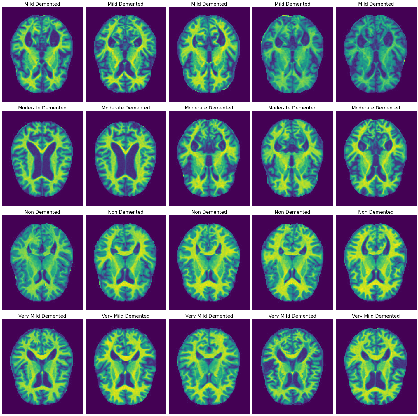
Figure 1: Sample Images of MRI Scans from the OASIS Dataset Representing Each Class of AD

In our work, we utilized the OASIS project that provides neuroimaging datasets of the brain to obtain the dataset. The study accessed cross-sectional MRI data from diverse age groups, including young and middle-aged individuals, as well as non-demented and demented older adults, using the OASIS-1 dataset. This dataset contains MRI scans of 416 male and female subjects ranging in age from 18 to 96. For each individual, it contains 3 to 4 T1-weighted-scans obtained from a single session. It also contains scans of non-demented subjects and subjects diagnosed with mild to moderate AD. Figure 1 showcases sample MRI scans from each Alzheimer’s class.

The OASIS dataset exhibited a high level of class imbalance, as evident from Table 1, with varying numbers of MRI scans across different types of AD (’MildDemented’, ’ModerateDemented’, ’NonDemented’, ’VeryMildDemented’). The number of images belongng to each type of AD has been tabulated in Table 1.

Table 1: Image Count of Each Type of Alzheimer’s Disease MRI Scans Before Augmentation

Type of Alzheimer’s Disease	Images Count
Non Demented	2560
Very Mild Demented	1792
Mild Demented	717
Moderate Demented	52

Addressing this imbalance is crucial for ensuring the proper learning of DL models. To mitigate this issue, the [22] Augmented Alzheimer MRI Dataset was utilized, which contains augmented images for each individual class of Alzheimer’s MRI scans. Through augmentation, this dataset achieves a more balanced distribution of images among all classes, effectively resolving the class imbalance problem. The distribution of images for each type of AD has been presented in Table 2.

Table 2: Image Count of Each Type of Alzheimer’s Disease MRI Scans After Augmentation

Type of Alzheimer’s Disease	Images Count
Non Demented	9600
Very Mild Demented	8960
Mild Demented	8960
Moderate Demented	6464

3.2 Methodology

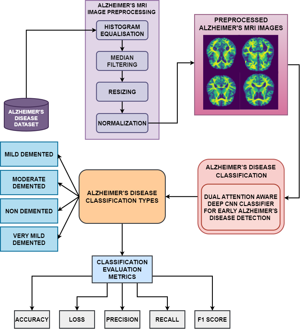
Figure 2: Overall Proposed System Workflow for Alzheimer’s Disease Classification

The augmented MRI images were first preprocessed using four preprocessing methods, namely histogram equalization, median filtering, image resizing, and pixel normalization. Histogram equalization improves the visual quality of the images, making it easier for the proposed DL classifier model to interpret them. Median filtering reduces the impact of noise without significantly blurring the edges of important structures. Resizing ensures that all images passed into the model have the same dimensions, which is necessary for batch processing and maintaining consistency across the dataset. Normalization helps the model converge faster during training by avoiding large input value ranges that can slow down learning. The preprocessed images were then used to train our proposed classifier model to classify the MRI images among one of the four AD types. We then evaluated the classification results using metrics such as F1-score, recall, accuracy, and precision. The flow of work has been depicted in Figure 2.

3.3 Preprocessing

We preprocessed the augmented images of the dataset using a pipeline comprising four stages: histogram equalization, median filtering, image resizing, and pixel normalization. Figure 5 illustrates the images at each stage of this preprocessing process applied to Alzheimer’s MRI images.

3.3.1 Histogram Equalization

Histogram equalization improves the contrast of an image by redistributing the pixel intensity levels. It can be difficult to distinguish between various tissues or structures in an MRI scan due to the vast range of intensity values that are frequently present in them. Histogram equalization works by spreading out the intensity values across the entire range of possible values.

$$\underbrace{I_{equalized}(x,y)}_{\text{Equalized Image}}=\underbrace{\left(\frac{L-1}{M\cdot N}\right)}_{\text{Scaling Factor}}\cdot\underbrace{\sum_{k=0}^{I_{in}(x,y)}\underbrace{H(k)}_{\text{Histogram}}}_{\text{Cumulative Distribution Function}}$$ (1)

By doing this, it enhances the contrast between different tissues or structures in the MRI scans, facilitating their identification and analysis. This is particularly useful in cases where the original MRI scan has poor contrast or where certain features are difficult to distinguish.

3.3.2 Median Filtering

AD MRI scans can be affected by the surrounding, causing the MRI scans to capture noise, such as Gaussian noise or salt-and-pepper noise, which can reduce the clarity of the images and make it more difficult to accurately analyze them. Median filtering operates by replacing every image pixel with the value of the median derived from the pixels surrounding it. In doing so, median filtering preserves the borders and details of the image’s structures while successfully eliminating noise-induced outliers. This enhances the general quality of MRI scans for AD, making it possible to extract features more accurately.

$$\underbrace{I_{out}(a,b)}_{\text{Output Image}}=\underbrace{\text{median}}_{\text{Median Operator}}\left(\underbrace{\{I_{in}(a+m,b+n)\mid m,n\in W\}}_{\text{Neighborhood Pixels}}\right)$$ (2)

3.3.3 MRI Image Resizing

Resizing helps prevent overfitting by reducing the complexity of the input data. DL models require a fixed input size, and resizing ensures that all images have the same dimensions when fed into the model. This is necessary for batch processing and maintaining consistency across the dataset. Resizing also speeds up the time it takes to train the model, which is important while working with large datasets as in this case.

$$\underbrace{I_{out}(u,v)}_{\text{Resized Image}}=\underbrace{\sum_{i=0}^{M-1}\sum_{j=0}^{N-1}\underbrace{I_{in}(i,j)}_{\text{Input Image}}\cdot\underbrace{K(u-S_{u}(i),v-S_{v}(j))}_{\text{Interpolation Kernel}}}_{\text{Interpolation Sum}}$$ (3)

3.3.4 Pixel Normalization

Pixel Normalization is done to transform the images’ pixel values between the range (0, 1). By minimizing wide input value ranges that can hinder learning, this preprocessing step assists in the model’s faster convergence during training. Gradient descent optimization algorithms in DL models perform better after normalizing input images because the gradients become more stable and less prone to vanishing. It also reduces overfitting by ensuring that the model learns patterns in the data rather than memorizing specific pixel values.

$$\underbrace{I_{norm}(i,j)}_{\text{Normalized Pixel}}=\frac{\underbrace{I(i,j)}_{\text{Pixel Value}}}{\underbrace{255.0}_{\text{Maximum Pixel Value}}}$$ (4)

The results following each preprocessing step of the Alzheimer’s MRI image have been shown in Figure 3.

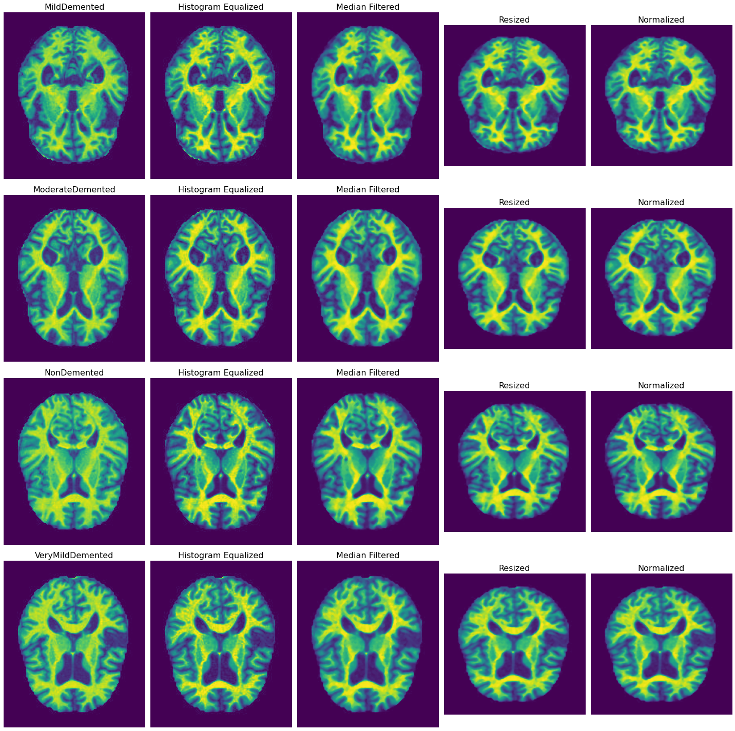
Figure 3: Alzheimer’s Disease MRI Scans Observed After Each Preprocessing Step

3.4 Proposed Dual-Attention Aware Deep Convolutional Neural Network

In this section, we present our proposed Spatial-Self Dual-Attention Aware CNN for Early Alzheimer’s Detection. The classifier is a unique DL model combining a combination of layers, each performing functions that are crucial for accurate classification of disease. Preprocessed MRI images were fed to the proposed model as input, which then outputs the predicted probabilities for these inputs. Figure 4 displays the architecture of our proposed classification model.

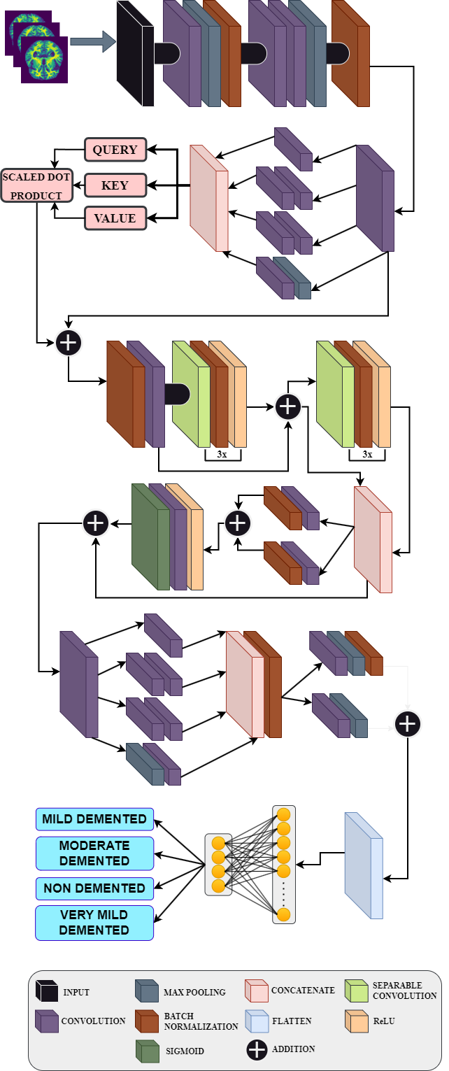
Figure 4: Proposed Dual-Attention Aware Deep CNN Layer Architecture for AD Classification

Our proposed model is designed to increase attention to detail in MRI scans and tackle the problem of vanishing gradients along layers. To enhance feature representation and enable efficient extraction of subtle details, we integrated both self-attention [23] and spatial attention [24] mechanisms into its architecture. Additionally, to overcome the challenge of vanishing gradients encountered during training, residual connections [25] were strategically embedded at various stages of feature extraction process. This enabled the model to precisely extract features and prioritize critical regions pivotal for distinguishing between different types of Alzheimer’s diseases, leading to a substantial enhancement in its overall performance.

The first convolutional block consists of a convolution layer that utilizes 64 filters with a 7x7 kernel size, which is then followed by a max-pooling layer. It serves as the model’s starting point, where it identifies basic visual elements like brain tissue boundaries and the overall brain structure layout, such as the contours of the hippocampus. Subsequently, the model employs batch normalization and additional convolutional layers with varying parameters, forming another convolutional block. This block further refines the initial features and helps in differentiating between gray and white matter, which is fundamental for recognizing the anatomical landmarks in the brain.

$$\underbrace{\text{Conv}(I_{(i,j)},F)}_{\text{Convolution Operation}}=\sum_{m=0}^{M-1}\sum_{n=0}^{N-1}\underbrace{I_{(i+m,j+n)}}_{\text{Input feature map}}\cdot\underbrace{F_{(m,n)}}_{\text{Filter}}+\underbrace{b}_{\text{Bias}}$$ (5)

$$\underbrace{\text{MaxPooling}(O)_{(i,j)}}_{\text{Max Pool Operation}}=\max_{p=0}^{k-1}\max_{q=0}^{k-1}\underbrace{I_{(i\cdot s+p,j\cdot s+q)}}_{\text{Input feature map}}$$ (6)

$$\underbrace{\text{BN}(x)}_{\text{Batch Normalization}}=\underbrace{\gamma}_{\text{Adaptable parameter}}\left(\frac{\underbrace{x}_{\text{Input}}-\underbrace{\mu}_{\text{Mean}}}{\sqrt{\underbrace{\sigma^{2}}_{\text{Variance}}+\underbrace{\epsilon}_{\text{constant}}}}\right)+\underbrace{\beta}_{\text{Adaptable parameter}}$$ (7)

This feature map is then fed to an inception block [26], where it significantly broadens its capacity to capture a wide range of features at different scales. It comprises parallel paths with convolutional layers of varying kernel sizes (5x5, 1x1, and 3x3) and a max-pooling path, enabling the model to extract detailed local features and broader contextual information simultaneously. It enables smaller kernels to zoom in on the intricate texture changes within the hippocampus, indicating potential neuronal loss. Meanwhile, larger kernels capture the overall enlargement of the ventricles, which is a common symptom in advanced Alzheimer’s cases. These parallel paths are finally concatenated to form the output feature vector from the inception block.

$$\underbrace{\text{concat}(X,Y)_{(p,q,r)}}_{\text{concatenation operation}}=\begin{cases}\underbrace{X_{(p,q,r)}}_{\text{input feature map from X}}&\text{if }1\leq r\leq\text{depth}(X)\\ \underbrace{Y_{(p,q,r-\text{depth}(X))}}_{\text{input feature map from Y}}&\text{if }\text{depth}(X)<r\leq\text{depth}(X)+\text{depth}(Y)\end{cases}$$ (8)

Following this, a self-attention mechanism is incorporated to dynamically evaluate the importance of different features within the MRI scans relative to each other. This enhances the model’s focus on regions that exhibit characteristic signs of AD, such as alterations in brain volume or the presence of neurofibrillary tangles and amyloid plaques. This self-attention mechanism recalibrates the focus on these vital features.

$$\underbrace{\alpha_{ij}}_{\text{Attention weight for position }(i,j)}=\underbrace{\text{softmax}\left(\frac{\underbrace{K^{T}Q}_{\text{Dot product of key and query}}}{\sqrt{\underbrace{d_{k}}_{\text{Dimensionality of key vectors}}}}\right)}_{\text{Softmax normalization}}\underbrace{V}_{\text{Value matrix}}$$ (9)

The feature map then flows through a series of separable convolution blocks with multiple residual connections to ensure proper flow of gradients along the network. Separable convolutional layers achieve efficient computation by splitting convolutions into depthwise and pointwise parts, minimizing computational complexity yet retaining the capacity to capture intricate spatial dependencies in MRI scans. Batch normalization stabilizes the learning process by normalizing layer activations, reducing internal covariate shifts. ReLU activation introduces nonlinearity, essential for modeling complex relationships between extracted features.

$$\underbrace{\text{ReLU}(x)}_{\text{Rectified Linear Unit Activation}}=\begin{cases}\underbrace{x}_{\text{Feature map}}&\text{if }x>0\\ 0&\text{otherwise}\end{cases}$$ (10)

After the series of separable convolutional blocks, the feature map undergoes a spatial attention mechanism. This mechanism highlights and magnifies crucial regions within the feature map’s spatial domain, such as altered cerebral blood flow patterns. This is followed by a second inception block, which complements the spatial attention mechanism by offering a comprehensive view of the MRI data at multiple resolutions.

Finally, a residual block is implemented, assisting the model to learn residual functions more effectively. This output is then flattened to a single dimension using a flattening layer, which is then processed through a dense layer. Finally, a softmax activation function delivers a probability distribution of the input MRI image over the different classes – ‘Mild Demented’, ‘Moderate Demented’, ‘Non-Demented’, and ‘Very Mild Demented’.

$$\underbrace{S(I_{i})}_{\text{Softmax Output}}=\frac{\underbrace{e^{I_{i}}}_{\text{Exponentiated Input}}}{\underbrace{\sum_{j=1}^{N}e^{I_{j}}}_{\text{Sum of Exponentiated Inputs}}}$$ (11)

The parameter specifications of the proposed Dual-Attention Aware Deep CNN are presented in Table 3.

Table 3: Proposed Model Parameter Specifications

Parameters	Coefficients
Total number of layers	68
Learning rate	0.001
Epochs	100
Batch size	128
Total Parameters	153,066,236

4 Results and Discussion

4.1 Experimental Setup

This section showcases the performance of the proposed model, alongside comparisons with other deep learning models. We carried out our experiments on a system characterized by the following specifications: Operating System - Linux 5.15.133; CPU - AMD EPYC 7763 with 128 CPU(s) and x86_64 architecture; GPU - AMD Radeon Instinct Model 1; with 64 Core(s) per socket, 2 Socket(s), and 1 Thread(s) per core. This information is summarized in Table 4.

Table 4: Configuration and Specifications of the System Used

Component	Specification
Operating System	Linux 5.15.133
CPU	AMD EPYC 7763
Architecture	x86_64
CPU(s)	128
GPU	AMD Radeon Instinct
Model	1
Core(s) per socket	64
Socket(s)	2
Thread(s) per core	1

4.2 Evaluation Metrics

Our proposed model’s performance for detecting AD was evaluated using the following metrics.

4.2.1 Accuracy

Accuracy can be defined as the evaluation metric which is responsible for determining how close the predicted value is to their true value. It is computed as a ratio between the count of true positives to the count of all the samples given to the model.

$$\underbrace{Accuracy}_{\text{Accuracy}}=\frac{\underbrace{\sum_{i=1}^{N}\underbrace{TP_{i}}_{\text{TruePositives}}+\underbrace{TN_{i}}_{\text{TrueNegatives}}}_{\text{CorrectPredictions}}}{\underbrace{N}_{\text{TotalSamples}}}$$ (12)

4.2.2 Recall

To measure the model’s performance which involves the capture ability of all the relevant instances, the recall metric is taken into account and is considered critical when there is an increase in the number of false negatives. It represents the proportion of true positives relative to the sum of true positives and false negatives.

$$\underbrace{Recall_{c}}_{\text{Recall for Class }c}=\frac{\underbrace{TP_{c}}_{\text{True Positives for Class }c}}{\underbrace{TP_{c}}_{\text{True Positives for Class }c}+\underbrace{FN_{c}}_{\text{False Negatives for Class }c}}$$ (13)

4.2.3 Precision

To measure the model’s performance which involves the identification ability of only the relevant instances, the precision metric is taken into account and is considered critical when there is an increase in the number of false positives. It denotes the ratio of true positives to the sum of true positives and false positives.

$$\underbrace{Precision_{c}}_{\text{Precision for Class }c}=\frac{\underbrace{TP_{c}}_{\text{True Positives for Class }c}}{\underbrace{TP_{c}}_{\text{True Positives for Class }c}+\underbrace{FP_{c}}_{\text{False Positives for Class }c}}$$ (14)

4.2.4 F1-Score

The F1-Score integrates precision and recall into a unified metric, providing a balanced assessment of the model’s performance. It is calculated as the harmonic mean of precision and recall.

$$\underbrace{\text{F1 Score}}_{\text{F1 Score for Class c}}=2\cdot\frac{\text{recall}\cdot\text{precision}}{\text{recall}+\text{precision}}$$ (15)

Our classifier was trained for 100 epochs, and the performance metrics obtained at every epoch are recorded and plotted against each epoch to observe the variation in the model performance compared to its previous iterations. The scores obtained for accuracy, recall, precision, and F1-score are illustrated in Figures 5, 8, 7, and 9 respectively. The categorical cross entropy loss function was utilized to determine the loss incurred during training, and the obtained loss at each epoch is illustrated in Figure 6.

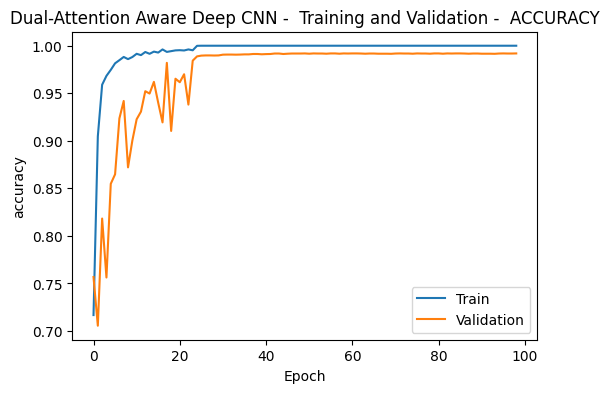
Figure 5: Training and validation accuracy plots for the Proposed Model

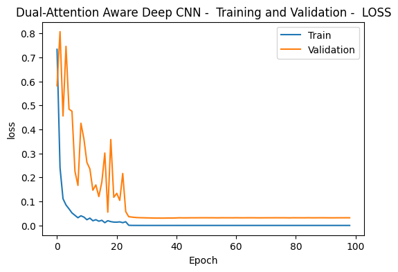
Figure 6: Training and validation loss plots for the Proposed Model

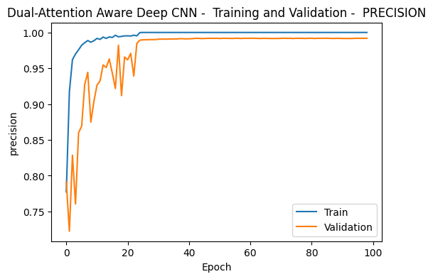
Figure 7: Training and validation precision plots for the Proposed Model

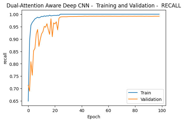
Figure 8: Training and validation recall plots for the Proposed Model

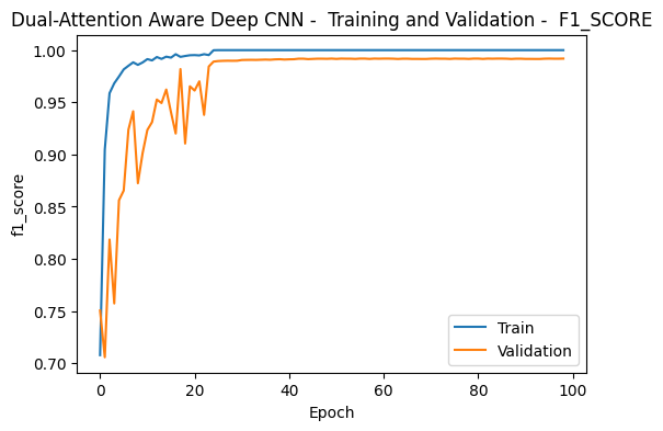
Figure 9: Training and validation F1-score plots for the Proposed Model

The above graphs show that our proposed model has demonstrated robust and exceptional performance during its learning phase. The model learns most of the features effectively up to around 30 epochs, after which it starts to converge. The proposed model achieved a precision of 99.3%, a recall of 99.6%, an F1-score of 99.3%, and an accuracy of 99.2%. These metrics indicate that the proposed model has learned the data well while being able to apply it to unseen scenarios effectively as seen from the validation curve. The self and spatial dual-attention mechanisms integrated into the model allow it to effectively extract spatial dependencies from the MRI images, while also being able to apply more focus to specific parts of the image by comparing various aspects of the same image.

4.2.5 Discussions

The confusion matrix for the testing data using our trained proposed model is shown in Figure 10. This type of matrix displays values as proportions or percentages, making it easy to compare classification performance across different classes. With values ranging from 0 to 1, it simplifies interpretation. The matrix illustrates the classifier’s performance for the four AD classes: "Mild Demented," "Moderate Demented," "Non-Demented," and "Very Mild Demented." Each column represents the predicted class, while each row represents the actual (True) class. The main diagonal values indicate the percentage of correctly classified cases, whereas the off-diagonal values represent misclassified cases.

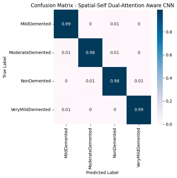
Figure 10: Confusion Matrix Obtained from the Proposed Model

It can be observed from the confusion matrix that our model has impressive accuracy across all classes. The majority of samples were correctly classified as shown by values close to one along the diagonal. For instance, for “Mild Demented” class, the model yielded a 0.99 true positive rate (TPR), implying that 99% of samples were correctly classified. Again, for “Moderate Demented” class, had a TPR of 0.98 showing that 98% of cases were correctly classified. The ‘Non-Demented’ class also had a high TPR of 0.98 expressing correct classification at 98%. Lastly, the “Very Mild Demented” class had a 0.99 TPR, indicating that there was an accurate identification of about 99% of samples in this category. In conclusion, these levels of misclassification rates indicated how effective these models are in differentiating various stages of Alzheimer’s ailment because they have small values off-diagonal.

Our proposed model was evaluated against other SOTA CNNs - DenseNet121 [27], EfficientNetV2 [28], InceptionV3 [26], InceptionResNetV2 [29], MobileNetV2 [30], MobileNet [31], NASNetMobile [32], ResNet50 [25], VGG16 [33], and Xception [34]. The comparison aimed to assess our model against established CNN benchmarks used as baselines for AD detection. The models were trained using the augmented OASIS dataset, and the results have been tabulated in Table 5. Evaluation of these models was based on key metrics such as Precision (Prec), Accuracy (Acc), F1-score (F1), and Recall (Rec).

Table 5: Proposed model performance comparison against pretrained CNNs during Training and Validation Phase

Model	Training Phase Metrics				Validation Phase Metrics
	Accuracy	Precision	Recall	F1	Accuracy	Precision	Recall	F1
DenseNet121	0.991	0.991	0.992	0.991	0.951	0.962	0.961	0.962
EfficientNetV2	0.990	0.991	0.992	0.991	0.931	0.942	0.931	0.931
InceptionV3	0.992	0.991	0.992	0.991	0.961	0.961	0.971	0.961
InceptionResNetV2	0.951	0.951	0.962	0.961	0.932	0.942	0.931	0.931
MobileNetV2	0.981	0.982	0.981	0.982	0.891	0.901	0.911	0.901
MobileNet	0.971	0.981	0.972	0.981	0.891	0.901	0.901	0.901
NASNetMobile	0.992	0.992	0.991	0.992	0.891	0.881	0.882	0.882
ResNet50	0.991	0.981	0.981	0.981	0.921	0.911	0.911	0.911
VGG16	0.881	0.891	0.881	0.881	0.781	0.791	0.781	0.781
Xception	0.991	0.991	0.992	0.991	0.961	0.952	0.961	0.961
Proposed CNN	0.992	0.991	0.991	0.992	0.991	0.992	0.995	0.993

From Table 5, we can infer that our proposed model has performed significantly well compared to other baseline CNN-based models. DenseNet121 benefits from dense connectivity, which aids in feature reusing; however, it impacts its ability to accurately identify particular Alzheimer’s features such as amyloid plaques and neurofibrillary tangles. EfficientNetV2 tends to overfit, due to challenges in capturing the subtle features of AD, such as the minor changes in brain structure or variations in brain activity observed in MRI scans. InceptionV3 is designed for efficient computation, making it incapable of analyzing the multidimensional characteristics of Alzheimer’s MRI data, especially in detecting subtle neural network disruptions or changes in brain volume. Despite its complicated structure, there is an inadequate match between InceptionResNetV2 and the demand to distinguish precise disease-specific features such as synaptic loss or alterations in brain function.

The lightweight design of MobileNetV2 is not as good at detailed analysis to identify conditions like the early symptoms of AD, that is, mild cognitive impairment (MCI) or minor hippocampal atrophy. By focusing on efficiency, MobileNet sacrifices the depth needed for thorough feature extraction from Alzheimer’s MRI images. The NASNetMobile, designed for mobile applications, is not fine-tuned enough to capture all the significant intersections that would signal Alzheimer’s such as altered white matter integrity or cortical atrophy. ResNet50’s depth and focus may make it difficult to learn about such things as hippocampal atrophy. Simplicity and the relative shallowness of VGG16 struggle with such detailed analysis where ventricular enlargement is observed resulting in low validation accuracy tests. Xception does not fully exploit the spatial relationships that are key to identifying specific indicators of Alzheimer’s, like brain atrophy patterns or connectivity between brain regions. Our proposed model stands out given that it combines dual spatial and self-attention mechanisms, providing a unique ability to identify amyloid deposition, neural network disruptions, and hippocampal atrophy among other critical features. These improvements assist in capturing intricate and heterogeneous pathology patterns typical for AD as seen from MRI scans.

Our model was also compared with existing research in the area of AD detection using ML and DL. The comparison of performance between these models is detailed in Table 6.

Table 6: Proposed model performance metrics comparison with existing research

Model	Accuracy (%)	Recall (%)	F1 (%)	Precision (%)
CNN, RNN, LSTM Ensemble [19]	89.75	91.07	89.08	89.16
CNN, RNN, LSTM Bagged Ensemble [19]	92.22	92.57	91.87	91.92
Wavelet Entropy, MLP and BBO [35]	92.41	92.47	92.3	92.14
DEMNET without SMOTE [36]	85.43	88.32	83.32	80.11
DEMNET with SMOTE [36]	95.23	95.21	95.27	96.43
Proposed Method	99.12	99.54	99.31	99.21

From Table 6, we can infer that the CNN, RNN, and LSTM Ensemble model attained an accuracy of 89.75%, with recall, precision, and F1 scores of 91.07%, 89.16%, and 89.08%, respectively. The CNN, RNN, and LSTM Bagged Ensemble showed a slight improvement, with precision of 91.92%, accuracy of 92.22%, F1 score of 91.87%, and recall of 92.57%. The Wavelet Entropy, Multilayer Perceptron, and Biogeography-Based Optimization model performed comparably, achieving an accuracy of 92.4%, precision of 92.14%, recall of 92.47%, and an F1 score of 92.3%.

DEMNET without SMOTE had the lowest performance among the compared models, with a recall of 88.32%, precision of 80.11%, an F1 score of 83.32%, and an accuracy of 85.43%. However, when SMOTE was applied to DEMNET, the model’s performance significantly improved, achieving a recall of 95.21%, precision of 96.43%, an F1 score of 95.27%, and an accuracy of 95.23%,. Our proposed methodology demonstrates notable performance, with a recall of 99.54%, precision of 99.21%, F1 score of 99.31%, and an accuracy of 99.12%. This success can be attributed to its advanced feature extraction capabilities, effectively identifying critical biomarkers such as hippocampal atrophy and cortical thinning. These advancements enable the model to effectively capture the subtle and complex patterns associated with AD, leading to more accurate detection.

5 Conclusion and Future Scope

AD is widely observed to be one of the irreversible degenerative disorders, that progresses slowly and leads to serious complications like neuronal cell death. By leveraging a dual spatial and self-attention based CNN model, we proposed a novel classification approach for the detection of AD, offering promising prospects for early detection and improved diagnostic outcomes. The high accuracy and precision scores of our proposed model indicate its robustness and reliability in identifying and classifying AD. Future research can explore the integration of Graph Neural Networks (GNNs) and Graph Attention Networks (GATs) to further enhance model performance. By utilizing the capabilities of GATs and GNNs, we can capture complex relationships and dependencies within neuroimaging data by utilizing inter-regional and intra-regional connections. Additionally, utlilizing larger and more diverse datasets will help refine these models, leading to improved accuracy and generalization. This advancement holds promise not only for improving Alzheimer’s diagnosis but also for application in the broader field of neurodegenerative disease research.

References

- [1] H.-I. Suk, S.-W. Lee, and D. Shen, “Hierarchical feature representation and multimodal fusion with deep learning for ad/mci diagnosis,” NeuroImage, vol. 101, pp. 569–582, 2014.
- [2] T. Jo, K. Nho, S. L. Risacher, and A. J. Saykin, “Deep learning detection of informative features in tau pet for alzheimer’s disease classification,” BMC Bioinformatics, vol. 21, no. S21, 2020.
- [3] S. Liu, S. Liu, W. Cai, S. Pujol, R. Kikinis, and D. Feng, “Early diagnosis of alzheimer’s disease with deep learning,” in 2014 IEEE 11th International Symposium on Biomedical Imaging (ISBI). IEEE, 2014, pp. 1015–1018.
- [4] S. Spasov, L. Passamonti, A. Duggento, P. Liò, and N. Toschi, “A parameter-efficient deep learning approach to predict conversion from mild cognitive impairment to alzheimer’s disease,” NeuroImage, 2019.
- [5] T. Jo, K. Nho, and A. J. Saykin, “Deep learning in alzheimer’s disease: Diagnostic classification and prognostic prediction using neuroimaging data,” Frontiers in Aging Neuroscience, vol. 11, 2019.
- [6] D. S. Marcus, T. H. Wang, J. Parker, J. G. Csernansky, J. C. Morris, and R. L. Buckner, “Open access series of imaging studies (oasis): Cross-sectional mri data in young, middle aged, nondemented, and demented older adults,” Journal of Cognitive Neuroscience, vol. 19, no. 9, pp. 1498–1507, sep 2007. [Online]. Available: http://dx.doi.org/10.1162/jocn.2007.19.9.1498
- [7] H. A. Helaly, M. Badawy, and A. Y. Haikal, “Deep learning approach for early detection of alzheimer’s disease,” Cognitive Computation, vol. 14, no. 5, pp. 1711–1727, nov 2021. [Online]. Available: http://dx.doi.org/10.1007/s12559-021-09946-2
- [8] J. Venugopalan, L. Tong, H. R. Hassanzadeh, and M. D. Wang, “Multimodal deep learning models for early detection of alzheimer’s disease stage,” Scientific Reports, vol. 11, no. 1, feb 2021. [Online]. Available: http://dx.doi.org/10.1038/s41598-020-74399-w
- [9] A. A, P. M, M. Hamdi, S. Bourouis, R. Kulhanek, and F. Mohmed, “Evaluation of neuro images for the diagnosis of alzheimer’s disease using deep learning neural network,” Frontiers in Public Health, vol. 10, feb 2022. [Online]. Available: http://dx.doi.org/10.3389/fpubh.2022.834032
- [10] A. Puente-Castro, E. Fernandez-Blanco, A. Pazos, and C. R. Munteanu, “Automatic assessment of alzheimer’s disease diagnosis based on deep learning techniques,” Computers in Biology and Medicine, vol. 120, p. 103764, may 2020. [Online]. Available: http://dx.doi.org/10.1016/j.compbiomed.2020.103764
- [11] F. Zhang, B. Pan, P. Shao, P. Liu, S. Shen, P. Yao, and R. X. Xu, “A single model deep learning approach for alzheimer’s disease diagnosis,” Neuroscience, vol. 491, pp. 200–214, 2022. [Online]. Available: https://www.sciencedirect.com/science/article/pii/S030645222200149X
- [12] L. Liu, S. Zhao, H. Chen, and A. Wang, “A new machine learning method for identifying alzheimer’s disease,” Simulation Modelling Practice and Theory, vol. 99, p. 102023, feb 2020. [Online]. Available: http://dx.doi.org/10.1016/j.simpat.2019.102023
- [13] C.-H. Chang, C.-H. Lin, and H.-Y. Lane, “Machine learning and novel biomarkers for the diagnosis of alzheimer’s disease,” International Journal of Molecular Sciences, vol. 22, no. 5, p. 2761, mar 2021. [Online]. Available: http://dx.doi.org/10.3390/ijms22052761
- [14] M. A. Ebrahimighahnavieh, S. Luo, and R. Chiong, “Deep learning to detect alzheimer’s disease from neuroimaging: A systematic literature review,” Computer Methods and Programs in Biomedicine, vol. 187, p. 105242, apr 2020. [Online]. Available: http://dx.doi.org/10.1016/j.cmpb.2019.105242
- [15] H. Ji, Z. Liu, W. Q. Yan, and R. Klette, “Early diagnosis of alzheimer’s disease using deep learning,” in Proceedings of the 2nd International Conference on Control and Computer Vision (ICCCV 2019). ACM, jun 2019. [Online]. Available: http://dx.doi.org/10.1145/3341016.3341024
- [16] A. Khan and S. Zubair, “An improved multi-modal based machine learning approach for the prognosis of alzheimer’s disease,” Journal of King Saud University – Computer and Information Sciences, 2020.
- [17] M. Orouskhani, C. Zhu, S. Rostamian, F. Shomal Zadeh, M. Shafiei, and Y. Orouskhani, “Alzheimer’s disease detection from structural mri using conditional deep triplet network,” Neuroscience Informatics, 2020.
- [18] A. W. Saleh and G. Gupta, “An alzheimer’s disease classification model using transfer learning densenet with embedded healthcare decision support system,” Decision Analytics Journal, 2020.
- [19] M. Dua and D. Makhija, “A cnn–rnn–lstm based amalgamation for alzheimer’s disease detection,” Journal of Medical and Biological Engineering, 2020.
- [20] C. L. Saratxaga and I. Moya, “Mri deep learning-based solution for alzheimer’s disease prediction,” Journal of Personalized Medicine, 2020.
- [21] J. Liu and Y. Luo, “Alzheimer’s disease detection using depthwise separable convolutional neural networks,” 2020.
- [22] Uraninjo, “Augmented alzheimer mri dataset,” https://www.kaggle.com/datasets/uraninjo/augmented-alzheimer-mri-dataset/data, 2024.
- [23] A. Vaswani, N. Shazeer, N. Parmar, J. Uszkoreit, L. Jones, A. N. Gomez, L. Kaiser, and I. Polosukhin, “Attention is all you need,” Advances in neural information processing systems, vol. 30, 2017.
- [24] S. Woo, J. Park, J.-Y. Lee, and I. S. Kweon, “Cbam: Convolutional block attention module,” in Proceedings of the European conference on computer vision (ECCV), 2018, pp. 3–19.
- [25] K. He, X. Zhang, S. Ren, and J. Sun, “Deep residual learning for image recognition,” in Proceedings of the IEEE conference on computer vision and pattern recognition, 2016, pp. 770–778.
- [26] C. Szegedy, W. Liu, Y. Jia, P. Sermanet, S. Reed, D. Anguelov, D. Erhan, V. Vanhoucke, and A. Rabinovich, “Going deeper with convolutions,” in Proceedings of the IEEE conference on computer vision and pattern recognition, 2015, pp. 1–9.
- [27] G. Huang, Z. Liu, and K. Q. Weinberger, “Densely connected convolutional networks,” CoRR, vol. abs/1608.06993, 2016. [Online]. Available: http://arxiv.org/abs/1608.06993
- [28] M. Tan and Q. V. Le, “Efficientnetv2: Smaller models and faster training,” CoRR, vol. abs/2104.00298, 2021. [Online]. Available: https://arxiv.org/abs/2104.00298
- [29] C. Szegedy, S. Ioffe, and V. Vanhoucke, “Inception-v4, inception-resnet and the impact of residual connections on learning,” CoRR, vol. abs/1602.07261, 2016. [Online]. Available: http://arxiv.org/abs/1602.07261
- [30] M. Sandler, A. G. Howard, M. Zhu, A. Zhmoginov, and L.-C. Chen, “Inverted residuals and linear bottlenecks: Mobile networks for classification, detection and segmentation,” CoRR, vol. abs/1801.04381, 2018. [Online]. Available: http://arxiv.org/abs/1801.04381
- [31] A. G. Howard, M. Zhu, B. Chen, D. Kalenichenko, W. Wang, T. Weyand, M. Andreetto, and H. Adam, “Mobilenets: Efficient convolutional neural networks for mobile vision applications,” CoRR, vol. abs/1704.04861, 2017. [Online]. Available: http://arxiv.org/abs/1704.04861
- [32] B. Zoph, V. Vasudevan, J. Shlens, and Q. V. Le, “Learning transferable architectures for scalable image recognition,” CoRR, vol. abs/1707.07012, 2017. [Online]. Available: http://arxiv.org/abs/1707.07012
- [33] K. Simonyan and A. Zisserman, “Very deep convolutional networks for large-scale image recognition,” arXiv preprint arXiv:1409.1556, 2015. [Online]. Available: http://arxiv.org/abs/1409.1556
- [34] F. Chollet, “Xception: Deep learning with depthwise separable convolutions,” CoRR, vol. abs/1610.02357, 2016. [Online]. Available: http://arxiv.org/abs/1610.02357
- [35] S. Wang, Y. Zhang, Y. Li et al., “Single slice based detection for alzheimer’s disease via wavelet entropy and multilayer perceptron trained by biogeography-based optimization,” Multimedia Tools and Applications, vol. 77, pp. 10 393–10 417, 2018.
- [36] S. Murugan, C. Venkatesan, M. G. Sumithra, X.-Z. Gao, B. Elakkiya, M. Akila, and S. Manoharan, “Demnet: A deep learning model for early diagnosis of alzheimer diseases and dementia from mr images,” IEEE Access, vol. 9, pp. 90 319–90 329, 2021.