High precision calculation of the hadronic vacuum polarisation contribution to the muon anomaly

A. Boccaletti^1,2, Sz. Borsanyi¹, M. Davier³, Z. Fodor^{1,4,5,2,6,7,∗}, F. Frech¹, A. Gérardin⁸, D. Giusti^2,9, A.Yu. Kotov², L. Lellouch⁸, Th. Lippert², A. Lupo⁸, B. Malaescu¹⁰, S. Mutzel^8,11, A. Portelli^12,13, A. Risch¹, M. Sjö⁸, F. Stokes^2,14, K.K. Szabo^1,2, B.C. Toth¹, G. Wang⁸, Z. Zhang³

¹ Department of Physics, University of Wuppertal, D-42119 Wuppertal, Germany
² Jülich Supercomputing Centre, Forschungszentrum Jülich, D-52428 Jülich, Germany
³ IJCLab, Université Paris-Saclay et CNRS/IN2P3, Orsay, 91405, France
⁴ Physics Department, Pennsylvania State University, University Park, PA 16802, USA
⁵ Institute for Computational and Data Sciences, Pennsylvania State University, University Park, PA 16802, USA
⁶ Institute for Theoretical Physics, Eötvös University, H-1117 Budapest, Hungary
⁷ University of California, San Diego, 9500 Gilman Drive, La Jolla, CA 92093, USA
⁸ Aix Marseille Univ, Université de Toulon, CNRS, CPT, IPhU, Marseille, France
⁹ Fakultät für Physik, Universität Regensburg, 93040, Regensburg, Germany
¹⁰ LPNHE, Sorbonne Université, Université Paris Cité, CNRS/IN2P3, Paris, 75252, France
¹¹ Laboratoire de Physique de l’Ecole Normale Supérieure, Mines Paris - PSL, CNRS, Inria, PSL Research University, Paris, France
¹² School of Physics and Astronomy, University of Edinburgh, Edinburgh EH9 3JZ, United Kingdom
¹³ RIKEN Center for Computational Science, Kobe 650-0047, Japan
¹⁴ Special Research Centre for the Subatomic Structure of Matter, Department of Physics University of Adelaide, South Australia 5005, Australia

For fifty years, the standard model of particle physics has been hugely successful in describing subatomic phenomena. Recently, this statement appeared to be contradicted by the strong disagreement between measurements of the anomalous magnetic moment of the muon [116], $a_{\mu}$, and the reference standard-model prediction [115]. Such a large discrepancy should signal the discovery of interactions or particles not present in the standard model. However, two independent determinations [52, 105] of the most uncertain contribution to the standard-model prediction display significantly less tension with the measurement. Here we present a new first-principle calculation of this contribution. We reduce uncertainties compared to our earlier computation [52] by $40\%$. To reach this unprecedented level of precision we improve on many aspects of the calculation. Namely, we perform large-scale lattice QCD simulations on finer lattices than in Ref. [52], allowing for an even more accurate continuum extrapolation. We also include a small, long-distance contribution obtained using input from experiments in a low-energy regime where they all agree. Combined with the extensive calculations of other standard model contributions summarised in Ref. [115], our result leads to a prediction that differs from the measurement of $a_{\mu}$ by only 0.9 standard deviations. This provides a remarkable validation of the standard model to 0.37ppm.

The muon is a short-lived elementary particle with spin 1/2 and with a mass 207 times larger than that of the electron. Both particles create a magnetic field around them characterised by a magnetic dipole moment. This moment is proportional to the spin and charge of the particle, and inversely proportional to twice its mass. Dirac’s relativistic quantum mechanics predicts that the constant of proportionality, $g_{\mu}$, known as the Landé factor, is precisely 2. Relativistic quantum field theory leads to additional small corrections, to which all particles and interactions of the standard model (SM) contribute. Because muons are more massive than electrons, quantum corrections associated with massive particles are generically much larger for the muon than for the electron [5]. This increased sensitivity to the effects of possible unknown particles is the reason for the current focus on the muon. The corrections to $g_{\mu}$ are commonly called the anomalous magnetic moment and are quantified as $a_{\mu}=(g_{\mu}-2)/2$.

When calculating $a_{\mu}$ the uncertainty comes almost exclusively from the strong interaction, described in the SM by quantum chromodynamics (QCD). In particular, the dominant source of uncertainty comes from hadronic vacuum polarisation at leading order in the fine-structure constant (LO-HVP). More generally, HVP induces a modification in the propagation of a virtual photon in the vacuum, caused by the strong interaction.

Here we present a calculation of this LO-HVP contribution to $a_{\mu}$ ($a_{\mu}^{\text{LO-HVP}}$) with unprecedented accuracy. To that end we apply numerical lattice quantum field theory techniques that allow to make QCD predictions in the highly nonlinear regime that is relevant here. QCD is a generalised version of quantum electrodynamics (QED) that describes the strong interaction instead of the electromagnetic one. The Euclidean Lagrangian for a quark of mass $m$ and charge $q$ (in units of the positron charge, $e$), subject to strong and electromagnetic interactions, can be written as ${\cal L}=-1/(4e^{2})F_{\mu\nu}F_{\mu\nu}-1/(2g^{2})\,\mathrm{Tr}\,G_{\mu\nu}G_{\mu\nu}+{\bar{\psi}}[\gamma_{\mu}(\partial_{\mu}+qA_{\mu}+G_{\mu})+m]\psi$, where $F_{\mu\nu}=\partial_{\mu}A_{\nu}-\partial_{\nu}A_{\mu}$, $G_{\mu\nu}=\partial_{\mu}G_{\nu}-\partial_{\nu}G_{\mu}+[G_{\mu},G_{\nu}]$ and $g$ is the QCD coupling constant. The fermionic quark fields $\psi$ have an additional “colour” index in QCD, which runs from 1 to 3. Different “flavours” of quarks are represented by independent fermionic fields, with different masses and charges. In QED, the gauge potential $A_{\mu}$ is a real valued field, whereas in QCD, $G_{\mu}$ is a 3$\times$3 matrix field acting in “colour” space. In the present work we include both QCD and QED as well as four nondegenerate quark flavours (up, down, strange and charm) in a fully-dynamical, staggered-fermion formulation. We also consider the tiny contributions of the bottom and top quarks. Their errors are subdominant, and we repeat the treatment of our earlier analysis [52].

To calculate the LO-HVP contribution to $a_{\mu}$, we start with the zero-three-momentum two-point function of the quark electromagnetic current in Euclidean time $t$ [125]. In this so-called time-momentum representation, it is given by

$$G(t)=-\frac{1}{3e^{2}}\sum_{\mu=1,2,3}\int d^{3}x\langle J_{\mu}(\vec{x},t)J_{\mu}(0)\rangle\ ,$$ (1)

where $J_{\mu}$ is the quark electromagnetic current with $J_{\mu}/e=\frac{2}{3}\bar{u}\gamma_{\mu}u-\frac{1}{3}\bar{d}\gamma_{\mu}d-\frac{1}{3}\bar{s}\gamma_{\mu}s+\frac{2}{3}\bar{c}\gamma_{\mu}c$. $u,d,s$ and $c$ are the up, down, strange and charm quark fields and the angle brackets stand for the QCD+QED expectation value to order $e^{2}$. It is convenient to decompose $G(t)$ into light ($u$ and $d$), strange, charm and disconnected components, which have very different statistical and systematic uncertainties. Performing a weighted integral of the one-photon-irreducible part, $G_{\mathrm{1\gamma I}}(t)$, of $G(t)$ from $t=0$ to infinity yields the LO-HVP contribution to $a_{\mu}$ [125]. The weight is a known kinematic function, $K(tm_{\mu})$ [7, 8, 9, 125]. Thus:

$$a_{\mu}^{\mathrm{LO-HVP}}=\alpha^{2}\int_{0}^{\infty}dt\ K(tm_{\mu})\ G_{\mathrm{1\gamma I}}(t)\ ,$$ (2)

where $\alpha$ is the fine-structure constant at vanishing recoil and $m_{\mu}$ is the mass of the muon.

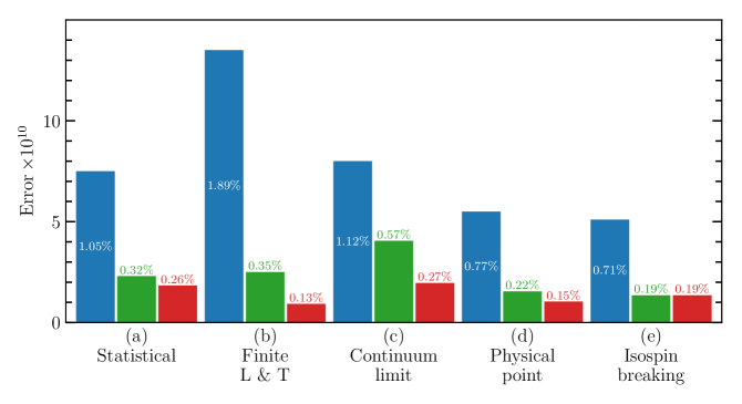
Figure 1: Main uncertainties and their reduction in our successive lattice calculations of $a_{\mu}^{\text{LO-HVP}}$. Their sources are labelled (a-e) in the text and are given a short descriptive title below the bars in the plot. Their approximate size relative to the total LO-HVP contribution obtained in the present work is also shown. The blue bars on the left of each group correspond to our 2017 result [78], the green ones in the middle to our 2020 findings [52] and the red ones on the right to the work presented here.

Reducing the uncertainty in the calculation of $a_{\mu}^{\text{LO-HVP}}$ to below half a percent is a major challenge. In particular, a number of contributions to this uncertainty must be controlled. They are (a) statistical uncertainties; (b) those associated with the finite spatial size $L$ and time $T$ of the lattice; (c) with the extrapolation to the continuum limit; (d) with fixing the five parameters of four-flavour QCD; (e) with QED and strong-isospin breaking (SIB) corrections. The progress made in our successive lattice calculations of $a_{\mu}^{\text{LO-HVP}}$ is illustrated in Fig. 1, where those contributions to the uncertainty are shown. In the present work we have focused on reducing the two largest ones in our 2020 calculation, which are (c) and (b). We discuss these uncertainties in detail now.

ad (a). Statistical uncertainties in the light-quark-connected and disconnected contributions to the correlation function of Eq. (1), associated with the stochastic evaluation of the QCD and QED path integrals, increase exponentially at large Euclidean times $t$. In addition to the many improvements made in [52], to reduce those uncertainties further we used mock analyses to determine which ensembles required more statistics. In particular, we increased the statistics on the lattices which have the smallest lattice spacings and which are critical for controlling the necessary continuum extrapolations. Moreover, to control the statistical uncertainties at large $t$ we replaced the lattice calculation of the contribution to $a_{\mu}^{\text{LO-HVP}}$ from $G(t)$ above $t\geq 2.8\,\mathrm{fm}$ by a state-of-the-art, data-driven determination, via the HVPTools setup [122, 123, 124, 102]. Before combining the two results, we verified that the lattice and the data-driven determinations of part of this long-distance “tail” contribution (based on measurements of the hadron spectrum in $e^{+}e^{-}$ annihilation and $\tau$-decay experiments) agree within errors. We computed this tail contribution using the most precise measurements of the two-pion spectrum by BaBar [103, 104], KLOE [106, 107, 108, 109] and CMD-3 [105], as well as the one obtained from hadronic $\tau$ decays [119, 120]. Those spectra are supplemented by the contributions from all of the other hadronic final states, as described in Ref. [118]. The tail contribution is dominated by centre-of-mass energies below the $\rho$-meson peak, a region where all the measurements agree very well. Moreover, it only accounts for less than $5\%$ of our final, lattice-dominated result for $a_{\mu}^{\text{LO-HVP}}$, but is responsible for roughly $65\%$ of the square of the $2.2\times 10^{-10}$ reduction on the total error compared to our 2020 calculation. The Supplementary Information describes our determination of this contribution and further justifies its use in our calculation.

ad (b). Finite $L$ and $T$ corrections gave the largest contribution to the error in 2017 [78]. Even in our 2020 calculation [52] it was still a significant source of uncertainty. Here our determination of the tail contribution using a data-driven approach reduces those corrections by a factor of about two and the associated uncertainties by even more. We compute those corrections using the dedicated simulations of Ref. [52], supplemented by NNLO chiral perturbation theory for distances beyond $11\,\mathrm{fm}$ [52, 92]. Those results are checked against nonperturbative analytical approaches to finite-volume corrections [94, 96, 95, 97, 98] that we complement with experimental $\pi^{+}\pi^{-}$ cross-section data below $1.3\,\mathrm{Ge\kern-1.00006ptV}$. Details are given in the Supplementary Information.

ad (c). The continuum extrapolation of the isovector contribution to $a_{\mu}^{\text{LO-HVP}}$ was the largest source of uncertainty in our 2020 computation [52] and we have dedicated significant resources to further control it. The uncertainties were mainly due to long-distance, taste-breaking effects that are present in staggered-fermion computations. Here we have added a new, finer lattice spacing. The corresponding simulations have a numerical cost close to the one required for the full 2020 computation. In Ref. [52] the smallest lattice spacing was $0.064\,\mathrm{fm}$. The new lattice spacing is $0.048\,\mathrm{fm}$. Since the leading discretisation effects are proportional to the square of the lattice spacing, results at this new lattice spacing have cutoff effects reduced by a factor of nearly two. We further account for the fact that different $t$-regions in $G(t)$ have different cut-off effects by dividing the integral of Eq. (2) into four $t$ intervals delimited by sigmoid functions. Such intervals or “windows” were first proposed in Ref. [79]. The first of our windows corresponds to the Euclidean-time interval $0.0$ to $0.4\,\mathrm{fm}$, known as the short-distance (SD) window [115, 79] and denoted $a_{\mu,00-04}^{\text{LO-HVP}}$ here. We use three more intervals between $0.4$ and $2.8\,\mathrm{fm}$ (separated at $0.6$ and $1.2\,\mathrm{fm}$) because this choice yields a reduced uncertainty on the final result for $a_{\mu}^{\text{LO-HVP}}$. We carry out the continuum extrapolation in those windows separately. We then add the individual extrapolated results to obtain the contribution to $a_{\mu}^{\text{LO-HVP}}$ from the Euclidean time interval from $0$ to $2.8\,\mathrm{fm}$, taking correlations into account. The new ensembles are responsible for roughly $2/3$ of the reduction in the continuum-extrapolation uncertainty on $a_{\mu}^{\text{LO-HVP}}$ compared to our 2020 computation, with the remaining $1/3$ coming from the fact that we use a data-driven approach to compute the tail contribution, as discussed above. This whole procedure is detailed in the Supplementary Information.

ad (d). We improve the determination of the physical point, which we base on a very precise computation of the mass of the $\Omega^{-}$ baryon. The uncertainty associated with this determination was already small in Ref. [52] and is even smaller here. For details see the Supplementary Information.

ad (e). The QED and SIB uncertainties obtained in Ref. [52] are already sufficiently small to reach the precision sought here. Here we have performed a variety of crosschecks that confirm those earlier results. Details are given in the Supplementary Information.

By far the largest contributions to the various windows considered in this work come from connected light-quark diagrams. We focus on these here and discuss the other contributions in the Supplementary Information.

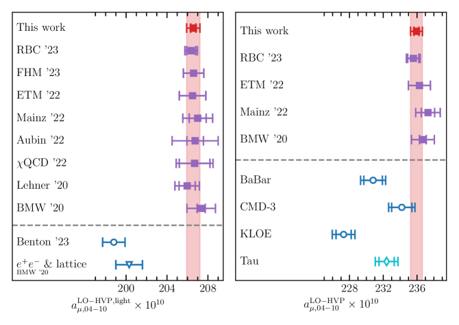
Figure 2: Left panel: comparison of our result for the light contribution of the intermediate-distance window, $a_{\mu,04-10}^{\text{LO-HVP},\mathrm{light}}$, with other results in the literature. Our result is the red square, the purple squares correspond to other lattice computations, the blue circle [89] and triangle [52] to data-driven approaches. Right panel: comparison of determinations of the full $a_{\mu,04-10}^{\text{LO-HVP}}$. Here, in the data-driven case, we show results [118] that use the measurements of the two-pion spectrum obtained in individual electron-positron annihilation experiments and in $\tau$-decays, as explained in Ref. [118]. The references for the lattice results in the left panel and for the experimental spectra used to obtain the results in the right panel are given in the text. The error bars correspond to the standard error of the mean (SEM).

For the connected contribution of the light $u$ and $d$ quarks to the SD window we find $a_{\mu,00-04}^{\text{LO-HVP},\mathrm{light}}=47.84(4)(15)[15]\times 10^{-10}$ and to the ID window, $a_{\mu,04-10}^{\text{LO-HVP},\mathrm{light}}=206.57(25)(60)[65]\times 10^{-10}$, with statistical, systematic and total errors. The exact value of those contributions depends on the scheme used to define the isospin-symmetric limit of QCD. However we emphasise that this scheme dependence in no way affects our final result for $a_{\mu}^{\text{LO-HVP}}$, nor for the full value of $a_{\mu,04-10}^{\text{LO-HVP}}$ that includes all flavour, QED and SIB contributions. Both are unambiguous physical quantities.

Our scheme, originally defined in [52], is specified in Sec. 3 of the Supplementary Information. In Ref. [80] it is shown that the difference in the value of $a_{\mu,04-10}^{\text{LO-HVP},\mathrm{light}}$ obtained in the RBC-UKQCD scheme and in our scheme is approximately $0.10(24)\times 10^{-10}$, smaller than even our present uncertainties. The difference with results obtained by most of the other collaborations is expected to be similarly small, allowing to draw the following, important, semi-quantitative conclusions:

• Our result for $a_{\mu,04-10}^{\text{LO-HVP},\mathrm{light}}$ agrees with eight of the nine other lattice calculations of this quantity [79, 52, 84, 85, 86, 87, 83, 88, 80], including our previous determination, within less than a standard deviation (see left panel of Fig. 2). The ninth result, [79] obtained by RBC-UKQCD in 2018, is much less compatible [52], but it has been superseded by RBC-UKQCD ’23’s determination [80] that displays excellent agreement with ours.

• Our new lattice result for $a_{\mu,04-10}^{\text{LO-HVP},\mathrm{light}}$ differs from the data-driven one presented in Ref. [52] by $4.3\sigma$. This difference is scheme-independent, and thus quantitatively exact, because the QED corrections used in obtaining that data-driven result – and for that matter nearly all of the other contributions to the difference of $a_{\mu}^{\text{LO-HVP}}$ and $a_{\mu,04-10}^{\text{LO-HVP},\mathrm{light}}$ – are those used here. The difference with the result of Benton ’23 [89], obtained entirely via phenomenology, is similarly large. Those two results for $a_{\mu,04-10}^{\text{LO-HVP},\mathrm{light}}$ are the only data-driven ones published. They are based on the KNT data compilation [39, 40] that does not include the more recent CMD-3 measurement nor the ones from $\tau$ decays. Their difference with our new result reinforces the disagreement between the lattice and data-driven determinations found in Ref. [52] which was a first strong indication that the lattice [52] and reference predictions for $a_{\mu}^{\text{LO-HVP}}$ [115] could not both be correct.

In the right panel of Fig. 2 we display a comparison of our result for the full ID window contribution with the three other lattice determinations of that quantity. Here the results do not depend on any scheme choice and agreement is still excellent. Also plotted are the individual data-driven results [118] obtained using the same data sets as for computing the tail. Those results display significant tensions which forbid an overall comparison between the lattice and data-driven approaches. However, important progress is being made on understanding the sources of those differences and we expect that the situation on the data-driven side will be clarified soon. The differences are related to the treatment of radiative corrections and in particular the strong reliance of certain experiments on the results of Monte-Carlo generators, as explained in Refs. [121, 118]. While the difference of our lattice result with the one obtained using KLOE’s measurement [106, 107, 108, 109] is $5.7\sigma$, it reduces to $3.1\sigma$ for the BaBar measurement [103, 104] and even to $1.0\sigma$ for the one by CMD-3 [105]. Compared to the determination obtained via $\tau$ decays [119, 120], the difference is $2.3\sigma$.

Our result for the SD window is in excellent agreement with the three other lattice computations of this quantity [83, 80, 82]. We also consider the window observable proposed in Ref. [86], from $1.5$ and $1.9~{}\mathrm{fm}$, and we get $a_{\mu,15-19}^{\text{LO-HVP},\mathrm{light}}=97.67(1.14)(1.14)[1.62]\times 10^{-10}$. Again we find a good agreement with the two other computations [86, 88]. A more detailed comparison of our results for the above windows is provided in the Supplementary information.

Now, summing the connected-light and disconnected contributions obtained in our four chosen Euclidean-time intervals, and combining them with all the other required contributions, including the data-driven tail, we obtain $a_{\mu}^{\text{LO-HVP}}=714.1(2.2)(2.5)[3.3]\times 10^{-10}$, as detailed in the Supplementary Information. This result agrees with our earlier 2017 and 2020 determinations, but reduces uncertainties by a factor of $5.7$ compared to the former and of $1.6$, to the latter. The difference between our current and the 2020 result, computed accounting for the correlations among uncertainties, is $6.5(5.5)$, meaning that the new value is approximately $1.2\sigma$ higher.

Adding our determination of $a_{\mu}^{\text{LO-HVP}}$ to the other standard-model contributions given in Ref. [115] yields $a_{\mu}=11659201.9(3.8)\times 10^{-10}$. In Fig. 3 we compare this result with the standard-model predictions obtained using the reference $e^{+}e^{-}\to\text{hadrons}$ data set [115, 102, 40] and those determined [118] using the individual two-pion spectra measurements and complements discussed above. Their deviations from our result range from $3.2\sigma$ for the KLOE measurement to $0.2\sigma$ for the one obtained using the CMD-3 measurement. In Fig. 3 we also show the world average of the direct measurements of the magnetic moment of the muon [116]. Our prediction differs from that measurement by $-0.9\sigma$.

In the near future we expect that other lattice collaborations will also provide precise calculations of $a_{\mu}^{\text{LO-HVP}}$ that can confirm or refute our results. Also, more data for the $e^{+}e^{-}\to\pi^{+}\pi^{-}$ cross section is expected soon [43]. Beyond consolidating our current understanding [121, 118] of the tensions in the measurements of that cross section, this new data should improve the data-driven determination of $a_{\mu}^{\text{LO-HVP}}$. In addition, the possibility of directly measuring HVP in the spacelike region is being investigated by the MUonE collaboration [44]. Finally, combinations of lattice and data-driven results, beyond the simple one presented here, ought to be pursued, following e.g. the methods put forward in [117]. Investigations along all of those lines are underway.

The precise measurement and standard-model prediction for the anomalous muon magnetic moment reflect significant scientific progress. Experimentally, Fermilab’s “Muon $g-2$” collaboration has already measured $a_{\mu}$ to $0.20$ ppm, and plans to improve this to $0.10$ ppm by the end of 2025. On the theoretical side, physicists from around the world have performed complex calculations (see e.g. Ref. [115]), some based on additional precise measurements, incorporating all aspects of the standard model and many quantum field theory refinements. It is remarkable that QED, EW and QCD interactions, which require very different computational tools, can be included together in a single calculation with such precision. The result for $a_{\mu}^{\text{LO-HVP}}$ presented here, combined with other contributions to $a_{\mu}$ summarised in Ref. [115], provides a standard-model prediction with a precision of $0.32$ ppm. The agreement found between experiment and theory to within less than one standard deviation at such a level of precision is a remarkable success for the standard model and from a broader perspective, for renormalised quantum field theory.

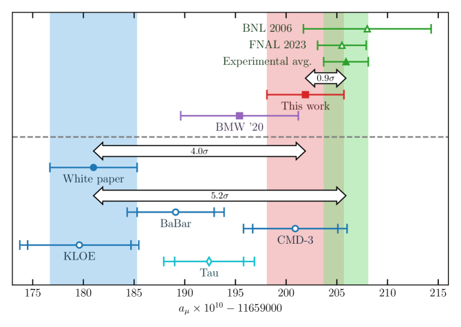
Figure 3: Comparison of standard-model predictions of the muon anomalous magnetic moment with its measured value. The panel above the dashed horizontal line shows a comparison of the world-average measurement of $a_{\mu}$ [116] denoted by a green band, with the standard-model prediction obtained here, denoted by the red band. The latter is obtained by adding the value of $a_{\mu}^{\text{LO-HVP}}$ computed in present work to the results for all of the other contributions summarised in Ref. [115]. The panel below the line shows the predictions for $a_{\mu}^{\text{LO-HVP}}$ obtained in the data-driven approach using the most precise measurements of the two-pion spectrum in electron-positron annihilation and $\tau$-decay experiments [118]. These correspond to BaBar [103, 104], KLOE [106, 107, 108, 109] and CMD-3 [105] for $e^{+}e^{-}$ annihilation and Tau for $\tau$ decays [119, 120]. The blue band shows the muon $g-2$ Theory Initiative combination of the data-driven results [115] (White paper), obtained prior to the publication of the CMD-3 measurement. That combination is currently being reassessed. The error bars are SEM.

Acknowledgements: The authors gratefully acknowledge the Gauss Centre for Supercomputing (GCS) e.V. [46], GENCI [47] (grant 502275) and EuroHPC Joint Undertaking (grant EXT-2023E02-063) for providing computer time on the GCS supercomputers SuperMUC-NG at Leibniz Supercomputing Centre in München, HAWK at the High Performance Computing Center in Stuttgart and JUWELS and JURECA at Forschungszentrum Jülich, as well as on the GENCI supercomputers Joliot-Curie/Irène Rome at TGCC, Jean-Zay V100 at IDRIS, Adastra at CINES and on the Leonardo supercomputer hosted at CINECA. This work received funding from the French National Research Agency under contract ANR-22-CE31-0011, from the Excellence Initiative of Aix-Marseille University – A*Midex, a French “Investissements d’Avenir” program under grants AMX-18-ACE-005, AMX-22-RE-AB-052, and from grants NW21-024-A and BMBF-05P21PXFCA. AB, ZF, DG and AK are supported by ERC-MUON-101054515. ZF is also partially supported by NW21-024-B and DOE-0000278885. AP is partly supported by UK STFC Grant ST/X000494/1 and by long-term Invitational Fellowship L23530 from the Japan Society for the Promotion of Science.

center Supplementary Information
High precision calculation of the hadronic vacuum polarisation contribution to the muon anomaly A. Boccaletti^1,2, Sz. Borsanyi¹, M. Davier³, Z. Fodor^{1,4,5,2,6,7,∗}, F. Frech¹, A. Gérardin⁸, D. Giusti^2,9, A.Yu. Kotov², L. Lellouch⁸, Th. Lippert², A. Lupo⁸, B. Malaescu¹⁰, S. Mutzel^8,11, A. Portelli^12,13, A. Risch¹, M. Sjö⁸, F. Stokes^2,14, K.K. Szabo^1,2, B.C. Toth¹, G. Wang⁸, Z. Zhang³

¹ Department of Physics, University of Wuppertal, D-42119 Wuppertal, Germany
² Jülich Supercomputing Centre, Forschungszentrum Jülich, D-52428 Jülich, Germany
³ IJCLab, Université Paris-Saclay et CNRS/IN2P3, Orsay, 91405, France
⁴ Physics Department, Pennsylvania State University, University Park, PA 16802, USA
⁵ Institute for Computational and Data Sciences, Pennsylvania State University, University Park, PA 16802, USA
⁶ Institute for Theoretical Physics, Eötvös University, H-1117 Budapest, Hungary
⁷ University of California, San Diego, 9500 Gilman Drive, La Jolla, CA 92093, USA
⁸ Aix Marseille Univ, Université de Toulon, CNRS, CPT, IPhU, Marseille, France
⁹ Fakultät für Physik, Universität Regensburg, 93040, Regensburg, Germany
¹⁰ LPNHE, Sorbonne Université, Université Paris Cité, CNRS/IN2P3, Paris, 75252, France
¹¹ Laboratoire de Physique de l’Ecole Normale Supérieure, Mines Paris - PSL, CNRS, Inria, PSL Research University, Paris, France
¹² School of Physics and Astronomy, University of Edinburgh, Edinburgh EH9 3JZ, United Kingdom
¹³ RIKEN Center for Computational Science, Kobe 650-0047, Japan
¹⁴ Special Research Centre for the Subatomic Structure of Matter, Department of Physics University of Adelaide, South Australia 5005, Australia

1 Configuration and measurements

1.1 Action and ensembles

We perform simulations using the 4stout lattice action, which is defined by the tree-level Symanzik gauge action [48] and a one-link staggered fermion action. Where the gauge link appears in the fermion action, we apply four steps of stout smearing [49] with a smearing parameter of $\rho=0.125$.

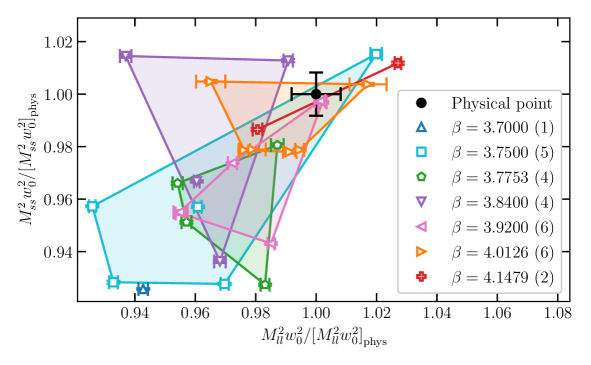
Figure 1: Landscape of our ensembles. The horizontal and vertical axes are the squared pseudo-scalar masses, $M_{ll}^{2}$ and $M_{ss}^{2}$, in units of the $w_{0}$-scale, both normalized with the respective physical value. Different colors denote different lattice spacings and the black point denotes the (isospin-symmetric) physical point. The uncertainties of this point are coming from our determination of the $M_{ll},M_{ss}$ and $w_{0}$ parameters in physical units.

$\beta$	$a$ [fm]	$L/a\times T/a$	tag	$am_{s}$	$m_{s}/m_{l}$	#confs
3.7000	0.1315	$48\times 64$	dir00	0.057291	27.899	904
3.7500	0.1191	$56\times 96$	dir00	0.049593	28.038	315
			dir01	0.049593	26.939	516
			dir02	0.051617	29.183	504
			dir03	0.051617	28.038	522
			dir05	0.055666	28.083	215
3.7753	0.1116	$56\times 84$	dir00	0.047615	27.843	510
			dir01	0.048567	28.400	505
			dir02	0.046186	26.469	507
			dir03	0.049520	27.852	385
3.8400	0.0952	$64\times 96$	dir00	0.043194	28.500	510
			dir02b	0.043194	30.205	436
			dir04	0.040750	28.007	1503
			dir05	0.039130	26.893	500
3.9200	0.0787	$80\times 128$	dir02	0.032440	27.679	506
			dir04	0.034240	27.502	512
			dir01b	0.032000	26.512	1001
			dir02b	0.032440	27.679	327
			dir03b	0.033286	27.738	1450
			dir04b	0.034240	27.502	500
4.0126	0.0640	$96\times 144$	phys1	0.026500	27.634	446
			phys2	0.026500	27.124	551
			phy1b	0.026500	27.634	2248
			phys2b	0.026500	27.124	1000
			phys3	0.027318	27.263	985
			phys4	0.027318	28.695	1750
4.1479	0.0483	$128\times 192$	phys1	0.019370	27.630	2792
			phys2	0.019951	27.104	2225

Table 1: List of the ensembles used in this work, with gauge coupling, lattice spacing, lattice size, ensemble tag, strange quark mass, mass ratio of strange and light quarks and number of configurations.

We use $2+1+1$ dynamical flavors with equal up and down quark masses $m_{u}=m_{d}=m_{l}$. The mass parameters for the light $m_{l}$ and the strange quark $m_{s}$ are chosen to scatter around the physical point. This can be seen in Figure 1, where we show the landscape of our ensembles in the plane of the light and strange quark masses. The charm mass parameter is set by the ratio $m_{c}/m_{s}=11.85$, which was taken from the charm meson analysis in [50]. This value is within one per-cent of the most recent lattice average from FLAG [51]. We use seven different values for the gauge coupling parameter $\beta$. The corresponding lattice spacings and the set of ensembles at each lattice spacing, together with the number of configurations are listed in Table 1. Most of the ensembles in this study were also used in our earlier work on the magnetic moment of the muon [52]. Since then we added a finer lattice spacing with $\beta=4.1479$ with two different ensembles, which bracket the physical point in both the light and the strange quark mass.

To set the scale and the physical point we use the Wilson-flow-based observable $w_{0}$ and the masses of connected pseudo-scalar mesons built from the different quark flavors. The physical values of these observables were computed in our earlier work [52], where we used the experimental values of the hadron masses $\pi^{0}$, $K^{+}$, $K^{0}$ and $\Omega^{-}$ as inputs. A more detailed discussion about our setting of the physical point is given in Section 3.

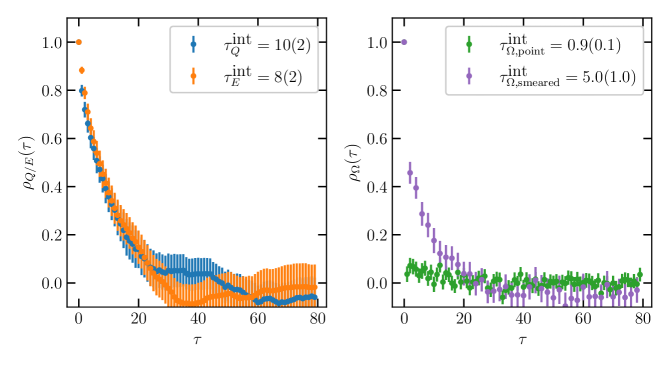
Figure 2: Left panel: normalized autocorrelation function of energy density $E$ and topological charge $Q$, both computed at a gradient-flow time of $w_{0}^{2}$ on one of the ensembles at $\beta=4.1479$. Right panel: normalized autocorrelation function of the $\Omega_{\mathrm{VI}}$ hadron correlator with point and smeared sources. The correlator is taken at $t=1.5~{}\mathrm{fm}$ time separation, which is located in the middle of the fitting window. The plots also include the integrated autocorrelation times for each observable.

The configurations are generated with a Rational Hybrid Monte Carlo algorithm [53] including force gradient [54], multiple timescales [55] and Hasenbusch preconditioning [56]. The configurations are separated by 10 unit length trajectories. In Figure 2 we show normalized autocorrelation functions, denoted here by $\rho(\tau)$, for the topological charge, smeared energy density and Omega propagator. The charge is computed using the standard clover discretisation of the topological charge density at a gradient-flow time of $w_{0}^{2}$, which corresponds to a smearing radius of about $0.5\mathrm{fm}$. The same flow-time is used for the smeared energy density. The autocorrelation function and its error are computed using the pyerrors package [57]. The integrated autocorrelation time of the topological charge and the smeared energy density in this ensemble is $10(2)$, given in units of configurations. The autocorrelation time of the $\Omega_{\mathrm{VI}}$-propagator is somewhat smaller, see Figure 2. The definition of $\Omega_{\mathrm{VI}}$ is given in Section 2.

We use jackknife resampling to calculate the statistical errors. To suppress the auto-correlation between data from subsequent configurations we introduce a blocking procedure. It is very convenient to use an equal number of blocks for all ensembles. In this work we use 48 blocks. With this choice we have typically 10 configurations or more in a block, which is larger than the autocorrelation time of any of the quantities we consider even on our finest ensembles, as shown in Figure 2. For the blocks we apply the delete-one principle, resulting in 48 jackknife samples plus the full sample.

1.2 Taste violation

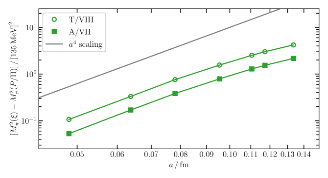
Figure 3: Taste violation as a function of lattice spacing, for axial-vector $A$ and tensor $T$ tastes. The Roman-number labeling of the tastes is taken from [58], e.g. the pseudo-scalar taste $P$ corresponds to II.

An important aspect of these computations is the lattice artefact related to the taste symmetry violation of staggered fermions. This makes pseudo-scalar mesons heavier than in the continuum, depending on their taste quantum number. In particular the masses of pions and eta mesons built from light quark flavors are given as:

$$M^{2}_{\pi}(\xi)=M^{2}_{ll}+\Delta_{KS}(\xi)\quad\text{and}\quad M^{2}_{\eta}(\xi)=M^{2}_{ll}+\Delta_{KS}(\xi)+\tfrac{1}{2}\delta_{KS}(\xi)$$ (1)

where $M^{2}_{ll}$ is the squared mass of the usual pseudo-Goldstone pion. The pions have only connected contractions, whereas the etas also contain disconnected contributions. The $\xi$ stands for one of the sixteen meson tastes of the taste $SU(4)$ group. In practical lattice simulations these group into multiplets of the $SO(4)$ group to a very good approximation, so the meson tastes are conventionally labeled by $P,A,T,V,I$. The $P$ taste corresponds to the pseudo-Goldstone pion, for which $\Delta_{KS}(P)$ and $\delta_{KS}(P)$ are zero.

We compute the taste-symmetry breaking terms $\Delta_{KS}(\xi)$ by comparing the masses of different meson tastes on our ensembles. For this purpose we use an average “flavor-symmetric” valence quark mass of $\tfrac{1}{3}(2m_{l}+m_{s})$. In Figure 3 we show this comparison for the $A$ and $T$ tastes as a function of the lattice spacing. We observe a decrease with approximately the fourth power of the lattice spacing towards our finer lattices. This is much faster than the $\alpha_{s}a^{2}$ expected from naive scaling, where $\alpha_{s}$ is the strong coupling constant at the lattice cutoff scale. The falloff is actually consistent with an $\alpha_{s}^{n}a^{2}$ type behavior with $n=3$. We will use $\Delta_{KS}(A)$, when parameterizing lattice artefacts in our continuum extrapolation procedure, described in Section 4.

The taste-symmetry breaking terms $\delta_{KS}(\xi)$ are related to the eta mesons. $\delta_{KS}(T)=0$ in the $SO(4)$ approximation, $\delta_{KS}(I)$ arises from the chiral anomaly, and $\delta_{KS}(A)$ and $\delta_{KS}(V)$ are called hairpin parameters. These have never been measured directly, since the disconnected contributions are computationally demanding. It is usually assumed that these artefacts decrease with the same rate as $\Delta_{KS}(\xi)$, see e.g. in [59].

2 Omega baryon mass measurements

To extract the mass of the positive-parity, ground-state $\Omega$ baryon, we use a similar strategy as in our previous work [52]. In particular we consider three different operators [60, 58, 61]:

$$\begin{aligned} \Omega_{\rm{VI}}(t)&=\sum_{x_{k}even}\epsilon_{abc}\left[S_{1}\chi_{a}S_{12}\chi_{b}S_{13}\chi_{c}-S_{2}\chi_{a}S_{21}\chi_{b}S_{23}\chi_{c}+S_{3}\chi_{a}S_{31}\chi_{b}S_{32}\chi_{c}\right](x)\\ \Omega_{\rm{XI}}(t)&=\sum_{x_{k}even}\epsilon_{abc}\left[S_{1}\chi_{a}S_{2}\chi_{b}S_{3}\chi_{c}\right](x)\\ \Omega_{\rm{Ba}}(t)&=[2\delta_{\alpha 1}\delta_{\beta 2}\delta_{\gamma 3}-\delta_{\alpha 3}\delta_{\beta 1}\delta_{\gamma 2}-\delta_{\alpha 2}\delta_{\beta 3}\delta_{\gamma 1}+(\cdots\beta\leftrightarrow\gamma\cdots)]\\ &\sum_{x_{k}even}\epsilon_{abc}\left[S_{1}\chi_{a\alpha}S_{12}\chi_{b\beta}S_{13}\chi_{c\gamma}-S_{2}\chi_{a\alpha}S_{21}\chi_{b\beta}S_{23}\chi_{c\gamma}+S_{3}\chi_{a\alpha}S_{31}\chi_{b\beta}S_{32}\chi_{c\gamma}\right](x)\end{aligned}$$ (2)

Here, $\chi_{a}(x)$ is the strange-quark field with color index $a$ and $\chi_{a\alpha}(x)$ with $\alpha=1,2,3$ the additional “flavor” index introduced by Bailey [61]. The operator $S_{\mu}$ performs a symmetric, gauge-covariant shift in direction $\mu$, while $S_{\mu\nu}\equiv S_{\mu}S_{\nu}$. $\Omega_{\rm{VI}}$ and $\Omega_{\rm{XI}}$ couple to two different tastes of the $\Omega$ baryon and $\Omega_{\rm{Ba}}$ only couples to a single taste. In the continuum limit the mass of these states becomes degenerate. In our analyses we include all three in order to assign a systematic to the choice of the operator.

Beside point sources we also use smeared ones to construct the propagator. Smearing changes the excited state contamination and including smeared propagators in the analysis makes a more reliable extraction of the ground state possible. These propagators are constructed by applying spatial Wuppertal smearing [62] on a source $\psi$ vector

$$[\hat{W}\psi]_{x}=(1-\sigma)\psi_{x}+\frac{\sigma}{6}\sum_{\mu=1,2,3}\left(U_{\mu,x}^{\mathrm{3d}}U_{\mu,x+\mu}^{\mathrm{3d}}\psi_{x+2\mu}+U_{\mu,x-\mu}^{\mathrm{3d},\dagger}U_{\mu,x-2\mu}^{\mathrm{3d},\dagger}\psi_{x-2\mu}\right)$$ (3)

with smearing parameters $\sigma=0.5$. The spatial derivatives involve two hops in order to preserve the staggered symmetries of the operators. They also include a smeared-gauge field $U^{\mathrm{3d}}$ obtained by applying $N_{\mathrm{3d}}$ spatial stout smearing steps with smearing parameters $0.125$. The smeared source is then obtained by applying the Wuppertal-smearing procedure $N_{\mathrm{Wptl}}$ times on a point source. The number of smearing steps, see Table 2, depends on the $\beta$ in such a way to keep the effective smearing radius of the procedure approximately constant in physical units.

$\beta$	$N_{\rm{Wptl}}$	$N_{\rm{3d}}$	$t_{p}$	$t_{a}$	$t_{b}$	range #1	range #2	# pt, sm sources
3.7000	24	32	1	4	7	7$\dots$15	8$\dots$15	28928, 229376
3.7500	30	40	1	4	7	8$\dots$18	9$\dots$18	66208, 530176
3.7553	34	46	1	4	7	9$\dots$19	10$\dots$19	61024, 488192
3.8400	46	62	2	4	9	10$\dots$20	11$\dots$20	125440, 2807552
3.9200	67	90	2	6	9	12$\dots$25	13$\dots$25	137472, 3038720
4.0126	101	135	3	6	9	15$\dots$30	16$\dots$30	223360, 4235520
4.1479	178	238	5	6	11	19$\dots$40	21$\dots$40	160544, 2068736

Table 2: Parameters of our procedure to obtain $\Omega$ mass: number of Wuppertal and stout smearing steps; the parameters $t_{p}$, $t_{a}$ and $t_{b}$ of the GEVP procedure and two different fit ranges, given by start and end points $t_{\mathrm{min}}$ and $t_{\mathrm{max}}$. For the definitions see the text. In the last column the total number of measurements with point and smeared sources are given.

To enhance the signal, we calculate the $\Omega$ propagators using $256$ or $512$ smeared and $32$ point source fields per gauge configuration; the total number of measurements for each $\beta$ are given in the last column of Table 2. For each source field we select a random time slice, which, in turn, is populated with eight independent $\mathbb{Z}_{3}$ random point sources at $(0,0,0)$, $(L/2,0,0)$, $\cdots$ and $(L/2,L/2,L/2)$.

We use a mass extraction procedure proposed in Ref. [63], which is based on the Generalized Eigenvalue Problem (GEVP). We first apply a folding transformation to the original hadron propagator $H_{t}$:

$$H_{t}\rightarrow\left\{\begin{matrix}[l]\;\frac{1}{2}\left[H_{t}+(-1)^{t+1}H_{T-t}\right]&0<t<\frac{T}{2}\\ \;H_{t}&t=0\;{\rm{or}}\;t=\frac{T}{2}\end{matrix}\right.\ ,$$ (4)

where the staggered phase factor $(-1)^{t+1}$ ensures the parity is consistent between the forward and backward-propagating states in the folding. Then for each time slice $t$ we construct the following $6\times 6$ matrix:

$$\mathbf{H}(t)=\left(\begin{array}[]{cc|cccc}H_{t+2t_{p}+0}^{pp}&H_{t+2t_{p}+1}^{pp}&H_{t+t_{p}+0}^{ps}&H_{t+t_{p}+1}^{ps}&H_{t+t_{p}+2}^{ps}&H_{t+t_{p}+3}^{ps}\\ H_{t+2t_{p}+1}^{pp}&H_{t+2t_{p}+2}^{pp}&H_{t+t_{p}+1}^{ps}&H_{t+t_{p}+2}^{ps}&H_{t+t_{p}+3}^{ps}&H_{t+t_{p}+4}^{ps}\\ \hline\cr H_{t+t_{p}+0}^{sp}&H_{t+t_{p}+1}^{sp}&H_{t+0}^{ss}&H_{t+1}^{ss}&H_{t+2}^{ss}&H_{t+3}^{ss}\\ H_{t+t_{p}+1}^{sp}&H_{t+t_{p}+2}^{sp}&H_{t+1}^{ss}&H_{t+2}^{ss}&H_{t+3}^{ss}&H_{t+4}^{ss}\\ H_{t+t_{p}+2}^{sp}&H_{t+t_{p}+3}^{sp}&H_{t+2}^{ss}&H_{t+3}^{ss}&H_{t+4}^{ss}&H_{t+5}^{ss}\\ H_{t+t_{p}+3}^{sp}&H_{t+t_{p}+4}^{sp}&H_{t+3}^{ss}&H_{t+4}^{ss}&H_{t+5}^{ss}&H_{t+6}^{ss}\end{array}\right)\ ,$$ (5)

where $\mathrm{type}$ in $H_{t}^{\mathrm{type}}$ denotes the different source-sink combinations, such as point-point, smear-point, point-smear and smear-smear, labeled with $pp$, $sp$, $ps$ and $ss$. We introduce an additional time shift $t_{p}$ in case of the point source operator to suppress its excited states. The time shifts between different rows and columns are needed to fully resolve the negative parity states, which have a negative amplitude.

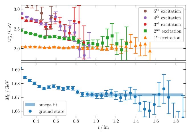
Figure 4: $\Omega$ baryon effective masses extracted from the GEVP for five excited states (upper panel) and for the ground state (lower panel) on an ensemble at $\beta=4.1479$. In the lower panel the blue band is obtained from a single exponential fit to the ground state propagator. In the upper panel the gray horizontal line corresponds to the mass of the recent observation of an excited $\Omega$ baryon from the Belle experiment [64]. To convert the numbers into physical units we used $a=0.0483~{}\mathrm{fm}$ lattice spacing here.

For a given $t_{a}$ and $t_{b}$, let $\lambda(t_{a},t_{b})$ be an eigenvalue and $v(t_{a},t_{b})$ an eigenvector of the following GEVP:

$$\mathbf{H}(t_{a})v(t_{a},t_{b})=\lambda(t_{a},t_{b})\mathbf{H}(t_{b})v(t_{a},t_{b})\ .$$ (6)

The ground state corresponds to the largest eigenvalue. The propagator corresponding to the eigenvector $v$ is given by vector-matrix-vector product:

$$P(t;t_{a},t_{b})=v^{\dagger}(t_{a},t_{b})\mathbf{H}(t)v(t_{a},t_{b})\ .$$ (7)

This correlation function can be fitted to an exponential function $A\exp(-Mt)$ with amplitude $A$ and mass $M$. Note, that backward propagating states have negligible contribution for the time-slices, that we work with. From $P(t)$ one can also construct an effective mass in the standard way. The tuneable parameters of the procedure are $t_{a}$ and $t_{b}$ for specifying the GEVP, as well as the fit range $[t_{\mathrm{min}},t_{\mathrm{max}}]$ for the exponential fitting.

In Figure 4 we show the effective masses obtained with the GEVP procedure for an ensemble at $\beta=4.1479$. As shown in the lower panel, the ground state is well resolved with a per-mill level of precision. The upper panel shows the excited states. The phenomenological interpretation of these is non-trivial, since they are hadron resonances decaying into scattering states. As an illustration we show the excited, negative-parity $\Omega$ baryon from the Belle experiment [64] with a mass of $2012.4(7)(6)~{}\mathrm{MeV}$.

We perform the exponential fit with taking into account the correlations between different timeslices in the $P(t)$ propagator. For that we construct the covariance matrix with $200$ jackknife samples, instead of our usual choice of $48$ samples, in order to have a more stable inverse matrix. Even the smaller block-size should not be problematic with the $\Omega$, its autocorrelation time is given in Section 1. When inverting the covariance matrix we apply a singular value decomposition and regulate the smallest eigenvalues of the correlation matrix as described in Appendix A.1 of Ref. [65]. In an uncorrelated fit or in a correlated fit with regulated eigenvalues the statistical interpretation of the fit quality becomes questionable. Recently an improved estimator for the fit quality was given in [66], which we call $Q$-value here. It can be employed both in the uncorrelated and correlated cases.

Figure 5: Left panel: cumulative distribution function (CDF) of $Q$-values [66] over all of our ensembles, where we show results for our two preferred fit-ranges and with the $\Omega_{\mathrm{VI}}$ operator. The first fit-range, shown with blue, is $[0.9\,\mathrm{fm},2.0\,\mathrm{fm}]$, whose Kolmogorov-Smirnov significance level is $P=0.09$, ie. the probability we get the observed CDF or anything worse is 9%, assuming a uniform distribution. We also use a second fit-range $[1.0\,\mathrm{fm},2.0\,\mathrm{fm}]$, shown with orange, with $P=0.36$. The green line represents the CDF of a hypothetical uniform distribution. Right panel: we show the Kolmogorov-Smirnov significance level for several different fit-ranges, $[t_{\mathrm{min}},t_{\mathrm{max}}]$, the brighter/darker colors stand for better/worse significance. Our final choices for the above two fit-ranges are shown by the red crosses.

The time range in the exponential fit is going to be chosen by the $Q$-value of the fit. For each operator in Equation (2) we compute the $Q$-values on all of our ensembles for several different fit ranges $[t_{\mathrm{min}},t_{\mathrm{max}}]$. In the left panel of Figure 5 we show the cumulative distribution function of the $Q$-values over all of our ensembles for some selected fit-ranges and for the $\Omega_{\mathrm{VI}}$ operator. For a given fit range the $Q$-values will follow a uniform distribution, if the ground state correlator $P(t)$ can be described by a single exponential $A\exp(-Mt)$. To decide, if the observed CDF is uniform, we use a one-sided Kolmogorov-Smirnov test with the uniform distribution of the $Q$-values as null-hypothesis. We vary the fit-ranges and compute the Kolmogorov-Smirnov significance. These are shown in a heat-map format in the right panel of Figure 5. We choose to work with the fit-range $[0.9\,\rm{fm},2.0\,\rm{fm}]$. To estimate the systematic error related to the fit-range we also use one with a later start, $[1.0\,\rm{fm},2.0\,\rm{fm}]$. Both ranges are plotted on the heatmap figure, with red crosses.

The extracted ground state energies for all of our ensembles are given in Figure 6. We reach better than $0.1$% precision on our finest lattice. We see an increase of the precision towards finer lattice spacings, this can be partly explained by the increase in the number of measurements with $\beta$. In order to see the robustness of our procedure, we also performed fits without taking into account correlations between the timeslices. The results of these are also shown in Figure 6 and they are well consistent with the correlated ones.

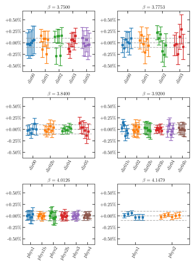
Figure 6: Results for the ground state $\Omega$ baryon mass with fit range $[0.9\,\mathrm{fm},2.0\,\mathrm{fm}]$ on different ensembles. Each ensemble has six data points with the same color, which correspond to correlated fits to the $\Omega_{\rm{VI}}$, $\Omega_{\rm{XI}}$ and $\Omega_{\rm{Ba}}$ propagators followed by the same propagators in uncorrelated fits. The plot shows the relative deviation from the ensemble average, ie. the average over the six points with the same color. The upper and lower dashed lines show $\pm 0.1$% error bands.

3 Physical point and isospin decomposition

In our computations we use the masses of $\pi^{0}$, $K^{+}$ and $K^{0}$ pseudoscalar mesons and the mass of the $\Omega^{-}$ baryon to set the physical point in the full theory, i.e. in QCD plus QED. In addition we also need a way of separating pure QCD effects from electromagnetic ones. The separation implies the definition of the physical point in pure QCD. Here this is achieved by choosing a set of observables, whose physical values we take the same in QCD as in the full-theory. The definition of course is not unique and will depend on the choice of observables. As a consequence pure QCD results have a scheme ambiguity, which one has to keep in mind, when doing comparisons.

To choose the set of variables, we follow our approach from our 2020 work [52]: we take the Wilson-flow-based $w_{0}$ scale and the fully connected up, down and strange meson masses $M_{uu}$, $M_{dd}$, and $M_{ss}$. These masses are computed by taking into account only the quark-connected contributions to their two-point functions as in Ref. [67], and can be defined rigorously in a partially-quenched theory. These mesons are neutral and have no magnetic moment, and are thus only weakly affected by electromagnetism. The same holds for the $w_{0}$ scale, therefore our observable set is a reasonable choice for the matching. We will use $\hat{M}$ to denote the average $\hat{M}^{2}\equiv\tfrac{1}{2}\left(M^{2}_{uu}+M^{2}_{dd}\right)$. Also we will use $\Delta M^{2}$ as the difference $\Delta M^{2}\equiv M^{2}_{dd}-M^{2}_{uu}$, which is a measure of the strong isospin breaking. Our set of observables cannot be measured experimentally, but they have a well-defined continuum limit, so a physical value can be associated with each of them. These values can be computed in the full theory, where the masses of $\pi^{0}$, $K^{+}$, $K^{0}$ and $\Omega^{-}$ are set to their physical values.

A matching scheme can be used to split an observable $O$ into isospin-symmetric and isospin-breaking contributions. This is accomplished by studying the functional dependence of $O$ on the scheme-defining observables from above:

$$O(\hat{M}w_{0},M_{ss}w_{0},\Delta M^{2}w_{0}^{2},e)\ ,$$ (8)

where $e$ is the electromagnetic coupling. The isospin-symmetric component of $O$ is given by

$$[O]_{\mathrm{iso}}=O\left([\hat{M}w_{0}]_{\mathrm{phys}},[M_{ss}w_{0}]_{\mathrm{phys}},0,0\right)\ ,$$ (9)

where “$\mathrm{phys}$” denotes the physical value in the full theory. The value of $[O]_{\mathrm{iso}}$ can be determined from isospin-symmetric measurements alone, where the average pion mass $\hat{M}$ equals $M_{ll}$, the mass of the meson constructed from light sea quarks. The strong-isospin-breaking contribution is given by

$$[O]_{\mathrm{sib}}=O\left([\hat{M}w_{0}]_{\mathrm{phys}},[M_{ss}w_{0}]_{\mathrm{phys}},[\Delta M^{2}w_{0}^{2}]_{\mathrm{phys}},0\right)-[O]_{\mathrm{iso}}\ .$$ (10)

If we are interested only in the leading-order of this breaking, like in this work where we neglect higher order effects, we can use the following derivative:

$$[O]_{\mathrm{sib}}=[\Delta M^{2}w_{0}^{2}]_{\mathrm{phys}}\times\frac{\partial O}{\partial(\Delta M^{2}w_{0}^{2})}\left([\hat{M}w_{0}]_{\mathrm{phys}},[M_{ss}w_{0}]_{\mathrm{phys}},0,0\right)\ .$$ (11)

The sum of the isospin-symmetric and strong-isospin-breaking contributions gives the total pure QCD value: $[O]_{\mathrm{qcd}}=[O]_{\mathrm{iso}}+[O]_{\mathrm{sib}}$. The electromagnetic part is given by the difference

$$[O]_{\mathrm{qed}}=O\left([\hat{M}w_{0}]_{\mathrm{phys}},[M_{ss}w_{0}]_{\mathrm{phys}},[\Delta M^{2}w_{0}^{2}]_{\mathrm{phys}},e\right)-[O]_{\mathrm{qcd}}\ .$$ (12)

Finally, the total physical value is the sum of all components: $[O]_{\mathrm{phys}}=[O]_{\mathrm{iso}}+[O]_{\mathrm{sib}}+[O]_{\mathrm{qed}}$. In this work we compute the isospin symmetric part of the hadronic vacuum polarization, the strong-isospin-breaking and electromagnetic parts will be taken from our 2020 publication.

3.1 Physical values of $M_{uu}$, $M_{dd}$, $M_{ss}$ and $w_{0}$

Now let us turn to physical values of the scheme-defining observables. The physical value of $\hat{M}$ can be obtained from leading-order partially-quenched chiral perturbation theory coupled to photons [68], according to which $\hat{M}$ equals the neutral pion mass, i.e.

$$[\hat{M}]_{\mathrm{phys}}=134.9768(5)~{}\mathrm{MeV}.$$ (13)

Here the equality is valid up to next-to-leading order effects in the isospin-breaking, which we neglect here. For physical values of the remaining meson masses we use the analysis from 2020, and we give them for completeness here:

_phys $$=13170(320)(270)[420]~{}\mathrm{MeV}^{2},$$ (14)

$$[M_{ss}]_{\mathrm{phys}} =689.89(28)(40)[49]~{}\mathrm{MeV},$$

where the first error is statistical, the second is systematic and the third is the total.

The physical value of the gradient-flow scale $w_{0}$ was already computed in our 2020 work. Here we compute it with an increased precision by adding the $0.048$ fm lattice spacing into the analysis and obtain:

_phys $$=0.17245(22)(46)[51]~{}\mathrm{fm}\ ,$$ (15)

again with statistical, systematic and total errors. The analysis we perform is called “Type-I” fit in our 2020 work, and it uses the $M_{\Omega}$, $M_{K}$ and $M_{\pi}$ masses as input. The current analysis consists of $8640$ fits, differing in the fit ranges of the pseudoscalars and the omega baryon, the cuts in the lattice spacing and the functional form of the fit function. We also vary the expansion variable between a naive $a^{2}$ and a $\Delta_{KS}(a)$ type dependence in the lattice spacing. As opposed to our earlier publication in 2020, where we used only quadratic polynomials of the expansion variable, this time we also include cubic ones. The analysis is performed by using the isospin-symmetric data-sets only, the isospin-breaking contributions were taken from our 2020 work. Sample continuum extrapolations, probability distribution function and error budget are shown in Table 3.

Median	172.35 am
Total error	0.51 am	0.30 %
Statistical error	0.22 am	0.13 %
Systematic error	0.46 am	0.27 %
Pseudoscalar fit range	0.01 am	$<$ 0.01 %
Omega baryon fit range	0.24 am	0.14 %
Physical value of $M_{\Omega}$	0.06 am	0.03 %
Lattice spacing cuts	0.09 am	0.05 %
Order of fit polynomials	0.17 am	0.10 %
Continuum parameter ($\Delta_{KS}$ or $a^{2}$)	0.30 am	0.17 %

Table 3: Gradient flow scale $w_{0}$. Continuum extrapolations as function of $a^{2}$ and as function of $\Delta_{KS}$ are shown in the first row. In the figure in the second row the probability distribution function (PDF) including both statistical and systematic variations is shown with red color. The median is given by the blue horizontal line, the 1-sigma/2-sigma error band defined from the 16%/2% and 84%/98% percentiles is shown with green/yellow color. The table in the third row shows the total, statistical and systematic errors, and also displays an error budget.

The errors in the physical input quantities and also their correlations are incorporated in our analyses by a stochastic sampling of their respective distributions. More details on this procedure are given in Section 4.

3.2 Kaon mass decomposition in different schemes

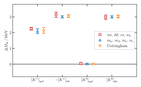
Figure 7: Decomposition of the neutral and charged kaon masses in three different isospin schemes. Red squares stand for our scheme from [52] based on the observables $\{M_{uu},M_{dd},M_{ss},w_{0}\}$, blue triangles for the GRS scheme based on quark masses and strong coupling constant taken from [69] and orange circles for a Cottingham-formula based decomposition given in [70].

The isospin-symmetric point depends on the observables that define it, an effect commonly referred to as scheme dependence. A similar scheme to ours was put forward already in Ref. [71], though the physical values of the defining observables were not computed there. A scheme based on the Lagrangian parameters of the theory, which keeps normalized quark masses and strong coupling constant while turning on the electromagnetic interaction, was proposed by Gasser, Rusetsky and Scimemi [72]. This scheme is called the GRS scheme in the literature and was implemented on the lattice in Ref. [73, 69]. Finally, in phenomenological computations one often uses a scheme based on the Cottingham formula [74], which gives the electromagnetic contribution to the hadron masses, for a concrete application see Ref. [70].

To compare our scheme with others we decompose the neutral and charged kaon masses into isospin components. For this purpose we perform an analysis that is described as a Type-II fit in our 2020 work. We consider the dependence of the kaon masses on our scheme defining observables according to Equation (8), and use their physical values as inputs. The procedure also takes into account electromagnetic effects. It includes about ten-thousand fits to estimate systematics related to e.g. continuum extrapolation and choice of the mass fit range. The decomposition we obtain is

$$[M_{K^{0/+}}]_{\mathrm{iso}}=494.55(31)~{}\mathrm{MeV}\begin{aligned} \quad\quad[M_{K^{0}}]_{\mathrm{sib}}=&+2.98(14)~{}\mathrm{MeV}\quad\quad&[M_{K^{0}}]_{\mathrm{qed}}&=0.05(7)~{}\mathrm{MeV}\\ \quad\quad[M_{K^{+}}]_{\mathrm{sib}}=&-3.13(17)~{}\mathrm{MeV}\quad\quad&[M_{K^{+}}]_{\mathrm{qed}}&=2.25(8)~{}\mathrm{MeV}\\ \end{aligned}$$ (16)

where the uncertainties given are the statistical and systematic errors added in quadrature. Figure 7 shows a comparison with the same decomposition in other schemes, whose values were taken from Refs. [73, 70]. We find a good agreement with the scheme based on quark masses (GRS) and with the one based on the Cottingham-formula. In addition we note here, that our isospin-symmetric kaon mass agrees nicely with the GRS scheme value $[M_{K}]_{\mathrm{iso}{},\mathrm{GRS}}=494.6(1)$, computed in [69]. An agreement on the kaon decomposition is a strong indication for the equivalence of two schemes. Indeed, since the pion mass splitting only receives electromagnetic isospin-breaking effects at the first-order, most of the scheme dependence is concentrated in the decomposition of the kaon mass splitting.

4 Analysis procedure

4.1 Extrapolation functions

In order to obtain the physical isospin-symmetric values of the different windows in the hadron vacuum polarization we perform global fits to the lattice spacing and quark mass dependence of these observables.

Naïvely, we expect the leading discretisation errors to scale like $a^{2}$. In general, however, this is modified to $\alpha_{s}^{n}a^{2}$ by anomalous dimensions of operators in the Symanzik effective theory [75], where $\alpha_{s}$ is the strong coupling at the scale of the lattice spacing. The correct value of $n$ is not known a priori for our lattice action and observables. To account for this uncertainty, we perform fits with two different values of $n$. Firstly, we include a conventional polynomial in $a^{2}/w_{0}^{2}$, corresponding to $n=0$, which we label $A(a^{2})$. For a second value of $n$, we note that towards our finest lattice spacings the taste-symmetry violation decreases approximately as $\alpha_{s}^{n}a^{2}$ with $n=3$, as was discussed in Section 1. Therefore we will use a second type of polynomial $A^{\prime}(\Delta_{KS})$, where the variable $\Delta_{KS}$ measures the taste violation. For this we take a dimensionless combination of the axial-vector taste splitting and the $w_{0}$-scale, i.e. $\Delta_{KS}w_{0}^{2}\equiv\Delta_{KS}(A)w_{0}^{2}$. We will show the difference between $A(a^{2})$ and $A^{\prime}(\Delta_{KS})$ fits for several observables in Section 5. As we will see there, the $A^{\prime}(\Delta_{KS})$ continuum extrapolations have in general less curvature and a shorter extrapolation distance.

For the quark mass dependence, the variables

$$X_{l}=\hat{M}^{2}w_{0}^{2}-{\big{[}\hat{M}^{2}w_{0}^{2}\big{]}}_{\mathrm{phys}}\quad\text{and}\quad X_{s}=M_{ss}^{2}w_{0}^{2}-{\big{[}M_{ss}^{2}w_{0}^{2}\big{]}}_{\mathrm{phys}}$$ (17)

describe the deviation from the physical light and strange quark mass respectively. Here “phys” denotes the physical values given in Equations (13), (14) and (15). In case of isospin-symmetric fits $\hat{M}$ is given by $M_{ll}$. In our global fit we consider terms linear in these variables. No higher orders are needed, since we work close to the physical point. We allow these terms to depend on the lattice spacing, so their coefficients become polynomials $B(a^{2})$ and $C(a^{2})$.

Putting all this together, the global fit function is

$$Y=A(a^{2})+A^{\prime}(\Delta_{KS})+B(a^{2})X_{l}+C(a^{2})X_{s}\ ,$$ (18)

where $Y$ is one of our dimensionless target observables. We consider different polynomial orders for $A$, $A^{\prime}$, $B$, and $C$, as well as omitting between zero and four of the coarsest lattice spacings (out of a total of seven) from the fits. For $A$ and $A^{\prime}$, we consider two scenarios: one where we parameterize the continuum limit in terms of $a^{2}$, by setting $A^{\prime}$ to zero, and letting $A$ be linear, quadratic or cubic in $a^{2}$; and one where we instead use $\Delta_{KS}$, by setting $A$ to zero and letting $A^{\prime}$ be linear, quadratic or cubic in $\Delta_{KS}$. For $B$ and $C$, we consider both constant and linear polynomials in $a^{2}$. For each combination of polynomial orders, we consider the lattice spacing cuts that leave at least one more lattice spacing than the total number of coefficients contained in $A$ or $A^{\prime}$, as well as at least two more lattice spacings than the maximum number of coefficients contained in $B$ or $C$.

When presenting results for the observables, we will show continuum extrapolation plots: data as a function of the $a^{2}$ or $\Delta_{KS}$ for a representative subset of the fits. On the plots the data-points are obtained by shifting the observables on the ensembles to the physical values of the light and strange masses using the $B$ and $C$ coefficients from the fit. The fit curves correspond to the fit functions with only the $A$ or $A^{\prime}$ terms kept.

4.2 Distribution of observables

For a given observable, fit function, lattice spacing cut ans some other systematics we assign a weight using the Akaike Information Criterion (AIC) in a modified version as derived in Ref. [52]:

$$w=\exp\left[-\frac{1}{2}\left(\chi^{2}+2n_{\mathrm{par}}-n_{\mathrm{data}}\right)\right]\ ,$$ (19)

computed from the $\chi^{2}$ of the fit, the number of parameters $n_{\mathrm{par}}$, and the number of data points included in the fit $n_{\mathrm{data}}$. The first two terms in the exponent correspond to the standard AIC, and the last term is introduced to weight fits with a different number of ensembles, due to our cuts in the lattice spacing. From these weighted fits we build a probability distribution from which central value, statistical and systematic errors for the observable $Y$ are constructed. The technique is described in detail in [52], we briefly summarize it below.

In order to estimate the statistical and systematic errors, the fit procedure is carried out on each jackknife sample with many different choices of the systematic ingredients. There are two different types of systematics: one where the different possibilities enter with equal weight (flat-weighted) and another where they enter with the AIC weight of their corresponding fit qualities (AIC-weighted). We label collectively the flat-weighted systematics with the indices $i,j$ and the AIC-weighted with the indices $a,b$. For each analysis, given by a pair of indices $(i,a)$, we have an average value $y_{ia}$, a jackknife error $\sigma_{ia}$ and an AIC weight $w_{ia}$ from Equation (19). From these inputs we construct a probability distribution function (PDF) for the observable $Y$

$$\mathrm{PDF}(Y)=\sum_{i,a}\frac{w_{ia}\cdot\mathcal{N}(y_{ia},\sigma_{ia};Y)}{\sum_{b}w_{ib}\cdot\sum_{j}1}\ ,$$ (20)

which includes both statistical and systematic variations. The statistical variations are assumed to follow a normal distribution, i.e. $\mathcal{N}(y,\sigma;Y)$ is a normal PDF with mean $y$ and standard deviation $\sigma$.

The central value of $Y$ is defined by the median of the constructed PDF. The lower and upper total errors are defined by the standard one-sigma quantiles of the corresponding cumulative distribution function (CDF), at approximately 16 and 84. A further estimate of the lower and upper errors comes from halving the intervals obtained from the standard two-sigma quantiles at approximately 2 and 98. Any difference between the two estimates is related to deviations of our distribution away from a normal distribution. To be conservative, for each quantity we consider here, we take the larger of these two error estimates to be our final error. The figures attached to this section show the PDF, the median and corresponding error bands. This procedure gives the total uncertainty of $Y$. It is also possible to decompose the total error into statistical and systematic components, and the latter into each individual systematic ingredient [52].

In Ref. [76] the same PDF as in Equation (20) is used, however error estimates are constructed using variances of this distribution instead from quantiles. Also the AIC-criterion of [76] differs from ours in Equation (19) in the way the lattice spacing cuts are implemented. For the error budgets given in the following tables we use the variance approach of [76] instead of our original proposal, since it gives very similar results for much less computational cost.

4.3 Combining distributions with random sampling

We will also need a technique to perform a stochastic sampling of the previously described PDF. This comes useful when combining several of such PDFs, each with tens of thousands of analyses, where taking into account all possible combinations would be unfeasible. We perform an importance-weighted stochastic sampling of the systematic ingredients. Let us consider two observables, $Y$ and $Z$, which share some systematic ingredients and their remaining ones are treated as independent. Then a random sample is constructed in the following way:

1. We make a random selection for the systematic ingredients shared by $Y$ and $Z$. (In our cases the shared ingredients are always flat-weighted, so we have a uniform distribution in this step.)

2. We make a random selection for the remaining independent ingredients with a probability given by

   $$P(i,a)=\frac{w_{ia}}{\sum_{b}w_{ib}\sum_{j}1}\ ,$$ (21)

   where in the sums the shared ingredients are fixed to the values selected in step 1. This is conveniently accomplished by choosing a uniform random number $r$ in the $[0,1]$ interval and picking the analysis where the CDF built from the $P(i,a)$ values first reaches the number $r$. This step has to be done for $Y$ and $Z$ independently.

3. We build the combination observable from $Y$ and $Z$ using the shared and unshared ingredients from steps 1. and 2.

To properly account for statistical correlations, we preserve the jackknife samples during the whole construction. Repeating these steps $N_{R}$ times, we obtain the desired distribution for the combination observable, which has a single systematic ingredient labeled by the sample index, and each of them comes with a flat weight of $1/N_{R}$. The statistical, systematic and total errors of the combination can then be obtained by our usual procedure as described above. A similar sampling technique was recently proposed in Ref. [77].

In order to obtain the physical value of an observable $Y$ we need the physical values of $w_{0}$ and $M_{ss}$ as inputs. The corresponding distributions are to be taken from the analyses described in Section 3 and we include them as follows. First we perform the analysis for $Y$ at two fixed values of $w_{0}$ and two fixed values of $M_{ss}$, given by the edges of the central one-sigma bands of their distributions. We label the outcome of these analyses with $Y_{k}$ with $k=1,\dots 4$. Then we use the above importance-sampling to select random samples, $w_{0}^{r}$ and $M_{ss}^{r}$. For a given sample, we perform a bilinear interpolation of the fit values and their corresponding $\chi^{2}$ values from the $Y_{k}$ obtained at fixed values of $w_{0}$ and $M_{ss}$ to the sampled values $w_{0}^{r}$ and $M_{ss}^{r}$. Finally, we compute the weights corresponding to the interpolated $\chi^{2}$ values and perform the above importance-sampling once more to obtain the desired sample $Y^{r}$. After repeating $N_{R}$ times, we obtain the corresponding distribution, which can be handled in the usual way. We find that with $N_{R}=10^{6}$ the stochastic error is well below the uncertainties of our observables, so we use this value in our combinations.

5 Window observables

The lattice contribution of this work consists of computing the leading-order hadronic contribution to the muon magnetic moment, $a_{\mu}^{\mathrm{LO-HVP}}$, from zero Euclidean distance to $t_{\mathrm{cut}}=2.8~{}\mathrm{fm}$. Both in our 2017 [78] and in our 2020 results [52] we used direct lattice data up to a given temporal distance, beyond which upper and lower bounds were used as estimates. We chose $t_{\mathrm{cut}}=3~{}\mathrm{fm}$ and $4~{}\mathrm{fm}$ in 2017 and 2020, respectively. In the present paper we improve on this procedure and beyond $t_{\mathrm{cut}}=2.8~{}\mathrm{fm}$ we use state-of-the-art results from the data-driven approach. The reasons for choosing this value of $t_{\mathrm{cut}}$ and details of the approach are described in Section 9.

Regarding $a_{\mu}^{\mathrm{LO-HVP}}$ and its various contributions we use the definition and notations from our 2020 work. In particular, since we consider only the LO-HVP contribution, we drop the superscript and multiply the result by $10^{10}$, ie. $a_{\mu}$ stands for $a_{\mu}^{\mathrm{LO-HVP}}\times 10^{10}$ throughout the Supplementary Information. We will consider several different window observables, where we restrict the integration in Euclidean time to a region between $t_{1}$ and $t_{2}$ with the standard window function defined in Ref. [79]. We use the notation $15-19$ for a window between $t_{1}=1.5~{}\mathrm{fm}$ and $t_{2}=1.9~{}\mathrm{fm}$ and accordingly for the other windows. An important feature of the definition is, that two adjacent windows can be joined by simple addition, like $04-10$ and $10-28$ equals $04-28$.

A minor difference compared to our 2020 work concerns the splitting up of $a_{\mu}$ into nonperturbative and perturbative parts. Back then we introduced a momentum $Q_{\mathrm{max}}=\sqrt{3}~{}\mathrm{GeV}$ to separate the two regions: below $Q_{\mathrm{max}}$ we used the lattice computation, above that perturbation theory. Here we remove this separation by sending $Q_{\mathrm{max}}$ to infinity. In practice this change only affects the $00-04$ window.

In this work we compute all major contributions, light, strange, charm and disconnected to $a_{\mu}$ in the isospin-symmetric limit. We use our 2020 work to take the rest, which is described in detail at the end of this Section. In our earlier work we applied the fit procedure to $a_{\mu}$, where in the correlator all Euclidean time separations were taken into account. This time we work only up to $t_{\mathrm{tail}}$, by which we get rid of a noisy contribution with large finite-size and taste-violation effects. We also split the time into several windows. This way we allow the fit functions to be different in the different windows, which gives us more control over statistical and systematic errors.

Regarding finite-size effects we perform the continuum extrapolations in a finite box, called the reference box, with $L_{\mathrm{ref}}$ spatial and $T_{\mathrm{ref}}$ temporal extent. To get the infinite-volume result we compute corrections in dedicated lattice simulations, this is described in Section 6.

In the following subsections we will start presenting our blinding procedure. Then we show results for all windows, that are already available in the literature. In particular we consider the short-distance window $00-04$, the intermediate-distance window $04-10$, and also a window at long distance $15-19$. For some of these we use a subset of the configurations. On these observables we demonstrate our fit procedure in detail. The results can then be also compared with the numbers in the literature. Afterwards we give an account on constructing the lattice result for the window $00-28$.

5.1 Blinding

To eliminate human bias affecting the results of our analysis, it is performed fully blind and every step of the analysis is independently crosschecked. When constructing the window observables from the current correlation functions they are multiplied by a window dependent blinding factor. The full analysis from fitting the window observables to performing the error analysis on the global fits is implemented and performed independently by two or more groups, who do not know the values of the blinding factors. The results of the analysis are then crosschecked at each stage. In every case consensus was reached. Once the analysis procedures are finalized with full crosschecks, the blinding factors are revealed and divided out to obtain the final results. Also a special script was written, which carried out the unblinding, added the results to the manuscript and produced the plots of the paper, without the need of human intervention. These procedures guarantee that no bias was involved in obtaining the final result.

5.2 Short-distance window

Median	47.821
Total error	0.153	0.32 %
Statistical error	0.040	0.08 %
Systematic error	0.148	0.31 %
Pseudoscalar fit range	0.002	$<$ 0.01 %
Physical value of $M_{ss}$	$<$ 0.001	$<$ 0.01 %
$w_{0}$ scale setting	0.010	0.02 %
Tree-level corrections & $\hat{q}$	0.103	0.22 %
Lattice spacing cuts	0.077	0.16 %
Order of fit polynomials	0.085	0.18 %

Table 4: Light connected window observable $a_{\mu,00-04}^{\mathrm{light}}$. In the first row continuum extrapolations as a function of $a^{2}$ are shown, the points stand for data with and without tree-level correction and with two different kernel functions, denoted by $q$ and $\hat{q}$. In the left figure in the second row the probability distribution function including both statistical and systematic variations is shown with red color. The median is given by the blue vertical line, the 1-sigma/2-sigma error band defined from the 16%/2% and 84%/98% percentiles is shown with green/yellow color. In the right figure in the second row a comparison with other lattice results in the literature is shown. The references are given in the text. If available, the statistical error is given as an inner error-bar. The table in the third row shows the total, statistical and systematic errors, and also displays an error budget. All results correspond to the reference box-size, $L_{\mathrm{ref}}=6.272~{}\mathrm{fm}$, except in the comparison plot, where infinite-volume values are given.

Median	0.0016
Total error	0.0027	163.5 %
Statistical error	0.0019	113.9 %
Systematic error	0.0019	117.2 %
Pseudoscalar fit range	$<$ 0.0001	0.4 %
Physical value of $M_{ss}$	$<$ 0.0001	0.5 %
$w_{0}$ scale setting	0.0002	9.3 %
Tree-level corrections & $\hat{q}$	0.0001	6.4 %
Lattice spacing cuts	0.0007	42.0 %
Order of fit polynomials	0.0020	123.9 %

Table 5: Disconnected window observable $a_{\mu,00-04}^{\mathrm{disc}}$. In the first row continuum extrapolations as a function of $a^{2}$ are shown, with two different kernel functions, denoted by $q$ and $\hat{q}$. For more explanations see the caption of Table 4.

The short distance window is plagued by lattice artefacts that are logarithmically enhanced compared to the usual case with on-shell observables [81]. These artefacts arise from arbitrary small time separations, $a_{\mu,00-04}$ is not an on-shell quantity. We can improve the behavior by removing part of these discretisation errors using lattice perturbation theory. We define our tree-level improved observable by the transformation

$$a^{\mathrm{light}}_{\mu,00-04}\to a^{\mathrm{light}}_{\mu,00-04}+a_{\mu,00-04}^{\mathrm{tree}}(0)-a_{\mu,00-04}^{\mathrm{tree}}(a)\ ,$$ (22)

where $\mathrm{tree}$ stands for leading-order infinite-volume massless staggered perturbation theory. The positive effect of the improvement can be seen in the top figure of Table 4 for the light case. We only applied this improvement for the light contribution, since the disconnected component vanishes at this order in perturbation theory.

We also investigate the lattice artefacts varying the kernel function the current correlator is multiplied with. In particular we change the square bracket in Equation (65) of [52]

$$\left[t^{2}-\frac{4}{(aQ)^{2}}\sin^{2}\left(\frac{aQt}{2}\right)\right]\to\left[t^{2}-\frac{4}{(a\hat{Q})^{2}}\sin^{2}\left(\frac{aQt}{2}\right)\right]$$ (23)

where $Q$ is the momentum of the hadron vacuum polarization and the $\hat{Q}$ denotes the lattice momentum defined by $\hat{Q}=2\sin(aQ/2)/a$. The so obtained data points are also shown in the top figure of Table 4 for the light and that of Table 5 for the disconnected contribution. The lattice artefacts are larger in this case. In tree-level perturbation theory one can show, that the coefficient of the logarithmically enhanced cutoff effect has a different sign, if one uses $Q$ or $\hat{Q}$ in the kernel. The curve with $\hat{Q}$ approaches the continuum limit from below, whereas the one with $Q$ shows a characteristic turnover behavior.

In our analyses we include data with and without tree-level improvement and also using $Q$ and $\hat{Q}$. Tree-level improvement is not supposed to remove all logarithmic cutoff effects, so we also include fit functions with logarithmic terms. The $a$-dependent part of our fit functions is as follows:

$$A_{2}a^{2}+A_{4}a^{4}\ ,\quad A_{2}a^{2}+A_{l}a^{2}\log(a^{2}/w_{0}^{2})\ ,\quad A_{2}a^{2}+A_{4}a^{4}+A_{l}a^{2}\log(a^{2}/w_{0}^{2})\ .$$ (24)

As opposed to other analyses, here we use no fit functions with $\Delta_{KS}$ type terms, since they do not describe the data as good as the ones with $a^{2}$ dependence.

In the light case we have $5632$ fits altogether; sample fits, probability distribution and error budget can be found in Table 4. To the result in the Table we can add the finite-size correction from Table 14 to get

$$a_{\mu,00-04}^{\mathrm{light}}=47.84(4)(15)[15]$$ (25)

with statistical, systematic and total errors. This is our infinite-volume result for the short-distance window, which is compared in the Table to previous lattice results of Mainz [82], RBC [80] and ETM [83]. In the disconnected case there are $2048$ fits, which is smaller than in the light case, since we have measurements on fewer lattice spacings. The results can be found in Table 5. Again we perform the finite-size correction and obtain

$$a_{\mu,00-04}^{\mathrm{disc}}=-0.0007(19)(102)[104]$$ (26)

as the infinite volume result. The relatively large systematic error comes from the uncertainty of the $I=0$ finite-size effect. This value is compared to the results of Mainz [82] and ETM [83] in a figure of the Table.

5.3 Windows at intermediate and long distances

Median	206.03
Total error	0.65	0.31 %
Statistical error	0.25	0.12 %
Systematic error	0.60	0.29 %
Pseudoscalar fit range	0.01	$<$ 0.01 %
Physical value of $M_{ss}$	0.01	$<$ 0.01 %
$w_{0}$ scale setting	0.21	0.10 %
Lattice spacing cuts	0.14	0.07 %
Order of fit polynomials	0.20	0.10 %
Continuum parameter ($\Delta_{KS}$ or $a^{2}$)	0.40	0.20 %

Table 6: Light connected window observable $a_{\mu,04-10}^{\mathrm{light}}$. Continuum extrapolations as a function of $a^{2}$ and as a function of $\Delta_{KS}$ are shown in the first row. Description of second and third rows as in Table 4.

Median	-1.029
Total error	0.053	5.17 %
Statistical error	0.022	2.12 %
Systematic error	0.049	4.72 %
Pseudoscalar fit range	$<$ 0.001	0.01 %
Physical value of $M_{ss}$	$<$ 0.001	$<$ 0.01 %
$w_{0}$ scale setting	0.008	0.81 %
Lattice spacing cuts	0.015	1.43 %
Order of fit polynomials	0.015	1.47 %
Continuum parameter ($\Delta_{KS}$ or $a^{2}$)	0.035	3.39 %

Table 7: Disconnected window observable $a_{\mu,04-10}^{\mathrm{disc}}$. Description is the same as in Table 6.

Median	95.61
Total error	1.60	1.68 %
Statistical error	1.14	1.19 %
Systematic error	1.13	1.18 %
Pseudoscalar fit range	0.03	0.03 %
Physical value of $M_{ss}$	0.01	0.01 %
$w_{0}$ scale setting	0.67	0.70 %
Taste breaking correction	0.40	0.42 %
Lattice spacing cuts	0.11	0.12 %
Order of fit polynomials	0.21	0.22 %
Continuum parameter ($\Delta_{KS}$ or $a^{2}$)	0.34	0.36 %

Table 8: Light connected window observable $a_{\mu,15-19}^{\mathrm{light}}$. Description is the same as in Table 6.

Let us consider first our results for the light connected part of the so-called intermediate distance window, the window $04-10$ in our notation. This is a quantity designed to compare different approaches in a controlled way, since the systematic errors are usually well under control. We have $2880$ fits, the results are shown in Table 6. Dominant uncertainties are the scale setting error, and the difference between $a^{2}$ and $\Delta_{KS}$ type fits. After applying the finite-size correction we get the infinite volume result as

$$a_{\mu,04-10}^{\mathrm{light}}=206.57(25)(60)[65]\ .$$ (27)

The comparison with the literature is shown on the figure in the second row of Table 6, where beside our current and previous results, those of Lehner and Meyer [84], $\chi$QCD [85], Aubin et al [86], Mainz [87], ETM [83], FHM [88] and RBC [80] are given. Also shown are two results from the data-driven approach: our determination from our 2020 work, where we subtracted the other-than-light lattice contributions from the total data-driven value, and a recent pure data-driven computation from Benton et al [89].

In the disconnected case we have $1792$ fits, the analysis of which gives

$$a_{\mu,04-10}^{\mathrm{disc}}=-1.084(22)(49)[53]$$ (28)

again after the application of the finite-size correction. Table 7 shows the analysis details together with a comparison to the results of ETM [83], Mainz [87] and RBC [79].

A window at long distance was proposed by Aubin et al [86], for the range $1.5-1.9~{}\mathrm{fm}$, which is called “W2” there and corresponds to $15-19$ in our notation. The specialty of this window is the strong presence of taste-breaking effects. Here we apply the same taste improvement procedure, that we had in our 2020 work. For that purpose we utilize the staggered version of the rho-pion-gamma model (SRHO) and NNLO staggered chiral perturbation theory (NNLO SXPT), the references for which can be found in our previous paper. The data with these improvements and also without any improvement are shown on the top figures of Table 8. There is a strong non-linearity in the unimproved data, that gets eliminated by the improvement. In our analysis we use the SRHO model to get the central value of our result. As a systematic error of the taste improvement we assign the difference of the result obtained with NNLO SXPT and SRHO. In the analysis of the all-distance contribution we will assign a systematic to the choice of the starting point of the taste improvement by performing the analysis with two different values of this point, $1.2~{}\mathrm{fm}$ and $1.4~{}\mathrm{fm}$. Due to the taste improvement the number of fits is four times higher than it was in the $04-10$ window, $11520$ fits altogether. We obtain

$$a_{\mu,15-19}^{\mathrm{light}}=97.67(1.14)(1.14)[1.62]$$ (29)

in the infinite-volume limit. This value together with those of FHM [88] and of Aubin et al [86] are shown in the second row of Table 8.

5.4 Light and disconnected $00-28$ window

Median	46.63
Total error	0.89	1.92 %
Statistical error	0.86	1.85 %
Systematic error	0.23	0.50 %
Pseudoscalar fit range	$<$ 0.01	0.01 %
Physical value of $M_{ss}$	$<$ 0.01	0.01 %
$w_{0}$ scale setting	0.19	0.41 %
Lattice spacing cuts	0.04	0.08 %
Order of fit polynomials	0.10	0.22 %
Continuum parameter ($\Delta_{KS}$ or $a^{2}$)	0.06	0.12 %

Table 9: $I\approx 0$ window observable $a_{\mu,04-28}^{\mathrm{I\approx 0}}$. Description is the same as in Table 6.

Our procedure for the full Euclidean distance is very similar to the analysis presented for the individual windows above. More specifically, we introduce breakpoints at $0.4~{}\mathrm{fm}$, $0.6~{}\mathrm{fm}$ and $1.2~{}\mathrm{fm}$ time separations, the corresponding window observables are denoted as:

$$a_{\mu,00-04}\ ,\quad a_{\mu,04-06}\ ,\quad a_{\mu,06-12}\ ,\quad a_{\mu,12-28}\ .$$ (30)

We perform the analyses for these observables and sum them up to get our result. The first one, $a_{\mu,00-04}$, is the short distance window, which we have already presented. The other three windows will be fitted together. In the end we will combine the short distance window with the three others and also with the distributions of $w_{0}$ and $M_{ss}$ as described in Subsection 4.3.

In case of the three windows, $04-06$, $06-12$ and $12-28$, we perform a simultaneous fit. We allow the fit functions to be different in the three windows, the $\chi^{2}$-function of the fit includes the three residuals and also their covariance matrix. We then loop over all possible combinations of the fit functions and apply our standard analysis procedure as described in Section 4. We have a clear advantage of this procedure over fitting the total $04-28$ range at once. Namely, we can have high order fit functions at shorter distances, where the data is precise, while we can use low order fit functions at longer distances, where the data is noisy. The favorable combination is selected automatically by the AIC weight. We have been running the procedure with splitting the total range into different number of windows and also with different breaking points. We indeed observe a reduction of all systematic errors (except for the scale-setting) and even the statistical one. The error decrease is significant when using two windows instead of one and becomes marginal when using three instead of two. We ended up using the three windows given above.

We have $128$ variations that are shared among the three windows, like scale setting, pseudoscalar fit ranges or taste improvement procedure. Then in each window we have $90$ different fit functions, lattice spacing cuts and so on. We use all possible combination of these, so we perform $128\times 90\times 90\times 90$ fits altogether. In the second and third windows the uncertainty of $w_{0}$ completely dominates the error, as it was already the case for the $15-19$ window above.

Regarding the disconnected contribution we fit a single window $04-28$ and use the following combination:

$$a_{\mu,04-28}^{\mathrm{I\approx 0}}\equiv\tfrac{1}{10}a_{\mu,04-28}^{\mathrm{light}}+a_{\mu,04-28}^{\mathrm{disc}}.$$ (31)

This definition combines the light and disconnected contributions as they appear in the $I=0$ channel. The total $I=0$ also contains the connected contributions of the more massive $s,c,\dots$ quarks, which are not included in $a_{\mu,04-28}^{\mathrm{I\approx 0}}$. The advantage of this observable is, that the large taste-breaking and finite-size effects of the $I=1$ channel are canceled. Table 9 shows the results of our $1800$ fits. The continuum extrapolation is almost completely flat, the largest source of error here is statistical.

Finally, using the procedure of Section 4.3 we combine the three-window fits of the light, the single-window fit of the $I\approx 0$ observable and the short distance light and disconnected contributions as

$$a_{\mu,00-28}^{\mathrm{light+disc}}=\tfrac{9}{10}a_{\mu,04-28}^{\mathrm{light}}+a_{\mu,04-28}^{\mathrm{I\approx 0}}+a_{\mu,00-04}^{\mathrm{light}}+a_{\mu,00-04}^{\mathrm{disc}}$$ (32)

also taking into account the distributions of our scale setting quantities $w_{0}$ and $M_{ss}$. We obtain

$$a_{\mu,00-28}^{\mathrm{light+disc}}(L_{\mathrm{ref}})=609.3(1.8)(2.2)[2.9]$$ (33)

in the $L_{\mathrm{ref}}$ reference volume and

$$a_{\mu,00-28}^{\mathrm{light+disc}}=618.6(1.9)(2.3)[3.0]$$ (34)

in infinite volume, where we added the finite-size correction from Table 14.

5.5 Strange and charm contributions

In addition to the light and disconnected parts of the $a_{\mu}$, we also performed an update of the strange and charm contributions to the individual and all-distance windows. The procedure for the strange quark is the same as was used for the light. The only major difference is that we split the strange contribution $a_{\mu,00-28}^{\mathrm{strange}}$ into only two windows, the short distance $a_{\mu,00-04}^{\mathrm{strange}}$ and the remaining part $a_{\mu,04-28}^{\mathrm{strange}}$, which are then fitted separately. We have 5632 independent fits for the strange short distance contribution, and for both the remaining part and the intermediate window we have 2880 fits each. As result, we obtain for the short distance window

$$a_{\mu,00-04}^{\mathrm{strange}}=9.04(3)(6)[7]\ ,$$ (35)

and for the intermediate distance window

$$a_{\mu,04-10}^{\mathrm{strange}}=27.08(9)(9)[13]\ .$$ (36)

Summing up the short distance and the rest we get the total contribution of the strange quark to the $a_{\mu}$:

$$a_{\mu,00-28}^{\mathrm{strange}}=53.19(13)(16)[21]\ .$$ (37)

The behavior of the charm quark contribution to $a_{\mu}$ and individual windows is different from the light, disconnected or strange contributions, therefore we modified the fit procedure accordingly. For the quark mass mistuning in the charm sector we used the variable

$$X_{c}=M_{lc}^{2}w_{0}^{2}-{\big{[}M_{lc}^{2}w_{0}^{2}]}_{\mathrm{phys}}\ ,$$ (38)

which describes the charm quark mass deviation of our ensembles from the physical point. The physical value of $M_{lc}=1863.1(6)~{}\mathrm{MeV}$ in the isospin symmetric limit is taken from Ref. [73]. The global fit function then has the form

$$Y=A(a^{2})+D(a^{2})X_{c}\ ,$$ (39)

where we did not included $\Delta_{KS}$-fits, since typically they do not describe the short distance behavior well, and the charm contribution is mainly dominated by short distance physics. We used the same options for $A(a^{2})$ as for the light short distance function given in Equation (24). For the short distance part we also included tree-level corrected data and $q/\hat{q}$ variation in the fit procedure. In total we have 1408 fits for the charm short distance contribution and 352 fits for the remaining part. The final numbers for the individual windows together with the total result are

$$\begin{split}a_{\mu,00-04}^{\mathrm{charm}}=11.68(15)(21)[26]\ ,\\ a_{\mu,04-10}^{\mathrm{charm}}=2.94(11)(17)[20]\ ,\\ a_{\mu,00-28}^{\mathrm{charm}}=14.64(24)(28)[37]\ .\end{split}$$ (40)

5.6 Other contributions and total

light and disconnected $00-28$	$618.6(1.9)(2.3)[3.0]$	this work, Equation (34)
strange $00-28$	$53.19(13)(16)[21]$	this work, Equation (37)
charm $00-28$	$14.64(24)(28)[37]$	this work, Equation (40)
light qed	$-1.57(42)(35)$	[52], Table 15 corrected in Equation (45)
light sib	$6.60(63)(53)$	[52], Table 15
disconnected qed	$-0.58(14)(10)$	[52], Table 15
disconnected sib	$-4.67(54)(69)$	[52], Table 15
disconnected charm	$0.0(1)$	[78], Section 4 in Supp. Mat.
strange qed	$-0.0136(86)(76)$	[52], Table 15
charm qed	$0.0182(36)$	[90]
bottom	$0.271(37)$	[91]
tail from data-driven $28-\infty$	$27.59(17)(9)[26]$	this work, Equation (50)
total	$714.1(2.2)(2.5)[3.3]$

Table 10: List of all contributions to $a_{\mu}$.

light $04-10$	$206.57(25)(60)[65]$	this work, Equation (27)
disconnected $04-10$	$-1.084(22)(49)[53]$	this work, Equation (28)
strange $04-10$	$27.08(9)(9)[13]$	this work, Equation (36)
charm $04-10$	$2.94(11)(17)[20]$	this work, Equation (40)
light qed	$0.035(40)(44)$	[52], Table 17
light sib	$0.753(40)(16)$	[52], Table 17
disconnected qed	$-0.117(17)(6)$	[52], Table 17
disconnected sib	$-0.237(9)(6)$	[52], Table 17
strange qed	$-0.0050(35)(37)$	[52], Table 17
total	$235.94(29)(63)[70]$

Table 11: List of all contributions to the intermediate-window $a_{\mu,04-10}$.

Until now we discussed the light, strange, charm and disconnected contributions to $a_{\mu,00-28}$ in the isospin-symmetric limit. All the remaining contributions were already considered in our 2020 work and we plan to use them here. They are listed in the second part of Table 10.

We have to keep in mind, that the values in our 2020 work correspond to the total $a_{\mu}$ instead of $a_{\mu,00-28}$. It turns out however, that for all of these contributions the difference is well inside the quoted errors. In case of the isospin-breaking contributions we chose a time-cut, $t_{c}$, after which the propagator was set to zero, and we were looking for a plateau as a function of $t_{c}$ within the given statistical error. In all contributions the plateaus set in earlier than $2.8~{}\mathrm{fm}$, so it is safe to take the total $a_{\mu}$ values of these contributions as estimates for $a_{\mu,00-28}$.

Now we add up the light, disconnected contributions in the $00-28$ window determined on the lattice in this work, the other contributions from previous lattice computations, and finally the $28-\infty$ window from the data-driven approach. These are the first, second and third parts of Table 10. Altogether we get for the leading-order hadronic vacuum polarization contribution to the muon magnetic moment:

$$a_{\mu}=714.1(2.2)(2.5)[3.3]$$ (41)

with statistical, systematic and total errors, which is the final result of this work.

We differ from our 2020 value by $6.5$ units. Is there any tension between the new and the old results? Let us first consider the different types of correlations between our current and previous analyses. Statistical correlations between 2020 and this work are diluted to a large extent, since we have a new lattice spacing and we work with the $a_{\mu,00-28}$ window variable instead of $a_{\mu}$. The major source of systematics are very different in the two analyses: in 2020 it arose from the difference of the SRHO and NNLO taste-improvement procedures. Currently these errors are much smaller, thanks to the new finer lattice spacing and the use of several windows in the analysis. Now the main error comes from the scale-setting quantity $w_{0}$, which we did not use in our 2020 result. The uncertainties on $w_{0}$ can be safely assumed independent from those of $a_{\mu}$. Also the continuum extrapolation errors on $a_{\mu}$ in 2020 and 2024 can be treated as uncorrelated, since the continuum extrapolations are significantly different. In 2020 we fitted $a_{\mu}$ as a whole, and now we fit $a_{\mu,00-28}$, splitting it to four windows and allowing fit functions and lattice spacing cuts to be different in each. Finally, the finite-size corrections were computed using the same 4hex configurations in both cases.

Now we estimate the error on the difference by taking into the above correlations into account. We first perform the analysis using only the SRHO taste-improvement. We keep the statistical correlation between data that are common to both analyses, and treat the systematics uncorrelated, since the differences in the two analyses as explained above. We get a $4.1$ unit error for the difference. The taste-improvement systematic comes from the difference of the SRHO and NNLO improvements, in 2020 it was $3.7$, now it is $0.6$. Assuming 100% correlation between these two errors, we end up with $3.7-0.6=3.1$ on the difference, related to taste-violation. Finally we compute the difference in the finite-size corrections between 2020 and now in our 4hex simulations, and get an uncertainty $1.9$. Combining the $4.1$, $3.1$ and $1.9$ errors in quadrature, we get $6.5(5.5)$ for the difference, meaning that our result is about $1.2\sigma$ higher than the 2020 value. Assuming uncorrelated errors the difference would be $1.0\sigma$.

We can also perform our analysis procedure in case of the intermediate-window observable. The light and disconnected contributions are given in Equations (27) and (28). The others were determined in our previous work, which we give here for completeness in Table 11. Adding up all these contributions we obtain the value

$$a_{\mu,04-10}=235.94(29)(63)[70]\ ,$$ (42)

which is compared to other determinations, lattice and data-driven, in Figure 2 of the main article.

6 Finite-size effects

Finite spatial and temporal box sizes cause a significant distortion on the target observables. We remove this by the same procedure as the one that we applied in our 2020 work [52]. The novelty here is that we present results for different windows. The largest contribution comes from the finite-size effects in the isospin-symmetric part in the $I=1$ channel. Much smaller are the finite-size effects in the $I=0$ channel and even smaller are those in the isospin-breaking part. For our procedure we define two box-sizes, the reference box size $L_{\mathrm{ref}}=6.272$ fm and a large box size $L_{\mathrm{big}}=10.752$ fm.

window	$L\times T$	$M_{\pi}=104\text{ MeV}$	$M_{\pi}=121\text{ MeV}$	$M_{\pi}=110\text{ MeV}$
$00-28$	$56\times 84$	$656.77(72)$	$641.77(60)$	$651.35(49)$
	$96\times 96$	$669.39(55)$	$649.02(48)$	$662.03(43)$
$00-04$	$56\times 84$	$42.84(00)$	$42.85(00)$	$42.84(00)$
	$96\times 96$	$42.87(00)$	$42.87(00)$	$42.87(00)$
$04-10$	$56\times 84$	$207.53(03)$	$206.54(04)$	$207.17(02)$
	$96\times 96$	$208.19(02)$	$206.96(02)$	$207.75(01)$
$15-19$	$56\times 84$	$107.83(15)$	$103.79(14)$	$106.37(11)$
	$96\times 96$	$110.32(10)$	$105.27(11)$	$108.50(08)$
$28-35$	$56\times 84$	$20.31(79)$	$18.60(52)$	$19.69(54)$
	$96\times 96$	$25.31(33)$	$21.50(42)$	$23.93(28)$

Table 12: Results for $a_{\mu}^{\mathrm{light}}$ in different windows in our 4hex data-set. Simulations are done at $M_{\pi}=104$ MeV and $121$ MeV Goldstone-pion masses. The last column contains values interpolated to the Goldstone-pion mass of $M_{\pi}=110$ MeV, where the taste averaged pion-mass takes the physical value.

To compute the $I=1$ finite-volume effects we prepared a dedicated set of simulations, the 4hex data-set, in our 2020 work. We designed it to be sensitive to the finite-size effect even in the presence of staggered taste violation. For this purpose we utilized a new staggered action and lowered the Goldstone-pion masses to $M_{\pi}=110$ MeV. This way the average of the masses in the pion taste multiplet equals the physical pion mass. We performed simulations with two different lattice geometries, one on a $56\times 84$ and another on a large $96\times 96$, which have spatial box sizes $L_{\mathrm{ref}}$ and $L_{\mathrm{big}}$. For each case the simulations were performed using two different Goldstone-pion masses, $M_{\pi}=104$ MeV and $121$ MeV, these were used to interpolate to the physical point as defined above. The simulations and measurements were already available in our 2020 work, in Table 12 we give results for $a_{\mu}^{\mathrm{light}}$ in the different windows, that are used in this paper.

	$\Delta a_{\mu}^{I=1}(L_{\mathrm{ref}}\to\infty)$		$\Delta a_{\mu}^{I=1}(L_{\mathrm{big}}\to\infty)$
window	NLO	NNLO	NLO	NNLO
$00-28$	$6.90$	$8.97$	$0.39$	$0.43$
$00-04$	$0.01$	$0.02$	$0.00$	$0.00$
$04-10$	$0.33$	$0.40$	$0.01$	$0.01$
$15-19$	$1.48$	$1.87$	$0.07$	$0.07$
$28-35$	$2.46$	$3.45$	$0.25$	$0.29$

Table 13: Finite-volume effects in the $I=1$ channel computed in chiral perturbation theory. Results shown for two different box sizes, $L_{\mathrm{ref}}$ and $L_{\mathrm{big}}$, and for two different orders, NLO and NNLO.

In addition we also utilized chiral perturbation theory called XPT, and its staggered version, called SXPT, to compute finite-size effects [92, 52]. Values obtained for several different windows are given for $L_{\mathrm{ref}}$ and $L_{\mathrm{big}}$ box sizes, both with next-to-leading-order (NLO) and next-to-next-to-leading order (NNLO) chiral perturbation theory, in Table 13.

window	$\Delta a_{\mu}^{\mathrm{I=1}}(L_{\mathrm{ref}}\to L_{\mathrm{big}})$	$\Delta a_{\mu}^{\mathrm{I=1}}(L_{\mathrm{big}}\to\infty)$	$\Delta a_{\mu}^{\mathrm{I=1}}(L_{\mathrm{ref}}\to\infty)$	$\Delta a_{\mu}^{\mathrm{I=0}}(L_{\mathrm{ref}}\to\infty)$
	from 4hex	from NNLO	from 4hex+NNLO	from N4LO est.
$00-28$	$8.94(57)(67)$	$+0.43-0.06$	$9.31(88)$	$0.00(19)$
$00-04$	$0.02(00)(00)$	$+0.00-0.00$	$0.02(00)$	$0.00(01)$
$04-10$	$0.48(02)(04)$	$+0.01-0.00$	$0.49(04)$	$0.00(00)$
$15-19$	$1.78(12)(13)$	$+0.07-0.00$	$1.85(18)$	$0.00(03)$
$28-35$	$3.55(50)(27)$	$+0.29-0.11$	$3.73(57)$	$0.00(16)$

Table 14: Finite-size effects on $a_{\mu}$ in different windows. The second column gives the difference in $a_{\mu}^{\mathrm{I=1}}$ between boxes $\mathrm{big}$ and $\mathrm{ref}$ computed in the 4hex data-set. The third column gives our NNLO XPT computations for the finite-size effects of the $\mathrm{big}$ box: the first/second number corresponds to the finite-volume/finite-time correction. The fourth is the sum of the second and third columns with errors added in quadrature. The last column is an estimate of the finite-size effect in the $I=0$ channel from N4LO XPT.

These two approaches, the lattice computation using the 4hex data-set and chiral perturbation theory, are combined in the following three step procedure to obtain our result in infinite volume:

1. On each ensemble of our 4stout data-set we apply a shift on the observables, which brings them from the simulation box size to $L_{\mathrm{ref}}$. These shifts are computed with NNLO SXPT using the taste-violation of the ensemble as input. We then perform a continuum extrapolation, which then corresponds to the box size of $L_{\mathrm{ref}}$.

2. We add the difference in the observables between box sizes $L_{\mathrm{big}}$ and $L_{\mathrm{ref}}$ computed in the 4hex data-set.

3. We add the difference between the infinite and $\mathrm{big}$ box sizes computed in NNLO XPT, also including corrections for the finite-time extent.

The 4hex finite-size corrections in (2) are obtained from the results in Table 12. We take into account lattice artefacts in the same way as in our 2020 work: we reduce the measured finite-size effect by 7%, and assign a 7% uncertainty to this correction step. The size of this correction step was taken from the deviation of the total $a_{\mu}$ from its continuum value. The results obtained this way are shown in the second column of Table 14. They are computed from the $a_{\mu}^{\mathrm{light}}$ numbers from Table 12 including a multiplication by the $\left(\frac{9}{10}\right)$ charge factor. The first error is statistical, the second is an estimate of the cutoff effect.

Regarding (3), which is the very small, residual finite-volume effect of the large box, we employ NNLO XPT. Here we can use the numbers from the last column of Table 13. We can estimate the size of the neglected N3LO contribution, using the the NLO and NNLO values in the Table. It turns out to be an order of magnitude smaller than the total error in our 4hex data set, so we are safe to use the NNLO approximation here. We also performed these XPT computations taking into account a finite temporal extent. The relevant formulae can be found in our 2020 paper. These finite-time effects are even smaller than the residual finite-volume effects. Both the finite-volume and the finite-time effects are listed in the third column of Table 14.

There is also a finite-size effect in the $I=0$ channel. We expect it to be N4LO, as discussed in our 2020 work. In the fourth column of Table 14 we give our estimates for the N4LO contribution in the different windows. These numbers are obtained from the NLO and NNLO values in Table 13. These estimates are considered as an additional systematic error in the final result. There are also finite-size effects in the isospin-breaking contributions, for which our 2020 estimate was $\pm 0.10$ in the total $a_{\mu}$. In the windows these effects have to be proportionally smaller and can be safely neglected at the current level of precision.

To summarize, the finite-size effect in the $L_{\mathrm{ref}}$ box size can be obtained by adding the $I=1$ and $I=0$ contributions from the last two columns of Table 14. The light and disconnected cases can be corrected from the values in the Table according to

$$\Delta a_{\mu}^{\mathrm{light}}=\tfrac{10}{9}\Delta a_{\mu}^{\mathrm{I=1}}\quad\text{and}\quad\Delta a_{\mu}^{\mathrm{disc}}=-\tfrac{1}{9}\Delta a_{\mu}^{\mathrm{I=1}}+\Delta a_{\mu}^{\mathrm{I=0}}\ .$$ (43)

These numbers have to be added to the continuum extrapolated results of the 4stout data-set, which correspond to the $L_{\mathrm{ref}}$ box-size.

7 Verification of isospin-breaking contributions

As already mentioned in Section 5, in the present work we only compute the isospin-symmetric contribution to $a_{\mu}^{\mathrm{light}}$ and $a_{\mu}^{\mathrm{disc}}$, and for the isospin-breaking (IB) contributions we take the results from our previous work [52]. Nevertheless, in order to validate our previous procedures, we have performed several additional analyses verifying these computations.

7.1 Isospin breaking contributions to $a_{\mu}^{\mathrm{light}}$

In the present subsection we revisit the computation of the strong-isospin-breaking (SIB) and the valence QED contributions to $a_{\mu}^{\mathrm{light}}$, described by the derivatives

$$[a_{\mu}^{\mathrm{light}}]^{\prime}_{m}\equiv\left.m_{l}\,\frac{\partial[a_{\mu}^{\mathrm{light}}]}{\partial\,\delta m}\right|_{\delta m=0}\quad\text{and}\quad[a_{\mu}^{\mathrm{light}}]^{\prime\prime}_{20}\equiv\left.\frac{1}{2}\frac{\partial^{2}[a_{\mu}^{\mathrm{light}}]}{\partial e_{v}^{2}}\right|_{e_{v}=0}\ .$$ (44)

Here $\delta m\equiv m_{d}-m_{u}$ denotes the difference in the down and up quark masses, $m_{l}\equiv\frac{1}{2}\left(m_{u}+m_{d}\right)$ denotes their average, and $e_{v}$ denotes the electric charge in the measured observable, the valence electric charge.

In our work [52], these contributions were obtained using a chiral extrapolation: we performed computations with valence quark masses that are some multiple $\kappa$ of the sea quark mass, $m_{l}$, then we used the measurements at the values $\kappa=3,5,7$ to perform an extrapolation to the physical point of $\kappa=1$ gauge-configuration by gauge-configuration. Here we check the validity of this procedure by eliminating this extrapolation step and performing measurements directly at $\kappa=1$.

In order to compute the SIB contribution $[a_{\mu}^{\mathrm{light}}]^{\prime}_{m}$, we have extended the Low Mode Averaging (LMA) technique, which we were already using to reduce the noise in the isospin-symmetric contribution. We have performed measurements at $\kappa=1$ on the same ensembles that were previously used for the $\kappa$ extrapolation procedure. The new computation confirms the results of [52] within error-bars (cf. Figure 8).

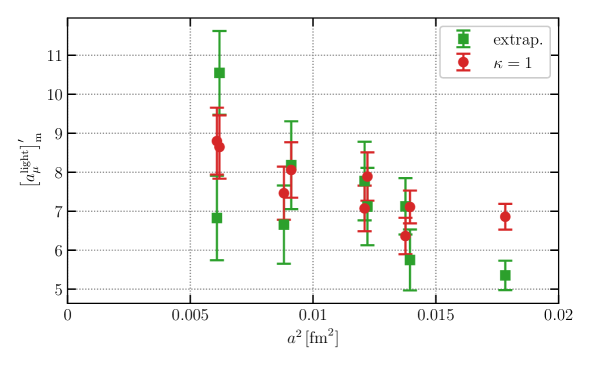
Figure 8: Strong-isospin-breaking (SIB) contribution to $a_{\mu}^{\text{light}}$. The green squares show the results from [52], obtained through a chiral extrapolation from measurements performed at valence quark masses which are $\kappa=3,5,7$ times larger than the physical light quark mass $m_{l}$. The red circles correspond to the measurements performed directly at $\kappa=1$ using a LMA-based technique.

In case of the valence QED contribution $[a_{\mu}^{\mathrm{light}}]^{\prime\prime}_{20}$, we have checked the gauge-configuration by gauge-configuration extrapolation procedure on one selected configuration. We have randomly chosen one QCD and QED configuration from one of our $a=0.0787\,\mathrm{fm}$ ensembles, and measured the valence QED contribution using the LMA technique. For the exact eigen part we projected out 4128 eigenvectors, and used 36000 random source vectors for the $\kappa=3,5,7$ measurements, and 72000 random source vectors for the $\kappa=1$ measurement. Figure 9 shows $[a_{\mu}^{\mathrm{light}}]^{\prime\prime}_{20}$ as the function of the time cut $t_{c}$, the upper limit of the integration of the Euclidean time current-current correlator.

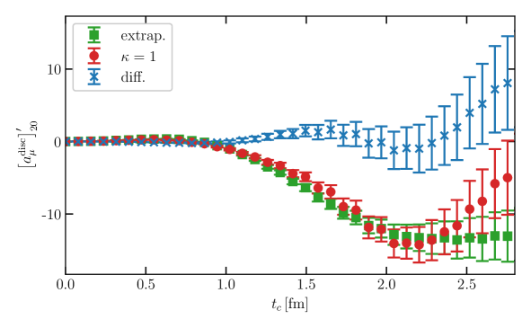
Figure 9: The valence QED contribution $[a_{\mu}^{\mathrm{light}}]^{\prime\prime}_{20}$ on a selected $a=0.0787\,\mathrm{fm}$ configuration, as the function of the upper limit of the time integration $t_{c}$. The green squares show the results obtained through a chiral extrapolation from measurements performed at valence quark masses which are $\kappa=3,5,7$ times larger than the physical light quark mass $m_{l}$. The red circles correspond to the measurements performed directly at $\kappa=1$, and the blue crosses show the difference of the two methods.

7.2 Strong-isospin-breaking contribution to $a_{\mu}^{\mathrm{disc}}$

In our previous work [52] the SIB contribution to $a_{\mu}^{\mathrm{disc}}$ was computed by performing a numerical derivative: the mass derivative was approximated by the difference of the measurements at the light quark masses $1.0\cdot m_{l}$ and $0.9\cdot m_{l}$. Using the recently developed frequency-splitting estimator (FSE) technique of Ref. [93], we have remeasured on many of our ensembles both the disconnected contribution to $a_{\mu}$, and its SIB contribution as an exact mass derivative. By using the FSE method, the number of required random source vectors drops by one to two orders of magnitude. A comparison of the new FSE measurements of $[a_{\mu}^{\mathrm{disc}}]^{\prime}_{m}$ and the results from [52] is shown in Figure 10.

Figure 10: Strong-isospin-breaking (SIB) contribution to $a_{\mu}^{\text{disc}}$. The green squares show the data points obtained using the finite difference method of Ref. [52], with 3000 random source vectors. The red circles are obtained using the FSE technique of Giusti et. al. [93], with 128 random source vectors.

7.3 Corrections

We discovered two mistakes in our 2020 work, which affect the isopsin-breaking contributions. None of them was numerically important for $a_{\mu}$, in the sense that the associated changes are far less than our final uncertainty.

First, we did set too aggressive time-cuts for the light quark sea QED contribution, $[a_{\mu}^{\mathrm{light}}]^{{}^{\prime\prime}}_{02}$. We used $1.0~{}\mathrm{fm}$ and $1.5~{}\mathrm{fm}$, which are not yet in the plateau region. An appropriate choice, $2.2~{}\mathrm{fm}$ and $2.7~{}\mathrm{fm}$, decreases the contribution significantly and the values in Figure 1 of the main text and in Table 15 of the Supplemental Information in [52] have to be changed as follows:

$$\text{light qed:}\quad-0.93(35)(47)\to-1.57(42)(35)$$ (45)

$$\text{light qed-ss:}\quad 0.37(21)(24)\to-0.36(27)(15)$$ (46)

In addition, we mistakenly subtracted a term related to one-photon-reducible contributions, $a_{\mu}^{1\gamma R}$, that we computed by means of infinite volume QED. For consistency with our lattice setup, this term should also be computed in QED_L. Due to the zero-spatial momentum projection of the correlation function the spatial momentum of the photon vanishes. However, in the QED_L prescription these particular modes are removed from the theory such that this subtraction is identically zero. Therefore in Table 16 of [52] the following change

$$\text{one-photon-reducible subtraction:}\quad-0.321(11)\to 0$$ (47)

has to be applied.

Regarding the total $a_{\mu}$, we keep using the originally published number as our 2020 result, when we refer to it in this paper. As we mentioned, fixing the two mistakes would change $a_{\mu}$ only by a small fraction of its total error. In the new numbers of this work, these mistakes are of course corrected.

8 Data-driven determination of finite-volume corrections

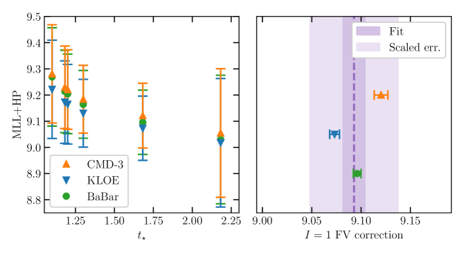
Figure 11: Results for data-driven determination of finite-volume effects in the $00-28$ window. The left panel shows, on the y-axis, the sum of the MLL and HP (1-pion and regular) contributions to the $I=1$ finite-volume correction, obtained using fits to the different experimental data sets, as a function of the time $t_{\star}$ at which we switch from HP to MLL. On top of the smaller error due to the fit parameters, the uncertainty reported here accounts for the truncation of either series and for the one associated with the regular part of HP, as described in the main text. The right panel contains again $I=1$ finite-volume corrections from individual data sets, but the uncertainty purely comes from the fit parameters that determine the phase shift. On the same plot the weighted average is shown as a purple dashed vertical line and the inner and outer bands respectively correspond to the uncertainties, without and with the multiplicative factor of $\sqrt{\chi^{2}/\mathrm{dof}}$ described in the text.

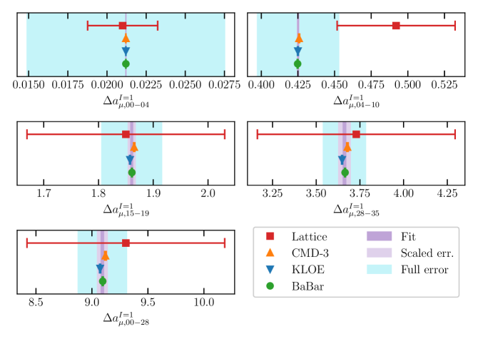
Figure 12: Comparison of results for the $I=1$ finite-volume correction in various windows. The red points correspond to the 4hex lattice results. The other points correspond to the data-driven determinations from individual data sets. Their averages are also displayed (inner two bands), as described in Figure 11. Finally, the outer band displays the total uncertainty on our data-driven determination, accounting for the systematic effects described in this section.

Using a data-driven approach, in this section we compute the finite-volume corrections to the various isovector window observables considered in this paper. We generically denote them $\Delta a_{\mu}^{\mathrm{I=1}}(L_{\rm ref}\rightarrow\infty)$. We employ a combination of the Meyer-Lellouch-Lüscher [94, 95, 96] (MLL) and the Hansen-Patella [97, 98] (HP) methods. They allow the calculation of finite-volume corrections from the infinite-volume $\pi\pi$ elastic phase shift $\delta_{11}$ in the $I^{G}(J^{PC})=1^{+}(1^{{--}})$ channel. The methods additionally require the $I=1$ component of the pion electromagnetic form factor $F_{\pi}^{I=1}(s)$, evaluated in the timelike domain $s>0$ for MLL and in the spacelike region $s\leq 0$ for HP.

The MLL formalism has been widely used with the Gounaris-Sakurai parametrization [99] of the form factor and the phase shift. We adopt instead a data-driven approach based on the parametrization of Ref. [100, 101, 102]. The corresponding parameters are obtained via new individual fits to three measurements of the $e^{+}e^{-}\to\pi^{+}\pi^{-}$ spectra by BaBar [103, 104], CMD-3 [105] and KLOE [106, 107, 108, 109], according to the procedure described in Ref. [102]. For each data set we then obtain the phase shift $\delta_{11}(s)$ and the form factor,

$$F^{I=1}_{\pi}(s)=J(s)\Omega(s)\;,$$ (48)

where $\Omega(s)$ is the Omnès function [110],

$$\Omega(s)=\exp\frac{s}{\pi}\int_{s_{\rm th}}^{\infty}ds^{\prime}\,\frac{\delta_{11}(s^{\prime})}{s^{\prime}(s^{\prime}-s)}\,,$$ (49)

and $J(s)=1+\alpha_{V}s$, where $\alpha_{V}$ is one of the fit parameters. Equation (48) corresponds to the $I=1$ component of the pion form factor, up to inelastic contributions.

Following Ref. [52], for MLL eight finite-volume states are used to construct the finite-volume correlator $G(t,L)$, an approximation that is increasingly accurate at larger Euclidean times $t$. The last, eighth term is taken as an estimate of the uncertainty due to the truncation of the sum over states. It is added to the finite-volume correlator with a 100% uncertainty. To keep this uncertainty small and its estimate reliable, we use MLL only at times larger than $t_{\star}=(M_{\pi}L/4)^{2}/M_{\pi}$, as suggested in Ref. [111].

Below $t_{\star}$, where MLL poorly represents the finite-volume correlator, the HP series of Ref. [98] is used, including the three terms that have been computed, thus neglecting contributions of order $\exp\left(-M_{\pi}L\sqrt{2+\sqrt{3}}\right)$ and higher. The last, third term is used as an estimate of the uncertainty due to the truncation of the series. The calculation of these terms requires knowledge of the Compton scattering amplitude of a pion off a spacelike photon. As shown in Ref. [98] this is dominated by the exchange of a single pion. This is in turn related to the spacelike pion form factor, for which we use again Equation (49). The result for the HP single pion term is then added to the MLL contribution. Their uncertainties are summed assuming 100% correlation, since they derive from the same phase shift.

The rest of the Compton amplitude was computed in NLO XPT in Ref. [98]. We adopt the same expression, which amounts to a small contribution to the result, called “regular part”, to which we assign a 100% uncertainty that is combined in quadrature with the other uncertainties. Results for the combination of MLL and HP are listed in Table 15 for the windows of interest in this paper.

The choice of $t_{\star}$ should not be critical as long as one does not use MLL at short distances, or HP at long distances, where the methods are not reliable. We have checked the dependence of our result on different values of $t_{\star}$. We find compatibility within the uncertainties, provided we do not consider large or small values of $t_{\star}$, as shown in the left panel of Figure 11 where we scan around $t_{\star}=1.682\,\mathrm{fm}$, using the $00-28$ window as an example.

Another potential source of systematic uncertainty is the inelastic contribution to $F_{\pi}^{I=1}(s)$ due to four-pion states. Given that inelasticities become sizable only at energies around $M_{\omega}+M_{\pi}$ [112], one would expect them not to propagate significantly into the finite-volume correction to $a_{\mu}$. We note that XPT predicts that they begin at order $s^{3}$. In the chiral regime, $s^{3}$ is two orders higher than the linear $s$ term in $J(s)$. Thus we conservatively take the effect of that linear term as an estimate of the possible size of such higher-order contributions. This is achieved by repeating our calculation of the finite-volume corrections without that linear term in $J(s)$. This results in a small shift in the finite-volume corrections, which we take as an additional systematic.

While we use the phase shift in the isospin limit, where we identify the pion mass with $M_{\pi^{0}}$, our parametrization of the phase shift is fitted to experimental data, where the pions are charged. We regard this as an isospin-breaking effect in the finite-volume corrections. In order to estimate this effect, we adopt the two-loop inverse-amplitude-method (IAM) expression of $\delta_{11}(s)$ from Ref. [113], which has the advantage of displaying dependence on the pion mass. By using the inputs for the IAM provided in Ref. [112, 114], we perform our calculation with the phase shift at the mass of neutral and of charged pions. The resulting shifts in the finite-volume corrections are taken as estimates of this additional source of uncertainty. We consider this effect to be independent of the other systematics and we add it to them in quadrature.

Finally, we need to propagate the uncertainties from the fits to BaBar, KLOE and CMD-3. To this end we generate Gaussian samples for the fit parameters associated with each experimental data set. While the parameters associated with different experiments are not correlated, they are correlated for a given data set. We account for those correlations and compute the standard deviations on the resulting finite-volume corrections. With this procedure, before including the various systematic uncertainties described above, the finite-volume correction determined from CMD-3 data is not compatible with the one coming from fits to BaBar and KLOE data. Since the data sets are independent, we compute an average of the corresponding finite-volume corrections, each weighted by its uncertainty. The result is reported in the right panel of Figure 11. Given the discrepancy between individual points, we considered the difference between KLOE and CMD3 as a systematic or, instead, rescaling the uncertainty by $\sqrt{\chi^{2}/\mathrm{dof}}$. This choice does not crucially determine our final uncertainty, which is dominated by other systematics, and we opt for the larger of the two uncertainties, i.e. the rescaling by $\sqrt{\chi^{2}/\mathrm{dof}}$. We report this result for the $00-28$ window in the same figure.

The various sources of uncertainties on the finite-volume corrections studied here are listed in Table 16: truncation, regular part of HP, inelastic, tension between experiments and isospin breaking. They are assumed to be independent and are summed in quadrature. Truncation, inelastic and isospin uncertainties are computed for each data set and we only keep the largest value for each source of uncertainty. The result of this combination is shown for each window in Table 16, which contains our complete data-driven determinations of the finite-volume corrections. We find them to be in agreement with the corresponding values computed using the 4hex simulations. In Figure 12 we update the right panel of Figure 11 to include the full uncertainty and a comparison with the corresponding 4hex value, and we display results for all windows.

window	MLL	HP(1-pion)	HP(regular)	sum
$00-28$	$6.60(0.02)$	$2.43(0.09)$	$0.06(0.06)$	$9.09(0.12)$
$00-04$	$0.00(0.00)$	$0.01(0.00)$	$0.01(0.01)$	$0.02(0.01)$
$04-10$	$0.00(0.00)$	$0.40(0.01)$	$0.02(0.02)$	$0.43(0.03)$
$15-19$	$1.13(0.01)$	$0.72(0.03)$	$0.01(0.01)$	$1.86(0.04)$
$28-35$	$3.66(0.00)$	$0.00(0.00)$	$0.00(0.00)$	$3.66(0.00)$

Table 15: Results for the HP and MLL contributions in the windows of interest in this paper. HP is used to compute the finite-volume corrections to $a_{\mu}^{\mathrm{I=1}}$, integrating the correlator from $t=0$ up to $t_{\star}=1.682\,\mathrm{fm}$. It is divided into the single pion contribution, reported in the third column, and the regular part, in the fourth column. From $t_{\star}$ to infinity, MLL is used. The uncertainty on the sum, reported in the last column, assumes 100% correlation between the uncertainties on MLL and HP (1-pion). The uncertainty attached to the regular part of HP is added in quadrature.

window	trunc. (MLL+HP)	HP(regular)	inel.	exp.	iso.	quad. sum
$00-28$	$0.11$	$0.06$	$0.14$	$0.04$	$0.10$	$0.22$
$00-04$	$0.00$	$0.01$	$0.00$	$0.00$	$0.00$	$0.01$
$04-10$	$0.01$	$0.02$	$0.00$	$0.00$	$0.01$	$0.03$
$15-19$	$0.04$	$0.01$	$0.03$	$0.01$	$0.02$	$0.06$
$28-35$	$0.00$	$0.00$	$0.10$	$0.03$	$0.06$	$0.12$

Table 16: Uncertainties in the finite-volume corrections to $a_{\mu}^{\mathrm{I=1}}$ in the windows of interest in this paper. The numbers reported correspond to the data set (BaBar, KLOE or CMD-3) that has the largest uncertainty for the given entry. The second column is the sum of the truncation uncertainties of HP and MLL, which are assumed to be 100% correlated. The third column is due to the 100% uncertainty on the leftover regular part of HP. The fourth column is the difference between the finite-volume correction result, with and without the inelastic contribution to the pion form factor. The fifth column shows the weighted average over experiments, inflated by $\sqrt{\chi^{2}/\mathrm{dof}}$. In the sixth column, we report an estimate of isospin-breaking effects. The last column contains the sum in quadrature of all these contributions.

window	$\Delta a_{\mu}^{I=1}(L_{\rm ref}\rightarrow\infty)$
$00-28$	$9.09(0.22)$
$00-04$	$0.02(0.01)$
$04-10$	$0.43(0.03)$
$15-19$	$1.86(0.06)$
$28-35$	$3.66(0.12)$

Table 17: Results for the finite-volume corrections on $a_{\mu}^{\mathrm{I=1}}$ in the windows of interest in this paper, accounting for the uncertainties described in the main body of the section.

9 Long-distance contributions

As emphasized in the main text, our goal is to compute the leading-order hadronic vacuum polarization contribution to the anomalous magnetic moment of the muon, with fully controlled uncertainties that are significantly smaller than available today.

The vast majority of our final result (over $95\%$) comes directly from lattice simulations. However, there is a contribution for which a data-driven approach yields an order of magnitude smaller uncertainty than a lattice calculation. It is the one corresponding to the large Euclidean-time “tail” of the current correlator. We choose it to correspond to a window [79] that extends from $2.8\,\mathrm{fm}$ to $\infty$, for reasons explained below. We denote it $a_{\mu,28-\infty}$. Another set of contributions for which a data-driven approach can lead to uncertainty reduction is the one corresponding to finite-volume corrections, as discussed in Section 8.

Before going into the details of how this tail contribution is obtained, it is important to clarify a number of issues. As is well known, the reference data-driven determination of the full LO-HVP contribution leads to significant tensions between the standard-model prediction [115] and the experimentally measured value of $(g_{\mu}-2)$ [116]. In addition, our previous lattice determination of $a_{\mu}$ is $2.1\sigma$ larger than the reference one [115], a tension that rises to over $4\sigma$ when one considers the intermediate-distance window contribution $a_{\mu,04-10}$ [117, 83]. To make the situation even more confusing, the recent measurement of the $e^{+}e^{-}\to\pi^{+}\pi^{-}$ spectrum by the CMD-3 collaboration leads to predictions for $a_{\mu}$ and for $a_{\mu,04-10}$ that are in good agreement with our 2020 lattice ones [118].

In that last reference [118], some of us reappraised the data-driven determination of $a_{\mu}$, showing that results, based on measurements of the $\pi^{+}\pi^{-}$ spectrum by BaBar [103, 104], CMD-3 [105], KLOE[106, 107, 108, 109] and via hadronic $\tau$ decays [119, 120], display significant tensions. This reappraisal was prompted by a detailed study of radiative corrections in initial-state radiation measurements, which suggests that KLOE may have underestimated its systematic uncertainties on the $\rho$ peak [121].

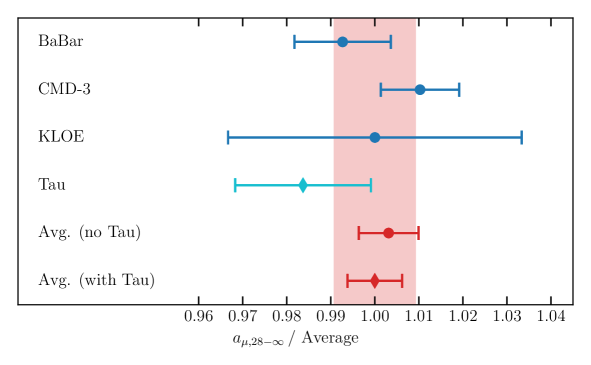
Figure 13: Results for $a_{\mu,28-\infty}$ obtained using the $\pi^{+}\pi^{-}$ spectra measured by BaBar, KLOE, CMD-3 and in $\tau$ decays. The results are normalized by their weighted average, which is shown by a red diamond in the bottom. Above that, the red circle shows the weighted average without the $\tau$ data. Neither of these needed a PDG rescaling of the error. The red band represents the total uncertainty, which is obtained by adding linearly the error of the weighted average of all data and the difference of the two types of averages.

In light of those challenges, one may wonder whether it is justified to consider a data-driven determination of $a_{\mu,28-\infty}$. To understand why it is, we emphasize a few important facts:

• As shown in Figure 13, the determinations of this tail contribution, using the $\pi^{+}\pi^{-}$ spectrum from each of the four experiments, are entirely consistent. The $\chi^{2}/\mathrm{dof}$ associated with the weighted average of those four determinations is $1.0$. The reason is that the tail contribution is dominated by the low-mass part of the spectrum, below the $\rho$ peak, where all four measurements are in good agreement.

• We have checked that the data-driven contribution to $a_{\mu}$ from $t\geq 2.8\,\mathrm{fm}$ is entirely compatible with our lattice calculation. This is shown in Figure 14 where we compare results for the window $28-35$ obtained from the four measurements and in lattice QCD. Here again the data-driven determinations are entirely compatible among themselves, with a $\chi^{2}/\mathrm{dof}$ of $1.2$, and now with the lattice result. Admittedly the uncertainties on the latter are large, but the excellent consistency with and of the four data-driven determinations strongly suggests that the data-driven calculation of $a_{\mu,28-\infty}$ is correct, within our quoted uncertainties.

• The total uncertainty on our average of the data-driven $a_{\mu,28-\infty}$ is $0.20$ in our $10^{-10}$ units, a number that must be compared to our total uncertainty of $3.3$ on $a_{\mu}$. Thus its impact on the uncertainty of our final result for $a_{\mu}$ is completely negligible.

Now, the reasons for choosing the tail to start at $t_{\mathrm{cut}}=2.8~{}\mathrm{fm}$ are the following:

• To ensure the result for $a_{\mu}$ presented in this paper is dominated by the lattice contribution, we choose to start the data-driven tail above $t=2.8\,\mathrm{fm}$. This guarantees that the lattice contribution accounts for over $95\%$ of the result.

• Beyond reducing the uncertainty on $a_{\mu,28-\infty}$ by an order of magnitude, the use of a data-driven tail reduces the finite-volume correction that must be applied to the lattice result by a factor of $2$ and the associated uncertainty by even more.

• As discussed above, for these large times the data-driven determinations of $a_{\mu,28-\infty}$ agree very well.

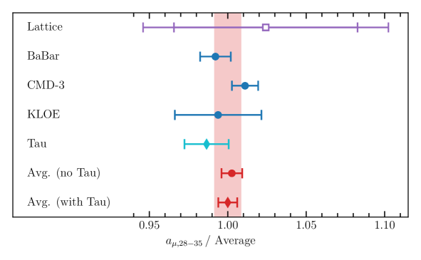
Figure 14: Results for $a_{\mu,28-35}$. Figure description is the same as in Figure 13. Additionally, the purple square on the top represents our lattice result, which is in excellent agreement with the data-driven determinations. In the weighted averages on the bottom, a small PDG rescaling of the error was applied.

Having justified the use of a data-driven approach for determining the tail contribution, we now explain briefly how it is calculated. As mentioned above, the computation is performed following the approach of Ref. [118]. In that work, the measurements of the $\pi^{+}\pi^{-}$ spectrum by BaBar [103, 104], KLOE [106, 107, 108, 109], CMD-3 [105] and via hadronic $\tau$ decays [119, 120] are considered separately. Outside their center-of-mass energy ranges and for other hadronic channels, the data from each experiment are complemented by the combined experimental and perturbative QCD results compiled in Ref. [102, 120], with a full treatment of uncertainties and correlations. For BaBar and $\tau$ decays, center-of-mass energies range from $0.3\,\mathrm{Ge\kern-1.00006ptV}$ and $2M_{\pi^{\pm}}$ to $1.8\,\mathrm{Ge\kern-1.00006ptV}$, and for CMD-3, $0.33\,\mathrm{Ge\kern-1.00006ptV}$ up to $1.2\,\mathrm{Ge\kern-1.00006ptV}$. KLOE covers the range from $0.32\,\mathrm{Ge\kern-1.00006ptV}$ to $0.97\,\mathrm{Ge\kern-1.00006ptV}$.

The HVPTools framework [122, 123, 124, 102] is then used to Laplace transform [125] these four spectra into the corresponding Euclidean-time correlators. The latter are subsequently integrated, with the window weights of Ref. [79], to give the four data-driven results for $a_{\mu,28-\infty}$. As discussed above, the tail contributions are shown in Figure 13 and the comparison of results for the $28-35$ window in Figure 14.

To obtain our final results for the tail and the $28-35$ window contributions, we perform weighted averages of the BaBar, KLOE and CMD-3 and $\tau$-decay determinations, taking into account all correlations. This procedure yields our final central values for those quantities, as well as the uncertainties originating from those in the cross sections.

The agreement of the results using the different data sets is excellent. Nonetheless, we apply the PDG [126] $\sqrt{\chi^{2}/\mathrm{dof}}$ error-rescaling factor in the case of the $28-35$ window, which has a $\chi^{2}/\mathrm{dof}$ only slightly larger than 1. The $\chi^{2}/\mathrm{dof}$ for $a_{\mu,28-\infty}$ is less than 1.

The agreement between the results obtained using different data sets fully extends to those determined via $\tau$ data. The use of $\tau$ data in this context requires that one estimates isospin-breaking corrections. This was done very carefully in Ref. [119]. Nevertheless, we conservatively consider the absolute value of the full difference between the averages, obtained with and without the $\tau$-decay data, as an additional uncertainty. We add it linearly to the other uncertainties. In that way, our error bar necessarily covers the average in which only $e^{+}e^{-}$ data are used. For both quantities studied in the present section this additional uncertainty is smaller than the one induced by those in the cross sections.

Altogether, we obtain

$$a_{\mu,28-\infty}=27.59(17)(9)[26]\quad\text{and}\quad a_{\mu,28-35}=18.12(11)(5)[16]$$ (50)

for our tail-related window results in the data-driven approach. The first error comes from the weighted average procedure of different experiments and includes a PDG-style error rescaling. The second error is the additional uncertainty from including or not including the $\tau$ data set. The third, conservative total error is the first two added linearly.

References

- [1] D.. Aguillard “Measurement of the Positive Muon Anomalous Magnetic Moment to 0.20 ppm” In Phys. Rev. Lett. 131.16, 2023, pp. 161802 DOI: 10.1103/PhysRevLett.131.161802
- [2] T. Aoyama “The anomalous magnetic moment of the muon in the Standard Model” In Phys. Rept. 887, 2020, pp. 1–166 DOI: 10.1016/j.physrep.2020.07.006
- [3] Sz. Borsanyi “Leading hadronic contribution to the muon magnetic moment from lattice QCD” In Nature 593.7857, 2021, pp. 51–55 DOI: 10.1038/s41586-021-03418-1
- [4] F.. Ignatov “Measurement of the e+e-→+- cross section from threshold to 1.2 GeV with the CMD-3 detector” In Phys. Rev. D 109.11, 2024, pp. 112002 DOI: 10.1103/PhysRevD.109.112002
- [5] Fred Jegerlehner and Andreas Nyffeler “The Muon g-2” In Phys. Rept. 477, 2009, pp. 1–110 DOI: 10.1016/j.physrep.2009.04.003
- [6] David Bernecker and Harvey B. Meyer “Vector Correlators in Lattice QCD: Methods and applications” In Eur. Phys. J. A47, 2011, pp. 148 DOI: 10.1140/epja/i2011-11148-6
- [7] B.. Lautrup, A. Peterman and E. Rafael “Recent developments in the comparison between theory and experiments in quantum electrodynamics” In Phys. Rept. 3, 1972, pp. 193–259 DOI: 10.1016/0370-1573(72)90011-7
- [8] Eduardo Rafael “Hadronic contributions to the muon g-2 and low-energy QCD” In Phys. Lett. B322, 1994, pp. 239–246 DOI: 10.1016/0370-2693(94)91114-2
- [9] T. Blum “Lattice calculation of the lowest order hadronic contribution to the muon anomalous magnetic moment” In Phys. Rev. Lett. 91, 2003, pp. 052001 DOI: 10.1103/PhysRevLett.91.052001
- [10] Sz. Borsanyi “Hadronic vacuum polarization contribution to the anomalous magnetic moments of leptons from first principles” In Phys. Rev. Lett. 121.2, 2018, pp. 022002 DOI: 10.1103/PhysRevLett.121.022002
- [11] M. Davier et al. “Reevaluation of the hadronic contribution to the muon magnetic anomaly using new e+ e- — pi+ pi- cross section data from BABAR” In Eur. Phys. J. C 66, 2010, pp. 1–9 DOI: 10.1140/epjc/s10052-010-1246-1
- [12] Michel Davier, Andreas Hoecker, Bogdan Malaescu and Zhiqing Zhang “Reevaluation of the Hadronic Contributions to the Muon g-2 and to alpha(MZ)” [Erratum: Eur.Phys.J.C 72, 1874 (2012)] In Eur. Phys. J. C 71, 2011, pp. 1515 DOI: 10.1140/epjc/s10052-012-1874-8
- [13] Michel Davier, Andreas Hoecker, Bogdan Malaescu and Zhiqing Zhang “Reevaluation of the hadronic vacuum polarisation contributions to the Standard Model predictions of the muon and using newest hadronic cross-section data” In Eur. Phys. J. C77.12, 2017, pp. 827 DOI: 10.1140/epjc/s10052-017-5161-6
- [14] M. Davier, A. Hoecker, B. Malaescu and Z. Zhang “A new evaluation of the hadronic vacuum polarisation contributions to the muon anomalous magnetic moment and to ” In Eur. Phys. J. C 80.3, 2020, pp. 241 DOI: 10.1140/epjc/s10052-020-7792-2
- [15] Bernard Aubert “Precise measurement of the e+ e- — pi+ pi- (gamma) cross section with the Initial State Radiation method at BABAR” In Phys. Rev. Lett. 103, 2009, pp. 231801 DOI: 10.1103/PhysRevLett.103.231801
- [16] J.. Lees “Precise Measurement of the Cross Section with the Initial-State Radiation Method at BABAR” In Phys. Rev. D 86, 2012, pp. 032013 DOI: 10.1103/PhysRevD.86.032013
- [17] F. Ambrosino “Measurement of and the dipion contribution to the muon anomaly with the KLOE detector” In Phys. Lett. B 670, 2009, pp. 285–291 DOI: 10.1016/j.physletb.2008.10.060
- [18] F. Ambrosino “Measurement of from threshold to 0.85 GeV2 using Initial State Radiation with the KLOE detector” In Phys. Lett. B 700, 2011, pp. 102–110 DOI: 10.1016/j.physletb.2011.04.055
- [19] D. Babusci “Precision measurement of and determination of the contribution to the muon anomaly with the KLOE detector” In Phys. Lett. B 720, 2013, pp. 336–343 DOI: 10.1016/j.physletb.2013.02.029
- [20] A. Anastasi “Combination of KLOE measurements and determination of in the energy range GeV2” In JHEP 03, 2018, pp. 173 DOI: 10.1007/JHEP03(2018)173
- [21] M. Davier et al. “The Discrepancy Between tau and e+e- Spectral Functions Revisited and the Consequences for the Muon Magnetic Anomaly” In Eur. Phys. J. C 66, 2010, pp. 127–136 DOI: 10.1140/epjc/s10052-009-1219-4
- [22] Michel Davier et al. “Update of the ALEPH non-strange spectral functions from hadronic decays” In Eur. Phys. J. C 74.3, 2014, pp. 2803 DOI: 10.1140/epjc/s10052-014-2803-9
- [23] M. Davier et al. “Tensions in measurements: the new landscape of data-driven hadronic vacuum polarization predictions for the muon ”, 2023 arXiv:2312.02053 [hep-ph]
- [24] Christopher Aubin et al. “Light quark vacuum polarization at the physical point and contribution to the muon ” In Phys. Rev. D 101.1, 2020, pp. 014503 DOI: 10.1103/PhysRevD.101.014503
- [25] Harvey B. Meyer “Lattice QCD and the Timelike Pion Form Factor” In Phys. Rev. Lett. 107, 2011, pp. 072002 DOI: 10.1103/PhysRevLett.107.072002
- [26] Laurent Lellouch and Martin Luscher “Weak transition matrix elements from finite volume correlation functions” In Commun. Math. Phys. 219, 2001, pp. 31–44 DOI: 10.1007/s002200100410
- [27] Martin Luscher “Two particle states on a torus and their relation to the scattering matrix” In Nucl. Phys. B354, 1991, pp. 531–578 DOI: 10.1016/0550-3213(91)90366-6
- [28] Maxwell T. Hansen and Agostino Patella “Finite-volume effects in ” In Phys. Rev. Lett. 123, 2019, pp. 172001 DOI: 10.1103/PhysRevLett.123.172001
- [29] Maxwell T. Hansen and Agostino Patella “Finite-volume and thermal effects in the leading-HVP contribution to muonic ()” In JHEP 10, 2020, pp. 029 DOI: 10.1007/JHEP10(2020)029
- [30] T. Blum et al. “Calculation of the hadronic vacuum polarization contribution to the muon anomalous magnetic moment” In Phys. Rev. Lett. 121.2, 2018, pp. 022003 DOI: 10.1103/PhysRevLett.121.022003
- [31] Genessa Benton et al. “Data-Driven Determination of the Light-Quark Connected Component of the Intermediate-Window Contribution to the Muon g-2” In Phys. Rev. Lett. 131.25, 2023, pp. 251803 DOI: 10.1103/PhysRevLett.131.251803
- [32] T. Blum “Update of Euclidean windows of the hadronic vacuum polarization” In Phys. Rev. D 108.5, 2023, pp. 054507 DOI: 10.1103/PhysRevD.108.054507
- [33] Christoph Lehner and Aaron S. Meyer “Consistency of hadronic vacuum polarization between lattice QCD and the R-ratio” In Phys. Rev. D 101, 2020, pp. 074515 DOI: 10.1103/PhysRevD.101.074515
- [34] Gen Wang, Terrence Draper, Keh-Fei Liu and Yi-Bo Yang “Muon g-2 with overlap valence fermions” In Phys. Rev. D 107.3, 2023, pp. 034513 DOI: 10.1103/PhysRevD.107.034513
- [35] Christopher Aubin, Thomas Blum, Maarten Golterman and Santiago Peris “Muon anomalous magnetic moment with staggered fermions: Is the lattice spacing small enough?” In Phys. Rev. D 106.5, 2022, pp. 054503 DOI: 10.1103/PhysRevD.106.054503
- [36] Marco Cè “Window observable for the hadronic vacuum polarization contribution to the muon g-2 from lattice QCD” In Phys. Rev. D 106.11, 2022, pp. 114502 DOI: 10.1103/PhysRevD.106.114502
- [37] C. Alexandrou “Lattice calculation of the short and intermediate time-distance hadronic vacuum polarization contributions to the muon magnetic moment using twisted-mass fermions” In Phys. Rev. D 107.7, 2023, pp. 074506 DOI: 10.1103/PhysRevD.107.074506
- [38] Alexei Bazavov “Light-quark connected intermediate-window contributions to the muon g-2 hadronic vacuum polarization from lattice QCD” In Phys. Rev. D 107.11, 2023, pp. 114514 DOI: 10.1103/PhysRevD.107.114514
- [39] Alexander Keshavarzi, Daisuke Nomura and Thomas Teubner “Muon and : a new data-based analysis” In Phys. Rev. D97.11, 2018, pp. 114025 DOI: 10.1103/PhysRevD.97.114025
- [40] Alexander Keshavarzi, Daisuke Nomura and Thomas Teubner “ of charged leptons, , and the hyperfine splitting of muonium” In Phys. Rev. D101.1, 2020, pp. 014029 DOI: 10.1103/PhysRevD.101.014029
- [41] J.. Lees “Measurement of additional radiation in the initial-state-radiation processes e+e-→+- and e+e-→+- at BABAR” In Phys. Rev. D 108.11, 2023, pp. L111103 DOI: 10.1103/PhysRevD.108.L111103
- [42] Simon Kuberski et al. “Hadronic vacuum polarization in the muon g 2: the short-distance contribution from lattice QCD” In JHEP 03, 2024, pp. 172 DOI: 10.1007/JHEP03(2024)172
- [43] G. Colangelo “Prospects for precise predictions of in the Standard Model” Contribution to the 2020-2022 Particle Physics Community Planning Exercise (a.k.a. “Snowmass”) process organised by the Division of Particles and Fields (DPF) of the American Physical Society., 2022 arXiv:2203.15810 [hep-ph]
- [44] C.. Carloni Calame, M. Passera, L. Trentadue and G. Venanzoni “A new approacwh to evaluate the leading hadronic corrections to the muon -2” In Phys. Lett. B746, 2015, pp. 325–329 DOI: 10.1016/j.physletb.2015.05.020
- [45] Michel Davier et al. “Hadronic vacuum polarization: Comparing lattice QCD and data-driven results in systematically improvable ways” In Phys. Rev. D 109.7, 2024, pp. 076019 DOI: 10.1103/PhysRevD.109.076019
- [46] www.gauss-centre.eu
- [47] www.genci.fr/en
- [48] M. Luscher and P. Weisz “On-Shell Improved Lattice Gauge Theories” [Erratum: Commun. Math. Phys.98,433(1985)] In Commun. Math. Phys. 97, 1985, pp. 59 DOI: 10.1007/BF01206178
- [49] Colin Morningstar and Mike J. Peardon “Analytic smearing of SU(3) link variables in lattice QCD” In Phys. Rev. D69, 2004, pp. 054501 DOI: 10.1103/PhysRevD.69.054501
- [50] C. McNeile et al. “High-Precision c and b Masses, and QCD Coupling from Current-Current Correlators in Lattice and Continuum QCD” In Phys. Rev. D 82, 2010, pp. 034512 DOI: 10.1103/PhysRevD.82.034512
- [51] Y. Aoki “FLAG Review 2021” In Eur. Phys. J. C 82.10, 2022, pp. 869 DOI: 10.1140/epjc/s10052-022-10536-1
- [52] Sz. Borsanyi “Leading hadronic contribution to the muon magnetic moment from lattice QCD” In Nature 593.7857, 2021, pp. 51–55 DOI: 10.1038/s41586-021-03418-1
- [53] M.. Clark and A.. Kennedy “Accelerating dynamical fermion computations using the rational hybrid Monte Carlo (RHMC) algorithm with multiple pseudofermion fields” In Phys. Rev. Lett. 98, 2007, pp. 051601 DOI: 10.1103/PhysRevLett.98.051601
- [54] Hantao Yin and Robert D. Mawhinney “Improving DWF Simulations: the Force Gradient Integrator and the Möbius Accelerated DWF Solver” In PoS LATTICE2011, 2011, pp. 051 DOI: 10.22323/1.139.0051
- [55] J.. Sexton and D.. Weingarten “Hamiltonian evolution for the hybrid Monte Carlo algorithm” In Nucl. Phys. B 380, 1992, pp. 665–677 DOI: 10.1016/0550-3213(92)90263-B
- [56] Martin Hasenbusch “Speeding up the hybrid Monte Carlo algorithm for dynamical fermions” In Phys. Lett. B 519, 2001, pp. 177–182 DOI: 10.1016/S0370-2693(01)01102-9
- [57] Fabian Joswig, Simon Kuberski, Justus T. Kuhlmann and Jan Neuendorf “pyerrors: A python framework for error analysis of Monte Carlo data” In Comput. Phys. Commun. 288, 2023, pp. 108750 DOI: 10.1016/j.cpc.2023.108750
- [58] N. Ishizuka et al. “Operator dependence of hadron masses for Kogut-Susskind quarks on the lattice” In Nucl. Phys. B411, 1994, pp. 875–902 DOI: 10.1016/0550-3213(94)90475-8
- [59] A. Bazavov “ from decay and four-flavor lattice QCD” In Phys. Rev. D 99.11, 2019, pp. 114509 DOI: 10.1103/PhysRevD.99.114509
- [60] Maarten F.. Golterman and Jan Smit “Lattice Baryons With Staggered Fermions” In Nucl. Phys. B255, 1985, pp. 328–340 DOI: 10.1016/0550-3213(85)90138-5
- [61] Jon A. Bailey “Staggered baryon operators with flavor SU(3) quantum numbers” In Phys. Rev. D75, 2007, pp. 114505 DOI: 10.1103/PhysRevD.75.114505
- [62] S. Gusken et al. “Nonsinglet Axial Vector Couplings of the Baryon Octet in Lattice QCD” In Phys. Lett. B227, 1989, pp. 266–269 DOI: 10.1016/S0370-2693(89)80034-6
- [63] C. Aubin and K. Orginos “A new approach for Delta form factors” In Proceedings, 12th International Conference on Meson-nucleon physics and the structure of the nucleon (MENU 2000): Williamsburg, USA, May 31-June 4, 2010 1374.1, 2011, pp. 621–624 DOI: 10.1063/1.3647217
- [64] J. Yelton “Observation of an Excited Baryon” In Phys. Rev. Lett. 121.5, 2018, pp. 052003 DOI: 10.1103/PhysRevLett.121.052003
- [65] C.. Bouchard et al. “ form factors from lattice QCD” In Phys. Rev. D 90, 2014, pp. 054506 DOI: 10.1103/PhysRevD.90.054506
- [66] Mattia Bruno and Rainer Sommer “On fits to correlated and auto-correlated data” In Comput. Phys. Commun. 285, 2023, pp. 108643 DOI: 10.1016/j.cpc.2022.108643
- [67] Sz. Borsanyi “Isospin splittings in the light baryon octet from lattice QCD and QED” In Phys. Rev. Lett. 111.25, 2013, pp. 252001 DOI: 10.1103/PhysRevLett.111.252001
- [68] Johan Bijnens and Niclas Danielsson “Electromagnetic Corrections in Partially Quenched Chiral Perturbation Theory” In Phys. Rev. D75, 2007, pp. 014505 DOI: 10.1103/PhysRevD.75.014505
- [69] M. Di Carlo et al. “Light-meson leptonic decay rates in lattice QCD+QED” In Phys. Rev. D100.3, 2019, pp. 034514 DOI: 10.1103/PhysRevD.100.034514
- [70] Dominik Stamen et al. “Kaon electromagnetic form factors in dispersion theory” In Eur. Phys. J. C 82.5, 2022, pp. 432 DOI: 10.1140/epjc/s10052-022-10348-3
- [71] R. Horsley “QED effects in the pseudoscalar meson sector” In JHEP 04, 2016, pp. 093 DOI: 10.1007/JHEP04(2016)093
- [72] J. Gasser, A. Rusetsky and I. Scimemi “Electromagnetic corrections in hadronic processes” In Eur. Phys. J. C32, 2003, pp. 97–114 DOI: 10.1140/epjc/s2003-01383-1
- [73] D. Giusti et al. “Leading isospin-breaking corrections to pion, kaon and charmed-meson masses with Twisted-Mass fermions” In Phys. Rev. D 95.11, 2017, pp. 114504 DOI: 10.1103/PhysRevD.95.114504
- [74] W.. Cottingham “The neutron proton mass difference and electron scattering experiments” In Annals Phys. 25, 1963, pp. 424–432 DOI: 10.1016/0003-4916(63)90023-X
- [75] Nikolai Husung, Peter Marquard and Rainer Sommer “Asymptotic behavior of cutoff effects in Yang–Mills theory and in Wilson’s lattice QCD” In Eur. Phys. J. C 80.3, 2020, pp. 200 DOI: 10.1140/epjc/s10052-020-7685-4
- [76] William I. Jay and Ethan T. Neil “Bayesian model averaging for analysis of lattice field theory results” In Phys. Rev. D 103, 2021, pp. 114502 DOI: 10.1103/PhysRevD.103.114502
- [77] Peter Boyle et al. “Physical-mass calculation of and resonance parameters via and scattering amplitudes from lattice QCD”, 2024 arXiv:2406.19193 [hep-lat]
- [78] Sz. Borsanyi “Hadronic vacuum polarization contribution to the anomalous magnetic moments of leptons from first principles” In Phys. Rev. Lett. 121.2, 2018, pp. 022002 DOI: 10.1103/PhysRevLett.121.022002
- [79] T. Blum et al. “Calculation of the hadronic vacuum polarization contribution to the muon anomalous magnetic moment” In Phys. Rev. Lett. 121.2, 2018, pp. 022003 DOI: 10.1103/PhysRevLett.121.022003
- [80] T. Blum “Update of Euclidean windows of the hadronic vacuum polarization” In Phys. Rev. D 108.5, 2023, pp. 054507 DOI: 10.1103/PhysRevD.108.054507
- [81] Marco Cè et al. “Vacuum correlators at short distances from lattice QCD” In JHEP 12, 2021, pp. 215 DOI: 10.1007/JHEP12(2021)215
- [82] Simon Kuberski et al. “Hadronic vacuum polarization in the muon g 2: the short-distance contribution from lattice QCD” In JHEP 03, 2024, pp. 172 DOI: 10.1007/JHEP03(2024)172
- [83] C. Alexandrou “Lattice calculation of the short and intermediate time-distance hadronic vacuum polarization contributions to the muon magnetic moment using twisted-mass fermions” In Phys. Rev. D 107.7, 2023, pp. 074506 DOI: 10.1103/PhysRevD.107.074506
- [84] Christoph Lehner and Aaron S. Meyer “Consistency of hadronic vacuum polarization between lattice QCD and the R-ratio” In Phys. Rev. D 101, 2020, pp. 074515 DOI: 10.1103/PhysRevD.101.074515
- [85] Gen Wang, Terrence Draper, Keh-Fei Liu and Yi-Bo Yang “Muon g-2 with overlap valence fermions” In Phys. Rev. D 107.3, 2023, pp. 034513 DOI: 10.1103/PhysRevD.107.034513
- [86] Christopher Aubin, Thomas Blum, Maarten Golterman and Santiago Peris “Muon anomalous magnetic moment with staggered fermions: Is the lattice spacing small enough?” In Phys. Rev. D 106.5, 2022, pp. 054503 DOI: 10.1103/PhysRevD.106.054503
- [87] Marco Cè “Window observable for the hadronic vacuum polarization contribution to the muon g-2 from lattice QCD” In Phys. Rev. D 106.11, 2022, pp. 114502 DOI: 10.1103/PhysRevD.106.114502
- [88] Alexei Bazavov “Light-quark connected intermediate-window contributions to the muon g-2 hadronic vacuum polarization from lattice QCD” In Phys. Rev. D 107.11, 2023, pp. 114514 DOI: 10.1103/PhysRevD.107.114514
- [89] Genessa Benton et al. “Data-Driven Determination of the Light-Quark Connected Component of the Intermediate-Window Contribution to the Muon g-2” In Phys. Rev. Lett. 131.25, 2023, pp. 251803 DOI: 10.1103/PhysRevLett.131.251803
- [90] D. Giusti et al. “Electromagnetic and strong isospin-breaking corrections to the muon from Lattice QCD+QED” In Phys. Rev. D99.11, 2019, pp. 114502 DOI: 10.1103/PhysRevD.99.114502
- [91] B. Colquhoun et al. “ and Leptonic Widths, and from full lattice QCD” In Phys. Rev. D91.7, 2015, pp. 074514 DOI: 10.1103/PhysRevD.91.074514
- [92] Christopher Aubin et al. “Light quark vacuum polarization at the physical point and contribution to the muon ” In Phys. Rev. D 101.1, 2020, pp. 014503 DOI: 10.1103/PhysRevD.101.014503
- [93] Leonardo Giusti, Tim Harris, Alessandro Nada and Stefan Schaefer “Frequency-splitting estimators of single-propagator traces” In Eur. Phys. J. C 79.7, 2019, pp. 586 DOI: 10.1140/epjc/s10052-019-7049-0
- [94] Harvey B. Meyer “Lattice QCD and the Timelike Pion Form Factor” In Phys. Rev. Lett. 107, 2011, pp. 072002 DOI: 10.1103/PhysRevLett.107.072002
- [95] Martin Luscher “Two particle states on a torus and their relation to the scattering matrix” In Nucl. Phys. B354, 1991, pp. 531–578 DOI: 10.1016/0550-3213(91)90366-6
- [96] Laurent Lellouch and Martin Luscher “Weak transition matrix elements from finite volume correlation functions” In Commun. Math. Phys. 219, 2001, pp. 31–44 DOI: 10.1007/s002200100410
- [97] Maxwell T. Hansen and Agostino Patella “Finite-volume effects in ” In Phys. Rev. Lett. 123, 2019, pp. 172001 DOI: 10.1103/PhysRevLett.123.172001
- [98] Maxwell T. Hansen and Agostino Patella “Finite-volume and thermal effects in the leading-HVP contribution to muonic ()” In JHEP 10, 2020, pp. 029 DOI: 10.1007/JHEP10(2020)029
- [99] G.. Gounaris and J.. Sakurai “Finite width corrections to the vector meson dominance prediction for rho to e+e-” In Phys. Rev. Lett. 21, 1968, pp. 244–247 DOI: 10.1103/PhysRevLett.21.244
- [100] J.. De Troconiz and F.. Yndurain “Precision determination of the pion form-factor and calculation of the muon g-2” In Phys. Rev. D 65, 2002, pp. 093001 DOI: 10.1103/PhysRevD.65.093001
- [101] J.. Troconiz and F.. Yndurain “The Hadronic contributions to the anomalous magnetic moment of the muon” In Phys. Rev. D 71, 2005, pp. 073008 DOI: 10.1103/PhysRevD.71.073008
- [102] M. Davier, A. Hoecker, B. Malaescu and Z. Zhang “A new evaluation of the hadronic vacuum polarisation contributions to the muon anomalous magnetic moment and to ” In Eur. Phys. J. C 80.3, 2020, pp. 241 DOI: 10.1140/epjc/s10052-020-7792-2
- [103] Bernard Aubert “Precise measurement of the e+ e- — pi+ pi- (gamma) cross section with the Initial State Radiation method at BABAR” In Phys. Rev. Lett. 103, 2009, pp. 231801 DOI: 10.1103/PhysRevLett.103.231801
- [104] J.. Lees “Precise Measurement of the Cross Section with the Initial-State Radiation Method at BABAR” In Phys. Rev. D 86, 2012, pp. 032013 DOI: 10.1103/PhysRevD.86.032013
- [105] F.. Ignatov “Measurement of the e+e-→+- cross section from threshold to 1.2 GeV with the CMD-3 detector” In Phys. Rev. D 109.11, 2024, pp. 112002 DOI: 10.1103/PhysRevD.109.112002
- [106] F. Ambrosino “Measurement of and the dipion contribution to the muon anomaly with the KLOE detector” In Phys. Lett. B 670, 2009, pp. 285–291 DOI: 10.1016/j.physletb.2008.10.060
- [107] F. Ambrosino “Measurement of from threshold to 0.85 GeV2 using Initial State Radiation with the KLOE detector” In Phys. Lett. B 700, 2011, pp. 102–110 DOI: 10.1016/j.physletb.2011.04.055
- [108] D. Babusci “Precision measurement of and determination of the contribution to the muon anomaly with the KLOE detector” In Phys. Lett. B 720, 2013, pp. 336–343 DOI: 10.1016/j.physletb.2013.02.029
- [109] A. Anastasi “Combination of KLOE measurements and determination of in the energy range GeV2” In JHEP 03, 2018, pp. 173 DOI: 10.1007/JHEP03(2018)173
- [110] R. Omnes “On the Solution of certain singular integral equations of quantum field theory” In Nuovo Cim. 8, 1958, pp. 316–326 DOI: 10.1007/BF02747746
- [111] Anthony Francis, Benjamin Jaeger, Harvey B. Meyer and Hartmut Wittig “A new representation of the Adler function for lattice QCD” In Phys. Rev. D 88, 2013, pp. 054502 DOI: 10.1103/PhysRevD.88.054502
- [112] Gilberto Colangelo, Martin Hoferichter and Peter Stoffer “Two-pion contribution to hadronic vacuum polarization” In JHEP 02, 2019, pp. 006 DOI: 10.1007/JHEP02(2019)006
- [113] Malwin Niehus, Martin Hoferichter, Bastian Kubis and Jacobo Ruiz de Elvira “Two-Loop Analysis of the Pion Mass Dependence of the Meson” In Phys. Rev. Lett. 126.10, 2021, pp. 102002 DOI: 10.1103/PhysRevLett.126.102002
- [114] Gilberto Colangelo et al. “Chiral extrapolation of hadronic vacuum polarization” In Phys. Lett. B 825, 2022, pp. 136852 DOI: 10.1016/j.physletb.2021.136852
- [115] T. Aoyama “The anomalous magnetic moment of the muon in the Standard Model” In Phys. Rept. 887, 2020, pp. 1–166 DOI: 10.1016/j.physrep.2020.07.006
- [116] D.. Aguillard “Measurement of the Positive Muon Anomalous Magnetic Moment to 0.20 ppm” In Phys. Rev. Lett. 131.16, 2023, pp. 161802 DOI: 10.1103/PhysRevLett.131.161802
- [117] Michel Davier et al. “Hadronic vacuum polarization: Comparing lattice QCD and data-driven results in systematically improvable ways” In Phys. Rev. D 109.7, 2024, pp. 076019 DOI: 10.1103/PhysRevD.109.076019
- [118] M. Davier et al. “Tensions in measurements: the new landscape of data-driven hadronic vacuum polarization predictions for the muon ”, 2023 arXiv:2312.02053 [hep-ph]
- [119] M. Davier et al. “The Discrepancy Between tau and e+e- Spectral Functions Revisited and the Consequences for the Muon Magnetic Anomaly” In Eur. Phys. J. C 66, 2010, pp. 127–136 DOI: 10.1140/epjc/s10052-009-1219-4
- [120] Michel Davier et al. “Update of the ALEPH non-strange spectral functions from hadronic decays” In Eur. Phys. J. C 74.3, 2014, pp. 2803 DOI: 10.1140/epjc/s10052-014-2803-9
- [121] J.. Lees “Measurement of additional radiation in the initial-state-radiation processes e+e-→+- and e+e-→+- at BABAR” In Phys. Rev. D 108.11, 2023, pp. L111103 DOI: 10.1103/PhysRevD.108.L111103
- [122] M. Davier et al. “Reevaluation of the hadronic contribution to the muon magnetic anomaly using new e+ e- — pi+ pi- cross section data from BABAR” In Eur. Phys. J. C 66, 2010, pp. 1–9 DOI: 10.1140/epjc/s10052-010-1246-1
- [123] Michel Davier, Andreas Hoecker, Bogdan Malaescu and Zhiqing Zhang “Reevaluation of the Hadronic Contributions to the Muon g-2 and to alpha(MZ)” [Erratum: Eur.Phys.J.C 72, 1874 (2012)] In Eur. Phys. J. C 71, 2011, pp. 1515 DOI: 10.1140/epjc/s10052-012-1874-8
- [124] Michel Davier, Andreas Hoecker, Bogdan Malaescu and Zhiqing Zhang “Reevaluation of the hadronic vacuum polarisation contributions to the Standard Model predictions of the muon and using newest hadronic cross-section data” In Eur. Phys. J. C77.12, 2017, pp. 827 DOI: 10.1140/epjc/s10052-017-5161-6
- [125] David Bernecker and Harvey B. Meyer “Vector Correlators in Lattice QCD: Methods and applications” In Eur. Phys. J. A47, 2011, pp. 148 DOI: 10.1140/epja/i2011-11148-6
- [126] R.. Workman “Review of Particle Physics” In PTEP 2022, 2022, pp. 083C01 DOI: 10.1093/ptep/ptac097