A priori and a posteriori error identities
for the scalar Signorini problem
Abstract
In this paper, on the basis of a (Fenchel) duality theory on the continuous level, we derive an a posteriori error identity for arbitrary conforming approximations of the primal formulation and the dual formulation of the scalar Signorini problem. In addition, on the basis of a (Fenchel) duality theory on the discrete level, we derive an a priori error identity that applies to the approximation of the primal formulation using the Crouzeix–Raviart element and to the approximation of the dual formulation using the Raviart–Thomas element, and leads to quasi-optimal error decay rates without imposing additional assumptions on the contact set and in arbitrary space dimensions.
Keywords: Scalar Signorini problem; convex duality; Crouzeix–Raviart element; Raviart–Thomas element; a priori error identity; a posteriori error identity.
AMS MSC (2020): 35J20; 49J40; 49M29; 65N30; 65N15; 65N50.
1. Introduction
The scalar Signorini problem is a model problem that captures non-trivial effects present in elastic contact problems. It is a non-linear problem as it contains a non-linear boundary condition: in a bounded domain , , the solution of the scalar Signorini problem (i.e., the displacement field) on a part of the (topological) boundary (i.e., the contact set) is greater or equal to (i.e., the obstacle) (cf. [41]). It can be expressed in form of a convex minimization problem with an optimality condition given via variational inequality (cf. [26]).
Related contributions
Finite element approximation as well as its a priori and a posteriori error analysis for unilateral contact problems is an active area of research for many decades. There is a vast literature on this topic; including conforming, non-conforming, and hybrid finite element methods (cf. [7, 11, 8, 9]), mixed (cf. [40]), and mortar finite element methods (cf. [12]). These methods typically employ element-wise affine or quadratic polynomial finite elements, due to limited regularity of the solution of these nonlinear contact problems (cf. Remark 3.3).
Due to scarcity, we refer to a few articles and references therein on this topic:
- •
-
•
In the context of a priori error analyses, in [32], assuming that the solution lies in , , and that the contact set has a certain regularity, quasi-optimal a priori error estimates are derived; in [30], assuming, again, that the solution lies in , , but no additional regularity of the contact set , improved quasi-optimal a priori error estimates are derived; recently, in [22], important and interesting results are established to obtain quasi-optimal a priori error estimates for conforming finite element methods in two and three space dimensions without additional assumptions on the contact set when the solution lies in , , where is the polynomial degree being used;
in [15, 17], Nitsche’s type methods with symmetric and non-symmetric variants are proposed and analyzed for the contact problem with , , regular solution and derived optimal order convergence in -norm. A penalty method is formulated and its convergence at continuous and discrete level are studied in [16] for the two dimensional contact problem with , , regular solution but without any assumption on the contact set , and further therein, the authors have established optimal convergence rates by deriving necessary relation between penalty parameter and the mesh size.
New contributions
The contributions of the present paper to the existing literature are two-fold:
-
•
On the basis of (Fenchel) duality theory on the continuous level (combining approaches from [39], [14], and [4]), we derive an a posteriori error identity that applies to arbitrary conforming approximations of the primal formulation and the dual formulation of the scalar Signorini problem. More precisely, denoting by and the primal and dual solution, respectively, for admissible approximations and , it holds that
(1.1) In addition, the induced local refinement indicators of the primal-dual gap (a posteriori) error estimator (i.e., the right-hand side of) can be employed in adaptive mesh-refinement.
-
•
On the basis of (Fenchel) duality theory on the discrete level, analogously to the a posteriori error identity on the continuous level (1.1), we derive an a priori error identity that applies to the approximation of the primal formulation using the Crouzeix–Raviart element (cf. [19]) and the approximation of the dual formulation using the Raviart–Thomas element (cf. [38]). More precisely, denoting by and the discrete primal and discrete dual solution, respectively, for admissible approximations and , it holds that
(1.2) From the a priori error identity (1.2), we derive quasi-optimal error decay rates without impo-sing additional assumptions on the regularity of the contact set for arbitrary dimensions. This improves the existing literature (cf. [45, 31, 35]) on a priori error analyses for approximations of the scalar Signorini problem using the Crouzeix–Raviart element.
Outline
This article is organized as follows: In Section 2, we introduce the notation, the relevant function spaces and finite element spaces. In Section 3, a (Fenchel) duality theory for the continuous scalar Signorini problem is developed. This (Fenchel) duality theory is used in Section 4 in the derivation of an a posteriori error identity. In Section 5, a discrete (Fenchel) duality theory for the discrete scalar Signorini problem is developed. This discrete (Fenchel) duality theory, in turn, is used in Section 6 in the derivation of an a priori error identity, which, in turn, is used to derive error decay rates given only fractional regularity assumptions on the solution and the obstacle. In Section 7, we carry out numerical experiments that support the findings of Section 4 and Section 6.
2. Preliminaries
Throughout the article, let , , be a bounded simplicial Lipschitz domain such that is divided into three disjoint (relatively) open sets: a Dirichlet part with 111For a (Lebesgue) measurable set , , we denote by its -dimensional Lebesgue measure. For a -dimensional submanifold , , we denote by its -dimensional Hausdorff measure., a Neumann part , and a contact part such that .
Standard function spaces
For a (Lebesgue) measurable set , , and (Lebesgue) measurable functions or vector fields , , we employ the inner product , whenever the right-hand side is well-defined, where either denotes scalar multiplication or the Euclidean inner product. The integral mean over a (Lebesgue) measurable set , , with of an integrable function or vector field , , is defined by .
For and an open set , , we define the spaces
where and for each multi-index , and the Sobolev norm , where and
turns into a Hilbert space.
For and an open set , , the Sobolev–Slobodeckij semi-norm, for every , is defined by
where and are such that . Then, for and an open set , , the Sobolev–Slobodeckij space is defined by
where and are such that and the Sobolev–Slobodeckij norm
turns into a Hilbert space.
Denote by the trace operator and by the normal trace operator, where denotes the outward unit normal vector field to . Then, for every and , there holds the integration-by-parts formula (cf. [24, Sec. 4.3, (4.12)])
| (2.1) |
where, for every , , and , we abbreviate
| (2.2) |
More precisely, in (2.2), for every subset and , the Hilbert space is defined as the range of the restricted trace operator defined on endowed with the image norm, for every , defined by
and is defined as the corresponding topological dual space.
Eventually, we employ the notation
In what follows, we omit writing both and in this context.
Triangulations and standard finite element spaces
Throughout the article, we denote by a family of uniformly shape regular triangula-tions of , , (cf. [24]). Here, refers to the averaged mesh-size, i.e., , where contains the vertices of the triangulation . We define the following sets of sides:
where the Hausdorff dimension is defined by for all . It is also assumed that the triangulations and boundary parts , , and are chosen such that , e.g., in the case , , , and touch only in vertices.
For and , let denote the set of polynomials of maximal degree on . Then, for , the set of element-wise polynomial functions is defined by
For , the (local) -projection onto element-wise constant functions or vector fields, respectively, for every is defined by for all .
For and , let denote the set of polynomials of maximal degree on . Then, for and , the set of side-wise polynomial functions is defined by
For , the (local) -projection onto side-wise constant functions or vector fields, respectively, for every is defined by for all .
For every , , and , the jump across is defined by
For every , , and , the normal jump across is defined by
where, for every , we denote by the outward unit normal vector field to .
Crouzeix–Raviart element
The Crouzeix–Raviart finite element space (cf. [19]) is defined as the space of element-wise affine functions that are continuous in the barycenters of interior sides, i.e.,
The Crouzeix–Raviart finite element space with homogeneous Dirichlet boundary condition on is defined by
A basis of is given via , , satisfying for all . The (Fortin) quasi-interpolation operator (cf. [25, Secs. 36.2.1, 36.2.2]), for every defined by
| (2.3) |
preserves averages of gradients and of moments (on sides), i.e., for every , it holds that
| (2.4) | |||||
| (2.5) |
Here, , defined by for all and , denotes the element-wise gradient operator.
For every , there exists a constant (cf. [25, Lem. 36.1]), independent of , such that for every and , it holds that
| (2.6) |
Raviart–Thomas element
The (lowest order) Raviart–Thomas finite element space (cf. [38]) is defined as the space of element-wise affine vector fields that have continuous constant normal components on interior sides, i.e.,
The Raviart–Thomas finite element space with homogeneous normal boundary condition on is defined by
A basis of is given via vector fields , , satisfying on for all , where for all is the fixed unit normal vector on pointing from to if . For every , the (Fortin) quasi-interpolation operator (cf. [24, Sec. 16.1]), for every defined by
| (2.7) |
preserves averages of divergences and of normal traces, i.e., for every , it holds that
| (2.8) | |||||
| (2.9) |
For every , there exists a constant (cf. [24, Thms. 16.4, 16.6]), independent of , such that for every and , it holds that
| (2.10) |
For every and , we have the discrete integration-by-parts formula
| (2.11) |
3. Scalar Signorini problem
In this section, we discuss the (continuous) scalar Signorini problem.
Primal problem. Given , , , and with a.e. on , the scalar Signorini problem is given via the minimization of , for every defined by
| (3.1) |
where
and , for every are defined by
Throughout the article, we refer to the minimization of the functional (3.1) as the primal problem.
Since the functional (3.1) is proper, strictly convex, weakly coercive, and lower semi-continuous, the direct method in the calculus of variations yields the existence of a unique minimizer ,
called primal solution. In what follows, we reserve the notation for the primal solution.
Primal variational inequality. The primal solution equivalently is the unique solution of the following variational inequality: for every , it holds that
| (3.2) |
Dual problem. A (Fenchel) dual problem to the scalar Signorini problem is given via the maximization of , for every defined by
| (3.3) |
where
, , for every is defined by
and , for every , are defined by
The identification of the (Fenchel) dual problem (in the sense of [23, Rem. 4.2, p. 60/61]) to the minimization of (3.1) with the maximization of (3.3) can be found in the proof of the following result that also establishes the validity of a strong duality relation and convex optimality relations.
Proposition 3.1 (strong duality and convex duality relations).
The following statements apply:
-
(i)
A (Fenchel) dual problem to the scalar Signorini problem is given via the maximization of (3.3).
-
(ii)
There exists a unique maximizer of (3.3) satisfying the admissibility conditions
(3.4) (3.5) (3.6) In addition, there holds a strong duality relation, i.e., it holds that
(3.7) -
(iii)
There hold convex optimality relations, i.e., it holds that
(3.8) (3.9)
Remark 3.2.
Proof (of Proposition 3.1)..
ad (i). First, if we introduce the proper, lower semi-continuous, and convex functionals and , for every and , defined by
then, for every , we have that
Thus, in accordance with [23, Rem. 4.2, p. 60/61], the (Fenchel) dual problem to the minimization of (3.1) is given via the maximization of , for every defined by
| (3.10) |
where is the adjoint operator to the gradient operator . Due to [23, Prop. 4.2, p. 19], for every , we have that
| (3.11) |
Since with a.e. on for all , for every , using the integration-by-parts formula (2.1), we find that
| (3.12) |
Using (3.11) and (3.12) in (3.10), for every , we arrive at the representation (3.3). Eventually, since in , it is enough to restrict (3.10) to .
ad (ii). Since both and are proper, convex, and lower semi-continuous and since is continuous at , i.e.,
by the celebrated Fenchel duality theorem (cf. [23, Rem. 4.2, (4.21), p. 61]), there exists a maximizer of (3.10) and a strong duality relation applies, i.e.,
| (3.13) |
Since in , from (3.13), we infer that . Moreover, since (3.3) is strictly concave, the maximizer is uniquely determined.
ad (iii). By the standard (Fenchel) convex duality theory (cf. [23, Rem. 4.2, (4.24), (4.25), p. 61]), there hold the convex optimality relations
| (3.14) | ||||
| (3.15) |
While the inclusion (3.15) is equivalent to the convex optimality relation (3.8), the inclusion (3.14), by the standard equality condition in the Fenchel–Young inequality (cf. [23, Prop. 5.1, p. 21]) and the admissibility condition (3.4), is equivalent to
which, by the integration-by-parts formula (2.1), is equivalent to the claimed convex optimality relation (3.9). ∎
Dual variational inequality. A dual solution equivalently is the unique solution of the following variational inequality: for every , it holds that
| (3.16) |
Augmented problem. There exists a Lagrange multiplier such that for every , there holds the augmented problem
| (3.17) |
With the convex optimality relations (3.8),(3.9) and the integration-by-parts formula (2.1), for every , we find that
In particular, the convex optimality relation (3.9) then also reads as the complementarity condition
Remark 3.3 (regularity in 2D).
In the two-dimensional case, the following regularity results apply:
-
(i)
If is a bounded domain with smooth boundary, , and , then (cf. [42, Lem. 2.2]).
-
(ii)
If is a polygonal, convex, and bounded domain, , and , then (cf. [27, Thm. 4.1]).
-
(iii)
If is a polygonal bounded domain, , and , then for (cf. [37] or [1, Thm. 2.1]), where is a neighborhood of the critical points, i.e., the points where the boundary condition changes and that are corners of the domain. In addition, in [1, Thm. 3.1], a description of possible singular behavior close to the critical points can be found.
4. A posteriori error analysis
In this section, resorting to convex duality arguments, we derive an a posteriori error identity for arbitrary conforming approximations of the primal problem (3.1) and the dual problem (3.3) at the same time. To this end, we introduce the primal-dual gap estimator , for every and defined by
| (4.1) |
The primal-dual gap estimator (4.1) can be decomposed into two contributions that precisely measure the violation of the convex optimality relations (3.8),(3.9), respectively.
Lemma 4.1.
For every and , we have that
Remark 4.2 (interpretation of the components of the primal-dual gap estimator).
Proof (of Lemma 4.1)..
Next, we identify the optimal strong convexity measures for the primal energy functional (3.1) at the primal solution , i.e., , for every defined by
| (4.2) |
and for the negative of the dual energy functional (3.3), i.e., , for every defined by
| (4.3) |
which will serve as ‘natural’ error quantities in the primal-dual gap identity (cf. Theorem 4.5).
Lemma 4.3 (optimal strong convexity measures).
The following statements apply:
-
(i)
For every , we have that
-
(ii)
For every , we have that
Remark 4.4.
- (i)
- (ii)
Proof (of Lemma 4.3).
Eventually, we have everything at our disposal to establish an a posteriori error identity that identifies the primal-dual total error , for every and defined by
| (4.4) |
with the primal-dual gap estimator (cf. (4.1)).
Theorem 4.5 (primal-dual gap identity).
For every and , we have that
Proof.
Note that the primal-dual gap identity (cf. Theorem 4.5) applies to arbitrary conforming approximations of the primal problem (3.1) and the dual problem (3.3). To be numerically practicable it is necessary to have a computationally inexpensive way to approximate the primal and the dual problem at the same time. In Section 5, exploiting orthogonality relations between the Crouzeix–Raviart and the Raviart–Thomas element, we transfer all convex duality relations from Section 3 to a discrete level to arrive at a discrete reconstruction formula that allows us to approximate the primal and the dual problem at the same time using only the Crouzeix–Raviart element.
5. Discrete scalar Signorini problem
In this section, we discuss the discrete scalar Signorini problem.
Discrete primal problem. Let , , , and with a.e. in . Then, the discrete scalar Signorini problem is given via the minimization of , for every defined by
| (5.1) |
where
and .
In what follows, we refer to the minimization of the functional (5.1) as the discrete primal problem. Since the functional (5.1) is proper, strictly convex, weakly coercive, and lower semi-continuous, the direct method in the calculus of variations yields the existence of a unique minimizer , called the discrete primal solution. We reserve the notation for the discrete primal solution.
Discrete primal variational inequality. The discrete primal solution equivalently is the unique solution of the following variational inequality: for every , it holds that
| (5.2) |
Discrete dual problem. The (Fenchel) dual problem to the discrete scalar Signorini problem is given via the maximization of , for every defined by
| (5.3) |
where
and .
The identification of the (Fenchel) dual problem (in the sense of [23, Rem. 4.2, p. 60/61]) to the minimization of (5.1) with the maximization of (5.3) can be found in the proof of the following result that also establishes the validity of a discrete strong duality relation and discrete convex optimality relations.
Proposition 5.1 (strong duality and convex duality relations).
The following statements apply:
-
(i)
The (Fenchel) dual problem to the discrete scalar Signorini problem is defined via the maximization of (5.3).
-
(ii)
There exists a unique maximizer of (5.3) satisfying the discrete admissibility conditions
(5.4) (5.5) (5.6) In addition, there holds a discrete strong duality relation, i.e., we have that
(5.7) -
(iii)
There hold the discrete convex optimality relations, i.e., we have that
(5.8) (5.9)
Proof.
ad (i). If we introduce the functionals and , for every and defined by
then, for every , we have that
Thus, in accordance with [23, Rem. 4.2, p. 60], the (Fenchel) dual problem to the minimization of (5.1) is given via the maximization of , for every defined by
| (5.10) |
where denotes the adjoint operator to . For every , we have that
| (5.11) |
For fixed with a.e. on , due to a.e. on , for every , using the lifting lemma (cf. Lemma A.1) and the discrete integration-by-parts formula (2.11), we find that
| (5.12) | ||||
Using (5.11) and (5.12) in (5.10), for every , where , we arrive at the representation (5.3). Since in , it is enough to restrict (5.3) to . Then, we have that for all .
ad (ii). Since and are proper, convex, and lower semi-continuous and since is continuous at , i.e.,
by the celebrated Fenchel duality theorem (cf. [23, Rem. 4.2, (4.21), p. 61]), there exists a maximizer of (5.10) and a discrete strong duality relation applies, i.e.,
Since in , there exists such that a.e. in . In particular, we have that , so that is a maximizer of (5.3) and the discrete strong duality relation (5.7) applies. By the strict convexity of and the divergence constraint, the maximizer is uniquely determined.
ad (iii). By the standard (Fenchel) convex duality theory (cf. [23, Rem. 4.2, (4.24), (4.25), p. 61]), there hold the convex optimality relations
| (5.13) | ||||
| (5.14) |
The inclusion (5.14) is equivalent to the discrete convex optimality relation (5.8). The inclusion (5.13), by the standard equality condition in the Fenchel–Young inequality (cf. [23, Prop. 5.1, p. 21]), a.e. on , and the discrete admissibility conditions (5.4),(5.5), is equivalent to
which, by the discrete integration-by-parts formula (2.11), is equivalent to . Since a.e. on and a.e. on , we conclude that (5.8) applies. ∎
Discrete dual variational inequality. A discrete dual solution equivalently is the unique solution of the following variational inequality: for every , it holds that
| (5.15) |
Discrete augmented problem. There exists a discrete Lagrange multiplier such that for every , there holds the discrete augmented problem
| (5.16) |
With the convex optimality relation (5.8) and the discrete integration-by-parts formula (2.11), introducing the discrete Lagrange multiplier , for every , we find that
We define the discrete flux
| (5.17) |
which is admissible in the discrete dual problem and a discrete dual solution.
Proposition 5.2.
Proof.
ad with (5.4)–(5.6) and (5.8). Due to (5.16), the lifting lemma (cf. Lemma A.1) implies that with (5.4), (5.5), and (5.8). In addition, for every with a.e. on , the discrete integration-by-parts formula (2.11) and the discrete primal variational inequality (cf. (5.2)) yield that
| (5.18) |
Thus, choosing for all in (5.18) and exploiting that , for every , we find that admissibility condition (5.6) is satisfied.
6. A priori error analysis
In this section, resorting to the discrete convex duality relations established in Section 5, we derive an a priori error identity for the discrete primal problem (5.1) and the discrete dual problem (5.3) at the same time. From this a priori error identity, in turn, we derive an a priori error estimate with an explicit error decay rate that is quasi-optimal. To this end, we proceed analogously to the continuous setting (cf. Section 4) and start with examining the discrete primal-dual gap estimator , for every and defined by
| (6.1) |
The discrete primal-dual gap estimator (cf. (6.1)) can be decomposed into two contributions that precisely measure the violation of the discrete convex optimality relations (5.8),(5.9), respectively.
Lemma 6.1 (discrete primal-dual gap estimator).
For every and , we have that
Remark 6.2 (interpretation of the components of the discrete primal-dual gap estimator).
Proof (of Lemma 6.1).
Next, we identify the optimal strong convexity measures for the discrete primal energy functional (5.1) at the discrete primal solution , i.e., , for every defined by
| (6.2) |
and for the negative of the discrete dual energy functional (5.3), i.e., , for every defined by
| (6.3) |
which will serve as ‘natural’ error quantities in the discrete primal-dual gap identity (cf. Theorem 6.5).
Lemma 6.3 (discrete optimal strong convexity measures).
The following statements apply:
-
(i)
For every , we have that
-
(ii)
For every , we have that
Remark 6.4.
Note that for every , it holds that a.e. on , and for every , we have that a.e. on , so that for every and , we have that
Proof (of Lemma 6.3).
ad (i). Using the binomial formula, the discrete admissibility conditions (5.4),(5.5), the discrete convex optimality relation (5.8), the discrete integration-by-parts formula (2.11), and the discrete convex optimality relation (5.9), for every , due to a.e. on , we find that
ad (ii). Using the binomial formula, the admissibility conditions (5.4)–(5.6), the convex optimality relation (5.8), the discrete integration-by-parts formula (2.11), again, the admissibility condition (5.4), and the convex optimality relation (5.9), for every , due to a.e. on and a.e. on , we find that
| ∎ |
Eventually, we have everything at our disposal to establish a discrete a posteriori error identity that identifies the discrete primal-dual total error , for every and defined by
| (6.4) |
with the discrete primal-dual gap estimator (cf. (6.1)).
Theorem 6.5 (discrete primal-dual gap identity).
For every and , we have that
Proof.
Inserting the (Fortin) quasi-interpolations (2.3) and (2.7) of the primal and the dual solution, respectively, in the primal-dual gap identity (cf. Theorem 6.5), we arrive at an a priori error identity, in which the right-hand side represents the residual in the discrete formulation.
Theorem 6.6 (a priori error identity and error decay rates).
If , , where , , and , then the following statements apply:
-
(i)
If , where , then , , and
-
(ii)
If , where , and if or , then
Remark 6.7.
The a priori error estimate in Theorem 6.6(ii) holds as soon as :
Proof (of Theorem 6.6).
ad (i). First, using (2.5), we observe that
i.e., it holds that . Second, if , where , according to [24, Sec. 17.1], is well-defined and using (2.8) and (2.9), we observe that
i.e., it holds that . Then, using Theorem 6.5 together with Lemma 6.1 and Lemma 6.3 as well as the convex optimality relation (3.9), (2.4), and (2.9), we find that
| (6.5) |
ad (ii). We need to estimate and :
ad . Using the -stability property of and the fractional approximation properties of (cf. (2.10)), we find that
| (6.6) |
ad . Abbreviating , we find that
| (6.7) |
ad . Using that (cf. (2.5)), that a.e. in , a local trace inequality (cf. [24, Rem. 12.19, (12.17)]), and the fractional approximation properties of and (cf. (2.6)), we obtain
| (6.8) |
ad . We decompose into local contributions, i.e., we define
| (6.9) |
Next, we distinguish the cases (i.e., no contact), (i.e., contact), and (i.e., both contact and no contact) (equivalent to ): In doing so, we use the identity
| (6.10) |
where, for each , we denote by the tangential gradient, which, for every , where is such that , satisfies (cf. [24, Rem. 12.19, (12.17)])
| (6.11) |
In particular, from (6.11) together with the fractional approximation properties of (cf. (2.6)) and since , it follows that
| (6.12) |
ad (i.e., no contact). In this case, due to the convex optimality relation (3.9), we have that a.e. on and, thus,
| (6.13) |
ad (i.e., contact). In this case, we have that a.e. on , which implies that a.e. on . Therefore, using that , (6.10), the fractional approximation properties of (cf. [24, Rem. 18.17]), and (6.12), we obtain
| (6.14) |
ad (i.e., both contact and no contact). On the one hand, we have that a.e. on , which implies that a.e. on . Using that , (6.10), [20, Lem. 8.2.3], the fractional approximation properties of , that , the -stability of , and (6.12), we obtain
| (6.15) |
On the other hand, we have that a.e. in . Using that , that a.e. in , (6.10), [20, Lem. 8.2.3], the fractional approximation properties of , and (6.12), we obtain
| (6.16) |
Since , we have that or . Using in the first case (6.15) and in the second case (6.16), we arrive at
| (6.17) |
Combining (6.13), (6.14), and (6.17) in (6.9), we deduce that
| (6.18) |
Using (6.8) and (6.18) in (6.7), we infer that
| (6.19) |
Eventually, using (6.19) and (6.6) in (6.5), we conclude the claimed a priori error estimate. ∎
7. Numerical experiments
In this section, we review the theoretical findings of Section 4 and Section 6 via numerical experiments. All experiments were carried out using the finite element software package FEniCS (version 2019.1.0, cf. [36]). All graphics are created using the Matplotlib library (version 3.5.1, cf. [33]).
Implementation details
We compute the discrete primal solution and the associated discrete Lagrange multiplier jointly satisfying the discrete augmented problem (5.16) via the primal-dual active set strategy interpreted as a semi-smooth Newton method. For sake of completeness, in the case , we will briefly outline important implementation details related with this strategy.
We fix an ordering of the sides and an ordering of the elements , where , and such that222In practice, the element for which is found via searching and erasing a zero column (if existent) in the matrix leading to .
where because of (cf. [5, Cor. 3.2]). Then, if we define the matrices
| and, assuming for the entire section that , the vectors | ||||
the same argumentation as in [3, Lem. 5.3] shows that the discrete augmented problem (5.16) is equivalent to finding vectors such that
| (7.1) |
where for given , the mapping for every is defined by333Here, for , , we define .
More precisely, the discrete primal solution and the associated discrete Lagrange multiplier jointly satisfying the discrete augmented problem (5.16) as well as the vectors satisfying (7.1), respectively, are related by444Here, for each , , we denote by , the -th unit vector.
Next, define the mapping for every by
Then, the non-linear system (7.1) is equivalent to finding such that
By analogy with [3, Thm. 5.11], one finds that the mapping is Newton-differentiable at every and with the (active) set
for every , we have that
where for every are defined by if and else.
For a given iterate , one step of the semi-smooth Newton method determines a direction such that
| (7.2) |
Setting the update and the active set , the linear system (7.2) can equivalently be re-written as
| (7.3) |
The semi-smooth Newton method (7.2) can, thus, equivalently be formulated in the following form, which is a version of a primal-dual active set strategy.
Algorithm 7.1 (primal-dual active set strategy).
Choose parameters and . Moreover, let be an initial guess and set . Then, for every :
-
(i)
Define the most recent active set
-
(ii)
Compute the iterate such that
-
(iii)
Stop if ; otherwise, increase and continue with step (i).
Remark 7.2 (Important implementation details).
-
(i)
Algorithm 7.1 converges super-linearly if is sufficiently close to the solution . As the Newton-differentiability only holds in finite-dimensional situations and deteriorates as , the condition on the initial guess becomes more critical for .
- (ii)
-
(iii)
Since only a finite number of active sets are possible, the algorithm terminates within a finite number of iterations at the exact solution . For this reason, in practice, the stopping criterion in step (iii) is reached with for some , in which case, one has that , provided is sufficiently small.
Numerical experiments concerning the a priori error analysis
In this subsection, we review the theoretical findings of Section 6.
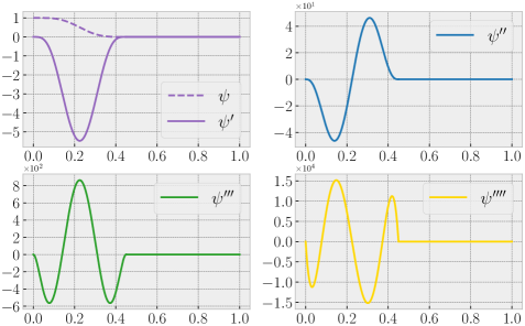
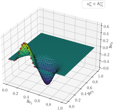
For our numerical experiments, we choose a setup from [43, Sec. 7], [18, §6], or [2, Sec. 5.1]. More precisely, let , , (cf. Figure 1(left)), i.e., , and . Then, we compute such that the primal solution , in polar coordinates centered at , i.e., for every , setting
for every , is defined by
Here, (cf. Figure 1(right)) is the zero extension of a ninth-order spline with respect to the single element partition of which satisfies for all , for all , and
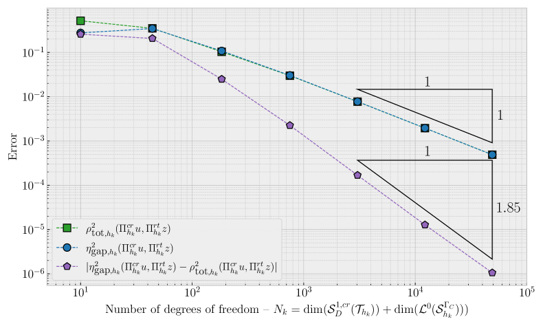
In this example, we have that , so that Theorem 6.6(ii) suggests an experimental convergence rate of about , where , , for the discrete primal-dual total errors (cf. (6.4)), which are equal to the discrete primal-dual gap estimators (cf. (6.1)), i.e., we expect (cf. Theorem 6.6(i))
An initial triangulation , , is constructed by subdividing the unit square along its diagonal from to into two triangles. Refined triangulations , , where for all , are obtained by applying the red-refinement routine (cf. [44]).
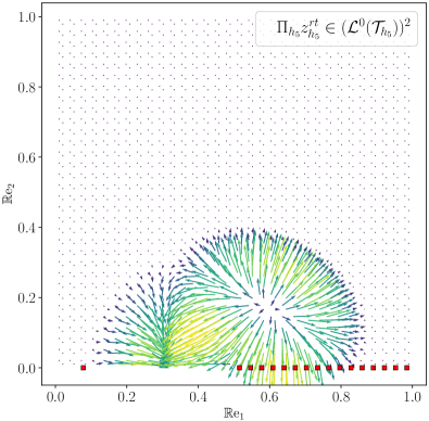
For the resulting series of triangulations , , we apply the primal-dual active set strategy (cf. Algorithm 7.1) to compute the discrete primal solution , , the discrete Lagrange multiplier , , and, subsequently, resorting to (5.17), the discrete dual solution , . Then, we compute the error quantities
| (7.4) |
For determining the convergence rates, the experimental order of convergence (EOC), i.e.,
where, for every , we denote by , either , , or , respectively, is recorded.
In Figure 3, we report the expected optimal convergence rate of , , i.e., an error decay of order , . In addition, we observe that the a priori error identity in Theorem 6.6(i) is asymptotically satisfied. More precisely, for the error between the discrete primal-dual total error (cf. (6.4)) and the discrete primal-dual gap estimator (cf. (6.1)), we report a convergence rate of about , , i.e., an error decay of order , , which is the quadrature error involved in the computation of the quasi-interpolants , , and , .
Numerical experiments concerning a posteriori error analysis
In this subsection, we review the theoretical findings of Section 4.
More precisely, we employ the local refinement indicators , , where
induced by the primal-dual gap estimator (cf. (4.1)), for every , , and , defined by
| (7.5) |
in an adaptive mesh-refinement scheme. The definition of the local refinement indicators (cf. (7.5)) is motivated by the representation of the primal-dual gap estimator (cf. (4.1)) in Lemma 4.1.
The numerical experiments are based on the following adaptive algorithm:
Algorithm 7.3 (AFEM).
Let , , and an initial triangulation of . Then, for every :
- (’Solve’)
-
Compute the discrete primal solution and the discrete dual solution .
Post-process and to obtain a conforming approximations and of the primal solution and the dual solution , respectively;
- (’Estimate’)
-
Compute the resulting local refinement primal-dual indicators . If , then STOP; otherwise, continue with step (’Mark’);
- (’Mark’)
-
Choose a minimal (in terms of cardinality) subset such that
- (’Refine’)
-
Perform a conforming refinement of to obtain such that each element is ‘refined’ in . Increase and continue with step (’Solve’).
Remark 7.4 (Implementation details).
- (i)
- (ii)
- (iii)
-
If , i.e., , then as an admissible approximation in step (’Solve’), we employ a contact boundary modified node-averaging quasi-interpolant, i.e.,
where denotes the shape basis of and, for every , we denote by the set of elements containing ;
- (iv)
-
By the primal-dual gap identity (cf. Theorem 4.5), the stopping criterion in step (’Estimate’) guarantees accuracy of and in terms of the primal-dual total error (cf. (4.4) with Lemma 6.3), i.e., in step (’Estimate’).
- (i)
-
If not otherwise specified, we employ the parameter in step (’Mark’).
- (ii)
- (iii)
Example with unknown primal and dual solution
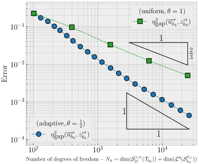
In this example, let , , (cf. Figure 4(left)), i.e., , , , and with for all . In this case, the primal solution is not known and since the Dirichlet part and the Neumann part touch in with interior angle (cf. Figure 4(left)), it cannot be expected to satisfy , so that uniform mesh refinement is expected to yield a reduced error decay rate compared to the quasi-optimal linear error decay rate.
Algorithm 7.3 refines the mesh towards the contact set and (cf. Figure 5), where we expect a singularity. In Figure 4(right), one finds that uniform mesh refinement (i.e., in Algorithm 7.3) yields the reduced convergence rate , , while adaptive mesh refinement (i.e., in Algorithm 7.3) yields the optimal convergence rate , .

Appendix A Appendix
In this appendix, we prove a lifting lemma that for a given element-wise constant vector field, a given element-wise constant function, and a given side-wise constant function defined on Neumann sides, jointly satisfying a compatibility condition, provides a Raviart–Thomas vector field whose (local) -projection coincides with the element-wise constant vector field, whose divergence coincides with the element-wise constant function, and whose normal traces coincide with the side-wise constant function on Neumann sides.
Lemma A.1 (lifting).
Let , , and be such that for every with a.e. on , there holds the compatibility condition
| (A.1) |
Then, the vector field defined by
| (A.2) |
satisfies and
| (A.3) | |||||
| (A.4) | |||||
| (A.5) |
Proof.
From the definition (A.2), it follows directly that (A.3) is satisfied. Since, due to , is surjective, there exists such that a.e. in . Then, using the discrete integration-by-parts formula (2.11) and (A.1), for every with a.e. on , we find that
| (A.6) |
Using (A.3) in (A.6), for every with a.e. on , we arrive at
| (A.7) |
On the other hand, due to in for all , we have that . By (A.7) and the discrete Helmholtz–Weyl decomposition (cf. [5, Sec. 2.4]), we conclude that
and, thus, with (A.4). In addition, for every with a.e. on , the discrete integration-by-parts formula (2.11) and (A.1) yield that
| (A.8) |
Thus, choosing for all in (A.8) and exploiting that , for every , we find that (A.5) is satisfied. ∎
References
- [1] T. Apel and S. Nicaise, Regularity of the solution of the scalar Signorini problem in polygonal domains, Result. Math. 75 no. 2 (2020), 15 (English), Id/No 75. doi:10.1007/s00025-020-01202-7.
- [2] B. S. Ashby and T. Pryer, Duality based error control for the signorini problem, 2024.
- [3] S. Bartels, Numerical methods for nonlinear partial differential equations, Springer Ser. Comput. Math. 47, Cham: Springer, 2015 (English). doi:10.1007/978-3-319-13797-1_1.
- [4] S. Bartels and A. Kaltenbach, Explicit and efficient error estimation for convex minimization problems, Math. Comput. 92 no. 343 (2023), 2247–2279 (English). doi:10.1090/mcom/3821.
- [5] S. Bartels and Z. Wang, Orthogonality relations of Crouzeix-Raviart and Raviart-Thomas finite element spaces, Numer. Math. 148 no. 1 (2021), 127–139 (English). doi:10.1007/s00211-021-01199-3.
- [6] J. Behrndt, F. Gesztesy, and M. Mitrea, Sharp boundary trace theory and schrödinger operators on bounded lipschitz domains, 2022.
- [7] F. Ben Belgacem, Numerical simulation of some variational inequalities arisen from unilateral contact problems by the finite element methods, SIAM J. Numer. Anal. 37 no. 4 (2000), 1198–1216. doi:10.1137/S0036142998347966.
- [8] F. Ben Belgacem and Y. Renard, Hybrid finite element methods for the Signorini problem, Math. Comp. 72 no. 243 (2003), 1117–1145. doi:10.1090/S0025-5718-03-01490-X.
- [9] F. Ben Belgacem, C. Bernardi, A. Blouza, and M. Vohralík, A finite element discretization of the contact between two membranes, M2AN Math. Model. Numer. Anal. 43 no. 1 (2009), 33–52. doi:10.1051/m2an/2008041.
- [10] F. Ben Belgacem, C. Bernardi, A. Blouza, and M. Vohralík, On the unilateral contact between membranes. Part 2: a posteriori analysis and numerical experiments, IMA J. Numer. Anal. 32 no. 3 (2012), 1147–1172. doi:10.1093/imanum/drr003.
- [11] F. Ben Belgacem and S. C. Brenner, Some nonstandard finite element estimates with applications to 3D Poisson and Signorini problems, Electron. Trans. Numer. Anal. 12 (2001), 134–148.
- [12] F. Ben Belgacem, P. Hild, and P. Laborde, Approximation of the unilateral contact problem by the mortar finite element method, C. R. Acad. Sci. Paris Sér. I Math. 324 no. 1 (1997), 123–127. doi:10.1016/S0764-4442(97)80115-2.
- [13] C. Carstensen, An adaptive mesh-refining algorithm allowing for an stable projection onto Courant finite element spaces, Constr. Approx. 20 no. 4 (2004), 549–564 (English). doi:10.1007/s00365-003-0550-5.
- [14] A. Chambolle and T. Pock, Crouzeix-Raviart approximation of the total variation on simplicial meshes, J. Math. Imaging Vis. 62 no. 6-7 (2020), 872–899 (English). doi:10.1007/s10851-019-00939-3.
- [15] F. Chouly and P. Hild, A Nitsche-based method for unilateral contact problems: numerical analysis, SIAM J. Numer. Anal. 51 no. 2 (2013), 1295–1307. doi:10.1137/12088344X.
- [16] F. Chouly and P. Hild, On convergence of the penalty method for unilateral contact problems, Appl. Numer. Math. 65 (2013), 27–40. doi:10.1016/j.apnum.2012.10.003.
- [17] F. Chouly, P. Hild, and Y. Renard, Symmetric and non-symmetric variants of Nitsche’s method for contact problems in elasticity: theory and numerical experiments, Math. Comp. 84 no. 293 (2015), 1089–1112. doi:10.1090/S0025-5718-2014-02913-X.
- [18] C. Christof and C. Haubner, Finite element error estimates in non-energy norms for the two-dimensional scalar Signorini problem, Numer. Math. 145 no. 3 (2020), 513–551 (English). doi:10.1007/s00211-020-01117-z.
- [19] M. Crouzeix and P.-A. Raviart, Conforming and nonconforming finite element methods for solving the stationary Stokes equations. I, Rev. Franc. Automat. Inform. Rech. Operat., R 7 no. 3 (1974), 33–76 (English). doi:10.1051/m2an/197307R300331.
- [20] L. Diening, P. Harjulehto, P. Hästö, and M. Růžička, Lebesgue and Sobolev spaces with variable exponents, Lect. Notes Math. 2017, Berlin: Springer, 2011 (English). doi:10.1007/978-3-642-18363-8.
- [21] W. Dörfler, A convergent adaptive algorithm for Poisson’s equation, SIAM J. Numer. Anal. 33 no. 3 (1996), 1106–1124 (English). doi:10.1137/0733054.
- [22] G. Drouet and P. Hild, Optimal convergence for discrete variational inequalities modelling Signorini contact in 2D and 3D without additional assumptions on the unknown contact set, SIAM J. Numer. Anal. 53 no. 3 (2015), 1488–1507. doi:10.1137/140980697.
- [23] I. Ekeland and R. Témam, Convex analysis and variational problems., unabridged, corrected republication of the 1976 English original ed., Class. Appl. Math. 28, Philadelphia, PA: Society for Industrial and Applied Mathematics, 1999 (English).
- [24] A. Ern and J.-L. Guermond, Finite elements I. Approximation and interpolation, Texts Appl. Math. 72, Cham: Springer, 2020 (English). doi:10.1007/978-3-030-56341-7.
- [25] A. Ern and J.-L. Guermond, Finite elements II. Galerkin approximation, elliptic and mixed PDEs, Texts Appl. Math. 73, Cham: Springer, 2021 (English). doi:10.1007/978-3-030-56923-5.
- [26] G. Fichera, Problemi elastostatici con vincoli unilaterali: Il problema di Signorini con ambigue condizioni al contorno, Atti Accad. Naz. Lincei, Mem., Cl. Sci. Fis. Mat. Nat., VIII. Ser., Sez. I 7 (1964), 91–140 (Italian).
- [27] L. G. Grisvard, Pierre, Problèmes aux limites unilatéraux dans des domaines non réguliers, Publications mathématiques et informatique de Rennes no. 1 (1976), 1–26 (fre).
- [28] P. Grisvard, Elliptic problems in nonsmooth domains, Monogr. Stud. Math. 24, Pitman, Boston, MA, 1985 (English).
- [29] P. Hild and S. Nicaise, A posteriori error estimations of residual type for Signorini’s problem, Numer. Math. 101 no. 3 (2005), 523–549. doi:10.1007/s00211-005-0630-5.
- [30] P. Hild and Y. Renard, An improved a priori error analysis for finite element approximations of Signorini’s problem, SIAM J. Numer. Anal. 50 no. 5 (2012), 2400–2419. doi:10.1137/110857593.
- [31] D. Hua and L. Wang, The nonconforming finite element method for Signorini problem, J. Comput. Math. 25 no. 1 (2007), 67–80 (English).
- [32] S. Hüeber and B. I. Wohlmuth, An optimal a priori error estimate for nonlinear multibody contact problems, SIAM J. Numer. Anal. 43 no. 1 (2005), 156–173. doi:10.1137/S0036142903436678.
- [33] J. D. Hunter, Matplotlib: A 2d graphics environment, Computing in Science & Engineering 9 no. 3 (2007), 90–95. doi:10.1109/MCSE.2007.55.
- [34] R. Krause, A. Veeser, and M. Walloth, An efficient and reliable residual-type a posteriori error estimator for the Signorini problem, Numer. Math. 130 no. 1 (2015), 151–197. doi:10.1007/s00211-014-0655-8.
- [35] M. Li, D. Hua, and H. Lian, On nonconforming finite element aproximation for the Signorini problem, Electron. Res. Arch. 29 no. 2 (2021), 2029–2045 (English). doi:10.3934/era.2020103.
- [36] A. Logg, K.-A. Mardal, and G. Wells (eds.), Automated solution of differential equations by the finite element method. The FEniCS book, Lect. Notes Comput. Sci. Eng. 84, Berlin: Springer, 2012 (English). doi:10.1007/978-3-642-23099-8.
- [37] M. Moussaoui and K. Khodja, Regularity of solutions for a mixed Dirichlet-Signorini problem in a plane polygonal domain, Commun. Partial Differ. Equations 17 no. 5-6 (1992), 805–826 (French). doi:10.1080/03605309208820864.
- [38] P. A. Raviart and J. M. Thomas, A mixed finite element method for 2nd order elliptic problems, Math. Aspects Finite Elem. Meth., Proc. Conf. Rome 1975, Lect. Notes Math. 606, 292-315 (1977)., 1977.
- [39] S. Repin and J. Valdman, Error identities for variational problems with obstacles, ZAMM, Z. Angew. Math. Mech. 98 no. 4 (2018), 635–658 (English). doi:10.1002/zamm.201700105.
- [40] A. Schröder, Mixed finite element methods of higher-order for model contact problems, SIAM J. Numer. Anal. 49 no. 6 (2011), 2323–2339. doi:10.1137/090770072.
- [41] A. Signorini, Questioni di elasticità non linearizzata e semilinearizzata, Rend. Mat. Appl., V. Ser. 18 (1959), 95–139 (Italian).
- [42] W. Spann, On the boundary element method for the Signorini problem of the Laplacian, Numer. Math. 65 no. 3 (1993), 337–356 (English). doi:10.1007/BF01385756.
- [43] O. Steinbach, B. Wohlmuth, and L. Wunderlich, Trace and flux a priori error estimates in finite-element approximations of Signorini-type problems., IMA J. Numer. Anal. 36 no. 3 (2016), 1072–1095 (English). doi:10.1093/imanum/drv039.
- [44] R. Verfürth, A posteriori error estimation techniques for finite element methods, Numer. Math. Sci. Comput., Oxford: Oxford University Press, 2013 (English).
- [45] L. Wang, Nonconforming finite element approximations to the unilateral problem, J. Comput. Math. 17 no. 1 (1999), 15–24 (English).
- [46] A. Weiss and B. I. Wohlmuth, A posteriori error estimator and error control for contact problems, Math. Comp. 78 no. 267 (2009), 1237–1267. doi:10.1090/S0025-5718-09-02235-2.