SVD Entanglement Entropy of Chiral Dirac Oscillators

Abstract

We discuss the SVD entanglement entropy, which has recently come up as a successor to the pseudo entropy. This paper is a first-of-its-kind application of SVD entanglement entropy to a system of chiral Dirac oscillators which prove to be natural to study the SVD formalism because the two chiral oscillator ground states can be taken as the pre-selected and post-selected states. We argue how this alternative for entanglement entropy is better and more intuitive than the von Neumann one to study quantum phase transition. We also provide as an illustrative example, a new generalized proof of the SVD entanglement entropy being $\log 2$ for a pair of Bell states that differ from each other by relative phases.

INTRODUCTION
Entanglement entropy is a measure of the quantum correlation or entanglement between two subsystems in a quantum system. It has become an important parameter in studying the quantum properties of any emergent quantum system. Entanglement entropy is usually computed by the definition of entropy given by von Neumann [1] and is called the von Neumann entanglement entropy. Here we consider a single state and compute the entanglement entropy which is a measure of quantum correlations among the degrees of freedom for the given state. Recently however a new way has been devised to calculate entanglement entropy using the SVD (Singular Value Decomposition) entanglement entropy proposed in [2]. In this we take two states and form a density matrix from these states rather than taking the same state, these states are called pre-selection and post-selection states, and then the entanglement entropy gives the measure of quantum correlations among the degrees of freedom for the post-selection and pre-selection states. It is observed that this result of SVD entanglement entropy comes out close to the usual von Neumann entanglement entropy. After the original work [2] some papers citing SVD entropy have also appeared [3, 4, 5, 6, 7, 8, 9, 10, 11, 12, 13] where it has been considered as a further generalization of the pseudo entropy [14].

Here we concern ourselves with the entanglement entropy related to the states of the Dirac oscillator which is a relativistic fermionic harmonic oscillator in the presence of a constant magnetic field. These oscillators were first studied in [15, 16] and prove to be a very interesting system to study in quantum optics and condensed matter physics. In recent decades a lot of work has been put into the theoretical [17, 18] as well as experimental advancement [19] of this in terms of its thermal properties [20], further generalizations [21, 22] and its applications to cosmology and gravitational systems [23, 24, 25] have also come up. In work done by Bermudez et al. in [26], it was shown that these Dirac oscillators in the presence of a constant magnetic field exhibit a quantum phase transition. This study calculated the analytical expression for order parameter, and canonical quantum fluctuations for the quantum phase transition, furthermore, entanglement properties between the degrees of freedom in the relativistic ground state were also studied. The entanglement entropy turns out to be divergent at the point of phase transition which is seen as a common feature of quantum phase transition [27, 28, 29, 30].

In this work, we have shown how SVD entanglement entropy is used to calculate the entanglement entropy for a system exhibiting chiral behavior. Our results show that the behavior of SVD entanglement entropy is similar to [26] but the physical interpretation is more intuitive than the von Neumann entanglement entropy. The SVD entanglement entropy is the entanglement across the quantum phase transition of the degrees of freedom of the ground states. In both cases, the value of entanglement entropy is divergent at the critical point indicative of a quantum phase transition [2, 30].

As a prelude to the study of chiral Dirac oscillators, we provide as an illustrative example, a new generalized proof of the SVD entanglement entropy being $\log 2$ for a pair of Bell states that differ from each other by relative phases. This is a generalization of a result given in [2] where they have considered a specific example of a Bell state and the same Bell state but with a relative phase as pre-selection and post-selection states respectively. This work is also a first-of-its-kind example of the application of SVD entanglement entropy in a quantum optical system. All the other studies are based on holographic CFTs as cited above.

The organization of this paper is as follows. In the first section, we introduce the SVD entanglement entropy and its basic properties, brief the work done in [2] along with the generalized example for Bell states. In the second section, we introduce the formalism related to the chiral Dirac oscillator. Non-relativistic oscillators and chirality have been studied in a fundamental and field-theoretic manner by [31, 32, 33] its connection to material science and topological Chern-Simons gauge theory has been pointed out in [34, 35]. In the third section, we introduce our main result and compare it with the old result for entanglement entropy. Conclusions are given in the last section.

1 SVD ENTANGLEMENT ENTROPY

There have been numerous ways that try to incorporate a post-selection and pre-selection state into the calculation of entanglement entropy, as it is a useful formalism for treating problems in quantum gravity, black hole information paradox, condensed matter physics [36, 37, 14, 38, 39, 40, 41, 42, 43] and quantum information theory [44, 45, 46, 47]. The aim of this section is to introduce this new definition of entropy as elaborated in [2]. This definition is the general definition for entanglement entropy which tries to solve the problem of considering pre-selection and post-selection states.

We are already familiar with the von Neumann entropy for a bipartite system. If $\rho$ represents the density operator of the system then, the von Neumann entropy is given by,

$$S=-Tr(\rho\log\rho)$$

But this definition of entropy uses only a single state and that state may be entangled or not.

The SVD (single value decomposition) entanglement entropy uses two states a pre-selected state and a post-selected state to calculate the entanglement entropy. It is proposed to be a natural generalization of the von Neumann entanglement entropy.

Consider a Hilbert space that is decomposed into two Hilbert spaces $\mathcal{H}=\mathcal{H}_{A}\otimes\mathcal{H}_{B}$ if we take $|\psi_{1}\rangle$ as the pre-selected state and $|\psi_{2}\rangle$ as the post-selected state, then we can define the reduced transition matrix[2],

$$\tau^{1|2}:=\frac{|\psi_{1}\rangle\langle\psi_{2}|}{\langle\psi_{1}|\psi_{2}\rangle}$$ (1)

whereas the unnormalized version is,

$$\tau^{1|2}=|\psi_{1}\rangle\langle\psi_{2}|$$

Now if we take the partial trace,

$$\tau^{1|2}_{A}=Tr_{B}[\tau^{1|2}]$$

Using this we define,

$$\rho^{1|2}_{A}:=\frac{\sqrt{(\tau^{1|2}_{A})^{\dagger}(\tau^{1|2}_{A})}}{Tr\left[\sqrt{(\tau^{1|2}_{A})^{\dagger}(\tau^{1|2}_{A})}\right]}$$ (2)

This operator is a density operator. Using this we define the SVD entropy as,

$$S_{SVD}(\tau^{1|2}_{A}):=-Tr[\rho^{1|2}_{A}\log\rho^{1|2}_{A}]$$ (3)

Hence, the functional form of SVD and von Neumann entanglement entropy is similar.[2]
Now, we try to summarise the general definition and physical interpretation (in the context of information theory) as given in [2].
General Definition: Given a space $\mathbb{M}_{m}$ of $m\times m$ matrices. Then $S_{SVD}$ is defined by,

$$S_{SVD}:\mathbb{M}_{m}\longrightarrow\left[0,\infty\right)$$

$$S_{SVD}(A)=S_{vN}\left(\frac{|A|}{||A||_{1}}\right)=-\sum^{m}_{i=1}\frac{\sigma_{i}}{||A||_{1}}\log\left(\frac{\sigma_{i}}{||A||_{1}}\right)$$

where $|A|:=\sqrt{A^{\dagger}A}$ and, $||A||_{1}:=Tr|A|=\sum^{m}_{i=1}\sigma_{i}$ ($\sigma_{i}$ are eigenvalues of $|A|$). Also note if $A=0$ then $S_{SVD}=0$.[2]
Physical Interpretation: von Neumann entropy coincides with the average number of Bell pairs that can be distilled from a given bipartite state via local operations and classical communication[48, 1]. This result can also be proved for SVD entropy.[2]

We can also diagonalize the reduced transition matrix,

$$\tau^{1|2}=U\cdot\Lambda\cdot V^{\dagger}$$

where $U$ and $V$ are unitary matrices, and $\Lambda$ is the diagonal matrix such that $\Lambda=diag(\lambda_{1},\ldots,\lambda_{d_{A}})$ and $\lambda_{i}\geq 0,\forall i\in\{1,\ldots,d_{A}\}$. Then we can define the normalized eigenvalues as:

$$\hat{\lambda}_{i}=\frac{\lambda_{i}}{\sum\lambda_{i}}$$

Clearly, $\hat{\lambda}_{i}$ are eigenvalues of $\rho^{1|2}_{A}$, then we have:

$$S_{SVD}=-\sum^{d_{A}}_{i}\hat{\lambda}_{i}\log\hat{\lambda}_{i}$$

These are all parts of standard results and definitions done in [2].

1.1 General Result for the Bell States

Now, we make a general statement about the SVD entropy of the Bell states. In [2] two states belonging to a bipartite system of bell states ($\mathcal{H}_{A}\otimes\mathcal{H}_{B}$) have been considered as:

$$\begin{split}|\psi_{1}\rangle&=\frac{1}{\sqrt{2}}(|00\rangle+|11\rangle)\\ |\psi_{2}\rangle&=\frac{1}{\sqrt{2}}(|00\rangle+\phi|11\rangle)\end{split}$$ (4)

where $\phi\in\mathbf{C}$, $|\phi|=1$, and $|\psi_{1}\rangle$ and $|\psi_{2}\rangle$ are the pre-selected and post-selected states respectively.
Now we consider the following generalized states belonging to a bipartite system of bell states ($\mathcal{H}_{A}\otimes\mathcal{H}_{B}$).

$$\begin{split}|\psi_{1}\rangle&=a|\alpha\beta\rangle+b|\gamma\delta\rangle,\\ |\psi_{2}\rangle&=c|\tilde{\alpha}\tilde{\beta}\rangle+d|\tilde{\gamma}\tilde{\delta}\rangle\end{split}$$ (5)

where $\alpha,\beta,\gamma,\delta,\tilde{\alpha},\tilde{\beta},\tilde{\gamma}$, and $\tilde{\delta}\in\{0,1\}$ and $a,b,c,d$ $\in\mathbf{C}$, $|a|,|b|,|c|,|d|=1$. The transition matrix is given by,

$$\tau^{1|2}=\frac{|\psi_{1}\rangle\langle\psi_{2}|}{\langle\psi_{1}|\psi_{2}\rangle}$$

$$\tau^{1|2}=\frac{ac^{*}|\alpha\beta\rangle\langle\tilde{\alpha}\tilde{\beta}|+ad^{*}|\alpha\beta\rangle\langle\tilde{\gamma}\tilde{\delta}|+ba^{*}|\gamma\delta\rangle\langle\tilde{\alpha}\tilde{\beta}|+bd^{*}|\gamma\delta\rangle\langle\tilde{\gamma}\tilde{\delta}|}{a^{*}c\langle\alpha\beta|\tilde{\alpha}\tilde{\beta}\rangle+a^{*}d\langle\alpha\beta|\tilde{\gamma}\tilde{\delta}\rangle+b^{*}c\langle\gamma\delta|\tilde{\alpha}\tilde{\beta}\rangle+b^{*}d\langle\gamma\delta|\tilde{\gamma}\tilde{\delta}\rangle}$$

The reduced transition matrix is,

$$\tau^{1|2}_{A}=Tr_{B}(\tau^{1|2})$$

$$\tau^{1|2}_{A}=\frac{ac^{*}|\alpha\rangle\langle\tilde{\alpha}|(\langle\beta|\tilde{\beta}\rangle)+ad^{*}|\alpha\rangle\langle\tilde{\gamma}|(\langle\beta|\tilde{\delta}\rangle)+bc^{*}|\gamma\rangle\langle\tilde{\alpha}|(\langle\delta|\tilde{\beta}\rangle)+bd^{*}|\gamma\rangle\langle\tilde{\gamma}|(\langle\delta|\tilde{\delta}\rangle)}{a^{*}c\langle\alpha\beta|\tilde{\alpha}\tilde{\beta}\rangle+a^{*}d\langle\alpha\beta|\tilde{\gamma}\tilde{\delta}\rangle+b^{*}c\langle\gamma\delta|\tilde{\alpha}\tilde{\beta}\rangle+b^{*}d\langle\gamma\delta|\tilde{\gamma}\tilde{\delta}\rangle}$$

Since these are Bell states:

• Case I: If without loss of generality we assume that $\alpha=\beta=0$ $\implies$ $\gamma$, $\delta=1$ (Bell states).

  $$\tau^{1|2}_{A}=\frac{ac^{*}|0\rangle\langle\tilde{\alpha}|(\langle 0|\tilde{\beta}\rangle)+ad^{*}|0\rangle\langle\tilde{\gamma}|(\langle 0|\tilde{\delta}\rangle)+bc^{*}|1\rangle\langle\tilde{\alpha}|(\langle 1|\tilde{\beta}\rangle)+bd^{*}|1\rangle\langle\tilde{\gamma}|(\langle 1|\tilde{\delta}\rangle)}{a^{*}c\langle 00|\tilde{\alpha}\tilde{\beta}\rangle+a^{*}d\langle 00|\tilde{\gamma}\tilde{\delta}\rangle+b^{*}c\langle 11|\tilde{\alpha}\tilde{\beta}\rangle+b^{*}d\langle 11|\tilde{\gamma}\tilde{\delta}\rangle}$$

  Also for the denominator to be non-zero $\tilde{\alpha}=\tilde{\beta}$ and $\tilde{\gamma}=\tilde{\delta}$. Since we are working with Bell states $\implies$ $\tilde{\alpha}\neq\tilde{\gamma}$.
  Again, without loss of generality assume that, $\tilde{\gamma}=0$ and $\tilde{\alpha}=1$, then,

  $$\tau^{1|2}_{A}=\frac{\left[ad^{*}|0\rangle\langle 0|+bc^{*}|1\rangle\langle 1|\right]}{(a^{*}d+b^{*}c)}$$ (6)

  If we had used the complimentary values i.e. $\tilde{\gamma}=1$ and $\tilde{\alpha}=0$, then,

  $$\tau^{1|2}_{A}=\frac{\left[ac^{*}|0\rangle\langle 0|+bd^{*}|1\rangle\langle 1|\right]}{(a^{*}c+b^{*}d)}$$ (7)

• Case II: If $\alpha=\delta$ then $\beta=\gamma$, $\alpha\neq\beta$ and $\gamma\neq\delta$, so without loss of generality if we assume that $\alpha=0$ then $\beta=1$, $\gamma=1$, and $\delta=0$.

  $$\tau^{1|2}_{A}=\frac{ac^{*}|0\rangle\langle\tilde{\alpha}|(\langle 1|\tilde{\beta}\rangle)+ad^{*}|0\rangle\langle\tilde{\gamma}|(\langle 1|\tilde{\delta}\rangle)+bc^{*}|1\rangle\langle\tilde{\alpha}|(\langle 0|\tilde{\beta}\rangle)+bd^{*}|1\rangle\langle\tilde{\gamma}|(\langle 0|\tilde{\delta}\rangle)}{a^{*}c\langle 01|\tilde{\alpha}\tilde{\beta}\rangle+a^{*}d\langle 01|\tilde{\gamma}\tilde{\delta}\rangle+b^{*}c\langle 10|\tilde{\alpha}\tilde{\beta}\rangle+b^{*}d\langle 10|\tilde{\gamma}\tilde{\delta}\rangle}$$

  Also for the denominator to be non-zero $\tilde{\alpha}\neq\tilde{\beta}$ and $\tilde{\gamma}\neq\tilde{\delta}$. Since we are working with Bell states $\implies$ $\tilde{\alpha}=\tilde{\delta}$ and $\tilde{\beta}=\tilde{\gamma}$.
  Again, without loss of generality assume that, $\tilde{\alpha}=1$ and $\tilde{\beta}=0$, then,

  $$\tau^{1|2}_{A}=\frac{\left[ad^{*}|0\rangle\langle 0|+bc^{*}|1\rangle\langle 1|\right]}{(a^{*}d+b^{*}c)}$$ (8)

  If we had assumed the complimentary values i.e. $\tilde{\alpha}=0$ and $\tilde{\beta}=0$, then,

  $$\tau^{1|2}_{A}=\frac{\left[ac^{*}|0\rangle\langle 0|+bd^{*}|1\rangle\langle 1|\right]}{(a^{*}c+b^{*}d)}$$ (9)

Now, we evaluate the density matrix from the reduced transition matrix.

$$\rho^{1|2}_{A}=\frac{\sqrt{(\tau^{1|2}_{A})^{\dagger}\tau^{1|2}_{A}}}{Tr\left(\sqrt{(\tau^{1|2}_{A})^{\dagger}\tau^{1|2}_{A}}\right)}$$

$$\rho^{1|2}_{A}=\frac{\sqrt{\frac{|ad|^{2}|0\rangle\langle 0|+|bc|^{2}|1\rangle\langle 1|}{(a^{*}d+bc^{*})(ad^{*}+b^{*}c)}}}{Tr\left(\sqrt{\frac{|ad|^{2}|0\rangle\langle 0|+|bc|^{2}|1\rangle\langle 1|}{(a^{*}d+bc^{*})(ad^{*}+b^{*}c)}}\right)}$$

$$\rho^{1|2}_{A}=\frac{|0\rangle\langle 0|+|1\rangle\langle 1|}{2}$$

$$S_{SVD}=-Tr\left(\rho^{1|2}_{A}\log\rho^{1|2}_{A}\right)=\log 2$$ (10)

Thus the entropy for Bell states is $\log 2$ which is equal to the value of von Neumann entropy for Bell states. This result confirms the validity of SVD entanglement entropy as a generalization of the usual von Neumann entanglement entropy for two different states. In [2] the $\log 2$ result was obtained for the particular choice (4).

2 CHIRAL DIRAC OSCILLATORS

In the previous example, introducing by hand a phase among the Bell states, the pre-selected and post-selected states were defined. Chiral Dirac oscillators, on the other hand, provide a natural setting for obtaining these states by considering the opposite chiralities. The Dirac equation gives the Dirac oscillator in its usual framework [15, 16]:

$$i\hbar\frac{\partial|\psi\rangle}{\partial t}=[c\boldsymbol{\alpha}(\textbf{p}-im\beta\omega\textbf{r}+e\textbf{A})+\beta mc^{2}]|\psi\rangle$$ (11)

where m is the relativistic mass of the fermion, $-e$ is the electric charge, $|\psi\rangle$ stands for the Dirac four-component spinor, r and p represent position and momentum operators, $\omega$ is the Dirac oscillator frequency, $c$ is the speed of light and $\beta:=diag(\mathbf{I},-\mathbf{I})$, $\alpha_{j}:=off-diag(\sigma_{j},\sigma_{j})$ are the Dirac matrices related to the usual Pauli matrices. This relativistic oscillator involves two phonon modes. Now, if we introduce the magnetic field by minimal coupling $\textbf{p}\longrightarrow\textbf{p}+e\textbf{A}$ where A is the vector potential related to the magnetic field. In the two-dimensional setup, the Dirac matrices become the Pauli matrices [26, 49], then (11) becomes:

$$i\hbar\frac{\partial|\psi\rangle}{\partial t}=\left[c\sum^{2}_{j=1}\sigma_{j}(p_{j}-im\beta\sigma_{z}x_{j}+eA_{j})+\sigma_{z}mc^{2}\right]|\psi\rangle$$ (12)

where $|\psi\rangle$ is a two-component spinor that mixes spin-up and spin-down with positive and negative energies. The non-minimal coupling of Dirac oscillator ($\textbf{p}-im\beta\omega\textbf{r}$) and the minimal coupling of the magnetic field endows the particle with intrinsic left-handed and right-handed chirality respectively [26, 50, 51].

2.1 Mapping onto a Simultaneous JC-AJC Hamiltonian

The above Hamiltonian in (11) can be mapped onto a simultaneous Jaynes Cummings and Anti-Jaynes-Cummings Hamiltonian[52]. Here we enlist the final results of this mapping and the associated energy spectrum and ground states (next section) obtained in [26, 51] to proceed with the discussion of entropy in the third section.

$$H=\delta\sigma_{z}-H^{\circlearrowright}_{JC}(g_{r})+H^{\circlearrowleft}_{AJC}(g_{l})$$ (13)

where $\delta=mc^{2}$ stands for the detuning parameter proportional to the rest mass energy, $H^{\circlearrowright}_{JC}(g_{r})$ represents a right-handed Jaynes-Cummings Hamiltonian

$$H^{\circlearrowright}_{JC}(g_{r})=g_{r}\sigma^{+}\tilde{a}_{r}+g_{r}^{*}\sigma^{-}\tilde{a}_{r}^{\dagger}$$

with $g_{r}:=imc^{2}\sqrt{2\tilde{\xi}}$ as the interaction coupling strength. Analogously, the term $H^{\circlearrowleft}_{AJC}(g_{l})$ stands for a left-handed Anti-Jaynes-Cummings interaction

$$H^{\circlearrowleft}_{AJC}(g_{l})=g_{l}\sigma^{+}a_{l}^{\dagger}+g_{l}^{*}\sigma^{-}a_{l}$$

with a similar coupling strength $g_{l}:=imc^{2}\sqrt{2{\xi}}$
Now we introduce the circular annihilation-creation operators ($\tilde{a}_{r}\>\text{and}\>a_{l}$) used in the above equations as defined in [26, 51]. Using the axial gauge ($A_{0}=0$) the magnetic field in the Dirac oscillator is defined as $\mathbf{B}=B\mathbf{e}_{z}$ with the vector potential $\mathbf{A}:=\frac{B}{2}\left[-y,x,0\right]$. We describe the dynamics by two frequencies, the Dirac oscillator frequency $\omega$ and the cyclotron frequency $\omega_{c}=eB/m$. Hence, the annihilation-creation operators are:

$$a_{i}=\frac{1}{\sqrt{2}}\left(\frac{1}{\triangle}r_{i}-i\frac{\triangle}{\hbar}p_{i}\right),\tilde{a}_{i}=\frac{1}{\sqrt{2}}\left(\frac{1}{\tilde{\triangle}}r_{i}-i\frac{\tilde{\triangle}}{\hbar}p_{i}\right)$$

where $\triangle:=\sqrt{\hbar/m\omega}$, $\tilde{\triangle}:=\sqrt{\hbar/m\tilde{\omega}}$ and $\tilde{\omega}=w_{c}/2$. The basic commutation relations are,

$$\begin{split}[a_{i},\tilde{a}_{j}]=\frac{1}{2}\left[\frac{\triangle}{\tilde{\triangle}}-\frac{\tilde{\triangle}}{\triangle}\right]\delta_{ij},\\ [a_{i},\tilde{a}_{j}^{\dagger}]=\frac{1}{2}\left[\frac{\triangle}{\tilde{\triangle}}+\frac{\tilde{\triangle}}{\triangle}\right]\delta_{ij}\end{split}$$ (14)

We have introduced $i=x,y$ to account for two possible directions for equations of motion. Also note that $\tilde{\xi}=\hbar\tilde{\omega}/mc^{2}$ and $\xi=\hbar\omega/mc^{2}$.
So the circular annihilation-creation operators for each frequency are:

$$\tilde{a}_{r}=\frac{1}{\sqrt{2}}(\tilde{a}_{x}-i\tilde{a}_{y}),\>\>\>\>\tilde{a}_{l}=\frac{1}{\sqrt{2}}(\tilde{a}_{x}+i\tilde{a}_{y}),\>\>\>\>a_{r}=\frac{1}{\sqrt{2}}(a_{x}-ia_{y}),\>\>\>\>a_{l}=\frac{1}{\sqrt{2}}(a_{x}+ia_{y})$$ (15)

2.2 Exact Solution: Energy Spectrum and Eigenstates

In this section, we summarise the results of a unitary transformation that converts the bi-chromatic Hamiltonian in (13) into a monochromatic JC(AJC) term that includes a bosonic degree of freedom with a certain chirality that depends upon external parameters $\xi>\tilde{\xi}(\xi<\tilde{\xi})$ [26, 51].

2.2.1 Left-Handed Regime $\tilde{\xi}<\xi$

Under the above conditions, the Hamiltonian given in (13) can be mapped onto a single-mode anti-Jaynes-Cummings Hamiltonian by using the unitary transformation:

$$U_{\alpha}:=e^{\alpha(a_{l}\tilde{a}_{r}-\tilde{a}_{r}^{\dagger}a_{l}^{\dagger})}$$ (16)

where the real parameter $\alpha$ depends on the relative strength of the oscillator and magnetic couplings:

$$\alpha:=\frac{1}{\lambda}\text{arctanh}\left(\frac{\lambda\sqrt{\tilde{\omega}}}{\sqrt{\omega}-\mu\sqrt{\tilde{\omega}}}\right)$$ (17)

with $\mu:=(\triangle/\tilde{\triangle}-\tilde{\triangle}/\triangle)/2$ and $\lambda:=\sqrt{\mu^{2}+1}$. Two Hermitian operators related through a unitary operator share a common spectrum, hence in the weak magnetic field regime:

$$E=\pm E_{n_{l}}=\pm mc^{2}\sqrt{1+2*\zeta_{l}(\xi,\tilde{\xi})(n_{l}+1)}$$ (18)

where $\zeta_{l}(\xi,\tilde{\xi}):=\xi-\tilde{\xi}-2\mu(\xi\tilde{\xi})^{1/2}$ is related to the initial relevant parameters and $n_{l}=0,1,...$ represents the number of left-handed quanta. This transformation can be immediately related to a two-mode squeezing operator in the context of quantum optics with squeezing parameter $z:=-\alpha\tilde{\mu}/2\in\mathbf{R}$ [53]. The action of such a squeezing operator (16) over left-handed chiral Fock states gives rise to SU(1,1) coherent states $|z,n_{l}\rangle:=U^{\dagger}_{\alpha}|n_{l}\rangle|vac\rangle_{r}$ [26, 54].

$$|z,n_{l}\rangle=\cosh^{-(n_{l}+1)}|z|\sum^{\infty}_{m=0}\sqrt{\frac{(m+n_{l})!}{n_{l}!m!}}(-1)^{m}\tanh^{m}|z||m+n_{l},m\rangle$$ (19)

For the fermionic ground state

$$E_{g}=mc^{2}$$ (20)

$$|g\rangle=|z,0\rangle|\chi_{\uparrow}\rangle=\frac{1}{\cosh|z|}\sum^{\infty}_{m=0}(-1)^{m}\tanh^{m}|z||m,m\rangle|\chi_{\uparrow}\rangle$$ (21)

and is interpreted as a spin-up squeezed vacuum state, where the squeezing parameter $z:=-\alpha\tilde{\mu}/2$ depends on the relative coupling strengths $\xi,\tilde{\xi}$.

2.2.2 Right-Handed Regime $\tilde{\xi}>\xi$

In this condition, we transform the Hamiltonian into a Jaynes-Cummings Hamiltonian by the unitary transformation.

$$U_{\tilde{\alpha}}:=e^{\tilde{\alpha}(a_{l}\tilde{a}_{r}-\tilde{a}_{l}^{\dagger}a_{l}^{\dagger})}$$ (22)

where the parameter $\tilde{\alpha}$ is,

$$\tilde{\alpha}=\frac{1}{\lambda}\text{arctanh}\left(\frac{\lambda\sqrt{\omega}}{\sqrt{\tilde{\omega}}+\mu\sqrt{\omega}}\right)$$

The energy spectrum becomes,

$$\tilde{E}=\pm\tilde{E}_{n_{r}}=\pm mc^{2}\sqrt{1+2\zeta_{r}(\xi,\tilde{\xi})(n_{r}+1)}$$ (23)

where $\zeta_{r}(\xi,\tilde{\xi}):=\tilde{\xi}-\xi+2\mu(\tilde{\xi}\xi)^{1/2}$ and $n_{r}=0,1,...,$ represents the number of right-handed quanta. In this case, the squeezing parameter becomes $\tilde{z}:=-\tilde{\alpha}\tilde{\mu}/2\in\mathcal{R}$ and the SU(1,1) coherent states $|\tilde{z},n_{r}\rangle:=U^{\dagger}_{\tilde{\alpha}}|vac\rangle_{l}|n_{r}\rangle$[26].

$$|\tilde{z},n_{r}\rangle=\cosh^{-(n_{r}+1)}|\tilde{z}|\sum^{\infty}_{\tilde{m}=0}\sqrt{\frac{(\tilde{m}+n_{r})!}{n_{r}!\tilde{m}!}}(-1)^{\tilde{m}}\tanh^{\tilde{m}}|\tilde{z}||\tilde{m}+n_{r},\tilde{m}\rangle$$ (24)

We also see how the fermionic ground state in this case differs from the left-handed regime one (21) as:

$$E_{\tilde{g}}=mc^{2}\sqrt{1+2\zeta_{r}}$$ (25)

$$|\tilde{g}\rangle=\tilde{C}_{0+}|\tilde{z},0\rangle|\chi_{\uparrow}\rangle-i\tilde{C}_{0-}|\tilde{z},1\rangle|\chi_{\downarrow}\rangle$$ (26)

where $\tilde{C}_{n_{r}\pm}:=[(\tilde{E}_{n_{r}}\pm mc^{2}).2\tilde{E}_{n_{r}}]^{1/2}$, and is interpreted as a spin-up squeezed vacuum state, where the squeezing parameter $\tilde{z}:=-\tilde{\alpha}\tilde{\mu}/2$ depends on the relative coupling strengths $\xi,\tilde{\xi}$.

2.2.3 Critical Regime $\tilde{\xi}=\xi$

In this regime, the magnetic field coupling cancels the effect of the Dirac string couple, hence we get a free relativistic fermionic particle [26]. The energy spectrum is given by:

$$E^{c}=\pm E^{c}_{\textbf{p}}=\pm\sqrt{m^{2}c^{4}+\textbf{p}^{2}c^{2}}$$ (27)

where $\textbf{p}=(p_{x},p_{y})$ stands for two dimensional fermion momentum. We can see that the energy is the usual free particle energy. The eigenstates are described as:

$$|\pm E^{c}_{\textbf{p}}\rangle=\sqrt{\frac{mc^{2}\pm E^{c}_{\textbf{p}}}{\pm 2E^{c}_{\textbf{p}}}}\left(|\chi_{\uparrow}\rangle+\frac{c(p_{x}+ip_{y})}{mc^{2}\pm E^{c}_{\textbf{p}}}|\chi_{\downarrow}\rangle\right)|\textbf{p}\rangle$$ (28)

where $\textbf{p}:=|p_{x},p_{y}\rangle$ are two-dimensional plane wave solutions.

A schematic showing a simplified version of the set-up is shown in Figure 1.
Using these results Bermudez et al. in [26] showed how the quantum phase transition occurs by plotting the energy spectrum as a function of relative coupling strength, studied the order parameter, the divergence of quantum fluctuations, and the entanglement entropy. The dependence of the magnetic field provides a control parameter to test the properties of the system such as chirality, squeezing, phonon statistics, and entanglement.

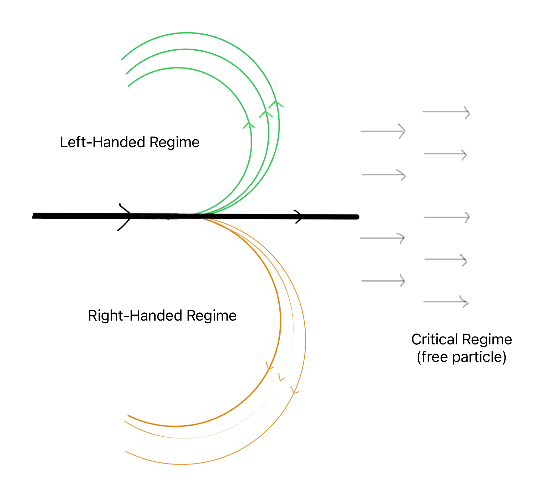
Figure 1: This cartoon represents the classical trajectory of a particle in a cyclotron. The various arcs represent the energy levels: $n_{l}=0,1,...$ and $n_{r}=0,1,...$ for left-handed regime and right-handed regime. Note that it is obvious that the energy levels do not exist in classical scenario, so the figure is just a concept demonstration not an accurate representation of the set-up.

3 ENTANGLEMENT AT THE CRITICAL POINT

Entanglement is one of the key features of a quantum mechanical system. It is a property that manifests a lot of the non-local phenomena in quantum mechanics. In the current system, [26] showed that there exists a quantum phase transition, along with angular momentum as the order parameter. Another feature is that in the given left-hand and right-hand regimes, each regime has different ground states. This section is concerned with providing a measure of the entanglement of these states via the entanglement entropy. In the previous work [26] the entanglement entropy of these ground states had been calculated using the von Neumann entropy.
Here, we have tried to use the above-defined SVD entropy to calculate the entanglement entropy. The presence of a left-handed regime ground state and right-handed regime ground state serves as a preselection and postselection state [2] respectively for the phenomena of quantum phase transition. We argue that SVD entropy here can provide a better understanding of the entanglement between the ground states near the critical limit of the quantum phase transition. The SVD entropy can be interpreted as the entanglement entropy across the ground states near the critical point of the quantum phase transition. Since von Neumann entropy is the entropy of the individual states, it does not take into consideration both the left-handed and right-handed regime ground states simultaneously. It quantifies the entanglement between different relativistic degrees of freedom. von Neumann entropy only shows us the behavior of the individual states near the critical point of phase transition meanwhile, SVD entropy shows how the states are getting entangled with the states post-phase transition as the system nears a phase transition. Hence, SVD entropy quantifies the entanglement between different relative degrees of freedom of the different ground states. We also try to provide some physical insight into the calculated result that has been missing in [26] where they focused on the von Neumann definition.
We begin by defining our Hilbert space. The Hilbert space is a tripartite system, consisting of continuous variables associated with chiral degrees of freedom, and the discrete variables are associated with spin degrees of freedom. To calculate the SVD entropy we would require the transition matrix for the ground states. We define the transition matrix from the given ground states of the left-handed regime $(|g\rangle)$ and the right-handed regime $(|\tilde{g}\rangle)$ [2].

$$\tau^{g|\tilde{g}}=\frac{|g\rangle\langle\tilde{g}|}{\langle g|\tilde{g}\rangle}$$ (29)

where $|g\rangle$ is the pre-selected state and $|\tilde{g}\rangle$ is the post-selected state. In order to calculate this matrix. We are considering the ground states.
For the left-handed regime $(\tilde{\xi}<\xi)$ (10,12):

$$|g\rangle=|z,0\rangle|\chi_{\uparrow}\rangle$$

and,

$$|z,n_{l}\rangle=U^{\dagger}_{\alpha}|n_{l}\rangle|vac_{r}\rangle.$$

So,

$$|z,0\rangle|\chi_{\downarrow}\rangle=\frac{1}{\cosh|z|}\sum^{\infty}_{m=0}(-1)^{m}\tanh^{m}|z||m,m\rangle|\chi_{\uparrow}\rangle$$

For the right-handed regime $(\tilde{\xi}>\xi)$ (15,17):

$$|\tilde{g}\rangle=\tilde{C}_{0+}|\tilde{z},0\rangle|\chi_{\uparrow}\rangle-i\tilde{C}_{0-}|\tilde{z},1\rangle|\chi_{\downarrow}\rangle$$

and,

$$|\tilde{z},n_{r}\rangle=U^{\dagger}_{\tilde{\alpha}}|vac_{l}\rangle|n_{r}\rangle$$

$$|\tilde{z},0\rangle=\frac{1}{\cosh|\tilde{z}|}\sum^{\infty}_{\tilde{m}=0}(-1)^{\tilde{m}}\tanh^{m}|\tilde{z}||\tilde{m},\tilde{m}\rangle$$

Now,

$$|g\rangle\langle\tilde{g}|=\tilde{C}^{*}_{0+}|z,0\rangle\langle\tilde{z},0||\chi_{\uparrow}\rangle\langle\chi_{\uparrow}|+\iota\tilde{C}^{*}_{0-}|z,0\rangle\langle\tilde{z},1||\chi_{\uparrow}\rangle\langle\chi_{\downarrow}|$$ (30)

and,

$$\langle g|\tilde{g}\rangle=\frac{\tilde{C}_{0+}}{\cosh|z|\cosh|\tilde{z}|}\sum^{\infty}_{m=0}\tanh^{m}|z|\tanh^{m}|\tilde{z}|.$$ (31)

Taking the partial trace of $\tau^{g|\tilde{g}}$ with respect to two out of three indices at a time $l,r,s$ to get three reduced transition matrices.

$$\begin{split}\tau^{g|\tilde{g}}_{l}&=Tr_{s}(Tr_{r}\tau^{g|\tilde{g}})\\ \tau^{g|\tilde{g}}_{l}&=\frac{\frac{\tilde{C}_{0+}}{\cosh|z|\cosh|\tilde{z}|}\sum^{\infty}_{n_{l}=0}\tanh^{n_{l}}|z|\tanh^{n_{l}}|\tilde{z}||n_{l}\rangle\langle n_{l}|}{\langle g|\tilde{g}\rangle}\end{split}$$ (32)

$$\begin{split}\tau^{g|\tilde{g}}_{r}&=Tr_{s}(Tr_{r}\tau^{g|\tilde{g}})\\ \tau^{g|\tilde{g}}_{r}&=\frac{\frac{\tilde{C}_{0+}}{\cosh|\tilde{z}|\cosh|\tilde{z}|}\sum^{\infty}_{n_{r}=0}\tanh^{n_{r}}|z|\tanh^{n_{r}}|\tilde{z}||n_{r}\rangle\langle n_{r}|}{\langle g|\tilde{g}\rangle}\end{split}$$ (33)

$$\begin{split}\tau^{g|\tilde{g}}_{s}&=Tr_{l}(Tr_{r}\tau^{g|\tilde{g}})\\ \tau^{g|\tilde{g}}_{s}&=|\chi_{\uparrow}\rangle\langle\chi_{\uparrow}|\end{split}$$ (34)

We note that the reduced transition matrix for right and left degrees of freedom is effectively the same. Also, the reduced transition matrix for spinorial degrees of freedom is a pure state hence, its entanglement entropy would be zero ($S_{SVD}^{s}=0$), this means that there is no spin-orbit entanglement between the discrete and continuous degrees of freedom of both ground states. This value of zero coincides with the left-handed regime von Neumann entanglement entropy for $s$ degree of freedom given in [26].
The density matrices for the reduced transition matrices according to the scheme given in [2] will be:

$$\begin{split}\rho^{g|\tilde{g}}_{r}&=(1-\tanh|z|\tanh|\tilde{z}|)\sum^{\infty}_{n_{r}=0}(\tanh^{n_{r}}|z|\tanh^{n_{r}}|\tilde{z}||n_{r}\rangle\langle n_{r}|)\\ \rho^{g|\tilde{g}}_{l}&=(1-\tanh|z|\tanh|\tilde{z}|)\sum^{\infty}_{n_{l}=0}(\tanh^{n_{l}}|z|\tanh^{n_{l}}|\tilde{z}||n_{l}\rangle\langle n_{l}|)\end{split}$$ (35)

Now we calculate the SVD entanglement entropy [2]

$$\begin{split}S_{SVD}^{l\>or\>r}&=-Tr(\rho^{g|\tilde{g}}_{l\>or\>r}\>\log\rho^{g|\tilde{g}}_{l\>or\>r})\\ S_{SVD}^{l\>or\>r}&=\frac{\tanh|z|\tanh|\tilde{z}|}{\tanh|z|\tanh|\tilde{z}|-1}\log(\tanh|z|\tanh|\tilde{z}|)-\log(1-\tanh|z|\tanh|\tilde{z}|)\end{split}$$ (36)

when $|z|\approx|\tilde{z}|$,

$$S_{SVD}^{l\>or\>r}=\sinh^{2}|z|\log(1+\mathop{\mathrm{cosech^{2}}}|z|)+\log(\cosh^{2}|z|)$$ (37)

which is exactly equal to the von Neumann entropy of the left-handed regime given in [26].

Let us focus on the domain of SVD entropy that is $|z|$ and $|\tilde{z}|$. The values for $z$ only exist in one half of the domain (the domain is the coupling strength ratio $\tilde{\xi}/\xi$) and the values for $\tilde{z}$ only exist in the other half of the domain (Figure 2). This shows that the SVD entropy as a function of both $z$ and $\tilde{z}$ is only valid for points close to the critical point (where $|z|\approx|\tilde{z}|$ and $\tilde{\xi}/\xi\approx 1$) when it is plotted against the coupling strength ratio.

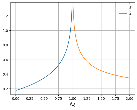
Figure 2: $z$ and $\tilde{z}$ are plotted as a function of the coupling strength ratio. Note that their value diverges at the critical region and the graphs are not mirror images of each other, there is an asymmetry.

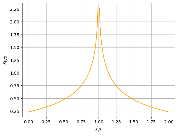
Figure 3: SVD entropy for $l$ and $r$ chiral degrees of freedom is plotted as a function of the coupling strength ratio. The entanglement entropy of the chiral degrees of freedom with the rest of the system diverges at the critical region.

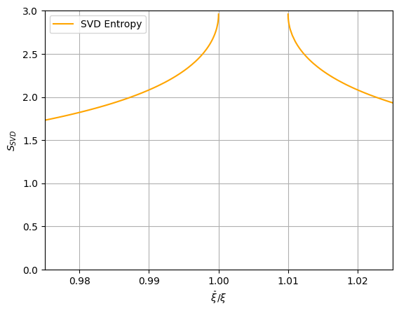
Figure 4: This figure shows more closely the graph for SVD entropy. Near the critical point, the values for SVD entropy become more valid. The point where the graph cuts off is where the value is diverging. Note that the asymmetry present in Figure 1 is also manifest here

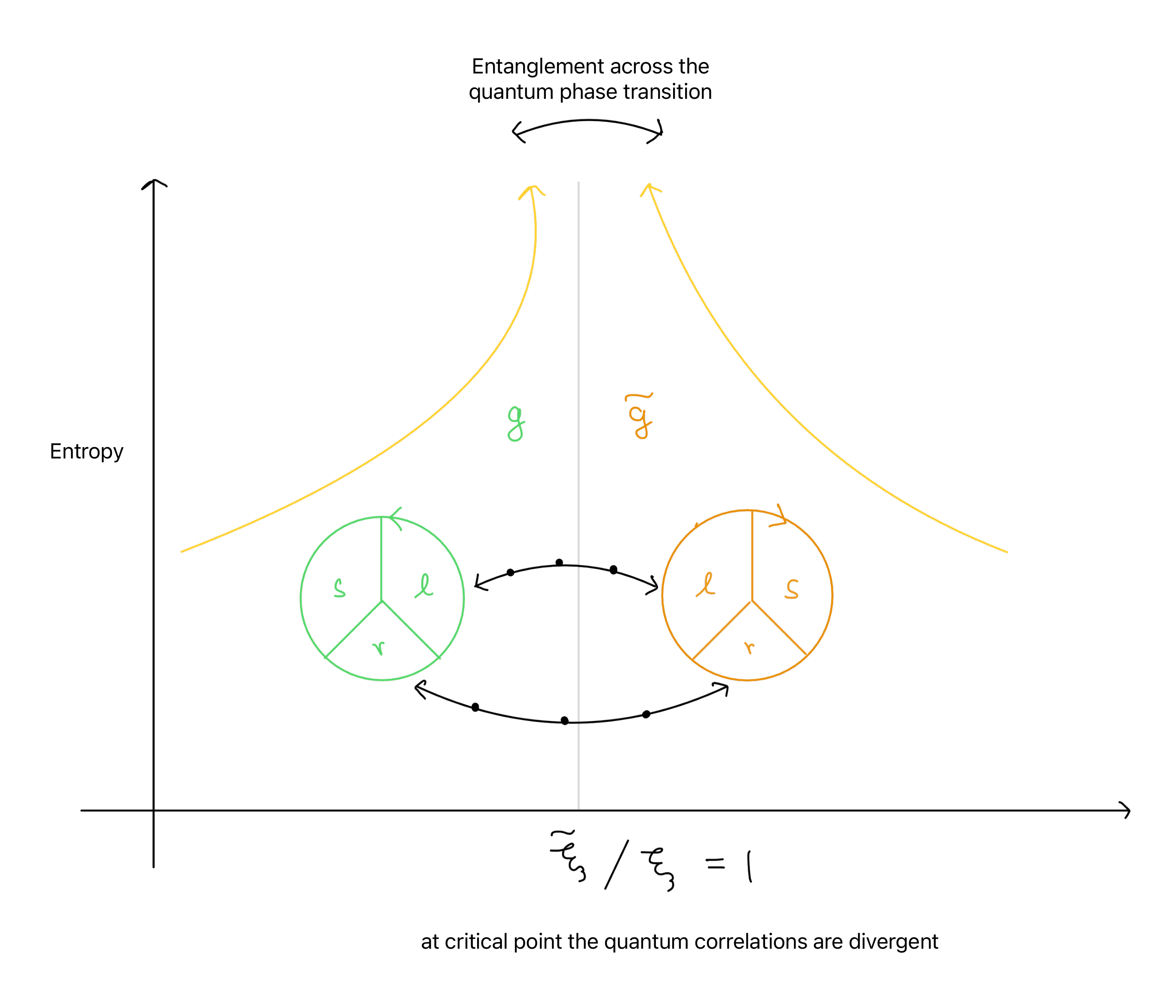
Figure 5: This is a rough sketch of Figure 4. The pie charts under the graph represent the degrees of freedom of the ground states ($l,r,s$). The dotted arrow line indicates entanglement for those degrees of freedom across the critical point. Since the SVD entanglement entropy for spinorial d.o.f. is 0, there is no arrow connecting those across the critical point.

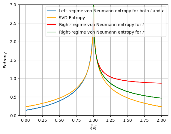
Figure 6: Comparison between SVD entropy and von Neumann entropy for different chiral degrees of freedom. For the left-handed regime, the von Neumann entropy for $l$ and $r$ degrees of freedom is equal [26]. Note how the values of left-regime von Neumann and the SVD entropy have the same behavior near the critical point.

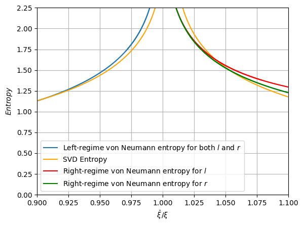
Figure 7: This figure shows more closely the comparison of behaviors between both the definitions of entropies.

The SVD entanglement entropy is plotted (Figure 3) by considering the values of $z$ and $\tilde{z}$ outside their domain as we have assumed $|z|\approx|\tilde{z}|$. The most accurate representation of SVD entanglement entropy is near the critical point (Figure 4). The schematic in Figure 5 explains the plot in Figure 4, it shows how the entanglement is across the states at the critical point in the quantum phase transition. Since at the critical point, we can assume that for some value of the coupling strength ratio near the critical point we have approximately equal values of $|z|$ and $|\tilde{z}|$. Numerically, we have taken the values of $\tilde{z}$ starting from the critical point and used those together with the values of $z$(starting from near the origin) to plot the graph for the left-hand side of Figure 3 and similarly, we have taken values from near the origin for $z$ along with values for $\tilde{z}$ (starting from the critical point) to plot the right-hand side of Figure 3.
As shown above for the $|z|\approx|\tilde{z}|$ case we see that the value for the SVD entanglement entropy matches the von Neumann entropy given in [26]. This becomes apparent near the critical point of the plot Figure 7. Figure 6 and Figure 7 is the plot for comparison between von Neumann and SVD entanglement entropy. Note that the value for SVD entanglement entropy is different in the right-handed regime, as compared to the results for von Neumann one. This is an important point of distinction between both the entropies. We also see that SVD entanglement entropy gives us one value for entropy for both $l$ and $r$ degrees of freedom and also for the left-handed and right-handed regime, which arguably makes it a better parameter to study quantum phase transition.

4 CONCLUSION AND DISCUSSION

We examined a relativistic spin-1/2 Dirac oscillator in a constant magnetic field. The relativistic Hamiltonian can be mapped to Jaynes-Cummings and anti–Jaynes-Cummings terms [26], describing interactions between the spinor and chirally intrinsic bosons. These models are crucial in several areas of theoretical and experimental research, and reveal the interplay between opposite chiralities. A. Bermudez et al. in [26] showed us two distinct phases under weak and strong magnetic fields, each with opposite chirality. In the intermediate regime, a complex interaction between chiralities leads to a quantum phase transition. In this work we discuss the entanglement entropy of the hybrid ground states obtained from this system across the phase transition in more detail using the SVD entanglement entropy.

The SVD entanglement entropy is a generalization of the von Neumann entropy. It uses a preselection and a post-selection state to calculate the entanglement entropy of the system. Arthur J. Parzygnat et al. in [2] extended the von Neumann entropy concept from density matrices to general square matrices, defining it as SVD entropy. They showed that SVD entropy possesses similar properties to von Neumann entropy, including additivity, invariance under two-sided independent unitary transformations, and a modified form of concavity. In addition to the examples provided in [2] we provided a general example (or proof) for SVD entanglement entropy of Bell states which turns out to be $\log 2$ similar to the von Neumann case.

The entanglement properties that were brought forth from the SVD definition, turned out to show reasonably similar behavior as the von Neumann case, the values diverge at the critical point which is indicative of the signature of a quantum phase transition. Hence, both definitions are qualitatively similar at times but quantitative differences occur. Further applications of SVD entanglement entropy can be seen in quantum information and quantum computation theory. A relation between entropy and computational complexity can be sought out through the SVD entanglement entropy between a quantum algorithm’s initial and final states. Further applications of SVD entanglement entropy as an indicator of phase transition can be done in a geometrical spacetime context, wherein the phase transition of a particular quantum field is triggered by geometric changes in the background spacetime.

Entanglement is seen as a measure of complexity from an information theory point of view [1], for the entanglement entropy to diverge at the critical point, it means that the complexity and the quantum correlations of the degrees of freedom are divergent due to entanglement between the degrees of freedom of left-handed and right-handed regime ground state. This sort of behavior intuitively makes sense in a classical system exhibiting phase transition, as at the critical point the system undergoes a transition hence the information at the critical point of the system is in-deterministic because of its transitory nature [27, 28, 29, 30]. For a quantum system, it is explicitly shown by our work and [26] how the phase transition happens using entropic calculations, through first principle rather than statistical arguments.

5 ACKNOWLEDGEMENT

One of the authors (YS) has been supported by the Summer Research Program-2024 by S.N. Bose National Centre for Basic Sciences, JD Block, Sector III, Salt Lake, Kolkata 7000106, India.

References

- [1] Michael A. Nielsen and Isaac L. Chuang “Quantum Computation and Quantum Information: 10th Anniversary Edition” Cambridge University Press, 2010
- [2] Arthur J Parzygnat, Tadashi Takayanagi, Yusuke Taki and Zixia Wei “SVD entanglement entropy” In Journal of High Energy Physics 2023.12 Springer, 2023, pp. 1–45
- [3] Song He, Jie Yang, Yu-Xuan Zhang and Zi-Xuan Zhao “Pseudo entropy of primary operators in -deformed CFTs” In Journal of High Energy Physics 2023.9 Springer, 2023, pp. 1–34
- [4] K Narayan “Further remarks on de Sitter space, extremal surfaces, and time entanglement” In Physical Review D 109.8 APS, 2024, pp. 086009
- [5] Kotaro Shinmyo, Tadashi Takayanagi and Kenya Tasuki “Pseudo entropy under joining local quenches” In Journal of High Energy Physics 2024.2 Springer, 2024, pp. 1–47
- [6] Wu-zhong Guo and Jiaju Zhang “Sum rule for the pseudo-Rényi entropy” In Physical Review D 109.10 APS, 2024, pp. 106008
- [7] Song He, Yu-Xuan Zhang, Long Zhao and Zi-Xuan Zhao “Entanglement and pseudo entanglement dynamics versus fusion in CFT” In Journal of High Energy Physics 2024.6 Springer, 2024, pp. 1–34
- [8] Hiroki Kanda et al. “Entanglement phase transition in holographic pseudo entropy” In Journal of High Energy Physics 2024.3 Springer, 2024, pp. 1–67
- [9] Sebastian Grieninger, Kazuki Ikeda and Dmitri E Kharzeev “Temporal entanglement entropy as a probe of renormalization group flow” In Journal of High Energy Physics 2024.5 Springer, 2024, pp. 1–19
- [10] Takanori Anegawa and Kotaro Tamaoka “Black Hole Singularity and Timelike Entanglement” In arXiv preprint arXiv:2406.10968, 2024
- [11] Pratik Nandy, Tanay Pathak and Masaki Tezuka “Probing quantum chaos through singular-value correlations in sparse non-Hermitian SYK model” In arXiv preprint arXiv:2406.11969, 2024
- [12] Wu-zhong Guo, Song He and Yu-Xuan Zhang “Relation between timelike and spacelike entanglement entropy” In arXiv preprint arXiv:2402.00268, 2024
- [13] Wu-zhong Guo, Yao-zong Jiang and Jin Xu “Pseudoentropy sum rule by analytical continuation of the superposition parameter” In arXiv preprint arXiv:2405.09745, 2024
- [14] Y. Nakata et al. “New holographic generalization of entanglement entropy” [arXiv:2005.13801] In Phys. Rev. D 103.2, 2021, pp. 026005
- [15] D. Itô, K. Mori and E. Carriere “An example of dynamical systems with linear trajectory” In Il Nuovo Cimento A (1965-1970) 51.4, 1967, pp. 1119–1121 DOI: 10.1007/BF02721775
- [16] M Moshinsky and A Szczepaniak “The Dirac oscillator” In Journal of Physics A: Mathematical and General 22.17, 1989, pp. L817 DOI: 10.1088/0305-4470/22/17/002
- [17] Peter A Ivanov, Diego Porras, Svetoslav S Ivanov and Ferdinand Schmidt-Kaler “Simulation of the Jahn–Teller–Dicke magnetic structural phase transition with trapped ions” In Journal of Physics B: Atomic, Molecular and Optical Physics 46.10 IOP Publishing, 2013, pp. 104003 DOI: 10.1088/0953-4075/46/10/104003
- [18] O. Panella and P. Roy “Quantum phase transitions in the noncommutative Dirac oscillator” In Phys. Rev. A 90 American Physical Society, 2014, pp. 042111 DOI: 10.1103/PhysRevA.90.042111
- [19] J.. Franco-Villafañe et al. “First Experimental Realization of the Dirac Oscillator” In Phys. Rev. Lett. 111 American Physical Society, 2013, pp. 170405 DOI: 10.1103/PhysRevLett.111.170405
- [20] Ituen B. Okon et al. “Spin and pseudospin solutions to Dirac equation and its thermodynamic properties using hyperbolic Hulthen plus hyperbolic exponential inversely quadratic potential” In Scientific Reports 11.1, 2021, pp. 892 DOI: 10.1038/s41598-020-77756-x
- [21] M.. Stetsko “Dirac oscillator and nonrelativistic Snyder-de Sitter algebra” In Journal of Mathematical Physics 56.1, 2015, pp. 012101 DOI: 10.1063/1.4905085
- [22] L. Menculini, O. Panella and P. Roy “Quantum phase transitions of the Dirac oscillator in a minimal length scenario” In Phys. Rev. D 91 American Physical Society, 2015, pp. 045032 DOI: 10.1103/PhysRevD.91.045032
- [23] R… Oliveira, R.. Maluf and C… Almeida “Exact solutions of the Dirac oscillator under the influence of the Aharonov–Casher effect in the cosmic string background” In Indian Journal of Physics, 2024 DOI: 10.1007/s12648-024-03079-6
- [24] Fabiano M. Andrade and Edilberto O. Silva “Effects of spin on the dynamics of the 2D Dirac oscillator in the magnetic cosmic string background” In The European Physical Journal C 74.12, 2014, pp. 3187 DOI: 10.1140/epjc/s10052-014-3187-6
- [25] K. Bakke “Rotating effects on the Dirac oscillator in the cosmic string spacetime” In General Relativity and Gravitation 45.10, 2013, pp. 1847–1859 DOI: 10.1007/s10714-013-1561-6
- [26] A. Bermudez, M.. Martin-Delgado and A. Luis “Chirality quantum phase transition in the Dirac oscillator” In Phys. Rev. A 77 American Physical Society, 2008, pp. 063815 DOI: 10.1103/PhysRevA.77.063815
- [27] D.. Landau and K. Binder “A Guide to Monte Carlo Simulations in Statistical Physics” Cambridge University Press, 2005
- [28] C.. Pethick and H. Smith “Bose-Einstein Condensation in Dilute Gases” Cambridge University Press, 2008
- [29] H.. Stanley “Introduction to Phase Transitions and Critical Phenomena” Oxford University Press, 1987
- [30] S. Sachdev “Quantum Phase Transitions” Cambridge University Press, 2011
- [31] R Banerjee and Subir Ghosh “Canonical transformations and soldering” In Physics Letters B 482.1-3 Elsevier, 2000, pp. 302–308
- [32] R Banerjee and Subir Ghosh “The chiral oscillator and its applications in quantum theory” In Journal of Physics A: Mathematical and General 31.36 IOP Publishing, 1998, pp. L603
- [33] Rabin Banerjee and Sarmishtha Kumar Chaudhuri “Dual composition of odd-dimensional models” In Physical Review D—Particles, Fields, Gravitation, and Cosmology 85.12 APS, 2012, pp. 125002
- [34] Hiroaki Kusunose, Jun-ichiro Kishine and Hiroshi M. Yamamoto “Emergence of chirality from electron spins, physical fields, and material-field composites” In Applied Physics Letters 124.26, 2024, pp. 260501 DOI: 10.1063/5.0214919
- [35] G.. Dunne, R. Jackiw and C.. Trugenberger “”Topological” (Chern-Simons) quantum mechanics” In Phys. Rev. D 41 American Physical Society, 1990, pp. 661–666 DOI: 10.1103/PhysRevD.41.661
- [36] G.. Horowitz and J.. Maldacena “The Black hole final state” [hep-th/0310281] In JHEP 02, 2004, pp. 008
- [37] D. Gottesman and J. Preskill “Comment on ‘The Black hole final state”’ [hep-th/0311269] In JHEP 03, 2004, pp. 026
- [38] S. Salek, R. Schubert and K. Wiesner “Negative conditional entropy of postselected states” [arXiv:1305.0932] In Phys. Rev. A 90.2, 2014, pp. 022116
- [39] J. Fullwood and A.. Parzygnat “On dynamical measures of quantum information” [arXiv:2306.01831] In arXiv, 2023
- [40] Y.-T. Tu, Y.-C. Tzeng and P.-Y. Chang “Rényi entropies and negative central charges in non-Hermitian quantum systems” [arXiv:2107.13006] In SciPost Phys. 12.6, 2022, pp. 194
- [41] X. Zhu et al. “Quantum measurements with preselection and postselection” [arXiv:1108.1608] In Phys. Rev. A 84.5, 2011, pp. 052111
- [42] C. Ferrie and J. Combes “How the result of a single coin toss can turn out to be 100 heads” [arXiv:1403.2362] In Phys. Rev. Lett. 113.12, 2014, pp. 120404
- [43] J. Combes, C. Ferrie, Z. Jiang and C.. Caves “Quantum limits on postselected, probabilistic quantum metrology” [arXiv:1309.6620] In Phys. Rev. A 89.5, 2014, pp. 052117
- [44] Y. Aharonov, D.. Albert and L. Vaidman “How the result of a measurement of a component of the spin of a spin-1/2 particle can turn out to be 100” In Phys. Rev. Lett. 60.15, 1988, pp. 1351–1354
- [45] R. Ramos, D. Spierings, I. Racicot and A.. Steinberg “Measurement of the time spent by a tunnelling atom within the barrier region” arXiv:1907.13523 In Nature 583.7817, 2020, pp. 529–532
- [46] D… Arvidsson-Shukur et al. “Quantum advantage in postselected metrology” arXiv:1903.02563 In Nat. Commun. 11.3775, 2020
- [47] N. Lupu-Gladstein et al. “Negative quasiprobabilities enhance phase estimation in quantum-optics experiment” In Phys. Rev. Lett. 128.22, 2022, pp. 220504
- [48] Charles H. Bennett, Herbert J. Bernstein, Sandu Popescu and Benjamin Schumacher “Concentrating partial entanglement by local operations” In Phys. Rev. A 53 American Physical Society, 1996, pp. 2046–2052 DOI: 10.1103/PhysRevA.53.2046
- [49] Rabin Banerjee and Debashis Chatterjee “Non-relativistic reduction of spinors, new currents and their algebra” In Nuclear Physics B 954 Elsevier, 2020, pp. 114994
- [50] A. Bermudez, M.. Martin-Delgado and E. Solano “Mesoscopic Superposition States in Relativistic Landau Levels” In Phys. Rev. Lett. 99 American Physical Society, 2007, pp. 123602 DOI: 10.1103/PhysRevLett.99.123602
- [51] A. Bermudez, M.. Martin-Delgado and E. Solano “Exact mapping of the Dirac oscillator onto the Jaynes-Cummings model: Ion-trap experimental proposal” In Phys. Rev. A 76 American Physical Society, 2007, pp. 041801 DOI: 10.1103/PhysRevA.76.041801
- [52] E.T. Jaynes and F.W. Cummings “Comparison of quantum and semiclassical radiation theories with application to the beam maser” In Proceedings of the IEEE 51.1, 1963, pp. 89–109 DOI: 10.1109/PROC.1963.1664
- [53] S.. Barnett and P.. Knight “Thermofield analysis of squeezing and statistical mixtures in quantum optics” In J. Opt. Soc. Am. B 2.3 Optica Publishing Group, 1985, pp. 467–479 DOI: 10.1364/JOSAB.2.000467
- [54] A.. Perelomov “Coherent states for arbitrary Lie group” In Communications in Mathematical Physics 26.3, 1972, pp. 222–236 DOI: 10.1007/BF01645091