Optical Diffusion Models for Image Generation
Abstract
Diffusion models generate new samples by progressively decreasing the noise from the initially provided random distribution. This inference procedure generally utilizes a trained neural network numerous times to obtain the final output, creating significant latency and energy consumption on digital electronic hardware such as GPUs. In this study, we demonstrate that the propagation of a light beam through a semi-transparent medium can be programmed to implement a denoising diffusion model on image samples. This framework projects noisy image patterns through passive diffractive optical layers, which collectively only transmit the predicted noise term in the image. The optical transparent layers, which are trained with an online training approach, backpropagating the error to the analytical model of the system, are passive and kept the same across different steps of denoising. Hence this method enables high-speed image generation with minimal power consumption, benefiting from the bandwidth and energy efficiency of optical information processing.
1 Introduction
Diffusion models create new samples that resemble their training sets by gradually undoing the diffusion process, which requires the learned reverse process to be applied numerous times[1]. While this method demonstrated unprecedented capabilities by producing highly realistic samples[2, 3, 4, 5, 6, 7, 8], it is also highly time-consuming and expensive in terms of energy consumption and computing resources since a high number of steps are required for generating each sample[2]. This prolonged processing time not only limits accessibility but also contributes to a significant environmental footprint.
Currently, generating new samples with diffusion models relies on electronic, general-purpose computing hardware such as GPUs or TPUs. However, due to the repetitive nature of the reversal process required in this task, deploying specialized hardware instead of general-purpose ones could significantly enhance the efficiency of sampling. For instance, the use of ASICs in cryptocurrency mining for hashing algorithms has demonstrated substantial improvements in computational speed and energy efficiency[9]. However, both GPUs and ASICs, among other electronic digital computers, face the same challenges like heat dissipation, energy consumption, and the diminishing returns of Moore’s Law, as transistors shrink and encounter quantum effects and physical limits that hinder further gains[10]. Therefore, exploring alternative computing modalities, such as optical computing—which offers high bandwidth and low loss—is increasingly important[11]. Optical computing has already shown promise in various applications, including high-speed data transmission and real-time signal processing. Optical computing addresses the inefficiencies of electronic hardware by leveraging the inherent parallelism that light allows for the simultaneous processing of multiple data channels, significantly speeding up the computational process. Several optical neural networks have been reported to perform complex calculations at reduced latency and energy consumption compared to traditional electronic systems [12].
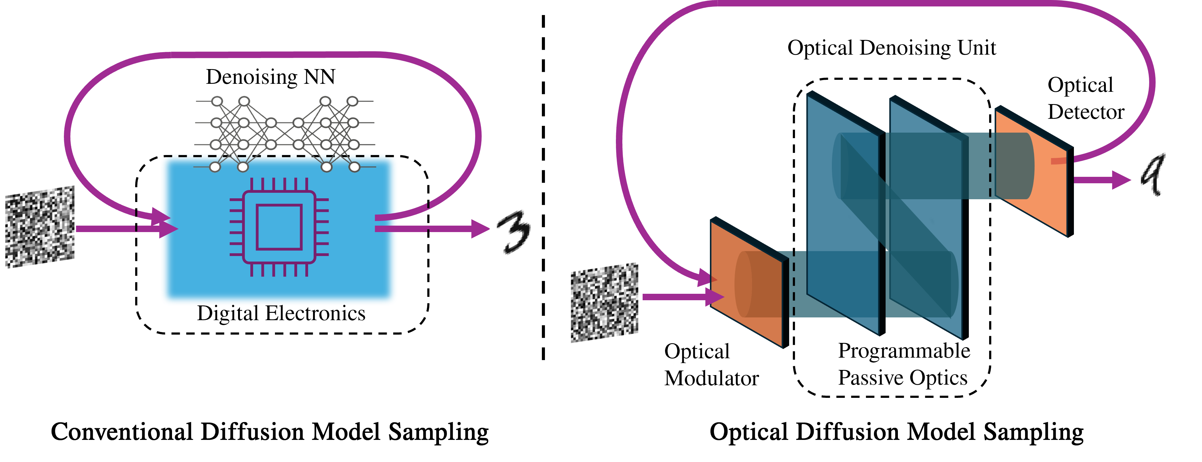
In this study, we demonstrate that optical wave propagation can be programmed to act as a computing engine specifically designed for implementing denoising diffusion models. As light passes through specially engineered transparent layers, features related to the original distribution are filtered out without any additional power consumption or computing latency, as depicted in Figure 1. This is due to the passive nature of the transparent layers, which are minimally absorptive and do not require active components or external power to function. These layers are designed to manipulate the light solely through their physical structure, which allows for the noise prediction to exit the system efficiently. Near zero energy consumption of passive optical components reduces the overall power requirements, making the system more energy-efficient.
Through iterative noise prediction and removal, this Optical Denoising Unit (ODU) can generate new images using a minimal number of these passive optical modulation layers. Because these layers do not need power or active control, they do not introduce any latency or energy overhead. Constrained only by optoelectronic input and readout hardware, this approach has the potential to significantly reduce the computational time and energy consumption of diffusion models. This technique opens up new avenues for performing inferences in more sustainable and scalable ways.
The main contributions of this study are:
-
•
The propagation of light through multiple modulation layers is programmed to perform denoising diffusion image generation by predicting and transmitting the noise term in the input images. The system uses only a single modulation plane and multiple reflections.
-
•
A time-aware denoising policy is specifically designed for analog optical computing hardware. This policy facilitates the use of passive building blocks to achieve multi-step computing at low power, translating the time-embedding in digital DDPMs into optical hardware.
-
•
An online learning algorithm is introduced for training ODUs in real-life scenarios, where alignment and calibration errors exist. The algorithm tracks and alleviates experimental discrepancies with constant updates to a digital twin during training time.
2 Related Work
Diffusion models have become popular, with their superior image generation performance compared to Generative Adversarial Networks (GANs). [13]. High-resolution, guided diffusion process is currently widely utilized for on-demand image generation[7, 6][14]. One of the main concerns with these highly capable models is the significant time taken for generating new samples, which can exceed 10 seconds for each high-resolution image [6]. Different methods have been proposed to alleviate this condition and improve the efficiency of diffusion models. While Latent Diffusion Models[6] work on a lower dimensional representation of images to decrease the computational load. Denoising Diffusion Implicit Models[15] introduce a deterministic and non-Markovian sampling process to reduce the number of required steps. Similarly, FastDPM [16], uses domain-specific conditional information for faster sampling with diffusion models. Another approach is to distill multiple denoising steps to a single one with a teacher-student setting[17]. As these methods aim to decrease iterative denoising steps required for sampling through algorithmic innovations, the potential improvements obtained by exploiting the repetitive nature of these models on the computing hardware side remain to be seen.
Optical processors have shown substantial energy efficiency improvements, particularly with larger model sizes, potentially outperforming current digital systems [18]. They can be implemented through various architectures, each leveraging different aspects of optical technology to perform computations. Free-space optical networks use spatial light modulators or fixed modulation layers for performing matrix multiplications and convolutions as light propagates[19, 20, 21], making them highly efficient for image processing tasks. These tasks include super-resolution[22], noise removal[23] an implementation of convolutional neural network layers[24]. On the other hand, photonic integrated circuits utilize optical components like Mach-Zehnder interferometers, microring resonators, and waveguides onto a single chip, enabling compact vector-matrix multipliers [25, 26]. Together, these developments highlight the transformative potential of optical computing in enhancing the performance and efficiency of computationally intensive tasks.
Considering the significant computational demands of denoising tasks, there is a clear need for specialized hardware to scale these operations effectively. Despite the advancements in optics, deep learning, and optical image processing, the realization of an optical diffusion denoiser remains a gap in current research. Bridging this gap could leverage the synergy between these fields to develop highly efficient and scalable solutions for denoising diffusion models.
In addition to their wide range of advantages, optical computing systems also have disadvantages related to the energy cost of modulation and detection of light, its limited programmability, and experimental precision. Therefore, it is crucial to perform as much as possible computations with the data while in the optical domain and carefully track experimental parameters. Final correction training[19] or a digital twin based experimental loss update[27] are the common solutions.
3 Description of the Study
3.1 Denoising Diffusion Models
DDPMs progressively corrupt data with Gaussian noise in a forward process and subsequently learn to reverse this corruption through a denoising process. This way they can generate new data samples that closely resemble the training data distribution. The forward diffusion process involves the sequential corruption of a data sample through the addition of Gaussian noise over timesteps. At each timestep , the data sample is perturbed to produce , , where is a variance schedule that determines the amount of noise added and is standard Gaussian noise. This process transforms the original data into nearly pure noise by timestep .
The reverse denoising process in DDPMs aims to reconstruct the original data from a highly noisy sample. Starting from completely Gaussian noise , the sample is iteratively denoised by removing the prediction of in the image, , which is provided by a trained neural network:
| (1) |
The training objective of the neural network can be simplified to minimize the mean squared error (MSE) between the true noise and the predicted noise where is uniformly sampled from . Finally, to generate new data samples, the model starts with a sample and applies the learned reverse transitions iteratively.
3.2 Propagation of Modulated Light Beams
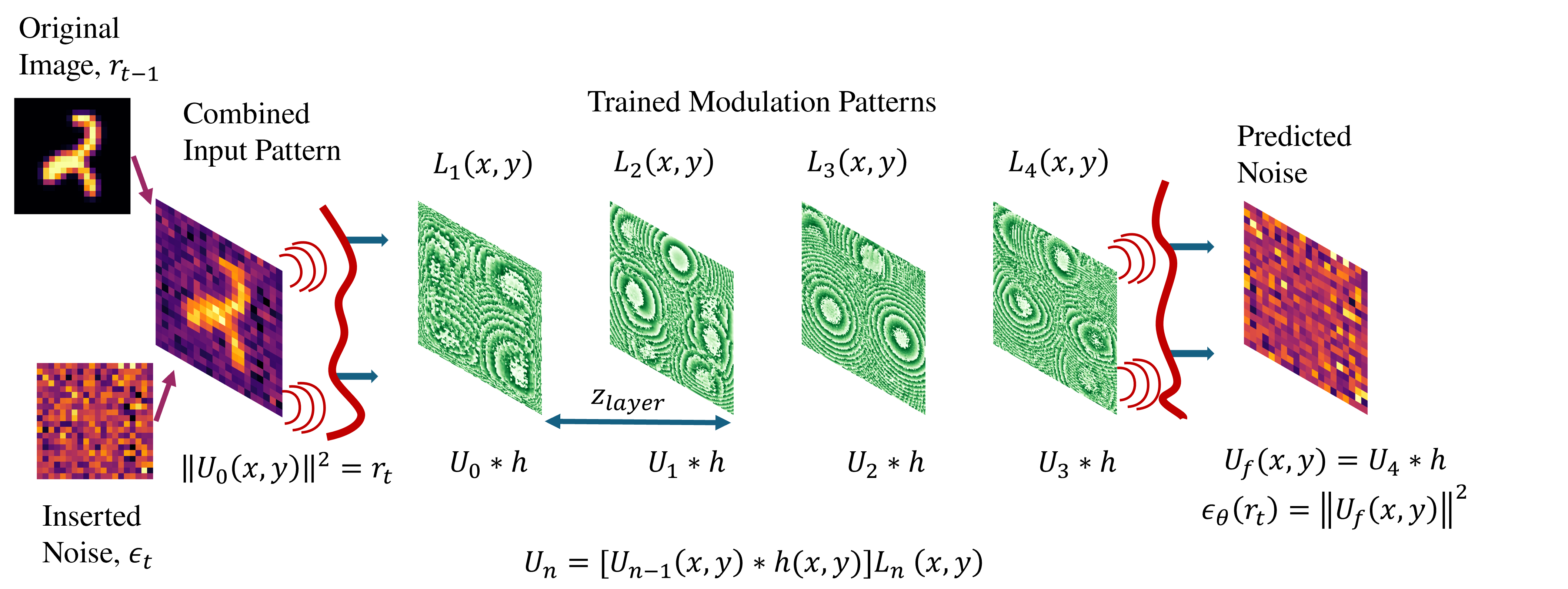
In this study, a denoising framework is presented by combining the modulation of a light beam with consequent transparent or reflective patterns and its propagation in free space (environments such as vacuum or air, where the refractive index of light is approximately 1), as shown in Figure 2. This process can be explained by the Fresnel diffraction theory since the features on the layers are not only larger than the optical wavelengths but only sufficiently smaller than the distance between different modulation layers [28]. According to this formalism, the electromagnetic field after propagating a distance in free space, , can be calculated from its distribution at by convolution with "the impulse response of free space", :
| (2) |
Here, denotes the wavenumber of the field, and is the wavelength. In other words, the field’s value at the plane of , at a given location , is the weighted sum of the values at , where the weight of each location is determined by the response function. Being complex numbers, all of these weights have the same magnitude but their phase depends on the location. In the frequency domain, the transfer function of free space becomes
| (3) |
This indicates that for spatial frequencies larger than , the magnitude of the transfer function reaches to zero exponentially. Hence, only features that are larger than the wavelength of the light can propagate to the far field. Moreover, frequency domain expression of diffraction, Equation 3, allows for also the efficient digital simulation of the propagation of light in free space with the utilization of Fast Fourier Transforms(FFTs) in a parallelized manner. Later on, we will benefit from this fact for GPU accelerated training of the diffractive modulation layers.
The proposed method applies trainable weights to the light beam at consequent planes with thin modulation layers. The interaction between layers and light can be represented as a point-wise multiplication between the incident field and the layer, which is followed by the propagation of the field in free space until the next layer,
| (4) |
where is the field distribution right before reaching the modulation layer , and is the complex modulation coefficient distribution of the trained modulation layers or the weights of the optical diffusion model. can be only a real number(), just phase modulation () or an arbitrary complex number depending on the implemented modulation principle. In this paper, we demonstrate our approach with a phase-only liquid crystal spatial light modulator (SLM), which can set to any value in the range of electronically, and everywhere.
3.3 Training of Optical Modulation Layers
As described in section 3.2, propagation of light can be analytically explained in a succinct manner for the scale considered in this study (). This allows for defining some free variables in this representation, such as refractive index distribution or input wavefront distribution , and optimizing these variables for minimizing a cost function. The gradients of these variables can be found with either manual calculation[29] or automatic differentiation packages[20]. In this study, our first goal is to find optimal modulation layers, or refractive index distributions, such that after the light beam encoded with the noisy images propagates through them only the predicted noise term reaches the detector, as shown in Figure 2. Moreover, the denoising network should be aware of the given timestep in the diffusion process while predicting the noise,, so that it would have a priori information about the variance of the noise term. Since noise level awareness is a crucial aspect of successful sample generation, most of the current implementations of diffusion models utilize time-embedding layers to modify activations of the neural network across different layers depending on the diffusion time step. Instead, the proposed method divides the diffusion timeline consisting of timesteps into subsets, and for each subset of time frames , trains a separate set of modulation layers each containing layers. Then, for , the noise prediction, becomes only a function of . In this scheme, the training objective for each time step is
| (5) |
where total loss is the sum over all ranges:
| (6) |
This decoupling of denoising at different timesteps by removing time-embedding layers also eliminates the necessity for digital computations to modifications at different layers. By circumventing this problem we perform denoising all-optically. Moreover, a fixed optical modulation pattern performs denoising at multiple consequent timesteps. For instance, we later demonstrate that for creates optimal results. So, a single layer set can process 100 timesteps and the entire sampling workflow can be operated with only 10 fixed parallel devices, or with only 10 updates to the SLM.
4 Results
4.1 All-Optical Denoising based Image Generation
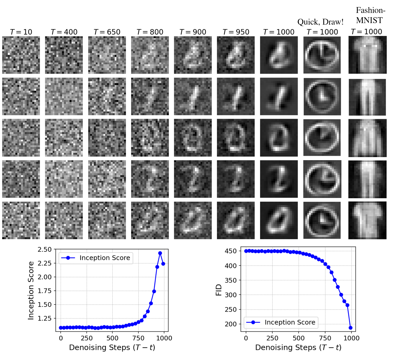
Following the same experimental settings with the initial DDPM study[2], we set , values to be in the linear range to . The results in Figure 3 are reported with the beam propagation model(Eqn.3) of the optical system designed to have 300x300 pixels per layer and four modulation layers. The number of layer sets (M) is 10. Denoising is over 1000 time steps. Several intermediate results are reported in Figure 3.
4.2 Effect of Optical Model Settings on the Image Denoising and Generation Performance
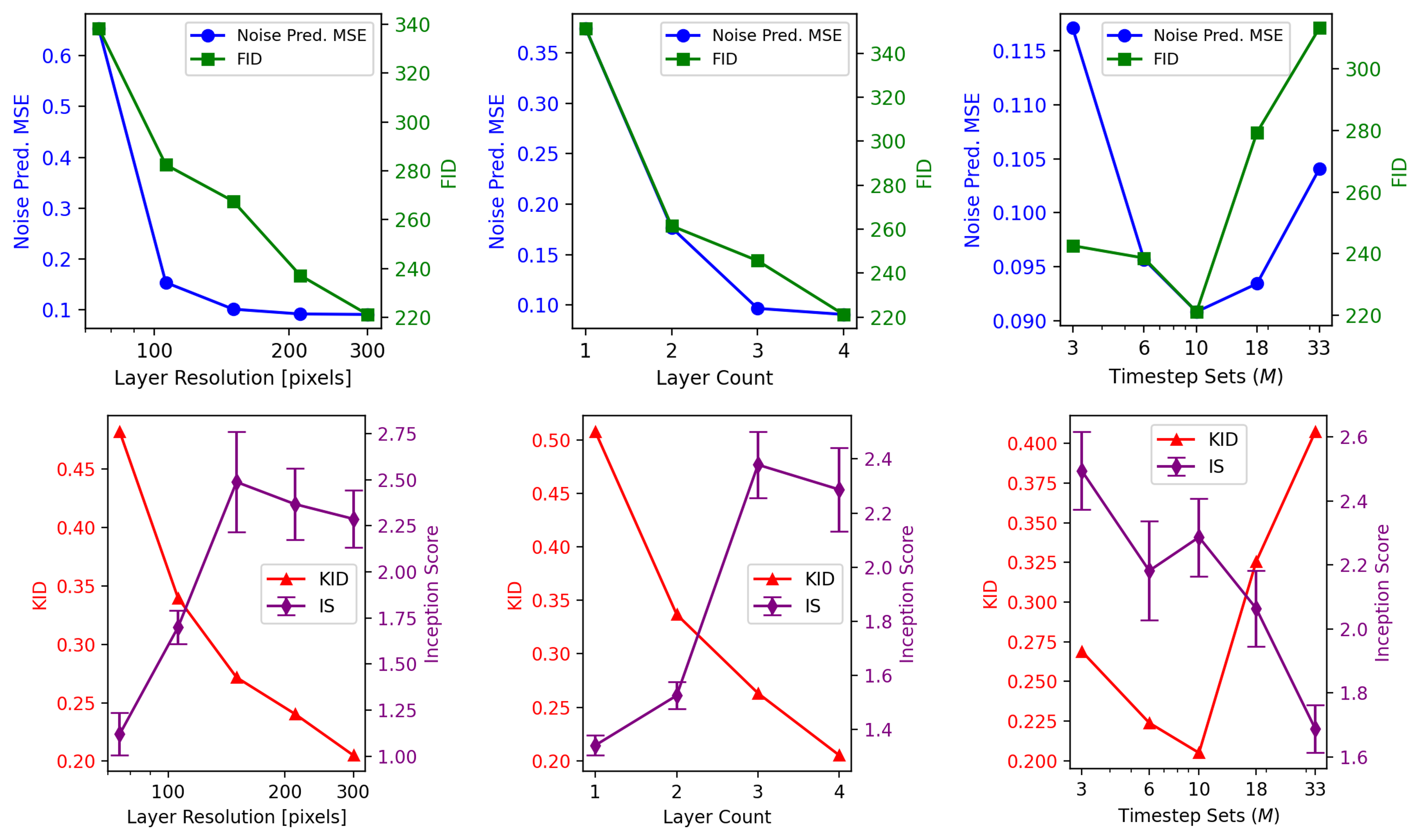
In our setting, there are three hyperparameters that control the total parameter count of the optical network: layer resolution, layer count, and timestep sets. We probe their effect over metrics: MSE: Mean Squared Error for denoising, FID: Fréchet Inception Distance, KID: Kernel Inception Distance, IS: Inception Score for generation task. In Figure 4, we observe that, as in digital neural networks, there is a clear tendency to perform better with a larger number of trainable parameters. Note that increasing layer resolution/count increases the total parameter count. On the other hand, having a larger number of denoising layers/timesteps improves the results only until they reach a certain level. Afterward, increasing the number of timestep is detrimental as shown in Figure 4. As the total number of training steps is fixed in this experiment, increasing the number of timesteps decreases the training sample count per layer set, hence potentially deteriorating the performance after a particular threshold, which is found to be M=10.
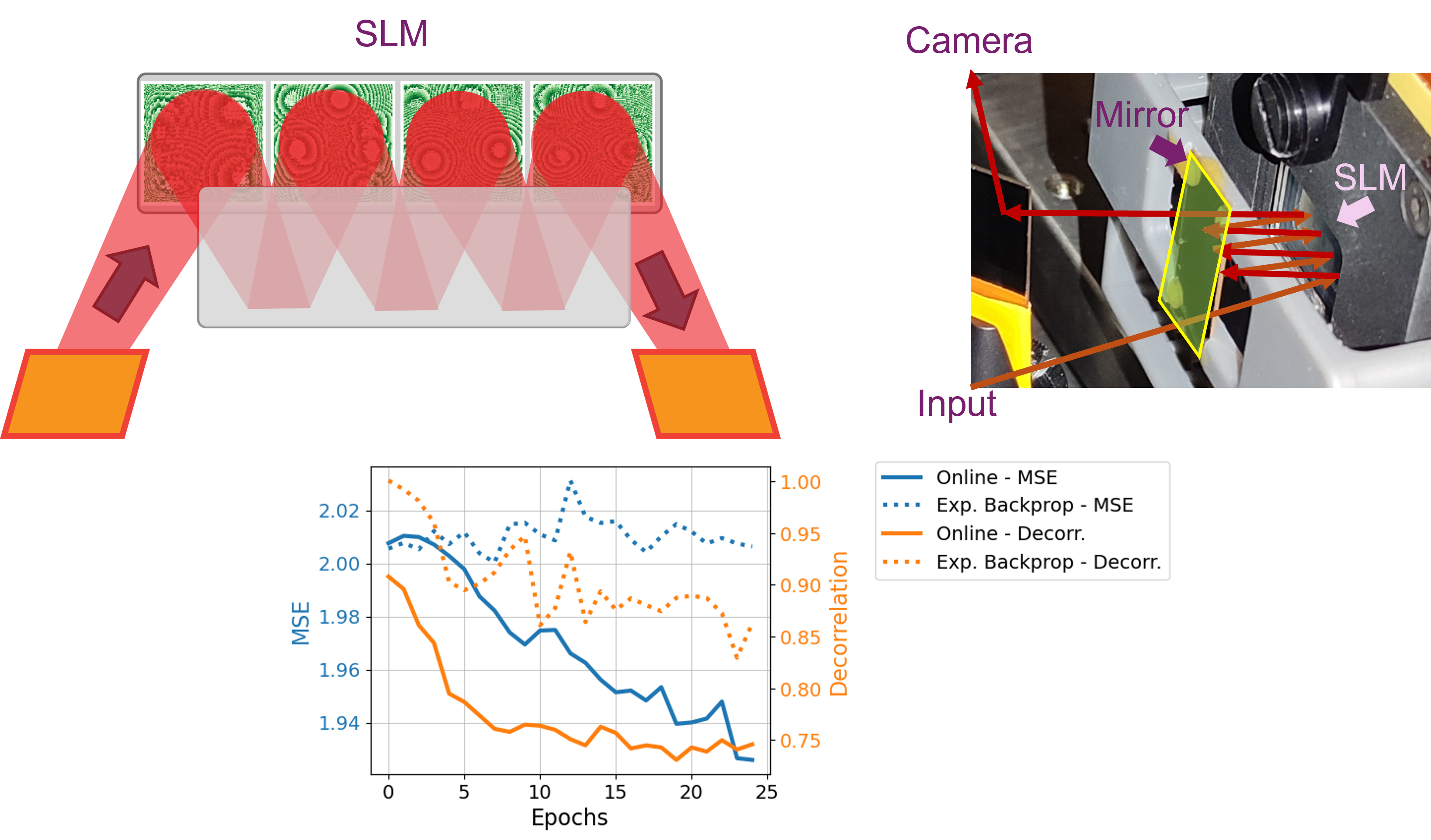
For resource-efficient prototyping, the proposed computing method, a single phase-only SLM and a mirror are paired in parallel to implement multiple modulation layers on a single device, as shown in Figure 5 and detailed in A.2.
Online Learning. To address the challenge of training an optical system with imperfect calibration, as faced in many other analog computing paradigms, we propose an online learning algorithm that updates and leverages a digital twin during training. During inference, the digital twin does not incur any additional overhead. The digital twin () again utilizes Fresnel diffraction based model of light propagation, as a surrogate to compute gradients and guide the optimization of the system’s trainable parameters. However, matching the digital twin’s parameters(), for instance, input beam angle, precise locations of the layers, and their angles, perfectly to the experimental conditions of the physical system is a challenging task. Therefore, during each iteration of training, the output of the experiment() and digital twin() is compared and the digital twin’s parameters are updated accordingly, as shown in 1.
In parallel, the digital twin is employed also to compute the gradients of the trainable parameters of the experiment, with respect to the output(). These gradients are then utilized to update the physical system’s parameters through backpropagation, informed by the error obtained from the physical system. Concurrently, the digital twin is refined using the latest inputs and outputs from the physical system to better approximate its behavior, despite the initial parameter mismatches. This iterative process of forward and backward passes, coupled with the continuous refinement of the digital twin, enables the physical system to progressively improve its performance and align more closely with the desired outcomes.
In Fig. 5, we explore the efficiency of the proposed algorithm by modeling a possible experiment scenario. The digital twin is calibrated to approximate an experiment, and a misalignment exists between its calibration and the actual experiment’s alignment, which is simulated by another diffraction model. We used 3 different algorithms, offline, experimental error backpropagation[27], and the proposed online training schemes. During training, MSE (training loss), and the discrepancy () between the digital twin and the experiment’s outputs are tracked. Offline training improves the loss function when evaluated with the digital twin, but when evaluated in the experimental setting, it has a higher MSE, as shown with a star in Fig. 5.
When the online training method is used, the digital twin is aligned with the actual experiment swiftly and the experimental loss approximates the MSE of perfect calibration case, the results of this approach with the optical experiment are also provided in Appendix 6. Backpropagating the experimental loss, MSE does not decrease significantly. However, for smaller misalignment, this method was also demonstrated to converge.

5 Conclusion
In this study, we introduced an optical diffusion denoising framework for image generation, utilizing a time-aware denoising strategy to optimize performance. By exploiting light propagation through transparent media, our Optical Denoising Unit (ODU) effectively reduces noise in images, offering a notable decrease in both energy use and computational demand compared to conventional digital methods. The integration of a time-aware policy enables the ODU to adjust light modulation dynamically according to different stages of the denoising process, thus improving image quality with efficient processing. Looking ahead, the incorporation of more complex and larger modulation layers and the exploration of nonlinear optical effects could enhance the functionality of the system. These potential improvements suggest promising directions for future research in expanding the range of applications for this technique.
The proposed method can utilize off-the-shelf consumer electronics such as digital micromirror devices that can be found in portable projectors for input modulation and CMOS cameras for recording output prediction. As analyzed in detail in A.4, these devices have the potential of implementing denoising steps on the order of microsecond latencies while consuming a few Watts only. With the utilization of high-speed light modulation technologies [31] million-frames-per-second-level denoising can be achieved again with Watt level energy consumption, while still utilizing the proposed approach for predicting noise in provided images.
Acknowledgments and Disclosure of Funding
This work was supported by Google Research under grant number 901381. We would like to thank the Research Computing Platform at EPFL and Google Cloud Services for providing access to compute units.
References
- [1] J. Sohl-Dickstein, E. Weiss, N. Maheswaranathan, and S. Ganguli, “Deep Unsupervised Learning using Nonequilibrium Thermodynamics,” in Proceedings of the 32nd International Conference on Machine Learning. PMLR, Jun. 2015, pp. 2256–2265, iSSN: 1938-7228. [Online]. Available: https://proceedings.mlr.press/v37/sohl-dickstein15.html
- [2] J. Ho, A. Jain, and P. Abbeel, “Denoising Diffusion Probabilistic Models,” in Advances in Neural Information Processing Systems, vol. 33. Curran Associates, Inc., 2020, pp. 6840–6851. [Online]. Available: https://proceedings.neurips.cc/paper/2020/hash/4c5bcfec8584af0d967f1ab10179ca4b-Abstract.html
- [3] Y. Song, J. Sohl-Dickstein, D. P. Kingma, A. Kumar, S. Ermon, and B. Poole, “Score-Based Generative Modeling through Stochastic Differential Equations,” Oct. 2020. [Online]. Available: https://openreview.net/forum?id=PxTIG12RRHS&utm_campaign=NLP%20News&utm_medium=email&utm_source=Revue%20newsletter
- [4] A. Q. Nichol and P. Dhariwal, “Improved Denoising Diffusion Probabilistic Models,” in Proceedings of the 38th International Conference on Machine Learning. PMLR, Jul. 2021, pp. 8162–8171, iSSN: 2640-3498. [Online]. Available: https://proceedings.mlr.press/v139/nichol21a.html
- [5] A. Jalal, M. Arvinte, G. Daras, E. Price, A. Dimakis, and J. Tamir, “Robust Compressed Sensing MRI with Deep Generative Priors,” Nov. 2021. [Online]. Available: https://openreview.net/forum?id=wHoIjrT6MMb
- [6] R. Rombach, A. Blattmann, D. Lorenz, P. Esser, and B. Ommer, “High-Resolution Image Synthesis with Latent Diffusion Models,” in 2022 IEEE/CVF Conference on Computer Vision and Pattern Recognition (CVPR). New Orleans, LA, USA: IEEE, Jun. 2022, pp. 10 674–10 685. [Online]. Available: https://ieeexplore.ieee.org/document/9878449/
- [7] C. Saharia, W. Chan, S. Saxena, L. Li, J. Whang, E. Denton, S. K. S. Ghasemipour, R. Gontijo-Lopes, B. K. Ayan, T. Salimans, J. Ho, D. J. Fleet, and M. Norouzi, “Photorealistic Text-to-Image Diffusion Models with Deep Language Understanding,” Oct. 2022. [Online]. Available: https://openreview.net/forum?id=08Yk-n5l2Al
- [8] C. Saharia, J. Ho, W. Chan, T. Salimans, D. J. Fleet, and M. Norouzi, “Image Super-Resolution via Iterative Refinement,” IEEE Transactions on Pattern Analysis and Machine Intelligence, vol. 45, no. 4, pp. 4713–4726, Apr. 2023, conference Name: IEEE Transactions on Pattern Analysis and Machine Intelligence. [Online]. Available: https://ieeexplore.ieee.org/document/9887996
- [9] S. Küfeoğlu and M. Özkuran, “Bitcoin mining: A global review of energy and power demand,” Energy Research & Social Science, vol. 58, p. 101273, Dec. 2019. [Online]. Available: https://www.sciencedirect.com/science/article/pii/S2214629619305948
- [10] C. E. Leiserson, N. C. Thompson, J. S. Emer, B. C. Kuszmaul, B. W. Lampson, D. Sanchez, and T. B. Schardl, “There’s plenty of room at the Top: What will drive computer performance after Moore’s law?” Science, vol. 368, no. 6495, p. eaam9744, Jun. 2020, publisher: American Association for the Advancement of Science. [Online]. Available: https://www.science.org/doi/10.1126/science.aam9744
- [11] G. Wetzstein, A. Ozcan, S. Gigan, S. Fan, D. Englund, M. Soljačić, C. Denz, D. A. B. Miller, and D. Psaltis, “Inference in artificial intelligence with deep optics and photonics,” Nature 2020 588:7836, vol. 588, no. 7836, pp. 39–47, Dec. 2020, 101 citations (Semantic Scholar/DOI) [2022-01-23] Publisher: Nature Publishing Group. [Online]. Available: https://www.nature.com/articles/s41586-020-2973-6
- [12] P. L. McMahon, “The physics of optical computing,” Nature Reviews Physics, vol. 5, no. 12, pp. 717–734, Dec. 2023, publisher: Nature Publishing Group. [Online]. Available: https://www.nature.com/articles/s42254-023-00645-5
- [13] P. Dhariwal and A. Q. Nichol, “Diffusion Models Beat GANs on Image Synthesis,” Nov. 2021. [Online]. Available: https://openreview.net/forum?id=AAWuCvzaVt
- [14] A. Ramesh, P. Dhariwal, A. Nichol, C. Chu, and M. Chen, “Hierarchical Text-Conditional Image Generation with CLIP Latents,” Apr. 2022. [Online]. Available: https://arxiv.org/abs/2204.06125v1
- [15] J. Song, C. Meng, and S. Ermon, “Denoising Diffusion Implicit Models,” Oct. 2020. [Online]. Available: https://openreview.net/forum?id=St1giarCHLP
- [16] Z. Kong and W. Ping, “On Fast Sampling of Diffusion Probabilistic Models,” Jun. 2021, arXiv:2106.00132 [cs]. [Online]. Available: http://arxiv.org/abs/2106.00132
- [17] T. Salimans and J. Ho, “Progressive Distillation for Fast Sampling of Diffusion Models,” Jun. 2022, arXiv:2202.00512 [cs, stat]. [Online]. Available: http://arxiv.org/abs/2202.00512
- [18] M. G. Anderson, S.-Y. Ma, T. Wang, L. G. Wright, and P. L. McMahon, “Optical Transformers,” Feb. 2023, arXiv:2302.10360 [physics]. [Online]. Available: http://arxiv.org/abs/2302.10360
- [19] T. Zhou, X. Lin, J. Wu, Y. Chen, H. Xie, Y. Li, J. Fan, H. Wu, L. Fang, and Q. Dai, “Large-scale neuromorphic optoelectronic computing with a reconfigurable diffractive processing unit,” Nature Photonics, vol. 15, no. 5, pp. 367–373, May 2021, number: 5 Publisher: Nature Publishing Group. [Online]. Available: https://www.nature.com/articles/s41566-021-00796-w
- [20] X. Lin, Y. Rivenson, N. T. Yardimci, M. Veli, Y. Luo, M. Jarrahi, and A. Ozcan, “All-optical machine learning using diffractive deep neural networks,” Science, vol. 361, no. 6406, pp. 1004–1008, Sep. 2018.
- [21] J. Hu, D. Mengu, D. C. Tzarouchis, B. Edwards, N. Engheta, and A. Ozcan, “Diffractive optical computing in free space,” Nature Communications, vol. 15, no. 1, p. 1525, Feb. 2024, publisher: Nature Publishing Group. [Online]. Available: https://www.nature.com/articles/s41467-024-45982-w
- [22] C. Isil, D. Mengu, Y. Zhao, A. Tabassum, J. Li, Y. Luo, M. Jarrahi, and A. Ozcan, “Super-resolution image display using diffractive decoders,” Science Advances, vol. 8, no. 48, p. eadd3433, Dec. 2022, publisher: American Association for the Advancement of Science. [Online]. Available: https://www.science.org/doi/10.1126/sciadv.add3433
- [23] C. Isil, T. Gan, F. O. Ardic, K. Mentesoglu, J. Digani, H. Karaca, H. Chen, J. Li, D. Mengu, M. Jarrahi, K. Akşit, and A. Ozcan, “All-optical image denoising using a diffractive visual processor,” Light: Science & Applications, vol. 13, no. 1, p. 43, Feb. 2024, publisher: Nature Publishing Group. [Online]. Available: https://www.nature.com/articles/s41377-024-01385-6
- [24] J. Chang, V. Sitzmann, X. Dun, W. Heidrich, and G. Wetzstein, “Hybrid optical-electronic convolutional neural networks with optimized diffractive optics for image classification,” Scientific Reports, vol. 8, no. 1, p. 12324, Aug. 2018, number: 1 Publisher: Nature Publishing Group. [Online]. Available: https://www.nature.com/articles/s41598-018-30619-y
- [25] Y. Shen, N. C. Harris, S. Skirlo, M. Prabhu, T. Baehr-Jones, M. Hochberg, X. Sun, S. Zhao, H. Larochelle, D. Englund, and M. Soljacic, “Deep learning with coherent nanophotonic circuits,” Nature Photonics, vol. 11, no. 7, pp. 441–446, Jun. 2017, 925 citations (Semantic Scholar/DOI) [2022-01-23] Publisher: Nature Publishing Group _eprint: 1610.02365.
- [26] A. N. Tait, T. Ferreira de Lima, M. A. Nahmias, H. B. Miller, H.-T. Peng, B. J. Shastri, and P. R. Prucnal, “Silicon Photonic Modulator Neuron,” Physical Review Applied, vol. 11, no. 6, p. 064043, Jun. 2019, publisher: American Physical Society. [Online]. Available: https://link.aps.org/doi/10.1103/PhysRevApplied.11.064043
- [27] L. G. Wright, T. Onodera, M. M. Stein, T. Wang, D. T. Schachter, Z. Hu, and P. L. McMahon, “Deep physical neural networks trained with backpropagation,” Nature, vol. 601, no. 7894, pp. 549–555, Jan. 2022, number: 7894 Publisher: Nature Publishing Group. [Online]. Available: https://www.nature.com/articles/s41586-021-04223-6
- [28] J. Goodman, Introduction to Fourier Optics, 4th ed. New York: W. H. Freeman, May 2017.
- [29] U. S. Kamilov, I. N. Papadopoulos, M. H. Shoreh, A. Goy, C. Vonesch, M. Unser, and D. Psaltis, “Learning approach to optical tomography,” Optica, vol. 2, no. 6, pp. 517–522, Jun. 2015, publisher: Optica Publishing Group. [Online]. Available: https://opg.optica.org/optica/abstract.cfm?uri=optica-2-6-517
- [30] A. Paszke, S. Gross, S. Chintala, G. Chanan, E. Yang, Z. DeVito, Z. Lin, A. Desmaison, L. Antiga, and A. Lerer, “Automatic differentiation in PyTorch,” Oct. 2017. [Online]. Available: https://openreview.net/forum?id=BJJsrmfCZ
- [31] C. L. Panuski, I. Christen, M. Minkov, C. J. Brabec, S. Trajtenberg-Mills, A. D. Griffiths, J. J. D. McKendry, G. L. Leake, D. J. Coleman, C. Tran, J. St Louis, J. Mucci, C. Horvath, J. N. Westwood-Bachman, S. F. Preble, M. D. Dawson, M. J. Strain, M. L. Fanto, and D. R. Englund, “A full degree-of-freedom spatiotemporal light modulator,” Nature Photonics, vol. 16, no. 12, pp. 834–842, Dec. 2022, publisher: Nature Publishing Group. [Online]. Available: https://www.nature.com/articles/s41566-022-01086-9
Appendix A Appendix / supplemental material
A.1 Scaling Study Results
| Number of Sets | Denoising MSE | IS | FID | KID | Number of Parameters |
|---|---|---|---|---|---|
| 3 | 0.118 | 2.29 | 245 | 0.27 | 1.1 M |
| 10 | 0.101 | 2.47 | 231 | 0.24 | 3.6 M |
| 33 | 0.105 | 1.71 | 306 | 0.40 | 11.9 M |
A.2 Details of the Experimental System
Pixel values represent trainable parameters on the modulation layers and are digitally adjusted using a computer model, as outlined in Appendix B. After optimizing these parameters on the computer, they are implemented across various layers in the experimental setup, utilizing the spatial light modulator (SLM). The beam generated by a continuous-wave dye laser (M-Squared Solstis 2000) at reaches the phase-only SLM (Meadowlark HSP 1920-500-1200) after reflecting from a digital micromirror device (DMD), which can be used for spatial amplitude modulation. After 4 reflections on the modulating area SLM, the beam is imaged onto a CMOS camera (FLIR BFS-U3-04S2M-CS). The operating wavelength is set at 850 nm. An 11.6 mm wide mirror, placed 17.1 mm from the SLM display, captures four reflections. To direct the input beam toward the SLM, 4F imaging was employed, transferring the beam from a digital micromirror device (DMD), which serves as a programmable aperture ensuring the beam’s alignment with the first modulation layer of the SLM. We assigned 260-by-260-pixel patches for the modulation layers on the SLM, which has a pixel pitch of . After the fourth reflection, the beam is imaged, and a CMOS camera records the output intensity as a 130-by-130-pixel image, where the camera’s pixel pitch is .
A.3 Online Learning and Experimental System
A.4 Scalability and Efficiency Outlook on Optical Diffusion Models
Considering the availability of commercial off-the-shelf components, the proposed architecture can be implemented using a Digital Micromirror Device (DMD) as the optoelectronic input device. For example, Texas Instruments’ DLP9500 can display 23,148 patterns per second at a resolution of 1920x1080, with an electrical consumption of 4.5 W at board level, including data transfer (i.e. loop back from the detector). When representing 8-bit images with superpixels, this device is capable of displaying images of 90x90. For more extensive scaling, multiple devices can be concatenated. However, for simplicity, we will consider 28x28 images. For comparison, our in-house U-net-based DDPM implemented for benchmarking generates a 28-by-28 Digit MNIST image in 0.58 seconds utilizing 1000 passes on a P100 GPU.where a single pass takes approximately 0.58 ms and consumes about 0.1 J. In contrast, in our ODU, a single pass can be executed in approximately . In the passive configuration, power consumption occurs at the optoelectronic input device, the read-out detector, and the light intensity required to provide a sufficient signal-to-noise ratio (SNR) at the detector. Specifically, the input device consumes approximately and the detector consumes per pass. The SNR, especially in the context of a digital device like a detector or an ADC (analog-to-digital converter), is typically calculated as where represents the number of bits. Considering the shot-noise-limited scenario, the required number of photons can be calculated using where accounts for a portion of light scattered out in passive layers and accounts for the conversion efficiency of the detector. Assuming 90% transmittance for each modulation layer and 50% efficiency for the detector, and using an 850 nm wavelength to calculate the energy of each photon: , the required energy for light is only a few picojoules, which is negligible compared to the energy consumption of optoelectronic devices. This comparison shows that the ODU’s energy consumption of is significantly lower than the 0.1 J required by conventional methods, making the ODU more than 400 times more energy-efficient.
A.5 Training of Modulation Layers
As shown in Fig.3, we utilized 3 different dataset for demonstrating the proposed approach.
-
•
First 3 digits from MNIST-digits
-
•
First 3 classes from Fashion-MNIST
-
•
20000 "Clock" images from Quick, Draw! dataset
After being downsampled to 20x20, the images are used for 250 epochs to train the ODUs, with a learning rate of 0.006, which took 10 hours on an A100 GPU.
A.6 Definition of Performance Metrics
Mean Squared Error (MSE)
| (7) |
where are the true values and are the predicted values.
Fréchet Inception Distance (FID)
| (8) |
where and are the mean and covariance of the feature vectors of the real and generated data, respectively.
Kernel Inception Distance (KID)
| (9) |
where is a polynomial kernel and is the Inception network function that extracts features.
Inception Score
| (10) |
where is the conditional label distribution given generated image and is the marginal distribution over all generated images.