1.4pt

Inverse Physics-Informed Neural Networks for transport models in porous materials

Abstract

Physics-Informed Neural Networks (PINN) are a machine learning tool that can be used to solve direct and inverse problems related to models described by Partial Differential Equations. This paper proposes an adaptive inverse PINN applied to different transport models, from diffusion to advection-diffusion-reaction problems. Once a suitable PINN is established to solve the forward problem, the transport parameters are added as trainable parameters. We find that, for the inverse problem to converge to the correct solution, the different components of the loss function (data misfit, initial conditions, boundary conditions and residual of the transport equation) need to be weighted adaptively as a function of the training iteration (epoch). Similarly, gradients of trainable parameters are scaled at each epoch accordingly. Several examples are presented for different test cases to support our PINN architecture and its scalability and robustness.

Contents

1. 1 Introduction
2. 2 Mathematical models
   1. 2.1 Heat equation
   2. 2.2 Advection-Diffusion-Reaction equation
   3. 2.3 Mobile-Immobile model
3. 3 Physics-Informed Neural Network
   1. 3.1 Inverse PINN
   2. 3.2 Adaptive inverse PINN
4. 4 Numerical results
   1. 4.1 Reference data
   2. 4.2 Pure diffusion
   3. 4.3 Advection Diffusion
   4. 4.4 Advection-diffusion with mobile-immobile
5. 5 Conclusions

1 Introduction

In recent years, Physics-Informed Neural Networks (PINNs) (see (Karniadakis et al., 2021) for a recent review) have attracted significant attention in mathematical modelling due to their ability to address direct and inverse problems governed by differential equations. This tool elegantly integrates the principles of physics-based differential models with the adaptability of neural network architectures.

On the one hand, PINNs offer a powerful framework for solving direct problems: those concerned with computing the solution of complex partial differential equations (PDEs) with defined initial and boundary conditions. Classical numerical techniques, such as finite difference methods, finite elements, virtual element schemes, and spectral methods, are well established. However, these methods may encounter difficulties when addressing problems characterised by high non-linearities, high dimensionality, or uncertainties in parameters or boundary conditions. To overcome these limitations, data-driven approaches have been explored. For example, Zhou et al. (2023) explored using deep neural networks with specialised activation functions for solving high-dimensional nonlinear wave equations. Sukumar and Srivastava (2022) proposed a geometry-aware PINN method specifically designed to enforce boundary conditions in complex domains. Extensions to integral equations also show promise, as demonstrated by Vitullo et al. (2024), where orthogonal decomposition is combined with neural networks.

On the other hand, PINNs can play a crucial role in solving inverse problems as surrogate models coupled with standard parameter estimation techniques (Bayesian or deterministic), or as stand-alone tools. In the first case, the independent variables and the physical parameters are treated as input to the neural network, which is trained for a wide range of physical parameters. In the second case, the physical parameters are treated as trainable neural network parameters. Although not directly appearing in the neural network, they are present in the loss function through the equation residual. In this work we will consider only this second approach which has been successfully applied to a wide range of problems, from groundwater flow and contaminant transport (Difonzo et al., 2024), to heat transfer in porous media (Yang et al., 2021), to the identification of unknown PDE structures (Gao et al., 2022). We will refer to this approach as inverse PINN. Inverse problems are inherently more complex than their direct counterparts due to their potential ill-posed nature, where multiple solutions might exist or none at all. Additional challenges arise from data-scarce regimes, irregular geometries (e.g., (Gao et al., 2022)), missing data, or uncertainties inherent to the model. Advanced PINN techniques have been developed to address these issues. Yang et al. (2021) introduced a Bayesian PINN framework for both inverse and forward models. Gusmão and Medford (2024) framed PINNs in terms of maximum-likelihood estimators, enabling error propagation and removing a hyperparameter. Finally, Difonzo et al. (2024) employs a serialised PINN approach to determine kernel functions in peridynamic models.

Data-driven and machine-learning approaches have found promising applications particularly in material modelling (Jeong et al., 2024; Guo et al., 2022; Upadhyay et al., 2024) and transport processes in porous media (Amini et al., 2022; Marcato et al., 2023; Santos et al., 2020). We refer to (D’Elia et al., 2022) and references therein for a recent review. Porous media are present in almost all aspects of engineering, manufacturing, and physical sciences. Porous media effective parameters (i.e. parameters controlling the emerging macroscopic dynamic of multi-scale materials) often have to be found by solving inverse problems. These include, for example, permeability, dispersivity and effective reactivity, which are crucial for agronomy, soil science and hydrological applications. Similar problems arise also in biology and medicine (tissues, bones, circulation network) and engineering (porous electrodes in batteries, concrete and building materials). Due to their multi-scale structure and heterogeneity and the availability of sparse heterogeneous data, data-driven models like PINN quickly gained popularity in these areas. Recent works also investigated the use of PINN for the identification of the effective parameters (He et al., 2020; Wang et al., 2023b; He and Tartakovsky, 2021).

This work proposes an adaptive inverse PINN architecture for solving advection-diffusion-reaction models. We consider a number of transport models, from simple diffusion to more complex advection-diffusion-reaction equations with the key parameters being dispersivity, effective velocity (a measure of permeability), and reaction constants. The main novelty of the proposed approach is the adaptive scaling of the loss function components and gradients of the trainable parameters. This adaptive scaling is crucial for the convergence of the inverse problem, as it ensures that the different components of the loss function are balanced and that the gradients of the trainable parameters are scaled appropriately. We demonstrate the effectiveness of the proposed approach through a series of numerical experiments, showing that the adaptive inverse PINN architecture is scalable, robust, and efficient for solving a wide range of transport models. In section 2, we introduce the mathematical models we consider, and in section 3, we present the PINN architecture we use. In section 4, we present the results of our numerical experiments, and in LABEL:sec:conclusions, we draw our conclusions.

2 Mathematical models

2.1 Heat equation

The simplest model we consider is a pure diffusion (heat) equation:

$$u_{t}-D\Delta u =0\,,\qquad x\in\Omega\,,\;t\in[0,T]\,,$$ (1)

and its non-linear extension:

$$u_{t}-\nabla\cdot(\mathcal{D}(u)\nabla u) =0\,,\qquad x\in\Omega\,,\;t\in[0,T]\,,$$ (2)

where $D$ is a constant diffusion coefficient, and $\mathcal{D}(u)$ is a non-linear diffusion coefficient.

2.2 Advection-Diffusion-Reaction equation

We consider the following advection-diffusion-reaction equation with non-linear reaction term:

$$\beta u_{t}+\nabla\cdot\left(Vu-D\nabla u\right) =\sigma(u)\,,\qquad x\in\Omega\,,\;t\in[0,T]\,,$$ (3)

with appropriate initial and boundary conditions. The spatial operator is a linear advection diffusion operator, with velocity $V$ and dispersion/diffusion coefficient $D$. The time-derivative involves a porosity term $\beta$. The reaction term $\sigma(u)$ is a non-linear function of the concentration $u$, which can be used to model a wide range of physical and chemical processes.

2.3 Mobile-Immobile model

The Mobile-Immobile model (Lapidus and Amundson, 1952) describes the transport of solutes in porous media and is based on the assumption that the solute is partitioned between a mobile and an immobile phase. The mobile phase is assumed to be in equilibrium with the immobile phase, and the transfer of solute between the two phases is described by a first-order rate equation. The model has been applied to a wide range of problems, including the transport of contaminants in groundwater, the transport of nutrients in soil, and the transport of solutes in fractured rock. For a recent review, derivation and extensions of the model we refer to (Municchi and Icardi, 2020b; Dentz et al., 2018). The model can be written as follows:

$$\beta_{0}u_{t}+\nabla\cdot\left(Vu-D\nabla u\right) =-\lambda(v-u)\,,\qquad x\in\Omega\,,\;t\in[0,T]\,,$$ (4)

$$\beta_{1}v_{t} =-\lambda(v-u)\,,\qquad x\in\Omega\,,\;t\in[0,T]\,,$$

where $\beta_{0}$ and $\beta_{1}$ are the mobile and immobile porosities, respectively, and $\lambda$ is the transfer coefficient.

3 Physics-Informed Neural Network

Figure 1: PINN structure used in this work, with $L$ layers, $m_{l}$ neurons per layer, and hyperbolic tangent activation function in the hidden layers.

In this paper, we will consider a Feed-Forward fully connected Neural Network (FF-DNN), also called Multi-Layer Perceptron (MLP) (see (Bengio et al., 2003; Cybenko, 1989) and references therein).
In a PINN, the solution space is approximated through a combination of activation functions, acting on all the hidden layers, with the independent variable used as the network input. Letting $(x,t)\in\mathbb{R}^{d+1}$ be the input of the NN, in a Feed-Forward network, each layer feeds the next one through a nested transformation so that it can be expressed, letting $L$ be the number of layers, as

$$z_{0} =(x,t),$$ (5)

$$z_{l} =\rho_{l}\left(\Lambda_{l}(z_{l-1})\right)\,,\qquad l=1,\ldots,L,$$

$$\Lambda_{l}(z_{l-1}) \coloneqq W_{l}z_{l-1}+b_{l}$$

where, for each layer $l=1,\ldots,L$, $\rho_{l}\mathrel{\mathop{\mathchar 58\relax}}\mathbb{R}^{m_{l}}\to\mathbb{R}^{m_{l}}$ is the activation function, which operates componentwise, $W_{l}\in\mathbb{R}^{m_{l}\times m_{l-1}}$ is the weight matrix and $b_{l}\in{\mathbb{R}^{m_{l}}}$ is the bias vector. Thus, the output $z_{L}\in\mathbb{R}^{m}$ of a FF-NN can be expressed as a single function of the input vector $x$, defined as the composition of all the layers above in the following way:

$$u_{NN}(x,t;\theta)=z_{L}\coloneqq(\sigma_{L}\circ\Lambda_{L}\circ\ldots\circ\sigma_{1}\circ\Lambda_{1})(x,t).$$

We denote the training parameters set as $\theta=\{W_{l},b_{l}\}_{l=1}^{L}$. In fig. 1, we show a schematic representation of the structure of a PINN, where the input layer is composed of two neurons, one for the spatial variable and one for the time variable, and the output layer is composed of a single neuron, resulting in the approximation $u_{NN}(x,t)$. The hidden layers are composed of the same number of neurons and the activation function used in the hidden layers is the hyperbolic tangent function, while the output layer uses the identity function. We have, therefore, $m_{0}=d+1$, $m_{L}=1$, and $m_{l}=m$ for $l=1,\ldots,9$. $\rho_{l}$ is the hyperbolic tangent function for $l=1,\ldots,L-1$, and the identity function for $l=L$. We will limit to one-dimensional spatial domain, i.e., $d=1$.

The aim of a PINN is to minimise a suitable objective function called loss function that includes not only the the data but also the physics of the problem. The minimisation is performed with respect to all the trainable parameters $\theta$, through a Stochastic Gradient Descent method. Given a general spatio-temporal differential operator $\mathcal{D}(u;\theta_{0})=0$, where $\mathcal{D}$ represents the differential operator acting on the unknown function $u\in V(\mathbb{R}^{d})$, with physical parameters $\theta_{0}\in\mathbb{R}^{s}$, the loss function used by a PINN is given by

$$\mathcal{L}(u;\theta_{0})\coloneqq\sum_{i=1}^{M}\left(\|u(x^{*}_{i},t^{*}_{i})-u^{*}_{i}\|^{2}+\|\mathcal{D}(u(x^{*}_{i},t^{*}_{i});\theta_{0})\|^{2}\right),$$ (6)

where $u^{*}_{i}$ is the unknown function measured at point $(x^{*}_{i},t^{*}_{i})$ inside the domain or on the boundary. The set $X^{*}=\{(x^{*}_{i},t^{*}_{i})\}_{i=1}^{M}$ is the set of training points, and $M$ is the number of training points that acts also as collocation points of the differential operator. In general training points and collocation points could be different but here we will consider the same set of points. The chosen norm $\|\cdot\|$ (it may be different for each term in the loss function) depends on the functional space and the specific problem. Selecting a correct norm (to avoid overfitting) for the loss function evaluation is an important problem in PINN, and recently, in (Taylor et al., 2023), the authors have proposed spectral techniques based on Fourier residual method to overcome computational and accuracy issues. The first term in the right-hand side of eq. 6 is referred to as data fitting loss and could possibly handle both initial and boundary conditions, while the second term is referred to as residual loss, which is responsible for making the NN informed by the physics of the problem. The derivatives inside $\mathcal{D}$ in space, time and in the parameter space are usually performed using autodiff (Automatic Differentiation algorithm, see (Baydin et al., 2017; Bolte and Pauwels, 2020)). Using the NN to approximate $u$ in the loss function eq. 6 allows us to solve the PDE by minimising the loss function with respect to the parameters $\theta$ of the NN. If $u\approx u_{NN}(\theta)$, then the minimisation problem can be written as

$$\theta^{\dagger}=\arg\min_{\theta}\mathcal{L}(u_{NN}(\theta);\theta_{0}).$$ (7)

For a more detailed discussion on the PINN structure and the loss function, we refer to (Raissi et al., 2019) and (Yang et al., 2021) and recent review in (Cuomo et al., 2022).

3.1 Inverse PINN

Inverse PINNs are a type of Neural Network specifically designed to determine constitutive parameters or problem-related functions that appear in the PDE one must solve. Because of their inherently ill-posedness, particular care has to be put into the training strategy during the optimization process. In particular, different contributions in the loss functions eq. 6 could conflict with each other, providing an unbalanced gradient back-propagation during the training, which would result in a troublesome convergence process (see (Xu et al., 2023)). Thus, several strategies have been recently developed to cope with these issues: among the others, one could resort to GradNorm (Haghighat et al., 2021) to dynamically tune gradient magnitudes to balance learning tasks; to PCGrad (Yu et al., 2020) to project each gradient on the tangent plane to all the other conflicting gradients to mitigate such destructive interference; to Multi-Objective Optimization (Sener and Koltun, 2018); to Self-Adaptive PINNs (McClenny and Braga-Neto, 2022), where each training point is weighed individually, so to penalize more points in difficult regions of the domain.

Using the notation introduced in the previous section, the inverse PINN minimisation now takes into account also the physical parameters and can be written as

$$(\theta^{\dagger},\theta_{0}^{\dagger})=\left[\arg\min_{\theta,\theta_{0}}\mathcal{L}(u_{NN}(\theta);\theta_{0})+\iota\|\theta_{0}-\theta_{0}^{*}\|^{2}\right],$$ (8)

where $\iota$ is a regularisation parameter. The second term in the right-hand side of the equation is the regularisation term, which is used to prevent overfitting and to ensure that the physical parameters $\theta_{0}$ are close to the some reference parameters $\theta_{0}^{*}$. If otherwise stated, in the following we will consider $\iota=0$.

3.2 Adaptive inverse PINN

To ensure the convergence of the inverse PINN, we redefine a weighted loss function as

$$\mathcal{L}(u_{NN}(\theta);\theta_{0})=\sum_{i=1}^{M}\left(\omega_{i}^{k}\|u(x^{*}_{i},t^{*}_{i})-u^{*}_{i}\|^{2}+\omega_{\mathcal{D}}^{k}\|\mathcal{D}(u(x^{*}_{i},t^{*}_{i});\theta_{0})\|^{2}\right),$$ (9)

where $\omega_{i}^{k}$ are weight factors that depends on the training iteration $i$. The weights are updated at each iteration to ensure that the different components of the loss function are balanced. The weights are updated using the following formula:

$$\omega_{i}^{k} =\frac{\hat{\omega}_{i}^{k}}{\sum_{j=1}^{M}\hat{\omega}_{j}^{k}+\hat{\omega}_{\mathcal{D}}^{k}}\,,\qquad i=1,\ldots,M\,,$$ (10)

$$\omega_{\mathcal{D}}^{k} =\frac{\hat{\omega}_{\mathcal{D}}^{k}}{\sum_{j=1}^{M}\hat{\omega}_{j}^{k}+\hat{\omega}_{\mathcal{D}}^{k}}\,,$$ (11)

$$\hat{\omega}_{i}^{k} =\begin{cases}\eta_{BC}&\text{if }x^{*}_{i}\in\partial\Omega\\ \eta_{IC}&\text{if }t^{*}_{i}=0\\ \nu(k)\eta_{u}&\text{if }(x^{*}_{i},t^{*}_{i})\text{ is a collocation point,}\\ 0&\text{otherwise.}\end{cases}\,,\qquad i=1,\ldots,M\,,$$ (12)

$$\hat{\omega}_{\mathcal{D}}^{k} =1,,$$ (13)

where $\eta_{BC}$, $\eta_{IC}$, and $\eta_{u}$ are the weights for the boundary conditions, initial conditions, and collocation points, respectively. The function $\nu_{k}$ is an increasing function of the epoch $k$, such that $\nu_{k}=0$ and $\nu_{k}\to 1$ as $k\to\infty$. This allows the PINN to be trained initially solely by the PDE residual. In the following, we will consider

$$\nu_{k}=\frac{{\tanh\left(10\left(\frac{{k-K/2-K_{0}}}{K}\right)\right)+1}}{2}\,,\qquad k=1,\ldots,K\,,$$ (14)

where $K$ is the total number of epochs, and $K_{0}$ is a threshold epoch before the weights are updated more significantly.

The gradients $\nabla_{\theta}\mathcal{L}$ and $\nabla_{\theta_{0}}\mathcal{L}$ are computed with the autodiff algorithm, and the latter (the gradients with respect to the physical parameters) are scaled by $\gamma\nu(k)$ at each iteration. The scaling of the gradients is crucial for the convergence of the inverse PINN, as it ensures that the physical parameters are updated only when data is included in the loss function. The parameters are then updated with the Adam optimiser, with a sequence of learning rates that decrease at each iteration according to the epoch $k$. Namely starting from a learning rate $\alpha_{0}$ at the first epoch, the learning rate is updated as:

$$\alpha_{k}={\alpha_{0}}\beta^{\left\lfloor\frac{k}{100}\right\rfloor}\,,$$ (15)

where $0.9<\beta<0.99$ is a constant factor.

4 Numerical results

In this section, we apply our PINN to different models arising from eq. 3 and eq. 4, under several assumptions and contiditions.

4.1 Reference data

We use the chebfun package to generate reference data for the PINN training. The package is based on the Chebyshev polynomial approximation, and it is particularly suited for the solution of differential equations. We use the package to generate reference data for the PINN training, and we compare the results obtained with the PINN with the reference data generated by chebfun.

The numerical solution are sampled at $N=100$ points in the spatial domain and $M=100$ points in the time domain. These are used both as training and collocation points. Before performing the inverse PINN training, we have tested the PINN architecture for the direct problems, and we have verified that the PINN is able to accurately solve the direct problems for given parameter values. These have not been reported here for brevity.

4.2 Pure diffusion

The first testcase we consider is the pure diffusion problem, described by eq. 1. We consider a one-dimensional spatial domain $\Omega=[0,1]$ and a time domain $[0,1]$. The initial condition is $u(x,0)=0$, and the boundary conditions are $u(0,t)=1$ and $\frac{\partial u}{\partial x}(1,t)=0$. This corresponds to a continuous source at the left boundary and a no-flux boundary condition at the right boundary. The diffusion coefficient and its initial estimate are chosen randomly between $0.1$ and $10$. We use the PINN to solve the direct problem, and we consider the diffusion coefficient $D$ as a trainable parameter. We use the reference data generated by chebfun to train the PINN.

We choose the following weights for the loss function: $\eta_{BC}=10$, $\eta_{IC}=10$, $\eta_{u}=1$. We choose a total of $K=5000$ epochs, and we start updating the parameters and threshold epoch $K_{0}=1000$. The initial learning rate is set to $\alpha_{0}=0.01$ , the gradient scaling factor is set to $\gamma=0.2$ and learning rate reduction factor is set to $\beta=0.95$.

Figure 2: Solution of the pure diffusion problem for the final parameter values. PINN approximation (continuous line) and reference data (dashed line). Concentration as a function of space for different times (left) and concentration as a function of time for different space locations (right).

Figure 3: Evolution of the diffusion coefficient during training of PINN (left) and gradients of the diffusion coefficient (right).

Figure 4: Evolution of the weighted (left) and unweighted (right) loss functions during training of PINN.

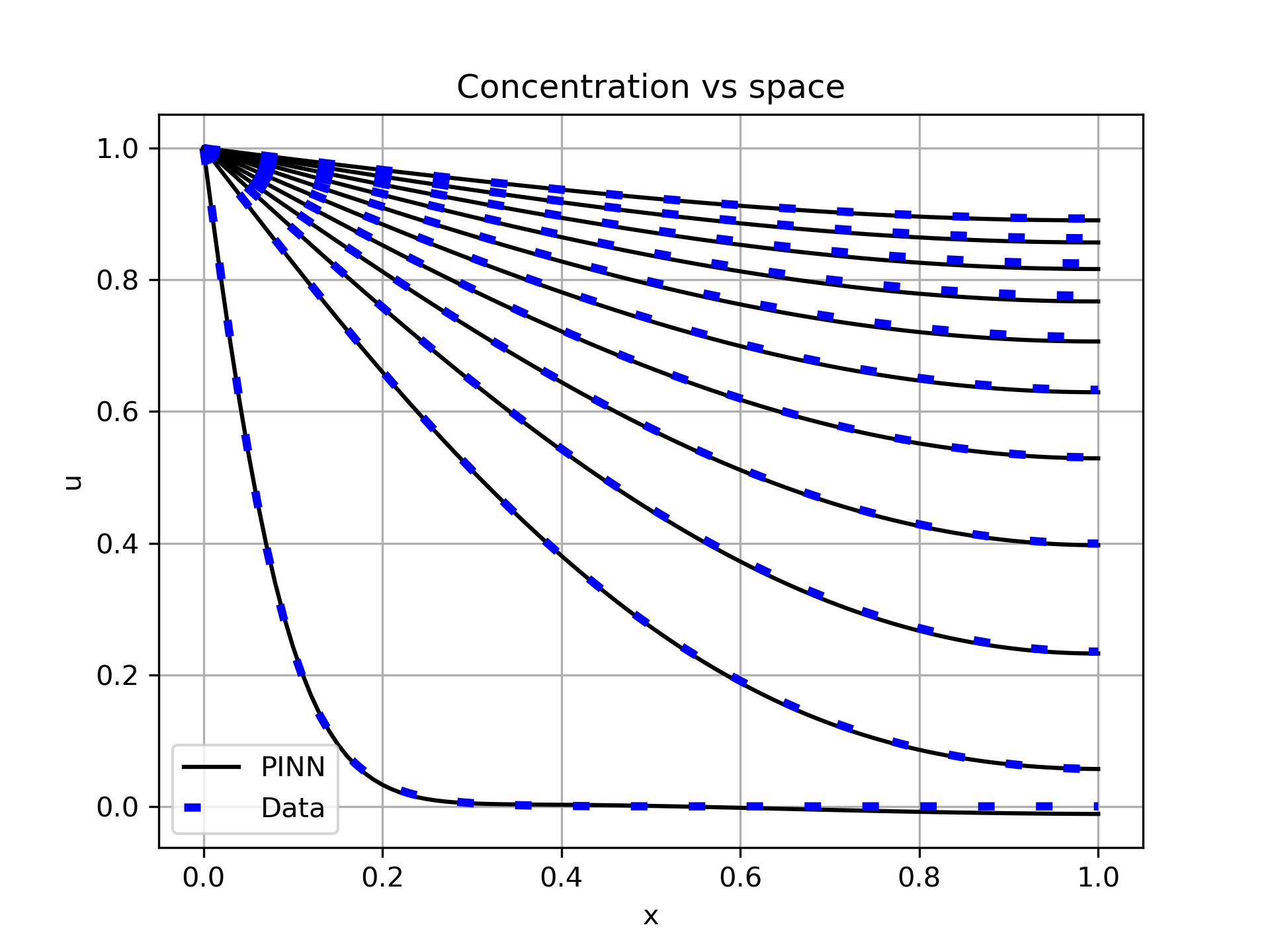
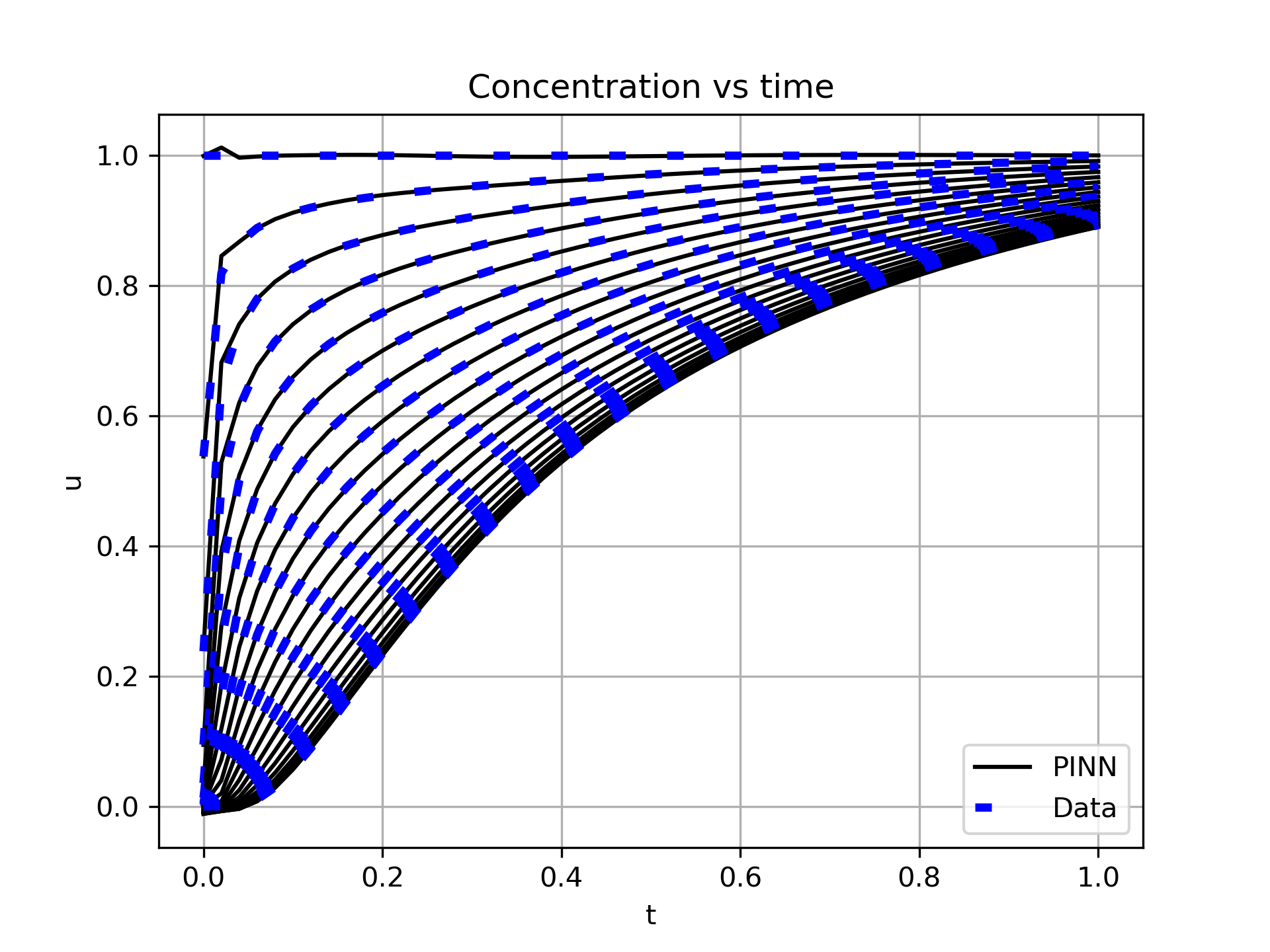
In fig. 2, we show the solution of the pure diffusion problem obtained with the PINN. The solution is compared with the reference data generated by chebfun. The solution is shown as a function of space for different times (left) and as a function of time for different space locations (right). The solution obtained with the PINN is in good agreement with the reference data, showing that the PINN is able to accurately solve the direct problem.

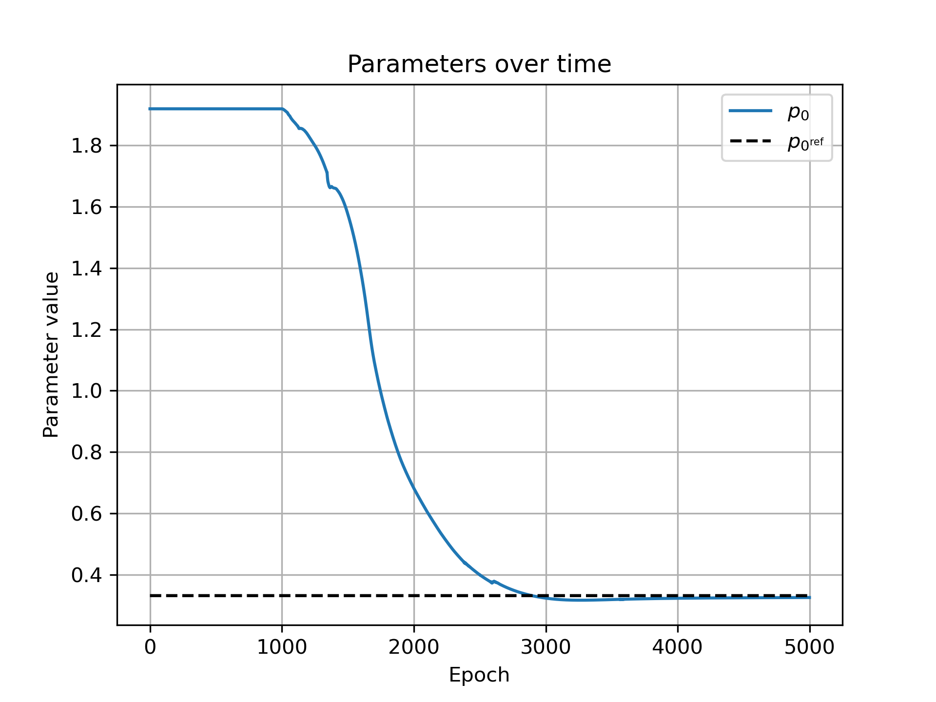
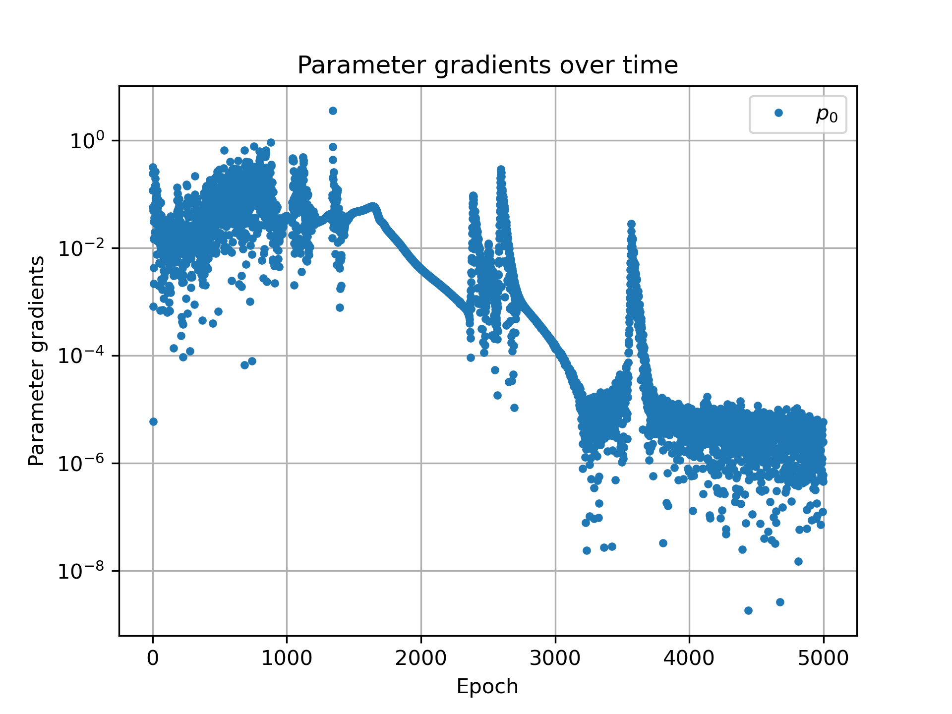
In fig. 3, we show the evolution of the diffusion coefficient during the training of the PINN. The diffusion coefficient is shown as a function of the training iteration (epoch). The diffusion coefficient is updated during the training of the PINN, and it converges to the correct value. The gradients of the diffusion coefficient are also shown as a function of the training iteration (epoch). The gradients are scaled at each epoch to ensure that the diffusion coefficient is updated correctly.

In fig. 4, we show the evolution of the weighted and unweighted loss functions during the training of the PINN. The weighted loss function is shown as a function of the training iteration (epoch), and it is updated at each epoch to ensure that the different components of the loss function are balanced. The unweighted loss function is also shown as a function of the training iteration (epoch), to better highlight the effect of the weighting factors.

4.3 Advection Diffusion

This testcase considers the advection-diffusion problem described by eq. 3. We consider a one-dimensional spatial domain $\Omega=[0,1]$ and a time domain $[0,1]$. The initial condition is $u(x,0)=0$, and the boundary conditions are $u(0,t)=H(0.01-t)$ and $\frac{\partial u}{\partial x}(1,t)=0$. This corresponds to a finite impulse at the left boundary and a no-flux boundary condition at the right boundary. The advection velocity and the dispersion coefficient are chosen randomly between 0.1 and 10, and the reaction term is here set to 0. We use the PINN to solve the direct problem, and we consider the advection velocity $V$ and the dispersion coefficient $D$ as trainable parameters. We use the reference data generated by chebfun to train the PINN.

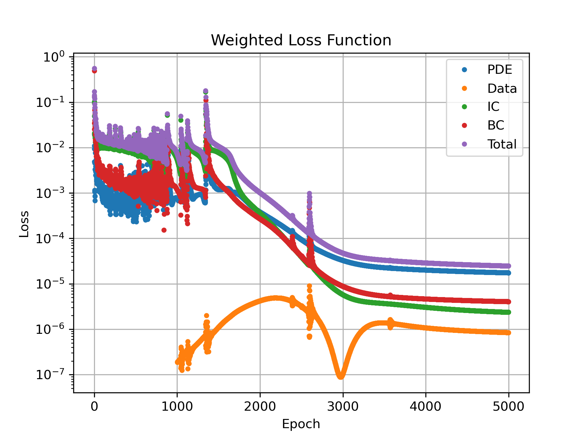
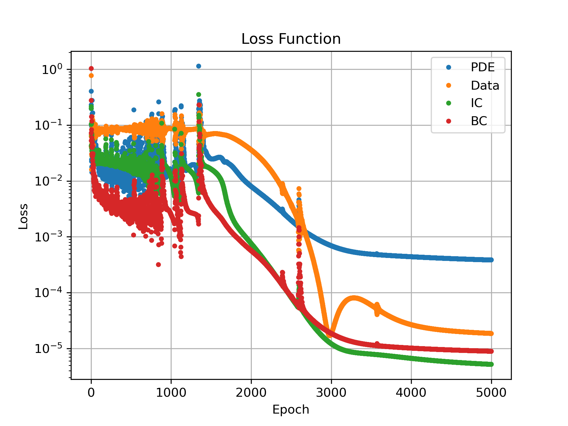
We choose the following weights for the loss function: $\eta_{BC}=10$, $\eta_{IC}=10$, $\eta_{u}=2$. We choose a total of $K=10000$ epochs, and we start updating the parameters and threshold epoch $K_{0}=1000$. The initial learning rate is set to $\alpha_{0}=0.01$ , the gradient scaling factor is set to $\gamma=0.2$ and learning rate reduction factor is set to $\beta=0.95$.

Figure 5: Solution of the advection-diffusion problem for the final parameter values.. PINN approximation (continuous line) and reference data (dashed line). Concentration as a function of space for different times (left) and concentration as a function of time for different space locations (right).

Figure 6: Evolution of the advection velocity and dispersion coefficient during training of PINN (left) and gradients of the advection velocity and dispersion coefficient (right).

Figure 7: Evolution of the weighted (left) and unweighted (right) loss functions during training of PINN.

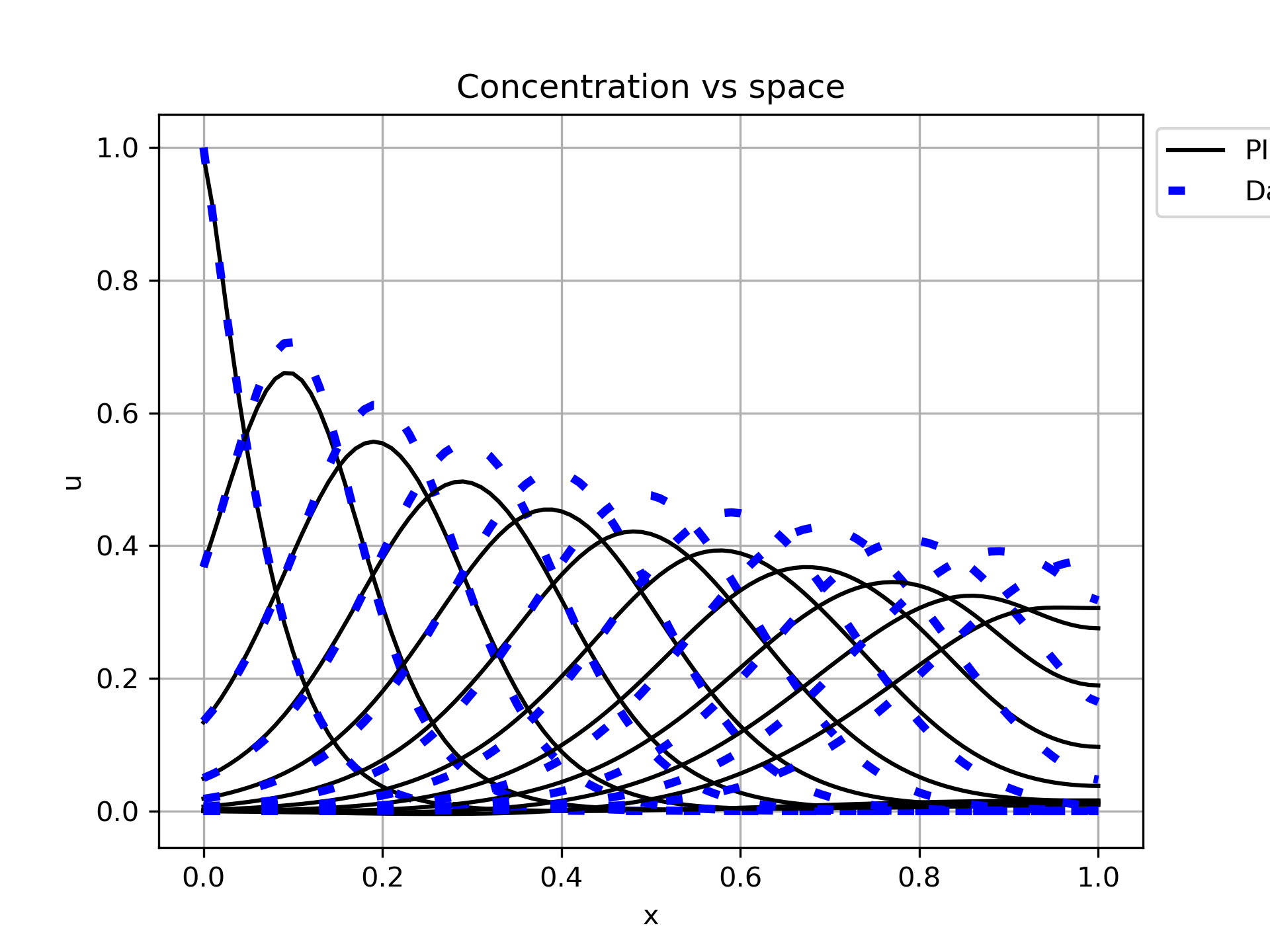
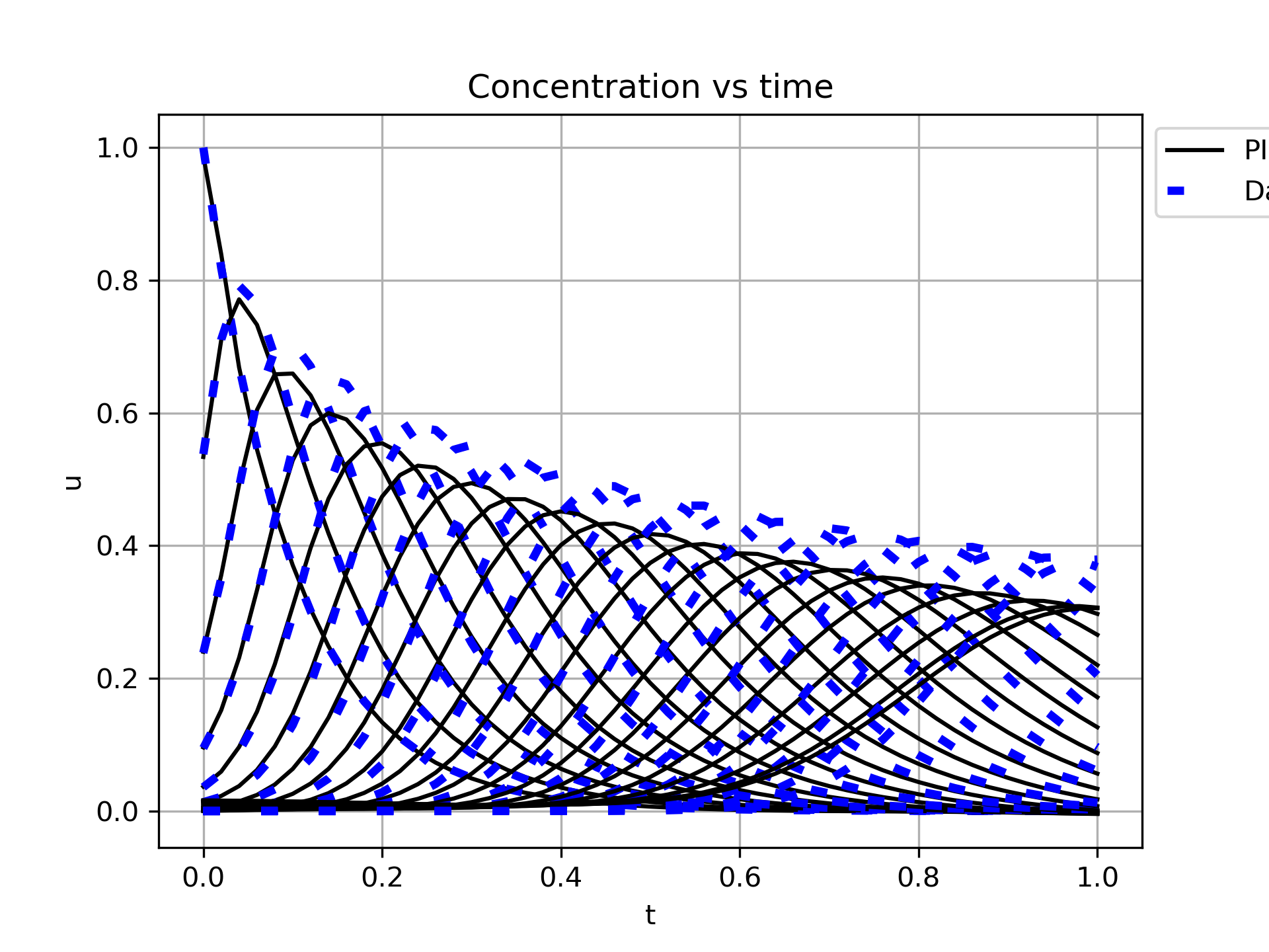
In fig. 5, we show the solution of the advection-diffusion problem obtained with the PINN. The solution is compared with the reference data generated by chebfun. The solution is shown as a function of space for different times (left) and as a function of time for different space locations (right). The solution obtained with the PINN is in good agreement with the reference data, showing that the PINN is able to accurately solve the direct problem.

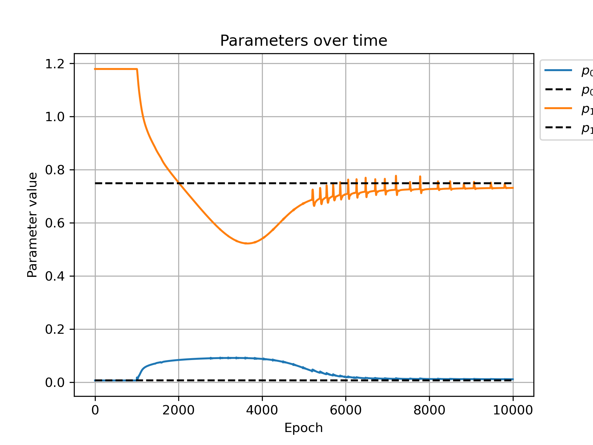
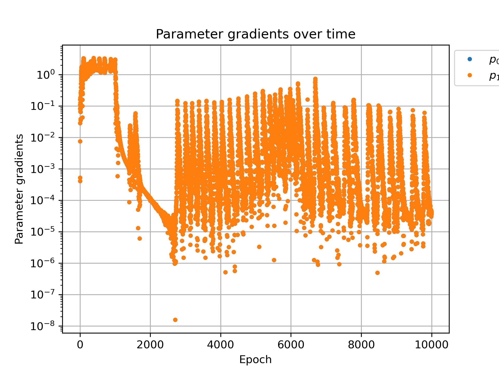
In fig. 6, we show the evolution of the advection velocity and dispersion coefficient during the training of the PINN. The advection velocity and dispersion coefficient are shown as a function of the training iteration (epoch). The advection velocity and dispersion coefficient are updated during the training of the PINN, and they converge to the correct values. The gradients of the advection velocity and dispersion coefficient are also shown as a function of the training iteration (epoch). The gradients are scaled at each epoch to ensure that the advection velocity and dispersion coefficient are updated correctly.

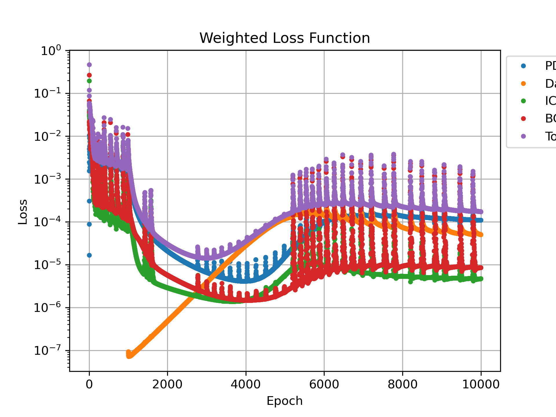
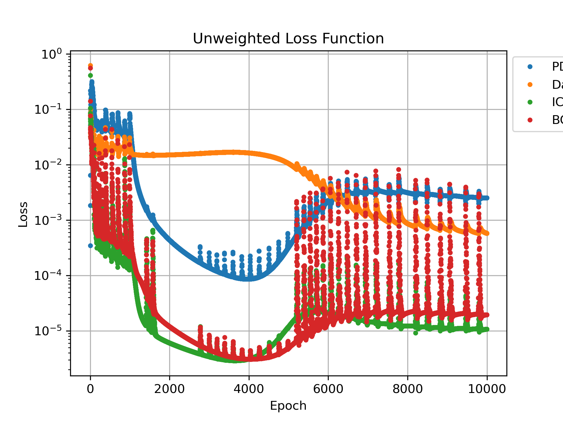
In fig. 7, we show the evolution of the weighted and unweighted loss functions during the training of the PINN. The weighted loss function is shown as a function of the training iteration (epoch), and it is updated at each epoch to ensure that the different components of the loss function are balanced. The unweighted loss function is also shown as a function of the training iteration (epoch), to better highlight the effect of the weighting factors.

4.4 Advection-diffusion with mobile-immobile

This testcase considers the advection-diffusion problem with mobile-immobile model described by eq. 4. We consider a one-dimensional spatial domain $\Omega=[0,1]$ and a time domain $[0,1]$. The initial condition is $u(x,0)=v(x,0)=0$, and the boundary conditions are $u(0,t)=1$ and $\frac{\partial u}{\partial x}(1,t)=0$. This corresponds to a continuous injection at the left boundary and a no-flux boundary condition at the right boundary. The effect of the immobile phase is to delay the transport of the solute, and the transfer coefficient $\lambda$ controls the transfer of solute between the mobile and immobile phases, resulting in long tails and non-Fickian transport behaviour (Municchi et al., 2021). The mobile and immobile porosities are fixed to $\beta_{0}=0.3$ and $\beta_{1}=0.1$, respectively, while dispersivity, effective velocity and transfer coefficient are the parameters to be estimated. The true values used for the training set are $D=0.1$, $V=1$, and $\lambda=10$. We use the PINN to solve the direct and inverse problem, and we consider the dispersion coefficient $D$, the effective velocity $V$, and the transfer coefficient $\lambda$ as trainable parameters. We use the reference data generated by chebfun to train the PINN. The initial values for the parameters are chosen randomly between 0.1 and 10.

We choose the following weights for the loss function: $\eta_{BC}=10$, $\eta_{IC}=10$, $\eta_{u}=1$. We choose a total of $K=10000$ epochs, and we start updating the parameters and threshold epoch $K_{0}=2000$. The initial learning rate is set to $\alpha_{0}=0.01$ , the gradient scaling factor is set to $\gamma=0.1$ and learning rate reduction factor is set to $\beta=0.98$.

Figure 8: Solution of the advection-diffusion with mobile-immobile model for the final parameter values. Mobile concentration. PINN approximation (continuous line) and reference data (dashed line). Concentration as a function of space for different times (left) and concentration as a function of time for different space locations (right).

Figure 9: Solution of the advection-diffusion with mobile-immobile model for the final parameter values.. Immobile concentration. PINN approximation (continuous line) and reference data (dashed line). Concentration as a function of space for different times (left) and concentration as a function of time for different space locations (right).

Figure 10: Evolution of the relative error in the dispersion coefficient, effective velocity, and transfer coefficient during training of PINN (left) and gradients of the dispersion coefficient, effective velocity, and transfer coefficient (right).

Figure 11: Evolution of the weighted (left) and unweighted (right) loss functions during training of PINN.

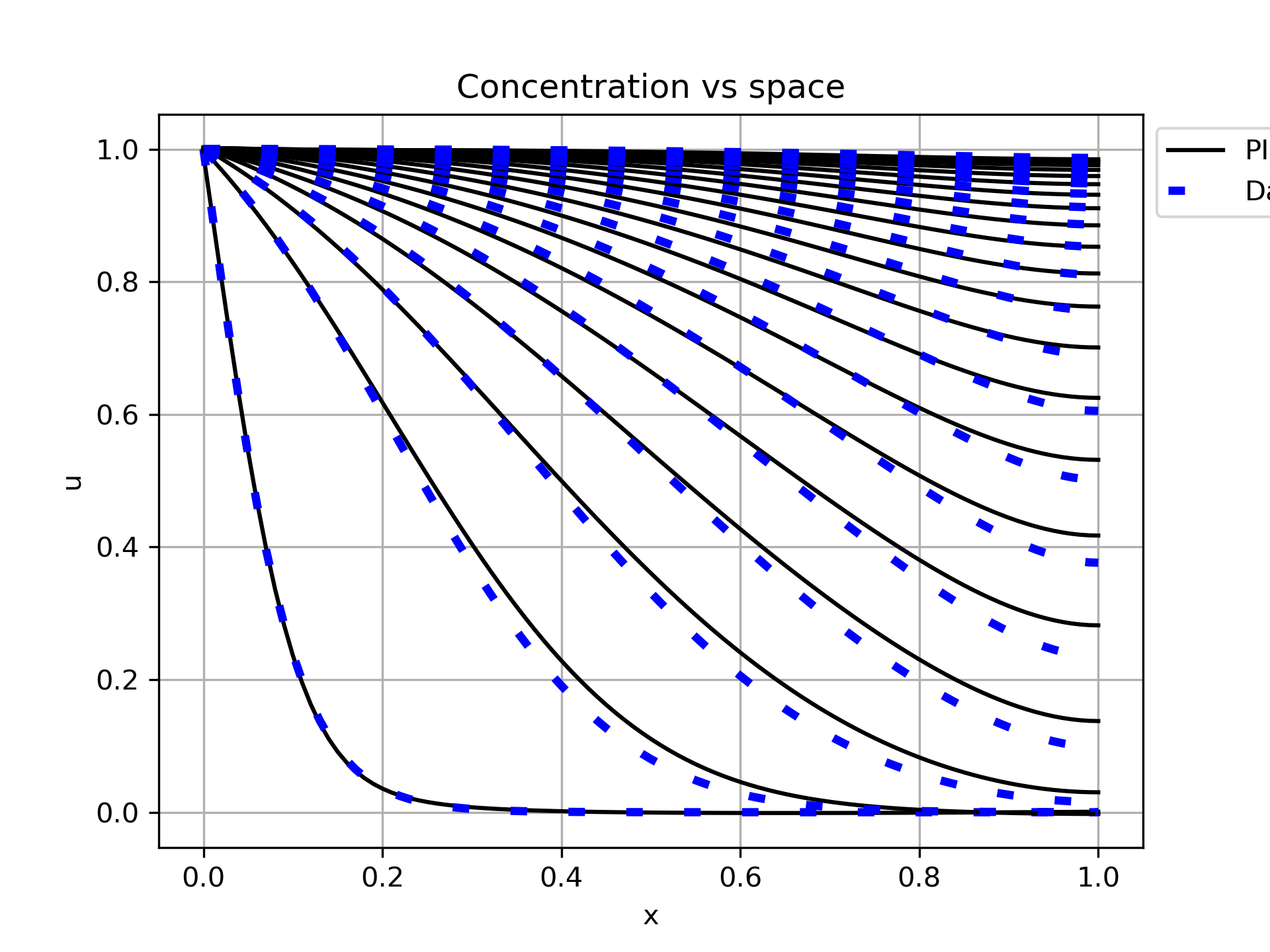
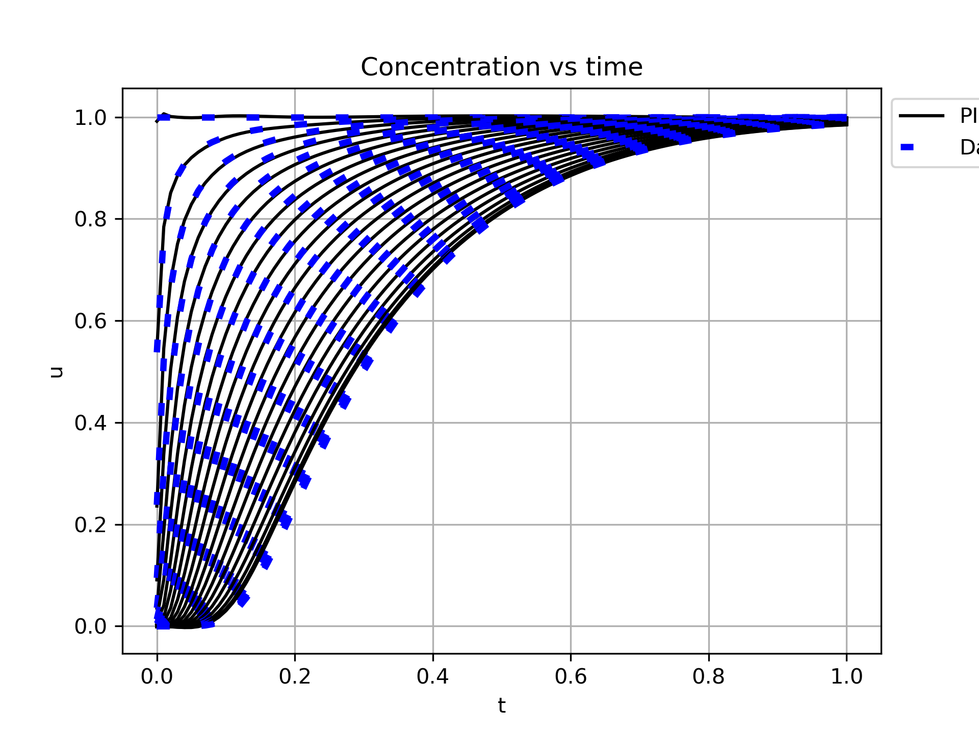
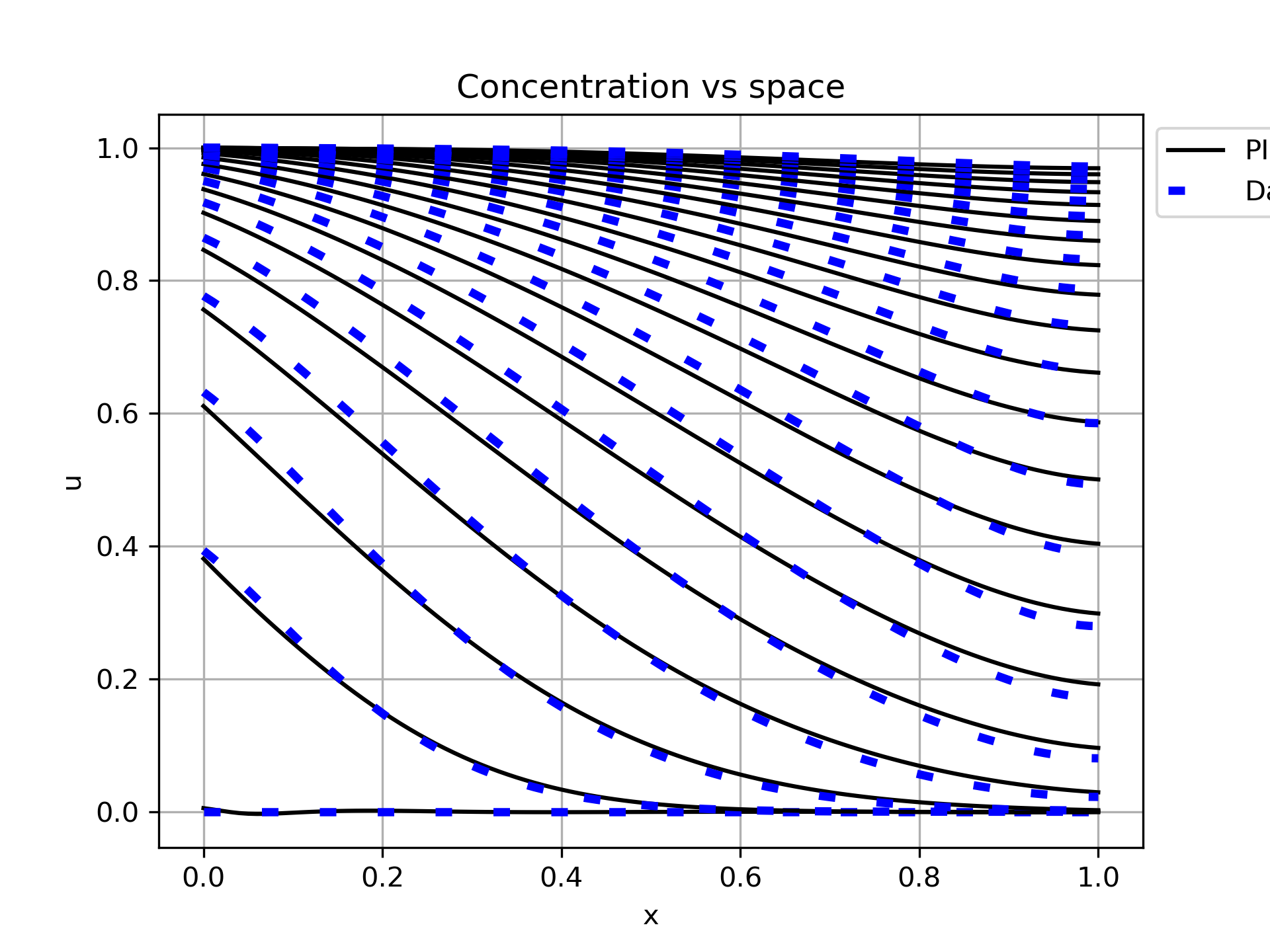
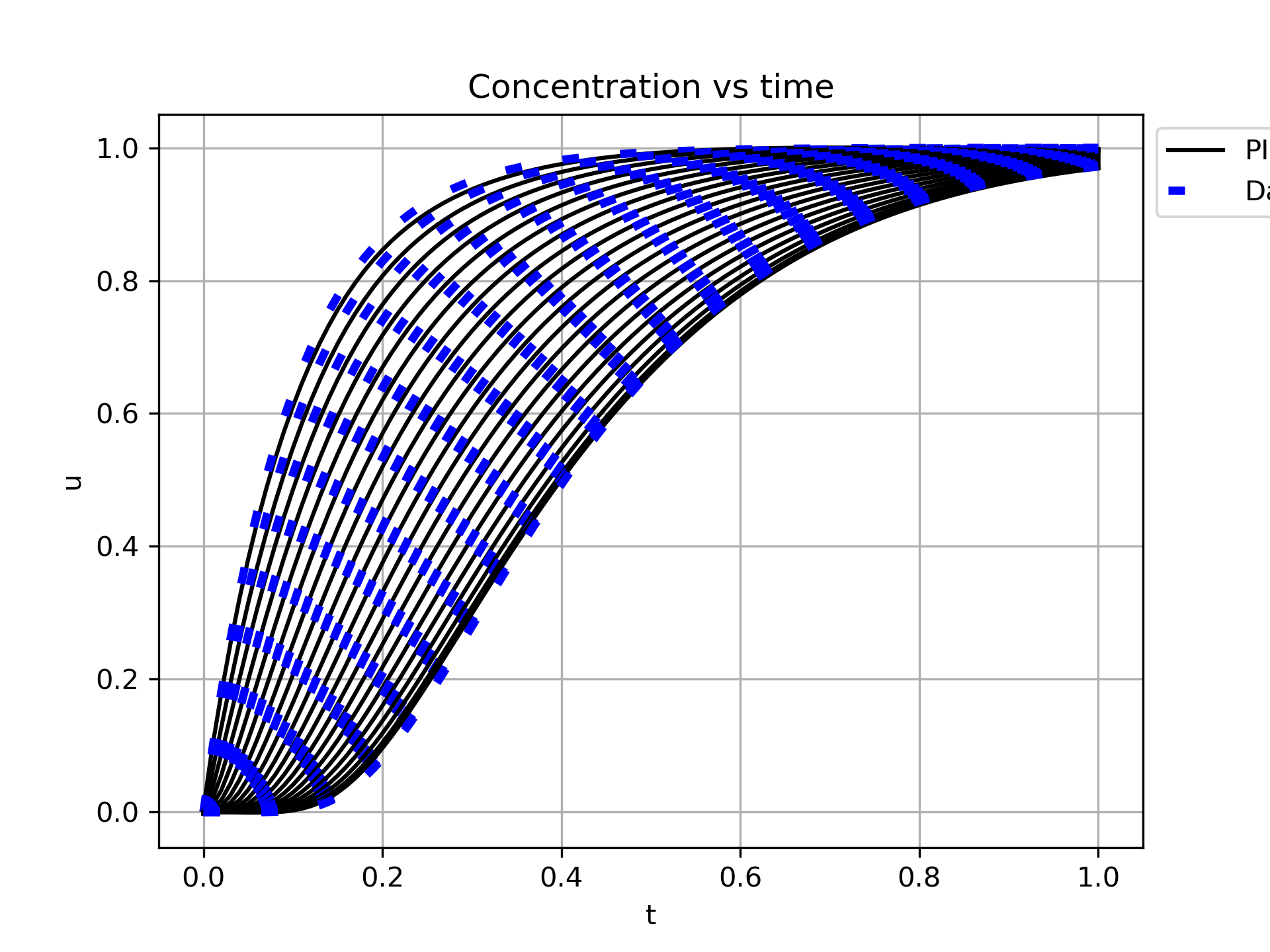
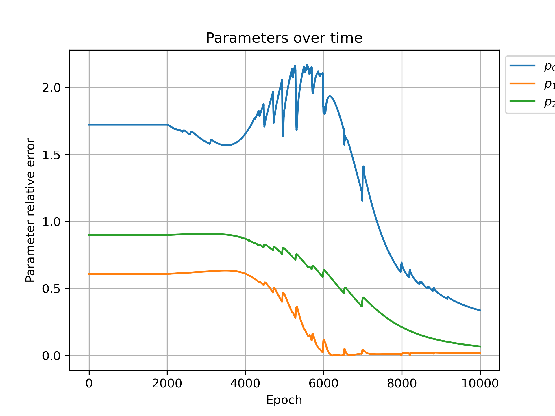
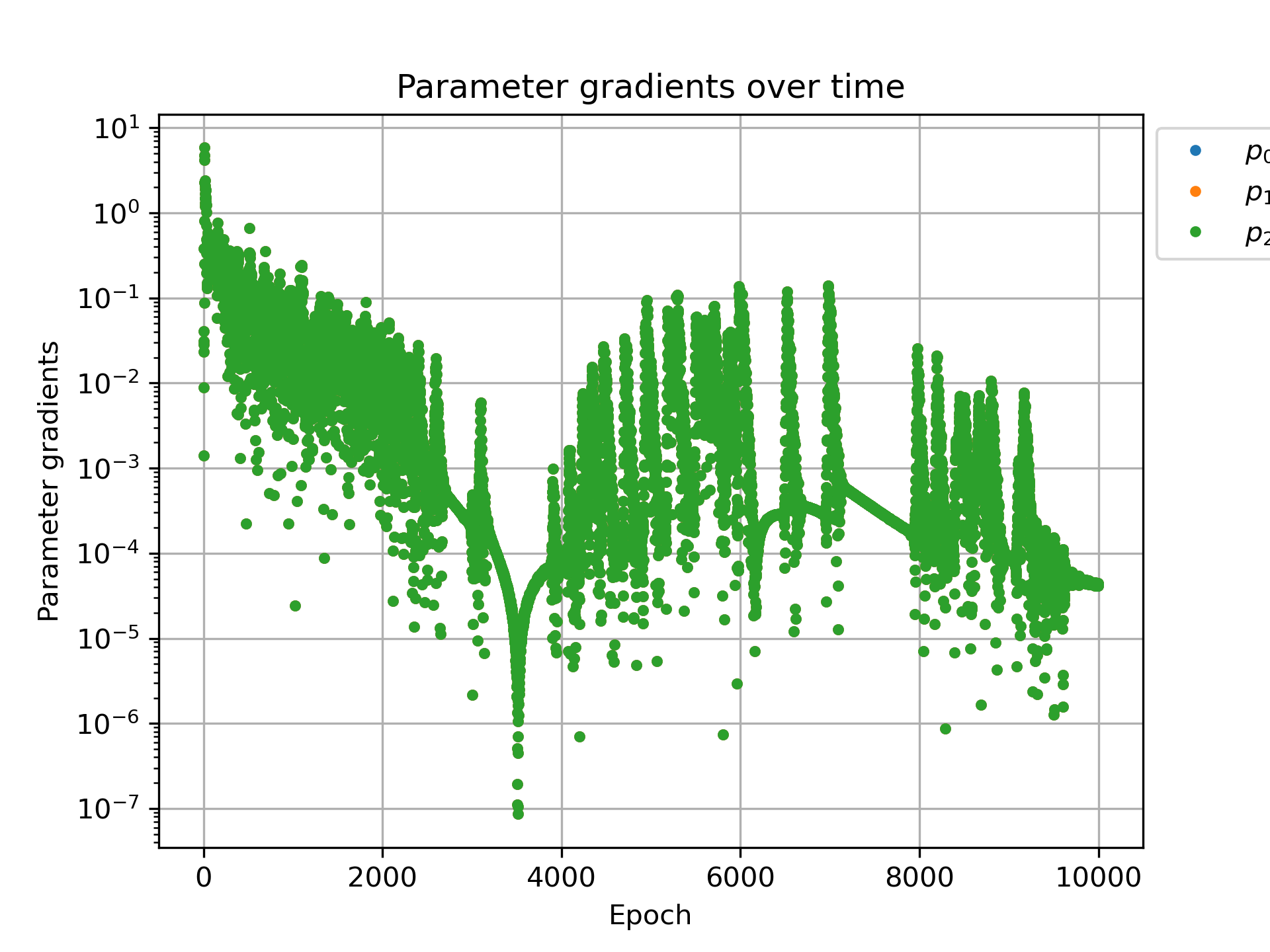
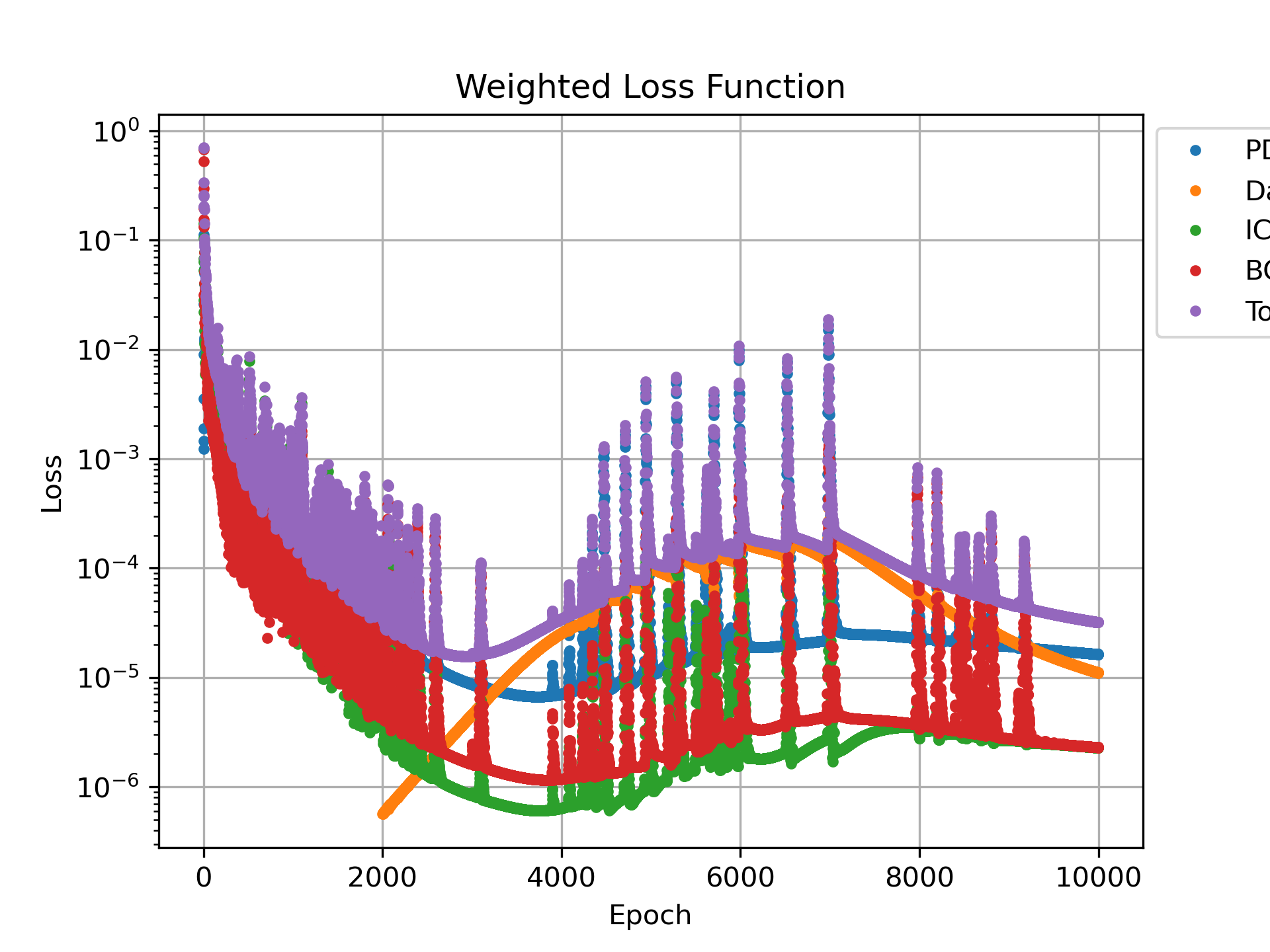
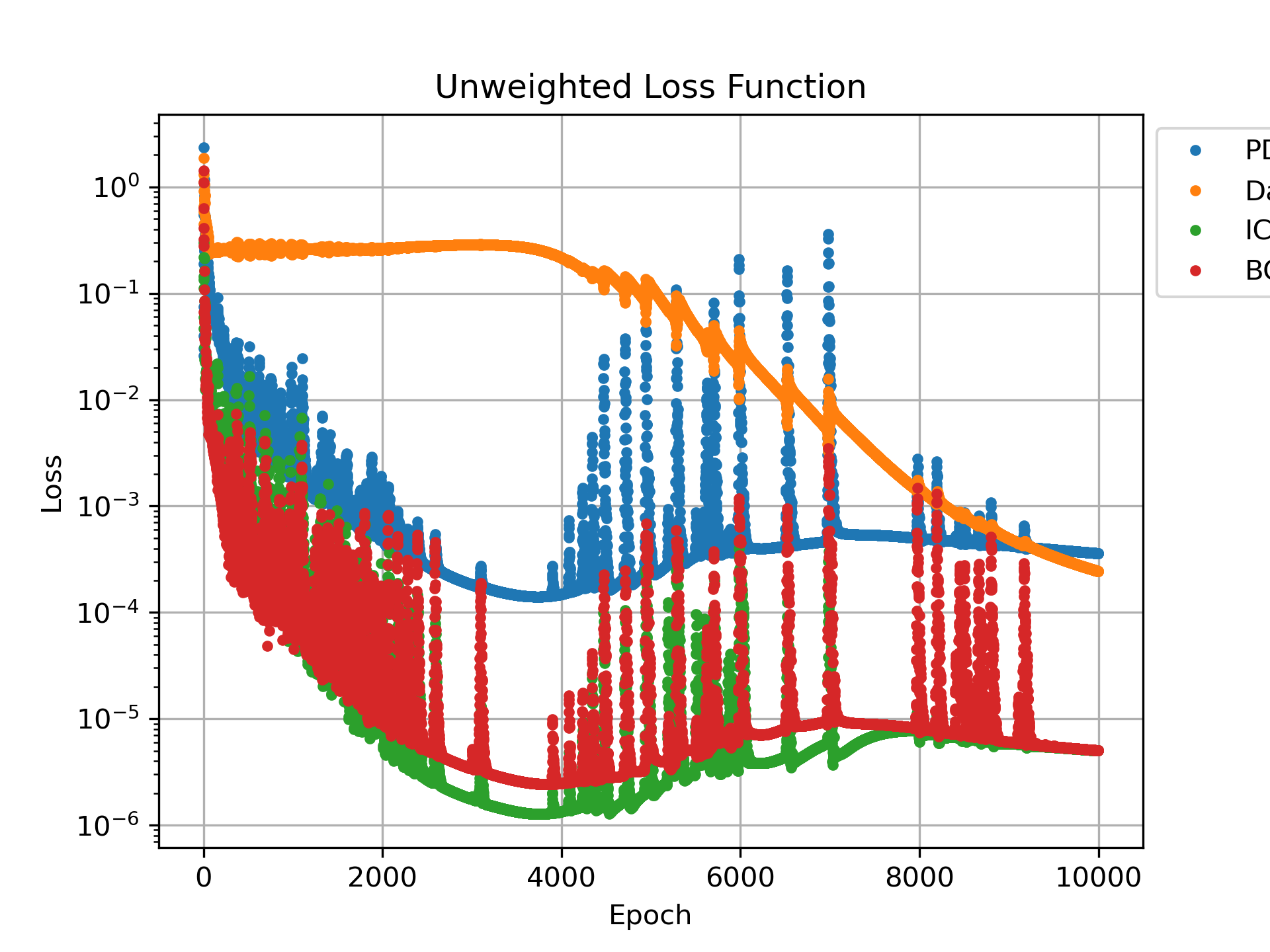
In figs. 8 and 9 we show the solution of the advection-diffusion with mobile-immobile model obtained with the PINN, for the mobile and immobile phase, respectively. The solution is compared with the reference data generated by chebfun. The solution is shown as a function of space for different times (left) and as a function of time for different space locations (right). The solution obtained with the PINN is in good agreement with the reference data, showing that the PINN is able to accurately solve the direct problem.

5 Conclusions

In this paper, we have proposed an adaptive inverse PINN architecture for solving transport problems in porous materials. These include a diffusion, advection-diffusion and mobile-immobile formulations. We propose a robust PINN architecture and training algorithm that can reproduce well the forward problem and the inverse problem for up to three parameters. Ongoing work include the extension to two-dimensional problems, larger number of parameters and non-parametric functional form of the parameteres to include heterogeneities and non-linear dependencies. The main novelty of the proposed approach is the adaptive scaling of the loss function components and gradients of the trainable parameters. This adaptive scaling is crucial for the convergence of the inverse problem, as it ensures that the different components of the loss function are balanced and that the gradients of the trainable parameters are scaled appropriately. We have demonstrated the effectiveness of the proposed approach through a series of numerical experiments, showing that the adaptive inverse PINN architecture is scalable, robust, and efficient for solving a wide range of transport models.

References

- Alebrahim [2023] R. Alebrahim. Modified wave dispersion properties in 1D and 2D state-based peridynamic media. Computers & Mathematics with Applications, 151:21–35, 2023. ISSN 0898-1221. https://doi.org/10.1016/j.camwa.2023.09.007. URL https://www.sciencedirect.com/science/article/pii/S0898122123003929.
- Alebrahim and Marfia [2023] R. Alebrahim and S. Marfia. Adaptive PD-FEM coupling method for modeling pseudo-static crack growth in orthotropic media. Engineering Fracture Mechanics, 294:109710, 2023. ISSN 0013-7944. https://doi.org/10.1016/j.engfracmech.2023.109710. URL https://www.sciencedirect.com/science/article/pii/S0013794423006689.
- Amini et al. [2022] Danial Amini, Ehsan Haghighat, and Ruben Juanes. Physics-informed neural network solution of thermo–hydro–mechanical processes in porous media. Journal of Engineering Mechanics, 148(11):04022070, 2022.
- Bandai and Ghezzehei [2022] T. Bandai and T. A. Ghezzehei. Forward and inverse modeling of water flow in unsaturated soils with discontinuous hydraulic conductivities using physics-informed neural networks with domain decomposition. Hydrology and Earth System Sciences, 26(16):4469–4495, 2022. 10.5194/hess-26-4469-2022.
- Baydin et al. [2017] Atılım Günes Baydin, Barak A. Pearlmutter, Alexey Andreyevich Radul, and Jeffrey Mark Siskind. Automatic Differentiation in Machine Learning: A Survey. J. Mach. Learn. Res., 18(1):5595–5637, jan 2017. ISSN 1532-4435.
- Behera et al. [2022] Deepak Behera, Pranesh Roy, Sundaram Vinod K. Anicode, Erdogan Madenci, and Benjamin Spencer. Imposition of local boundary conditions in peridynamics without a fictitious layer and unphysical stress concentrations. Computer Methods in Applied Mechanics and Engineering, 393:114734, 2022. ISSN 0045-7825. https://doi.org/10.1016/j.cma.2022.114734.
- Bengio et al. [2003] Yoshua Bengio, Réjean Ducharme, Pascal Vincent, and Christian Janvin. A Neural Probabilistic Language Model. Journal of Machine Learning Research, 3:1137–1155, mar 2003. ISSN 1532-4435.
- Berardi et al. [2023a] M. Berardi, F. V. Difonzo, and S. F. Pellegrino. A Numerical Method for a Nonlocal Form of Richards’ Equation Based on Peridynamic Theory. Computers & Mathematics with Applications, 143:23–32, 2023a. https://doi.org/10.1016/j.camwa.2023.04.032.
- Berardi and Girardi [2024] Marco Berardi and Giovanni Girardi. Modeling plant water deficit by a non-local root water uptake term in the unsaturated flow equation. Communications in Nonlinear Science and Numerical Simulation, 128:107583, 2024. ISSN 1007-5704. https://doi.org/10.1016/j.cnsns.2023.107583.
- Berardi et al. [2023b] Marco Berardi, Fabio V. Difonzo, and Roberto Guglielmi. A preliminary model for optimal control of moisture content in unsaturated soils. Computational Geosciences, 27(6):1133–1144, Dec 2023b. 10.1007/s10596-023-10250-1.
- Bobaru et al. [2009] F. Bobaru, M. Yang, S. Alves, F.and Silling, E. Askari, and J. Xu. Convergence, adaptive refinement, and slaning in 1D peridynamics. Int. J. Numer. Mech. Eng., 77:852 – 877, 2009. https://doi.org/10.1002/nme.2439.
- Bolte and Pauwels [2020] Jérôme Bolte and Edouard Pauwels. A mathematical model for automatic differentiation in machine learning. In H. Larochelle, M. Ranzato, R. Hadsell, M.F. Balcan, and H. Lin, editors, Advances in Neural Information Processing Systems, volume 33, pages 10809–10819. Curran Associates, Inc., 2020. URL https://proceedings.neurips.cc/paper_files/paper/2020/file/7a674153c63cff1ad7f0e261c369ab2c-Paper.pdf.
- Celia et al. [1990] Michael A. Celia, Efthimios T. Bouloutas, and Rebecca L. Zarba. A general mass-conservative numerical solution for the unsaturated flow equation. Water Resources Research, 26(7):1483–1496, 1990. ISSN 1944-7973. 10.1029/WR026i007p01483. URL http://dx.doi.org/10.1029/WR026i007p01483.
- Chen et al. [2020] Yuyao Chen, Lu Lu, George Em Karniadakis, and Luca Dal Negro. Physics-informed neural networks for inverse problems in nano-optics and metamaterials. Opt. Express, 28(8):11618–11633, Apr 2020. 10.1364/OE.384875.
- Coclite et al. [2020] G. M. Coclite, A. Fanizzi, L. Lopez, F. Maddalena, and S. F. Pellegrino. Numerical methods for the nonlocal wave equation of the peridynamics. Applied Numerical Mathematics, 155:119 – 139, 2020. ISSN 0168-9274. https://doi.org/10.1016/j.apnum.2018.11.007.
- Cuomo et al. [2022] Salvatore Cuomo, Vincenzo Schiano Di Cola, Fabio Giampaolo, Gianluigi Rozza, Maziar Raissi, and Francesco Piccialli. Scientific Machine Learning Through Physics–Informed Neural Networks: Where we are and What’s Next. Journal of Scientific Computing, 92(3):88, Jul 2022. ISSN 1573-7691. 10.1007/s10915-022-01939-z.
- Cybenko [1989] G. Cybenko. Approximation by superpositions of a sigmoidal function. Mathematics of Control, Signals and Systems, 2(4):303–314, Dec 1989. 10.1007/BF02551274. URL https://doi.org/10.1007/BF02551274.
- D’Elia and Yu [2021] Marta D’Elia and Yue Yu. On the prescription of boundary conditions for nonlocal Poisson’s and peridynamics models. arXiv preprint arXiv:2107.04450, 2021. 10.48550/ARXIV.2107.04450. URL https://arxiv.org/abs/2107.04450.
- D’Elia et al. [2022] Marta D’Elia, Hang Deng, Cedric Fraces, Krishna Garikipati, Lori Graham-Brady, Amanda Howard, George Karniadakis, Vahid Keshavarzzadeh, Robert M Kirby, Nathan Kutz, et al. Machine learning in heterogeneous porous materials. arXiv preprint arXiv:2202.04137, 2022.
- Dentz et al. [2018] Marco Dentz, Matteo Icardi, and Juan J Hidalgo. Mechanisms of dispersion in a porous medium. Journal of Fluid Mechanics, 841:851–882, 2018.
- Difonzo and Garrappa [2023] Fabio V. Difonzo and Roberto Garrappa. A Numerical Procedure for Fractional-Time-Space Differential Equations with the Spectral Fractional Laplacian. In Angelamaria Cardone, Marco Donatelli, Fabio Durastante, Roberto Garrappa, Mariarosa Mazza, and Marina Popolizio, editors, Fractional Differential Equations, pages 29–51, Singapore, 2023. Springer Nature Singapore.
- Difonzo et al. [2024] Fabio V. Difonzo, Luciano Lopez, and Sabrina F. Pellegrino. Physics informed neural networks for an inverse problem in peridynamic models. Engineering with Computers, Mar 2024. ISSN 1435-5663. 10.1007/s00366-024-01957-5.
- Gao et al. [2022] Han Gao, Matthew J. Zahr, and Jian-Xun Wang. Physics-informed graph neural Galerkin networks: A unified framework for solving PDE-governed forward and inverse problems. Computer Methods in Applied Mechanics and Engineering, 390:114502, 2022. ISSN 0045-7825. https://doi.org/10.1016/j.cma.2021.114502.
- Guo et al. [2022] Shenghan Guo, Mohit Agarwal, Clayton Cooper, Qi Tian, Robert X Gao, Weihong Guo Grace, and YB Guo. Machine learning for metal additive manufacturing: Towards a physics-informed data-driven paradigm. Journal of Manufacturing Systems, 62:145–163, 2022.
- Gusmão and Medford [2024] G.S. Gusmão and A.J. Medford. Maximum-likelihood estimators in physics-informed neural networks for high-dimensional inverse problems. Computers & Chemical Engineering, 181:108547, 2024. https://doi.org/10.1016/j.compchemeng.2023.108547.
- Haghighat et al. [2021] Ehsan Haghighat, Ali Can Bekar, Erdogan Madenci, and Ruben Juanes. A nonlocal physics-informed deep learning framework using the peridynamic differential operator. Computer Methods in Applied Mechanics and Engineering, 385:114012, 2021. ISSN 0045-7825. https://doi.org/10.1016/j.cma.2021.114012. URL https://www.sciencedirect.com/science/article/pii/S0045782521003431.
- Haghighat et al. [2022] Ehsan Haghighat, Danial Amini, and Ruben Juanes. Physics-informed neural network simulation of multiphase poroelasticity using stress-split sequential training. Computer Methods in Applied Mechanics and Engineering, 397, 2022. 10.1016/j.cma.2022.115141.
- He and Tartakovsky [2021] QiZhi He and Alexandre M Tartakovsky. Physics-informed neural network method for forward and backward advection-dispersion equations. Water Resources Research, 57(7):e2020WR029479, 2021.
- He et al. [2020] QiZhi He, David Barajas-Solano, Guzel Tartakovsky, and Alexandre M Tartakovsky. Physics-informed neural networks for multiphysics data assimilation with application to subsurface transport. Advances in Water Resources, 141:103610, 2020.
- Hornik et al. [1989] Kurt Hornik, Maxwell Stinchcombe, and Halbert White. Multilayer feedforward networks are universal approximators. Neural Networks, 2(5):359–366, 1989. ISSN 0893-6080. https://doi.org/10.1016/0893-6080(89)90020-8. URL https://www.sciencedirect.com/science/article/pii/0893608089900208.
- Ivan Depina and Gotovac [2022] Sigurdur Mar Valsson Ivan Depina, Saket Jain and Hrvoje Gotovac. Application of physics-informed neural networks to inverse problems in unsaturated groundwater flow. Georisk: Assessment and Management of Risk for Engineered Systems and Geohazards, 16(1):21–36, 2022. 10.1080/17499518.2021.1971251.
- Jeong et al. [2024] Iksu Jeong, Maenghyo Cho, Hayoung Chung, and Do-Nyun Kim. Data-driven nonparametric identification of material behavior based on physics-informed neural network with full-field data. Computer Methods in Applied Mechanics and Engineering, 418:116569, 2024.
- Karniadakis et al. [2021] George Em Karniadakis, Ioannis G Kevrekidis, Lu Lu, Paris Perdikaris, Sifan Wang, and Liu Yang. Physics-informed machine learning. Nature Reviews Physics, 3(6):422–440, 2021.
- Kilic and Madenci [2010] B. Kilic and E. Madenci. Coupling of peridynamic theory and the finite element method. Journal of Mechanics of Materials and Structures, 5(5):703 – 733, 2010. https://doi.org/10.1007/978-1-4614-8465-3_11.
- Lapidus and Amundson [1952] Leon Lapidus and Neal R Amundson. Mathematics of adsorption in beds. vi. the effect of longitudinal diffusion in ion exchange and chromatographic columns. The Journal of Physical Chemistry, 56(8):984–988, 1952.
- Lopez and Pellegrino [2021] L. Lopez and S. F. Pellegrino. A spectral method with volume penalization for a nonlinear peridynamic model. International Journal for Numerical Methods in Engineering, 122(3):707–725, 2021. https://doi.org/10.1002/nme.6555.
- Lopez and Pellegrino [2022a] L. Lopez and S. F. Pellegrino. A non-periodic Chebyshev spectral method avoiding penalization techniques for a class of nonlinear peridynamic models. International Journal for Numerical Methods in Engineering, 123(20):4859–4876, 2022a. https://doi.org/10.1002/nme.7058.
- Lopez and Pellegrino [2022b] L. Lopez and S. F. Pellegrino. A fast-convolution based space–time Chebyshev spectral method for peridynamic models. Advances in Continuous and Discrete Models, 70(1), 2022b. https://doi.org/10.1186/s13662-022-03738-0. URL https://doi.org/10.1186/s13662-022-03738-0.
- Lopez and Pellegrino [2023] Luciano Lopez and Sabrina Francesca Pellegrino. Computation of Eigenvalues for Nonlocal Models by Spectral Methods. Journal of Peridynamics and Nonlocal Modeling, 5(2):133–154, 2023. 10.1007/s42102-021-00069-8. URL https://doi.org/10.1007/s42102-021-00069-8.
- Marcato et al. [2023] Agnese Marcato, Daniele Marchisio, and Gianluca Boccardo. Reconciling deep learning and first-principle modelling for the investigation of transport phenomena in chemical engineering. The Canadian Journal of Chemical Engineering, 101(6):3013–3018, 2023.
- Masciopinto and Passarella [2018] Costantino Masciopinto and Giuseppe Passarella. Mass-transfer impact on solute mobility in porous media: A new mobile-immobile model. Journal of Contaminant Hydrology, 215:21–28, 2018. https://doi.org/10.1016/j.jconhyd.2018.06.004.
- Mavi et al. [2023] A. Mavi, A.C. Bekar, E. Haghighat, and E. Madenci. An unsupervised latent/output physics-informed convolutional-LSTM network for solving partial differential equations using peridynamic differential operator. Computer Methods in Applied Mechanics and Engineering, 407, 2023. https://doi.org/10.1016/j.cma.2023.115944.
- McClenny and Braga-Neto [2022] Levi McClenny and Ulisses Braga-Neto. Self-adaptive physics-informed neural networks using a soft attention mechanism, 2022.
- Meng et al. [2023] Zeng Meng, Qiaochu Qian, Mengqiang Xu, Bo Yu, Ali Riza Yildiz, and Seyedali Mirjalili. PINN-FORM: A new physics-informed neural network for reliability analysis with partial differential equation. Computer Methods in Applied Mechanics and Engineering, 414:116172, 2023. ISSN 0045-7825. https://doi.org/10.1016/j.cma.2023.116172.
- Municchi and Icardi [2020a] Federico Municchi and Matteo Icardi. Generalized multirate models for conjugate transfer in heterogeneous materials. Phys. Rev. Res., 2:013041, Jan 2020a. 10.1103/PhysRevResearch.2.013041. URL https://link.aps.org/doi/10.1103/PhysRevResearch.2.013041.
- Municchi and Icardi [2020b] Federico Municchi and Matteo Icardi. Generalized multirate models for conjugate transfer in heterogeneous materials. Physical Review Research, 2(1):013041, 2020b.
- Municchi et al. [2021] Federico Municchi, Nicodemo Di Pasquale, Marco Dentz, and Matteo Icardi. Heterogeneous multi-rate mass transfer models in openfoam®. Computer Physics Communications, 261:107763, 2021.
- Park et al. [2020] Sejun Park, Chulhee Yun, Jaeho Lee, and Jinwoo Shin. Minimum width for universal approximation. arXiv preprint arXiv:2006.08859, 2020.
- Pellegrino [2021] S. F. Pellegrino. Simulations on the peridynamic equation in continuum mechanics. Springer Proceedings in Complexity. 13th Chaotic Modeling and Simulation International Conference, CHAOS 2020, pages 635–649, 2021. https://doi.org/10.1007/978-3-030-70795-8_46.
- Pinkus [1999] Allan Pinkus. Approximation theory of the MLP model in neural networks. Acta Numerica, 8:143–195, 1999. 10.1017/S0962492900002919.
- Raissi et al. [2019] M. Raissi, P. Perdikaris, and G.E. Karniadakis. Physics-informed neural networks: A deep learning framework for solving forward and inverse problems involving nonlinear partial differential equations. Journal of Computational Physics, 378:686–707, 2019. ISSN 0021-9991. https://doi.org/10.1016/j.jcp.2018.10.045.
- Regazzoni et al. [2019] F. Regazzoni, L. Dedè, and A. Quarteroni. Machine learning for fast and reliable solution of time-dependent differential equations. Journal of Computational Physics, 397:108852, 2019. ISSN 0021-9991. https://doi.org/10.1016/j.jcp.2019.07.050. URL https://www.sciencedirect.com/science/article/pii/S0021999119305364.
- Santos et al. [2020] Javier E Santos, Duo Xu, Honggeun Jo, Christopher J Landry, Mavsa Prodanović, and Michael J Pyrcz. Poreflow-net: A 3d convolutional neural network to predict fluid flow through porous media. Advances in Water Resources, 138:103539, 2020.
- Sener and Koltun [2018] Ozan Sener and Vladlen Koltun. Multi-task learning as multi-objective optimization. Advances in neural information processing systems, 31, 2018.
- Shojaei et al. [2016] A. Shojaei, T. Mudric, M. Zaccariotto, and U. Galvanetto. A coupled meshless finite point/Peridynamic method for 2D dynamic fracture analysis. International Journal of Mechanical Sciences, 119:419 – 431, 2016. ISSN 0020-7403. https://doi.org/10.1016/j.ijmecsci.2016.11.003.
- Silling and Askari [2005] S. Silling and E. Askari. A meshfree based on the peridynamic model of solid mechanics. Computer & Structures, 83(17–18):1526–1535, 2005. https://doi.org/10.1016/j.compstruc.2004.11.026.
- Sukumar and Srivastava [2022] N. Sukumar and Ankit Srivastava. Exact imposition of boundary conditions with distance functions in physics-informed deep neural networks. Computer Methods in Applied Mechanics and Engineering, 389:114333, 2022. ISSN 0045-7825. https://doi.org/10.1016/j.cma.2021.114333. URL https://www.sciencedirect.com/science/article/pii/S0045782521006186.
- Taylor et al. [2023] Jamie M. Taylor, David Pardo, and Ignacio Muga. A Deep Fourier Residual method for solving PDEs using Neural Networks. Computer Methods in Applied Mechanics and Engineering, 405:115850, 2023. ISSN 0045-7825. https://doi.org/10.1016/j.cma.2022.115850. URL https://www.sciencedirect.com/science/article/pii/S0045782522008064.
- Turner et al. [2015] D.Z. Turner, B.G. van Bloemen Waanders, and M.L. Parks. Inverse problems in heterogeneous and fractured media using peridynamics. Journal of Mechanics of Materials and Structures, 10(5), 2015. https://doi.org/10.2140/jomms.2015.10.573.
- Upadhyay et al. [2024] Kshitiz Upadhyay, Jan N Fuhg, Nikolaos Bouklas, and KT Ramesh. Physics-informed data-driven discovery of constitutive models with application to strain-rate-sensitive soft materials. Computational Mechanics, pages 1–30, 2024.
- Vitullo et al. [2024] P. Vitullo, A. Colombo, N.R. Franco, A. Manzoni, and P. Zunino. Nonlinear model order reduction for problems with microstructure using mesh informed neural networks. Finite Elements in Analysis and Design, 229:104068, 2024. ISSN 0168-874X. https://doi.org/10.1016/j.finel.2023.104068. URL https://www.sciencedirect.com/science/article/pii/S0168874X23001610.
- Wang et al. [2023a] L. Wang, S. Jafarzadeh, F. Mousavi, and F. Bobaru. PeriFast/Corrosion: A 3D Pseudospectral Peridynamic MATLAB Code for Corrosion. Journal of Peridynamics and Nonlocal Modeling, pages 1–25, 2023a. https://doi.org/10.1007/s42102-023-00098-5.
- Wang et al. [2023b] Shupeng Wang, Hui Zhang, and Xiaoyun Jiang. Physics-informed neural network algorithm for solving forward and inverse problems of variable-order space-fractional advection–diffusion equations. Neurocomputing, 535:64–82, 2023b.
- Xu et al. [2023] Chen Xu, Ba Trung Cao, Yong Yuan, and Günther Meschke. Transfer learning based physics-informed neural networks for solving inverse problems in engineering structures under different loading scenarios. Computer Methods in Applied Mechanics and Engineering, 405:115852, 2023. ISSN 0045-7825. https://doi.org/10.1016/j.cma.2022.115852.
- Yang et al. [2021] Liu Yang, Xuhui Meng, and George Em Karniadakis. B-pinns: Bayesian physics-informed neural networks for forward and inverse pde problems with noisy data. Journal of Computational Physics, 425:109913, 2021. https://doi.org/10.1016/j.jcp.2020.109913.
- Yu et al. [2020] Tianhe Yu, Saurabh Kumar, Abhishek Gupta, Sergey Levine, Karol Hausman, and Chelsea Finn. Gradient surgery for multi-task learning, 2020.
- Yuan et al. [2022] L. Yuan, Y.Q. Ni, X.Y. Deng, and S. Hao. A-PINN: Auxiliary physics informed neural networks for forward and inverse problems of nonlinear integro-differential equations. Journal of Computational Physics, 462, 2022. https://doi.org/10.1016/j.jcp.2022.111260.
- Zaccariotto et al. [2018] M. Zaccariotto, T. Mudric, D. Tomasi, A. Shojaei, and U. Galvanetto. Coupling of FEM meshes with Peridynamic grids. Computer Methods in Applied Mechanics and Engineering, 330:471 – 497, 2018. https://doi.org/10.1016/j.cma.2017.11.011.
- Zhou et al. [2023] Z. Zhou, L. Wang, and Z. Yan. Deep neural networks learning forward and inverse problems of two-dimensional nonlinear wave equations with rational solitons. Computers and Mathematics with Applications, 151:164–171, 2023. https://doi.org/10.1016/j.camwa.2023.09.047.