The Dynamic, the Static, and the Weak
factor models and the analysis of high-dimensional time series
Abstract
Several fundamental and closely interconnected issues related to factor models are reviewed and discussed: dynamic versus static loadings, rate-strong versus rate-weak factors, the concept of weakly common component recently introduced by Gersing et al. (2023), the irrelevance of cross-sectional ordering and the assumption of cross-sectional exchangeability, and the problem of undetected strong factors.
Keywords: Static factor models; Dynamic factor models; Weak factors; Cross-sectional exchangeability; Undetected factors.
1 Introduction: Spearman and the origins of factor models
Factor models and factor model methods are rooted in early-twentieth-century psychometrics. It is usually admitted that the concept of factor first appears more than a century ago in Spearman (1904) where a factor model is proposed in order to account for the dependencies between several variables related with cognitive abilities measured on given individuals. The result was a two-factor theory in which cognitive performance was explained by two unobservable “factors.” The objective of these early factor models, thus, is to account for cross-sectional dependencies—more specifically, cross-sectional covariances or correlations—in an i.i.d. context.
Spearman’s exposition does not match the mathematical standards of present-day psychometrics or statistics, and more precise mathematical descriptions of factor models only came somewhat later. Classical references are, among many others, Hotelling (1933a, b), Bartlett (1937, 1938), Jöreskog (1969), or the monograph by Lawley and Maxwell (1971); see Jöreskog (2007) for a historical account.
In that i.i.d. context, a factor model with factors is a statistical model characterized by an equation of the form (the index here does not stand for time and is used to facilitate comparisons with the time-series case to be described later)
| (1.1) |
where
-
(a)
is an i.i.d. sample of -dimensional observations with (for ease of exposition and without loss of generality) and , ;
-
(b)
is an unspecified matrix of scalar loadings with row vectors , ;
-
(c)
, is an i.i.d. sample of latent (unobservable) -dimensional variables, the (common) factors, with and ; call the common component of ;
-
(d)
, is an unobserved sample from an i.i.d. process of -dimensional variables with and diagonal; call the idiosyncratic component of ;
-
(e)
the factors and the idiosyncratic component (hence also the common and the idiosyncratic components) are mutually orthogonal: , , , and
Equation (1.1) thus decomposes the component of the observation into two unobservable and mutually orthogonal components: the common component and the idiosyncratic component . All subsequent factor models are based on such a decomposition, with various restrictions on and : call it the factor model decomposition. Because the idiosyncratic in (1.1) is a vector of mutually orthogonal white noises, this traditional model is called an exact factor model. The nature of (1.1), along with assumptions (a)–(e), is that of a semiparametric statistical model with parameters the loadings and nuisances the unspecified distributions of and .
Estimation of this exact static factor model is typically performed via Gaussian MLE, which gives consistent estimates only for the loadings as , while the factors (which can be treated as incidental parameters) cannot be consistently estimated since is fixed (Anderson and Rubin, 1956; Lawley and Maxwell, 1971; Amemiya et al., 1987). The MLE, moreover, also requires finite 4th order moments of the observables.
The observations in (1.1) being i.i.d., this exact model is of limited interest in the analysis of econometric data, where serial dependence is ubiquitous. The development of factor models in time-series and econometrics only began in the late seventies with the dynamic exact factor models of Geweke (1977) and Sargent and Sims (1977), who allow for factor-induced serial dependence and, a few years later, with the static approximate factor model of Chamberlain (1983) and Chamberlain and Rothschild (1983), who for the first time consider high-dimensional asymptotics (with both and tending to infinity) in the context.
The Chamberlain and Rothschild approach has been popularized at the turn of the century thanks to the contributions of Stock and Watson (2002a, b), Bai and Ng (2002), Bai (2003), and many others. Few years earlier Forni et al. (2000) and Forni and Lippi (2001) had introduced the Generalized or General Dynamic Factor Model (GDFM) which nests all other factor models. The static model of Chamberlain and Rothschild, however, by far remain the most popular form of factor models in econometrics.
In Section 2 we review the static approximate factor model of Chamberlain (1983) and Chamberlain and Rothschild (1983). Section 3 deals with the GDFM and, in particular, revisits Hallin and Lippi (2013) by showing that the GDFM decomposition is actually a representation result rather than just a statistical model. In Section 4 we reconsider the static approach of Chamberlain and Rothschild and show that, although less general, it can also be derived as a representation result; the proofs are developed in the Appendix. In Section 5 we discuss different concepts of weak factors, both static and dynamic. In 6 we show, both empirically and theoretically, that weak factors, in the usual acception of rate-weak factors, are incompatible with the a assumption of cross-sectional exchangeability. Section 7 discusses the crucial role of idiosyncratic components in relation to undetected factors. In Section 8 we conclude.
2 The Static: Chamberlain and Rothschild
The factor model decomposition proposed by Chamberlain (1983) and Chamberlain and Rothschild (1983) with the objective of analizing high-dimensional financial time series reads
| (2.1) |
At first sight, this decomposition into common and idiosyncratic component looks pretty much the same as the classical one (1.1). A fundamental difference, however, is that
-
(i)
the observations and the factors are no longer i.i.d.;
-
(ii)
the idiosyncratic components , are no longer i.i.d. white noise, and
-
(iii)
their covariance matrix needs not be diagonal.
Equation (2.1), thus, allows for serial dependencies among the ’s, hence for the analysisof -dimensional time series.
Since is no longer white noise and can be (serially and cross-sectionally) correlated, the model is called an approximate factor model (as opposed to the exact ones). As a consequence, it is not identified for fixed , even under the classical identification constraints. This motivates another crucial novelty: high-dimensional asymptotics are considered, with both and going to infinity, where yields asymptotic identification and allows for consistent estimation as in the classical case. The loadings, however, remain static as in (1.1).
Assumptions are quite mild:
-
(a)
is the observed finite- realization of , a second-order stationary process with (for ease of exposition and without loss of generality) and , , ;
-
(b)
is an unspecified matrix of scalar loadings with row vectors , ;
-
(c)
is the unobserved finite- realization of a second-order stationary -dimensional process of factors, with , and ;
-
(d)
letting , (the statically common component) is the value at time of the unobserved finite- realization of a latent second-order stationary process
denoting by its lag-zero covariance matrix (which has rank ), the nonzero eigenvalues of tend to infinity as ;
-
(e)
(the statically idiosyncratic component) is the value at time of the unobserved finite- realization of a second-order stationary process
with mean zero and lag-zero covariance matrix ; as , the eigenvalues of remain bounded;
-
(f)
the factors and the idiosyncratic component (hence also the common and the idiosyncratic components) are mutually orthogonal: , , , and
This static approximate factor model, like the exact model (1.1), constitutes a semiparametric statistical model, with parameters the loadings , and nuisance the unspecified distributions of the idiosyncratic process and the factors. Most people interpret the decomposition (2.1) (including the particular form of the common) as describing a data-generating process, which is irrelevant from a statistical perspective. Some (e.g. Onatski, 2012, Bai and Li, 2016) even treat the values of the factors as parameters.
Chamberlain and Rothschild do not consider the estimation problem for their approximate static factor model. Nor do they impose any rate on the divergence, as , of the eigenvalues of the covariance matrix , which in principle can be sublinear, linear, or superlinear.
Estimation is considered in Stock and Watson (2002a), Bai (2003), and Forni et al. (2009), among many others, who provide a rigorous treatment of the asymptotic properties of PCA-based estimators for the loadings and the factors of the Chamberlain and Rothschild model and show that, as expected, as both and tend to infinity, consistency (up to orthogonal transformations, as usual) is achieved for the factors and the loadings. Finite fourth-order moments of the observables are also required. QMLE methods also have been considered under the same set of assumptions (Doz et al., 2012; Bai and Li, 2016; Barigozzi and Luciani, 2024).
Typically, once factors are extracted (or estimated, with a slight abuse of language when they are not parameters) from an -dimensional ( large) time series observed over , they are used in a second step to predict a given set of target variables (Stock and Watson, 2002a, b; Bai and Ng, 2006). This approach, in general, offers sizeable improvements over univariate or small- forecasting models and, to this day, this static approximate factor model remains one of the most popular tools in the analysis of high-dimensional time series.
3 The Dynamic: Forni, Hallin, Lippi, and Reichlin
Before presenting the General Dynamic Factor Model proposed by Forni et al. (2000) and Forni and Lippi (2001), let us consider the dynamic exact factor model of Geweke (1977) and Sargent and Sims (1977), where the idea of dynamic loadings appears for the first time.
3.1 A forerunner: the dynamic exact factor model of Geweke, Sargent, and Sims
Five years before Chamberlain and Rothschild, Geweke (1977) and Sargent and Sims (1977) had understood that, if factor models were to be used in econometrics, the time-series nature of econometric data could not be ignored. A major novelty in their approach is based on the observation that factors, in economic time series, cannot be expected to be loaded simultaneously by all components of : typically, some components will load before some others. Their model accordingly considers dynamic loadings, where the row vectors of scalar loadings are replaced with row vectors of linear filters with square-summable coefficients, yielding a dynamic exact factor model: Geweke (1977)’s factor model decomposition takes the form
| (3.1) |
This idea of considering dynamic loadings was extremely innovative. On the other hand, Geweke, Sargent, and Sims do not go all the way with taking into account the time-series nature of the data, as they still assume an exact factor model, with i.i.d. and mutually orthogonal idiosyncratic components. This is a terribly strong assumption, which cannot be expected to hold in most econometric datasets. However, thanks to that assumption, their model is identified (up to an orthogonal transformation of the factors) and traditional fixed- asymptotics can be considered. The scope of their dynamic but exact factor model, thus, is not high-dimensional. Finally, just as in Chamberlain and Rothschild, their approach is a semiparametric statistical modeling one.
Variants of this dynamic exact approach have been proposed by several authors, among which Engle and Watson (1981), Shumway and Stoffer (1982), Watson and Engle (1983), and Quah and Sargent (1993), who develop a “state-space approach” where dynamics are introduced by adding a parametric dynamic equation (typically, a VAR specification) for the factors to the static factor model decomposition (2.1). A high-dimensional generalization of the latter approach was proposed by Doz et al. (2011, 2012), but we do not discuss it here.
3.2 The General Dynamic Factor Model
The General Dynamic Factor Model (henceforth GDFM) proposed by Forni et al. (2000) and Forni and Lippi (2001) is combining the dynamic loadings ideas of the exact factor model of Geweke (1977) and Sargent and Sims (1977) with the flexibility of the approximate factor model of Chamberlain (1983) and Chamberlain and Rothschild (1983). The following presentation of the GDFM is inspired from the time-domain exposition of Hallin and Lippi (2013) and slightly differs from the original ones in Forni et al. (2000) and Forni and Lippi (2001). By avoiding the spectral-domain approach, it also avoids the assumption that a spectrum exists and the possibility of spectral eigenvalues diverging only on a subset of the frequency domain.
Differently from the previous ones in Sections 2 and 3.1, the approach adopted here is purely nonparametric (as opposed to semiparametric). The only fundamental assumption we need for the existence of the GDFM factor model decomposition (3.3) is that the observation, an panel, is the finite realization, for and ( and “large”), of some double-indexed second-order time-stationary stochastic process
| (3.2) |
with (for convenience) mean zero: , , .
Instead of being part of the model specification and imposing constraints on the data-generating process, the factor model decomposition (3.3) (see below) into common and idiosyncratic is canonical and “endogenous” one, in the sense that any second-order time-stationary process of the form (3.2) determines such a decomposition; and, when additional conditions are imposed, they only involve the distribution of the observations (typically, their spectral density eigenvalues). This is in sharp contrast with the previous approaches by Chamberlain and Rothschild and Geweke, Sargent, and Sims, where the factor model decompositions (2.1) and (3.1) are part of the assumptions, along with conditions on their elements (typically, on the eigenvalues of the common and idiosyncratic covariance matrices and ).
Denote by the Hilbert space spanned by , equipped with the L2 covariance scalar product, that is, the set of all L2-convergent linear combinations of ’s () and limits of L2-convergent sequences thereof.
Definition 1.
A random variable with values in and variance is called dynamically common if either (hence a.s.) or and is the limit in quadratic mean, as , of a sequence of standardized elements of of the form , where
and is such that .
Note that the condition for all in this definition can be replacedwith , , for some constants and .
Definition 2.
Call dynamically common space of the Hilbert space spanned by the collection of all dynamically common variables in ; call dynamically idiosyncratic space its orthogonal complement (with respect to ) .
The spaces and always exist and are unique (one of them may reduce to , in which case the other ones coincides with ); in particular, they do not depend on . Intuitively, is the Hilbert space spanned by the exploding (as ) normed linear combinations, for and , of the ’s, and the limits of convergent sequences thereof.
Projecting each onto and its orthogonal complement yields the canonical decomposition
| (3.3) |
of into a dynamically common component and a dynamically idiosyncratic component , respectively, which by construction are mutually orthogonal at all leads and lags—more precisely, and are mutually orthogonal for all , and .
Call (3.3) the General Dynamic Factor (GDFM) decomposition of . Contrary to (1.1) and (2.1), this decomposition is not imposed on the data; it is canonical, always exists, and (beyond second-order stationarity) does not impose any restriction on the data-generating process of . In that sense, it is not a statistical model involving parameters, and is based on a canonical representation result. Whether that representation result is describing a data-generating process or not is irrelevant from a statistical perspective.
This nature of (3.3) as a representation result was first emphasized in Forni et al. (2000) and Forni and Lippi (2001) where, however, an additional frequency domain assumption (requiring the existence of a spectrum satisfying (3.4) below) is imposed. So far, indeed, no assumption has been imposed on the second-order stationary process . Adding the requirement that, for any , admits an spectral density matrix
( the imaginary root of -1) with eigenvalues
such that
| (3.4) |
for some finite independent of , it can be shown (Forni and Lippi, 2001; Hallin and Lippi, 2013) that the common component process is driven by a -dimensional orthonormal white noise process of common shocks. The GDFM decomposition (3.3), in that case, takes the form
| (3.5) |
for some collection of linear square-summable filters , for all ; then is the standardized innovations of . These filters (for ), moreover, can be expressed in terms of the eigenvalues and eigenvectors of . As a consequence, the GDFM decomposition (3.5) is identified.
Under assumption (3.4), the dynamically common space of , moreover, is spanned by the values (at any time ) of the first dynamic principal components , of (see Brillinger (1981) or Hallin et al. (2018) for definitions). These dynamic principal components and their empirical counterparts play, in the GDFM and its estimation method as proposed in Forni et al. (2000), a role similar to that of traditional principal components in the static factor model (2.1) of Chamberlain (1983) and Chamberlain and Rothschild (1983) and its estimation as proposed in Stock and Watson (2002a), Bai (2003), etc. Being based on spectral density matrices, this technique requires finite moments of order four, the existence of a spectrum, and the existence of an integer such that (3.4) holds; note, however, that these assumptions, contrary to the assumptions (d) and (e) underlying (2.1), only involve the observable process . That technique, unfortunately, involves two-sided filters, hence performs poorly at the ends of the observation period—making it unsuitable in a forecasting context. An alternative estimation method involving only one-sided filters is studied in Forni et al. (2015), Forni et al. (2017), and Barigozzi et al. (2024).
It is important to stress that neither Forni and Lippi (2001) nor Hallin and Lippi (2013) impose any rate on the divergence, as , of the eigenvalues of the spectral density matrix . Indeed, no divergence rate assumption is needed for identifying the model as long as a diverging gap exists between the exploding and bounded eigenvalues. When turning to estimation, Forni et al. (2000) still do not impose any rates and, because of this, cannot establish any consistency rates—on this latter issue, see Forni et al. (2004). Hallin and Liška (2007), Forni et al. (2017), and, in a more general context nesting the GDFM, Barigozzi et al. (2023), require the additional assumption of linear divergence rates, thus deriving also consistency rates for the estimators defined therein. This issue is discussed in Section 5.
4 The Approximate Static Factor Model revisited
Paralleling the characterization (3.3) of the GDFM in the previous section, a representation-based characterization of the approximate static factor decomposition of Chamberlain and Rothschild also can be obtained, which extends (2.1).
Denoting by the Hilbert space spanned by , consider the following decomposition of into a statically (at time ) common subspace and its orthogonal complement (at time and within ) .
Definition 3.
A random variable with values in and variance is called statically common at time if either (hence a.s.) or and is the limit in quadratic mean, as , of a sequence of standardized elements of of the form , where
| (4.1) |
is such that is such that .
Note that the condition for all in this definition can be replacedwith , , for some constants and .
Definition 4.
Call statically common space of at time the Hilbert space spanned by the collection of all statically common (at time ) variables in ; call statically idiosyncratic space of at time its orthogonal complement (with respect to ) .
The spaces and always exist and are unique for all . Intuitively, is the Hilbert space generated by the exploding (as ) normed linear combinations of the ’s, , for given . Contrary to its dynamic counterpart, it does depend on . It readily follows from the definitions that, for all , .
We then have the canonical decomposition
| (4.2) |
where and are the projections of on and , respectively. Orthogonality between the common and the idiosyncratic components and , however, only holds at time —more precisely, and are mutually orthogonal for all , and —while for and in (3.5) orthogonality of and holds for all , , and .
So far, (4.2) still is more general than (2.1). Adding the requirement that the eigenvalues
of the covariance matrices of (which, in view of second-order stationarity, does not depend on ) are such that
| (4.3) |
for some finite independent of , it can be shown (see the Appendix) that admits -dimensional orthonormal bases , any of which can be interpreted as an -tuple of factors, yielding a Chamberlain and Rothschild approximate static factor decomposition (2.1) satisfying the assumptions (a)–(g) of Section 2.1, with statically common component of the form . This result is new to the literature and makes the static approximate factor model decomposition also a representation result rather than a statistical model.
Note that, due to second-order stationarity, and despite the fact that , , and depend on , , its eigenvalues and eigenvectors do not; accordingly, the number of diverging eigenvalues in (4.3) (which, under (4.3), is the number of factors and the dimension of ), their values and the corresponding eigenvectors, and the projection operators and from to and (which only depend on ), are the same for all .
Finally, it is important to notice that Chamberlain and Rothschild (1983) do not impose any rate on the divergence, as , of the eigenvalues of the covariance matrix , which in principle can be sublinear, linear, or superlinear. Indeed, no divergence rate assumption is needed for identifying the model as long as an eigen-gap widening as , exists. When turning to estimation all works mentioned above make the additional assumption of a linear rate of divergence of the eigenvalues of the covariance matrix (Stock and Watson, 2002a, Bai, 2003, Forni et al., 2009, etc.). The same linear divergence assumption is made by Bai and Ng (2002) when proposing an information criterion to determine based on the behavior of sample eigenvalues.
5 The Weak: De Mol, Giannone, and Reichlin, Onatski, Hallin and Liška, and Gersing, Rust, and Deistler
The concept of weak factors appears in various places in the literature with, however, quite diverse meanings.
-
(a1)
Statically rate-weak factors in the approximate static factor model are introduced by De Mol et al. (2008) and Onatski (2012). They are related with the eigenvalues , , of the common component covariance matrix which are diverging at sublinear rates, usually parametrized as with . This is the most popular setting, see Lam and Yao (2012), Freyaldenhoven (2022), Uematsu and Yamagata (2022), and Bai and Ng (2023), among many others.
-
(a2)
Dynamically rate-weak factors in the GDFM are considered by Barigozzi and Farnè (2024) who proposed an estimator of a low-rank plus sparse spectral density matrix, under the assumption that the low-rank component has eigenvalues , , diverging at sublinear rates with , .
-
(b)
Block-specific factors are introduced by Hallin and Liška (2011), under a GDFM approach, in the context of panels divided into subpanels or blocks. The terminology weakly common factors is used for dynamic factors that are dynamically common in some block(s) but dynamically idiosyncratic in some other(s). The associated spectral eigenvalues are assumed to be diverging with the dimension of the block but no rate is specified. Approximate static factor models with a hierarchical block structure are considered, for example, by Moench et al. (2013) but without any explicit mention of weak factors.
-
(c)
Finally, Gersing et al. (2023) define weakly common components as the difference (at time ) between the dynamically common and the statically common components of . Any (possibly infinite-dimensional) orthonormal basis of the space they are spanning (at time ) then can be considered a basis of weak factors at time call them GRD-weak factors. This notion of weakness bears no relation to (a) and (b) above.
5.1 Rate-weak factors: De Mol, Giannone and Reichlin, Onatski
Following De Mol et al. (2008) and Onatski (2012), we will call a static or dynamic factor “rate-weak” or “weakly influential” if the corresponding loadings, as , are too small, or too sparse, for the corresponding eigenvalues to diverge at rate .
As mentioned in the previous sections, as long as we have a widening, as , of the eigen-gap between the first or eigenvalues of the spectral density or covariance matrix of the observables and the remaining or ones, the GDFM or the approximate static factor models are identified. Thus, for identification purposes, there is no need to assume any specific divergence rate for the divergent eigenvalues.
However, in estimation, either via dynamic or static PCA, it is often assumed that eigenvalues diverge linearly. Under this assumption, the consistency rates for the estimated common components derived in the literature always involve two terms: the first one is the classical term related to estimation of the covariance or the spectrum (in this latter case, the rate also depends on the chosen bandwidth), the second one is related to the identification of the model, and thus to the rate of divergence of the eigengap, which under linear divergence yields a rate which is . Inspection of the proofs easily shows that if the divergence rate were superlinear, consistency simply would be achieved at a faster rate.
Conversely, if the divergence were sublinear—rate , say, with —consistent estimation becomes non-trivial. Indeed, as shown by Freyaldenhoven (2022) in the static case, PCA only allows us to recover the factors which are associated with eigenvalues with divergence rate a least equal to , i.e., rate with (see also Onatski, 2012 and recent work by Fan et al., 2024). A similar result can be easily derived for dynamic PCA.
As we shall argue in Section 6, however, nonlinear growth rates, whether for static or for dynamic eigenvalues, are incompatible with the principle of irrelevant cross-sectional ordering. The question is then: for which kind of data is cross-sectional ordering relevant and thus compatible with rate-weak factors? We refer to Freyaldenhoven (2022) for a list of examples, while here we just notice that they almost all fall into the category of data having an intrinsic block structure. Such block structure can be either (1) known a priori, or (2) unknown. Case (1) is discussed in the next section. We do not discuss case (2) here, since it resembles case (1) for most aspects but estimation: the block structure being latent, indeed, classical PCA no longer applies and alternative approaches are required, see, e.g., Ando and Bai (2017).
5.2 Weak factors in panels with block structure: Hallin and Liška
Consider a panel with a blocks—namely, an panel divided into subpanels with ; for asymptotics, assume that all ’s tend to infinity as .
In a GDFM context, Hallin and Liška (2011) show that the Hilbert space then decomposes into a direct sum involving a strongly common subspace spanned by factors which are common for each -dimensional subpanel, plus mutually orthogonal weakly common subspaces spanned by factors which are common for a -tuple of subpanels but idiosyncratic for the other ones. Strongly and weakly common, here, is not related to any divergence rate, and should be understood as “strongly/weakly common in the Hallin-Liška sense". That decomposition is a refinement of the global dynamic factor model decomposition (3.5).
Hallin and Liška do not discuss rate-strength issues, but such issues naturally enter into the picture when the relative magnitudes of the block sizes exhibit different asymptotic behaviors. It is easy to see that that a given block may contain factors that are rate-strong within the block (yielding -linear divergence rate), but globally rate-weak (with -sublinear divergence rate). This happens if, for instance, that factor is idiosyncratic in all other blocks and as . There is little reason, however, to assume that for some block , as this choice of an asymptotic scenario belongs to the analyst (the observation provides no information on the asymptotic behavior of ). The objective of that choice is a good asymptotic approximation of the actual, finite- situation, and the actual value of is likely to provide a better approximation than an asymptotic value arbitrarily set to zero.
A similar approach could be taken, mutatis mutandis, with similar comments, in the context of approximate static factor models, yielding a refinement of the static factor model decomposition (2.1).
5.3 Weak factors are everywhere: Gersing, Rust, and Deistler
Under the intriguing title “Weak factors are everywhere,” Gersing et al. (2023), with the objective of reconciling the Static and the Dynamic factors, show (their approach slightly differs from the one developed here) that the statically common space , for any , is a subspace of the dynamically common one and call weakly common at time the elements of the difference : we shall call them GRD-weak.
This result naturally yields a new canonical factor decomposition, of the form
| (5.1) | ||||
where —the GRD-weakly common component of —is the difference between the dynamically and statically common components and of . This is a very ingenious idea, which shows how the GDFM (as defined in (3.5)) is overarching the static model (as defined in (2.1)) and, with the additional assumption (4.3), strictly nests the popular static model of Chamberlain (1983) and Chamberlain and Rothschild (1983). In both cases, the dynamically common space incorporates the GRD-weakly common components which, in the static approach are idiosyncratic, which explains the empirical finding (Forni et al., 2018) that the GDFM performs better in terms, e.g., of forecasting, than the static model (2.1) of Chamberlain and Rothschild even when the assumptions of the latter are satisfied.
In this new canonical decomposition (5.1), being in the dynamically common space , is orthogonal, at all leads and lags, to the dynamically idiosyncratic component ; being in the statically idiosyncratic space at time , it is also orthogonal to the statically common component at time (but not its leads and lags); that might even be a.s. zero (yielding a statically purely idiosyncratic process). Therefore, it cannot be a static factor, neither rate-strong nor rate-weak, and consists of non-pervasive lagged values of the (rate-weak or rate-strong) dynamic factors (lag-zero values included), or combinations thereof. This concept of GRD-weakly common component, thus is unrelated to the concepts of rate-weak factors discussed above.
6 Exchangeability: weak factors are nowhere!
When no block structure is present in the data, one may wonder whether the concept of rate-weak factors is really relevant in practice. An all too often overlooked feature of panel data, indeed, is that, unlike time-ordering, their cross-sectional ordering is entirely arbitrary. Very often, some alphabetical ordering is adopted, a choice that should not have any impact on the analysis. An observed panel, actually, should be treated as the equivalence class of its cross-sectional permutations. In this section we consider for simplicity of notation only the static case. The same arguments can be made verbatim for the dynamic case at the price of heavier notation.
6.1 Factors and cross-sectional permutations: intuition
To start with, let us conduct a few numerical exercises to show how cross-sectional ordering is related to the growth of eigenvalues, hence their divergence rates. First, we consider a panel generated from the very simple static one-factor model
| (6.1) |
where and , , are mutually orthogonal unit variance white noise processes, and the -dimensional column vector of loadings is of the form , with , , and , with a column vector of ones and scaled such that . Here and , hence , , and are -dimensional.
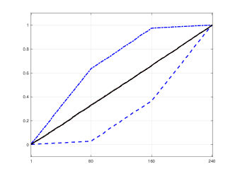
The left-hand plot in Figure 1 shows the evolution, for increasing , of the first eigenvalue (normalized by ) of the lag-zero covariance matrix in the case of three cross-sectional permutations of the ’s. Let , denote the th order statistic of the loadings: . The first permutation (dashed line) is ordering the cross-sectional items by increasing values of the loadings (); the second permutation (dashed-dotted line) orders them by decreasing values (); the third one (solid line) is alternating small and large values of the same ( for even ). From a naïve point of view, one would be tempted by a superlinear extrapolation in the first case (hence, a rate-superstrong factor) and a sublinear one (a rate-weak factor) in the second case, whereas a linear extrapolation (a rate-strong factor) looks quite reasonable in the third case. The three cases, however, are dealing with the same panel!
Second, we consider a panel generated from the static one-factor model
| (6.2) |
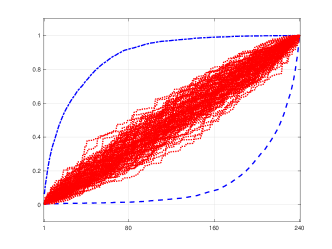
where , , and are generated as in (6.1), and , . In the right-panel of Figure 1 we show the evolution for increasing of the first eigenvalue (normalized by ) of under the following permutations. First (dashed line), when ordering the cross-section by increasing absolute values of the loadings. Second (dotted-dashed line), when ordering the cross-section by decreasing absolute values of the loadings. Third, when considering 100 random permutations of the cross-sectional units (dotted lines). In the latter case, we see that the evolution of the eigenvalue is always well described by a linear divergence in .
| deterministic cross-sectional orderings | random cross-sectional orderings |
 |
 |
 |
 |
Third, we consider the same exercise but for a two-factor model
| (6.3) |
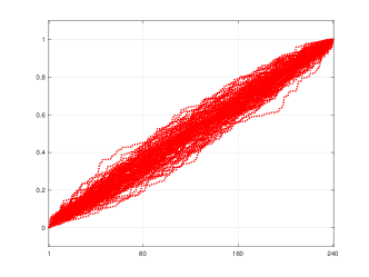
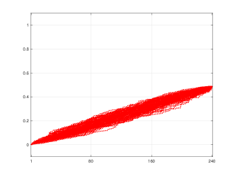
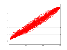
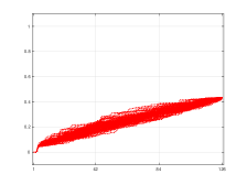
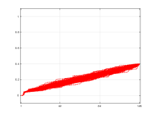
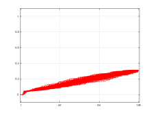
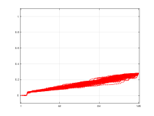
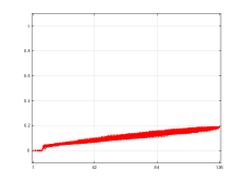
where , , and , , are mutually orthogonal white noise processes, all with variance one, , , are generated as in (6.1), with , and , . In Figure 2 we show the evolution for increasing of the first and second eigenvalues (left panel) and (right panel) (both normalized by ) of when considering 100 random permutations of the cross-sectional units. We see that the evolution of both eigenvalues is always well described by a linear divergence in , despite having different slopes due to the fact that eigenvalues are distinct.
|
 |
 |
 |
|
 |
 |
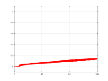 |
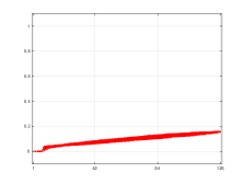
Finally, we consider the dataset FRED-MD described by McCracken and Ng (2016) consisting of times series covering both the real and nominal sectors of the U.S. economy and including also labor market indicators, and financial variables.111See https://research.stlouisfed.org/econ/mccracken/fred-databases/ The data is transformed to stationarity and missing values are imputed by means of the routines made available by McCracken and Ng (2016), which produces a balanced panel, with a sample running from April 1959 through March 2024, for an observation period of time points. The cross-sectional ordering, in this dataset, is fully arbitrary, hence meaningless. Standard methods (Bai and Ng, 2002) for determining the number of factors point to as much as factors. In Figure 3 we show the evolution for increasing of the eigenvalues , (all normalized by ) of when considering 100 random permutations of the cross-section. Once again, we see that the evolution of all eigenvalues is always well described by a linear divergence in , despite having different slopes due to the fact that eigenvalues are distinct.
Inspection of Figure 3 suggests that the last two or three factors are “weakly influential” (sufficiently so, however, for being detected by the Bai and Ng, 2002, method), and one may be tempted to consider them as rate-weak. Deciding about linear or sublinear divergence—in particular, testing the hypothesis of a rate-weak factor against rate-strong alternatives or estimating the value in a sublinear rate —is extremely delicate. In view of Sections 6.2 and 7 below, the issue, however, is probably of limited practical importance.
6.2 Factors and cross-sectional permutations: exchangeability
Distributional symmetries and group invariance properties are among the most convincing, irrefutable, and forceful arguments giving statistical inference problems a structure which, when it exists, dramatically impacts its solutions. Invariance arguments have a long history in mathematical statistics (see Chapter 6 in Lehmann and Romano (2024)); their pertinence, in a broad variety of problems, has been highlighted recently in Austern and Orbanz (2022).
Stationarity is one of those fundamental invariance properties and, under our fully nonparametric approach (no parameters), is the only assumption we are imposing in order to obtain a factor model decomposition. Namely, we assume that the observed panel is the finite realization of a stochastic process of the form in the class of real-valued second-order time-stationary processes indexed on . Second-order stationarity imposes a restriction (stationarity) on time dependence, namely,
Assumption 1.
The stochastic process is second-order stationary—namely, for any in , any , and any lag , .
This, however, does not say anything about cross-sectional dependence and, in particular, does not reflect the irrelevance of cross-sectional ordering. If that irrelevance is to be incorporated into the assumptions, the class has to be restricted further by imposing (second-order) cross-sectional exchangeability—another strong structural invariance property (of the same nature as (second-order) time-stationarity) discussed in Austern and Orbanz (2022); that assumption of exchangeability has been used in Barigozzi et al. (2024) to derive very complete asymptotic distributional results for the GDFM estimators of Forni et al. (2015, 2017).
Assumption 2.
The stochastic process is (second-order) cross-sectionally exchangeable—namely, for any , any -tuple , and any permutation in the set of the permutations of the integers , the distribution (the second-order moments) of the -dimensional stochastic processes
are the same.
Clearly, exchangeability implies second-order exchangeability, viz. for any and in , any and in , and any permutation . While second-order exchangeability, just as second-order stationarity, is mathematically sufficient for our needs, “full” exchangeability and “full” stationarity are the most natural and intuitively justifiable assumptions here. Denote by the class of second-order stationary second-order exchangeable processes .
Let us show that, under exchangeability, eigenvalue divergence only can be linear in .
The process can be rewritten as , emphasizing the fact that it can be considered as an infinite-dimensional time series. Its distribution then is naturally described as resulting from a two-step random mechanism: (Step I) the stochastic selection, via some unspecified distribution , of the distributional features , say, of the infinite-dimensional time series , followed by (Step II) a realization over time of the same.
A more formal description of Step I can be given as follows. Consider the space
equipped with the -field of all Borel (with respect to the topology of weak convergence) sets. Denoting by a distribution over some adequate probability space , let denote a measurable map from to : then is the random distribution of an infinite-dimensional time series, the spectral density matrices and covariance matrices of which are random as well, and so are random, as well as also their eigenvalues and .
The distribution here plays the role of a nuisance. Statistical practice in such cases consists in conducting inference on the realization observed in Step II conditional on the (unobserved) result of Step I (see, e.g., Chapter 10 of Lehmann and Romano (2024)), so that needs no further description. Under such conditional approach, the random distribution of the process of which the observed panel is a finite realization is treated as unknown but fixed. Hence , , and their eigenvalues are random variables treated as unknown but fixed quantities on which conditions as (3.4) or (4.3) are imposed: under unconditional form, these conditions actually should be imposed -almost surely.
Now, for simplicity, let us consider the first eigenvalue of the (conditional on the result of Step I) covariance matrix . Let , denote the contribution of cross-sectional item to . Then, . Denote by the expectation associated with : due to exchangeability, does not depend on . Hence, . Since is a nonnegative variable, two cases are possible. Either -a.s., and a.s. is -a.s. bounded as ; or and explodes at rate , which is incompatible with -a.s. with for and for . This precludes non-linear growth of . A similar reasoning holds for , , as well as for the dynamic eigenvalues .
If the irrelevance of the cross-sectional ordering is taken into account, thus, rate-weak factors are nowhere—much ado about nothing! Note, moreover, that if is bounded as , is a constant.
7 Undetected factors: “don’t throw out the baby with the bathwater!”
Onatski (2012)’s justification for considering rate-weak factors, however, is more subtle. His claim is that weak-factor asymptotics provide a better approximation in a finite- situation where the smallest linearly divergent eigenvalues do not separate well from the bulk of bounded eigenvalues. This is what is to be faced in the empirical exercise shown in Figure 3. He does not require, thus, the presence of a “genuinely rate-weak” factor, but uses rate-weak asymptotics as a tool for improved detection and estimation of these hardly detectable strong factors.
One may wonder, though, whether this is worth the effort. Identifying hardly detectable factors and incorporating them in the common space, indeed, has limited practical impact—provided, however, that factor models are not considered as a dimension-reduction technique throwing away the idiosyncratic—an attitude that is adopted by several authors.
Whether static or dynamic, undetected factors, indeed, are not lost, but wrongly left in the empirical idiosyncratic space. In a dimension-reduction perspective, the common component is considered an approximation of the high-dimensional observation which, being reduced rank, is more tractable than itself. The idiosyncratic then is discarded as if it were a negligible error term—a regrettable terminology used by some authors, mainly in the classical literature. This may be legitimate in specific datasets and is common practice, e.g., in macroeconometrics, where it seems that , indeed, safely can be neglected so that forecasting boils down to forecasting (Boivin and Ng, 2006; Luciani, 2014).
In many cases, however, needs not be small and may be strongly autocorrelated. Its empirical version, moreover, may contain undetected (rate-strong, but weakly influential) factors and discarding it is potentially quite damaging, e.g. in a prediction context. This is often the case in financial applications dealing with panels of volatility measures (Herskovic et al., 2016; Barigozzi and Hallin, 2017, 2020).
Rather than a dimension reduction technique, factor models, actually, should be considered a “divide and conquer” procedure where the common and the idiosyncratic are analyzed via distinct appropriate methods—reduced-rank-process techniques for the common, taking advantage of the strong cross-correlations, and componentwise or sparse techniques for the idiosyncratic, where no advantage can be gained from the negligible potential cross-correlations. The resulting analyses, at the end of the day, are to be brought back together: for instance, once forecasts and of the common and the idiosyncratic values at time have been obtained, their sum should be used as a predictor for . This point is clearly made by Fan et al. (2023) in the context of approximate static factor models and by Barigozzi et al. (2024) for the GDFM.
Now, undetected factors remain undetected because their empirical finite- cross-correlations are “small.” The benefits of detecting such factors and incorporating them into the common component is that their cross-correlations, there, would be exploited—which they are not in a componentwise or sparse analysis of the idiosyncratic. Since, however, these cross-correlations are too small to be detected, these benefits are small, too: leaving them in the idiosyncratic is basically harmless—as long as the idiosyncratic is not discarded!
The problem of undetected factors, thus, perhaps, is not as crucial, in practice, as it seems: if a factor gets undetected, the benefits of correctly identifying it as a factor are negligible.
8 Conclusions
This paper is dealing with several fundamental issues in the theory and practice of factor models. Its main conclusions are as follows.
-
(i)
Since, as shown by Gersing et al. (2023), it is nesting the classical and widespread static model of Chamberlain (1983) and Chamberlain and Rothschild (1983), the General Dynamic Factor Model of Forni et al. (2000) is uniformly preferable—the benefit being the incorporation into the common space of the GRD-weak factors which, in the static approach, are treated as idiosyncratic;
-
(ii)
under the (natural) assumption of cross-sectional exchangeability, rate-weak and rate-superstrong factors, whether static or dynamic, “are nowhere”;
-
(iii)
Gersing-Rust-Deistler-weak factors “are everywhere,” but are incorporated into the space of common components in the GDFM approach—which explains the empirical finding that the dynamic approach outperforms the static one even when the assumptions of the static factor model are satisfied;
-
(iv)
factor models are not a dimension-reduction technique and idiosyncratic components (which are not error terms) should not be discarded, as they may be large and have high predictive power;
-
(v)
in particular, estimated idiosyncratic components may contain undetected rate-strong factors: provided that idiosyncratic components are not discarded, these undetected factors are not lost, though.
These conclusions are likely to extend to matrix- and tensor-valued factor models, and to spatio-temporal ones, for which, however, a dynamic approach similar to the GDFM still needs to be developed.
References
- Amemiya et al. (1987) Amemiya, Y., W. A. Fuller, and S. G. Pantula (1987). The asymptotic distributions of some estimators for a factor analysis model. Journal of Multivariate Analysis 22, 51–64.
- Anderson and Rubin (1956) Anderson, T. W. and H. Rubin (1956). Statistical inference in factor analysis. In Proceedings of the third Berkeley symposium on mathematical statistics and probability, Volume 5, pp. 111–150.
- Ando and Bai (2017) Ando, T. and J. Bai (2017). Clustering huge number of financial time series: A panel data approach with high-dimensional predictors and factor structures. Journal of the American Statistical Association 112, 1182–1198.
- Austern and Orbanz (2022) Austern, M. and P. Orbanz (2022). Limit theorems for distributions invariant under groups of transformations. The Annals of Statistics 50, 1960–1991.
- Bai (2003) Bai, J. (2003). Inferential theory for factor models of large dimensions. Econometrica 71, 135–171.
- Bai and Li (2016) Bai, J. and K. Li (2016). Maximum likelihood estimation and inference for approximate factor models of high dimension. The Review of Economics and Statistics 98, 298–309.
- Bai and Ng (2002) Bai, J. and S. Ng (2002). Determining the number of factors in approximate factor models. Econometrica 70, 191–221.
- Bai and Ng (2006) Bai, J. and S. Ng (2006). Confidence intervals for diffusion index forecasts and inference for factor augmented regressions. Econometrica 74, 1133–1150.
- Bai and Ng (2023) Bai, J. and S. Ng (2023). Approximate factor models with weaker loadings. Journal of Econometrics 235, 1893–1916.
- Barigozzi et al. (2024) Barigozzi, M., H. Cho, and D. Owens (2024). FNETS: Factor-adjusted network estimation and forecasting for high-dimensional time series. Journal of Business & Economic Statistics 42, 890–902.
- Barigozzi and Farnè (2024) Barigozzi, M. and M. Farnè (2024). An algebraic estimator for large spectral density matrices. Journal of the American Statistical Association 119, 498–510.
- Barigozzi and Hallin (2017) Barigozzi, M. and M. Hallin (2017). Generalized dynamic factor models and volatilities: estimation and forecasting. Journal of Econometrics 201, 307–321.
- Barigozzi and Hallin (2020) Barigozzi, M. and M. Hallin (2020). Generalized dynamic factor models and volatilities: Consistency, rates, and prediction intervals. Journal of Econometrics 216, 4–34.
- Barigozzi et al. (2024) Barigozzi, M., M. Hallin, M. Luciani, and P. Zaffaroni (2024). Inferential theory for generalized dynamic factor models. Journal of Econometrics 239, 105422.
- Barigozzi et al. (2023) Barigozzi, M., D. La Vecchia, and H. Liu (2023). General spatio-temporal factor models for high-dimensional random fields on a lattice. Technical Report arXiv:2312.02591.
- Barigozzi and Luciani (2024) Barigozzi, M. and M. Luciani (2024). Quasi maximum likelihood estimation and inference of large approximate dynamic factor models via the EM algorithm. Technical Report arXiv:1910.03821.v4.
- Bartlett (1937) Bartlett, M. (1937). The statistical conception of mental factors. British Journal of Psychology 28, 97–104.
- Bartlett (1938) Bartlett, M. (1938). Methods of estimating mental factors. Nature 141, 609–610.
- Boivin and Ng (2006) Boivin, J. and S. Ng (2006). Are more data always better for factor analysis? Journal of Econometrics 132, 169–194.
- Brezis (2011) Brezis, H. (2011). Functional Analysis, Sobolev Spaces, and Partial Differential Equations. Springer.
- Brillinger (1981) Brillinger, D. R. (1981). Time Series: Data Analysis and Theory. Classics in Applied Mathematics. SIAM.
- Chamberlain (1983) Chamberlain, G. (1983). Funds, factors and diversification in arbitrage pricing models. Econometrica 51, 1305–1323.
- Chamberlain and Rothschild (1983) Chamberlain, G. and M. Rothschild (1983). Arbitrage, factor structure, and mean-variance analysis on large asset markets. Econometrica 51, 1281–1323.
- De Mol et al. (2008) De Mol, C., D. Giannone, and L. Reichlin (2008). Forecasting using a large number of predictors: Is Bayesian shrinkage a valid alternative to principal components? Journal of Econometrics 146, 318–328.
- Doz et al. (2011) Doz, C., D. Giannone, and L. Reichlin (2011). A two-step estimator for large approximate dynamic factor models based on kalman filtering. Journal of Econometrics 164, 188–205.
- Doz et al. (2012) Doz, C., D. Giannone, and L. Reichlin (2012). A quasi maximum likelihood approach for large approximate dynamic factor models. The Review of Economics and Statistics 94(4), 1014–1024.
- Engle and Watson (1981) Engle, R. and M. Watson (1981). A one-factor multivariate time series model of metropolitan wage rates. Journal of the American Statistical Association 76, 774–781.
- Evans (2010) Evans, L. (2010). Partial Differential Equations. American Mathematical Society.
- Fan et al. (2023) Fan, J., R. P. Masini, and M. C. Medeiros (2023). Bridging factor and sparse models. The Annals of Statistics 51, 1692–1717.
- Fan et al. (2024) Fan, J., Y. Yan, and Y. Zheng (2024). When can weak latent factors be statistically inferred? Technical Report arXiv:2407.03616v1.
- Forni et al. (2009) Forni, M., D. Giannone, M. Lippi, and L. Reichlin (2009). Opening the black box: Structural factor models with large cross sections. Econometric Theory 25, 1319–1347.
- Forni et al. (2018) Forni, M., A. Giovannelli, M. Lippi, and S. Soccorsi (2018). Dynamic factor model with infinite-dimensional factor space: forecasting. Journal of Applied Econometrics 33, 625–642.
- Forni et al. (2000) Forni, M., M. Hallin, M. Lippi, and L. Reichlin (2000). The generalized dynamic-factor model: Identification and estimation. Review of Economics and Statistics 82, 540–554.
- Forni et al. (2004) Forni, M., M. Hallin, M. Lippi, and L. Reichlin (2004). The generalized dynamic factor model: consistency and rates. Journal of Econometrics 119, 231–255.
- Forni et al. (2015) Forni, M., M. Hallin, M. Lippi, and P. Zaffaroni (2015). Dynamic factor models with infinite-dimensional factor spaces: One-sided representations. Journal of Econometrics 185, 359–371.
- Forni et al. (2017) Forni, M., M. Hallin, M. Lippi, and P. Zaffaroni (2017). Dynamic factor models with infinite-dimensional factor space: asymptotic analysis. Journal of Econometrics 199, 74–92.
- Forni and Lippi (2001) Forni, M. and M. Lippi (2001). The generalized dynamic factor model: representation theory. Econometric Theory 17, 1113–1141.
- Freyaldenhoven (2022) Freyaldenhoven, S. (2022). Factor models with local factors: Determining the number of relevant factors. Journal of Econometrics 229, 80–102.
- Gersing et al. (2023) Gersing, P., C. Rust, and M. Deistler (2023). Weak factors are everywhere. arXiv preprint arXiv:2307.10067.
- Geweke (1977) Geweke, J. (1977). The dynamic factor analysis of economic time series. In In D.J. Aigner and A.S. Goldberger, Eds., Latent variables in socio-economic models, pp. 365–383. North Holland., Amsterdam.
- Hallin et al. (2018) Hallin, M., S. Hörmann, and M. Lippi (2018). Optimal dimension reduction for high-dimensional and functional time series. Statistical Inference for Stochastic Processes 21, 385–398.
- Hallin and Lippi (2013) Hallin, M. and M. Lippi (2013). Factor models in high-dimensional time series—a time-domain approach. Stochastic Processes and Their Applications 123, 2678–2695.
- Hallin and Liška (2007) Hallin, M. and R. Liška (2007). The generalized dynamic factor model: determining the number of factors. Journal of the American Statistical Association 102, 603–617.
- Hallin and Liška (2011) Hallin, M. and R. Liška (2011). Dynamic factors in the presence of blocks. Journal of Econometrics 163, 29–41.
- Herskovic et al. (2016) Herskovic, B., B. Kelly, H. Lustig, and S. Van Nieuwerburgh (2016). The common factor in idiosyncratic volatility: Quantitative asset pricing implications. Journal of Financial Economics 119, 249–283.
- Hotelling (1933a) Hotelling, H. (1933a). Analysis of a complex of statistical variables into principal components, Part 1. Journal of Educational Psychology 24, 417–441.
- Hotelling (1933b) Hotelling, H. (1933b). Analysis of a complex of statistical variables into principal components, Part 2. Journal of Educational Psychology 25, 498–520.
- Jöreskog (1969) Jöreskog, K. (1969). A general approach to confirmatory maximum likelihood factor analysis. Psychometrika 34, 183–202.
- Jöreskog (2007) Jöreskog, K. (2007). Factor analysis and its extensions. In In R. Cudeck and R.C. MacCallum, Eds, Factor Analysis at 100: Historical Developments and Future Directions, pp. 47–77. Lawrence Erlbaum Associates, Mahwah, N.J.
- Lam and Yao (2012) Lam, C. and Q. Yao (2012). Factor modeling for high-dimensional time series: inference for the number of factors. The Annals of Statistics 40, 694–726.
- Lawley and Maxwell (1971) Lawley, D. and A. Maxwell (1971). Factor Analysis as a Statistical Method, 2nd Edition. London: Butterworths.
- Lehmann and Romano (2024) Lehmann, E. and J. Romano (2024). Testing Statistical Hypotheses, 3rd Edition. Springer.
- Luciani (2014) Luciani, M. (2014). Forecasting with approximate dynamic factor models: the role of non-pervasive shocks. International Journal of Forecasting 30, 20–29.
- McCracken and Ng (2016) McCracken, M. W. and S. Ng (2016). FRED-MD: A monthly database for macroeconomic research. Journal of Business & Economic Statistics 34, 574–589.
- Moench et al. (2013) Moench, E., S. Ng, and S. Potter (2013). Dynamic hierarchical factor models. Review of Economics and Statistics 95, 1811–1817.
- Onatski (2012) Onatski, A. (2012). Asymptotics of the principal components estimator of large factor models with weakly influential factors. Journal of Econometrics 168, 244–258.
- Quah and Sargent (1993) Quah, D. and T. Sargent (1993). A dynamic index model for large cross sections. In In J.H. Stock and M.W. Watson, Eds., Business Cycles, Indicators and Forecasting, pp. 285–306. University of Chicago Press.
- Sargent and Sims (1977) Sargent, T. and C. Sims (1977). Business cycle modeling without pretending to have too much a priori economic theory. In In C.A. Sims, Ed., New Methods in Business Cycle Research, pp. 45–109. Federal Reserve Bank of Minneapolis.
- Shumway and Stoffer (1982) Shumway, R. and D. Stoffer (1982). An approach to time series smoothing and forecasting using the EM algorithm. Journal of Time Series Analysis 3, 253–264.
- Spearman (1904) Spearman, C. (1904). General intelligence, objectively determined and measured. The American Journal of Psychology 15, 201–292.
- Stock and Watson (2002a) Stock, J. H. and M. W. Watson (2002a). Forecasting using principal components from a large number of predictors. Journal of the American Statistical Association 97, 1167–1179.
- Stock and Watson (2002b) Stock, J. H. and M. W. Watson (2002b). Macroeconomic forecasting using diffusion indexes. Journal of Business & Economic Statistics 20, 147–162.
- Uematsu and Yamagata (2022) Uematsu, Y. and T. Yamagata (2022). Estimation of sparsity-induced weak factor models. Journal of Business & Economic Statistics 41, 213–227.
- Watson and Engle (1983) Watson, M. and R. Engle (1983). Alternative algorithms for the estimation of dynamic factor, mimic and varying coefficient regression models. Journal of Econometrics 23, 385–400.
Appendix. The static approximate factor model revisited.
In this appendix, we formally establish the fact that the representation result (4.2), along with assumption (4.3) on the eigenvalues , , of the covariance matrix of imply that the assumptions (a)–(g) of the static approximate factor model (2.1) of Chamberlain and Rothschild are satisfied. Essentially, this consists in showing that the covariance matrices and of the statically common and idiosyncratic components and defined in (4.2) and their eigenvalues are such that
-
(i)
is of the form for some vector and some random vector satisfying assumption (c) in Section 2.1;
-
(ii)
the eigenvalues of tend to infinity as (it readily follows from (i) that for all );
-
(iii)
the first (largest) eigenvalue of is bounded as .
Below, to keep the notation simple, we denote by , , and the Hilbert spaces , , and of Section 4. The unit vector corresponding to (the standardized version of with variance ) is denoted by . Denoting by the principal components of , write for the (closed) -dimensional subspace of spanned by and for the (closed) subspace of spanned by
Recall that an infinite-dimensional Hilbert space admits two distinct topologies, the weak topology and the strong one. In the strong topology, convergence is associated with the norm: converges strongly to (notation: ) if as —strong convergence, in our case, thus, is convergence in quadratic mean (q.m. convergence). Weak convergence of to (notation: ) is characterized by the fact that (in our case, Cov Cov) for any as for any as . For finite-dimensional Hilbert spaces, the weak and strong topologies coincide. An important (Bolzano-Weierstrass-type) property is that any bounded sequence (bounded in the norm—in our case, Var() bounded) admits a subsequence222Any subsequence of a sequence of elements of , of course, still is a sequence of elements of . converging weakly to some —see, e.g., section D.4 on page 639 of Evans (2010) or Theorem 3.18 in Brezis (2011). Finally, recall that orthogonal projections, in , are linear continuous operators.
The proof is organised in four steps.
(1) We first characterize in terms of the limits of sequences of standardized elements of . By definition, the elements (with variance ) of are such that is the strong limit (the q.m. limit), as , of sequences where with has variance as . Note that , in this definition, can be replaced with provided that remains bounded away from zero and infinity. Denote by the collection of such sequences: , thus, iff is the strong limit of a sequence . Clearly, for , the sequences of standardized principal components of , hence the sequences of standardized elements of , belong to . Denoting by the collection of such sequences, let us show that iff is the strong limit of a sequence , that is,
(note that can be replaced with where is a subsequence of ).
To show this, consider such that . Each canonically decomposes into a sum with and orthogonal to and ; the variances tend to infinity while the variances remain bounded as . Hence, if is the strong limit of a sequence of , it is also the strong limit of the sequence of .
(2) Next, we show that a subsequence of the -tuple converges weakly to an orthogonal system . Since for each the -tuple is an orthonormal basis of , any in is such that is a linear combination of . As an -tuple of bounded sequence, contains a subsequence converging weakly to some -tuple . Weak convergence implies the convergence of covariances, and hence preserves orthogonality: indeed,
The -tuple , thus, is an orthogonal basis of the -dimensional space it is spanning.
(3) Let us conclude that coincides with , hence has finite dimension . Denote by Proj the orthogonal projection operator from to . As a projection, the mapping Proj is linear and continuous. Hence,
where the latter convergence takes place in a finite-dimensional space, so that it also holds in the strong topology: . Hence, the strong limits of sequences also are strong limits of the sequence of their projections on , and so are the limits of strongly convergent sequences thereof. Since strong convergence implies convergence of the norms and Var()=1 for all , Var() =1 as well. Conversely, any element in being a linear combination of (or the limit of a strongly convergent sequence thereof), it is the strong limit of the sequence of the projections on of the same linear combinations of (or the limit of strongly convergent sequence thereof). As a consequence, iff , hence itself, is an element of : we thus have .
(4) The static factor model decomposition of follows as a corollary. Denote by (and call static factors) an arbitrary orthonormal basis of the -dimensional space . Since and , for with , . This takes care of (i).
(5) To conclude, let us show that (ii) has exactly divergent eigenvalues while (iii) the eigenvalues of all are bounded. Let us assume that the number of diverging eigenvalues of is strictly less than . Since decomposes into and has diverging eigenvalues, the Weyl inequalities imply that the first eigenvalue of tends to infinity as . Then, there exists a sequence with and such that the variance of tends to infinity as . Since is the projection of on , also is a linear combination of and (the eigenvalues of a nondegenerate projection operator are either 1 or zero, and cannot all be zero) . Hence, the sequence , where each has variance one, is in . This bounded sequence contains a subsequence converging weakly to some ; since each is in , hence orthogonal to , so is the weak limit . Proceeding as in (3), it can be shown that this also is the strong limit of a sequence of elements of , hence belongs to ; moreover, since the convergence is strong, Var()=1. The intersection of and being , this implies . This, however, is incompatible with Var()=1. Therefore, the number of diverging eigenvalues of cannot be strictly less than . The Weyl inequalities and the fact that then imply that all eigenvalues of are bounded as . Claims (ii) and (iii) follow.