Unified Implementation of Relativistic Wave Function Methods: 4C-iCIPT2 as a Showcase

Ning Zhang111Current address: Division of Chemistry and Chemical Engineering, California Institute of Technology, Pasadena, CA 91125, USA    Wenjian Liu liuwj@sdu.edu.cn Qingdao Institute for Theoretical and Computational Sciences, School of Chemistry and Chemical Engineering, Shandong University, Qingdao, Shandong 266237, China
Abstract

In parallel to the unified construction of relativistic Hamiltonians based solely on physical arguments [J. Chem. Phys. 160, 084111 (2024)], a unified implementation of relativistic wave function methods is achieved here via programming techniques (e.g., template metaprogramming and polymorphism in C++). That is, once the code for constructing the Hamiltonian matrix is made ready, all the rest can be generated automatically from existing templates used for the nonrelativistic counterparts. This is facilitated by breaking a second-quantized relativistic Hamiltonian down to diagrams that are topologically the same as those required for computing the basic coupling coefficients between spin-free configuration state functions (CSF). Moreover, both time reversal and binary double point group symmetries can readily be incorporated into molecular integrals and Hamiltonian matrix elements. The latter can first be evaluated in the space of (randomly selected) spin-dependent determinants and then transformed to that of spin-dependent CSFs, thanks to simple relations in between. As a showcase, we consider here the no-pair four-component relativistic iterative configuration interaction with selection and perturbation correction (4C-iCIPT2), which is a natural extension of the spin-free iCIPT2 [J. Chem. Theory Comput. 17, 949 (2021)], and can provide near-exact numerical results within the manifold of positive energy states (PES), as demonstrated by numerical examples.

1 INTRODUCTION

Accurate descriptions of the electronic structure of systems containing heavy elements should in principle treat relativistic, correlation, and even quantum electrodynamics (QED) effects simultaneously1, so as to match experimental measurements without relying on error compensations2, 3, 4. Both relativistic and leading QED effects can be built into the Hamiltonian5, 6, 7, 8, 9, 10, 11, whereas correlation is carried on by the wave function parameterized by a particular ansatz. Given the complete ‘Hamiltonian ladder’7, 6, from which one can pick up the right Hamiltonian according to the target problem and accuracy, the task remains to search for suitable parameterizations of the wave function, so as to describe electron correlation as accurately as possible. Since many-electron relativistic Hamiltonians can only be formulated properly in Fock space 5, 6, 7, 8, 9, 10, 11, 12, 13, explicitly correlated wave function methods are excluded from the outset, unless special care is taken13, 14, 15, 16, 17. In contrast, any orbital product-based wave function ansatz can be combined with any second-quantized relativistic Hamiltonian. The available relativistic wave function methods can be classified into two categories, with spinors or scalar orbitals as building units. The former can further be classified into two categories, four-component (4C) or two-component (2C). Since the two sets are indistinguishable in the correlation step after integral transformations, they can be regarded as equivalent from the computational point of view. Essentially all variants of wave function methods developed in the nonrelativistic regime have been transferred to the 4C/2C domain under the no-pair approximation (NPA), including multiconfiguration self-consistent field (SCF) 18, 19, 20, 21, 22, 23, 24, 25, many-body perturbation theory26, 27, 28, 29, 30, 31, 32, coupled-cluster33, 34, 35, 36, 37, 38, 39, 40, 41, 42, 43, 44, 45, 46, 47, 48, 49, 50, 51, configuration interaction (CI)52, 53, 54, 55, 56, 57, 58, 59, 60, 61, 62, density-matrix renormalization group63, 64, 65, and full configuration interaction (FCI) quantum Monte Carlo66. It deserves to be mentioned that the correlation contribution of negative energy states (NES) can readily be accounted for in both the 4C and 2C frameworks, so as to go beyond the NPA5, 6, 67.

Although methods that start with scalar orbitals and treat SOC in the correlation step are sometimes also termed two-component, we prefer to call them one-component (1C) to distinguish them from those working with two-component spinors. The former involve spin-separated Hamiltonians, whereas the latter do not. Such methods can also be classified into two categories, one- or two-step68. The former type of approaches69, 70, 71, 72, 73, 74, 75, 76, 77, 78, 79, 80, 81, 82, 83 aims to treat spin-orbit and electron-electron interactions on an equal footing, whereas the latter type of approaches 84, 85, 86, 87, 88, 89, 90, 91, 92, 93, 94, 95, 96, 97, 98, 99, 100, 101, 102, 103, 104, 105 amounts to treating SOC after correlation, by constructing and diagonalizing an effective spin-orbit Hamiltonian matrix over a set of close-lying correlated scalar states. It is obvious that such two-step-1C approaches work well only when SOC and correlation are roughly additive. Of course, they become identical with the one-step-1C approaches if all correlated scalar states from the space spanned by individual configurations are included. It is also true that the one-step-1C approaches can approach the 4C/2C ones in the no-pair FCI limit, particularly when spin orbital relaxations induced by SOC are further accounted for by variational optimizations106, 107. However, in practice, great care has to be taken of the choice of active (scalar) orbitals83 and even of basis sets107 to avoid spurious results, especially for spin-orbit splittings of $np$ ($n\geq 5$) orbitals.

Notwithstanding the above developments, relativistic wave function methods that are highly accurate for strongly correlated, especially open-shell, systems containing heavy elements are still highly desired. Considering that relativity (especially SOC) and correlation reside in different regions of the Hilbert space due to their very different physical origins (primarily one-body magnetic vs. primarily two-body Coulomb interactions), such methods must be self-adaptive and balanced, based on some selection procedure. As an attempt to this end, we consider here the 4C variant of iCIPT2 (iterative configuration interaction (iCI)108 with selection and second-order perturbation correction)109, 110, which has proved to be one of the most accurate and efficient methods111, and is applicable to arbitrary open-shell systems thanks to use of configuration state functions (CSF) as the many-electron basis functions (MBF). Both time reversal and double group symmetries ought to be incorporated into 4C-iCIPT2, so as to facilitate not only the computation but also the state assignment (see Appendices A and B). It turns out that the implementation of 4C-iCIPT2 can be simplified greatly by leveraging the power of meta-programming furnished by C++: once the code for constructing the relativistic Hamiltonian matrix is made ready, all the rest can be generated automatically from the existing templates used for iCITP2, without the need to distinguish between complex and real algebras. In particular, sophisticated techniques available in iCIPT2, e.g., memory allocation, loop unrolling, data sorting, and intermediates recycling, etc., can directly be transferred to 4C-iCIPT2. Therefore, a unified implementation of relativistic and nonrelativistic wave function methods has been achieved, in parallel to the unified construction of relativistic Hamiltonians112. This is made possible only by invoking a diagrammatical representation of the relativistic Hamiltonian that is topologically the same as that employed in the unitary group approach113 for determining the basic coupling coefficients (BCC) between spin-free CSFs (cf. Sec. 2.3).

The rest of the paper is organized as follows. Sec. 2 is devoted to the theoretical aspects, including a brief discussion of relativistic Hamiltonians in Sec. 2.1, general structure of the Hamiltonian matrix in Sec. 2.2, and special treatment of Hamiltonian matrix elements in Sec. 2.4. The spin-free iCIPT2109, 110 is then recapitulated in Sec. 3, where the implementation of 4C-iCIPT2 is also presented. Some benchmark calculations are provided in Sec. 4. The paper is finally closed with concluding remarks in Sec. 5.

The Einstein summation convention over repeated indices is always employed.

2 THEORY

2.1 Relativistic Hamiltonians

As emphasized repeatedly12, 13, 5, 6, 9, 10, many-body relativistic Hamiltonians can only be formulated properly in Fock space, for all configuration space-based, first-quantized relativistic Hamiltonians suffer13, 5 from unphysical contaminations of negative energy states (NES) of the Dirac equation. As a matter of fact, by interpreting the solutions $\{\psi_{p}\}$ of the effective one-body Dirac equation

$\displaystyle h\psi_{p}$ $\displaystyle=\epsilon_{p}\psi_{p},\quad p\in\mbox{ PES, NES},$ (1)
$\displaystyle h$ $\displaystyle=D+U(\mathbf{r}),$ (2)
$\displaystyle D$ $\displaystyle=c\bm{\alpha}\cdot\bm{p}+\beta c^{2}+V_{\mathrm{nuc}},$ (3)
$\displaystyle\bm{\alpha}$ $\displaystyle=\begin{pmatrix}0&\bm{\sigma}\\ \bm{\sigma}&0\end{pmatrix},\quad\beta=\begin{pmatrix}1&0\\ 0&-1\end{pmatrix},\quad\bm{p}=-\mathbbm{i}\hbar\bm{\partial}$ (4)

as classical fields and second-quantizing them properly10, one can readily obtain the normal-ordered many-body relativistic quantum electrodynamics (QED) Hamiltonian

$\displaystyle H_{n}$ $\displaystyle=(h_{pq}+Q_{pq})\{E_{pq}\}_{n}+\frac{1}{2}g_{pq,rs}\{e_{pq,rs}\}_{n},\quad p,r,r,s\in\mbox{ PES, NES},$ (5)
$\displaystyle h_{pq}$ $\displaystyle=\langle\psi_{p}|h|\psi_{q}\rangle,\quad Q_{pq}=-\frac{1}{2}\bar{g}_{pq,ss}{\rm{sgn}}(\epsilon_{s}),$ (6)
$\displaystyle g_{pq,rs}$ $\displaystyle=(pq|V(1,2)|rs),\quad\bar{g}_{pq,rs}=g_{pq,rs}-g_{ps,rq},$ (7)
$\displaystyle E_{pq}$ $\displaystyle=a_{p}^{\dagger}a_{q},\quad e_{pq,rs}=a^{pr}_{qs}=E_{pq}E_{rs}-\delta_{qr}E_{ps}=e_{rs,pq}=-e_{ps,rq}=-e_{rq,ps},$ (8)

provided that the charge-conjugated contraction5

$\displaystyle\acontraction[0.5ex]{}{a^{p}}{}{a_{q}}a^{p}a_{q}$ $\displaystyle=-\acontraction[0.5ex]{}{a_{q}}{}{a^{p}}a_{q}a^{p}=\langle 0;\tilde{N}|\frac{1}{2}[a^{p},a_{q}]|0;\tilde{N}\rangle=-\frac{1}{2}\delta^{p}_{q}{\rm{sgn}}(\epsilon_{q}),\quad p,q\in\mbox{PES, NES},$ (9)

is employed when normal ordering with respect to $|0;\tilde{N}\rangle$, a reference that is built up with the NES of Eq. (1) and represents the filled Dirac sea when the number ($\tilde{N}$) of negative energy electrons approaches infinity. The so-obtained effective potential $Q$ (6) describes vacuum polarization and electron self-energy, the genuine QED effect5. It has recently been shown decisively114, 115 that the Hamiltonian (5) is the only correct and complete QED Hamiltonian (in the form of eigenvalue problem), at variance with other proposals116, 117.

Although relativistic, correlation, and QED effects can in principle be treated on an equal footing1, for the time being we ignore QED effects and instead consider the no-pair approximation. That is, the QED Hamiltonian (5) is to be simplified to

$\displaystyle H_{+}$ $\displaystyle=h_{pq}E_{pq}+\frac{1}{2}g_{pq,rs}e_{pq,rs},\quad p,q,r,s\in\mbox{ PES},$ (10)

which accounts only for electron correlation within the manifold of positive energy states (PES), mediated by the instantaneous electron-electron interaction

$\displaystyle V(1,2)$ $\displaystyle=\frac{1}{r_{12}}+\mathrm{c_{g}}\frac{\bm{\alpha}_{1}\cdot\bm{\alpha}_{2}}{r_{12}}+\mathrm{c_{b}}\bm{\alpha}_{1}\cdot\frac{\bm{r}_{12}\otimes\bm{r}_{12}}{r_{12}^{3}}\cdot\bm{\alpha}_{2},$ (11)

which reduces to the Coulomb (C), Coulomb-Gaunt (CG), and Coulomb-Breit (CB) interactions by setting $(\mathrm{c_{g}},\mathrm{c_{b}})$ to $(0,0)$, $(-1,0)$, and $(-1/2,-1/2)$, respectively. To avoid over notation, we will denote the Coulomb and Gaunt/Breit electron repulsion integrals (ERI) simply as $(pq|rs)$ and $(p\bm{\alpha}q|r\bm{\alpha}s)$, respectively. If wanted, the no-pair four-component Hamiltonian (10) can further be transformed to the quasi-four-component (Q4C)118, 119 and exact two-component (X2C)120, 121, 122 variants that can be constructed in a unified manner, based solely on physical arguments112.

In the absence of magnetic interactions, the Hamiltonians (2) and (10) commute with the time reversal operator $\mathcal{K}$ ($=-\mathbbm{i}\mathbf{I}_{2}\otimes\sigma_{y}K_{0}$). The spinors can therefore be grouped into Kramers pairs $\{\psi_{p},\psi_{\bar{p}}=\mathcal{K}\psi_{p}\}_{p=1}^{K_{P}}$. As shown in Appendix A.1, compared to the brute-force storage, the storage requirement for the ERIs can be reduced by a factor of 16 by making proper use of time reversal and permutation symmetries. Point group symmetries inherent in the ERIs are further revealed in Sec. A.2.

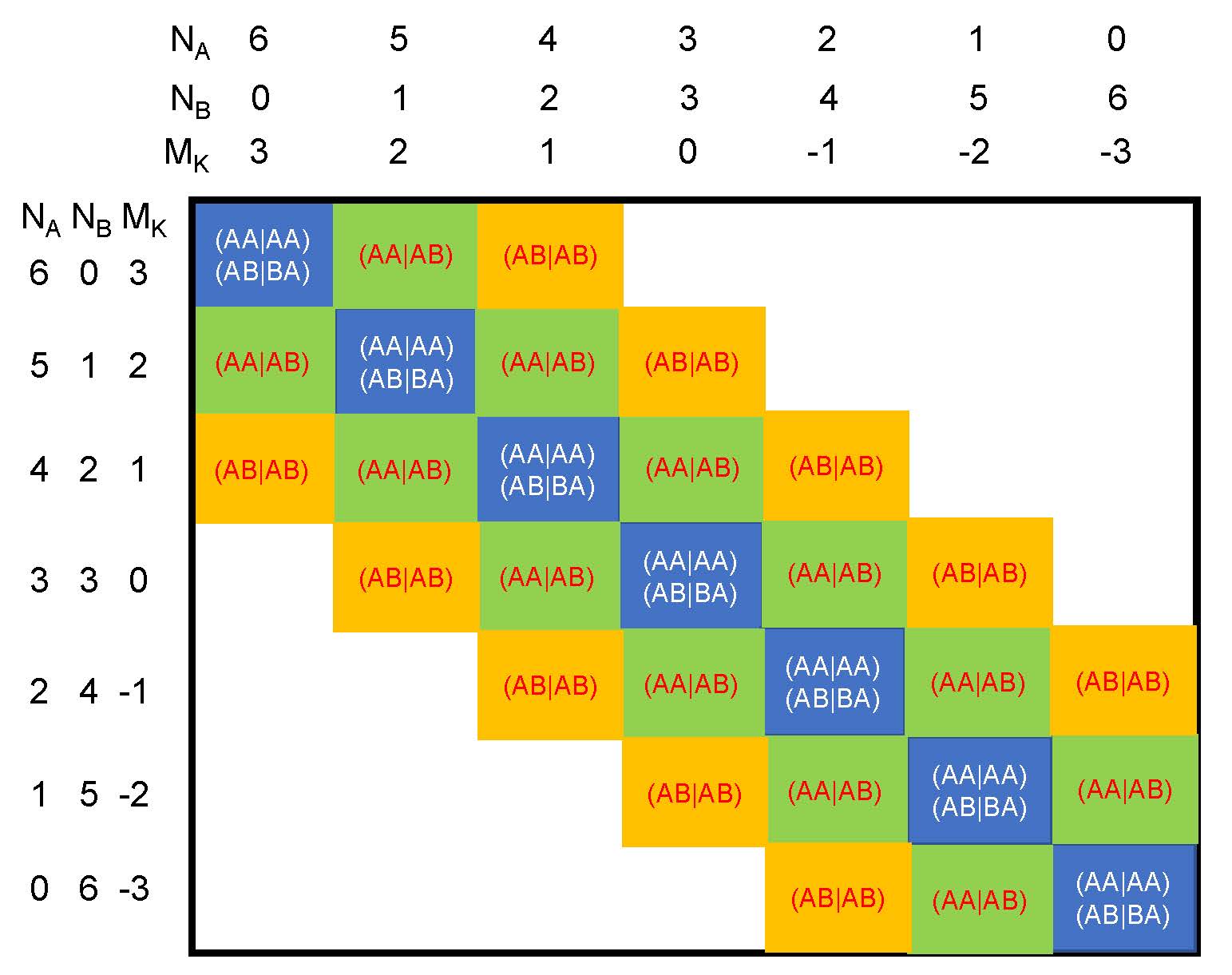
2.2 General Structure of Hamiltonian Matrix

Consider all possible Slater determinants (SD) that can be constructed by distributing $N$ electrons in a given set of $K_{P}$ Kramers pairs $\{\psi_{p},\psi_{\bar{p}}=\mathcal{K}\psi_{p}\}_{p=1}^{K_{P}}$. Every SD can be characterized by the pseudo-quantum number $M_{K}=(N_{A}-N_{B})/2$, with $N_{A}$ and $N_{B}$ ($=N-N_{A}$) being the numbers of unbarred (A) and barred (B) spinors. If SDs of the same $M_{K}$ are grouped into one set (of size $C_{K_{P}}^{N_{A}}C_{K_{P}}^{N_{B}}$) and different sets are ordered in a descendent order of $M_{K}$, the Hamiltonian matrix will become block pentadiagonal123 (see Fig. 1), for the matrix elements are zero when two sets of SDs differ in their $M_{K}$ values by more than two and are hence connected by more than double excitations. For the main diagonal blocks with $|M_{K}(L)-M_{K}(M)|=0$, the matrix elements $H_{LM}$ consist of one-electron integrals of the type $\langle A|h|A\rangle$ and ERIs of the types $(AA|AA)$ and $(AB|BA)$ (see Sec. A.1). For the first off-diagonal blocks with $|M_{K}(L)-M_{K}(M)|=1$, the matrix elements $H_{LM}$ consist of one-electron integrals of the type $\langle A|h|B\rangle$ and ERIs of the type $(AA|AB)$, whereas for the second off-diagonal blocks with $|M_{K}(L)-M_{K}(M)|=2$, the matrix elements $H_{LM}$ consist of ERIs of the type $(AB|AB)$. Moreover, the following relations

$\displaystyle|\bar{M}\rangle$ $\displaystyle=\hat{\mathcal{K}}|M\rangle,\quad\hat{\mathcal{K}}|\bar{M}\rangle=(-1)^{N}|M\rangle,$ (12)
$\displaystyle|\bar{M}\rangle$ $\displaystyle=|M\rangle\mbox{ (closed-shell)},$ (13)
$\displaystyle\langle\bar{L}|H_{+}|\bar{M}\rangle$ $\displaystyle=\langle L|H_{+}|M\rangle^{*}=\langle M|H_{+}|L\rangle,$ (14)
$\displaystyle\langle\bar{L}|H_{+}|M\rangle$ $\displaystyle=(-1)^{N}\langle L|H_{+}|\bar{M}\rangle^{*}=(-1)^{N}\langle\bar{M}|H_{+}|L\rangle$ (15)

dictate that the Hamiltonian matrix has the following structure

$$\begin{pmatrix}\langle L|H_{+}|M\rangle&\langle L|H_{+}|\bar{M}\rangle\\ \langle\bar{L}|H_{+}|M\rangle&\langle\bar{L}|H_{+}|\bar{M}\rangle\end{pmatrix}=\begin{bmatrix}A_{LM}&B_{LM}\\ (-1)^{N}B_{LM}^{*}&A_{LM}^{*}\\ \end{bmatrix},\quad\mathbf{A}=\mathbf{A}^{\dagger},\quad\mathbf{B}=\mathbf{B}^{T},$$ (16)

which shows that the number of unique matrix elements can be reduced by a factor of two. For the case of even $N$, it is even possible to construct orthonormal, time-even (real-valued) scalar MBFs123

$$\left|M^{s}\right\rangle=\frac{i^{(1-s)/2}}{\sqrt{2\left(1+\delta_{M,\bar{M}}\right)}}(|M\rangle+s|\bar{M}\rangle),\quad s=\pm 1,$$ (17)

over which the Hamiltonian matrix become real and symmetric, viz.,

$\displaystyle\begin{pmatrix}\langle L^{+}|H_{+}|M^{+}\rangle&\langle L^{+}|H_{+}|M^{-}\rangle\\ \langle L^{-}|H_{+}|M^{+}\rangle&\langle L^{-}|H_{+}|M^{+}\rangle\end{pmatrix}=\begin{bmatrix}H^{++}_{LM}&H^{+-}_{LM}\\ H^{-+}_{LM}&H^{--}_{LM}\\ \end{bmatrix},$ (18)

where

$\displaystyle H^{++}_{LM}$ $\displaystyle=\operatorname{Re}\left(H_{LM}+H_{L\bar{M}}\right)/G_{LM}=H^{++}_{ML},$ (19)
$\displaystyle H^{+-}_{LM}$ $\displaystyle=-\operatorname{Im}\left(H_{LM}-H_{L\bar{M}}\right)/G_{LM}=H^{-+}_{ML},$ (20)
$\displaystyle H^{-+}_{LM}$ $\displaystyle=\operatorname{Im}\left(H_{LM}+H_{L\bar{M}}\right)/G_{LM}=H^{+-}_{ML},$ (21)
$\displaystyle H^{--}_{LM}$ $\displaystyle=\operatorname{Re}\left(H_{LM}-H_{L\bar{M}}\right)/G_{LM}=H^{--}_{ML},$ (22)
$\displaystyle G_{LM}$ $\displaystyle=\sqrt{\left(1+\delta_{L,\bar{L}}\right)\left(1+\delta_{M,\bar{M}}\right)}.$ (23)

As shown in Appendix B, a second pseudo-quantum number, $\tilde{M}_{K}=2M_{K}\mod 4$, can be invoked to classify the MBFs according to binary double point group symmetries. As a result, for both odd and even $N$, the combined use of time reversal and point group symmetries reduces the computational cost by the order of the given group (i.e., 2, 4, 4, 4, 8, 8, 8, and 16 for the $C_{1}^{\ast}$, $C_{i}$, $C_{2}^{\ast}$, $C_{s}^{\ast}$, $C_{2h}^{\ast}$, $C_{2v}^{\ast}$, $D_{2}^{\ast}$, and $D_{2h}^{\ast}$ point groups, respectively).

Refer to caption
Figure 1: Block pentadiagonal structure of relativistic Hamiltonian matrix over $M_{K}$-ordered determinants. The $(AA|AB)$ type of ERIs exist only for the $C_{1}^{\ast}$ and $C_{i}^{\ast}$ groups, and all the ERIs become real-valued for the $C_{2v}^{\ast}$, $D_{2}^{\ast}$, and $D_{2h}^{\ast}$ groups (cf. Appendix A.1).

2.3 Breakdown of Relativistic Hamiltonian

It has been shown109 that the spin-free, second-quantized Hamiltonian can be broken down to terms that have one-to-one correspondence with the diagrams employed in the unitary group approach113 for determining the basic coupling coefficients (BCC) between CSFs. In the first place, the breakdown classifies the Hamiltonian matrix elements $\langle I\mu|\hat{\mathcal{H}}|J\nu\rangle$ into distinct groups based on the excitation level (0, 1, or 2) from the ket orbital configuration (oCFG) $|J\rangle$ to the bra $|I\rangle$. Secondly, the common zero or doubly occupied orbitals in the bra and ket oCFGs can be deleted, ending up with reduced occupation tables (ROT) characterizing oCFG pairs. All oCFG pairs sharing the same ROT have the same BCCs, thereby avoiding repeated evaluations of the BCCs. Thirdly, a closed-shell reference oCFG can be introduced to simplify the evaluation of the Hamiltonian matrix elements over zero or singly excited oCFGs. It is shown here that such techniques can also be extended to the relativistic domain working with SDs though, by defining the occupation number (PON) of a Kramers pair $\mathcal{P}_{p}=(p,\bar{p})$ as $\tilde{n}_{p}=n_{p}+n_{\bar{p}}$. Different SDs $|J\nu\rangle$ generated from the same oCFG $|J\rangle$ share the same PONs but differ in their spinor occupations (SON).

The general rule of thumb for the breakdown of the Hamiltonian $H_{+}$ (10) is to reserve the creation and annihilation characters of indices $(p,r)$ and $(q,s)$, respectively, when recasting the unrestricted summation into various restricted summations. For instance, the first, one-body term of $H_{+}$ (10) can be decomposed as

$\displaystyle H_{1}$ $\displaystyle=$ $\displaystyle H_{1}^{0}+H_{1}^{1},$ (24)
$\displaystyle H_{1}^{0}$ $\displaystyle=$ $\displaystyle\sum_{p}h_{pp}E_{pp},$ (25)
$\displaystyle H_{1}^{1}$ $\displaystyle=$ $\displaystyle\sum_{p<q}h_{pq}E_{pq}+\sum_{p>q}h_{pq}E_{pq}.$ (26)

The superscripts 0, 1, and 2 in $H_{i}$ ($i=1,2$) indicate that the terms would contribute to the Hamiltonian matrix elements over two oCFGs that are related by zero, single and double excitations, respectively. To breakdown the second, two-body term of $H_{+}$ (10), we notice that

$\displaystyle\sum_{p,q,r,s}$ $\displaystyle=\sum_{\{p,r\}\cap\{q,s\}\neq\emptyset}+\sum_{\{p,r\}\cap\{q,s\}=\emptyset},$ (27)

where

$\displaystyle\sum_{\{p,r\}\cap\{q,s\}\neq\emptyset}$ $\displaystyle=\left(\sum_{p=q=r=s}+\sum_{p=q\neq r=s}+\sum_{p=s\neq r=q}\right)$
$\displaystyle+\left(\sum_{p=q=r\neq s}+\sum_{p=q=s\neq r}+\sum_{r=s=p\neq q}+\sum_{r=s=q\neq p}\right)$
$\displaystyle+\left(\sum_{p=q\neq r\neq s}+\sum_{p=s\neq r\neq q}+\sum_{r=q\neq p\neq s}+\sum_{r=s\neq p\neq q}\right),$ (28)
$\displaystyle\sum_{\{p,r\}\cap\{q,s\}=\emptyset}$ $\displaystyle=\sum_{p\neq r\neq q\neq s}+\sum_{p=r\neq q\neq s}+\sum_{q=s\neq p\neq r}+\sum_{p=r\neq q=s}.$ (29)

By making further use of the relation $e_{pq,rs}=e_{rs,pq}$, the first summation of Eq. (27) can be written as

$\displaystyle H_{2}^{0}+H_{2}^{1}$ $\displaystyle=\frac{1}{2}\sum_{\{p,r\}\cap\{q,s\}\neq\emptyset}g_{pq,rs}e_{pq,rs},$ (30)
$\displaystyle H_{2}^{0}$ $\displaystyle=\frac{1}{2}\sum_{p}g_{pp,pp}e_{pp,pp}+\frac{1}{2}\sum_{p\neq q}\left[g_{pp,qq}e_{pp,qq}+g_{pq,qp}e_{pq,qp}\right],$ (31)
$\displaystyle H_{2}^{1}$ $\displaystyle=\sum_{p\neq q}\left[g_{pq,pp}e_{pq,pp}+g_{pq,qq}e_{pq,qq}\right]+\sum_{p\neq q\neq r}\left[g_{pq,rr}e_{pq,rr}+g_{pr,rq}e_{pr,rq}\right].$ (32)

The second summation of $H_{2}^{1}$ (32) reads more explicitly

$\displaystyle\sum_{p\neq q\neq r}$ $\displaystyle=$ $\displaystyle\left(\sum_{p<q<r}+\sum_{q<p<r}+\sum_{r<p<q}+\sum_{r<q<p}\right)+\left(\sum_{p<r<q}+\sum_{q<r<p}\right).$ (33)

Similarly, the second summation of Eq. (27) can be written as

$\displaystyle H_{2}^{2}$ $\displaystyle=\frac{1}{2}\sum_{\{p,r\}\cap\{q,s\}=\emptyset}g_{pq,rs}e_{pq,rs},$ (34)
$\displaystyle=\frac{1}{2}\sum_{p\neq r\neq q\neq s}g_{pq,rs}e_{pq,rs}+\frac{1}{2}\sum_{p\neq q\neq r}g_{pq,rq}e_{pq,rq}$
$\displaystyle+\frac{1}{2}\sum_{p\neq q\neq s}g_{pq,ps}e_{pq,ps}+\frac{1}{2}\sum_{p\neq q}g_{pq,pq}e_{pq,pq}.$ (35)

The first term of $H_{2}^{2}$ (35) can further be written as

$\displaystyle\frac{1}{2}\sum_{p\neq r\neq q\neq s}g_{pq,rs}e_{pq,rs}=\sum_{p<r}\sum_{q<s}^{\prime}\left[g_{pq,rs}e_{pq,rs}+g_{ps,rq}e_{ps,rq}\right],$ (36)

where the summation takes the following form

$\displaystyle\sum_{p<r}\sum_{q<s}^{\prime}=\sum_{p<r<q<s}+\sum_{q<s<p<r}+\sum_{p<q<r<s}+\sum_{p<q<s<r}+\sum_{q<p<r<s}+\sum_{q<p<s<r}.$ (37)

The second term of Eq. (35) can further be written as

$\displaystyle\frac{1}{2}\sum_{p\neq q\neq r}g_{pq,rq}e_{pq,rq}$ $\displaystyle=\sum_{q}\sum_{p<r}^{\prime}g_{pq,rq}e_{pq,rq},$ (38)
$\displaystyle\sum_{q}\sum_{p<r}^{\prime}$ $\displaystyle=\sum_{p<r<q}+\sum_{p<q<r}+\sum_{q<p<r},$ (39)

by observing that interchanging $p$ and $r$ on the left hand side of Eq. (38) gives rise to an identical result. Similarly, the third term of Eq. (35) can further be written as

$\displaystyle\frac{1}{2}\sum_{p\neq q\neq s}g_{pq,ps}e_{pq,ps}$ $\displaystyle=\sum_{p}\sum_{q<s}^{\prime}g_{pq,ps}e_{pq,ps},$ (40)
$\displaystyle\sum_{p}\sum_{q<s}^{\prime}$ $\displaystyle=\sum_{q<s<p}+\sum_{q<p<s}+\sum_{p<q<s}.$ (41)

In sum, $H_{2}^{2}$ reads

$\displaystyle H_{2}^{2}$ $\displaystyle=\sum_{p<r}\sum_{q<s}^{\prime}\left[g_{pq,rs}e_{pq,rs}+g_{ps,rq}e_{ps,rq}\right]+\sum_{j}\sum_{p<r}^{\prime}g_{pq,rq}e_{pq,rq}$
$\displaystyle+\sum_{i}\sum_{q<s}^{\prime}g_{pq,ps}e_{pq,ps}+\frac{1}{2}\sum_{p\neq q}g_{pq,pq}e_{pq,pq},$ (42)

in conjunction with Eqs. (37), (39), and (41) for the first three summations, respectively. Alternatively, $H_{2}^{2}$ (42) can be written as

$\displaystyle H_{2}^{2}=\sum_{p\leq r}\sum_{q\leq s}^{\prime}\left[2^{-\delta_{pr}\delta_{qs}}g_{pq,rs}e_{pq,rs}+(1-\delta_{pr})(1-\delta_{qs})g_{ps,rq}e_{ps,rq}\right],$ (43)

where the prime indicates that $\{p,r\}\cap\{q,s\}=\emptyset$.

The individual terms of $H_{+}$ (10) are summarized in the Table 1. The corresponding diagrams are shown in Figs. 2 to 4, which are drawn with the following conventions: (1) The enumeration of spinor levels starts with zero and increases from bottom to top. (2) The left and right vertices (represented by filled diamonds) indicate creation and annihilation operators, respectively, which form a single generator when connected by a non-vertical line. (3) Products of single generators should always be understood as normal ordered. For instances, Fig. 3(a) and 2(b) mean $E_{pq}$ ($p<q$) and $E_{pq}$ ($p>q$), respectively. The former is a raising generator (characterized by a generator line going upward from left to right), whereas the latter is a lowering generator (characterized by a generator line going downward from left to right); Fig. 3(m) means $\{E_{pr}E_{rq}\}=E_{pr}E_{rq}-E_{pq}=e_{pr,rq}$ ($p<q<r$), which is the exchange counterpart of the direct generator $\{E_{pq}E_{rr}\}=\{E_{rr}E_{pq}\}=e_{pq,rr}$ ($p<q<r$) shown in Fig. 3(g). Such diagrams for the BCCs between spin-dependent SDs are topologically the same as those for the BCCs between spin-free CSFs109, 113. Therefore, the same tabulated unitary group approach (TUGA)109 for the calculation and reutilization of the BCCs between randomly selected spin-free CSFs can also be applied here. However, it should be kept in mind that every vertex of the diagrams [i.e., every term in the algebraic expressions $H_{1}^{0}$ (25), $H_{2}^{0}$ (31), $H_{1}^{1}$ (26), $H_{2}^{1}$ (32), and $H_{2}^{2}$ (42)/(43)] is composed of both A- and B-spinors (e.g., the first term of $H_{2}^{0}$ (31) is composed of 16 terms!).

Compared to the straightforward use of the Slater-Condon rules for the BCCs of individual pairs of SDs, the present scheme (i.e., TUGA) takes oCFGs as the organization units and avoids completely redundant calculations of the BCCs by invoking a sorting procedure. Since the number of oCFGs is much smaller than that of SDs (NB: a single oCFG with $N_{o}$ singly occupied Kramers pairs gives rise to $2^{No}$ SDs), the high efficiency of TUGA is obvious.

Table 1: Diagrammatic representation of the relativistic Hamiltonian $H_{+}$ (10).
Hamiltonian expressiona range diagramb
$H_{1}^{0}$ (25) $h_{pp}E_{pp}$ w1
$H_{2}^{0}$ (31) $\frac{1}{2}g_{pp,pp}e_{pp,pp}$ w2
$g_{pp,qq}e_{pp,qq}$ $p<q$ w3
$g_{pq,qp}e_{pq,qp}$ $p<q$ b7=c7
$H_{1}^{1}$ (26) $h_{pq}E_{pq}$ $p<q$ s1
$p>q$ s2
$H_{2}^{1}$ (32) $g_{pq,pp}e_{pq,pp}$ $p<q$ s3
$p>q$ s4
$g_{pq,qq}e_{pq,qq}$ $p<q$ s5
$p>q$ s6
$g_{pq,rr}e_{pq,rr}$ $p<q<r$ s7
$q<p<r$ s8
$r<p<q$ s9
$r<q<p$ s10
$p<r<q$ s11
$q<r<p$ s12
$g_{pr,rq}e_{pr,rq}$ $p<q<r$ b6
$q<p<r$ c6
$r<p<q$ b4
$r<q<p$ c4
$p<r<q$ a2
$q<r<p$ d2
$H_{2}^{2}$ (42)/(43) $g_{pq,rs}e_{pq,rs}+g_{ps,rq}e_{ps,rq}$ $p<r<q<s$ a3 + a5
$q<s<p<r$ d3 + d5
$p<q<r<s$ a1 + b5
$p<q<s<r$ c1 + c3
$q<p<r<s$ b1 + b3
$q<p<s<r$ d1 + c5
$p<r<q=s$ a6
$g_{pq,rq}e_{pq,rq}$ $p<q=s<r$ c2
$q=s<p<r$ d4
$q<s<p=r$ d6
$g_{pq,ps}e_{pq,ps}$ $q<p=r<s$ b2
$p=r<s<q$ a4
$\frac{1}{2}g_{pq,pq}e_{pq,pq}$ $p=r<q=s$ a7
$q=s<p=r$ d7
  • a

    Every index should be assigned freely to A- or B-spinor (e.g., $h_{pp}$ is composed of $h_{pq}$, $h_{\bar{p}q}$, $h_{p\bar{q}}$, and $h_{\bar{p}\bar{q}}$).

  • b

    See Figs. 24.

$p$ $p$ $p$ $p$ $p$ $p$ $q$ $q$ $p$ $p$ $q$ $q$
(a) w1 (b) w2 (c) w3 (d) b7=c7
Figure 2: Diagrammatic representation of $H_{1}^{0}$ (a) and $H_{2}^{0}$ (b-d)
$p$ $q$ $q$ $p$ $p$ $p$ $q$ $q$ $p$ $p$ $p$ $q$ $q$ $q$ $p$ $q$
(a) s1 (b) s2 (c) s3 (d) s4 (e) s5 (f) s6
$r$ $q$ $p$ $r$ $r$ $q$ $p$ $r$ $p$ $r$ $r$ $q$ $p$ $r$ $r$ $q$ $p$ $r$ $r$ $q$ $p$ $r$ $r$ $q$
(g) s7 (h) s8 (i) s9 (j) s10 (k) s11 (l) s12
$r$ $r$ $p$ $q$ $r$ $r$ $p$ $q$ $r$ $r$ $p$ $q$ $r$ $r$ $p$ $q$ $r$ $r$ $p$ $q$ $r$ $r$ $p$ $q$
(m) b6 (n) c6 (o) b4 (p) c4 (q) a2 (r) d2
Figure 3: Diagrammatic representation of $H_{1}^{1}$ (a-b) and $H_{2}^{1}$ (c-r)
$p$ $r$ $q$ $s$ $p$ $r$ $q$ $s$ $q$ $s$ $p$ $p$ $r$ $q$ $s$ $p$ $q$ $r$ $q$ $p$
(a) a1 (b) a3 (c) a4 (d) a5 (e) a6 (f) a7
$p$ $r$ $q$ $s$ $q$ $s$ $p$ $p$ $r$ $q$ $s$ $p$ $r$ $q$ $s$
(g) b1 (h) b2 (i) b3 (j) b5
$p$ $r$ $q$ $s$ $p$ $r$ $q$ $p$ $r$ $q$ $s$ $p$ $r$ $q$ $s$
(k) c1 (l) c2 (m) c3 (n) c5
$p$ $r$ $q$ $s$ $p$ $r$ $q$ $s$ $p$ $r$ $q$ $p$ $r$ $q$ $s$ $q$ $s$ $p$ $q$ $p$
(o) d1 (p) d3 (q) d4 (r) d5 (s) d6 (t) d7
Figure 4: Diagrammatic representation of $H_{2}^{2}$

2.4 Explicit expressions for Hamiltonian matrix elements

As discussed in Appendix B, spin-dependent CSFs (time reversal and point group symmetry-adapted MBFs) are related to the SDs in a very simple way. Specifically, a single SD is already a CSFs in the case of odd $N$, whereas a CSF is merely a simple combination of two SDs (see Eq. (17)) in the case of even $N$. Moreover, each CSF has a simple structure in terms of binary double point group symmetries. As such, the symmetrized Hamiltonian matrix can first be constructed in the space of (randomly selected) SDs and then transformed to that of CSFs. The matrix elements of the Coulomb interaction are documented here, whereas those of the Gaunt/Breit interaction are given in Appendix C.3.

2.4.1 Zero Excitations

For matrix elements between SDs of the same oCFG $|I\rangle$, it is the $H_{1}^{0}$ (25) and $H_{2}^{0}$ (31) parts of $H_{+}$ (10) that should be adopted, i.e.,

$\displaystyle\langle I\mu|H_{1}^{0}+H_{2}^{0}|I\nu\rangle$ $\displaystyle=H_{\mathrm{D}}^{0}\delta_{\mu\nu}+\langle I\mu|H_{\mathrm{O}}^{0}|I\nu\rangle.$ (44)

As shown in Appendix C.1, introducing a closed-shell reference oCFG $\{\tilde{\omega}_{p}=\omega_{p}+\omega_{\bar{p}}=2\mbox{ or }0\}$ permits a more efficient evaluation of the diagonal term, viz.,

$\displaystyle H^{0}_{\text{D}}-E_{\mathrm{ref}}$ $\displaystyle=\left\{\sum_{p}[(\bar{p}\bar{p}|pp)-(\bar{p}p|p\bar{p})]\tilde{\Delta}_{p}\delta_{\tilde{\omega}_{p},2}+\sum_{p}[(\bar{p}\bar{p}|pp)-(\bar{p}p|p\bar{p})][\delta_{\tilde{\Delta}_{p},2}+\delta_{\tilde{\Delta}_{p},-2}]\right\}$
$\displaystyle+\left\{\sum_{q}\left[h_{qq}+\sum_{p\neq q}[2(pp|qq)-(pq|qp)-(\bar{p}q|q\bar{p})]\delta_{\tilde{\omega}_{p},2}\right]\tilde{\Delta}_{q}+\sum_{p<q}(pp|qq)\tilde{\Delta}_{p}\tilde{\Delta}_{q}\right\}$
$\displaystyle-\sum_{p\neq q}[(pq|qp)+(\bar{p}q|q\bar{p})]\tilde{\Delta}_{p}\delta_{\tilde{\Delta}_{q},2}+\sum_{p\neq q}[(pq|qp)+(\bar{p}q|q\bar{p})]\tilde{\Delta}_{p}\delta_{\tilde{\Delta}_{q},-2}$ (45)
$\displaystyle-\left\{\sum_{p<q}^{\prime}(pq|qp)\left[\Delta_{p}\Delta_{q}+\Delta_{\bar{p}}\Delta_{\bar{q}}\right]+(\bar{p}q|q\bar{p})\left[\Delta_{\bar{p}}\Delta_{q}+\Delta_{p}\Delta_{\bar{q}}\right]\right\},$ (46)
$\displaystyle E_{\mathrm{ref}}$ $\displaystyle=\sum_{p}[2h_{pp}+(pp|\bar{p}\bar{p})-(p\bar{p}|\bar{p}p)]\delta_{\tilde{\omega}_{p},2}$
$\displaystyle+\sum_{p<q}2[2(pp|qq)-(pq|qp)-(\bar{p}q|q\bar{p})]\delta_{\tilde{\omega}_{p},2}\delta_{\tilde{\omega}_{q},2}.$ (47)

Here, the summations run over Kramers pairs (instead of spinors) and $\sum^{\prime}$ means that both Kramers pairs $\mathcal{P}_{p}$ and $\mathcal{P}_{q}$ are singly occupied. $E_{\mathrm{ref}}$ (47) is the energy of the closed-shell reference (i.e., common zero point energy for all SDs). The second and third terms of Eq. (46) depend only on the differential occupations $\Delta_{p}=n_{p}-\omega_{p}$, $\Delta_{\bar{p}}=n_{\bar{p}}-\omega_{\bar{p}}$, and $\tilde{\Delta}_{p}=\Delta_{p}+\Delta_{\bar{p}}$, and are therefore the same for all diagonal elements for the same oCFG $|I\rangle$.

The off-diagonal matrix elements read

$\displaystyle\langle I\mu|H_{\mathrm{O}}^{0}|I\nu\rangle$ $\displaystyle=\sum_{p<q}\left\{[(\bar{p}p|\bar{q}q)-(\bar{p}q|\bar{q}p)]\Gamma^{I\mu I\nu}_{\bar{p}p\bar{q}q}+[(\bar{p}p|q\bar{q})-(\bar{p}\bar{q}|qp)]\Gamma^{I\mu I\nu}_{\bar{p}pq\bar{q}}\right.$
$\displaystyle+\left.[(p\bar{p}|\bar{q}q)-(pq|\bar{q}\bar{p})]\Gamma^{I\mu I\nu}_{p\bar{p}\bar{q}q}+[(p\bar{p}|q\bar{q})-(p\bar{q}|q\bar{p})]\Gamma^{I\mu I\nu}_{p\bar{p}q\bar{q}}\right\}$
$\displaystyle-\sum_{p<q}\left\{(\bar{p}q|qp)(n_{q}-n_{\bar{q}})\gamma^{I\mu I\nu}_{\bar{p}p}+(p\bar{q}|qp)(n_{p}-n_{\bar{p}})\gamma^{I\mu I\nu}_{q\bar{q}}\right.$
$\displaystyle\left.+(pq|\bar{q}p)(n_{p}-n_{\bar{p}})\gamma^{I\mu I\nu}_{\bar{q}q}+(pq|q\bar{p})(n_{q}-n_{\bar{q}})\gamma^{I\mu I\nu}_{p\bar{p}}\right\},$ (48)
$\displaystyle\gamma^{I\mu J\nu}_{p_{\sigma}q_{\tau}}$ $\displaystyle=\langle I\mu|E_{p_{\sigma}q_{\tau}}|J\nu\rangle,\quad\sigma,\tau\in A,B;\quad\bar{\sigma},\bar{\tau}\in B,A,$ (49)
$\displaystyle\Gamma^{I\mu J\nu}_{p_{\sigma}q_{\tau},r_{\lambda}s_{\gamma}}$ $\displaystyle=\langle I\mu|e_{p_{\sigma}q_{\tau},r_{\lambda}s_{\delta}}|J\nu\rangle.$ (50)

Again, the summations in Eq. (48) run over Kramers pairs. Every term therein is nonzero only for singly occupied Kramers pairs. The Greek subscripts in Eqs. (49) and (50) indicate the type of spinors, e.g., if $p_{\sigma}$ is an A/B-spinor $p$/$\bar{p}$, $p_{\bar{\sigma}}$ would be the opposite, $\bar{p}$/$p$.

2.4.2 Single Excitations

When an oCFG $|I\rangle$ can be obtained from $|J\rangle$ by exciting a single electron from spinor $q_{\tau}$ to $p_{\sigma}$ ($\neq q_{\tau}$), we have

$\displaystyle\langle I\mu|H_{1}^{1}+H_{2}^{1}|J\nu\rangle$ $\displaystyle=\left\{f_{p_{\sigma}q_{\tau}}+(p_{\sigma}q_{\tau}|p_{\bar{\sigma}}p_{\bar{\sigma}})n_{p_{\bar{\sigma}}}^{J}+(p_{\sigma}q_{\tau}|q_{\bar{\tau}}q_{\bar{\tau}})n_{q_{\bar{\tau}}}^{J}\right.$
$\displaystyle\left.-\sum_{\lambda}\sum_{r}^{\prime}(p_{\sigma}r_{\lambda}|r_{\lambda}q_{\tau})\delta_{\tilde{n}_{r}^{J},1}n_{r_{\lambda}}^{J}\right\}\gamma^{I\mu J\nu}_{p_{\sigma}q_{\tau}}$
$\displaystyle+\sum_{\lambda}\sum_{r}^{\prime}(p_{\sigma}r_{\lambda}|r_{\bar{\lambda}}q_{\tau})\Gamma_{p_{\sigma}r_{\lambda},r_{\bar{\lambda}}q_{\tau}}^{I\mu J\nu},$ (51)
$\displaystyle f_{p_{\sigma}q_{\tau}}$ $\displaystyle=f^{\mathrm{c}}_{p_{\sigma}q_{\tau}}+\sum^{\prime}_{r}(p_{\sigma}q_{\tau}|rr)\tilde{\Delta}_{r}^{J}-\sum_{\lambda}\sum_{r}^{\prime}(p_{\sigma}r_{\lambda}|r_{\lambda}q_{\tau})\delta_{\tilde{n}_{r}^{J},2},$ (52)

where the summation $\sum_{r}^{\prime}$ over Kramers pairs excludes $r=p$ or $q$. All the terms need to be calculated only for Kramers pairs with different PONs or those that are commonly singly occupied. It should also be clear from Table 1 and Fig. 3 that only half of the diagrams (with $p<q$) need to be evaluated, for the other half can simply be obtained by hermitian conjugation.

2.4.3 Double Excitations

When an oCFG $|I\rangle$ can be obtained from oCFG $|J\rangle$ by exciting two electrons from $q_{\tau},s_{\delta}$ to $p_{\sigma},r_{\lambda}$ (subject to ${p_{\sigma}\leq r_{\lambda},q_{\tau}\leq s_{\delta},\{p_{\sigma},r_{\lambda}\}\cap\{q_{\tau},s_{\delta}\}=\emptyset})$, the Hamiltonian matrix elements read (cf. Eq. (43))

$\displaystyle\langle I\mu|H_{2}^{2}|J\nu\rangle=[2^{-\delta_{p_{\sigma}r_{\lambda}}\delta_{q_{\tau}s_{\delta}}}(p_{\sigma}q_{\tau}|r_{\lambda}s_{\delta})-(1-\delta_{p_{\sigma}r_{\lambda}})(1-\delta_{q_{\tau}s_{\delta}})(p_{\sigma}s_{\delta}|r_{\lambda}q_{\tau})]\Gamma_{p_{\sigma}q_{\tau},r_{\lambda}s_{\delta}}^{I\mu J\nu}.$ (53)

As can be seen from Table 1 and Fig. 4, there are in total 20 diagrams (i.e., 20 cases for the conditions ${p\leq r,q\leq s,\{p,r\}\cap\{q,s\}=\emptyset})$). However, since diagrams c1+c3 and b1+b3, c5+d1 and b5+a1, d3+d5 and a3+a5, c2 and b2, d4 and a4, d6 and a6, as well as d7 and a7 are conjugate pairs, respectively, only the cx and dx types of diagrams need to be evaluated explicitly. All the rest can simply be obtained by hermitian conjugation.

3 4C-iCIPT2

Having discussed the basic elements that are common to all relativistic quantum chemical methods, we now present a specific realization of the ideas by implementing 4C-iCPT2 on top of the C++ templates employed for the spin-free iCIPT2109, 110, which stems from the (restricted) static-dynamic-static (SDS) ansatz124 for constructing many-electron wave functions. The ansatz can best be understood as follows. Without loss of generality, the $N_{P}$ FCI solutions $\{|\Psi_{I}\rangle\}_{I=1}^{N_{p}}$ of a second-quantized Hamiltonian can be written as

$\displaystyle|\Psi_{I}\rangle$ $\displaystyle=\sum_{\mu=1}^{N_{T}}|\Phi_{\mu}\rangle C_{\mu I},\quad C_{\mu I}=\sum_{k=1}^{N_{T}}\tilde{C}_{\mu k}\bar{C}_{kI}$ (54)
$\displaystyle=\sum_{k=1}^{N_{T}}|\tilde{\Phi}_{k}\rangle\bar{C}_{kI},\quad|\tilde{\Phi}_{k}\rangle=\sum_{\mu=1}^{N_{T}}|\Phi_{\mu}\rangle\tilde{C}_{\mu k}$ (55)
$\displaystyle\approx\sum_{k=1}^{\tilde{N}}|\tilde{\Phi}_{k}\rangle\bar{C}_{kI},$ (56)

where $\{\Phi_{\mu}\}_{\mu=1}^{N_{T}}$ represent all possible MBFs, while $\{\tilde{\Phi}\}_{k=1}^{N_{T}}$ are the contracted ones. Note that going from Eq. (54) to Eq. (55) does not introduce any error, but renders the Hamiltonian matrix approximately diagonal (exactly diagonal if $\tilde{\mathbf{C}}=\mathbf{C}$). It is immediately clear that, as long as the contraction coefficients $\tilde{C}_{\mu k}$ are chosen properly, only a small number of contracted MBFs $\{\tilde{\Phi}_{k}\}_{k=1}^{\tilde{N}}$ should be enough! It is of interest to see that the FCI solutions $\{|\Psi_{I}\rangle\}_{I=1}^{N_{P}}$ in the form of Eq. (56) are analogs of the Hartree-Fock (HF) solutions: $\{\Phi_{\mu}\}_{\mu=1}^{N_{T}}$, $\{|\tilde{\Phi}_{k}\rangle\}_{k=1}^{N_{T}}$, and $\{|\tilde{\Phi}_{k}\rangle\}_{k=1}^{\tilde{N}}$ correspond to the pre-chosen primitive, generally contracted but untruncated, and generally contracted and truncated one-particle basis functions, respectively, in typical HF calculations. The very first realization of Eq. (56) is the particular choice of $\tilde{N}=3N_{P}$ for $N_{P}$ states, viz.,

$\displaystyle|\Psi_{I}\rangle$ $\displaystyle=\sum_{k=1}^{N_{P}}|\Psi_{k}^{(0)}\rangle\bar{C}_{kI}+\sum_{k=1}^{N_{P}}|\Xi_{k}^{(1)}\rangle\bar{C}_{(k+N_{P})I}+\sum_{k=1}^{N_{P}}|\Theta_{k}\rangle\bar{C}_{(k+2N_{P})I},$ (57)

where the $N_{P}$ zeroth-order states $\{|\Psi_{k}^{(0)}\rangle\}$ (which are usually generated by CASSCF (complete active space self-consistent field) calculations) describe the primary static correlation, the $N_{P}$ first-order corrections $\{|\Xi_{k}^{(1)}\rangle\}$ (which can be generated by any perturbation theory) describe the primary dynamic correlation, whereas the $N_{P}$ secondary states $\{|\Theta_{k}\rangle\}\}$ (which can be generated in a number of ways124) describe the secondary static correlation (i.e., relaxation of the zeroth-order coefficients in the presence of dynamic correlation). Both theoretical analysis and numerical evidence show124 that $|\Psi_{k}^{(0)}\rangle$, $|\Xi_{k}^{(1)}\rangle$, and $|\Theta_{k}\rangle$ have decreasing weights in the wave function $|\Psi_{I}\rangle$ (57), thereby justifying the ”static– dynamic–static” characterization. Obviously, Eq. (57) is nothing but a minimal multi-state MRCI model and has been dubbed SDSCI124. Numerous examples have revealed125 that SDSCI is very close in accuracy to internally contracted MRCI with singles and doubles (ic-MRCISD), yet at a computational cost only of one iteration of the latter. Taking SDSCI as a seed, a family of methods can be derived1, among which iCI (iterative configuration interaction)108 as an iterative version of SDSCI is an exact FCI solver, which converges quickly and monotonically from above by diagonalizing a $3N_{p}$-by-$3N_{P}$ matrix at each iteration. Further combined with an iterative selection of configurations for a compact variational space and the Epstein-Nesbet second-order perturbation (ENPT2)126, 127 for the residual dynamic correlation gives rise to iCIPT2109, 110, which is one of the most efficient near-exact methods111 and can handle arbitrary open-shell systems with full molecular symmetry.

As explained in Secs. 2.3 and 2.4, the essential ingredients of iCIPT2, including the diagrammatical representation of the Hamiltonian, the TUGA for the calculation and reutilization of the BCCs between randomly selected configurations, and the special treatment of the Hamiltonian matrix elements can directly be transferred to 4C-iCPT2. Moreover, the criteria for configuration selection110, the algorithms for the storage and sorting of selected configurations110, and the constraint-based algorithm128 for the ENPT2 correction all remain unchanged. As such, what is really needed to do is to make use of the template meta-programming and polymorphism furnished by C++, by writing a code for constructing the relativistic Hamiltonian matrix and taking it as input for the existing code for the configuration selection and ENPT2 correction, with no need to distinguish between complex and real algebras. It also deserves to be mentioned that nothing needs to be done on memory allocation, loop unrolling, and parallelization, etc. This way, the implementation task of 4C-iCIPT2 (and any other relativistic wave function method) is greatly reduced.

4 BENCHMARK CALCULATIONS

The 4C-iCIPT2 method introduced here was implemented in the BDF program package129, and first applied to investigate the spin-orbit splittings (SOS) of the ground states of the second- to fifth-row elements of groups 13 to 17. Since 4C-CASSCF is out of our disposal, we started with Kramers-restricted Dirac-Hartree-Fock (DHF) calculations on the $X^{+}$, $X^{2+}$, $X^{3+}$, $X^{2-}$, and $X^{-}$ closed-shell configurations (in conjunction with the finite Gaussian nuclear model130) for groups 13 to 17, respectively, by using the PySCF program package131, 132. The spinors were then symmetrized to $D_{2h}^{\ast}$ symmetry. The selection of important configurations in 4C-iCIPT2 was controlled by a single parameter, $C_{\mathrm{min}}$. That is, those CSFs of coefficients smaller in absolute value than $C_{\mathrm{min}}$ were pruned away in each iterative selection of configurations (for more details, see Ref. 109). Upon convergence, the ENPT2 corrections ($E_{\mathrm{c}}^{(2)}$) were performed for each state individually. In valence-only calculations, $C_{\mathrm{min}}$ was set to be $5\times 10^{-7}$, which gives essentially convergent results. When inner-shell electrons were further correlated, the energies ($E_{\mathrm{tot}}$) were calculated with five values for $C_{\mathrm{min}}$, i.e., $\{30,10,9,7,5\}\times 10^{-6}$. Noticeably, the so-calculated energies are not strictly identical for a degenerate manifold of states (e.g., the ${}^{2}P_{3/2,3/2}$ and ${}^{2}P_{3/2,1/2}$ components of ${}^{2}P_{3/2}$). However, the splittings are at most 5 cm-1 even for the heaviest elements considered here. Therefore, the energies were simply averaged ($E_{\mathrm{tot}}^{\mathrm{av}}$) and then extrapolated to the zero limit of $C_{\mathrm{min}}$ by a linear fit of $E_{\mathrm{tot}}^{\mathrm{av}}$ vs $|E_{\mathrm{c}}^{(2)}|$.

The Br atom was first taken as a showcase to reveal possible basis set and inner-shell electron effects, for correlation consistent basis sets up to quintuple-zeta quality are not available for heavier atoms. As shown in Tables 2 and 3, when only valence electrons are correlated, the uncontracted cc-pVTZ basis sets133 already yield converged SOS for the ${}^{2}P$ state of Br, for both the DC and DCB Hamiltonians. In contrast, the contracted cc-pVXZ-DK basis sets134 not only have sizable errors but also have no hint of convergence. To see if this stems from the underlying scalar relativistic contractions134 of cc-pVXZ133, we repeated the calculations with the DHF spinors as the bases. They were obtained with the uncontracted cc-pVXZ133, but with the energetically highest spinors removed to end up with the same numbers of spinors as those by the scalar relativistic contractions134. As can be seen from Tables 2 and 3 (and also Tables S1 to S4), such spinor-based contractions do work very well.

It can also be seen from Tables 2 and 3 that the fully occupied $3d$ spinors have a relatively small contribution (less than 1%) to the SOS of the ${}^{2}P$ state of Br, for both the DC and DCB Hamiltonians in conjunction with various basis sets. This is different from calculations where scalar relativistic orbitals are taken as the basis and spin-orbit coupling is accounted for only at the correlation step. For instance, in the one-step-1C SOiCI calculations83, the $3d$-shell contributes as large as 367 cm-1 (or 11%) to the SOS of the ${}^{2}P$ state of Br [3745 cm-1 for $3d^{10}4s^{2}4p^{5}$ vs 3378 cm-1 for $4s^{2}4p^{5}$]. This is of course not surprising: compared to the pure correlation energies in 4C/2C approaches, a larger amount of spin-orbit-correlation energies have to be accounted for in one-component approaches, so as to compensate for the large portion of spin-orbit energies missed in the mean-field step59, 107, 135. Note, however, the fully occupied $(n-1)d$ spinors have large contributions to the SOSs of the fourth- and fifth-row atoms of groups 13 to 15 in a relative sense, simply because the SOSs of these atoms are themselves relatively small (see Tables S3 and S4).

Table 2: Spin-orbit splitting (SOS in cm-1) of the ${}^{2}\text{P}$ of Br with contracted and uncontracted basis sets in conjunction with the DC Hamiltonian
basis uncontracted contracted atomic spinorc $\Delta_{1}$d,f $\Delta_{2}$d,g
SOSd errord,e SOSd errord,e SOSd errord,e
cc-pVDZ-DKa 3665[3680] -0.6[-0.1] 3417[3407] -7.3[-7.5] 3641[3638] -1.2[-1.3] -247[-273] -24[-42]
cc-pVTZ-DKa 3617[3630] -1.8[-1.5] 3470[3462] -5.8[-6.1] 3612[3621] -2.0[-1.7] -147[-168] -5[-9]
cc-pVQZ-DKa 3618[3644] -1.8[-1.1] 3497[3483] -5.1[-5.5] 3617[3644] -1.8[-1.1] -121[-161] -1[0]
cc-pV5Z-DKa 3621[3609] -1.7[-2.1] 3643[3675] -1.1[-0.3] 3620[3589] -1.8[-2.6] 22[66] -1[-20]
ANO-RCCb 3616[3665] -1.9[-0.6] 3689[3701] 0.1[0.4] 3616[3577] -1.9[-2.9] 73[37] 0[-88]
  • a

    Refs. 133, 134

  • b

    Ref. 136

  • c

    DHF spinors obtained with uncontracted basis but truncated to the same number as the original scalar relativistic contraction.

  • d

    $4s^{2}4p^{5}$[$3d^{10}4s^{2}4p^{5}$].

  • e

    Percentage error compared to the experimental value of 3685 cm-1137.

  • f

    Difference between contracted and uncontracted basis.

  • g

    Difference between atomic spinors and uncontracted basis.

Table 3: Spin-orbit splitting (SOS in cm-1) of the ${}^{2}\text{P}$ of Br with contracted and uncontracted basis sets in conjunction with the DCB Hamiltonian
basis uncontracted contracted atomic spinorc $\Delta_{1}$d,f $\Delta_{2}$d,g
SOSd errord,e SOSd errord,e SOSd errord,e
cc-pVDZ-DKa 3595[3611] -2.4[-2.0] 3375[3367] -8.4[-8.6] 3572[3569] -3.1[-3.1] -221[-244] -23[-42]
cc-pVTZ-DKa 3548[3575] -3.7[-3.0] 3425[3421] -7.1[-7.2] 3543[3552] -3.8[-3.6] -124[-154] -5[-23]
cc-pVQZ-DKa 3550[3573] -3.7[-3.0] 3453[3442] -6.3[-6.6] 3549[3568] -3.7[-3.2] -96[-131] -1[-5]
cc-pV5Z-DKa 3550[3545] -3.7[-3.8] 3589[3596] -2.6[-2.4] 3552[3513] -3.6[-4.7] 39[50] 1[-32]
ANO-RCCb 3548[3564] -3.7[-3.3] 3625[3596] -1.6[-2.4] 3547[3511] -3.7[-4.7] 78[31] -1[-54]
  • a

    Refs. 133, 134

  • b

    Ref. 136

  • c

    DHF spinors obtained with uncontracted basis but truncated to the same number as the original scalar relativistic contraction.

  • d

    $4s^{2}4p^{5}$[$3d^{10}4s^{2}4p^{5}$].

  • e

    Percentage error compared to the experimental value of 3685 cm-1137.

  • f

    Difference between contracted and uncontracted basis.

  • g

    Difference between atomic spinors and uncontracted basis.

The SOSs for the second- to fifth-row $p$-block atoms calculated with DC/DCB-4C-iCIPT2 and various basis sets are documented in Tables S1 to S4, respectively. They can be taken as reference data for other methods. Among others, we just mention that, compared to the DC Hamiltonian, the Breit interaction tends to reduce the SOSs for the second- and third-row atoms (cf. Tables S1 and S2), a well known tendency138. This can be understood from a theoretical argument. Since the spin-dependent part of the gauge term of the Breit interaction does not contribute to the energy at $\mathcal{O}(c^{-2})$139, it is clear that it is the spin-other-orbit interaction from the Gaunt-exchange term that is responsible for such reduction of the SOSs resulting from the Coulomb interaction. Since it amounts to twice the spin-same-orbit interaction from the Coulomb-exchange term at $\mathcal{O}(c^{-2})$140, its importance for the SOSs of light elements can be expected from the outset. It is of particular interest to see that the DC Hamiltonian even predicts a wrong ordering for the ${}^{2}D_{5/2}$ and ${}^{2}D_{3/2}$ states of \ceN, in contrast to the DCB Hamiltonian (see Table S1). The situation is somewhat different for heavier atoms, where the Gaunt/Breit term contributes merely a few percents to the total SOSs, thereby justifying an approximate treatment of them141.

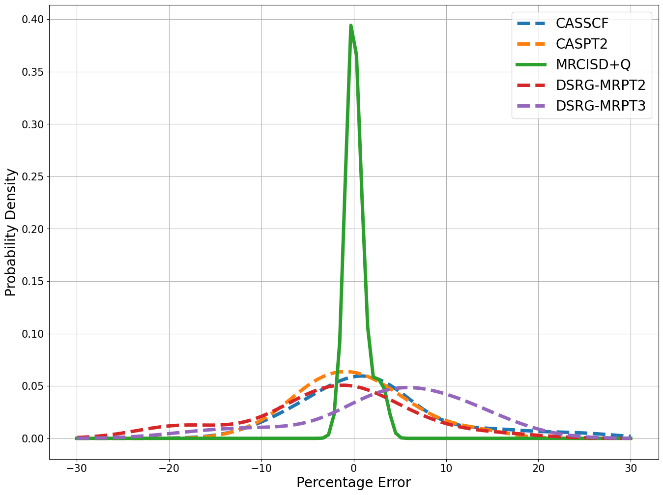
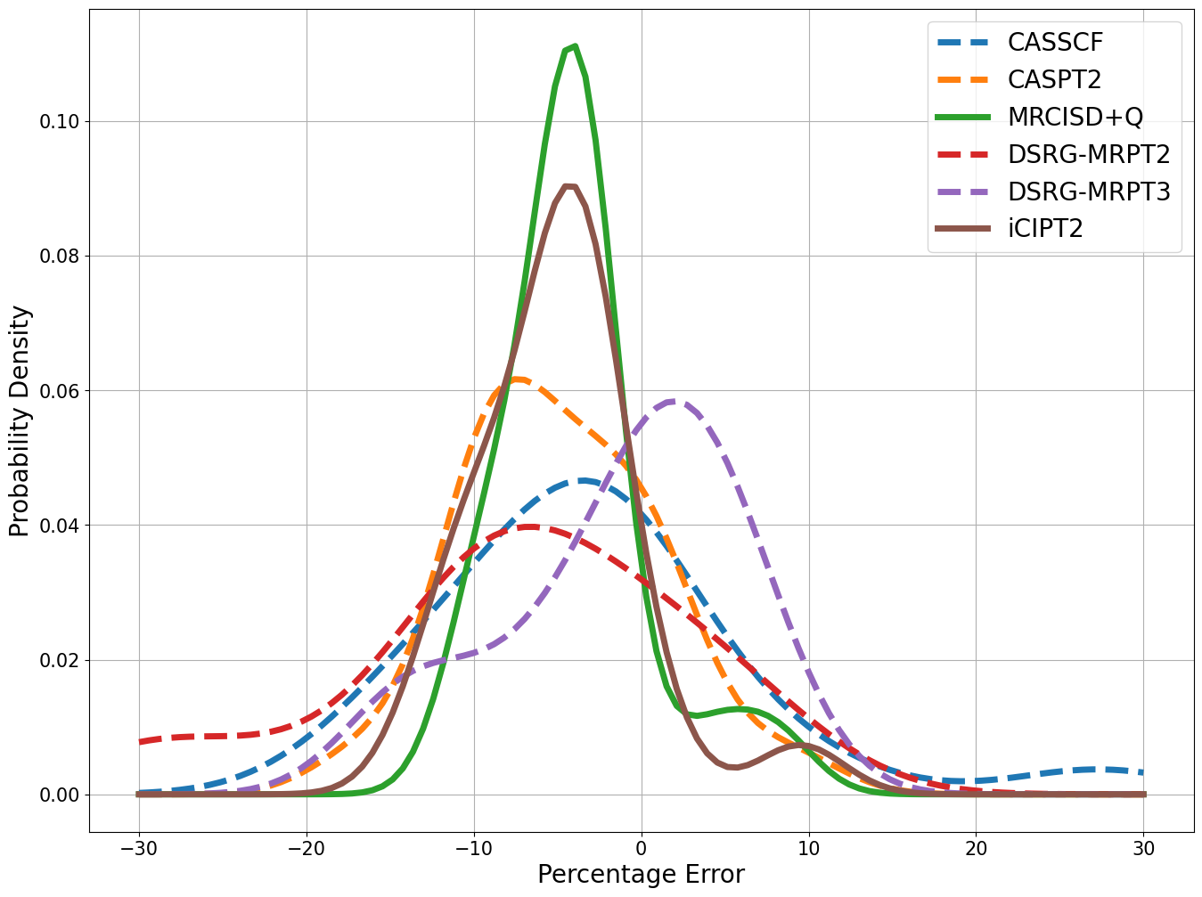
In the present account, it is of more interest to make a close comparison between different methods. To this end, we used the same setup (all-electron correlation with the DCB Hamiltonian and uncontracted cc-pVTZ basis sets142, 143, 133) as in the previous calculations on the selected $p$-block atoms (see Table 4), including 4C-CASSCF, 4C-CASPT2, and 4C-MRCISD+Q (internally contracted multireference configuration interaction with singles and doubles as well as Davidson corrections) in Ref. 144, as well as the driven similarity renormalization group based second- and third-order multireference perturbation theories (DSRG-MRPT2/MRPT3) in Ref. 32. Since the present 4C-iCIPT2 is nearly exact, it should be taken as benchmark to calibrate the other methods. As can be seen from Table 4 and Fig. 5, 4C-MRCISD+Q is closest to 4C-iCIPT2. Yet, DSRG-MRPT3 appears to be closest to experiment (cf. Fig. 6). However, this should not be taken seriously, for the cc-pVTZ basis sets are not sufficiently large, even though uncontracted. As a matter of fact, it was already noticed long ago145 that some tight $p$-functions have to be added to the cc-pVTZ basis sets for more accurate descriptions of the SOSs, especially of the second-row atoms. We therefore repeated the calculations on \ceB to \ceF by using the tight $p$-functions suggested in Ref. 32. As can be seen from Table 5, the SOSs of \ceB to \ceF are indeed improved discernibly with such augmented basis sets. Still, however, even larger basis sets are required to obtain converged results, e.g., the uncontracted cc-pV5Z basis sets142 further reduce the MAPE by more than 2%. As an additional indicator for the request on new basis sets for spinor-based relativistic calculations, we mention that the ordering of the ${}^{3}\text{P}_{2}$, ${}^{3}\text{P}_{0}$, and ${}^{3}\text{P}_{1}$ states of \ceTe could not be reproduced correctly with all the considered basis sets, except for the fortuitous case of valance-only correlation with the scalar relativistically contracted ANO-RCC basis set136 (see Table S4).

Table 4: Comparison between different methods for the spin-orbit splittings (in cm-1) of selected $p$-block atoms with the DCB Hamiltonian and uncontracted cc-pVTZ basis sets142, 143, 133, 134. All electrons were correlated for second-row atoms. Only valence electrons were correlated for third- and fourth-row atoms
atom splitting Expt. CASSCF CASPT2 MRCISD+Q DSRG-MRPT2 DSRG-MRPT3 4C-iCIPT2
B ${}^{2}\text{P}_{1/2}\rightarrow$ ${}^{2}\text{P}_{3/2}$ 15.29 13.25 13.99 13.91 13.99 14.32 13.97
C ${}^{3}\text{P}_{0}\rightarrow$ ${}^{3}\text{P}_{1}$ 16.42 14.94 14.93 15.40 14.93 17.20 15.61
${}^{3}\text{P}_{1}\rightarrow$ ${}^{3}\text{P}_{2}$ 27.00 23.82 23.95 24.88 28.48 28.72 24.61
N ${}^{4}\text{S}_{3/2}\rightarrow$ ${}^{2}\text{D}_{5/2}$ 19224.46 22910.28 20414.63 20095.77a 20231.34 19952.54 20183.94a
${}^{2}\text{D}_{5/2}\rightarrow$ ${}^{2}\text{D}_{3/2}$ 8.71 11.09 9.47 9.40a 9.41 7.89 9.54a
O ${}^{3}\text{P}_{2}\rightarrow$ ${}^{3}\text{P}_{1}$ 158.27 153.24 145.35 152.52 145.35 138.92 152.08
${}^{3}\text{P}_{1}\rightarrow$ ${}^{3}\text{P}_{0}$ 68.71 66.99 62.55 65.85 54.49 58.32 66.12
F ${}^{2}\text{P}_{3/2}\rightarrow$ ${}^{2}\text{P}_{1/2}$ 404.14 382.59 384.70 388.38 384.70 391.68 387.66
Al ${}^{2}\text{P}_{1/2}\rightarrow$ ${}^{2}\text{P}_{3/2}$ 112.06 96.81 106.60 106.96 106.70 108.35 106.43
Si ${}^{3}\text{P}_{0}\rightarrow$ ${}^{3}\text{P}_{1}$ 77.12 72.89 78.90 73.76 69.94 81.52 73.80
${}^{3}\text{P}_{1}\rightarrow$ ${}^{3}\text{P}_{2}$ 146.04 138.28 133.25 140.43 149.20 154.03 140.35
P ${}^{4}\text{S}_{3/2}\rightarrow$ ${}^{2}\text{D}_{3/2}$ 11361.02 15305.18 12561.03 N/A 13302.41 12666.93 12308.90
${}^{2}\text{D}_{3/2}\rightarrow$ ${}^{2}\text{D}_{5/2}$ 15.61 15.34 14.01 N/A 11.08 13.38 13.62
S ${}^{3}\text{P}_{2}\rightarrow$ ${}^{3}\text{P}_{1}$ 396.06 398.64 386.02 383.94 355.94 400.61 386.11
${}^{3}\text{P}_{1}\rightarrow$ ${}^{3}\text{P}_{0}$ 177.59 180.62 161.92 173.46 175.36 181.66 174.36
Cl ${}^{2}\text{P}_{3/2}\rightarrow$ ${}^{2}\text{P}_{1/2}$ 882.35 886.86 894.86 861.80 867.69 888.44 864.17
Ga ${}^{2}\text{P}_{1/2}\rightarrow$ ${}^{2}\text{P}_{3/2}$ 826.19 685.92 776.51 745.97 743.28 791.62 739.16
Ge ${}^{3}\text{P}_{0}\rightarrow$ ${}^{3}\text{P}_{1}$ 557.13 512.35 553.07 502.94b 485.56 570.25 504.81
${}^{3}\text{P}_{1}\rightarrow$ ${}^{3}\text{P}_{2}$ 852.83 809.65 711.39 814.20b 857.09 878.13 795.11
As ${}^{4}\text{S}_{3/2}\rightarrow$ ${}^{2}\text{D}_{3/2}$ 10592.50 14289.54 11799.71 N/A 12567.66 12034.45 11444.25
${}^{2}\text{D}_{3/2}\rightarrow$ ${}^{2}\text{D}_{5/2}$ 322.10 354.53 324.93 N/A 227.88 327.81 285.05
Se ${}^{3}\text{P}_{2}\rightarrow$ ${}^{3}\text{P}_{1}$ 1989.50 1949.63 1917.35 1900.34b 1745.74 1991.36 1886.09
${}^{3}\text{P}_{1}\rightarrow$ ${}^{3}\text{P}_{0}$ 544.86 572.88 532.84 566.74b 573.81 590.89 548.63
Br ${}^{2}\text{P}_{3/2}\rightarrow$ ${}^{2}\text{P}_{1/2}$ 3685.24 3683.62 3704.50 3540.14 3546.46 3683.90 3548.41
MAEc - 19.29 19.35 26.82f 37.77 9.88 26.51
MAPEd - 7.09 6.15 5.24f 9.38 5.24 5.90
MAPEe - 5.36 4.39 0.76f 6.09 7.87 -
  • a

    Two core spinors ($1s_{1/2}$) were frozen for nitrogen. Otherwise, the symmetry breaking, small though, renders the state assignment difficult.

  • b

    Uncontracted cc-pVDZ basis set.

  • c

    Mean absolute error compared to experimental values137 (${}^{4}\text{S}_{3/2}\rightarrow$ ${}^{2}\text{D}_{5/2}$/${}^{2}\text{D}_{3/2}$ of \ceN, \ceP, and \ceAs were excluded).

  • d

    Mean absolute percentage error compared to experimental values137 (${}^{4}\text{S}_{3/2}\rightarrow$ ${}^{2}\text{D}_{5/2}$/${}^{2}\text{D}_{3/2}$ of \ceN, \ceP, and \ceAs were excluded).

  • e

    Mean absolute percentage error compared to 4C-iCIPT2 results (${}^{4}\text{S}_{3/2}\rightarrow$ ${}^{2}\text{D}_{5/2}$/${}^{2}\text{D}_{3/2}$ of \ceN, \ceP, and \ceAs were excluded).

  • f

    Unavailable data were omitted from the averaging.

Table 5: Spin-orbit splittings (in cm-1) and percentage error for the second-row elements with the original (orig.) uncontracted cc-pVTZ basis and the augmented (aug.) sets with a tight $p$-function (68.8243, 106.9535, 152.2273, 196.9866, and 250.83491 for \ceB, \ceC, \ceN, \ceO, and \ceF, respectively. ).
Atom Transition DSRG-MRPT2 DSRG-MRPT3 4C-iCIPT2 Exp.
orig. aug. orig. aug. orig. aug. 5Z orig.a
B ${}^{2}\text{P}_{1/2}\rightarrow$ ${}^{2}\text{P}_{3/2}$ 13.99 (-8.5) 14.81 (-3.1) 14.32 (-6.3) 14.88 (-2.7) 13.97 (-8.6) 14.43 (-5.6) 14.96 (-2.1) 15.29
C ${}^{3}\text{P}_{0}\rightarrow$ ${}^{3}\text{P}_{1}$ 14.93 (-9.1) 17.51 (6.6) 17.20 (4.8) 17.75 (8.1) 15.61 (-4.9) 16.68 (1.6) 16.12 (-1.8) 16.42
${}^{3}\text{P}_{1}\rightarrow$ ${}^{3}\text{P}_{2}$ 28.48 (5.5) 29.56 (9.5) 28.72 (6.4) 29.81 (10.4) 24.61 (-8.9) 24.67 (-8.6) 26.58 (-1.6) 27.00
Nb ${}^{4}\text{S}_{3/2}\rightarrow$ ${}^{2}\text{D}_{5/2}$ 20231.34 (5.2) 20235.14 (5.3) 19952.54 (3.8) 19956.74 (3.8) 20183.94 (5.0) 20187.97 (5.0) 19356.79 (0.7) 19224.46
${}^{2}\text{D}_{5/2}\rightarrow$ ${}^{2}\text{D}_{3/2}$ 9.41 (8.0) 8.02 (-7.9) 7.89 (-9.4) 7.73 (-11.3) 9.54 (9.5) 9.44 (8.4) 8.83 (1.4) 8.71
O ${}^{3}\text{P}_{2}\rightarrow$ ${}^{3}\text{P}_{1}$ 145.35 (-8.2) 133.37 (-15.7) 138.92 (-12.2) 142.57 (-9.9) 152.08 (-3.9) 156.00 (-1.4) 153.69 (2.9) 158.27
${}^{3}\text{P}_{1}\rightarrow$ ${}^{3}\text{P}_{0}$ 54.49 (-20.7) 56.12 (-18.3) 58.32 (-15.1) 60.07 (-12.6) 66.12 (-3.8) 68.25 (-0.7) 68.70 (0.0) 68.71
F ${}^{2}\text{P}_{3/2}\rightarrow$ ${}^{2}\text{P}_{1/2}$ 384.70 (-4.8) 391.15 (-3.2) 391.68 (-3.1) 403.10 (-0.4s) 387.66 (-4.1) 398.81 (-1.3) 399.73 (-1.1) 404.14
MAXc 20.7 18.3 15.1 12.6 9.5 8.6 2.9
MAPEd 9.3 9.2 8.2 7.9 6.2 4.0 1.6
  • a

    Original uncontracted cc-pV5Z (see also Table S1).

  • b

    Two core spinors ($1s_{1/2}$) were frozen in 4C-iCIPT2 calculations of nitrogen. Otherwise, the symmetry breaking, small though, renders the state assignment difficult.

  • c

    Maximal percentage error compared to experimental values137 (${}^{4}\text{S}_{3/2}\rightarrow$ ${}^{2}\text{D}_{5/2}$ of \ceN was excluded).

  • d

    Mean absolute percentage error compared to experimental values137 (${}^{4}\text{S}_{3/2}\rightarrow$ ${}^{2}\text{D}_{5/2}$ of \ceN was excluded).

Refer to caption
Figure 5: Distribution of percentage errors of spin-orbit splittings of selected $p$-block atoms with the DCB Hamiltonian and uncontracted cc-pVTZ basis sets compared to 4C-iCIPT2 results (see Table 4). Probability density was estimated via kernel density estimation using Gaussian kernel. The ${}^{4}\text{S}_{3/2}\rightarrow$ ${}^{2}\text{D}_{5/2}$/${}^{2}\text{D}_{3/2}$ transitions of \ceN, \ceP, and \ceAs were excluded.
Refer to caption
Figure 6: Distribution of percentage errors of spin-orbit splittings of selected $p$-block atoms with the DCB Hamiltonian and uncontracted cc-pVTZ basis sets compared to experimental results137 (see Table 4). Probability density was estimated via kernel density estimation using Gaussian kernel. The ${}^{4}\text{S}_{3/2}\rightarrow$ ${}^{2}\text{D}_{5/2}$/${}^{2}\text{D}_{3/2}$ transitions of \ceN, \ceP, and \ceAs were excluded.

5 CONCLUSIONS and OUTLOOK

It has been shown that relativistic (spin-dependent) wave function methods can straightforwardly be implemented on top of the templates used for their nonrelativistic (spin-free) counterparts by leveraging the power of meta-programming furnished by C++, provided that the same diagrammatical representation is employed for the spin-dependent and spin-free Hamiltonians. For the case of 4C-iCIPT2 considered here, once the code for constructing the Hamiltonian matrix is made ready, all the rest can be generated automatically from the existing templates used for the spin-free iCIPT2. Moreover, both time reversal and binary double point group symmetries can readily be incorporated, so as to facilitate not only the computation but also the state assignment. Although the $p$-block atoms taken here as showcases are not sufficient to reveal the real efficacy of the near-exact 4C-iCIPT2, it is undoubted that 4C-iCIPT2 is applicable to more complex systems containing heavy atoms. Noticeably, the transformation of 4C two-electron integrals from the atomic to molecular orbital representation is awfully expensive and memory intensive. This can be surmounted by going to the picture change-free Q4C Hamiltonian118, 119, where the integral transformation can be performed as a whole instead of component-wise as in the 4C case112. Just like that iCISCF146 results from the use of iCIPT2 as the CI solver of CASSCF and can handle ca. 60 active orbitals, 4C-iCISCF for large active spaces can readily be formulated by taking 4C-iCIPT2 as the CI solver of 4C-CASSCF. Guess orbials can here be provided by the recently proposed Kramers restricted open-shell DHF112. Work along these directions is being carried out at our laboratory.

Acknowledgments

This work was supported by the National Natural Science Foundation of China (Grant No. 22373057) and Mount Tai Scholar Climbing Project of Shandong Province.

Data Availability Statement

The data that support the findings of this study are available within the article.

Conflicts of interest

There are no conflicts to declare.

Appendix A Symmetry in Molecular Integrals

A.1 Time reversal and permutation

Apart from the four-fold permutation symmetries

$\displaystyle(pq|rs)$ $\displaystyle=(rs|pq)=(qp|sr)^{*}=(sr|qp)^{*},\quad p,q,r,s\in A,B,$ (58)
$\displaystyle(p\bm{\alpha}q|r\bm{\alpha}s)$ $\displaystyle=(r\bm{\alpha}s|p\bm{\alpha}q)=(q\bm{\alpha}p|s\bm{\alpha}r)^{*}=(s\bm{\alpha}r|q\bm{\alpha}p)^{*},\quad p,q,r,s\in A,B,$ (59)

the Coulomb and Gaunt/Breit types of ERIs also have the following time reversal-based relations

$\displaystyle(pq|rs)$ $\displaystyle=(pq|\bar{s}\bar{r})=(\bar{q}\bar{p}|rs)=(\bar{q}\bar{p}|\bar{s}\bar{r}),\quad p,q,r,s\in A;\bar{p},\bar{q},\bar{r},\bar{s}\in B,$
$\displaystyle(pq|r\bar{s})$ $\displaystyle=-(pq|s\bar{r})=(\bar{q}\bar{p}|r\bar{s})=-(\bar{q}\bar{p}|s\bar{r}),$
$\displaystyle(p\bar{q}|r\bar{s})$ $\displaystyle=-(p\bar{q}|s\bar{r})=-(q\bar{p}|r\bar{s})=(q\bar{p}|s\bar{r}),$
$\displaystyle(\bar{p}q|r\bar{s})$ $\displaystyle=-(\bar{p}q|s\bar{r})=-(\bar{q}p|r\bar{s})=(\bar{q}p|s\bar{r}),$ (60)
$\displaystyle(p\bm{\alpha}q|r\bm{\alpha}s)$ $\displaystyle=-(p\bm{\alpha}q|\bar{s}\bm{\alpha}\bar{r})=-(\bar{q}\bm{\alpha}\bar{p}|r\bm{\alpha}s)=(\bar{q}\bm{\alpha}\bar{p}|\bar{s}\bm{\alpha}\bar{r}),$
$\displaystyle(p\bm{\alpha}q|r\bm{\alpha}\bar{s})$ $\displaystyle=(p\bm{\alpha}q|s\bm{\alpha}\bar{r})=-(\bar{q}\bm{\alpha}\bar{p}|r\bm{\alpha}\bar{s})=-(\bar{q}\bm{\alpha}\bar{p}|s\bm{\alpha}\bar{r}),$
$\displaystyle(p\bm{\alpha}\bar{q}|r\bm{\alpha}\bar{s})$ $\displaystyle=(p\bm{\alpha}\bar{q}|s\bm{\alpha}\bar{r})=(q\bm{\alpha}\bar{p}|r\bm{\alpha}\bar{s})=(q\bm{\alpha}\bar{p}|s\bm{\alpha}\bar{r}),$
$\displaystyle(\bar{p}\bm{\alpha}q|r\bm{\alpha}\bar{s})$ $\displaystyle=(\bar{p}\bm{\alpha}q|s\bm{\alpha}\bar{r})=(\bar{q}\bm{\alpha}p|r\bm{\alpha}\bar{s})=(\bar{q}\bm{\alpha}p|s\bm{\alpha}\bar{r}),$ (61)

thanks to the following identities

$\displaystyle\psi_{p}^{\dagger}\psi_{q}$ $\displaystyle=\psi_{\bar{q}}^{\dagger}\psi_{\bar{p}},\quad\psi_{\bar{p}}^{\dagger}\psi_{q}=-\psi_{\bar{q}}^{\dagger}\psi_{p},\quad\psi_{p}^{\dagger}\psi_{\bar{q}}=-\psi_{q}^{\dagger}\psi_{\bar{p}},$ (62)
$\displaystyle\psi_{p}^{\dagger}\bm{\alpha}\psi_{q}$ $\displaystyle=-\psi_{\bar{q}}^{\dagger}\bm{\alpha}\psi_{\bar{p}},\quad\psi_{\bar{p}}^{\dagger}\bm{\alpha}\psi_{q}=\psi_{\bar{q}}^{\dagger}\bm{\alpha}\psi_{p},\quad\psi_{p}^{\dagger}\bm{\alpha}\psi_{\bar{q}}=\psi_{q}^{\dagger}\bm{\alpha}\psi_{\bar{p}}.$ (63)

Eq. (60)/(61) allows one to classify the 16-fold ERIs $(pq|rs)_{p,q,r,s\in A,B}$/$(p\bm{\alpha}q|r\bm{\alpha}s)_{p,q,r,s\in A,B}$ into four unique groups,

  1. (1)

    $G_{AAAA}=\{(AA|AA),(AA|BB),(BB|AA),(BB|BB)\}$,

  2. (2)

    $G_{ABBA}=\{(AB|BA),(BA|AB)\}$,

  3. (3)

    $G_{AAAB}=\{(AA|AB),(BA|AA),(AB|AA),(AA|BA),(AB|BB),(BA|BB),(AB|BB),(BB|BA)\}$,

  4. (4)

    $G_{ABAB}=\{(AB|AB),(BA|BA)\}$.

Within each group, the other types of ERIs can all be transformed to the first one . Therefore, only the four generic $(AA|AA)$, $(AB|BA)$, $(AA|AB)$, and $(AB|AB)$ types of ERIs need to be stored. This already gives rise to a four-times reduction of the store, as compared to the storage of the whole 16-fold ERIs. For the $(AA|AA)$ type of ERIs $(pq|rs)$, the four-fold permutation (i.e., $p\geq r$ and $p\geq q$), which covers all the four cases in $G_{AAAA}$, gives rise to a further four-times reduction and hence an overall 16-times reduction of the storage. For the $(AB|BA)$ type of ERIs $(p\bar{q}|\bar{r}s)$ [$=(\bar{r}s|p\bar{q})]$, which have a two-fold permutation (i.e., $p\geq r$) and are anti-symmetric with respect to both the $p,q$ and $r,s$ pairs, an eight-times reduction of the storage can be achieved. Further considering the fact that the group $G_{ABBA}$ has a two-in-one feature, an overall sixteen-times reduction of the storage can be achieved. The type $(AB|AB)$ of ERIs behaves the same as $(AB|BA)$. As for the $(AA|AB)$ type of ERIs $(pq|r\bar{s})$, which have no permutation symmetries but are anti-symmetric with respect to the $r,s$ pair, a two-times reduction of the storage can be achieved. Further considering the fact that the group $G_{AAAB}$ has an eight-in-one feature, again an overall sixteen-times reduction of the storage can be achieved. Therefore, an overall sixteen-times reduction of the storage of the Coulomb/Breit ERIs can be achieved by making use only of time reversal and permutation symmetries.

As noted before123, both the $(AA|AA)$ and $(AB|BA)$ types of ERIs appear in the main diagonal blocks, whereas the $(AA|AB)$ and $(AB|AB)$ types of ERIs enter the first and second off-diagonal blocks, respectively, of the block pentadiagonal Hamiltonian matrix over SDs that are ordered in a descent order of their $M_{K}$ values. It will be shown in Sec. A.2 that the $(AA|AB)$ type of ERIs vanishes for binary double point groups other than $C_{1}^{\ast}$ and $C_{i}^{\ast}$, and that all the ERIs are real-valued for the $C_{2v}^{\ast}$, $D_{2}^{\ast}$, and $D_{2h}^{\ast}$ groups.

A.2 Double Group Symmetry

Suppose a spinor $\psi$ and its time-reversed partner $\bar{\psi}$ transform as the basis of an irreducible representation (irrep) of a binary double point group ($D_{2h}^{\ast}$ and its subgroups), which can be ascribed to one of three Frobenius–Schur classes: (a) $C_{1}^{\ast}$ and $C_{i}^{\ast}$, where $\psi$ and $\bar{\psi}$ belong to the same, non-degenerate fermion irrep; (b) $C_{2}^{\ast}$, $C_{s}^{\ast}$, and $C_{2h}^{\ast}$, where $\psi$ and $\bar{\psi}$ belong to different, non-degenerate fermion irreps (which together form a doubly degenerate fermion representation); (c) $C_{2v}^{\ast}$, $D_{2}^{\ast}$, and $D_{2h}^{\ast}$, where $\psi$ and $\bar{\psi}$ belong to the first and second columns of a doubly degenerate irrep. Such Kramers paired symmetry functions can readily be constructed (even for any double point group)147, so as to render the matrices of Hermitian operators well structured (quaternion, complex, or real for the three Frobenius–Schur classes, respectively). However, the point of focus here is to uncover the distribution of boson irreps of binary double point groups among the individual components of the already symmetrized spinor $\psi$,

$$\psi=\left(\begin{array}[]{l}\psi^{L\alpha}\\ \psi^{L\beta}\\ \psi^{S\alpha}\\ \psi^{S\beta}\end{array}\right)=\left(\begin{array}[]{l}\operatorname{Re}\left(\psi^{L\alpha}\right)+\mathbbm{i}\operatorname{Im}\left(\psi^{L\alpha}\right)\\ \operatorname{Re}\left(\psi^{L\beta}\right)+\mathbbm{i}\operatorname{Im}\left(\psi^{L\beta}\right)\\ \operatorname{Re}\left(\psi^{S\alpha}\right)+\mathbbm{i}\operatorname{Im}\left(\psi^{S\alpha}\right)\\ \operatorname{Re}\left(\psi^{S\beta}\right)+\mathbbm{i}\operatorname{Im}\left(\psi^{S\beta}\right)\\ \end{array}\right).$$ (64)

To this end, we rewrite the one-electron Dirac equation as

$\displaystyle\psi^{L}$ $\displaystyle=\frac{c}{E-V}(\bm{\sigma}\cdot\mathbf{p})B(E)(\bm{\sigma}\cdot\mathbf{p})\psi^{L},$ (65)
$\displaystyle\psi^{S}$ $\displaystyle=B(E)(\bm{\sigma}\cdot\mathbf{p})\psi^{L},$ (66)
$\displaystyle B(E)$ $\displaystyle=\frac{c}{2c^{2}+E-V},$ (67)

where the potential $V$ and hence the operator $B(E)$ are totally symmetric. The $(\bm{\sigma}\cdot\mathbf{p})B(E)(\bm{\sigma}\cdot\mathbf{p})$ operator can further be written in block form

$\displaystyle(\bm{\sigma}\cdot\mathbf{p})B(E)(\bm{\sigma}\cdot\mathbf{p})$ $\displaystyle=\left(\begin{array}[]{cc}\mathbf{p}B(E)\cdot\mathbf{p}+\mathbbm{i}L_{z}&L_{y}+\mathbbm{i}L_{x}\\ -L_{y}+\mathbbm{i}L_{x}&\mathbf{p}B(E)\cdot\mathbf{p}-\mathbbm{i}L_{z}\end{array}\right),$ (70)
$\displaystyle L_{i}$ $\displaystyle=(\mathbf{p}B(E)\times\mathbf{p})_{i},\quad i=x,y,z,$ (71)

where $\mathbf{p}B(E)\cdot\mathbf{p}$ transforms as $r^{2}$ and hence spans the totally symmetric irrep $\Gamma_{0}$, whereas $L_{i}$ is the $i$-th component of the angular momentum and transforms as the rotation $R_{i}$, thereby leading to

$$\Gamma\left((\bm{\sigma}\cdot\mathbf{p})B(E)(\bm{\sigma}\cdot\mathbf{p})\right)=\left(\begin{array}[]{cc}\Gamma_{0}+\mathbbm{i}\Gamma\left(R_{z}\right)&\Gamma\left(R_{y}\right)+\mathbbm{i}\Gamma\left(R_{x}\right)\\ \Gamma\left(R_{y}\right)+\mathbbm{i}\Gamma\left(R_{x}\right)&\Gamma_{0}+\mathbbm{i}\Gamma\left(R_{z}\right)\end{array}\right).$$ (72)

Note that the negative signs in Eq. (70) are immaterial for the symmetry issue. To reveal the symmetry of Eq. (65), we start with a spinor (64) with only $\operatorname{Re}\left(\psi^{L\alpha}\right)$ nonzero, so as to obtain

$\displaystyle\Gamma\left(\psi^{L}\right)$ $\displaystyle=\left(\begin{array}[]{c}\Gamma\left(\operatorname{Re}\psi^{L\alpha}\right)+\mathbbm{i}\Gamma\left(\operatorname{Im}\psi^{L\alpha}\right)\\ \Gamma\left(\operatorname{Re}\psi^{L\beta}\right)+\mathbbm{i}\Gamma\left(\operatorname{Im}\psi^{L\beta}\right)\end{array}\right)$ (75)
$\displaystyle=\left(\begin{array}[]{c}\Gamma_{0}+\mathbbm{i}\Gamma\left(R_{z}\right)\\ \Gamma\left(R_{y}\right)+\mathbbm{i}\Gamma\left(R_{x}\right)\end{array}\right)\otimes\Gamma\left(\operatorname{Re}\psi^{L\alpha}\right).$ (78)

Note that the explicit appearance of imaginary $\mathbbm{i}$ emphasizes the symmetry of the imaginary part of $\psi^{L}$. By virtue of the following identities (cf. Table 6)

$\displaystyle\Gamma\left(R_{i}\right)\otimes\Gamma\left(R_{j}\right)=\Gamma\left(R_{k}\right),\quad(i,j,k)=(x,y,z),$
$\displaystyle\Gamma\left(R_{i}\right)\otimes\Gamma\left(R_{i}\right)=\Gamma_{0},\quad i=x,y,z,$
$\displaystyle\sum_{i=x,y,z}\Gamma(i)\otimes\Gamma\left(R_{i}\right)=\Gamma(\mathbf{r}\cdot\mathbf{R}),$ (79)

it can readily be checked that the repeated application of the operator (72) on $\Gamma\left(\psi^{L}\right)$ (78) does not change the result. Therefore, Eq. (78) does reveal the full internal symmetry structure of the large component $\psi^{L}$.

To reveal the internal symmetry structure of the small component $\psi^{S}$, we invoke the symmetry content of the $\bm{\sigma}\cdot\mathbf{p}$ operator, viz.,

$$\Gamma(\bm{\sigma}\cdot\mathbf{p})=\left(\begin{array}[]{cc}\mathbbm{i}\Gamma(z)&\Gamma(y)+\mathbbm{i}\Gamma(x)\\ \Gamma(y)+\mathbbm{i}\Gamma(x)&\mathbbm{i}\Gamma(z)\end{array}\right).$$ (80)

Multiplying $\Gamma(\bm{\sigma}\cdot\mathbf{p})$ from the left of Eq. (78) gives rise to

$\displaystyle\Gamma\left(\psi^{S}\right)$ $\displaystyle=\left(\begin{array}[]{cc}\mathbbm{i}\Gamma(z)&\Gamma(y)+\mathbbm{i}\Gamma(x)\\ \Gamma(y)+\mathbbm{i}\Gamma(x)&\mathbbm{i}\Gamma(z)\end{array}\right)\left(\begin{array}[]{c}\Gamma_{0}+\mathbbm{i}\Gamma\left(R_{z}\right)\\ \Gamma\left(R_{y}\right)+\mathbbm{i}\Gamma\left(R_{x}\right)\end{array}\right)\otimes\Gamma\left(\operatorname{Re}\psi^{L\alpha}\right)$ (85)
$\displaystyle=\left(\begin{array}[]{cc}\Gamma(\mathbf{r}\cdot\mathbf{R})\left[\Gamma_{0}+\mathbbm{i}\Gamma\left(R_{z}\right)\right]\\ \Gamma(\mathbf{r}\cdot\mathbf{R})\left[\Gamma\left(R_{y}\right)+\mathbbm{i}\Gamma\left(R_{x}\right)\right]\end{array}\right)\otimes\Gamma\left(\operatorname{Re}\psi^{L\alpha}\right)$ (88)
$\displaystyle=\Gamma(\mathbf{r}\cdot\mathbf{R})\otimes\Gamma\left(\psi^{L}\right)$ (89)

in view of Eq. (66) and the identities in Eq. (79). It follows from Eqs. (78) and (89) that the boson irreps of the eight scalar functions in $\psi$ (cf. Eq. (64)) are not independent, but are determined148, 123 solely by $\Gamma\left(\operatorname{Re}\psi^{L\alpha}\right)$, the irrep of the real part of the $L\alpha$ component. In particular, the small component $\psi^{S}$ differs from the large component $\psi^{L}$ only in parity (because $\mathbf{r}\cdot\mathbf{R}$ changes sign under spatial inversion).

Given the internal symmetry structure of $\psi$, that of the time-reversed partner $\bar{\psi}$ can be obtained simply by interchanging the boson irreps of the $\alpha$ and $\beta$ components of $\psi^{X}$ ($X=L,S$), viz.,

$\displaystyle\Gamma\left(\bar{\psi}^{L}\right)$ $\displaystyle=\left(\begin{array}[]{c}\Gamma\left(\operatorname{Re}\psi^{L\beta}\right)+\mathbbm{i}\Gamma\left(\operatorname{Im}\psi^{L\beta}\right)\\ \Gamma\left(\operatorname{Re}\psi^{L\alpha}\right)+\mathbbm{i}\Gamma\left(\operatorname{Im}\psi^{L\alpha}\right)\end{array}\right)$ (92)
$\displaystyle=\left(\begin{array}[]{c}\Gamma\left(R_{y}\right)+\mathbbm{i}\Gamma\left(R_{x}\right)\\ \Gamma_{0}+\mathbbm{i}\Gamma\left(R_{z}\right)\\ \end{array}\right)\otimes\Gamma\left(\operatorname{Re}\psi^{L\alpha}\right),$ (95)
$\displaystyle\Gamma\left(\bar{\psi}^{S}\right)$ $\displaystyle=\Gamma(\mathbf{r}\cdot\mathbf{R})\otimes\Gamma\left(\bar{\psi}^{L}\right).$ (96)

With the above relations, the binary boson irreps for the components of spinors $\psi$ and $\bar{\psi}$ (of a given Frobenius–Schur class) can readily be generated when $\Gamma\left(\operatorname{Re}\psi^{L\alpha}\right)$ is chosen to be the totally symmetric irrep $\Gamma_{0}$, see Tables 7-9. However, the spatial inversion has not yet been taken into account. As such, the procedure should be repeated for $C_{i}^{\ast}$, $C_{2h}^{\ast}$, and $D_{2h}^{\ast}$ by setting $\Gamma\left(\operatorname{Re}\psi^{L\alpha}\right)$ to the totally anti-symmetric irrep $A_{u}$, so as to complete the lists for the three groups. As a matter of fact, $\Gamma\left(\operatorname{Re}\psi^{L\alpha}\right)$ can be set to any boson irrep $\Gamma_{b}$ (and its opposite-parity counterpart, if any), with the corresponding distributions of boson irreps being those obtained by multiplying $\Gamma_{b}$ to the ones documented in Tables 7-9. Such information can be employed reversely for the construction of Kramers paired symmetry functions of binary double point groups148.

Table 6: Symmetry of operators connecting the small and large components.
double group $(\Gamma(x),\Gamma(y),\Gamma(z))$ $(\Gamma(R_{x}),\Gamma(R_{y}),\Gamma(R_{z}))$ $\Gamma(\mathbf{r}\cdot\mathbf{R})$
$C_{1}^{\ast}$ $(A,A,A)$ $(A,A,A)$ $A$
$C_{i}^{\ast}$ $(A_{u},A_{u},A_{u})$ $(A_{g},A_{g},A_{g})$ $A_{u}$
$C_{2}^{\ast}$ $(B,B,A)$ $(B,B,A)$ $A$
$C_{s}^{\ast}$ $(A^{\prime},A^{\prime},A^{\prime\prime})$ $(A^{\prime\prime},A^{\prime\prime},A^{\prime})$ $A^{\prime\prime}$
$C_{2h}^{\ast}$ $(B_{u},B_{u},A_{u})$ $(B_{g},B_{g},A_{g})$ $A_{u}$
$C_{2v}^{\ast}$ $(B_{1},B_{2},A_{1})$ $(B_{2},B_{1},A_{2})$ $A_{2}$
$D_{2}^{\ast}$ $(B_{3},B_{2},B_{1})$ $(B_{3},B_{2},B_{1})$ $A$
$D_{2h}^{\ast}$ $(B_{3u},B_{2u},B_{1u})$ $(B_{3g},B_{2g},B_{1g})$ $A_{u}$
Table 7: Symmetry of each component of spinors $\psi$ and $\bar{\psi}$ for $C_{1}^{\ast}$ and $C_{i}^{\ast}$ (Frobenius-Schur class (a))
$C_{1}^{\ast}$ $C_{i}^{\ast}$
$\psi/\bar{\psi}\in A_{1/2}$ $\psi_{g}/\bar{\psi}_{g}\in A_{1/2,g}$ $\psi_{u}/\bar{\psi}_{u}\in A_{1/2,u}$
$\psi^{L\alpha}$ $A+iA$ $A_{g}+iA_{g}$ $A_{u}+iA_{u}$
$\psi^{L\beta}$ $A+iA$ $A_{g}+iA_{g}$ $A_{u}+iA_{u}$
$\psi^{S\alpha}$ $A+iA$ $A_{u}+iA_{u}$ $A_{g}+iA_{g}$
$\psi^{S\beta}$ $A+iA$ $A_{u}+iA_{u}$ $A_{g}+iA_{g}$
Table 8: Symmetry of each component of spinors $\psi$ and $\bar{\psi}$ for $C_{2}^{\ast}$, $C_{s}^{\ast}$ and $C_{2h}^{\ast}$ (Frobenius-Schur class (b))
$C_{2}^{\ast}$ $C_{s}^{\ast}$ $C_{2h}^{\ast}$
$\psi\in$ ${}^{1}E_{1/2}$ $\bar{\psi}\in$ ${}^{2}E_{1/2}$ $\psi\in$ ${}^{1}E_{1/2}$ $\bar{\psi}\in$ ${}^{2}E_{1/2}$ $\psi_{g}\in$ ${}^{1}E_{1/2,g}$ $\bar{\psi}_{g}\in$ ${}^{2}E_{1/2,g}$ $\psi_{u}\in$ ${}^{1}E_{1/2,u}$ $\bar{\psi}_{u}\in$ ${}^{2}E_{1/2,u}$
$\psi^{L\alpha}$ $A+iA$ $B+iB$ $A^{\prime}+iA^{\prime}$ $A^{\prime\prime}+iA^{\prime\prime}$ $A_{g}+iA_{g}$ $B_{g}+iB_{g}$ $A_{u}+iA_{u}$ $B_{u}+iB_{u}$
$\psi^{L\beta}$ $B+iB$ $A+iA$ $A^{\prime\prime}+iA^{\prime\prime}$ $A^{\prime}+iA^{\prime}$ $B_{g}+iB_{g}$ $A_{g}+iA_{g}$ $B_{u}+iB_{u}$ $A_{u}+iA_{u}$
$\psi^{S\alpha}$ $A+iA$ $B+iB$ $A^{\prime\prime}+iA^{\prime\prime}$ $A^{\prime}+iA^{\prime}$ $A_{u}+iA_{u}$ $B_{u}+iB_{u}$ $A_{g}+iA_{g}$ $B_{g}+iB_{g}$
$\psi^{S\beta}$ $B+iB$ $A+iA$ $A^{\prime}+iA^{\prime}$ $A^{\prime\prime}+iA^{\prime\prime}$ $B_{u}+iB_{u}$ $A_{u}+iA_{u}$ $B_{g}+iB_{g}$ $A_{g}+iA_{g}$
Table 9: Symmetry of each component of spinors $\psi$ and $\bar{\psi}$ for $C_{2v}^{\ast}$, $D_{2}^{\ast}$ and $D_{2h}^{\ast}$ (Frobenius-Schur class (c))
$C_{2v}^{\ast}$ $D_{2}^{\ast}$ $D_{2h}^{\ast}$
$(\psi,\bar{\psi})\in E_{1/2}$ $(\psi,\bar{\psi})\in E_{1/2}$ $(\psi_{g},\bar{\psi}_{g})\in E_{1/2,g}$ $(\psi_{u},\bar{\psi}_{u})\in E_{1/2,u}$
$\psi^{L\alpha}$ $(A_{1}+iA_{2},B_{1}+iB_{2})$ $(A+iB_{1},B_{2}+iB_{3})$ $(A_{g}+iB_{1g},B_{2g}+iB_{3g})$ $(A_{u}+iB_{1u},B_{2u}+iB_{3u})$
$\psi^{L\beta}$ $(B_{1}+iB_{2},A_{1}+iA_{2})$ $(B_{2}+iB_{3},A+iB_{1})$ $(B_{2g}+iB_{3g},A_{g}+iB_{1g})$ $(B_{2u}+iB_{3u},A_{u}+iB_{1u})$
$\psi^{S\alpha}$ $(A_{2}+iA_{1},B_{2}+iB_{1})$ $(A+iB_{1},B_{2}+iB_{3})$ $(A_{u}+iB_{1u},B_{2u}+iB_{3u})$ $(A_{g}+iB_{1g},B_{2g}+iB_{3g})$
$\psi^{S\beta}$ $(B_{2}+iB_{1},A_{2}+iA_{1})$ $(B_{2}+iB_{3},A+iB_{1})$ $(B_{2u}+iB_{3u},A_{u}+iB_{1u})$ $(B_{2g}+iB_{3g},A_{g}+iB_{1g})$

By virtue of the relations (78), (89), (95), (96), and (79), the symmetries of the (scalar) overlap charge density and current density components can readily be calculated as

$\displaystyle\Gamma\left(\psi_{p}^{\dagger}\psi_{q}|_{p,q\in A,B}\right)$ $\displaystyle=\begin{cases}\left[\Gamma_{0}+\mathbbm{i}\Gamma\left(R_{z}\right)\right]\otimes\Gamma_{2LA}\quad(\mbox{even A})\\ \left[\Gamma\left(R_{y}\right)+\mathbbm{i}\Gamma\left(R_{x}\right)\right]\otimes\Gamma_{2LA}\quad(\mbox{odd A})\end{cases},$ (97)
$\displaystyle\Gamma\left(\psi_{p}^{\dagger}\alpha_{x}\psi_{q}|_{p,q\in A,B}\right)$ $\displaystyle=\begin{cases}\Gamma\left(\mathbf{r}\cdot\mathbf{R}\right)\otimes\left[\Gamma\left(R_{y}\right)+\mathbbm{i}\Gamma\left(R_{x}\right)\right]\otimes\Gamma_{2LA}\quad(\mbox{even A})\\ \Gamma\left(\mathbf{r}\cdot\mathbf{R}\right)\otimes\left[\Gamma_{0}+\mathbbm{i}\Gamma\left(R_{z}\right)\right]\otimes\Gamma_{2LA}\quad(\mbox{odd A})\end{cases},$ (98)
$\displaystyle\Gamma\left(\psi_{p}^{\dagger}\alpha_{y}\psi_{q}|_{p,q\in A,B}\right)$ $\displaystyle=\begin{cases}\Gamma\left(\mathbf{r}\cdot\mathbf{R}\right)\otimes\left[\Gamma\left(R_{x}\right)+\mathbbm{i}\Gamma\left(R_{y}\right)\right]\otimes\Gamma_{2LA}\quad(\mbox{even A})\\ \Gamma\left(\mathbf{r}\cdot\mathbf{R}\right)\otimes\left[\Gamma\left(R_{z}\right)+\mathbbm{i}\Gamma_{0}\right]\otimes\Gamma_{2LA}\quad(\mbox{odd A})\end{cases},$ (99)
$\displaystyle\Gamma\left(\psi_{p}^{\dagger}\alpha_{z}\psi_{q}|_{p,q\in A,B}\right)$ $\displaystyle=\begin{cases}\Gamma\left(\mathbf{r}\cdot\mathbf{R}\right)\otimes\left[\Gamma_{0}+\mathbbm{i}\Gamma\left(R_{z}\right)\right]\otimes\Gamma_{2LA}\quad(\mbox{even A})\\ \Gamma\left(\mathbf{r}\cdot\mathbf{R}\right)\otimes\left[\Gamma\left(R_{y}\right)+\mathbbm{i}\Gamma\left(R_{x}\right)\right]\otimes\Gamma_{2LA}\quad(\mbox{odd A})\end{cases},$ (100)

where

$\displaystyle\Gamma_{2LA}$ $\displaystyle=\Gamma\left(\operatorname{Re}\psi^{L\alpha}_{p}\right)\Gamma\left(\operatorname{Re}\psi^{L\alpha}_{q}\right)|_{p,q\in A},$ (101)

and ‘even/odd A’ is a shorthand notation for ‘even/odd number of A spinors’. We then have

$\displaystyle\Gamma\left(\psi_{p}^{\dagger}\psi_{q}\psi_{r}^{\dagger}\psi_{s}|_{p,q,r,s\in A,B}\right)$ $\displaystyle=\Gamma\left(\psi_{p}^{\dagger}\alpha_{i}\psi_{q}\psi_{r}^{\dagger}\alpha_{i}\psi_{s}|_{p,q,r,s\in A,B}\right),\quad i\in x,y,z$
$\displaystyle=\begin{cases}\left[\Gamma_{0}+\mathbbm{i}\Gamma\left(R_{z}\right)\right]\otimes\Gamma_{4LA}\quad(\mbox{even A})\\ \left[\Gamma\left(R_{y}\right)+\mathbbm{i}\Gamma\left(R_{x}\right)\right]\otimes\Gamma_{4LA}\quad(\mbox{odd A})\end{cases},$ (102)

where

$\displaystyle\Gamma_{4LA}$ $\displaystyle=\Gamma\left(\operatorname{Re}\psi^{L\alpha}_{p}\right)\Gamma\left(\operatorname{Re}\psi^{L\alpha}_{q}\right)\Gamma\left(\operatorname{Re}\psi^{L\alpha}_{r}\right)\Gamma\left(\operatorname{Re}\psi^{L\alpha}_{s}\right)|_{p,q,r,s\in A}.$ (103)

It follows that the Coulomb/Gaunt/Breit two-electron repulsion integrals (ERI) have exactly the same point group symmetries and are nonzero only when the real or imaginary part of the quartet $\psi_{p}^{\dagger}\psi_{q}\psi_{r}^{\dagger}\psi_{s}|_{p,q,r,s\in A,B}$ contains the totally symmetric irrep $\Gamma_{0}$. As pointed out previously, all $\{\operatorname{Re}\psi^{L\alpha}_{\cdot}\}$ must be assigned to the same boson irrep (or its opposite-parity counterpart, if any) for internal consistency. Therefore, $\Gamma_{4LA}$ (103) is always equal to $\Gamma_{0}$ [NB: in the presence of spatial inversion as in $C_{i}^{\ast}$, $C_{2h}^{\ast}$, and $D_{2h}^{\ast}$, the number of ungerade $\{\operatorname{Re}\psi^{L\alpha}_{p};p\in A\}$ (equivalently, the number of ungerade A- or B-spinors, for $\psi_{p}$ and $\psi_{\bar{p}}$ have the same parity as $\operatorname{Re}\psi^{L\alpha}_{p}$) in the quartet must be even for nonzero ERIs]. As such, Eq. (102) can actually be simplified to

$\displaystyle\Gamma\left(\psi_{p}^{\dagger}\psi_{q}\psi_{r}^{\dagger}\psi_{s}|_{p,q,r,s\in A,B}\right)$ $\displaystyle=\Gamma\left(\psi_{p}^{\dagger}\alpha_{i}\psi_{q}\psi_{r}^{\dagger}\alpha_{i}\psi_{s}|_{p,q,r,s\in A,B}\right),\quad i\in x,y,z$
$\displaystyle=\begin{cases}\left[\Gamma_{0}+\mathbbm{i}\Gamma\left(R_{z}\right)\right]\quad(\mbox{even A})\\ \left[\Gamma\left(R_{y}\right)+\mathbbm{i}\Gamma\left(R_{x}\right)\right]\quad(\mbox{odd A})\end{cases}.$ (104)

It is then clear that only $C_{1}^{\ast}$ and $C_{i}^{\ast}$ permit both even and odd numbers of A-spinors, for both $\Gamma\left(R_{z}\right)$ and $\Gamma\left(R_{x}\right)$ are equal to $\Gamma_{0}$ in this case. In contrast, $\Gamma\left(R_{x}\right)$ is different from $\Gamma_{0}$ for the other binary double point groups, such that an odd number of A-spinors (or equivalently B-spinors) is not permitted therein. Since $\Gamma\left(R_{z}\right)$ is also equal to $\Gamma_{0}$ for $C_{2}^{\ast}$, $C_{s}^{\ast}$, and $C_{2h}^{\ast}$, the ERIs are complex-valued, just like those of $C_{1}^{\ast}$ and $C_{i}^{\ast}$. On the other hand, $\Gamma\left(R_{z}\right)$ is different from $\Gamma_{0}$ for $C_{2v}^{\ast}$, $D_{2}^{\ast}$, and $D_{2h}^{\ast}$, thereby leading to real-valued ERIs.

In short, we have the following selection rules for the ERIs solely due to symmetry reasons:

  • The Coulomb and Gaunt/Breit ERIs have exactly the same point group symmetries;

  • Except for $C_{1}^{\ast}$ and $C_{i}^{\ast}$, the quartet $\psi_{p}^{\dagger}\psi_{q}\psi_{r}^{\dagger}\psi_{s}|_{p,q,r,s\in A,B}$ must contain an even number of A/B-spinors;

  • For $C_{i}^{\ast}$, $C_{2h}^{\ast}$, and $D_{2h}^{\ast}$, the quartet $\psi_{p}^{\dagger}\psi_{q}\psi_{r}^{\dagger}\psi_{s}|_{p,q,r,s\in A,B}$ must contain an even number of gerade/ungerade spinors;

  • The ERIs are real-valued for $C_{2v}^{\ast}$, $D_{2}^{\ast}$, and $D_{2h}^{\ast}$, but are complex-valued for the other binary double point groups.

Such rules will be employed to construct symmetry-adapted many-electron basis functons in Sec. B. Note in passing that the same analysis can also be performed for the one-electron case: just like $\Gamma_{4LA}$ (103), $\Gamma_{2LA}$ (101) in Eq. (97) must also be the totally symmetric irrep $\Gamma_{0}$ in order for the integrals of totally symmetric one-body operators to be nonzero, thereby leading to the following selection rules:

  • Except for $C_{1}^{\ast}$ and $C_{i}^{\ast}$, the doublet $\psi_{p}^{\dagger}\psi_{q}|_{p,q\in A,B}$ must contain an even number of A/B-spinors;

  • For $C_{i}^{\ast}$, $C_{2h}^{\ast}$, and $D_{2h}^{\ast}$, the doublet $\psi_{p}^{\dagger}\psi_{q}|_{p,q\in A,B}$ must contain an even number of gerade/ungerade spinors;

  • The one-electron integrals are real-valued for $C_{2v}^{\ast}$, $D_{2}^{\ast}$, and $D_{2h}^{\ast}$, but are complex-valued for the other binary double point groups.

Finally, it deserves to be mentioned that all the one- and two-electron integrals discussed so far can actually be made real-valued (for arbitrary double point groups)147. However, this must be companied by proper recombinations of the excitation operators, which complicate the implementation of correlated wave function methods. Nevertheless, this option deserves to be considered in future.

Appendix B Symmetry in Many-Electron Functions

After having discussed extensively the time reversal and double point group symmetries inherent in the relativistic ERIs (see Appendix A), we are ready to discuss the symmetries of MBFs.

B.1 Odd Number of Electrons

For systems of an odd number of electrons, the MBFs are associated to a fermion irrep of the given double point group. When calculating the eigenstates, only one partner of a degenerate Kramers pair needs to be solved, which results in a two-times reduction of the computational cost. This holds irrespective of point group symmetries. As shown in Sec. A.2, for the $C_{2}^{\ast}$, $C_{s}^{\ast}$, $C_{2h}^{\ast}$, $C_{2v}^{\ast}$, $D_{2}^{\ast}$, and $D_{2h}^{\ast}$ groups, the molecular ERIs can be nonzero only when the quartets $\psi_{p}^{\dagger}\psi_{q}\psi_{r}^{\dagger}\psi_{s}|_{p,q,r,s\in A,B}$ contain an even number of B-spinors. For an odd number of electrons, we have $\tilde{M}_{K}=1$ or $3$ for every MBF. The MBFs of different $\tilde{M}_{K}$ values belong to different fermion irreps in the case of $C_{2}^{\ast}$, $C_{s}^{\ast}$, and $C_{2h}^{\ast}$, and to different columns of the same fermion irrep in the case of $C_{2v}^{\ast}$, $D_{2}^{\ast}$, and $D_{2h}^{\ast}$ (cf. Table. B.1). Therefore, the Hamiltonian matrix elements in between are absolutely zero, which results in an additional two-times reduction of the computational cost for these groups. For $C_{2v}^{\ast}$, $D_{2}^{\ast}$, and $D_{2h}^{\ast}$, a further two-times reduction can be gained due to the fact that the Hamiltonian matrix elements are all real-valued. Finally, the spatial inversion in $C_{i}$, $C_{2h}^{\ast}$, and $D_{2h}^{\ast}$ also gives a two-times reduction. Therefore, for systems of an odd number of electrons, the combined use of time reversal and point group symmetries reduces the computational cost by factors of 2, 4, 4, 4, 8, 8, 8, and 16 for the $C_{1}^{\ast}$, $C_{i}$, $C_{2}^{\ast}$, $C_{s}^{\ast}$, $C_{2h}^{\ast}$, $C_{2v}^{\ast}$, $D_{2}^{\ast}$, and $D_{2h}^{\ast}$ point groups, respectively, which are precisely their group orders.

Binary double point group symmetries of $N$-electron basis functions built up with $N_{A}$ A-spinors and $N_{B}$ B-spinors. odd N even N 1a 3a $(0,1)$b $(0,-1)$b $(2,1)$b $(2,-1)$b $C_{1}^{\ast}$ $A_{1/2}$ $A_{1/2}$ $A$ $A$ $A$ $A$ $C_{i}^{\ast}$c $A_{1/2,g}/A_{1/2,u}$ $A_{1/2,g}/A_{1/2,u}$ $A_{g}/A_{u}$ $A_{g}/A_{u}$ $A_{g}/A_{u}$ $A_{g}/A_{u}$ $C_{2}^{\ast}$ ${}^{1}E_{1/2}$ ${}^{2}E_{1/2}$ $A$ $A$ $B$ $B$ $C_{s}^{\ast}$ ${}^{1}E_{1/2}$ ${}^{2}E_{1/2}$ $A^{\prime}$ $A^{\prime}$ $A^{\prime\prime}$ $A^{\prime\prime}$ $C_{2h}^{\ast}$c ${}^{1}E_{1/2,g}/^{1}E_{1/2,u}$ ${}^{2}E_{1/2,g}/^{2}E_{1/2,u}$ $A_{g}/A_{u}$ $A_{g}/A_{u}$ $B_{g}/B_{u}$ $B_{g}/B_{u}$ $C_{2v}^{\ast}$ $E_{1/2,1/2}$ $E_{1/2,-1/2}$ $A_{1}$ $A_{2}$ $B_{1}$ $B_{2}$ $D_{2}^{\ast}$ $E_{1/2,1/2}$ $E_{1/2,-1/2}$ $A$ $B_{1}$ $B_{2}$ $B_{3}$ $D_{2h}^{\ast}$c $E_{1/2,1/2,g}/E_{1/2,1/2,u}$ $E_{1/2,-1/2,g}/E_{1/2,-1/2,u}$ $A_{g}/A_{u}$ $B_{1g}/B_{1u}$ $B_{2g}/B_{2u}$ $B_{3g}/B_{3u}$

  • a

    $\tilde{M}_{K}=(N_{A}-N_{B})\mod 4$. The assignment of $\tilde{M}_{K}=1$ and 3 to the first and second columns of the irrep $E_{1/2}$ of $C_{2v}^{\ast}$, $D_{2}^{\ast}$, and $D_{2}^{\ast}$ is not unambiguous, but which does not affect the computation nor the state assignment.

  • b

    $(\tilde{M}_{K},s)$ with $s=\pm 1$ in Eq. (17).

  • c

    The gerade (g) and ungerade (u) parities are determined automatically by those of the occupied spinors.

B.2 Even Number of Electrons

For systems of an even number of electrons, the MBFs must belong to a boson irrep of the given double binary point group. Since the time reversal-based transformation (17) renders the Hamiltonian matrix elements (18) real-valued, a two-times reduction of the computational cost can always be achieved, irrespective of point group symmetries. Like the case of an odd number of electrons, the quartet $\psi_{p}^{\dagger}\psi_{q}\psi_{r}^{\dagger}\psi_{s}|_{p,q,r,s\in A,B}$ must contain an even number of B-spinors for the $C_{2}^{\ast}$, $C_{s}^{\ast}$, $C_{2h}^{\ast}$, $C_{2v}^{\ast}$, $D_{2}^{\ast}$, and $D_{2h}^{\ast}$ groups. The MBFs of $\tilde{M}_{K}=0$ and 2 are associated to the totally symmetric and the other boson irreps, respectively, in the case of $C_{2}^{\ast}$ and $C_{s}^{\ast}$. This gives rise to an additional two-times reduction, leading to an overall four-times reduction for $C_{2}^{\ast}$ and $C_{s}^{\ast}$. The situation is similar for $C_{2h}^{\ast}$, except that the parity has to be distinguished here (which gives rise to an additional two-times reduction, thereby leading to an overall eight-times reduction). For the $C_{2v}^{\ast}$, $D_{2}^{\ast}$, and $D_{2h}^{\ast}$ groups, which have more than two boson irreps, the two $\tilde{M}_{K}$ values (00 or $2$) are themselves not enough to distinguish the MBFs. Instead, the $s$ values ($=\pm 1$) in Eq. (17) should further be employed (cf. Table. B.1). It turns out that the boson irrep for each $(\tilde{M}_{K},s)$ pair can readily be determined for the case of two electrons, by first calculating the actions of symmetry operations $\hat{R}$ on the fermion basis $(\psi,\bar{\psi})$, viz.,

$$\hat{R}(\psi,\bar{\psi})=(\psi^{\prime},\bar{\psi}^{\prime})=(\psi,\bar{\psi})\mathbf{D}^{(E_{1/2})}(R),$$

where $\{\mathbf{D}^{(E_{1/2})}(R),\forall R\in E_{1/2}\}$ are the matrix representations of the irrep $E_{1/2}$ of $C_{2v}^{\ast}$, $D_{2}^{\ast}$, and $D_{2h}^{\ast}$, and then calculating

$\displaystyle\hat{R}M^{\pm}$ $\displaystyle=c_{\pm}(R)M^{\pm},$
$\displaystyle M^{\pm}$ $\displaystyle\sim\psi_{p}\psi_{q}\pm\psi_{\bar{p}}\psi_{\bar{q}}\quad(\tilde{M}_{K}=2),$
$\displaystyle M^{\pm}$ $\displaystyle\sim\psi_{p}\psi_{\bar{q}}\mp\psi_{\bar{p}}\psi_{q}\quad(\tilde{M}_{K}=0),$

where the coefficients $c_{\pm}(R)$ are just the matrix elements (characters) of a (one-dimensional) boson irrep. It can then be proven by induction that the results are the same for $2m$ ($m>1$) electrons. Together with time reversal, the four $(\tilde{M}_{K},s)$ pairs give rise to an overall eight-times reduction for $C_{2v}^{\ast}$, $D_{2}^{\ast}$, and an overall sixteen-times reduction for $D_{2h}^{\ast}$ (due to parity). In short, for systems of an even number of electrons, the combined use of time reversal and point group symmetries also reduces the computational cost by the orders of the binary double point groups.

Appendix C Special treat of Hamiltonian matrix elements

C.1 Matrix elements $\langle I\mu|H_{1}^{0}+H_{2}^{0}|I\mu\rangle$

The diagonal matrix elements $\langle I\mu|H_{1}^{0}+H_{2}^{0}|I\mu\rangle$ are composed of two terms

$\displaystyle\mathcal{A}^{0}_{1}$ $\displaystyle=\sum_{p}h_{pp}\tilde{n}_{p}+\sum_{p}[(\bar{p}\bar{p}|pp)-(\bar{p}p|p\bar{p})]n_{p}n_{\bar{p}}+\sum_{p<q}(pp|qq)\tilde{n}_{p}\tilde{n}_{q},$ (105)
$\displaystyle\mathcal{A}^{0}_{2}$ $\displaystyle=-\sum_{p<q}\left[(pq|qp)(n_{p}n_{q}+n_{\bar{p}}n_{\bar{q}})+(\bar{p}q|q\bar{p})(n_{\bar{p}}n_{q}+n_{p}n_{\bar{q}})\right],$ (106)

where the summations run over Kramers pairs. A close inspection reveals that $\mathcal{A}^{0}_{1}$ depends only on the PON $\tilde{n}_{p}$, since $n_{p}n_{\bar{p}}$ is non-vanishing if and only if $\tilde{n}_{p}=2$, where $n_{p}=n_{\bar{p}}=1$. On the other hand, if the PON of Kramers pair $\mathcal{P}_{p}$ or $\mathcal{P}_{q}$ is 2, e.g., $\tilde{n}_{p}=2$ and hence $n_{p}=n_{\bar{p}}=1$, $\mathcal{A}^{0}_{2}$ (106) would read

$\displaystyle-(pq|qp)(n_{p}n_{q}+n_{\bar{p}}n_{\bar{q}})-(\bar{p}q|q\bar{p})(n_{\bar{p}}n_{q}+n_{p}n_{\bar{q}})$
$\displaystyle=-(pq|qp)\tilde{n}_{q}-(\bar{p}q|q\bar{p})\tilde{n}_{q}$
$\displaystyle=-[(pq|qp)+(\bar{p}q|q\bar{p})]\tilde{n}_{q},$

which depends only on the PON $\tilde{n}_{q}$. Therefore, $\mathcal{A}^{0}_{2}$ (106) is to be evaluated case by case only when $\tilde{n}_{p}=\tilde{n}_{q}=1$. However, the expressions $\mathcal{A}^{0}_{1}$ (105) and $\mathcal{A}^{0}_{2}$ (106) are not yet optimal, as they are both quadratic with respect to the number of occupied Kramers pairs. The problem can be mitigated109 by introducing a closed-shell reference oCFG $|\omega\rangle$ with $\tilde{\omega}_{p}=\omega_{p}+\omega_{\bar{p}}=2$ or 0 (NB: the total number of electrons is chosen to be $N-1$ for odd $N$). Then, any oCFG $|I\rangle$ can be characterized by the differential occupations $\Delta_{p}=n_{p}^{I}-\omega_{p}$, $\Delta_{\bar{p}}=n_{\bar{p}}^{I}-\omega_{\bar{p}}$, and $\tilde{\Delta}_{p}=\Delta_{p}+\Delta_{\bar{p}}$. The three terms in $\mathcal{A}_{1}^{0}$ (105) can therefore be rewritten, respectively, as

$\displaystyle\sum_{p}h_{pp}(\omega_{p}+\omega_{\bar{p}}+\Delta_{p}+\Delta_{\bar{p}})$ $\displaystyle=\sum_{p}h_{pp}\tilde{\omega}_{p}+h_{pp}(\Delta_{p}+\Delta_{\bar{p}})$
$\displaystyle=\sum_{p}h_{pp}\tilde{\omega}_{p}+h_{pp}\tilde{\Delta}_{p},$ (107)
$\displaystyle\sum_{p}[(\bar{p}\bar{p}|pp)-(\bar{p}p|p\bar{p})]n_{p}n_{\bar{p}}=\sum_{p}[(\bar{p}\bar{p}|pp)-(\bar{p}p|p\bar{p})](\omega_{p}+\Delta_{p})(\omega_{\bar{p}}+\Delta_{\bar{p}})$
$\displaystyle=\sum_{p}[(\bar{p}\bar{p}|pp)-(\bar{p}p|p\bar{p})]\omega_{p}\omega_{\bar{p}}+\sum_{p}[(\bar{p}\bar{p}|pp)-(\bar{p}p|p\bar{p})](\Delta_{p}\omega_{\bar{p}}+\Delta_{\bar{p}}\omega_{p})$
$\displaystyle+\sum_{p}[(\bar{p}\bar{p}|pp)-(\bar{p}p|p\bar{p})]\Delta_{p}\Delta_{\bar{p}}$
$\displaystyle=\sum_{p}[(\bar{p}\bar{p}|pp)-(\bar{p}p|p\bar{p})]\delta_{\tilde{\omega}_{p},2}+\sum_{p}[(\bar{p}\bar{p}|pp)-(\bar{p}p|p\bar{p})]\tilde{\Delta}_{p}\delta_{\tilde{\omega}_{p},2}$
$\displaystyle+\sum_{p}[(\bar{p}\bar{p}|pp)-(\bar{p}p|p\bar{p})][\delta_{\tilde{\Delta}_{p},2}+\delta_{\tilde{\Delta}_{p},-2}],$ (108)
$\displaystyle\sum_{p<q}(pp|qq)\tilde{n}_{p}\tilde{n}_{q}$ $\displaystyle=\sum_{p<q}(pp|qq)(\tilde{\omega}_{p}+\tilde{\Delta}_{p})(\tilde{\omega}_{q}+\tilde{\Delta}_{q})$
$\displaystyle=\sum_{p<q}(pp|qq)(\tilde{\omega}_{p}\tilde{\omega}_{q}+\tilde{\omega}_{p}\tilde{\Delta}_{q}+\tilde{\omega}_{q}\tilde{\Delta}_{p}+\tilde{\Delta}_{p}\tilde{\Delta}_{q})$
$\displaystyle=\sum_{p<q}4(pp|qq)\delta_{\tilde{\omega}_{p},2}\delta_{\tilde{\omega}_{q},2}+\sum_{q}\left\{\sum_{p\neq q}2(pp|qq)\delta_{\tilde{\omega}_{p},2}\right\}\tilde{\Delta}_{q}$
$\displaystyle+\sum_{p<q}(pp|qq)\tilde{\Delta}_{p}\tilde{\Delta}_{q}.$ (109)

Likewise, $\mathcal{A}^{0}_{2}$ (106) can be written as

$\displaystyle\small\mathcal{A}^{0}_{2}=$ $\displaystyle-\sum_{p<q}\left\{(pq|qp)\left[(\omega_{p}+\Delta_{p})(\omega_{q}+\Delta_{q})+(\omega_{\bar{p}}+\Delta_{\bar{p}})(\omega_{\bar{q}}+\Delta_{\bar{q}})\right]\right.$
$\displaystyle+\left.(\bar{p}q|q\bar{p})\left[(\omega_{\bar{p}}+\Delta_{\bar{p}})(\omega_{q}+\Delta_{q})+(\omega_{p}+\Delta_{p})(\omega_{\bar{q}}+\Delta_{\bar{q}})\right]\right\}$
$\displaystyle=$ $\displaystyle-\sum_{p<q}\left\{(pq|qp)\left[\omega_{p}\omega_{q}+\omega_{\bar{p}}\omega_{\bar{q}}\right]+(\bar{p}q|q\bar{p})\left[\omega_{\bar{p}}\omega_{q}+\omega_{p}\omega_{\bar{q}}\right]\right\}$
$\displaystyle-$ $\displaystyle\sum_{p<q}(pq|qp)\left[\omega_{p}\Delta_{q}+\omega_{q}\Delta_{p}+\omega_{\bar{p}}\Delta_{\bar{q}}+\omega_{\bar{q}}\Delta_{\bar{p}}\right]$
$\displaystyle-$ $\displaystyle\sum_{p<q}(\bar{p}q|q\bar{p})\left[\omega_{p}\Delta_{\bar{q}}+\omega_{\bar{p}}\Delta_{q}+\omega_{\bar{q}}\Delta_{p}+\omega_{q}\Delta_{\bar{p}}\right]$
$\displaystyle-$ $\displaystyle\sum_{p<q}\left\{(pq|qp)\left[\Delta_{p}\Delta_{q}+\Delta_{\bar{p}}\Delta_{\bar{q}}\right]+(\bar{p}q|q\bar{p})\left[\Delta_{\bar{p}}\Delta_{q}+\Delta_{p}\Delta_{\bar{q}}\right]\right\}$
$\displaystyle=$ $\displaystyle-2\sum_{p<q}\left\{(pq|qp)\delta_{\tilde{\omega}_{p},2}\delta_{\tilde{\omega}_{q},2}+(\bar{p}q|q\bar{p})\delta_{\tilde{\omega}_{p},2}\delta_{\tilde{\omega}_{q},2}\right\}$
$\displaystyle-$ $\displaystyle\sum_{p<q}[(pq|qp)+(\bar{p}q|q\bar{p})]\left[\delta_{\tilde{\omega}_{p},2}\tilde{\Delta}_{q}+\delta_{\tilde{\omega}_{q},2}\tilde{\Delta}_{p}\right]$
$\displaystyle-$ $\displaystyle\sum_{p<q}\left\{(pq|qp)\left[\Delta_{p}\Delta_{q}+\Delta_{\bar{p}}\Delta_{\bar{q}}\right]+(\bar{p}q|q\bar{p})\left[\Delta_{\bar{p}}\Delta_{q}+\Delta_{p}\Delta_{\bar{q}}\right]\right\}$
$\displaystyle=$ $\displaystyle-2\sum_{p<q}\left[(pq|qp)+(\bar{p}q|q\bar{p})\right]\delta_{\tilde{\omega}_{p},2}\delta_{\tilde{\omega}_{q},2}-\sum_{q\neq p}\left[(pq|qp)+(\bar{p}q|q\bar{p})\right]\delta_{\tilde{\omega}_{q},2}\tilde{\Delta}_{p}$
$\displaystyle-$ $\displaystyle\sum_{p<q}\left\{(pq|qp)\left[\Delta_{p}\Delta_{q}+\Delta_{\bar{p}}\Delta_{\bar{q}}\right]+(\bar{p}q|q\bar{p})\left[\Delta_{\bar{p}}\Delta_{q}+\Delta_{p}\Delta_{\bar{q}}\right]\right\}.$ (110)

Here, it is to be noted that if one of the Kramers pairs, say $\mathcal{P}_{q}$, satisfies $\tilde{\Delta}_{q}=\pm 2$ (i.e., $\Delta_{q}=\Delta_{\bar{q}}=\pm 1$), then both $\Delta_{p}\Delta_{q}+\Delta_{\bar{p}}\Delta_{\bar{q}}$ and $\Delta_{\bar{p}}\Delta_{q}+\Delta_{p}\Delta_{\bar{q}}$ are equal to $\pm\tilde{\Delta}_{p}$. Therefore, Eq. (110) can be reorganized to

$\displaystyle\small\mathcal{A}^{0}_{2}=$ $\displaystyle-2\sum_{p<q}\left[(pq|qp)+(\bar{p}q|q\bar{p})\right]\delta_{\tilde{\omega}_{p},2}\delta_{\tilde{\omega}_{q},2}-\sum_{q\neq p}\left[(pq|qp)+(\bar{p}q|q\bar{p})\right]\delta_{\tilde{\omega}_{q},2}\tilde{\Delta}_{p}$
$\displaystyle-\sum_{p\neq q}[(pq|qp)+(\bar{p}q|q\bar{p})]\delta_{\tilde{\Delta}_{p},2}\tilde{\Delta}_{q}+\sum_{p\neq q}[(pq|qp)+(\bar{p}q|q\bar{p})]\delta_{\tilde{\Delta}_{p},-2}\tilde{\Delta}_{q}$
$\displaystyle-\sum_{p<q}^{\prime}\left\{(pq|qp)\left[\Delta_{p}\Delta_{q}+\Delta_{\bar{p}}\Delta_{\bar{q}}\right]+(\bar{p}q|q\bar{p})\left[\Delta_{\bar{p}}\Delta_{q}+\Delta_{p}\Delta_{\bar{q}}\right]\right\},$ (111)

where $\sum^{\prime}$ indicates that both Kramers pairs $\mathcal{P}_{p}$ and $\mathcal{P}_{q}$ are singly occupied. $\mathcal{A}^{0}_{2}$ (111) can be combined with $\mathcal{A}_{1}^{0}$ (107)–(109) to yield the final expression for $H^{0}_{\text{D}}=\mathcal{A}^{0}_{1}+\mathcal{A}^{0}_{2}$ in Eq. (46). In most cases, only a few Kramers pairs possess non-zero $\Delta_{p}$ or $\Delta_{\bar{p}}$, thereby simplifying the evaluation of the diagonal matrix elements significantly.

C.2 Matrix Elements $\langle I\mu|H_{1}^{1}+H_{2}^{1}|J\nu\rangle$

When an oCFG $|I\rangle$ can be obtained from oCFG $|J\rangle$ by exciting a single electron from spinor $q_{\tau}$ to $p_{\sigma}$ ($\neq q_{\tau}$), the matrix elements of the first term of $H_{2}^{1}$ (32) (denoted as $H_{2,\mathrm{c}}^{1}$) read

$\displaystyle\langle I\mu|H_{2,\mathrm{c}}^{1}|J\nu\rangle$ $\displaystyle=\left[(p_{\sigma}q_{\tau}|p_{\bar{\sigma}}p_{\bar{\sigma}})n_{p_{\bar{\sigma}}}^{J\nu}+(p_{\sigma}q_{\tau}|q_{\bar{\tau}}q_{\bar{\tau}})n^{J\nu}_{q_{\bar{\tau}}}\right]\gamma^{I\mu,J\nu}_{p_{\sigma}q_{\tau}}.$ (112)

The matrix elements of the first, direct term in the second term of $H_{2}^{1}$ (32) (denoted as $H_{2,\mathrm{d}}^{1}$), along with $H_{1}^{1}$ (26), take the following form

$\displaystyle\langle I\mu|H_{1}^{1}+H_{2,\mathrm{d}}^{1}|J\nu\rangle$ $\displaystyle=[h_{p_{\sigma}q_{\tau}}+\sum_{\lambda}\sum_{r}^{\prime}(p_{\sigma}q_{\tau}|r_{\lambda}r_{\lambda})n^{J\nu}_{r_{\lambda}}]\gamma^{I\mu,J\nu}_{p_{\sigma}q_{\tau}}$
$\displaystyle=[h_{p_{\sigma}q_{\tau}}+\sum_{r}^{\prime}(p_{\sigma}q_{\tau}|rr)\tilde{n}^{J}_{r}]\gamma^{I\mu,J\nu}_{p_{\sigma}q_{\tau}},$ (113)

where use of the relation $(p_{\sigma}q_{\tau}|rr)=(p_{\sigma}q_{\tau}|\bar{r}\bar{r})$ has been made to arrive at the second equality, and the summation $\sum^{\prime}_{r}$ over Kramers pair excludes $r=p$ or $q$. Taking the common closed-shell oCFG as the reference (i.e., $\tilde{n}_{r}^{J}=\tilde{\omega}_{r}+\tilde{\Delta}_{r}^{J}$), Eq. (113) can further be written as

$\displaystyle\langle I\mu|H_{1}^{1}+H_{2,\mathrm{d}}^{1}|J\nu\rangle$ $\displaystyle=[f^{\mathrm{c}}_{p_{\sigma}q_{\tau}}+\sum_{r}^{\prime}(p_{\sigma}q_{\tau}|rr)\tilde{\Delta}_{r}^{J}]\gamma^{I\mu,J\nu}_{p_{\sigma}q_{\tau}},$ (114)
$\displaystyle f^{\mathrm{c}}_{p_{\sigma}q_{\tau}}$ $\displaystyle=h_{p_{\sigma}q_{\tau}}+2\sum_{r}^{\prime}(p_{\sigma}q_{\tau}|rr)\delta_{\tilde{\omega}_{r},2},$ (115)

where $f^{\mathrm{c}}_{p_{\sigma}q_{\tau}}$ depends only on the closed-shell reference oCFG.

The matrix elements of the second, exchange term in the second term of $H_{2}^{1}$ (32) (denoted as $H_{2,\mathrm{e}}^{1}$) read

$\displaystyle\langle I\mu|H_{2,\mathrm{e}}^{1}|J\nu\rangle$ $\displaystyle=\sum_{r}^{\prime}(p_{\sigma}r|rq_{\tau})\Gamma_{p_{\sigma}rrq_{\tau}}^{I\mu J\nu}+(p_{\sigma}\bar{r}|\bar{r}q_{\tau})\Gamma_{p_{\sigma}\bar{r}\bar{r}q_{\tau}}^{I\mu J\nu}$
$\displaystyle+(p_{\sigma}r|\bar{r}q_{\tau})\Gamma_{p_{\sigma}r\bar{r}q_{\tau}}^{I\mu J\nu}+(p_{\sigma}\bar{r}|rq_{\tau})\Gamma_{p_{\sigma}\bar{r}rq_{\tau}}^{I\mu J\nu}$
$\displaystyle=$ $\displaystyle-\sum_{\lambda}\sum_{r}^{\prime}(p_{\sigma}r_{\lambda}|r_{\lambda}q_{\tau})n_{r_{\lambda}}^{J\nu}\gamma_{p_{\sigma}q_{\tau}}^{I\mu J\nu}+\sum_{\lambda}\sum_{r}^{\prime}(p_{\sigma}r_{\lambda}|r_{\bar{\lambda}}q_{\tau})\Gamma_{p_{\sigma}r\bar{r}q_{\tau}}^{I\mu J\nu}$
$\displaystyle=$ $\displaystyle-\sum_{\lambda}\sum_{r}^{\prime}(p_{\sigma}r_{\lambda}|r_{\lambda}q_{\tau})\delta_{\tilde{n}_{r},2}\gamma_{p_{\sigma}q_{\tau}}^{I\mu J\nu}-\sum_{\lambda}\sum_{r}^{\prime}(p_{\sigma}r_{\lambda}|r_{\lambda}q_{\tau})\delta_{\tilde{n}_{r},1}n_{r_{\lambda}}\gamma_{p_{\sigma}q_{\tau}}^{I\mu J\nu}$
$\displaystyle+\sum_{\lambda}\sum_{r}^{\prime}(p_{\sigma}r_{\lambda}|r_{\bar{\lambda}}q_{\tau})\Gamma_{p_{\sigma}r\bar{r}q_{\tau}}^{I\mu J\nu},$ (116)

which can be combined with Eqs. (112) and (113) to yield the final expression (51).

C.3 Matrix elements of the Gaunt/Breit interaction

Since the Gaunt/Breit ERIs differ formally from the Coulomb ERIs only in time reversal symmetry (cf. Eqs. (61) and (60)), the same procedures as adopted in Appendices C.1 and C.2 can be adopted to derive the corresponding matrix elements.

The diagonal term for the matrix elements between SDs of the same oCFG $|I\rangle$ reads

$\displaystyle H^{0,\mathrm{G}}_{\text{D}}$ $\displaystyle=E^{\mathrm{G}}_{\mathrm{ref}}+\left\{\sum_{p}[(\bar{p}\bm{\alpha}\bar{p}|p\bm{\alpha}p)-(\bar{p}\bm{\alpha}p|p\bm{\alpha}\bar{p})]\tilde{\Delta}_{p}\delta_{\tilde{\omega}_{p},2}\right.$
$\displaystyle\left.+\sum_{p}[(\bar{p}\bm{\alpha}\bar{p}|p\bm{\alpha}p)-(\bar{p}\bm{\alpha}p|p\bm{\alpha}\bar{p})][\delta_{\tilde{\Delta}_{p},2}+\delta_{\tilde{\Delta}_{p},-2}]\right\}$
$\displaystyle-\sum_{q}\tilde{\Delta}_{q}\sum_{p\neq q}[(p\bm{\alpha}q|q\bm{\alpha}p)+(\bar{p}\bm{\alpha}q|q\bm{\alpha}\bar{p})]\delta_{\tilde{\omega}_{p},2}$
$\displaystyle-\sum_{p\neq q}[(p\bm{\alpha}q|q\bm{\alpha}p)+(\bar{p}\bm{\alpha}q|q\bm{\alpha}\bar{p})]\tilde{\Delta}_{p}\delta_{\tilde{\Delta}_{q},2}$
$\displaystyle+\sum_{p\neq q}[(p\bm{\alpha}q|q\bm{\alpha}p)+(\bar{p}\bm{\alpha}q|q\bm{\alpha}\bar{p})]\tilde{\Delta}_{p}\delta_{\tilde{\Delta}_{q},-2}$
$\displaystyle-\sum_{p<q}^{\prime}\left\{(p\bm{\alpha}q|q\bm{\alpha}p)\left[\Delta_{p}\Delta_{q}+\Delta_{\bar{p}}\Delta_{\bar{q}}\right]+(\bar{p}\bm{\alpha}q|q\bm{\alpha}\bar{p})\left[\Delta_{\bar{p}}\Delta_{q}+\Delta_{p}\Delta_{\bar{q}}\right]\right\}$
$\displaystyle+\sum_{p<q}^{\prime}(p\bm{\alpha}p|\bm{\alpha}q)(n_{p}-n_{\bar{p}})(n_{q}-n_{\bar{q}}),$ (117)

where the summations run over Kramers pairs and $\sum^{\prime}$ means that both Kramers pairs $\mathcal{P}_{p}$ and $\mathcal{P}_{q}$ are singly occupied. The reference energy $E_{\mathrm{ref}}^{\mathrm{G}}$ reads

$\displaystyle E_{\mathrm{ref}}^{\mathrm{G}}$ $\displaystyle=\sum_{p}[(p\bm{\alpha}p|\bar{p}\bm{\alpha}\bar{p})-(p\bm{\alpha}\bar{p}|\bar{p}\bm{\alpha}p)]\delta_{\tilde{\omega}_{p},2}$
$\displaystyle-\sum_{p<q}2[(p\bm{\alpha}q|q\bm{\alpha}p)+(\bar{p}\bm{\alpha}q|q\bm{\alpha}\bar{p})]\delta_{\tilde{\omega}_{p},2}\delta_{\tilde{\omega}_{q},2}.$ (118)

The off-diagonal matrix elements take the following form

$\displaystyle\langle I\mu|H_{\mathrm{O}}^{0,\mathrm{G}}|I\nu\rangle$ $\displaystyle=\sum_{p<q}[(\bar{p}\bm{\alpha}p|\bar{q}\bm{\alpha}q)-(\bar{p}\bm{\alpha}q|\bar{q}\bm{\alpha}p)]\Gamma^{I\mu I\nu}_{\bar{p}p,\bar{q}q}$
$\displaystyle+\sum_{p<q}[(\bar{p}\bm{\alpha}p|q\bm{\alpha}\bar{q})-(\bar{p}\bm{\alpha}\bar{q}|q\bm{\alpha}p)]\Gamma^{I\mu I\nu}_{\bar{p}p,q\bar{q}}$
$\displaystyle+\sum_{p<q}[(p\bm{\alpha}\bar{p}|\bar{q}\bm{\alpha}q)-(p\bm{\alpha}q|\bar{q}\bm{\alpha}\bar{p})]\Gamma^{I\mu I\nu}_{p\bar{p},\bar{q}q}$
$\displaystyle+\sum_{p<q}[(p\bm{\alpha}\bar{p}|q\bm{\alpha}\bar{q})-(p\bm{\alpha}\bar{q}|q\bm{\alpha}\bar{p})]\Gamma^{I\mu I\nu}_{p\bar{p},q\bar{q}}$
$\displaystyle-\sum_{p<q}[(\bar{p}\bm{\alpha}q|q\bm{\alpha}p)-(\bar{p}\bm{\alpha}p|q\bm{\alpha}q)](n_{q}-n_{\bar{q}})\gamma^{I\mu I\nu}_{\bar{p}p}$
$\displaystyle-\sum_{p<q}[(p\bm{\alpha}\bar{q}|q\bm{\alpha}p)-(p\bm{\alpha}p|q\bm{\alpha}\bar{q})](n_{p}-n_{\bar{p}})\gamma^{I\mu I\nu}_{q\bar{q}}$
$\displaystyle-\sum_{p<q}[(p\bm{\alpha}q|\bar{q}\bm{\alpha}p)-(p\bm{\alpha}p|\bar{q}\bm{\alpha}q)](n_{p}-n_{\bar{p}})\gamma^{I\mu I\nu}_{\bar{q}q}$
$\displaystyle-\sum_{p<q}[(p\bm{\alpha}q|q\bm{\alpha}\bar{p})-(p\bm{\alpha}\bar{p}|q\bm{\alpha}q)](n_{q}-n_{\bar{q}})\gamma^{I\mu I\nu}_{p\bar{p}}.$ (119)

When an SD $|I\mu\rangle$ can be obtained from $|J\nu\rangle$ by exciting a single electron from spinor $q_{\tau}$ to $p_{\sigma}$ ($\neq q_{\tau}$), we have

$\displaystyle\langle I\mu|H_{1}^{1,\mathrm{G}}+H_{2}^{1,\mathrm{G}}|J\nu\rangle$ $\displaystyle=\left\{(p_{\sigma}\bm{\alpha}q_{\tau}|p_{\bar{\sigma}}\bm{\alpha}p_{\bar{\sigma}})n_{p_{\bar{\sigma}}}^{J\nu}+(p_{\sigma}\bm{\alpha}q_{\tau}|q_{\bar{\tau}}\bm{\alpha}q_{\bar{\tau}})n_{q_{\bar{\tau}}}^{J\nu}\right.$
$\displaystyle\left.-\sum_{\lambda}\sum_{r}^{\prime}(p_{\sigma}\bm{\alpha}r_{\lambda}|r_{\lambda}\bm{\alpha}q_{\tau})n_{r_{\lambda}}^{J\nu}\right\}\gamma^{I\mu J\nu}_{p_{\sigma}q_{\tau}}$
$\displaystyle+\sum_{\lambda}\sum_{r}^{\prime}[(p_{\sigma}\bm{\alpha}r_{\lambda}|r_{\bar{\lambda}}\bm{\alpha}q_{\tau})-(p_{\sigma}s\bm{\alpha}q_{\tau}|r_{\bar{\lambda}}\bm{\alpha}r_{\lambda})]\Gamma_{p_{\sigma}r_{\lambda},r_{\bar{\lambda}}q_{\tau}}^{I\mu J\nu}$
$\displaystyle+\sum_{r}^{\prime}(p_{\sigma}\bm{\alpha}q_{\tau}|r\bm{\alpha}r)(n_{r}^{J\nu}-n_{\bar{r}}^{J\nu})\gamma^{I\mu J\nu}_{p_{\sigma}q_{\tau}},$ (120)

where the summation $\sum_{r}^{\prime}$ over Kramers pairs excludes $r=p$ or $q$. All the terms need to be calculated only for Kramers pairs with different PONs or those that are commonly singly occupied.

Finally, for the case of double excitations, we have

$\displaystyle\langle I\mu|H_{2}^{2,\mathrm{G}}|J\nu\rangle$ $\displaystyle=\left[2^{-\delta_{p_{\sigma}r_{\lambda}}\delta_{q_{\tau}s_{\delta}}}(p_{\sigma}\bm{\alpha}q_{\tau}|r_{\lambda}\bm{\alpha}s_{\delta})\right.$
$\displaystyle\left.-(1-\delta_{p_{\sigma}r_{\lambda}})(1-\delta_{q_{\tau}s_{\delta}})(p_{\sigma}\bm{\alpha}s_{\delta}|r_{\lambda}\bm{\alpha}q_{\tau})\right]\Gamma_{p_{\sigma}q_{\tau},r_{\lambda}s_{\delta}}^{I\mu J\nu}.$ (121)

References

  • Liu 2023 Liu, W. Perspective: Simultaneous treatment of relativity, correlation, and QED. WIRES Comput. Mol. Sci. 2023, 13, e1652
  • Niskanen et al. 2017 Niskanen, J.; Jänkälä, K.; Huttula, M.; Föhlisch, A. QED effects in 1s and 2s single and double ionization potentials of the noble gases. J. Chem. Phys. 2017, 146, 144312
  • Pašteka et al. 2017 Pašteka, L. F.; Eliav, E.; Borschevsky, A.; Kaldor, U.; Schwerdtfeger, P. Relativistic coupled cluster calculations with variational quantum electrodynamics resolve the discrepancy between experiment and theory concerning the electron affinity and ionization potential of gold. Phys. Rev. Lett. 2017, 118, 023002
  • Sunaga et al. 2022 Sunaga, A.; Salman, M.; Saue, T. 4-component relativistic Hamiltonian with effective QED potentials for molecular calculations. J. Chem. Phys. 2022, 157, 164101
  • Liu and Lindgren 2013 Liu, W.; Lindgren, I. Going beyond “no-pair relativistic quantum chemistry”. J. Chem. Phys. 2013, 139, 014108, (E)144, 049901 (2016).
  • Liu 2014 Liu, W. Advances in relativistic molecular quantum mechanics. Phys. Rep. 2014, 537, 59–89
  • Liu 2014 Liu, W. Perspective: relativistic hamiltonians. Int. J. Quantum Chem. 2014, 114, 983–986
  • Liu 2015 Liu, W. Effective quantum electrodynamics Hamiltonians: a tutorial review. Int. J. Quantum Chem. 2015, 115, 631–640, (E)116, 971 (2016).
  • Liu 2016 Liu, W. Big picture of relativistic molecular quantum mechanics. Natl. Sci. Rev. 2016, 3, 204–221
  • Liu 2020 Liu, W. Essentials of relativistic quantum chemistry. J. Chem. Phys. 2020, 152, 180901
  • Liu 2020 Liu, W. Relativistic quantum chemistry: today and tomorrow. Sci. Sin. Chim. 2020, 50, 1672–1696
  • Kutzelnigg 2012 Kutzelnigg, W. Solved and unsolved problems in relativistic quantum chemistry. Chem. Phys. 2012, 395, 16–34
  • Liu 2012 Liu, W. Perspectives of relativistic quantum chemistry: the negative energy cat smiles. Phys. Chem. Chem. Phys. 2012, 14, 35–48
  • Li et al. 2012 Li, Z.; Shao, S.; Liu, W. Relativistic explicit correlation: Coalescence conditions and practical suggestions. J. Chem. Phys. 2012, 136, 144117
  • Jeszenszki et al. 2021 Jeszenszki, P.; Ferenc, D.; Mátyus, E. All-order explicitly correlated relativistic computations for atoms and molecules. J. Chem. Phys. 2021, 154, 224110
  • Jeszenszki et al. 2022 Jeszenszki, P.; Ferenc, D.; Mátyus, E. Variational Dirac–Coulomb explicitly correlated computations for atoms and molecules. J. Chem. Phys. 2022, 156, 084111
  • Hollósy et al. 2024 Hollósy, P.; Jeszenszki, P.; Mátyus, E. One-particle operator representation over two-particle basis sets for relativistic QED computations. J. Chem. Theory Comput. 2024, 20, 5122–5132
  • Jørgen Aa. Jensen et al. 1996 Jørgen Aa. Jensen, H.; Dyall, K. G.; Saue, T.; Fægri Jr, K. Relativistic four-component multiconfigurational self-consistent-field theory for molecules: Formalism. J. Chem. Phys. 1996, 104, 4083–4097
  • Fleig et al. 1997 Fleig, T.; Marian, C. M.; Olsen, J. Spinor optimization for a relativistic spin-dependent CASSCF program. Theor. Chem. Acc. 1997, 97, 125–135
  • Kim and Lee 2003 Kim, Y. S.; Lee, Y. S. The Kramers’ restricted complete active space self-consistent-field method for two-component molecular spinors and relativistic effective core potentials including spin–orbit interactions. J. Chem. Phys. 2003, 119, 12169–12178
  • Kim and Lee 2013 Kim, I.; Lee, Y. S. Two-component Kramers restricted complete active space self-consistent field method with relativistic effective core potential revisited: Theory, implementation, and applications to spin-orbit splitting of lower p-block atoms. J. Chem. Phys. 2013, 139, 134115
  • Thyssen et al. 2008 Thyssen, J.; Fleig, T.; Jensen, H. J. A. A direct relativistic four-component multiconfiguration self-consistent-field method for molecules. J. Chem. Phys. 2008, 129, 034109
  • Bates and Shiozaki 2015 Bates, J. E.; Shiozaki, T. Fully relativistic complete active space self-consistent field for large molecules: Quasi-second-order minimax optimization. J. Chem. Phys. 2015, 142, 044112
  • Reynolds et al. 2018 Reynolds, R. D.; Yanai, T.; Shiozaki, T. Large-scale relativistic complete active space self-consistent field with robust convergence. J. Chem. Phys. 2018, 149, 014106
  • Jenkins et al. 2019 Jenkins, A. J.; Liu, H.; Kasper, J. M.; Frisch, M. J.; Li, X. Variational Relativistic Two-Component Complete-Active-Space Self-Consistent Field Method. J. Chem. Theory Comput. 2019, 15, 2974–2982
  • Dyall 1994 Dyall, K. G. Second-order Møller-Plesset perturbation theory for molecular Dirac-Hartree-Fock wavefunctions. Theory for up to two open-shell electrons. Chem. Phys. Lett. 1994, 224, 186–194
  • Vilkas et al. 1999 Vilkas, M. J.; Ishikawa, Y.; Koc, K. Relativistic multireference many-body perturbation theory for quasidegenerate systems: Energy levels of ions of the oxygen isoelectronic sequence. Phys. Rev. A 1999, 60, 2808
  • Abe et al. 2006 Abe, M.; Nakajima, T.; Hirao, K. The relativistic complete active-space second-order perturbation theory with the four-component Dirac Hamiltonian. J. Chem. Phys. 2006, 125, 234110
  • Kim and Lee 2014 Kim, I.; Lee, Y. S. Two-component multi-configurational second-order perturbation theory with Kramers restricted complete active space self-consistent field reference function and spin-orbit relativistic effective core potential. J. Chem. Phys. 2014, 141, 164104
  • Shiozaki and Mizukami 2015 Shiozaki, T.; Mizukami, W. Relativistic internally contracted multireference electron correlation methods. J. Chem. Theory Comput. 2015, 11, 4733–4739
  • Lu et al. 2022 Lu, L.; Hu, H.; Jenkins, A. J.; Li, X. Exact-two-component relativistic multireference second-order perturbation theory. J. Chem. Theory Comput. 2022, 18, 2983–2992
  • Zhao and Evangelista 2024 Zhao, Z.; Evangelista, F. A. Toward Accurate Spin–Orbit Splittings from Relativistic Multireference Electronic Structure Theory. J. Phys. Chem. Lett. 2024, 15, 7103–7110
  • Visscher et al. 1995 Visscher, L.; Dyall, K. G.; Lee, T. J. Kramers-restricted closed-shell ccsd theory. Int. J. Quantum Chem. 1995, 56, 411–419
  • Visscher et al. 1996 Visscher, L.; Lee, T. J.; Dyall, K. G. Formulation and implementation of a relativistic unrestricted coupled-cluster method including noniterative connected triples. J. Chem. Phys. 1996, 105, 8769–8776
  • Iliaš et al. 2001 Iliaš, M.; Kellö, V.; Visscher, L.; Schimmelpfennig, B. Inclusion of mean-field spin–orbit effects based on all-electron two-component spinors: Pilot calculations on atomic and molecular properties. J. Chem. Phys. 2001, 115, 9667–9674
  • Lee et al. 2005 Lee, H. S.; Cho, W. K.; Choi, Y. J.; Lee, Y. S. Spin–orbit effects for the diatomic molecules containing halogen elements studied with relativistic effective core potentials: HX, X2 (X= Cl, Br and I) and IZ (Z= F, Cl and Br) molecules. Chem. Phys. 2005, 311, 121–127
  • Hirata et al. 2007 Hirata, S.; Yanai, T.; Harrison, R. J.; Kamiya, M.; Fan, P.-D. High-order electron-correlation methods with scalar relativistic and spin-orbit corrections. J. Chem. Phys. 2007, 126, 024104
  • Landau et al. 2000 Landau, A.; Eliav, E.; Ishikawa, Y.; Kaldor, U. Intermediate Hamiltonian Fock-space coupled-cluster method: Excitation energies of barium and radium. J. Chem. Phys. 2000, 113, 9905–9910
  • Landau et al. 2001 Landau, A.; Eliav, E.; Ishikawa, Y.; Kaldor, U. Intermediate Hamiltonian Fock-space coupled cluster method in the one-hole one-particle sector: Excitation energies of xenon and radon. J. Chem. Phys. 2001, 115, 6862–6865
  • Visscher et al. 2001 Visscher, L.; Eliav, E.; Kaldor, U. Formulation and implementation of the relativistic Fock-space coupled cluster method for molecules. J. Chem. Phys. 2001, 115, 9720–9726
  • Fleig et al. 2007 Fleig, T.; Sørensen, L. K.; Olsen, J. A relativistic 4-component general-order multi-reference coupled cluster method: initial implementation and application to HBr. Theor. Chem. Acc. 2007, 118, 347–356
  • Nataraj et al. 2010 Nataraj, H. S.; Kállay, M.; Visscher, L. General implementation of the relativistic coupled-cluster method. J. Chem. Phys. 2010, 133, 234109
  • Sørensen et al. 2011 Sørensen, L. K.; Olsen, J.; Fleig, T. Two- and four-component relativistic generalized-active-space coupled cluster method: Implementation and application to BiH Two- and four-component relativistic generalized-active-space coupled cluster method: Implementation and application to BiH. J. Chem. Phys. 2011, 134, 214102
  • Pathak et al. 2016 Pathak, H.; Sasmal, S.; Nayak, M. K.; Vaval, N.; Pal, S. Relativistic equation-of-motion coupled-cluster method using open-shell reference wavefunction: Application to ionization potential. J. Chem. Phys. 2016, 145, 074110
  • Akinaga and Nakajima 2017 Akinaga, Y.; Nakajima, T. Two-component relativistic equation-of-motion coupled-cluster methods for excitation energies and ionization potentials of atoms and molecules. J. Phys. Chem. A 2017, 121, 827–835
  • Liu et al. 2018 Liu, J.; Shen, Y.; Asthana, A.; Cheng, L. Two-component relativistic coupled-cluster methods using mean-field spin-orbit integrals. J. Chem. Phys. 2018, 148, 034106
  • Shee et al. 2016 Shee, A.; Visscher, L.; Saue, T. Analytic one-electron properties at the 4-component relativistic coupled cluster level with inclusion of spin-orbit coupling. J. Chem. Phys. 2016, 145, 184107
  • Shee et al. 2018 Shee, A.; Saue, T.; Visscher, L.; Severo Pereira Gomes, A. Equation-of-motion coupled-cluster theory based on the 4-component Dirac–Coulomb (–Gaunt) Hamiltonian. Energies for single electron detachment, attachment, and electronically excited states. J. Chem. Phys. 2018, 149, 174113
  • Asthana et al. 2019 Asthana, A.; Liu, J.; Cheng, L. Exact two-component equation-of-motion coupled-cluster singles and doubles method using atomic mean-field spin-orbit integrals. J. Chem. Phys. 2019, 150, 074102
  • Liu and Cheng 2021 Liu, J.; Cheng, L. Relativistic coupled-cluster and equation-of-motion coupled-cluster methods. WIREs Comput. Mol. Sci. 2021, 11, e1536
  • Halbert et al. 2021 Halbert, L.; Vidal, M. L.; Shee, A.; Coriani, S.; Severo Pereira Gomes, A. Relativistic EOM-CCSD for Core-Excited and Core-Ionized State Energies Based on the Four-Component Dirac–Coulomb (-Gaunt) Hamiltonian. J. Chem. Theory Comput. 2021, 17, 3583–3598
  • Visscher et al. 1993 Visscher, L.; Saue, T.; Nieuwpoort, W.; Faegri, K.; Gropen, O. The electronic structure of the PtH molecule: Fully relativistic configuration interaction calculations of the ground and excited states. J. Chem. Phys. 1993, 99, 6704–6715
  • Kim et al. 1996 Kim, M. C.; Lee, S. Y.; Lee, Y. S. Spin-orbit effects calculated by a configuration interaction method using determinants of two-component molecular spinors: test calculations on Rn and T1H. Chem. Phys. Lett. 1996, 253, 216–222
  • Fleig et al. 2001 Fleig, T.; Olsen, J.; Marian, C. M. The generalized active space concept for the relativistic treatment of electron correlation. I. Kramers-restricted two-component configuration interaction. J. Chem. Phys. 2001, 114, 4775–4790
  • Watanabe and Matsuoka 2002 Watanabe, Y.; Matsuoka, O. Four-component relativistic configuration-interaction calculation using the reduced frozen-core approximation. J. Chem. Phys. 2002, 116, 9585–9590
  • Fleig et al. 2003 Fleig, T.; Olsen, J.; Visscher, L. The generalized active space concept for the relativistic treatment of electron correlation. II. Large-scale configuration interaction implementation based on relativistic 2- and 4-spinors and its application The generalized active space concept for the. J. Chem. Phys. 2003, 119, 2963–2971
  • Fleig et al. 2006 Fleig, T.; Jensen, H. J. A.; Olsen, J.; Visscher, L. The generalized active space concept for the relativistic treatment of electron correlation. III. Large-scale configuration interaction and multiconfiguration self-consistent-field four-component methods with application to UO2. J. Chem. Phys. 2006, 124, 104106
  • Bylicki et al. 2008 Bylicki, M.; Pestka, G.; Karwowski, J. Relativistic Hylleraas configuration-interaction method projected into positive-energy space. Phys. Rev. A 2008, 77, 044501
  • Kim et al. 2012 Kim, I.; Park, Y. C.; Kim, H.; Lee, Y. S. Spin-orbit coupling and electron correlation in relativistic configuration interaction and coupled-cluster methods. Chem. Phys. 2012, 395, 115–121
  • Fleig 2012 Fleig, T. Invited review: Relativistic wave-function based electron correlation methods. Chem. Phys. 2012, 395, 2–15
  • Hu et al. 2020 Hu, H.; Jenkins, A. J.; Liu, H.; Kasper, J. M.; Frisch, M. J.; Li, X. Relativistic Two-Component Multireference Configuration Interaction Method with Tunable Correlation Space. J. Chem. Theory Comput. 2020, 16, 2975–2984
  • Wang and Sharma 2023 Wang, X.; Sharma, S. Relativistic semistochastic heat-bath configuration interaction. J. Chem. Theory Comput. 2023, 19, 848–855
  • Knecht et al. 2014 Knecht, S.; Legeza, Ö.; Reiher, M. Communication: Four-component density matrix renormalization group. J. Chem. Phys. 2014, 140, 041101
  • Battaglia et al. 2018 Battaglia, S.; Keller, S.; Knecht, S. Efficient Relativistic Density-Matrix Renormalization Group Implementation in a Matrix-Product Formulation. J. Chem. Theory Comput. 2018, 14, 2353–2369
  • Brandejs et al. 2020 Brandejs, J.; Višňák, J.; Veis, L.; Maté, M.; Legeza, Ö.; Pittner, J. Toward DMRG-tailored coupled cluster method in the 4c-relativistic domain. J. Chem. Phys. 2020, 152, 174107
  • Anderson and Booth 2020 Anderson, R. J.; Booth, G. H. Four-component full configuration interaction quantum Monte Carlo for relativistic correlated electron problems. J. Chem. Phys. 2020, 153, 184103
  • Liu 2017 Liu, W. In Handbook of Relativistic Quantum Chemistry; Liu, W., Ed.; Springer-Verlag: Berlin, 2017; pp 345–373
  • Marian 2001 Marian, C. M. In Reviews in Computational Chemistry; Lipkowitz, K. B., Boyd, D. B., Eds.; Wiley-VCH: New York, 2001; Vol. 17; pp 99–204
  • Pitzer and Winter 1988 Pitzer, R. M.; Winter, N. W. Electronic-structure methods for heavy-atom molecules. J. Phys. Chem. 1988, 92, 3061–3063
  • Yabushita et al. 1999 Yabushita, S.; Zhang, Z.; Pitzer, R. M. Spin-Orbit Configuration Interaction Using the Graphical Unitary Group Approach and Relativistic Core Potential and Spin-Orbit Operators. J. Phys. Chem. A 1999, 103, 5791–5800
  • DiLabio and Christiansen 1997 DiLabio, G.; Christiansen, P. Low-lying $0^{+}$ states of bismuth hydride. Chem. Phys. Lett. 1997, 277, 473–477
  • Balasubramanian 1988 Balasubramanian, K. Relativistic configuration interaction calculations for polyatomics: Applications to PbH2, SnH2, and GeH2. J. Chem. Phys. 1988, 89, 5731–5738
  • Sjøvoll et al. 1997 Sjøvoll, M.; Gropen, O.; Olsen, J. A determinantal approach to spin-orbit configuration interaction. Theor. Chem. Acc. 1997, 97, 301–312
  • Buenker et al. 1998 Buenker, R. J.; Alekseyev, A. B.; Liebermann, H.-P.; Lingott, R.; Hirsch, G. Comparison of spin-orbit configuration interaction methods employing relativistic effective core potentials for the calculation of zero-field splittings of heavy atoms with a ${}^{2}P$ ground state. J. Chem. Phys. 1998, 108, 3400–3408
  • Kleinschmidt et al. 2006 Kleinschmidt, M.; Tatchen, J.; Marian, C. M. SPOCK. CI: A multireference spin-orbit configuration interaction method for large molecules. J. Chem. Phys. 2006, 124, 124101
  • Wang et al. 2008 Wang, F.; Gauss, J.; van Wüllen, C. Closed-shell coupled-cluster theory with spin-orbit coupling. J. Chem. Phys. 2008, 129, 064113
  • Tu et al. 2011 Tu, Z.; Yang, D.-D.; Wang, F.; Guo, J. Symmetry exploitation in closed-shell coupled-cluster theory with spin-orbit coupling. J. Chem. Phys. 2011, 135, 034115
  • Ganyushin and Neese 2013 Ganyushin, D.; Neese, F. A fully variational spin-orbit coupled complete active space self-consistent field approach: application to electron paramagnetic resonance g-tensors. J. Chem. Phys. 2013, 138, 104113
  • Cao et al. 2017 Cao, Z.; Li, Z.; Wang, F.; Liu, W. Combining the spin-separated exact two-component relativistic Hamiltonian with the equation-of-motion coupled-cluster method for the treatment of spin–orbit splittings of light and heavy elements. Phys. Chem. Chem. Phys. 2017, 19, 3713–3721
  • Mussard and Sharma 2017 Mussard, B.; Sharma, S. One-Step Treatment of Spin–Orbit Coupling and Electron Correlation in Large Active Spaces. J. Chem. Theory Comput. 2017, 14, 154–165
  • Guo et al. 2021 Guo, M.; Wang, Z.; Lu, Y.; Wang, F. Energy correction and analytic energy gradients due to triples in CCSD(T) with spin-orbit coupling on graphic processing units using single-precision data. Mol. Phys. 2021, 119, e1974591
  • Nyvang and Olsen 2023 Nyvang, A.; Olsen, J. A relativistic configuration interaction method with general expansions and initial applications to electronic g-factors. J. Chem. Phys. 2023, 159, 044102
  • Zhang et al. 2022 Zhang, N.; Xiao, Y.; Liu, W. SOiCI and iCISO: combining iterative configuration interaction with spin–orbit coupling in two ways. J. Phys.: Condens. Matter 2022, 34, 224007
  • Hess et al. 1982 Hess, B. A.; Buenker, R. J.; Marian, C. M.; Peyerimhoff, S. D. Investigation of electron correlation on the theoretical prediction of zero-field splittings of ${}^{2}\Pi$ molecular states. Chem. Phys. Lett. 1982, 89, 459–462
  • Teichteil et al. 1983 Teichteil, C.; Pelissier, M.; Spiegelmann, F. Ab initio molecular calculations including spin-orbit coupling. I. Method and atomic tests. Chem. Phys. 1983, 81, 273–282
  • Rakowitz and Marian 1997 Rakowitz, F.; Marian, C. M. An extrapolation scheme for spin–orbit configuration interaction energies applied to the ground and excited electronic states of thallium hydride. Chem. Phys. 1997, 225, 223–238
  • Rakowitz and Marian 1996 Rakowitz, F.; Marian, C. M. The fine-structure splitting of the thallium atomic ground state: LS-versus jj-coupling. Chem. Phys. Lett. 1996, 257, 105–110
  • Danovich et al. 1998 Danovich, D.; Marian, C. M.; Neuheuser, T.; Peyerimhoff, S. D.; Shaik, S. Spin-Orbit Coupling Patterns Induced by Twist and Pyramidalization Modes in \ceC2H4: A Quantitative Study and a Qualitative Analysis. J. Phys. Chem. A 1998, 102, 5923–5936
  • Tatchen and Marian 1999 Tatchen, J.; Marian, C. M. On the performance of approximate spin–orbit Hamiltonians in light conjugated molecules: the fine-structure splitting of HC6H+, NC5H+, and NC4N+. Chem. Phys. Lett. 1999, 313, 351–357
  • Berning et al. 2000 Berning, A.; Schweizer, M.; Werner, H.-J.; Knowles, P. J.; Palmieri, P. Spin-orbit matrix elements for internally contracted multireference configuration interaction wavefunctions. Mol. Phys. 2000, 98, 1823–1833
  • Vallet et al. 2000 Vallet, V.; Maron, L.; Teichteil, C.; Flament, J.-P. A two-step uncontracted determinantal effective hamiltonian-based so–ci method. J. Chem. Phys. 2000, 113, 1391–1402
  • Kleinschmidt et al. 2002 Kleinschmidt, M.; Tatchen, J.; Marian, C. M. Spin-orbit coupling of DFT/MRCI wavefunctions: Method, test calculations, and application to thiophene. J. Comput. Chem. 2002, 23, 824–833
  • Roos and Malmqvist 2004 Roos, B. O.; Malmqvist, P.-Å. Relativistic quantum chemistry: the multiconfigurational approach. Phys. Chem. Chem. Phys. 2004, 6, 2919–2927
  • Ganyushin and Neese 2006 Ganyushin, D.; Neese, F. First-principles calculations of zero-field splitting parameters. J. Chem. Phys. 2006, 125, 024103
  • Klein and Gauss 2008 Klein, K.; Gauss, J. Perturbative calculation of spin-orbit splittings using the equation-of-motion ionization-potential coupled-cluster ansatz. J. Chem. Phys. 2008, 129, 194106
  • Mai et al. 2014 Mai, S.; Müller, T.; Plasser, F.; Marquetand, P.; Lischka, H.; González, L. Perturbational treatment of spin-orbit coupling for generally applicable high-level multi-reference methods. J. Chem. Phys. 2014, 141, 074105
  • Roemelt 2015 Roemelt, M. Spin orbit coupling for molecular ab initio density matrix renormalization group calculations: Application to g-tensors. J. Chem. Phys. 2015, 143, 044112
  • Sayfutyarova and Chan 2016 Sayfutyarova, E. R.; Chan, G. K.-L. A state interaction spin-orbit coupling density matrix renormalization group method. J. Chem. Phys. 2016, 144, 234301
  • Knecht et al. 2016 Knecht, S.; Keller, S.; Autschbach, J.; Reiher, M. A Nonorthogonal State-Interaction Approach for Matrix Product State Wave Functions. J. Chem. Theory Comput. 2016, 12, 5881–5894
  • Cheng et al. 2018 Cheng, L.; Wang, F.; Stanton, J. F.; Gauss, J. Perturbative treatment of spin-orbit-coupling within spin-free exact two-component theory using equation-of-motion coupled-cluster methods. J. Chem. Phys. 2018, 148, 044108
  • Zhang and Cheng 2020 Zhang, C.; Cheng, L. Performance of an atomic mean-field spin–orbit approach within exact two-component theory for perturbative treatment of spin–orbit coupling. Mol. Phys. 2020, 118, e1768313
  • Guo et al. 2020 Guo, M.; Wang, Z.; Wang, F. Treating spin-orbit coupling at different levels in equation-of-motion coupled-cluster calculations. Mol. Phys. 2020, 118, e1785029
  • 103 Zhou, Q.; Suo, B. New implementation of spin-orbit coupling calculation on multi-configuration electron correlation theory. Int. J. Quantum Chem. 121, e26772
  • Bodenstein et al. 2021 Bodenstein, T.; Fink, K.; Heimermann, A.; van Wüllen, C. Development and application of a complete active space spin-orbit configuration interaction program designed for molecule magnets. ChemPhysChem 2021, 22, 1–13
  • Freitag et al. 2021 Freitag, L.; Baiardi, A.; Knecht, S.; González, L. Simplified State Interaction for Matrix Product State Wave Functions. J. Chem. Theory Comput. 2021, 17, 7477–7485
  • Ganyushin and Neese 2013 Ganyushin, D.; Neese, F. A fully variational spin-orbit coupled complete active space self-consistent field approach: Application to electron paramagnetic resonance g-tensors. J. Chem. Phys. 2013, 138, 104113
  • Guo et al. 2023 Guo, Y.; Zhang, N.; Liu, W. SOiCISCF: Combining SOiCI and iCISCF for Variational Treatment of Spin–Orbit Coupling. J. Chem. Theory Comput. 2023, 19, 6668–6685
  • Liu and Hoffmann 2016 Liu, W.; Hoffmann, M. R. iCI: Iterative CI toward full CI. J. Chem. Theory Comput. 2016, 12, 1169–1178, (E) 2016, 12, 3000
  • Zhang et al. 2020 Zhang, N.; Liu, W.; Hoffmann, M. R. Iterative Configuration Interaction with Selection. J. Chem. Theory Comput. 2020, 16, 2296–2316
  • Zhang et al. 2021 Zhang, N.; Liu, W.; Hoffmann, M. R. Further Development of iCIPT2 for Strongly Correlated Electrons. J. Chem. Theory Comput. 2021, 17, 949–964
  • Eriksen et al. 2020 Eriksen, J. J.; Anderson, T. A.; Deustua, J. E.; Ghanem, K.; Hait, D.; Hoffmann, M. R.; Lee, S.; Levine, D. S.; Magoulas, I.; Shen, J.; Tubman, N. M.; Whaley, K. B.; Xu, E.; Yao, Y.; Zhang, N.; Alavi, A.; Chan, G. K.-L.; Head-Gordon, M.; Liu, W.; Piecuch, P.; Sharma, S.; Ten-no, S. L.; Umrigar, C. J.; Gauss, J. The ground state electronic energy of benzene. J. Phys. Chem. Lett. 2020, 11, 8922–8929
  • Liu 2024 Liu, W. Unified construction of relativistic Hamiltonians. J. Chem. Phys. 2024, 160, 084111
  • Paldus and Boyle 1980 Paldus, J.; Boyle, M. J. Unitary group approach to the many-electron correlation problem via graphical methods of spin algebras. Phys. Script. 1980, 21, 295–311
  • 114 Liu, W. Comment on “Theoretical examination of QED Hamiltonian in relativistic molecular orbital theory” [J. Chem. Phys. 159, 054105 (2023)]. J. Chem. Phys. 160
  • Liu 2024 Liu, W. Response to “Response to ‘Comment on Theoretical examination of QED Hamiltonian in relativistic molecular orbital theory’ ” [J. Chem. Phys. 160, 187102 (2024)]. 2024, arXiv:2308.14011
  • Inoue et al. 2023 Inoue, N.; Watanabe, Y.; Nakano, H. Theoretical examination of QED Hamiltonian in relativistic molecular orbital theory. J. Chem. Phys. 2023, 159, 054105
  • 117 Inoue, N.; Watanabe, Y.; Nakano, H. Response to Comment on “Theoretical examination of QED Hamiltonian in relativistic molecular orbital theory” [J. Chem. Phys. 159, 054105 (2023)]. J. Chem. Phys. 160
  • Liu and Peng 2006 Liu, W.; Peng, D. Infinite-order quasirelativistic density functional method based on the exact matrix quasirelativistic theory. J. Chem. Phys. 2006, 125, 044102, (E)125, 149901 (2006).
  • Peng et al. 2007 Peng, D.; Liu, W.; Xiao, Y.; Cheng, L. Making four- and two-component relativistic density functional methods fully equivalent based on the idea of “from atoms to molecule”. J. Chem. Phys. 2007, 127, 104106
  • 120 The acronym ‘X2C’ (pronounced as ‘ecstacy’) for exact two-component Hamiltonians was proposed by W. Liu after intensive discussions with H. J. Aa. Jensen, W. Kutzelnigg, T. Saue and L. Visscher during the Twelfth International Conference on the Applications of Density Functional Theory (DFT-2007), Amsterdam, August 26-30, 2007. Note that the ‘exact’ here emphasizes that all the solutions of the matrix Dirac equation can be reproduced up to machine accuracy. It is particularly meaningful when compared with approximate two-component Hamiltonians.
  • Kutzelnigg and Liu 2005 Kutzelnigg, W.; Liu, W. Quasirelativistic theory equivalent to fully relativistic theory. J. Chem. Phys. 2005, 123, 241102
  • Liu and Peng 2009 Liu, W.; Peng, D. Exact two-component Hamiltonians revisited. J. Chem. Phys. 2009, 131, 031104
  • Kenneth G. Dyall 2007 Kenneth G. Dyall, K. F. J. Introduction to relativistic quantum chemistry; Oxford University Press, 2007
  • Liu and Hoffmann 2014 Liu, W.; Hoffmann, M. R. SDS: the ‘static-dynamic-static’ framework for strongly correlated electrons. Theor. Chem. Acc. 2014, 133, 1481
  • Song et al. 2021 Song, Y.; Guo, Y.; Lei, Y.; Zhang, N.; Liu, W. The Static–Dynamic–Static Family of Methods for Strongly Correlated Electrons: Methodology and Benchmarking. Top. Current Chem. 2021, 379, 1–56
  • Epstein 1926 Epstein, P. S. The stark effect from the point of view of Schroedinger’s quantum theory. Phys. Rev. 1926, 28, 695
  • Nesbet 1955 Nesbet, R. K. Configuration interaction in orbital theories. Proc. Roy. Soc. of London. Ser. A 1955, 230, 312–321
  • Tubman et al. 2018 Tubman, N. M.; Levine, D. S.; Hait, D.; Head-Gordon, M.; Whaley, K. B. An efficient deterministic perturbation theory for selected configuration interaction methods. 2018, arXiv preprint arXiv:1808.02049
  • Zhang et al. 2020 Zhang, Y.; Suo, B.; Wang, Z.; Zhang, N.; Li, Z.; Lei, Y.; Zou, W.; Gao, J.; Peng, D.; Pu, Z.; Xiao, Y.; Sun, Q.; Wang, F.; Ma, Y.; Wang, X.; Guo, Y.; Liu, W. BDF: A relativistic electronic structure program package. J. Chem. Phys. 2020, 152, 064113
  • Visscher and Dyall 1997 Visscher, L.; Dyall, K. Dirac–Fock Atomic Electronic Structure Calculations Using Different Nuclear Charge Distributions. At. Data Nucl. Data Tables 1997, 67, 207–224
  • Sun et al. 2018 Sun, Q.; Berkelbach, T. C.; Blunt, N. S.; Booth, G. H.; Guo, S.; Li, Z.; Liu, J.; McClain, J. D.; Sayfutyarova, E. R.; Sharma, S.; Wouters, S.; Chan, G. K.-L. PySCF: the Python-based simulations of chemistry framework. WIREs Computational Molecular Science 2018, 8, e1340
  • Sun et al. 2020 Sun, Q.; Zhang, X.; Banerjee, S.; Bao, P.; Barbry, M.; Blunt, N. S.; Bogdanov, N. A.; Booth, G. H.; Chen, J.; Cui, Z.-H.; Eriksen, J. J.; Gao, Y.; Guo, S.; Hermann, J.; Hermes, M. R.; Koh, K.; Koval, P.; Lehtola, S.; Li, Z.; Liu, J.; Mardirossian, N.; McClain, J. D.; Motta, M.; Mussard, B.; Pham, H. Q.; Pulkin, A.; Purwanto, W.; Robinson, P. J.; Ronca, E.; Sayfutyarova, E. R.; Scheurer, M.; Schurkus, H. F.; Smith, J. E. T.; Sun, C.; Sun, S.-N.; Upadhyay, S.; Wagner, L. K.; Wang, X.; White, A.; Whitfield, J. D.; Williamson, M. J.; Wouters, S.; Yang, J.; Yu, J. M.; Zhu, T.; Berkelbach, T. C.; Sharma, S.; Sokolov, A. Y.; Chan, G. K.-L. Recent developments in the PySCF program package. J. Chem. Phys. 2020, 153, 024109
  • Wilson et al. 1999 Wilson, A. K.; Woon, D. E.; Peterson, K. A.; Dunning, J., Thom H. Gaussian basis sets for use in correlated molecular calculations. IX. The atoms gallium through krypton. J. Chem. Phys. 1999, 110, 7667–7676
  • de Jong et al. 2001 de Jong, W. A.; Harrison, R. J.; Dixon, D. A. Parallel Douglas–Kroll energy and gradients in NWChem: Estimating scalar relativistic effects using Douglas–Kroll contracted basis sets. J. Chem. Phys. 2001, 114, 48–53
  • Lin et al. 2023 Lin, Z.; Zhang, C.; Cheng, L. Comparison of state-interaction and spinor-representation calculations of spin-orbit coupling within exact two-component coupled-cluster theories. Mol. Phys. 2023, e2256423
  • Roos et al. 2004 Roos, B. O.; Lindh, R.; Malmqvist, P.-A.; Veryazov, V.; Widmark, P.-O. Main Group Atoms and Dimers Studied with a New Relativistic ANO Basis Set. J. Phys. Chem. A 2004, 108, 2851–2858
  • 137 Kramida, A.; Ralchenko, Y.; Reader, J.; Team, N. A. S. D. NIST Atomic Spectra Database, version 5.4. \urlhttp://physics.nist.gov/asd
  • Marian 2012 Marian, C. M. Spin–orbit coupling and intersystem crossing in molecules. WIRES Comput. Mol. Sci. 2012, 2, 187–203
  • Kutzelnigg and Liu 2000 Kutzelnigg, W.; Liu, W. Relativistic MCSCF by means of quasidegenerate direct perturbation theory. I. Theory. J. Chem. Phys. 2000, 112, 3540–3558
  • Li et al. 2014 Li, Z.; Xiao, Y.; Liu, W. On the spin separation of algebraic two-component relativistic Hamiltonians: Molecular properties. J. Chem. Phys. 2014, 141, 054111
  • Heß et al. 1996 Heß, B. A.; Marian, C. M.; Wahlgren, U.; Gropen, O. A mean-field spin-orbit method applicable to correlated wavefunctions. Chem. Phys. Lett. 1996, 251, 365–371
  • Dunning Jr 1989 Dunning Jr, T. H. Gaussian basis sets for use in correlated molecular calculations. I. The atoms boron through neon and hydrogen. J. Chem. Phys. 1989, 90, 1007–1023
  • Woon and Dunning 1993 Woon, D. E.; Dunning, J., Thom H. Gaussian basis sets for use in correlated molecular calculations. III. The atoms aluminum through argon. J. Chem. Phys. 1993, 98, 1358–1371
  • Zhang et al. 2018 Zhang, B.; Vandezande, J. E.; Reynolds, R. D.; Schaefer III, H. F. Spin-Orbit Coupling via Four-Component Multireference Methods: Benchmarking on p-Block Elements and Tentative Recommendations. J. Chem. Theory Comput. 2018, 14, 1235–1246
  • Visscher and Dyall 1996 Visscher, L.; Dyall, K. G. Relativistic and correlation effects on molecular properties. I. The dihalogens F2, Cl2, Br2, I2, and At2. J. Chem. Phys. 1996, 104, 9040–9046
  • Guo et al. 2021 Guo, Y.; Zhang, N.; Lei, Y.; Liu, W. iCISCF: An Iterative Configuration Interaction-Based Multiconfigurational Self-Consistent Field Theory for Large Active Spaces. J. Chem. Theory Comput. 2021, 17, 7545–7561
  • Peng et al. 2009 Peng, D.; Ma, J.; Liu, W. On the construction of Kramers paired double group symmetry functions. Int. J. Quantum Chem. 2009, 109, 2149–2167
  • Saue and Jensen 1999 Saue, T.; Jensen, H. A. Quaternion symmetry in relativistic molecular calculations: The Dirac–Hartree–Fock method. J. Chem. Phys. 1999, 111, 6211–6222