Spectral Representation for Causal Estimation with Hidden Confounders

Abstract

We address the problem of causal effect estimation where hidden confounders are present, with a focus on two settings: instrumental variable regression with additional observed confounders, and proxy causal learning. Our approach uses a singular value decomposition of a conditional expectation operator, followed by a saddle-point optimization problem, which, in the context of IV regression, can be thought of as a neural net generalization of the seminal approach due to Darolles et al. (2011). Saddle-point formulations have gathered considerable attention recently, as they can avoid double sampling bias and are amenable to modern function approximation methods. We provide experimental validation in various settings, and show that our approach outperforms existing methods on common benchmarks.

1 Introduction

We consider the problem of estimating causal effects that arises in various disciplines, including economics, epidemiology, and social sciences. The presence of unobserved confounders, i.e., variables that affect both the cause and the effect, poses a significant challenge to traditional estimation methods as they introduce spurious correlations that lead to biased and inconsistent estimates (see Equation 6.1 and Chapter 12 in Stock and Watson, 2007). A workaround for dealing with hidden confounders involves having access to additional variables that can help identify the object of interest. Two instances of this idea, instrumental variable (IV) regression (Wright, 1928; Stock and Trebbi, 2003) and proxy causal learning (PCL) Kuroki and Pearl (2014), have emerged as powerful tools.

IV regression consists of solving an ill-posed inverse problem of the form $Ef=r$, where $f$ lives in the same space as the causal effect to be identified, $r$ is the expected output conditioned on a so-called instrument, and $E$ is the associated conditional expectation operator. It is ill-posed in the sense that solving this equation in $f$ (assuming a solution exists) would typically involve the inverse eigenvalues of $E$, which can be arbitrarily close to zero. To avoid this, it is usually assumed the target satisfies a source condition (Engl et al., 1996), which can be thought of as its degree of smoothness relative to the operator $E$ and ensures the target mostly depends on the largest eigenvalues of $E$. Existing attempts proposed for efficiently solving this inverse problem can be largely categorized into two-stage estimation methods (Newey and Powell, 2003; Darolles et al., 2011; Chen and Christensen, 2018; Singh et al., 2019), and conditional moment methods (Dai et al., 2017; Dikkala et al., 2020; Liao et al., 2020; Bennett et al., 2019, 2023b, 2023c).

The two-stage methods aim to minimize an expected mean-squared error (MSE) of the form $\lVert Ef-r\rVert^{2}$ and are designed to deal with the conditional expectation nested inside the square function. Stage 1 performs a regression to estimate the conditional means, and stage 2 performs a regression of the outputs on the estimated means obtained in stage 1. Previous works mainly differ in how they parametrize stage 1. Hartford et al. (2017) introduce a deep mixture model to estimate the conditional means, while Darolles et al. (2011) estimate the conditional densities with kernel density estimators. Singh et al. (2019) instead learn a conditional mean embedding (Song et al., 2009; Grunewalder et al., 2012; Li et al., 2022) of features that map the input to a reproducing kernel Hilbert space (RKHS), and provide a nonlinear generalization of the two-stage least-squares method. This approach uses fixed and pre-defined feature dictionaries, however.

An alternative is to adaptively learn features within the 2SLS framework (Xu et al., 2020), and to apply a gradient-based method to minimize the same error. If done naively, the estimates would be biased due to the presence of the conditional expectation, and would fail to minimize the loss of interest. This issue, sometimes referred to as double sampling bias, has been a particular challenge in causal inference and reinforcement learning (see Chapter 11.5 in Sutton and Barto, 2018, Antos et al., 2008; Bradtke and Barto, 1996). Although samples from the conditional distribution would bypass the issue, they are typically unavailable. This motivates the conditional moment methods that forgo minimizing the squared error, and consider a saddle-point optimization problem of the form $\min_{f\in\mathcal{F}}\max_{g\in\mathcal{G}}\mathcal{L}\left(f,g\right)$ for some function classes $\mathcal{F}$ and $\mathcal{G}$ instead. This can be obtained, e.g. , by computing the Lagrangian of some feasibility problem (Bennett et al., 2023b) or by using the Fenchel conjugate of the square function together with an interchangeability result (Dai et al., 2017; Dikkala et al., 2020; Liao et al., 2020).

Such formulations only involve an expectation with respect to the joint distribution of the data. While they make it easy to run first-order methods and incorporate function approximation, they require strong assumptions on the function classes used (Dikkala et al., 2020; Liao et al., 2020; Bennett et al., 2023a, c). A natural one is realizability; it requires the function classes to contain the objects to be estimated, e.g. $f_{0}\in\mathcal{F}$ where $f_{0}$ is a solution to the problem. Removing it at the cost of a constant error due to misspecification is possible. Due to the double sampling issue, however, most algorithms cannot work under realizability alone, and an additional expressivity assumption is required. A common one is closedness, which essentially states that the function classes must be stable under the operator $E$ and/or its adjoint $E^{\star}$, e.g. $E\mathcal{F}\subset\mathcal{G}$ and/or vice-versa. While Bennett et al. (2023b) manage to avoid the closedness assumption, they use a specific source condition and require an additional realizability assumption on the dual function class $\mathcal{G}$. It is unclear whether their method can adapt to different degrees of smoothness. Denote $\hat{f}$ an estimator of $f_{0}$, and $n$ the number of samples at hand. Under such assumptions, Dikkala et al. (2020) prove the projected MSE converges as $\lVert E(\hat{f}-f_{0})\rVert_{2}=\mathcal{O}\left(n^{-1/2}\right)$. With an additional source condition and unicity of the solution $f_{0}$, Liao et al. (2020) get a stronger $L_{2}$ guarantee $\lVert\hat{f}-f_{0}\rVert_{2}=\mathcal{O}\left(n^{-1/6}\right)$. Their analysis crucially hinges on the unicity assumption, as they convert a projected MSE guarantee into an $L_{2}$ one by controlling the measure of ill-posedness $\sup_{f\in\mathcal{F}}\frac{\lVert f-f_{0}\rVert_{2}^{2}}{\lVert E\left(f-f_{0}\right)\rVert_{2}^{2}}$, which can be infinite if several solutions exist. On the other hand, Bennett et al. (2023b) obtain $\lVert\hat{f}-f_{0}\rVert_{2}=\mathcal{O}\left(n^{-1/4}\right)$ with only a source condition and realizable classes, and Bennett et al. (2023c) obtain guarantees on both the projected MSE and the $L_{2}$ norm with two additional closedness assumptions.

The assumptions required for IV can be restrictive. Previous works have considered an extension of IV regression to accommodate observable confounders as well (Horowitz, 2011; Xu et al., 2020). In the absence of a valid instrument, another option is to assume access to proxy variables, which contain relevant information on the confounder. Kuroki and Pearl (2014) provided necessary conditions on the proxy variables for identifying the true causal effect, which was later generalized by Miao et al. (2018). A number of recent methods have proposed estimation methods for the proxy causal learning (PCL) setting, including (Deaner, 2018; Mastouri et al., 2021) for fixed feature dictionaries, and (Xu et al., 2021; Kompa et al., 2022) for adaptive feature dictionaries.

While conditional moment methods offer strong statistical guarantees for IV regression, the choice of function classes remains unclear. We propose an approach based on a low-rank assumption on conditional densities, drawing inspiration from reinforcement learning (Jin et al., 2020). This assumption yields function classes that satisfy the crucial realizability and closedness conditions and enables optimizing over finite-dimensional variables. We leverage these to derive efficient algorithms for IV regression with observed confounders and for PCL. In Section 2, we formalize the settings and explain how saddle-point problems are derived. We introduce the low-rank assumption and show how to leverage it in Section 3. Importantly, unlike previous works focusing on IV alone, our method can also learn an adaptive basis for IV with observed confounder and PCL. One component of our method is a representation learning algorithm inspired from Wang et al. (2022), which we discuss in Section 4. Finally, we provide experimental validation in Section 5 and show our approach outperforms existing methods on IV and PCL benchmarks.

2 Preliminaries

We formalize the three settings of interest and provide the equivalent saddle-point problems.

Notation. For a random variable $x$, we let $P_{x}$ be its probability distribution and $L_{2}\left(P_{x}\right)$ be the associated $L_{2}$ space. Given $n$ samples, we denote $\mathbb{E}_{n}$ the expectation with respect to the empirical measure. We denote the Euclidean inner product as $\left\langle\cdot,\cdot\right\rangle$ and the range of an operator $E$ as $\mathcal{R}\left(E\right)$.

(a) Instrumental Variable

(b) IV with Observable Confounder

(c) Proxy Causal Inference

Figure 1: Causal graphs considered, with grey node denoting the observable variable.

2.1 Causal Estimation with Hidden Confounders

Given random variables $x$, $s$ and $y$, in IV with and without observed confounders, we aim to find a function $f$ that satisfies an equation of the form

$$\mathbb{E}\left[y-f\left(x,s\right)\!\mid\!s\right]=0,\quad\mathbb{P}\left(s\right)-\text{a.e.}$$ (1)

Here, $y$ denotes the outcome, $x$ is the treatment, and $s$ contains the side information one can access. IV regression and PCL differ in their assumptions and their applicability, as we now discuss.

IV regression is used when the confounder linearly affects the output. As shown in Figure 1(a), it involves using an instrument $z$ that (i) is independent of the output $y$ conditional on the input $x$ and the confounder $\varepsilon$, and (ii) is such that $\mathbb{E}\left[\varepsilon\!\mid\!z\right]=0$. Here, $s=z$ in (1), and since the instrument does not affect the outcome, we only consider functions of $x$. We aim to find a function $f$ such that

$$\mathbb{E}\left[y-f\left(x\right)\!\mid\!z\right]=0,\quad\mathbb{P}\left(z\right)-\text{a.e.}$$ (2)

In the presence of an additional observed confounder $o$ in IV, the information available becomes $s=\left(z,o\right)$ (Figure 1(b)) and we are interested in solving the equation

$$\mathbb{E}\left[y-f\left(x,o\right)\!\mid\!z,o\right]=0,\quad\mathbb{P}\left(z,o\right)-\text{a.e.},$$ (3)

where the input space of $f$ includes the observed confounder because of its effect on the outcome.

PCL (Miao et al., 2018; Deaner, 2018) uses two proxies that are correlated with the unobserved confounder $\varepsilon$. One proxy $z$ correlates with the treatment $x$, while the other proxy $w$ correlates with the outcome $y$ (Figure 1(c)). The proxies are assumed to satisfy the independence properties $z\perp\!\!\!\perp y\!\mid\!\left(x,\varepsilon\right)$ and $w\perp\!\!\!\perp\left(z,x\right)\!\mid\!\varepsilon$. Then, $s=\left(z,w\right)$ and we consider a slightly different equation in $f$

$$\mathbb{E}\left[y-f\left(x,w\right)\!\mid\!x,z\right]=0,\quad\mathbb{P}\left(x,z\right)-\text{a.e.}$$ (4)

With those inverse problems at hand, we must derive the optimization problems to solve.

2.2 Primal-Dual Framework for Causal Estimation

We now derive a saddle-point formulation from Equation (1). Similar derivations apply to PCL. Previous works considered minimizing the mean-squared error, plus a regularizer $\Omega$ to account for the ill-posedness of the problem

$$\min_{f\in\mathcal{F}}\mathbb{E}\left[\mathbb{E}\left[y-f\left(x,s\right)\!\mid\!s\right]^{2}\right]+\lambda\Omega\left(f\right):=\mathcal{E}\left(f\right),$$ (5)

where $\mathcal{F}\subset L_{2}\left(P_{xs}\right)$ is convex, and $\Omega$ is a strongly convex regularizer, which can be a Tikhonov regularization (Darolles et al., 2011) or an RKHS norm (Singh et al., 2019; Zhang et al., 2023; Wang et al., 2022). To derive the saddle-point problem, and following e.g. (Dai et al., 2017), we start with the Fenchel conjugate of the square function to write

$$\textstyle\mathcal{E}\left(f\right) =\mathbb{E}\left[\max_{g\in\mathbb{R}}\left\{g\ \mathbb{E}\left[y-f\left(x,s\right)\!\mid\!s\right]-\frac{1}{2}g^{2}\right\}\right]+\lambda\Omega\left(f\right)$$

$$=\max_{g\in L_{2}\left(P_{s}\right)}\mathbb{E}\left[g\left(s\right)\mathbb{E}\left[y-f\left(x,s\right)\!\mid\!s\right]-\frac{1}{2}g\left(s\right)^{2}\right]+\lambda\Omega\left(f\right)$$ (Dai et al. (2017))

$$=\max_{g\in L_{2}\left(P_{s}\right)}\mathbb{E}\left[g\left(s\right)\left(y-f\left(x,s\right)\right)-\frac{1}{2}g\left(s\right)^{2}\right]+\lambda\Omega\left(f\right).$$ (Tower rule)

Therefore, given a convex class $\mathcal{G}\subset L_{2}\left(P_{s}\right)$, one can consider

$$\min_{f\in\mathcal{F}}\max_{g\in\mathcal{G}}\mathbb{E}\left[g\left(s\right)\left(y-f\left(x,s\right)\right)-\frac{1}{2}g\left(s\right)^{2}\right]+\lambda\Omega\left(f\right):=\mathcal{L}\left(f,g\right).$$ (6)

Note we obtain a strongly-convex-strongly-concave objective. Unlike $\mathcal{E}$, the absence of conditional expectations makes it straightforward to derive unbiased estimators of $\mathcal{L}$ or its derivatives and avoid the double sampling bias mentioned earlier. Denoting $\mathcal{L}_{n}$ as the empirical counterpart of $\mathcal{L}$, for any functions $f,g$, we have $\mathbb{E}\left[\mathcal{L}_{n}\left(f,g\right)\right]=\mathcal{L}\left(f,g\right)$.

In IV regression, the min-max problem is obtained by considering $s=z$ and $\mathcal{F}\subset L_{2}\left(P_{x}\right)$ in Problem (6), or $s=\left(z,o\right)$ and $\mathcal{F}\subset L_{2}\left(P_{xo}\right)$ when there is an observable confounder. For PCL, the min-max problem becomes

$$\textstyle\min_{f\in\mathcal{F}}\max_{g\in\mathcal{G}}\ \mathbb{E}\left[g\left(x,z\right)\cdot\left(y-f\left(x,w\right)\right)-\frac{1}{2}g\left(x,z\right)^{2}\right]+\lambda\Omega\left(f\right).$$ (7)

For the estimate $\widehat{f}=\mathop{\mathrm{argmin}}_{f\in\mathcal{F}}\max_{g\in\mathcal{G}}\mathcal{L}_{n}\left(f,g\right)$ to be consistent, the classes $\mathcal{F}$ and $\mathcal{G}$ must be such that $f_{0}=\mathop{\mathrm{argmin}}_{f\in\mathcal{F}}\max_{g\in\mathcal{G}}\mathcal{L}\left(f,g\right)$ is indeed a solution to the original inverse problem.

3 Definition of the Function Classes

We first explicit suitable function classes $\mathcal{F}$ and $\mathcal{G}$ in IV regression under a low-rank assumption, and then discuss how to generalize this observation for the IV-OC and the PCL settings.

3.1 Instrument Variable Regression

We define the conditional expectation operator $E:L_{2}\left(P_{x}\right)\to L_{2}\left(P_{z}\right)$ as $Ef=\mathbb{E}\left[f\left(x\right)\!\mid\!z\right]$ for any $f\in L_{2}\left(P_{x}\right)$, and we assume Equation (2) has at least a solution.

Assumption 1.

We have $\mathbb{E}\left[y\!\mid\!z\right]\in\mathcal{R}\left(E\right)$, i.e., there exists $f_{0}\in L_{2}\left(P_{x}\right)$ such that $Ef_{0}=\mathbb{E}\left[y\!\mid\!z\right]$.

Our goal is to find subspaces of $L_{2}\left(P_{x}\right)$ and $L_{2}\left(P_{z}\right)$ such that the saddle-point of Problem (6) provides a solution to Problem (2). We make the following low-rank assumption on the conditional distribution of $x$ given $z$ and the marginal of $x$.

Assumption 2.

The distributions $P_{x}$ and $\left\{P_{x\,\!\mid\!\,z}\right\}_{z\in\mathcal{Z}}$ admit densities $P\left(\cdot\right)$ and $\left\{P\left(\cdot\!\mid\!z\right)\right\}_{z}$, respectively. Furthermore, there exist unknown feature maps $\phi:\mathcal{X}\rightarrow\mathbb{R}^{d}$ and $\psi:\mathcal{Z}\rightarrow\mathbb{R}^{d}$ such that for any $x,z$,

$$P\left(x\!\mid\!z\right)=P\left(x\right)\left\langle\phi\left(x\right),\psi\left(z\right)\right\rangle_{\mathbb{R}^{d}}.$$ (8)

Remark on Assumption 2.

The first part is close to Assumption A.1 from Darolles et al. (2011) except that theirs is stated on the joint distribution instead. The second part of the assumption, i.e.,  Equation (8), is akin to assuming the conditional expectation operator $E$ admits a finite singular-value decomposition (SVD). It is known that compacity implies the existence of a countable SVD. If the spectrum of the operator $E$ decays fast enough, it is meaningful to perform a finite-dimensional approximation (Ren et al., 2022a). This assumption is also equivalent to the low-rank assumption made in reinforcement learning (Jin et al., 2020).

A consequence of Assumption 2 is that for any $f\in L_{2}(P_{x})$, Equation 8 gives

$$Ef=\int f\left(x\right)P\left(x\!\mid\!z\right)\mathop{}\!\mathrm{d}x=\left\langle\psi\left(z\right),\int\phi\left(x\right)f\left(x\right)\mathop{}\!\mathrm{d}P_{x}\left(x\right)\right\rangle:=\left\langle\psi\left(z\right),v_{f}\right\rangle.$$ (9)

By Assumption 1, there exists $v_{0}$ such that $\mathbb{E}\left[y\!\mid\!z\right]=\left\langle\psi\left(z\right),v_{0}\right\rangle$. Thus, for a given $f$, the maximizer (over $L_{2}$) in Equation (6) can be written as $g_{f}^{\star}\left(z\right)=\left\langle\psi\left(z\right),v_{0}-v_{f}\right\rangle$. This suggests the following.

Proposition 1 (Dual space for IV).

Under Assumptions 1, 2, the dual embedding function for IV is realizable in

$$\mathcal{G}:=\left\{z\mapsto\left\langle\psi\left(z\right),v\right\rangle,v\in\mathbb{R}^{d}\right\}.$$ (10)

Next, we introduce the operator $\Phi:u\mapsto\left\langle u,\phi\left(x\right)\right\rangle\in L_{2}\left(P_{x}\right)$ and define the class $\mathcal{F}$ as follows.

Proposition 2 (Primal space for IV).

Under Assumptions 1, 2, we have $\min_{f\in L_{2}\left(P_{x}\right)}\max_{g\in\mathcal{G}}\mathcal{L}\left(f,g\right)=\min_{f\in\mathcal{R}\left(\Phi\right)}\max_{g\in\mathcal{G}}\mathcal{L}\left(f,g\right)$ and the following class contains a solution to Problem 2

$$\mathcal{F}:=\left\{x\mapsto\left\langle\phi\left(x\right),u\right\rangle,u\in\mathbb{R}^{d}\right\}.$$ (11)

Compared to the parametrization of $f$ with RKHS functions or deep neural networks (Dai et al., 2017; Muandet et al., 2020; Liao et al., 2020) for which realizability is assumed to hold, we consider a structural assumption with which we can explicitly characterize realizable function classes.

Remark on the parametrizations.

The characterization of the representation for the target function through the spectral decomposition of $P\left(x\!\mid\!z\right)$ has been exploited in IV (Darolles et al., 2011; Wang et al., 2022) and reinforcement learning (Jin et al., 2020; Yang and Wang, 2020; Ren et al., 2022b). In particular, the feature map $\phi\left(x\right)$ is exploited as in Proposition 2. A difference is that we also exploit $\psi\left(z\right)$ to characterize the dual space in Proposition 1 and plug it in the min-max problem.

We also note an important difference with Darolles et al., 2011, who approximate the conditional operator by estimating unconditional densities with kernel density estimators, and then using the ratio of the estimated densities. Instead, we propose a representation learning algorithm to directly learn the feature maps $\phi$ and $\psi$ under Assumption 2. We next generalize the previous observations beyond IV, and return to the resulting optimization problem and algorithm in Section 4.

3.2 Instrument Variable Regression with Observable Confounding, Proxy Causal Learning

We begin with the assumption that Problem 3 has a solution.

Assumption 3.

$\mathbb{E}\left[y\!\mid\!z,o\right]\in\mathcal{R}\left(E\right)$, i.e., there exists $f_{0}\in L_{2}\left(P_{xo}\right)$ such that $Ef_{0}=\mathbb{E}\left[y\!\mid\!z,o\right]$.

Under this assumption, and generalizing from the original IV problem, we consider the operator $E:L_{2}\left(P_{x}\otimes P_{o}\right)\to L_{2}\left(P_{zo}\right)$, defined for any $f$ as $Ef=\mathbb{E}\left[f\left(x,o\right)\!\mid\!z,o\right]$. Hence, we cannot directly leverage the factorization in the previous section.

Assumption 4.

The distributions $P_{x}$ and $\left\{P_{x\,\!\mid\!\,z,o}\right\}_{z,o}$ admit densities $P\left(\cdot\right)$ and $\left\{P\left(\cdot\!\mid\!z,o\right)\right\}_{z,o}$, respectively. Furthermore, there exist unknown $\phi:\mathcal{X}\rightarrow\mathbb{R}^{d_{x}}$, $\psi:\mathcal{Z}\rightarrow\mathbb{R}^{d_{z}}$, and $V:\mathcal{O}\to\mathbb{R}^{d_{x}\times d_{z}}$ such that for any $x,z,o$,

$$P\left(x\!\mid\!z,o\right)=P\left(x\right)\left\langle\phi\left(x\right),V\left(o\right)\psi\left(z\right)\right\rangle.$$ (12)

As before, notice that for any $f\in L_{2}\left(P_{xo}\right)$,

$$Ef=\int P\left(x\!\mid\!z,o\right)f\left(x,o\right)\mathop{}\!\mathrm{d}x=\left\langle\psi\left(z\right),V\left(o\right)^{\top}\int\phi\left(x\right)f\left(x,o\right)\mathop{}\!\mathrm{d}P_{x}\left(x\right)\right\rangle.$$

Given a fixed $o$, we apply the same argument as that of the proof of Proposition 2 for IV to $\int\phi\left(x\right)f\left(x,o\right)\mathop{}\!\mathrm{d}P_{x}$ to show that for any $o$, it is enough to consider $f\left(\cdot,o\right)$ in the span of $\Phi$. That is, for any $o$, there exists $u\left(o\right)$ such that for any $x$, $f\left(x,o\right)=\phi\left(x\right)^{\top}u\left(o\right)$. However, it is still unclear what the function $u$ looks like.

In general, we cannot find the representation for $u$ solely through $E$ as we did for IV. To see this, we turn to the special case that $f\left(x,o\right)=h\left(o\right)$ is independent of $x$, where we have that $\mathbb{E}\left[h\left(o\right)\!\mid\!z,o\right]=h\left(o\right)$. Clearly, the operator $E$ has no information on $h(o)$, therefore $u(o)$.

Given a solution to Equation (3), we have $\mathbb{E}\left[f\left(x,o\right)\!\mid\!z,o\right]=\mathbb{E}\left[y\!\mid\!z,o\right]$, which implies that (i) the space for $u\left(o\right)$ should also lie in the space of $o$ in RHS, and (ii) the space for $z$ in both sides should be the same. Thus, we make the following assumption with a slight abuse of notation.

Assumption 5.

The distributions $P_{y}$ and $\left\{P_{y\,\!\mid\!\,z,o}\right\}_{z,o}$ admit densities $P\left(\cdot\right)$ and $\left\{P\left(\cdot\!\mid\!z,o\right)\right\}_{z,o}$, respectively. Furthermore, there exist $\nu:\mathcal{Y}\rightarrow\mathbb{R}^{d_{y}}$, and $Q:\mathcal{O}\to\mathbb{R}^{d_{y}\times d_{z}}$ such that for any $y,z,o$,

$$P\left(y\!\mid\!z,o\right)=P\left(y\right)\left\langle\nu\left(y\right),Q\left(o\right)\psi\left(z\right)\right\rangle,$$ (13)

where $\psi$ is the feature map from Assumption 4.

With this additional assumption, we obtain the following class.

Proposition 3 (Primal space for IV-OC).

Under Assumptions 3, 4, and 5, the following class contains solutions to Equation 3,

$$\mathcal{F}:=\left\{(x,o)\mapsto\phi\left(x\right)^{\top}BQ(o)\beta,B\in\mathbb{R}^{d_{x}\times d_{x}},\beta\in\mathbb{R}^{d_{y}}\right\}.$$

For any $f$, we still have a closed form for the maximizer, i.e., $g_{f}^{\star}\left(z,o\right)=\mathbb{E}\left[y\!\mid\!z,o\right]-\mathbb{E}\left[f\left(x,o\right)\!\mid\!z,o\right]$, so we can follow the same argument than earlier.

Proposition 4 (Dual space for IV-OC).

Under Assumptions 3, 4, and 5, the dual function of IV-OC is realizable in

$$\mathcal{G}:=\left\{(z,o)\mapsto{\psi\left(z\right)}^{\top}{V(o)^{\top}Q(o)\gamma},\gamma\in\mathbb{R}^{d_{y}}\right\}.$$

Remark (Representation for PCL):

IV-OC and PCL share the same conditioning structure. Thus, the representation characterization for IV-OC can also be applied for PCL, which results in the primal and dual function space as

$$\mathcal{F} :=\left\{(x,w)\mapsto\phi\left(w\right)^{\top}BQ(x)\beta,B\in\mathbb{R}^{d_{w}\times d_{w}},\beta\in\mathbb{R}^{d_{x}}\right\},$$

$$\mathcal{G} :=\left\{(x,z)\mapsto\psi\left(z\right)^{\top}V(x)^{\top}Q(x)\gamma,\gamma\in\mathbb{R}^{d_{x}}\right\},$$ (14)

where the spectral representations come from similar factorizations

$$P\left(w\!\mid\!x,z\right)=P\left(w\right)\left\langle\phi\left(w\right),V(x)\psi\left(z\right)\right\rangle,\quad P\left(y\!\mid\!x,z\right)=P\left(y\right)\left\langle\nu(y),Q(x)^{\top}V(x)\psi\left(z\right)\right\rangle.$$ (15)

Remark (Connection to existing IV-OC and PCL parametrization):

In (Deaner, 2018; Mastouri et al., 2021; Xu et al., 2021), the parametrization for $f$ is $f(x,w)=\zeta^{\top}\left(\theta\left(x\right)\otimes\varphi(w)\right)$, with $\theta\left(x\right)$ and $\varphi(w)$ either fixed feature dictionaries, or learned neural net feature dictionaries. This parametrization shares some similarity to (3.2), if we rewrite (3.2) as

$$f(x,w)=\phi\left(w\right)^{\top}BQ(x)\beta=\left\langle\beta\text{vec}(B),Q(x)^{\top}\otimes\phi\left(w\right)^{\top}\right\rangle.$$

As we illustrate, however, we obtain the features $Q(x)$ and $\phi\left(w\right)$ from a spectral viewpoint, which is different from the existing parametrization.

Remark (Comparison to the spectral representation provided in (Wang et al., 2022)):

The spectral structure has also been exploited in (Wang et al., 2022) for causal inference, in which the IV representation also follows Darolles et al. (2011). However, the spectral representation for IV-OC and PCL are different in (Wang et al., 2022). They simply reduce the IV-OC and PCL to IV, by augmenting the treatments and instrumental variables, while our work explicit the function classes for the min-max problem in IV-OC and PCL, and provide practical algorithms. As discussed in Xu et al. (2020), the reduction to IV by augmentation ignores the problem structure, which may lead to unnecessary complexity.

4 Causal Estimation with Spectral Representation

In this section, we introduce empirical algorithms based on our spectral representation.

4.1 Contrastive Representation Learning

As we discussed in the previous section, we can obtain a representation of the covariates by decomposing a certain conditional expectation operator. We exploit the different contrastive learning objectives to implement the factorization, which is naturally compatible with neural network parameterized spectral representations and stochastic gradient descent, as we illustrate below.

Taking the factorization of $P\left(x\!\mid\!z\right)$ as an example, if we want to learn $\phi$ and $\psi$ such that

$$P\left(x\!\mid\!z\right)=P\left(x\right)\left\langle\phi\left(x\right),\psi\left(z\right)\right\rangle,$$

one method is to consider a set of valid representations $\mathcal{S}$, i.e., pairs of feature maps that induce a valid conditional probability distribution, and maximize the following objective

$$\max_{(\phi,\psi)\in\mathcal{S}}\mathcal{L}_{\text{rep}}(\phi,\psi):=\frac{2}{n}\sum_{i\in[n]}\phi(x_{i})^{\top}\psi(z_{i})-\frac{1}{n(n-1)}\sum_{i\neq j}\left(\phi(x_{i})^{\top}\psi(z_{j})\right)^{2}-1,$$

that has been used in Wang et al. (2022). Another choice is to minimize the following objective

$$\min_{(\phi,\psi)\in\mathcal{S}}\mathcal{L}_{\text{rep}}(\phi,\psi)=-\frac{1}{n}\sum_{i\in[n]}\log\phi(x_{i})^{\top}\psi(z_{i})+\frac{1}{n}\sum_{i\in[n]}\log\left(\sum_{i\neq j}\phi(x_{i})^{\top}\psi(z_{j})\right),$$ (16)

that has been used in Zhang et al. (2022); Qiu et al. (2022). Under mild assumptions like realizability, both methods provide a consistent estimation of $\phi(x)^{\top}\psi(z)$, but with different theoretical guarantees. The key idea is to separate the sample of $x$ from $P(x|z)$ and $P(x)$, which eventually learns the ratio of $P(x|z)/P(x)$ in the form of $\left\langle\phi\left(x\right),\psi\left(z\right)\right\rangle$. Another benefit of the contrastive loss is that it is naturally compatible with stochastic gradient descent (SGD) and can, therefore, be easily scaled up for large datasets.

Similarly, we can construct corresponding contrastive losses for implementing the conditional operator factorization of $P(x|o,z)$ and $P(y|o,z)$ for IV-OC as (12) and (13) and $P(w|x,z)$ and $P(y|x,z)$ as (15) for PCL, respectively.

Remark (Connection to DFIV (Xu et al., 2020) and DFPV (Xu et al., 2021)):

The spectral representation for IV is equivalent to the target deep feature in (Xu et al., 2020). The deep features $\psi\left(z\right)$ and $\phi\left(x\right)$ are obtained to fulfill the condition

$$\mathbb{E}_{x|z}\left[\phi\left(x\right)\right]=A\psi\left(z\right),$$ (17)

where $A\in\mathbb{R}^{d\times p}$ is some constant matrix independent w.r.t. $x$ and $z$. Obviously, $\phi\left(x\right)$ and $\psi\left(z\right)$ as the spectral decomposition of $P\left(x|z\right)$ provide one solution to (17) with $A=\mathbb{E}\left[\phi\left(x\right)\phi\left(x\right)^{\top}\right]$ by the definition of SVD. The algorithm proposed by Xu et al. (2020) employs an additional $d\times d$ matrix besides $(\phi(x),\psi(z))$ through a bi-level optimization. However, it requires propagating gradients through a Cholesky decomposition, increasing the computational cost. Likewise, the representations $\phi\left(w\right)$, $\theta(x)$, and $\psi\left(z\right)$ in DFPV (Xu et al., 2021) are learned through bi-level optimization, with the same computational drawbacks.

4.2 Estimation of the primal and dual variables

With the exact spectral representation, we know which function classes to consider for both the primal and dual variables. By construction, they satisfy the assumptions required from previous works (Bennett et al., 2023b; Li et al., 2024) and thus our algorithm enjoys strong statistical guarantees, at least for IV regression.

In practice, this may not hold due to the fact that the representations are learned from data and possibly the wrong dimensionality, which induces an additional statistical error and misspecification error. While we leave a formal analysis for future work, it will be possible to control the former with the analysis from Wang et al. (2022), and deal with the misspecification as in Bennett et al. (2023b).

We now present the algorithm below, and discuss identifiability in Appendix C.

For Instrument Variable Regression

Given the representation $\widehat{\phi(x)}$ and $\widehat{\psi(z)}$ obtained by factorizing $P(x|z)$ with Equation (4.1) or (16), we obtain $f(x)$ and $g(z)$ by solving the following min-max optimization problem,

$$\min_{v}\max_{w}\mathbb{E}_{x,y,z}\bigg{[}\left(w^{\top}\widehat{\psi}\left(z\right)\right)\left(y-v^{\top}\widehat{\phi}\left(x\right)\right)-\frac{1}{2}\left(w^{\top}\widehat{\psi}\left(z\right)\right)^{2}\bigg{]}+\lambda\Omega\left(v^{\top}\widehat{\phi}\left(x\right)\right),$$ (18)

which is convex in $v$ and concave in $w$, therefore, the global optimum is achievable. Our solutions are $f(x)=v^{\top}\widehat{\phi}(x)$ and $u(z)=w^{\top}\widehat{\psi}(z)$.

For Instrument Variable Regression with Observable Confounding and Proxy Causal Learning

Due to the analogy between IV-OC and PCL, we focus on IV-OC but similar derivations apply to PCL. We denote $\widehat{\phi}\left(x\right),\widehat{\psi}\left(z\right),\widehat{V}\left(o\right)\widehat{Q}\left(o\right)$ as the learned representations. Unlike IV without observable confounding, we now have an additional feature of observable $o$. The parametrization for $f(x,o)=\phi\left(x\right)^{\top}BQ(o)\beta$ contains two parameters $B$ and $\beta$, which will induces non-convexity, if we directly substitute into the min-max problem. To recover convexity, we consider the reparametrization

$$\phi\left(x\right)^{\top}BQ(o)\beta=\mathop{\mathrm{tr}}\left(\phi\left(x\right)^{\top}BQ(o)\beta\right)=\mathop{\mathrm{tr}}\bigg{(}\left(Q(o)^{\top}\otimes\phi\left(x\right)^{\top}\right)^{\top}\underbrace{\beta\text{vec}\left(B\right)^{\top}}_{G}\bigg{)},$$

where the second equality comes from the property of Kronecker matrix-vector product

$$(C\otimes D)\text{vec}(G)=\text{vec}(CGD^{\top}).$$

Based on this reformulation, we restore the convexity and concavity in the min-max optimization problem:

(19)

With the solved $V$ and $w$, our solutions are $f(x,o)=\left\langle G,\widehat{Q}(o)^{\top}\otimes\widehat{\phi}\left(x\right)^{\top}\right\rangle$ and $g(z,o)=\widehat{\psi}\left(z\right)^{\top}\widehat{V}(o)^{\top}\widehat{Q}(o)w$. We omit PCL, which has similar min-max to IV-OC. We provide the complete algorithm in Appendix B.

5 Experiments

We evaluate the empirical performance of the proposed SpecIV and SpecPCL and several modern methods for IV with and without observable confounders, as well as PCL. This evaluation is conducted on two datasets. Following Xu et al. (2020, 2021), we utilize the out-of-sample mean-square error (OOS MSE) as the metric for all test cases. Experiment details and setup can be found in Appendix E.

Baselines.

For the IV regression, we contrast SpecIV with two methods with pre-specified features – the Kernel IV (KIV) Singh et al. (2019) and the Dual Embedding (DE) Dai et al. (2017) . Additionally, we evaluate several approaches that leverage deep neural networks for feature representation, namely, DFIV Xu et al. (2020), and DeepGMM Bennett et al. (2019).

We evaluate DFPV Xu et al. (2021), KPV Mastouri et al. (2023), PMMR Mastouri et al. (2023), and CEVAE Louizos et al. (2017).

Datasets.

We conduct experiments on the dSprites Dataset Matthey et al. (2017) for both low- and high-dimensional IV and PCL settings, as well as the Demand Design dataset Hartford et al. (2017) for IV with observable confounders. 1) dSprites comprises images determined by five latent parameters (shape, scale, rotation, posX, posY). Each image has dimensions of $64\times 64=4096$ and serves as the treatment variable $X$. Following the setup in Xu et al. (2020), we keep shape fixed as heart and use posY as the hidden confounder. The remaining latent variables compose the instrument variable $Z$. In addition, we introduce a high-dimensional setting where the instruments are mapped to a high-dimensional variable in $\mathbb{R}^{2352}$, as proposed in Bennett et al. (2019). 2) Demand Design is a synthetic benchmark for nonlinear IV regression. Given the airplane ticket price $P$, the objective is to predict ticket demands, denoted as $Y$, in the presence of two observable confounders: price sensitivity $S\in\{1,\dots,7\}$ and the year time $T\in[0,10]$. Additionally, we introduce an unobservable confounder, represented as correlated noise in $P$ and $Y$. Furthermore, we set the fuel price $C$ as the instrument variable and $X$ as the treatment. We also employ the mapping function introduced in Bennett et al. (2019) to map both $P$ and $S$ to high-dimensional variables in $\mathbb{R}^{784}$. This represents a more challenging scenario, as the IV regression method must estimate the relevant variables from noisy, high-dimensional data. Details about the data generation is presented in Appendix H and F.

Instrument Variable Regression.

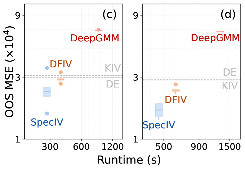
Figure 2: MSE and Runtime on dSprites Dataset with (a) Low-Dimensional Instruments (32) and (b) High-Dimensional Instruments (64), and Demand Design dataset with (c) 5,000 and (d) 10,000 training samples. Methods employing pre-specified features, i.e., DE and KIV, are represented as dashed baselines.

Figure 2a and 2b depict the performance and the execution time of various methods on the dSprites dataset. The optimal performance corresponds to proximity to the bottom-left corner, indicating low MSE and reduced runtime. SpecIV outperforms all other approaches in terms of MSE in both low- and high-dimensional contexts while maintaining a competitive runtime. Methods with fixed features, such as KIV and DE, yield high MSE. The cause might be their reliance on predetermined feature representations, which restricts adaptability. In low-dimensional scenarios, DeepGMM and DFIV manage to keep errors within a reasonable range, but DeepGMM’s performance declines sharply with increased feature dimensions, while SpecIV maintains good estimation accuracy. Furthermore, both DeepGMM and DFIV exhibit increased variance in the high-dimensional setting, possibly due to their ineffective representation learning for high-dimensional features. In summary, SpecIV demonstrates superior and consistent performance over the baseline methods in both settings for instrumental variable tasks.

Instrument Variable Regression with Observable Confounder.

In the Demand Design dataset, we employ two settings for the observable confounders. For SpecIV and DFIV, we set the ticket price $P$ as the treatment and the fuel price $C$ as the instrument, accompanied by the observables $(T,S)$. Each of these three components is presented using distinct neural networks. For other methods that don’t model observables separately, we integrate the observables directly with the treatment and instrument. This means $(P,T,S)$ is used as the treatment and $(C,T,S)$ as the instrument. Figure 2c and Figure 2d represent the performance of these approaches given different amounts of training samples. In both scenarios, SpecIV consistently delivers the lowest error also achieving the best runtime. DeepGMM performs the least efficiently, with the highest error rates and runtimes. This may result from incorporating observables into both treatment and instrument. This overlooks the fact that we only need to consider the conditional expectation of $X$ given $(Z,O)$, thus making the problem suboptimal. KIV and DE, limited by their fixed feature representations, do not benefit from an increase in training sample size and remain less expressive. Overall, the SpecIV method outperforms other approaches in learning structured functions with the presence of observable confounders.

Proxy Causal Learning.

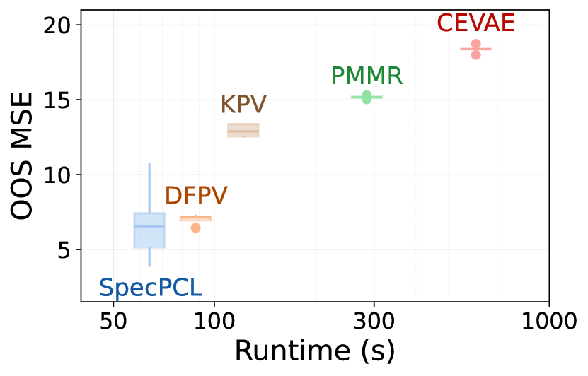
Figure 3: MSE and Runtime of structural function estimation on the dSprites dataset with 5,000 training samples.

Experimental results are shown in Figure 3. SpecPCL outperforms existing methods with superior estimation accuracy and computational efficiency, which demonstrates its strong capability in capturing complex structural functions. DFPV offers a reasonable balance between error and runtime but falls short of SpecIV’s performance. KPV appears to yield a slightly lower error, possibly because KPV harnesses a greater number of parameters to express its solution. CEVAE, despite its flexibility through neural networks, underperforms all other methods. The reason could be that CEVAE does not leverage the relation between the proxies and the structural function.

Unlabeled Data Augmentation.

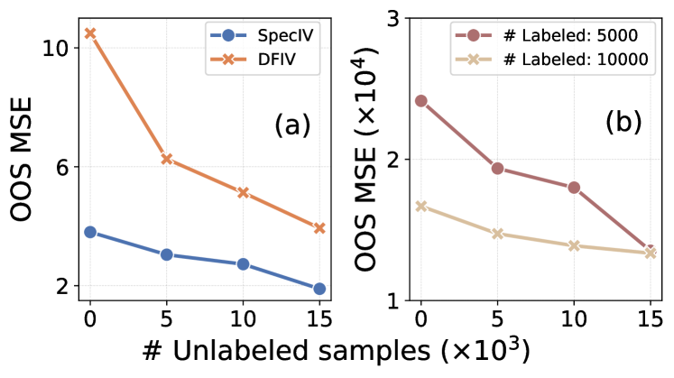
Figure 4: MSE comparison of (a) SpecIV and DFIV on dSprites dataset with 5,000 labeled training samples and (b) SpecIV on Demand Design Dataset with 5,000 and 10,000 labeled samples, respectively. Each method is trained with the specified amount of labeled data and an additional set of unlabeled samples.

In practical scenarios, it’s often easier to collect a large amount of unlabeled data than labeled data. For instance, in the Demand Design task, the true ticket demand, which is the ground-truth label, is more challenging to acquire than other readily available information like ticket price and year time. Therefore, it’s crucial to explore how much an IV method can improve by using extra unlabeled data during its training process. Note that for SpecIV with observable confounders, the unlabeled samples are used to optimize the decomposition in (12) while the original labeled data are employed for both (12) and (13). Figure 4 shows that as the number of unlabeled training samples increases (up to 3x labeled data), the MSE for both methods decreases. This trend confirms that adding unlabeled data contributes positively to the model’s performance. Notably, Figure 4a shows that SpecIV consistently achieves a lower error rate compared to DFIV. Figure 4b illustrates that incorporating additional unlabeled data can effectively compensate for the lack of labeled data and enhance model performance. This demonstrates a promising characteristic for practical applications where unlabeled data is more accessible.

6 Conclusion

We have introduced a novel spectral representation learning framework for causal estimation in the presence of hidden confounders. Our approach leverages a low-rank assumption on conditional densities to characterize function classes within a saddle-point optimization problem. This allows us to develop efficient algorithms for IV regression, both with and without observed confounders, as well as for proximal causal learning (PCL). We have demonstrated that our method outperforms existing approaches through extensive experimental validation. While we benefit from existing theoretical guarantees for IV (e.g. Bennett et al., 2023c; Wang et al., 2022), the generalization of these guarantees to IV with observed confounders and to PCL remains a challenging topic for future work. Another interesting question is to formalise the relative performance of two-stage methods vs conditional moment methods.

Appendix A Limitations and Broader Impacts

A.1 Limitations

In this paper, we introduced a novel spectral representation learning framework for causal estimation in the presence of hidden confounders. We demonstrated the superior performance of our method over existing approaches, showing reduced computational burden and increased accuracy. While our algorithm benefits from established theoretical guarantees for instrumental variables (IV) (e.g., Bennett et al., 2023c, Wang et al., 2022), our advantages for IV with observed confounders and principal component learning (PCL) are primarily justified empirical. Future work will extend existing theoretical proofs to these settings.

A.2 Broader Impacts

Potential Positive Societal Impacts. Accurately estimating causal effects has significant potential to benefit society across multiple disciplines. For example, in epidemiology, understanding causal relationships can enhance public health strategies, contributing to better disease prevention and control. This paper addresses the problem of estimating causal effects with hidden confounders. The proposed method can be effectively applied to various domains with different settings. This leads to more informed decision-making and improved outcomes in various fields.

Potential Negative Societal Impacts. While the proposed method for estimating causal effects offers multiple benefits, there are potential negative societal impacts to consider. Misapplication of the method without thorough validation could lead to incorrect conclusions and potentially harmful decisions, particularly in sensitive areas like healthcare or public policy.

Appendix B Complete Algorithms

To make our whole procedure clear, we provide the complete algorithm framework for causal estimation with spectral representation., with modifications for corresponding problems.

Algorithm 1 Spectral Representation Learning for Instrument Variable Regression

0:  Function class $\mathcal{F}$ of the representation.

  Estimate $\phi(x)$ and $\psi(z)$ with $\{x_{i},z_{i}\}$ using Equation (4.1) or Equation (16) and obtained the estimated representation $\widehat{\phi}(x)$ and $\widehat{\psi}(z)$.

  Solve the min-max problem Equation (18) and obtain the $v$ and $w$.

  $f(x)=v^{\top}\widehat{\phi}(x)$.

Algorithm 2 Spectral Representation Learning for Instrument Variable Regression with Observable Confounding

0:  Function class $\mathcal{F}_{xzo}$, $\mathcal{F}_{yzo}$.

  Estimate $\psi(z),\phi(x),V(o)$ with $\{x_{i},z_{i},o_{i}\}$ from $P(x|z,o)$ and obtained the estimated representation $\widehat{\phi}(x)$, $\widehat{V}(o)$ and $\widehat{\psi}(z)$.

  Estimate $Q(o)$, $\nu(y)$ with $P(y|z,o)$ and learned $\widehat{\psi}(z)$, $\widehat{V}(o)$ and obtain estimated $\widehat{Q}(o)$, $\widehat{\nu}(y)$.

  Solve the min-max optimization Equation (19) and obtain the $G$ and $w$.

  $f(x,o)=\left\langle G,\widehat{V}(o)^{\top}\otimes\widehat{\phi}(x)^{\top}\right\rangle$ and $u(z,o)=w^{\top}\widehat{Q}(o)^{\top}\widehat{V}(o)\widehat{\psi}(z)$.

Appendix C Identifiability

We reveal the effect of the choice of regularizer in terms of identifibility with overcomplete spectral representation in population version. We mainly focus on the IV problem in our discussion, and similar conclusion also holds for IV-OC and PCL.

Assumption 6 (Overcompleted representation).

With larger dimension $d^{\prime}\geqslant d$ for spectral representation in primal (10) and dual space (11), we obtain $\mathcal{F}^{\prime}$ and $\mathcal{U}^{\prime}$ correspondingly, with $\mathcal{F}\subseteq\mathcal{F}^{\prime}$ and $\mathcal{U}\subseteq\mathcal{U}^{\prime}$.

Proposition 5 (Least norm solution).

Under Assumption 1 and Assumption 6, with appropriate $\lambda$ in (5), the estimator provides unique solution $f$ with least $\Omega\left(f\right)$.

This can be verified by reformulating the estimator (5) into a constraint optimization, i.e.,

$$~{}\min_{f\in\mathcal{F},\varepsilon}\,\,\lambda\Omega\left(f\right)+\mathbb{E}\left[\varepsilon(s)^{2}\right]\quad\mathop{\mathrm{s.t.}},\,\mathbb{E}\left[y-f\left(x,s\right)\!\mid\!s\right]=\varepsilon\left(s\right),\quad\mathbb{P}\left(s\right)-\text{a.e.}.$$ (20)

Based on the Assumption 1 and Assumption 6, there exists one $\tilde{f}$ achieving

$$\mathbb{E}\left[y-\tilde{f}\left(x,s\right)\!\mid\!s\right]=0,\quad\mathbb{P}\left(s\right)-\text{a.e.}.$$

with the corresponding $\tilde{\varepsilon(s)}=0$. By setting an appropriate $\lambda$, the optimal solution of (20), i.e., , our estimator (5), will be $\tilde{f}$, which is the least norm solution.

Remark:

The choice of $\Omega\left(f\right)$ reveals an interesting but largely ignored topic on the definition of idenfiability with representation learning. Specifically, in the classic IV setting [Liao et al., 2020, Bennett et al., 2023b], the function space with norm is given and assumed to be realizable, i.e., the function space contains the groundtruth target function. Therefore, the least norm identifiability [Bennett et al., 2023b, Li et al., 2024] is naturally based on the norm of the given function space. However, we are aiming for identifying both the function space and the target function by exploiting the representation learning, where the function space is learned, therefore, no norm is predefined.

Our representation characterization in Section 3 clearly provides measure-dependent norms. Specifically, the representation is intimately coupled with the inner product w.r.t. a base measure, which naturally induces norms. We take IV as an example, we exploit the inner product w.r.t. $P\left(x\right)$, which induces the norm $\left\|\cdot\right\|_{L_{2}\left(P_{x}\right)}$. Meanwhile, since $f=v^{\top}\phi\left(x\right)\in\mathcal{R}\left(\phi\right)$ as shown in Proposition 2, we can also simply set $\left\|f\right\|_{\mathcal{R}(\phi)}^{2}:=v^{\top}v$. We emphasize our characterization reveals the importance of base measure in representation learning stage and least norm estimation stage. For different $P(x)$ and the induced space $L_{2}(P_{x})$, our method can have a different set of the learned representation of $\phi(x)$, and potentially leads to different norm definitions, and thus, different least norm solution when the Fredholm equation (1) is unidentifiable.

Intuitively, the inner product with the measure plays as an essential prior implies the region we should focus in causal estimation.

Appendix D Proofs of Section 3

We present the omitted proofs of Section 3.

D.1 Proof of Proposition 1

The proof is in the main text.

D.2 Proof of Proposition 2

Notice that the subspace $\mathcal{R}\left(\Phi\right)$ of $L_{2}\left(P_{x}\right)$ is closed by continuity of the inner product in $\mathbb{R}^{d}$. Therefore, it is in direct sum with its orthogonal, i.e., $L_{2}\left(P_{x}\right)=\mathcal{R}\left(\Phi\right)\oplus\mathcal{R}\left(\Phi\right)^{\perp}$ (Theorem 3.3.4. in Kreyszig, 1991). Following this observation, we write $f\in L_{2}\left(P_{x}\right)$ as $f=\left\langle\mathbf{u}_{f},\varphi\left(\cdot\right)\right\rangle+h^{\perp}$, with $\mathbf{u}_{f}\in\mathbb{R}^{d}$, $h^{\perp}\in\mathcal{R}\left(\Phi\right)^{\perp}$, and we have

$$\mathcal{T}f\left(z\right) =\int_{\mathcal{X}}\left(\left\langle\mathbf{u}_{f},\varphi\left(x\right)\right\rangle+h^{\perp}\left(x\right)\right)\left\langle\phi\left(x\right),\psi\left(z\right)\right\rangle\mathop{}\!\mathrm{d}P_{x}$$ (Assumption 2)

$$=\left\langle\mathbf{u}_{f},\left(\int_{\mathcal{X}}\varphi\left(x\right)\varphi\left(x\right)^{\mathsf{\scriptscriptstyle T}}\mathop{}\!\mathrm{d}P_{x}\right)\psi\left(z\right)\right\rangle_{\mathbb{R}^{d}}+\left\langle h^{\perp},\Phi\psi\left(z\right)\right\rangle_{L_{2}\left(P_{x}\right)}$$

$$=\left\langle\mathbf{u}_{f},\left(\int_{\mathcal{X}}\varphi\left(x\right)\varphi\left(x\right)^{\mathsf{\scriptscriptstyle T}}\mu\left(dx\right)\right)\psi\left(z\right)\right\rangle_{\mathbb{R}^{d}} \left(h^{\perp}\in\mathcal{R}\left(\Phi\right)^{\perp}\right).$$

Notice we also have

$$\lVert f\rVert_{L_{2}\left(P_{x}\right)}^{2} =\mathbb{E}\left[f\left(x\right)^{2}\right]$$

$$=\mathbb{E}\left[\left\langle\mathbf{u}_{f},\phi\left(x\right)\right\rangle^{2}\right]+\mathbb{E}\left[h^{\perp}\left(x\right)^{2}\right] \left(h^{\perp}\perp\left\langle\mathbf{u}_{f},\varphi\left(\cdot\right)\right\rangle\right)$$

$$=\left\langle\mathbf{u}_{f},\mathbb{E}\left[\varphi\left(x\right)\varphi\left(x\right)^{\mathsf{\scriptscriptstyle T}}\right]\mathbf{u}_{f}\right\rangle+\mathbb{E}\left[h^{\perp}\left(x\right)^{2}\right].$$

This shows $h^{\perp}$ influences the objective function only through $\mathbb{E}\left[h^{\perp}\left(x\right)^{2}\right]$. Since we are minimizing for $f$, we can set $h^{\perp}=0$ and only consider $f\in\mathcal{R}\left(\Phi\right)$.

Furthermore, Assumption 1 states there exists a solution to Problem 2. Using the same decomposition, this provides a solution to Problem 2 in $\mathcal{R}\left(\Phi\right)$. This concludes the proof.

D.3 Proof of Proposition 3

Proof.

By plugging Equation (13) into the RHS of Equation (3), we obtain

$$\left\langle\psi(z),V(o)^{\top}\left[\int\phi(x)\phi\left(x\right)^{\top}dP_{x}\right]v(o)\right\rangle=\left\langle\psi\left(z\right),W(o)^{\top}\int y\nu(y)dP_{y}\right\rangle,$$

Using the fact that $\psi$ spans every direction,

$$V\left(o\right)^{\top}\underbrace{\left[\int\phi\left(x\right)\phi\left(x\right)^{\top}\mathop{}\!\mathrm{d}P_{x}\right]}_{:=A}v\left(o\right)=W\left(o\right)^{\top}\underbrace{\int y\nu\left(y\right)\mathop{}\!\mathrm{d}P_{y}}_{:=\alpha}.$$

We can now characterize the space of $v(o)$. Specifically, we have

$$v\left(o\right)=A^{+}\left(V\left(o\right)^{\top}\right)^{+}W\left(o\right)^{\top}\alpha.$$ (21)

Finding the space of $v(o)$ requires taking several (pseudo-)inverses, which is computationally expensive. We can instead use an alternative parametrization in $Q\left(o\right):=\left(V(o)^{\top}\right)^{+}W(o)^{\top}$, which gives $W\left(o\right)=Q\left(o\right)^{\top}V\left(o\right)$ in Equation (13). This leads to the desired parametrization. ∎

D.4 Proof of Proposition 4

The argument from Proposition 1 also applies here.

Appendix E Experiment Details

Setup.

For the IV tasks, each method is assessed using a test set comprising 2,000 samples, while for the PCL task, the evaluation is based on a test set of 500 samples. The test samples are randomly generated using the same data generation setting as the training set. All experiments are conducted on a system equipped with an Intel(R) Xeon(R) Silver 4114 CPU @ 2.20GHz and a Quadro RTX 8000 GPU. Note that for IV with observable confounders, we simplify the implementation by omitting the decomposition of $P(x|z)$. This helps reduce the number of parameters that need to be optimized.

Hyperparameters.

For the IV regression experiments, we employ the same hyper-parameter setting for DFIV, KIV, and DeepGMM used in Xu et al. [2020]. For DE, we use the same Gaussian kernel with the bandwidth determined by the median trick Singh et al. [2019]. The network structures for SpecIV on different datasets are provided in Table 3 and 4.

Dataset Dimensions.

The feature dimensions for these configurations are presented in Table 1.

Table 1: Dimensions of treatment, instrument, and observable confounder Variables in two datasets with varying settings. In the dSprites dataset, the ’low’ and ’high’ dimensions pertain to the instrument feature dimension. In the Demand Design dataset, ’SC’ represents separated observable confounders. SpecIV and DFIV are assessed with separate representations for the observables. The remaining baseline methods are evaluated without separate observables, i.e., , via incorporating these confounders into both treatment and instrumental variables.

Dataset	dSprites		Demand Design
	Low-dim	High-dim	With SC	No SC
Treatment	4,096	4,096	784	1,569
Instrument	3	2,352	1	786
Observable	-	-	785	-

Table 2: Network Structure of the feature extractor for Demand Design dataset. Each 2D convolutional layer (Conv2d) is depicted with (input dimension, output dimension, kernel size, stride, padding).

ImageFeature
Layer	Configuration
1	Input: 784
2	Conv2d(1, 16, 5, 1, 2), ReLU, MaxPool2d
3	Conv2d(16, 32, 5, 1, 2), ReLU, MaxPool2d
4	FC$(1568,1024)$

Table 3: Network Structure of SpecIV for IV on the dSprites dataset. The tuple for each component represents the input/output dimensions within a particular component. FC refers to the fully-connected layers. BN represents batch normalization.

Treatment Feature Net (32)
Layer	Configuration
1	Input: 4096
2	FC$(4096,1024)$, ReLU, BN
3	FC$(1024,512)$, ReLU, BN
4	FC$(512,128)$, ReLU, BN
5	FC$(128,32)$, tanh

Instrument Feature Net (32)
Layer	Configuration
1	Input: 3
2	FC$(3,256)$, ReLU, BN
3	FC$(256,128)$, ReLU, BN
4	FC$(128,128)$, ReLU, BN
5	FC$(128,32)$, ReLU

Treatment Feature Net (64) Layer Configuration 1 Input: 4096 2 FC$(4096,1024)$, ReLU, BN 3 FC$(1024,256)$, ReLU, BN 4 FC$(256,64)$, tanh Instrument Feature Net (64) Layer Configuration 1 Input: 2352 2 FC$(2352,1024)$, ReLU, BN 3 FC$(1024,256)$, ReLU, BN 4 FC$(256,64)$, ReLU

Table 4: Network Structure of SpecIV for IV on the Demand Design dataset. The tuple for each component represents the input/output dimensions within a particular component. FC refers to the fully-connected layers. BN represents batch normalization. ImageFeature indicates the feature extractor detailed in Table 2.

Treatment Feature Net (32)
Layer	Configuration
1	Input: 784 (P)
2	ImageFeature(P)
3	FC$(1024,512)$, ReLU, BN
4	FC$(512,256)$, ReLU, BN
5	FC$(256,32)$, tanh

Observable Feature Net (32)
Layer	Configuration
1	Input: 785 (T, S)
2	ImageFeature(S), T
3	FC$(1025,512)$, ReLU, BN
4	FC$(512,256)$, ReLU,BN
5	FC$(256,32)$, tanh

Instrument Feature Net (32) Layer Configuration 1 Input: 1 2 FC$(1,16)$, ReLU, BN 3 FC$(16,4)$, ReLU Outcome Feature Net (32) Layer Configuration 1 Input: 1 2 FC$(1,16)$, ReLU, BN 3 FC$(16,4)$, ReLU

Table 5: Network Structure of SpecPCL for PCL on the dSprites dataset. The tuple for each component represents the input/output dimensions within a particular component. FC refers to the fully-connected layers. BN represents batch normalization.

Treatment Feature Net
Layer	Configuration
1	Input: 4096
2	FC$(4096,1024)$, ReLU, BN
3	FC$(1024,512)$, ReLU, BN
4	FC$(512,32)$, tanh

Observable Feature Net
Layer	Configuration
1	Input: 4096
2	FC$(4096,1024)$, ReLU, BN
3	FC$(1024,256)$, ReLU,BN
4	FC$(256,32)$, tanh

Instrument Feature Net
Layer	Configuration
1	Input: 3
2	FC$(3,16)$, ReLU, BN
3	FC$(16,2)$, ReLU

Outcome Feature Net
Layer	Configuration
1	Input: 1
2	FC$(1,16)$, ReLU, BN
3	FC$(16,2)$, ReLU

Appendix F Dimension Mapping

We utilize the mapping function in Bennett et al. [2019] to build the high-dimensional scenarios. Given a low-dimensional input $X_{\text{low}}\in\mathbb{R}$, we generate a corresponding high-dimensional variable $X_{\text{high}}\in\mathbb{R}^{784}$ via:

$$X_{\text{high}}=\text{RandomImage}(\pi(X_{\text{low}}))$$ (22)

where $\pi(x)=\text{round}(\min(\max(1.5x+5,0),9))$ transforms the input to an integer within the range 0 to 9; $\text{RandomImage}(d)$ selects a random MNIST image corresponding to the input digit $d$.

Appendix G Data Generation for dSprites

G.1 IV Task

We generate data using the following relationships:

$$f(X) =\frac{\|AX\|^{2}_{2}-5000}{1000},$$

$$Y =f(X)+32(\texttt{posX}-0.5)+\varepsilon,\,\,\varepsilon\sim\mathcal{N}(0,0.5).$$

where each entry of $A\in\mathbb{R}^{10\times 4096}$ is drawn from $\text{Uniform}(0,1)$. We generate $A$ once initially and maintain it fixed throughout the experiment.

The relationship above allows us to generate the treatment $X\in\mathbb{R}^{4096}$ and the instrument $Z\in\mathbb{R}^{3}$, denoted as the low-dimensional scenario. By applying equation (22) to each element of $Z$, we can transform these into a high-dimensional scenario, i.e., , $Z_{\text{high}}\in\mathbb{R}^{2352}$.

G.2 PCL Task

For the PCL setting, we employ the same definition of $f(\cdot)$ and obtain $Y$ through:

$$Y =\frac{1}{12}(\texttt{posX}-0.5)f(X)+\varepsilon,\,\,\varepsilon\sim\mathcal{N}(0,0.5).$$

We conduct the structural function estimation experiment on dSprites with treatment in $\mathbb{R}^{4096}$ and instrument in $\mathbb{R}^{3}$. Following Xu et al. [2021], we fix the shape as heart and use (scale, rotation, posX) as the treatment-inducing proxy. We then sample another image from the dSprites dataset with the same posY as the output-inducing proxy, i.e., , $\text{Image({scale}=0.8, {rotation}=0, {posX}=0.5, {posY})}+{\eta}$, with $\eta\sim\mathcal{N}(0,0.1I)$.

Appendix H Data Generation for Demand Design

Following Singh et al. [2019], we generate data samples using the following relationships:

$$Y =f(P,T,S)+\varepsilon$$

$$f(P,T,S) =100+(10+p)Sh(T)-2P$$

$$h(t) =2\left(\dfrac{(t-5)^{4}}{600}+\exp(-4(t-5)^{2})+\dfrac{t}{10}-2\right)$$

with

$$S \sim\text{Uniform}\{1,\dots,7\}$$

$$T \sim\text{Uniform}[0,10]$$

$$C \sim\mathcal{N}(0,1)$$

$$V \sim\mathcal{N}(0,1)$$

$$\varepsilon \sim\mathcal{N}(\rho V,1-\rho^{2})$$

$$P =25+(C+3)h(T)+V$$

The mapping function (22) is then used to generate high-dimensional versions of the variables $P$ and $S$. This results in $P,S\in\mathbb{R}^{784}$ and $T,C\in\mathbb{R}$.

References

- Antos et al. [2008] András Antos, Csaba Szepesvári, and Rémi Munos. Learning near-optimal policies with bellman-residual minimization based fitted policy iteration and a single sample path. Machine Learning, 71:89–129, 2008.
- Bennett et al. [2019] Andrew Bennett, Nathan Kallus, and Tobias Schnabel. Deep generalized method of moments for instrumental variable analysis. Advances in neural information processing systems, 32, 2019.
- Bennett et al. [2023a] Andrew Bennett, Nathan Kallus, Xiaojie Mao, Whitney Newey, Vasilis Syrgkanis, and Masatoshi Uehara. Inference on strongly identified functionals of weakly identified functions. In The Thirty Sixth Annual Conference on Learning Theory, pages 2265–2265. PMLR, 2023a.
- Bennett et al. [2023b] Andrew Bennett, Nathan Kallus, Xiaojie Mao, Whitney Newey, Vasilis Syrgkanis, and Masatoshi Uehara. Minimax instrumental variable regression and convergence guarantees without identification or closedness. In The Thirty Sixth Annual Conference on Learning Theory, pages 2291–2318. PMLR, 2023b.
- Bennett et al. [2023c] Andrew Bennett, Nathan Kallus, Xiaojie Mao, Whitney Newey, Vasilis Syrgkanis, and Masatoshi Uehara. Source condition double robust inference on functionals of inverse problems. arXiv preprint arXiv:2307.13793, 2023c.
- Bradtke and Barto [1996] Steven J Bradtke and Andrew G Barto. Linear least-squares algorithms for temporal difference learning. Machine learning, 22(1):33–57, 1996.
- Chen and Christensen [2018] Xiaohong Chen and Timothy M. Christensen. Optimal sup-norm rates and uniform inference on nonlinear functionals of nonparametric iv regression: Nonlinear functionals of nonparametric iv. Quantitative Economics, 9(1):39–84, March 2018. ISSN 1759-7323. doi: 10.3982/qe722. URL http://dx.doi.org/10.3982/QE722.
- Dai et al. [2017] Bo Dai, Niao He, Yunpeng Pan, Byron Boots, and Le Song. Learning from conditional distributions via dual embeddings. In Artificial Intelligence and Statistics, pages 1458–1467. PMLR, 2017.
- Darolles et al. [2011] Serge Darolles, Yanqin Fan, Jean-Pierre Florens, and Eric Renault. Nonparametric instrumental regression. Econometrica, 79(5):1541–1565, 2011.
- Deaner [2018] Ben Deaner. Proxy controls and panel data. arXiv preprint arXiv:1810.00283, 2018.
- Dikkala et al. [2020] Nishanth Dikkala, Greg Lewis, Lester Mackey, and Vasilis Syrgkanis. Minimax estimation of conditional moment models. Advances in Neural Information Processing Systems, 33:12248–12262, 2020.
- Engl et al. [1996] Heinz Werner Engl, Martin Hanke, and Andreas Neubauer. Regularization of inverse problems, volume 375. Springer Science & Business Media, 1996.
- Grunewalder et al. [2012] S. Grunewalder, G. Lever, L. Baldassarre, S. Patterson, A. Gretton, and M. Pontil. Conditional mean embeddings as regressors. In International Conference on Machine Learning, 2012.
- Hartford et al. [2017] Jason Hartford, Greg Lewis, Kevin Leyton-Brown, and Matt Taddy. Deep iv: A flexible approach for counterfactual prediction. In International Conference on Machine Learning, pages 1414–1423. PMLR, 2017.
- Horowitz [2011] Joel L Horowitz. Applied nonparametric instrumental variables estimation. Econometrica, 79(2):347–394, 2011.
- Jin et al. [2020] Chi Jin, Zhuoran Yang, Zhaoran Wang, and Michael I Jordan. Provably efficient reinforcement learning with linear function approximation. In Conference on Learning Theory, pages 2137–2143. PMLR, 2020.
- Kompa et al. [2022] Benjamin Kompa, David Bellamy, Tom Kolokotrones, Andrew Beam, et al. Deep learning methods for proximal inference via maximum moment restriction. Advances in Neural Information Processing Systems, 35:11189–11201, 2022.
- Kreyszig [1991] Erwin Kreyszig. Introductory functional analysis with applications, volume 17. John Wiley & Sons, 1991.
- Kuroki and Pearl [2014] Manabu Kuroki and Judea Pearl. Measurement bias and effect restoration in causal inference. Biometrika, 101(2):423–437, 2014.
- Li et al. [2022] Zhu Li, Dimitri Meunier, Mattes Mollenhauer, and Arthur Gretton. Optimal rates for regularized conditional mean embedding learning. In Advances in Neural Information Processing Systems, 2022.
- Li et al. [2024] Zihao Li, Hui Lan, Vasilis Syrgkanis, Mengdi Wang, and Masatoshi Uehara. Regularized deepiv with model selection. arXiv preprint arXiv:2403.04236, 2024.
- Liao et al. [2020] Luofeng Liao, You-Lin Chen, Zhuoran Yang, Bo Dai, Mladen Kolar, and Zhaoran Wang. Provably efficient neural estimation of structural equation models: An adversarial approach. Advances in Neural Information Processing Systems, 33:8947–8958, 2020.
- Louizos et al. [2017] Christos Louizos, Uri Shalit, Joris M Mooij, David Sontag, Richard Zemel, and Max Welling. Causal effect inference with deep latent-variable models. Advances in neural information processing systems, 30, 2017.
- Mastouri et al. [2021] Afsaneh Mastouri, Yuchen Zhu, Limor Gultchin, Anna Korba, Ricardo Silva, Matt Kusner, Arthur Gretton, and Krikamol Muandet. Proximal causal learning with kernels: Two-stage estimation and moment restriction. In International conference on machine learning, pages 7512–7523. PMLR, 2021.
- Mastouri et al. [2023] Afsaneh Mastouri, Yuchen Zhu, Limor Gultchin, Anna Korba, Ricardo Silva, Matt J. Kusner, Arthur Gretton, and Krikamol Muandet. Proximal causal learning with kernels: Two-stage estimation and moment restriction, 2023.
- Matthey et al. [2017] Loic Matthey, Irina Higgins, Demis Hassabis, and Alexander Lerchner. dsprites: Disentanglement testing sprites dataset. https://github.com/deepmind/dsprites-dataset/, 2017.
- Miao et al. [2018] Wang Miao, Zhi Geng, and Eric J Tchetgen Tchetgen. Identifying causal effects with proxy variables of an unmeasured confounder. Biometrika, 105(4):987–993, 2018.
- Muandet et al. [2020] Krikamol Muandet, Arash Mehrjou, Si Kai Lee, and Anant Raj. Dual instrumental variable regression. In Advances in Neural Information Processing Systems, volume 33, pages 2710–2721. Curran Associates, Inc., 2020.
- Newey and Powell [2003] Whitney K Newey and James L Powell. Instrumental variable estimation of nonparametric models. Econometrica, 71(5):1565–1578, 2003.
- Qiu et al. [2022] Shuang Qiu, Lingxiao Wang, Chenjia Bai, Zhuoran Yang, and Zhaoran Wang. Contrastive ucb: Provably efficient contrastive self-supervised learning in online reinforcement learning. In International Conference on Machine Learning, pages 18168–18210. PMLR, 2022.
- Ren et al. [2022a] Tongzheng Ren, Chenjun Xiao, Tianjun Zhang, Na Li, Zhaoran Wang, Sujay Sanghavi, Dale Schuurmans, and Bo Dai. Latent variable representation for reinforcement learning. arXiv preprint arXiv:2212.08765, 2022a.
- Ren et al. [2022b] Tongzheng Ren, Tianjun Zhang, Lisa Lee, Joseph E Gonzalez, Dale Schuurmans, and Bo Dai. Spectral decomposition representation for reinforcement learning. arXiv preprint arXiv:2208.09515, 2022b.
- Singh et al. [2019] Rahul Singh, Maneesh Sahani, and Arthur Gretton. Kernel instrumental variable regression. Advances in Neural Information Processing Systems, 32, 2019.
- Song et al. [2009] Le Song, Jonathan Huang, Alexander Smola, and Kenji Fukumizu. Hilbert space embeddings of conditional distributions with applications to dynamical systems. In International Conference on Machine Learning, pages 961 – 968, 2009.
- Stock and Watson [2007] James Stock and Mark Watson. Introduction to Econometrics 2nd edition. Prentiss Hall, 2007.
- Stock and Trebbi [2003] James H Stock and Francesco Trebbi. Retrospectives: Who invented instrumental variable regression? Journal of Economic Perspectives, 17(3):177–194, 2003.
- Sutton and Barto [2018] Richard S Sutton and Andrew G Barto. Reinforcement learning: An introduction. MIT press, 2018.
- Wang et al. [2022] Ziyu Wang, Yucen Luo, Yueru Li, Jun Zhu, and Bernhard Schölkopf. Spectral representation learning for conditional moment models. arXiv preprint arXiv:2210.16525, 2022.
- Wright [1928] Philip Green Wright. The tariff on animal and vegetable oils. Number 26. Macmillan, 1928.
- Xu et al. [2020] Liyuan Xu, Yutian Chen, Siddarth Srinivasan, Nando de Freitas, Arnaud Doucet, and Arthur Gretton. Learning deep features in instrumental variable regression. arXiv preprint arXiv:2010.07154, 2020.
- Xu et al. [2021] Liyuan Xu, Heishiro Kanagawa, and Arthur Gretton. Deep proxy causal learning and its application to confounded bandit policy evaluation. Advances in Neural Information Processing Systems, 34:26264–26275, 2021.
- Yang and Wang [2020] Lin Yang and Mengdi Wang. Reinforcement learning in feature space: Matrix bandit, kernels, and regret bound. In International Conference on Machine Learning, pages 10746–10756. PMLR, 2020.
- Zhang et al. [2023] Rui Zhang, Masaaki Imaizumi, Bernhard Schölkopf, and Krikamol Muandet. Instrumental variable regression via kernel maximum moment loss. Journal of Causal Inference, 11(1), 2023.
- Zhang et al. [2022] Tianjun Zhang, Tongzheng Ren, Mengjiao Yang, Joseph Gonzalez, Dale Schuurmans, and Bo Dai. Making linear mdps practical via contrastive representation learning. In International Conference on Machine Learning, pages 26447–26466. PMLR, 2022.