A generalized geometric mechanics theory for multi-curve-fold origami: vertex constrained universal configurations
Abstract
Folding paper along curves leads to spatial structures that have curved surfaces meeting at spatial creases, defined as curve-fold origami. In this work, we provide an Eulerian framework focusing on the mechanics of arbitrary curve-fold origami, especially for multi-curve-fold origami with vertices. We start with single-curve-fold origami that has wide panels. Wide panel leads to different domains of mechanical responses induced by various generator distributions of the curved surface. The theories are then extended to multi-curve-fold origami, involving additional geometric correlations between creases. As an illustrative example, the deformation and equilibrium configuration of origami with annular creases are studied both theoretically and numerically. Afterward, single-vertex curved origami theory is studied as a special type of multi-curve-fold origami. We find that the extra periodicity at the vertex strongly constrains the configuration space, leading to a region near the vertex that has a striking universal equilibrium configuration regardless of the mechanical properties. Both theories and numerics confirm the existence of the universality in the near-field region. In addition, the far-field deformation is obtained via energy minimization and validated by finite element analysis. Our generalized multi-curve-fold origami theory, including the vertex-contained universality, is anticipated to provide a new understanding and framework for the shape programming of the curved fold origami system.
keywords:
Origami , Curved folds , Isometric deformation , Geometric mechanics , Nonlinear elasticity[inst1]organization=State Key Laboratory for Turbulence and Complex Systems, Department of Mechanics and Engineering Science, BIC-ESAT, College of Engineering, Peking University,city=Beijing, postcode=100087, country=China
[inst2]organization=HEDPS, CAPT and IFSA, Collaborative Innovation Center of MoE, Peking University,city=Beijing, postcode=100087, country=China
[inst3]organization=Department of Mechanics and Engineering Science, College of Engineering, Peking University,city=Beijing, postcode=100087, country=China
1 Introduction
Origami is an ancient art form aiming to achieve complex spatial shapes by folding planar sheets. Classic origami only involves folding along straight lines, and it was not until the 1920s that students in Bauhaus realized sheets could be folded along curves, unveiling a novel branch that expands the traditional art form (Koschitz et al., 2008; Demaine et al., 2011). This new branch, defined as curved fold origami, opens new possibilities in origami design. Beyond art design, recently curved fold origami has found applications in soft robotics (Baek et al., 2020; Rus and Sung, 2018; Feng et al., 2024) metamaterials (Lee et al., 2021; Karami et al., 2024; Sun et al., 2024), architecture (Tachi and Epps, 2011; Mouthuy et al., 2012) and virtual reality technology (Zhang et al., 2023), due to its extraordinary abilities in energy storage, fast deployment and stiffness manipulation.
The scientific exploration of curved fold origami originated with the pioneering work by David Huffman (1976). In the groundwork, curved origami structures are assumed to deform isometrically, thus they are geometrically modeled as developable surfaces meeting at space curves. Harnessing the theory of curves and surfaces in differential geometry (Do Carmo, 1976), the geometrical theories of curved origami are developed in subsequent works (Duncan and Duncan, 1982; Fuchs and Tabachnikov, 1999; Kilian et al., 2008; Demaine et al., ), revealing the geometric correlations between curved folds and bent panels. The foundational results in this area are: Given the reference strips, the two developable surfaces are determined by the space crease in the deformed configurations. The theories contribute to the computational design of developable surfaces (Rabinovich et al., 2018) and curve-fold origami (Mitani, 2011; Mitani and Igarashi, 2011; Tachi, 2013; Jiang et al., 2019; Sasaki and Mitani, 2022; Mundilova et al., 2023), as well as the predicted shape of Möbius strip (Starostin and van der Heijden, 2007; Audoly and Van der Heijden, 2023).
Built upon geometric correlations, the mechanical properties of single-curved-fold origami have been investigated. The isometric deformation of curve-fold origami is determined via elastic energy (creases’ folding energy + panels’ bending energy) minimization under the constraints of developability. Mechanically, creases are modeled as elastic hinges distributed along curves and panels are modeled as unstrechable Kirchhoff plates with energy density proportional to the principle curvatures’ square. Due to the foundational results in geometric works, the bending energy of developable surfaces reduces to a -dimensional integral of the energy functional associated with the geometry of reference curves. The exact form of the bending energy is derived by Wunderlich (Wunderlich, 1962; Dias and Audoly, 2015; Todres, 2015), which degenerates to the more widely used Sadowsky (1930) functional in narrow panels (Starostin and van der Heijden, 2007; Dias et al., 2012; Dias and Audoly, 2014; Yu and Hanna, 2019). Taken together, the entire elastic energy is expressed as an integral along the crease, determined by the crease’s geometry. Minimizing the energy yields the equilibrium geometry of the deformed crease as well as the configuration of the entire origami.
In the area of geometric mechanics, the deformation of an annular sheet folding along its centerline is studied in Dias et al. (2012). The energy functional is expressed with curvature and torsion of the deformed fold. Minimizing the energy leads to an equilibrium configuration that can be described analytically with . The theoretical results capture the buckling phenomenon well. The theory is further extended to derive a nonlinear rod model for folded elastic narrow strips (Dias and Audoly, 2014). In the work, curved origami is fitted into the framework of thin rods (Moulton et al., 2013), which simplifies numerical solving and stability analyses. In other studies, panels are constrained to deform cylindrically, thus the deformation is derived by generalized Euler-Bernoulli beam theory (Lee et al., 2018). General theory for curved origami with arbitrary deformation and reference shapes is absent. Beyond single-curve-fold origami, some works study structures with multiple curved folds (Dias and Santangelo, 2012; Liu and James, 2024). The geometric design and elastic energy of some specific multi-curve-fold origami are studied, but how geometry and elasticity contribute to the deformation of multi-curve-fold structures is still poorly understood.
In this paper, we derive a generalized theory for the deformation of multi-curve-fold origami, particularly with vertices. Our theory reveals a remarkable universality in this system: the deformed configuration of a multi-curve-fold origami near the vertex is solely determined by the symmetry at the vertex and independent of the mechanical properties. To this end, we first derive a generalized theory for single-curve-fold origami, removing the narrow panel assumption in many related works. The most significant differences between narrow and wide panels are: geometrically, all generators of a developable surface start from the crease and end at the opposite edge, while in wide panels, generator distribution is more complex; mechanically, different generator distributions yield various mechanical responses. On the geometry side, we classify the generator distribution comprehensively for wide panels, and on the mechanics side, we utilize the Wunderlich theory to derive the energy density for different generator distributions precisely. Equilibrium configurations are then obtained via energy minimization.
Based on the single-curve-fold theory, we extend the theoretical framework to multi-curve-fold origami by introducing geometric correlations between creases. Such correlations result in the propagation of generators and deformations between adjacent creases, which are solved by a numerical scheme. Accordingly, the energy distribution is also derived, leading to the geometric mechanics theory of multi-curve-fold origami. Validations are made on an illustrative structure with multiple annular folds, where theoretical and finite element analysis (FEA) results fit well.
More interestingly, we find that a mechanics-independent deformed configuration emerges when the multiple creases meet at a vertex. We prove that in the system of multi-curve-fold origami with a vertex, the periodicity at the vertex yields a universal equilibrium configuration in the domain near the vertex, regardless of mechanical properties (stiffness of folds and panels) and geodesic curvatures of folds. Specifically, the deformed configuration is determined only by the folding angle at the vertex. In contrast, in the far-field domain determined by the aforementioned geometric correlations, the energy minimization yields various equilibrium configurations for different mechanical constants. Both results are validated by FEA. The theories allow us to predict the deformation of multi-curve-fold origami with vertices.
The paper is organized as follows. In Section 2, we start with the preliminaries of differential geometry for the deformation of a single strip and then develop a generalized theory for single-curve-fold origami with arbitrary reference shapes and wide panels. The theory is extended to multi-curve-fold theory by deriving the correlations between creases in Section 3. Based on the theory, multi-curve-fold origami with a vertex is theoretically studied in Section 4, which is compared with numerical results. Finally, Section 5 concludes the main points of this paper.
2 Single-curve-fold origami theory
2.1 Preliminaries: geometry of single-curve-fold origami
We start with the classic differential geometry for the shape description of curved fold origami in the deformed domain, i.e., in the Eulerian framework. In this paper, we assume the origami structure is deformed isometrically from a flat sheet. Therefore, the flanks are modeled as developable surfaces, which are generically given by
| (1) |
with the developability constraint
| (2) |
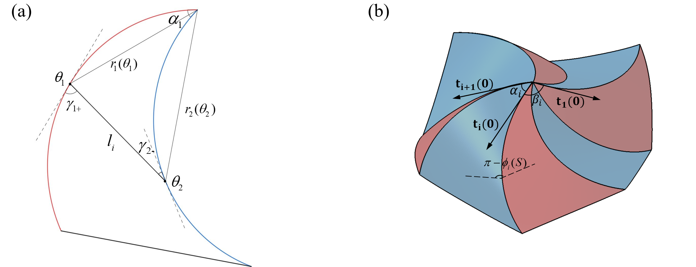
Here is a selected reference curve on the surface, and is the generator at the arclength . In curved-fold origami, it is convenient to choose the curved crease as the reference curve and the flanks on the two sides are described by Eq. (1). Solving these two equations yields strong geometric correlations between the reference curve and the developable surface, which are given explicitly via solving the kinematic equations of Frenet frames and Darboux frames (shown in Fig. 1(a)).
Frenet frame is a moving frame on a space curve that consists of the unit tangent , the unit normal , and the unit binormal . The derivatives of the vectors along the curve are
| (3) | ||||
where and are the curvature and torsion, which determine the shape of the space curve uniquely up to rigid motions by the fundamental theorem of curves (Do Carmo (1976)).
Darboux frame is a moving frame on a surface that consists of , , where , are on the tangent plane and is the unit normal of the surface. For a developable surface, we select
| (4) | ||||
to connect the different frames, and the selection makes sure that the frame will not change its direction when moving along a generator. Thus the Darboux vectors only relate to the arc length and the kinematic equations are
| (5) | ||||
where is the differential form representing the rotation of the Darboux frame. The nonzero principle curvature satisfies
| (6) | ||||
Geodesic curvature and normal curvature of the curve on surface are defined as
| (7) | ||||
The geodesic curvature is constant during isometric deformation, thus it only depends on the reference planar shape. To describe the distribution of generators we define
| (8) |
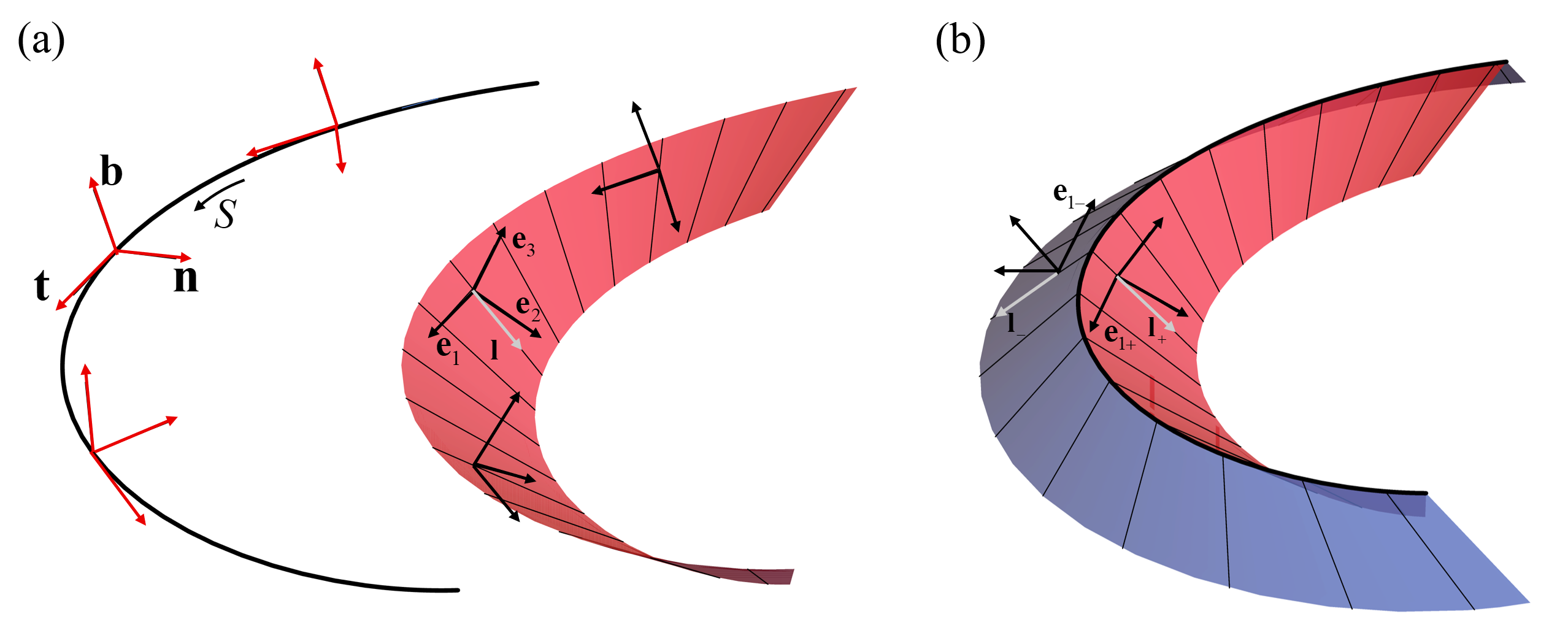
and the generator vector is selected as
| (9) |
According to Eq. (2) - (7), the derivatives are written as
| (10) | ||||
and the nonzero principle curvature is derived by
| (11) |
On the premise of developability, the generators cannot intersect with each other inside the surface, thus stays positive along any generator. The generators may intersect at boundaries of the surface, forming a conical point introducing singularity of .
Furthermore, the torsion can be expressed using Darboux frame
| (12) |
Therefore, the principle curvature distribution on the panel depends on the curvature and torsion of the curved fold, according to Eq. (7), (11) and (12). Symmetrically we derive the geometric variables in the opposite panel
| (13) | ||||
Notice that the Darboux frames of panel and panel are illustrated in Fig. 1(b), where the positive directions of are defined in opposite directions for convenience. For single-curve-fold origami with a nonzero is classified as non-developable curved origami (Duffy et al., 2021; Feng et al., 2022; Zou et al., 2024), which can be obtained by stitching together two separate curved strips. In this paper, we focus on the developable case (), meaning that the origami is folded from a single sheet of paper.
Folding angle is a key characteristic of origami involving folding energy. In curved origami, the folding angle may vary along the curve, defined as
| (14) |
which only depends on .
2.2 Domain classification for curved fold origami with wide flanks
As analyzed in the previous section, generators determine the deformation of panels. Therefore, before moving to mechanics, a discussion on domain classification based on generator distribution is needed. Previous works concerning curved origami assume that all generators starting from the crease end at the opposite edge, while in wide panels this assumption breaks. A comprehensive domain classification is analyzed in this section.
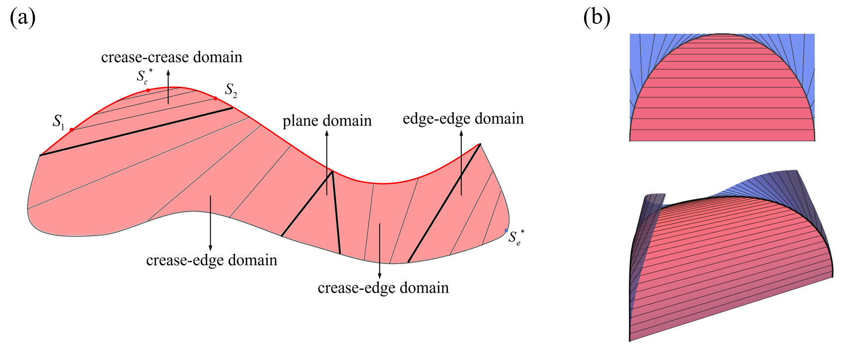
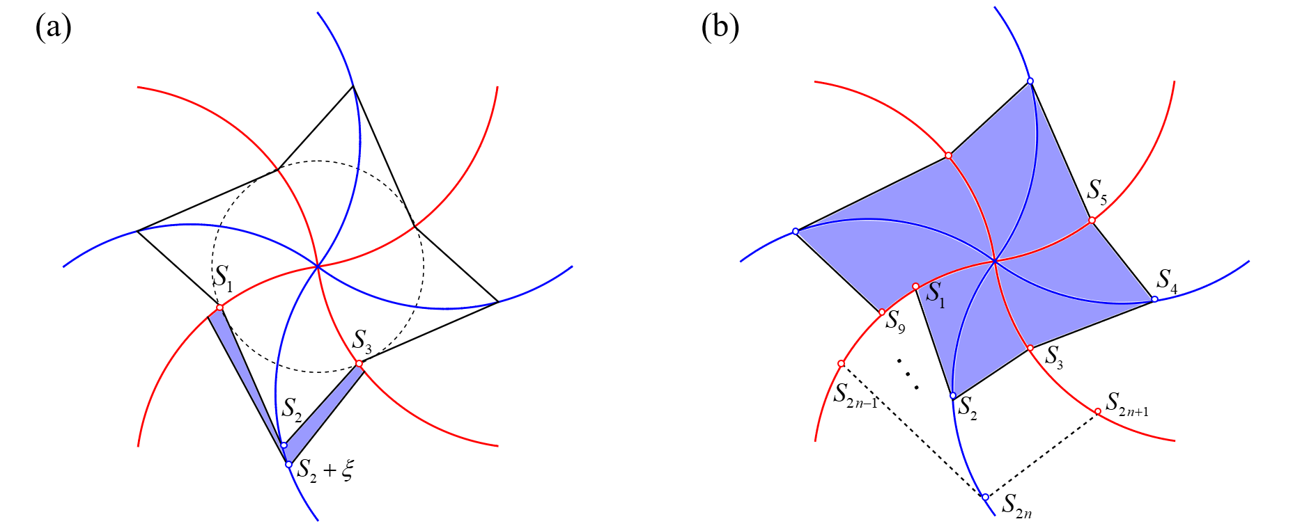
Some works have discussed the generator distribution in a single developable surface (Solomon et al., 2012; Chen et al., 2022). As for origami panels, the geometric constraints between folds and panels induce a more complex generator distribution. The generators are classified based on their starting and ending points, and panels are divided into different segments as shown in Fig. 2(a). Such classification is essential for elastic energy analysis in the following sections. Focusing on smooth developable folds, the properties and distinctions of different domains are analyzed as follows.
Crease-edge domain. In this domain, generators start at creases and end at edges. In previous works concerning a narrow strip, the crease-edge domain covers the whole panel.
Edge-edge domain. In this domain, generators start and end at edges. When no external loads are applied on the panel, the edge-edge domain remains planar to satisfy the balance of moments.
Plane domain. If the generator distribution function jumps, an infinite occurs on crease. According to Eq. (11), it leads to . Geometrically, it represents the situation where two generators intersect at one point on the crease, forming a plane domain. We then discuss possible situations that cause the jump in . We assume remains continuous over each panel and remains finite along the fold. Otherwise, the discontinuity will induce an infinite curvature and unphysical divergent bending energy. For developable folds, Eq. (13) is converted into
| (15) |
Analysing Eq. (15), we give all possible situations that form jumps in and plane domains.
-
1.
and remains finite. From Eq. (15), since and remain finite, the infinite leads to an infinite , which results in a discontinuity of Frenet normal . Notice that from the geodesic curvature constraint we derive
(16) then a discontinuity in breaks this constraint, since remain continuous. Therefore, such a situation cannot occur.
- 2.
-
3.
In this case, jumps and a plane domain forms. and may jump as well, and to avoid panel intersections, the jump of at the jumping point satisfies and , constraining , and .
In summary, a plane-plane domain forms in the following two situations: (1) and with ; (2) .
Crease-crease domain. In this domain, the generators start from one crease and end at the same crease. At a limiting point , the length of the generator tends to zero, where and jumps rapidly from to . In the following discussion we discuss how generator distribute in panel . To derive the generator distribution function , we focus on an infinitesimal region around and define , , , and with . Due to possible singularities in Eq. (15), is given by analyzing the the order of the parts , and in Eq. (15).
We start with the order of , which is derived from
| (17) |
Considering smooth folds, is finite. Therefore, . Thus we derive
| (18) |
To keep the principle curvature finite, an infinite derived from Eq. (17) should keep finite. Therefore, is at most . We then derive
| (19) |
From Eq. (15), (17), (18) and (19), the order of is derived
| (20) |
which leads to
| (21) |
Therefore, in panel jumps from to rapidly. To avoid the intersection of generators in panel , panel must be divided into two pieces at . To help understand this conclusion we give a simple example of curved origami with crease-crease domain. As demonstrated in Fig. 2(b), a semi-circle fold is folded into
| (22) |
Consequently, a nontrivial deformation may exist when the crease-crease domain appears in panel (red domain in Fig. 2(b)), but the other panel (blue domain in Fig. 2(b)) will separate at point to avoid the intersection of generators.
Crease-crease generators also bring extra geometric constraints between linked points. Suppose that a generator starting from ends at (as illustrated in Fig. 2(a)), from we derive that is a function of .
2.3 Mechanics of single-curve-fold origami
As a conclusion of Section 2.1, the deformation of curved origami depends on the curvature and torsion of the crease. However, in practical scenarios, controlling the curvature and torsion at every point on the crease is impractical. Instead, the folding procedure is conducted by adding mechanical loads or geometric constraints. The mechanical properties of the crease and panels thus play a significant role in the process, and the equilibrium equations of single-curve-fold systems can be derived via energy analysis.
2.3.1 Energy distribution in single-curve-fold origami
The elastic energy of curved fold origami consists of folding energy concentrated on creases and bending energy distributed in panels. For folding energy, we assume that folds are modeled as linear elastic torsional springs with direction . The energy of the fold between is expressed as
| (23) |
where is the torsional stiffness per unit length, and is the line energy density of the crease. From Eq. (14), is a function of
| (24) |
For bending energy, the surface energy density at of a bending developable surface is proportional to derived in Eq. (13). Therefore the bending energy between generators starting from and is
| (25) | ||||
where is the equivalent line density of bending energy after dimensional reduction and is the bending modulus of the panel. Note that , the projection of the generator length vector onto , is determined by along with the reference configuration and remains invariant during isometric deformation, therefore from Eq. (13), is generically expressed as
| (26) |
which indicates how bending energy correlates with the geometry of the deformed curve.
For different domains defined in Section 2.2, the bending energy integral is slightly different. Since the bending energy in the edge-edge domain and the crease-crease domain is calculated twice when integrating along the crease or the edge, the equivalent line density energy is augmented to
| (27) | ||||
where and represent the arclength parameter of the crease-crease, crease-edge, and edge-edge domain, respectively. Taking together the integral of along the crease and the edge-edge segment yields the bending energy of the whole panel. Therefore, the total elastic energy of the curved fold origami is
| (28) |
Additionally, we define
| (29) |
as the line density of elastic energy for the crease-dependent domain. In conclusion, the energy of single-curve-fold origami systems is expressed as a one-dimensional integral of the function determined by of folds and edges. The variation of energy reads the equilibrium equations that govern and of the deformed curve, which will be derived later.
2.3.2 Equilibrium equations for freely deformed systems
We start with the simplest situation where no geometric constraints and mechanical loads are applied to the system. Practically, it describes how an origami structure naturally relaxes to a nonplanar configuration. Note that the edge-edge domain keeps planar when no external loads are added to the panel. Then, the system is only crease-dependent.
For origami only with the crease-edge domain, the variation of the energy over and at equilibrium satisfies
| (30) | ||||
The variational principle indicates the Euler-Lagrange equations and along the crease, where
| (31) | ||||
and the boundary conditions , , on both ends .
Considering the crease-crease domain, the corresponding points at the crease on the same generator have additional geometric constraints (Fig. 2), i.e., only one point is free. Let the segment of the crease-crease domain be given by the arclength interval with a limiting point in between. The integral domain of the total energy can be reduced from to , given by
| (32) |
where
| (33) |
and the Euler-Lagrange equations follow, where
| (34) | ||||
2.3.3 Equilibrium equations for systems with geometric constraints
In other cases, curved folding is conducted by applying geometric loads at both ends of the crease, such as fixing and or giving closeness condition . Since no mechanical loads are applied on the panels, no edge-edge domain participates in the deformation, and the system is crease-dependent. The equilibrium state is also derived using the minimum total potential energy principle. The geometric constraints will introduce Lagrangian multipliers and thus make the Euler-Lagrange equations different from Eq. (31). However, many geometric constraints, including the displacement constraints, are not convenient to be expressed as functions of and . Instead, we variate by giving a virtual displacement of the crease. and are then written as
| (35) | ||||
in Eq. (30) is then converted into
| (36) |
where stands for boundary values and satisfies the extensibility condition for the crease . Integrating Eq. (36) by parts, we have
| (37) |
However, , and are not totally independent. This can be seen by noting that
| (38) |
and therefore
| (39) |
for any given . Combining and using Eq. (39), Eq. (36) is converted to
| (40) |
where
| (41) | ||||
with given by Eq. (31) for crease-crease domain or (34) for crease-edge domain. The variation method using virtual displacement equivalently changes the variable from arc length parameter to the vector coordinate , and the geometric constraints are then transformed into boundary conditions. Therefore, to make Eq. (40) satisfied for any , the Euler-Lagrange equations under geometric constraints are .
As a special case, a closed smooth crease automatically satisfies all the boundary conditions, since the variations of the vectors at and are equal, leading to . For systems with small torsion, narrow panels and large crease stiffness, i.e., and , Eq. (41) degenerates to the equilibrium equations derived in previous work concerning folded annular strips (Dias et al., 2012).
In summary, we develop a general framework for understanding the deformation of single-curve-fold origami with arbitrary reference shapes in various mechanical scenarios.
3 Multi-curve-fold origami theory
Based on the single-curve-fold origami theory derived in Section 2, we move to multi-curve-fold origami. One unique geometric property of multi-curve-fold origami is that the deformation of one fold directly influences the neighboring folds. Therefore, multi-curve-fold origami cannot be theoretically modeled as simple combinations of single-curve-fold origami. In this section, we start with analyzing geometric correlations between folds to derive the geometric mechanics of multi-curve-fold origami.
3.1 Geometric correlations between curved folds
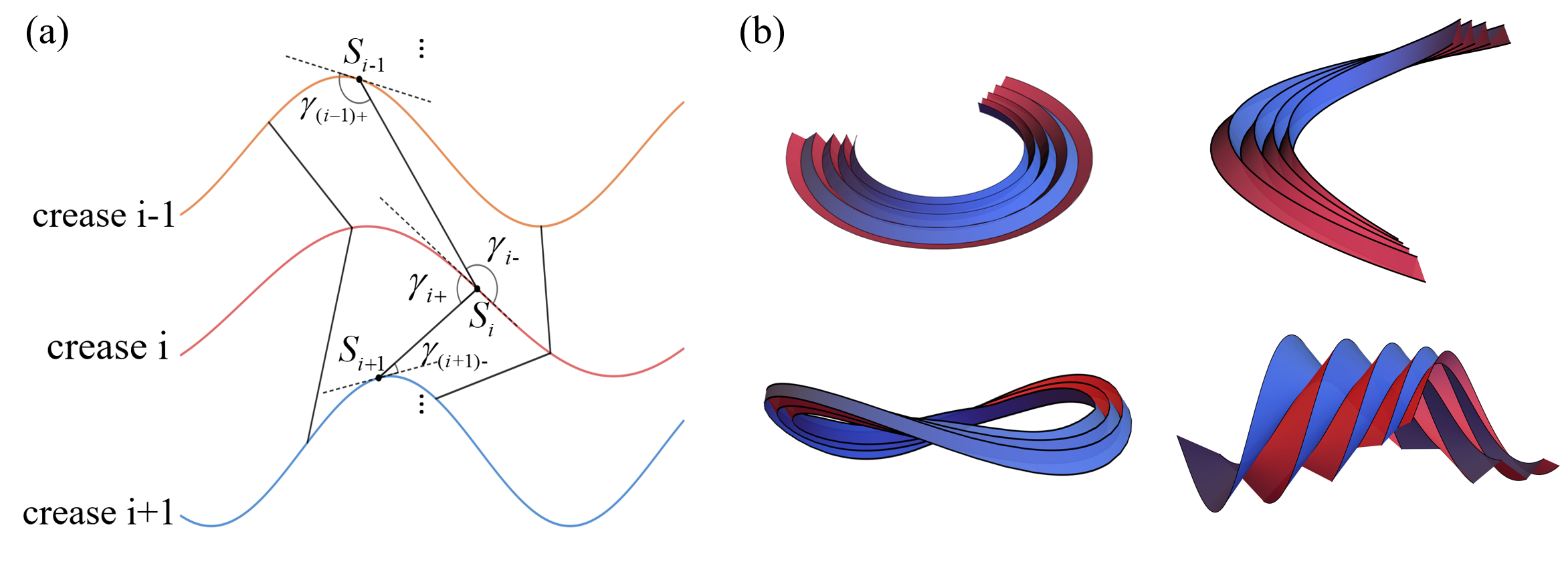
The geometric correlations are built by generators connecting different folds. Suppose that the two generators start at point on crease and end at point on crease and point on crease -1, as shown in Fig. 3(a). When the reference shapes and crease patterns are given, are determined by and , the angle between the crease and the generator. features the generator distribution by
| (42) |
Therefore, , and are expressed in terms of and when the reference shape and crease pattern are given
| (43) | ||||
Besides, the correlation of is given by
| (44) |
which introduces the correspondence of between the neighboring creases as
| (45) |
From Eq. (13), and are expressed as functions of and , therefore the geometric correlations between neighboring creases can be generally represented in terms of the crease curvature and torsion
| (46) | ||||
where . Here, the theory is only applicable to the domains that are covered by continuously connected generators between creases.
The propagation of deformation can be visualized in numerical experiments in the following steps. (1) From the given curvature and torsion, the Frenet frame fixed to the crease (defined as crease ) is derived, and the generator distribution on panel is solved from Eq. (13). (2) Darboux frame is then obtained, leading to the parametric equation of panel and crease . (3) Recursively, we can plot the deformed configuration of parts related to the given crease. In some cases where Eq. (50) can not be explicitly solved, discrete differential geometry is used in the procedure (Bobenko and Suris, 2008; Müller and Vaxman, 2021). The results of four numerical experiments are shown in Fig. 3(b). This numerical method contributes to the geometric design of curved origami with multiple creases.
3.2 Mechanics of multi-curve-fold origami
For structures with multiple creases, its elastic energy consists of the folding energy of creases and the bending energy of panels
| (47) |
The bending energy of panel , , and the folding energy of crease , , are given by
| (48) | ||||
where and are derived in Eq. (23) - (26). The system reaches its stable state when the energy minimizes under the constraints expressed in Eq. (46). With proper boundary conditions, the whole panels are covered by continuously connected generators. The curvature and torsion of crease are derived from Eq. (46)
| (49) |
and from Eq. (24) and (26), Eq. (47) is simplified into
| (50) |
According to principles of variation, we obtained the Euler-Lagrange equations for structures without geometric constraints, where
| (51) | ||||
Following Eq. (35) - (41), the Euler-Lagrange equations for systems with geometric constraints can be derived
| (52) | ||||
where and are given by Eq. (51).
3.3 Deformation of curved origami with annular folds
In this section, we theoretically explain how curved origami structures with annular folds deform within the framework established previously. The equilibrium configuration minimizes the total elastic energy (folding energy + bending energy) and results in a buckled structure with nonzero torsion.
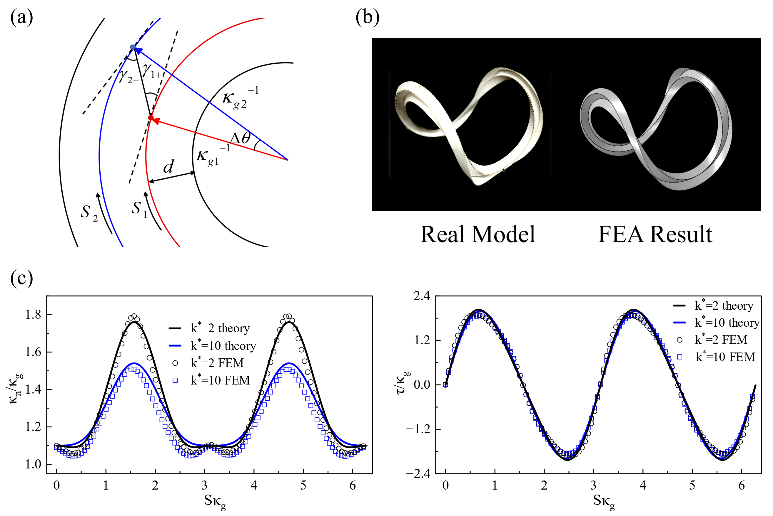
Suppose that a generator starts from and ends at , as shown in Fig. 4(a). The geometric correlations are given by
| (53) | ||||
Thus are derived as functions of (). From Eq. (46), (48) and (50), the energy of the system is derived
| (54) |
Substituting into Eq. (51) and (52) yields the equilibrium equations of the system.
Due to the difficulty in numerically solving the full equilibrium equations, we derive an approximate result using the perturbation theory inspired by previous work concerning curved origami with single annular fold (Dias et al., 2012), which predicts the amplitude of the normal curvature () and the torsion distribution. Here we use our generalized energy distribution and keep a higher order term in to reach a better prediction in multi-curve-fold origami. We assume the inner fold has and . From the zeroth order Euler-Lagrange equations, satisfies
| (55) |
where is the non-dimensionalized stiffness, chosen to be equal on crease and . is the strip width and is the rest angle of folds. The closeness of the fold yields a coupling between and , which is satisfied by choosing an appropriate . We then vary to minimize the energy, while is chosen to satisfy the initial value of .
We compare the results obtained from the theory and finite element analysis (FEA). The finite element modeling of curved origami is mainly discussed in Section 4.4.1, and the qualitative comparison between the FEA result and the real model is shown in Fig. 4(b), indicating that FEA captures the buckling phenomenon well. To illustrate that both geometry and elasticity contribute to the deformation, we calculate two cases with that have the same initial value of ensured by choosing the rest angle is changed to ensure that the initial values (). The geometric coefficient is selected as . The quantatative comparison between theoretical and FEA results of are shown in Fig. 4(c), where we define for convenience. The results show that the approximate theory predicts the distribution of torsion and curvature well, which explains the buckling phenomenon. To obtain the solutions of more precisely, the higher order terms () are needed. The results also illustrate that despite the same initial values of , the elastic coefficients affect the deformations in the whole field, which is quite different from the single-vertex multi-curve-fold origami that will be discussed shortly.
4 Single-vertex multi-curve-fold origami theory
Among various multi-curve-origami structures, there is a special type with multiple curved folds intersecting at one vertex. Despite a large number of single-vertex curved origami, such as those in plants (Cheng et al., 2023) and art design (Mitani, 2019), the theories predicting the deformation still lack. In this section, we introduce the extra vertex constraints to the theories in previous sections and develop the theory for single-vertex curved origami, unveiling a universal equilibrium configuration in the region near the vertex. Numerical simulations are performed to validate the theory.
4.1 Geometric constraints in single-vertex origami
We start by converting Eq. (43) and (46) into explicit forms adaptable to single-vertex curved origami. As shown in Fig. 5(a), the correlations between polar coordinates points connected by generators are expressed as
| (56) |
where is the crease in polar coordinates. From Eq. (45) and (46) revealing geometric correlations between adjacent folds, the crease curvature and torsion of the two points satisfy
| (57) |
| (58) |
where . For folds with constant geodesic curvatures, define , and Eq. (56) is explicitly solved by
| (59) | ||||
Considering the N-fold case, the single-vertex curved origami is constrained by the closeness conditions
| (60) | ||||
which restrict the creases’ configuration spaces. For the axisymmetric deformation, the symmetry condition also needs to be satisfied
| (61) | ||||
The tangent vectors of folds intersecting at a vertex lead to extra geometric constraints of the folding angles at , as shown in Fig. 5(b). We assume that generators cannot intersect at the vertex, otherwise the bending energy diverges. Under the assumption, stays during isometric deformation. We define , and according to the previous work on single-vertex origami with straight folds (Evans et al., 2015), , the folding angle of creases at the vertex, are expressed in forms of as
| (62) | ||||
Therefore are independent. Incorporating the rotational symmetry, Eq. (62) are simplified as
| (63) |
which reveals the geometric correlations between the initial folding angles of mountain folds and valley folds.
4.2 Near-field deformation
In Section 4.1, we indicate that the vertex introduces extra periodic constraints (Eq. (60) and (61)) and folding angle constraints (Eq. (62) and (63)), distinct from multi-curve-fold origami without a vertex. Next, we demonstrate that the periodicity at the vertex and the geometric constraints between neighboring creases will bring strong limitations on the configuration space of the origami, leading to distinct behaviors in the near field and far field defined below.
Near field. The near field is defined as the region near the vertex with limited configuration space. The analytical classification will be given below.
Far field. The far field is the complement of the near field in the origami structure. In this domain, no correlations between creases occur and the configuration space is free.
To study the behaviors in these two domains, we first prove a theorem about the equilibrium configuration in the near field. Then we will derive the exact boundary between these two fields in Section 4.3 and study the far-field deformation. Suppose that the two generators starting from on crease 2 end at and on crease and crease , as shown in Fig. 6(a). The relatively concise theorem on the near-field deformation is based on the following two lemmas.
Lemma 1.
If as illustrated in Fig. 6(a), the curvature and torsion distribution and in a finite neighborhood of can be derived from and .
Proof.
To guarantee the periodicity constraints, and are satisfied everywhere on crease and crease 3 with every . According to Eq. (56) - (58), the n-th order periodicity constraints can be written as
| (64) | ||||
where .
From , we first derive . Given , can be derived by Eq. (56) and (57), and then can be derived from . Inductively using Eq. (64), and are derived. The curvature and torsion on the neighboring points are then expressed as
| (65) |
Notice that as , with finite . Thus Lemma is proved. Therefore, the geometry of point determines the deformation of a finite domain, marked in Fig. 6. ∎
Lemma 2.
If as illustrated in Fig. 6(b), the distribution of and in the whole near field can be derived from the distribution of and on .
Proof.
We assume that . As shown in Fig. 6(b), if the geometry on of crease 2 is given, the geometry on of crease 3 is determined according to Eq. (57) and (58). The geometry on of odd folds then determines the geometry on of even folds. The conduction will extend the geometry-determined domain, which continues until . Then we use Lemma 1 to extend the geometry-determined region, and the procedure continues until a generator reaches the boundary of the structure. ∎
Based on the above two lemmas, the theorem of the near-field deformation can be proved as follows.
Theorem 1.
The near-field deformation of a single-vertex curve-fold origami only depends on the curvature at the vertex.
Proof.
From Eq. (63), we may derive and when is given. Since the projection length of generators at the vertex, the geometric constraints Eq. (64) in Lemma 1 are simplified to
| (66) | ||||
when . Therefore, as a conclusion of Lemma 1, the distribution of and on a finite range is determined by . As a result of Lemma 2, the entire near-field deformation can be derived, which is related to . ∎
The theorem indicates that, given the curvature at the vertex, the near-field deformation is independent of other mechanical properties. Moreover, the theorem implies a way of describing the near-field deformation concisely. Specifically, the geometry of the curve-fold origami can be approximately demonstrated by
| (67) |
For folds with constant geodesic curvature, the coefficients of the series are easily derived via substituting Eq. (57) - (59) into (66).
The near-field theory can be easily generalized to origami with arbitrary curved creases , not limited to circular arcs. Specifically, Eq. (56) is generalized to
| (68) |
where and are the corresponding parameters at the generator connecting two neighboring creases. We could then compute at the vertex from Eq. (68). The coefficients of the series are thus derived from Eq. (66) to obtain the deformation of the full domain. Furthermore, the symmetric deformation condition Eq. (61) can also be relaxed. Notice that the closeness condition Eq. (60) will bring intrinsic periodicity. We may follow similar steps to prove the near-field theory. However, in the asymmetric case, is not sufficient. Instead, the higher order terms are needed.
4.3 Far-field deformation
In Lemma 2, we show that the deformation is determined by the near-field theory until a generator ends at an edge. In other words, the generator distribution determines the boundary between the near-field domain and the far-field domain. Figure 7 shows two possible generator distributions that are distinguished by the relationships between and .
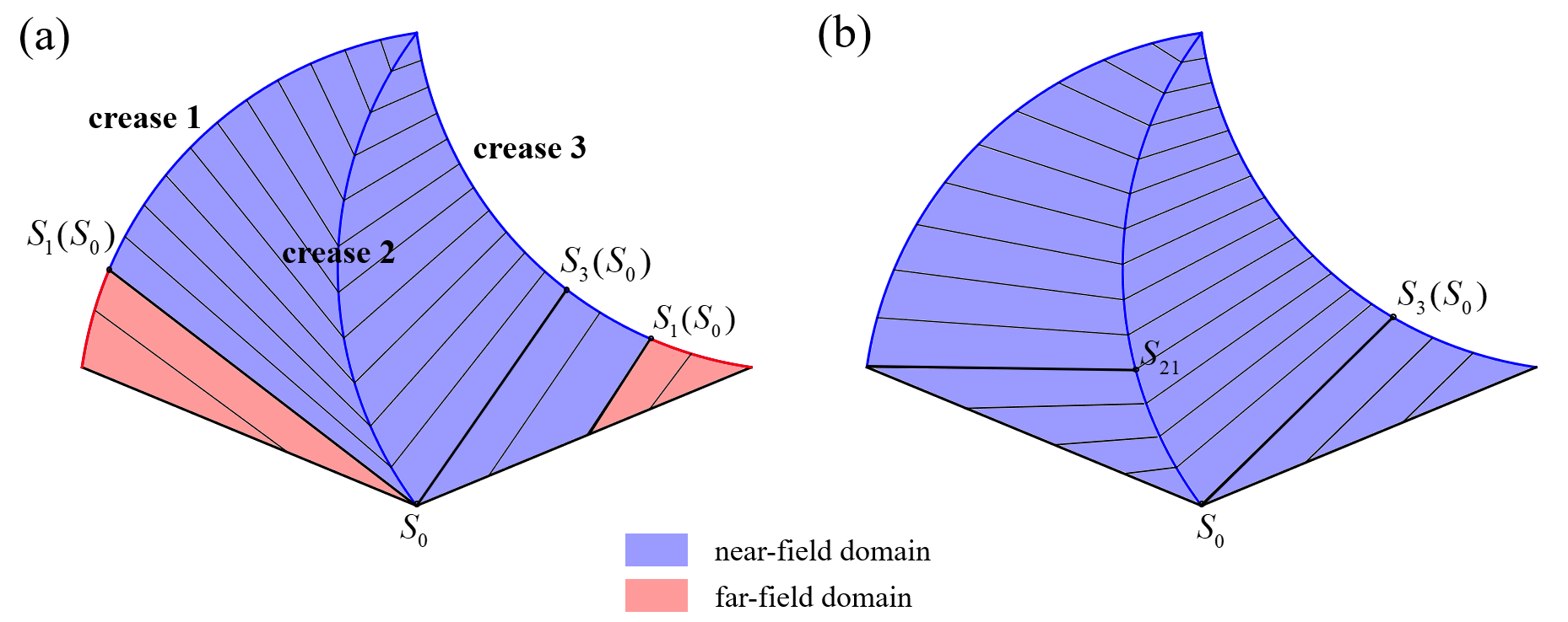
Situation A. As shown in Fig. 7(a), we have and . Therefore, all generators starting from crease (defined in Fig. 7(a)) on both panels end at the neighboring creases, leading to the conclusion that segment on crease 2 and segments on crease and 3 are determined by the near-field theory. The near-field and far-filed domains can be identified.
The deformation for Situation A can be derived as follows. Given , the boundary and the corresponding values are determined by the near-field theory. The deformation of the far-field region is then solved via energy minimization. For the systems without geometrical loads, the far-field regions deform freely, following Eq. (31) and the initial values . For systems with geometrical loads, is determined by the near-field theory, and the far-field deformation is thus given by Eq. (41).
Situation B. As shown in Fig. 7(b), we have and . Assuming that , the segment on crease satisfies the near-field theory. The segments on crease and are then determined, leading to the conclusion that the whole structure is determined by the near-field theory.
With both near-field and far-field theory, the deformation of single-vertex curved origami is derived. As for the situation with and , it is included in situation A by selecting crease or crease as the new crease . Situations with and are included in situation B due to symmetry. Therefore, the two cases include all possibilities. As a conclusion, If generators distribute continuously, at least one fold (crease ) is completely in the near-field domain.
4.4 Finite element modeling and numerical results of single-vertex curved origami
Numerical simulations of single-vertex curved origami are employed in this section to validate the single-vertex curved origami theory.
4.4.1 Finite element modeling of curved fold origami
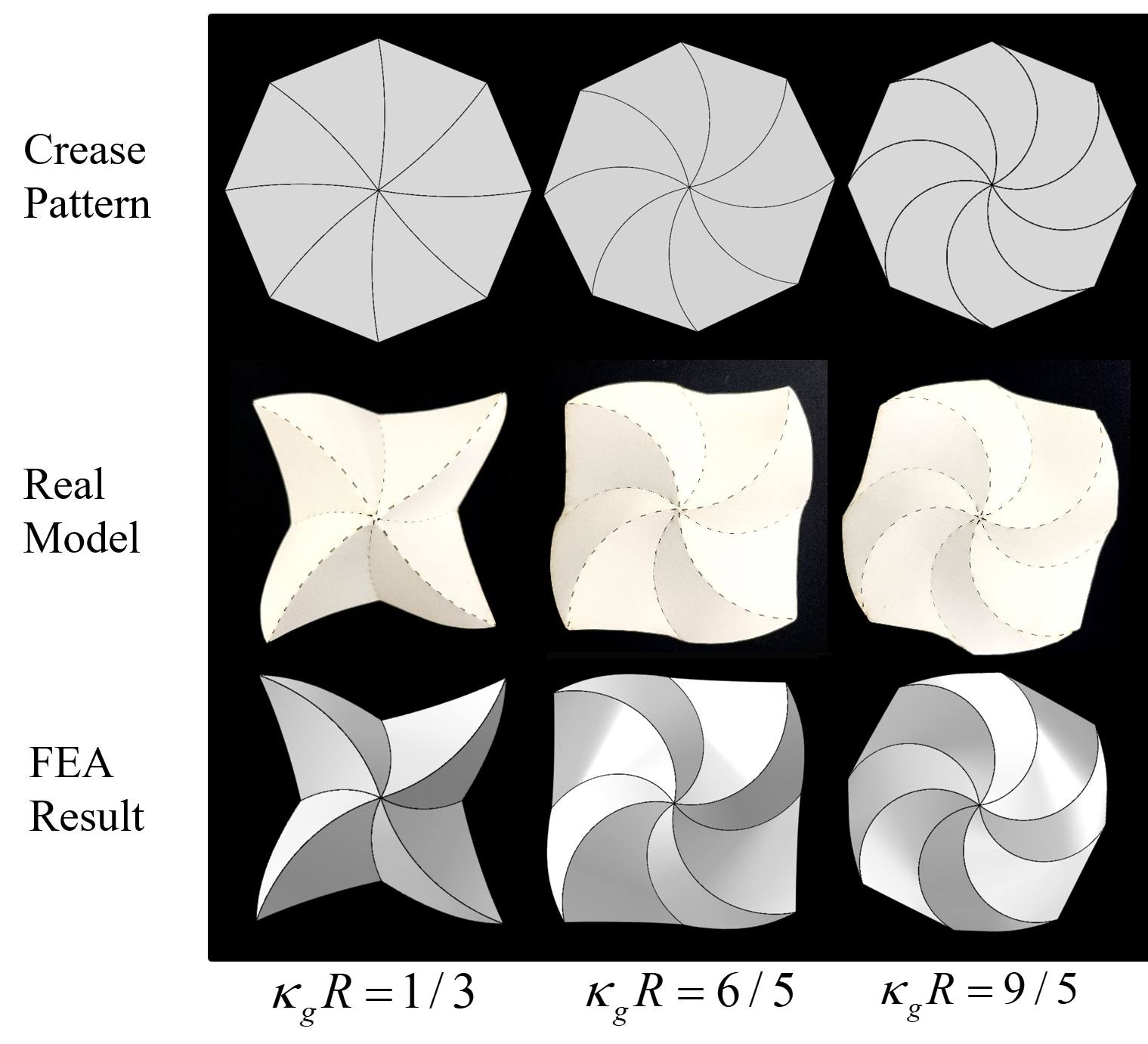
In finite element analysis, the origami panels are modeled as shells, and the elastic folds are modeled as discrete torsional springs (Woodruff and Filipov, 2018; Flores et al., 2022). In the following analysis, we generate finite element models using the commercial software Abaqus. The origami panels are modeled as S4R shell elements. The curved folds are modeled as join-rotation connectors with stiffness along the tangent of the folds, where is the fold length and is the number of nodes on each fold. The rest angle of curved folds is implemented by adding a connector moment of to the connectors on mountain and valley folds. We then simulate the deformation of the single-vertex curved origami with different crease patterns. The qualitative comparison between FEA results and real models is shown in Fig. 8, illustrating good agreement. represents the distance between the starting and ending points of the creases.
4.4.2 Comparison between theoretical solutions and numerical results
Here we compare the normal curvature and the torsion distribution of folds derived from theory and FEA. In FEA, the coordinates of the deformed folds are extracted to compute the discrete curvature and torsion. In the following situations, if crease is selected as the valley fold, we have derived from the near-field theory. As predicted in Section 4.3, the deformation of the valley folds is completely determined by the near-field theory, which will be examined in the following comparisons. To validate the universality of the near-field theory in Section 4.2, we compare the near-field solutions with numerical results of the folds, where we define and the variables are non-dimensionalized to . The following situations are discussed.
Folds with different . We model the arc-fold structures with different geodesic curvatures , and take the rest angles such that the deformed configurations have the same vertex folding angles . Figure 9(a) shows that the theoretical and FEA results reach good agreement in most of the near-field domain.
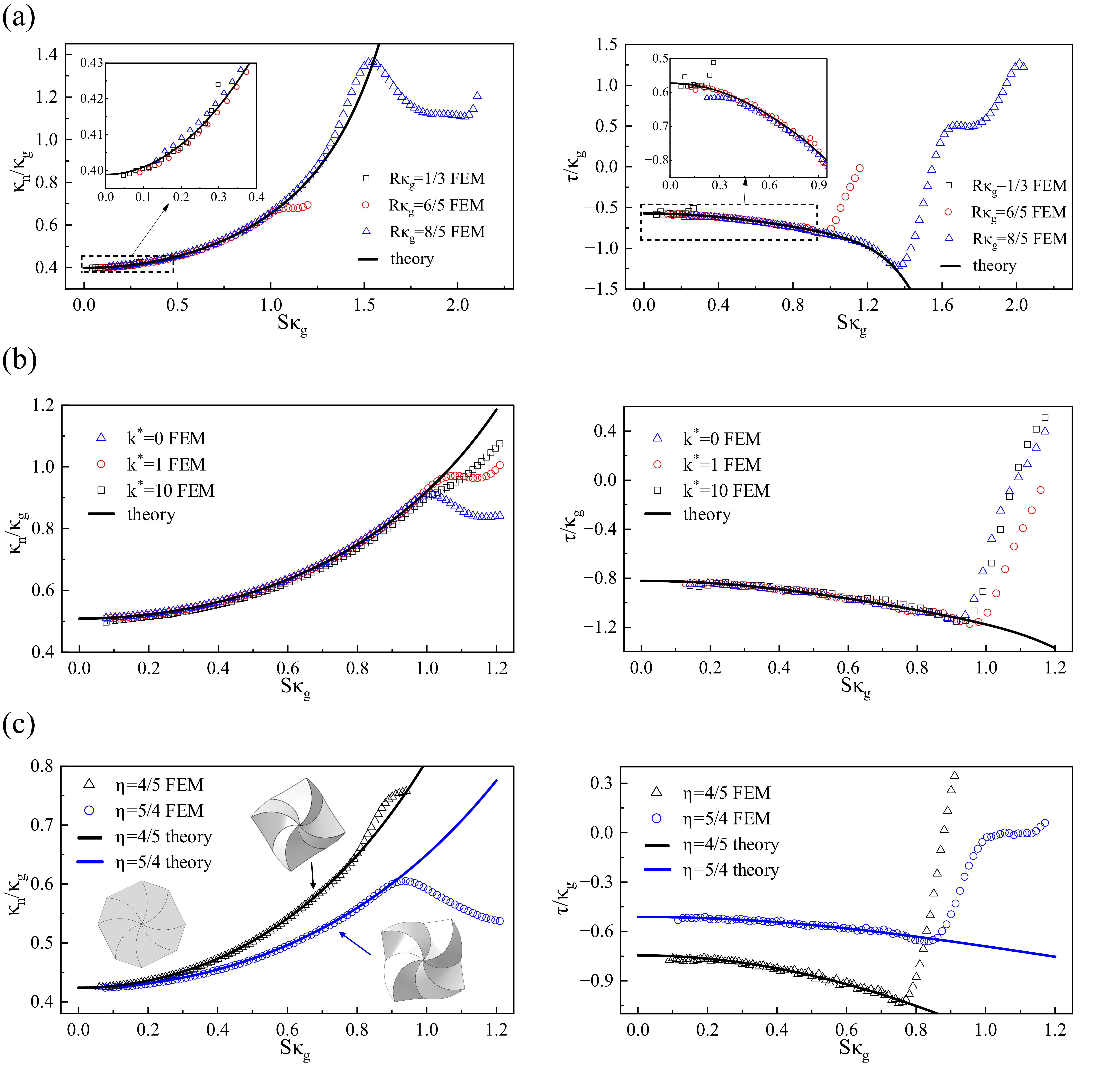
Folds with different . We model arc-fold structures with different non-dimensionalized stiffness . For , the folding process is simulated by giving the rest angles , while folding structure with zero is achieved via applying a vertical load at the vertex. The results in Fig. 9 validate that the deformations are independent of elastic coefficients in a large range once the initial folding angle is given.
Folds with distinct neighboring . We model the structures with distinct neighboring geodesic curvature , where . Let be the ratio between the geodesic curvatures of the mountain and valley folds. Here, we simulate the cases that have and , by applying vertical displacements at vertices. The vertical displacements are chosen to make the initial folding angles identical for the two cases. The results in Fig. 9(c) illustrate that the near-field theory works well in a large range.
The above results validate that the near-field solutions Eq. (67) derived from Eq. (66) reach satisfactory agreement with simulations for various situations. It indicates that the near-field deformation is solely dependent on the initial value and is independent of the geodesic curvatures, elastic coefficients and deforming processes. In contrast, the deformation of multi-curve-fold origami without vertices is governed by the Euler-Lagrange equations, which relies on the elastic coefficients, as shown in Section 3.3. We prove in Section 4.2 that, the significant difference owes to the periodicity at the vertex. However, a little unsatisfactory part remains. As analyzed in Section 4.3, the deformation of the valley fold should be completely determined by the near-field theory if the generators distribute continuously, but Fig. 9 shows disagreement at the end of the folds. We discuss this observation further in the next section.
4.4.3 Further discussion on the far-field solutions
We anticipate that the discontinuities in and cause the deviation between FEA and theoretical results in Fig. 9. As discussed in Section. 2.1, discontinuities occur when and jump, which will form a planar domain. The new generator distribution is shown in Fig. 10(b), which is chosen to satisfy the energy density contour in Fig. 10(a). Such distribution only occurs when the periodic symmetry slightly breaks, since it contradicts with Lemma 2 proved based on a strictly satisfied periodicity. The good agreement in the near-field region indicates that we may assume the broken symmetry does not affect the low-order (depends on ) coefficients of the near-field solutions. Therefore, on and , and are determined by the near-field theory, but the geometry on cannot be determined by the geometry on due to the symmetry breaking. Since is continuous at and is continuous at , from Eq. (13) the geometric coefficients near and satisfy
| (69) | ||||
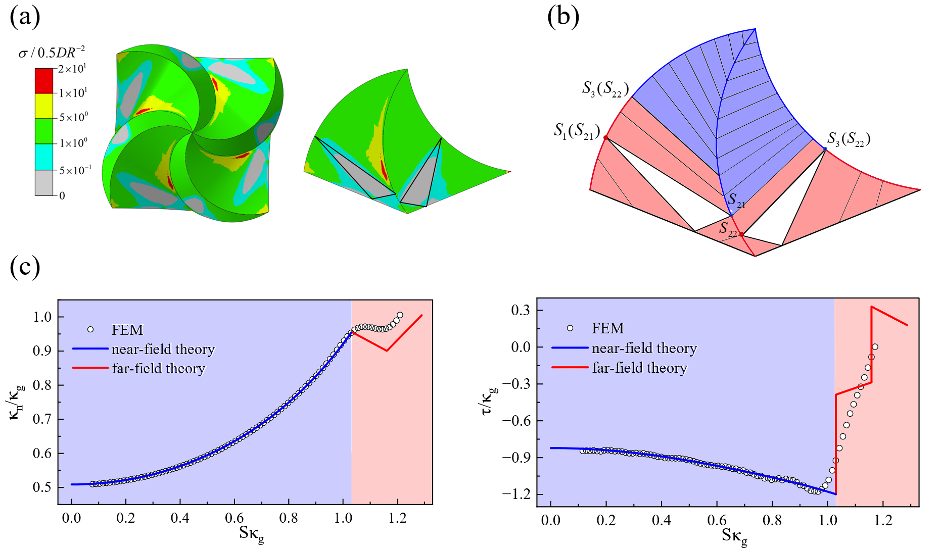
From the energy density contour and the results in the previous subsection, we assume that for the case , discontinuities on crease occur at and . and are then derived from the near-field theory, since numerically we observe that changes in high-order terms affect little to both on and on . The jumps in and should minimize the bending and folding energy of the far field, where the bending energy of crease-edge domains is given by Eq. (25), with the projection length of generators computed as
| (70) |
To give a first approximate solution for the far-field deformation, we assume that in the far field, of mountain and valley folds are linear in arclength. For , the bending and folding energies are comparable, therefore we assume that the changes in bending and folding energies caused by the jump in cancel each other, and the change in generator distributions, i.e., , dominates the total energy change. Specifically, the jumps of should minimize the zero-order energy given by the multiplication of area and energy density at a single point
| (71) |
where represents the surface area of the crease-edge domain, which is determined by in Eq. (70) once is given. In zero-order energy, we assume
| (72) |
Thus the ratio can be derived from the near-field theory. Since generators starting from and form a triangle, couples with . Similarly couples with . We could then derive via separately minimizing the energy on the two panels. From Eq. (13) and (69), the jump of satisfies
| (73) |
Therefore, with derived by energy minimization, at and is derived. According to the linear assumption, the far-field curvature is then given approximately. The jumps of are given as well. in is given by Eq. (13)
| (74) |
where is given by the revised far-field theory and is given by the near-field theory. On , is chosen to approximately minimize the energy of the segment. Fig. 10(c) shows the comparison between the theoretical and numerical results, validating the revised far-field theory. The geometrical and elastic properties of the structure are .
5 Conclusion
In this work, a comprehensive framework for multi-curve-fold origami is established. This framework theoretically explains how geometry and elasticity determine the deformation of curved fold origami structures. As an example of multi-curve-fold origami with periodicity, the theory of single-vertex curved origami is established, unveiling a striking vertex-constrained universal equilibrium configuration. Our main contributions are summarized as follows:
(1) We characterize all possible generator distributions and the corresponding energy distributions in single-curve-fold origami with wide panels. We then derive the equilibrium equations that predict how single-curve-fold structures with arbitrary reference tiles deform via energy minimization. Our theory removes the limitations on the panel width and generator distribution.
(2) We derive the geometrical correlations between neighboring creases in multi-curve-fold origami. Based on this, we extend the single-curve-fold origami theory to the multi-curve-fold origami theory. The theory is used to solve the deformation of curved origami with annular creases. Numerical simulations validate the theory.
(3) We derive the single-vertex curved origami theory. We prove that the periodicity at the vertex strongly constrains the configuration space, yielding a universal equilibrium shape at the near-field domain, regardless of the mechanical properties. In contrast, the far-field theory, derived by energy minimization, is dependent on the mechanical properties. Numerical simulations are conducted, showing good agreement with theoretical predictions.
We believe that our generalized multi-curve-fold origami theory, including the vertex-constrained universality, can extend the understanding of the physics of the curved origami system and provide new insights into the shape programming. We anticipate that our work can contribute to the design of complex curved origami structures in the fields of robotics, metamaterials and architectures.
CRediT authorship contribution statement
Zhixuan Wen: Conceptualization, Methodology, Software, Validation, Formal analysis, Writing – original draft. Pengyu Lv: Methodology, Writing– review & editing. Fan Feng: Conceptualization, Investigation, Methodology, Software, Writing– review & editing. Huiling Duan: Conceptualization, Methodology, Writing – review & editing, Supervision, Project administration, Funding acquisition.
Declaration of competing interest
The authors declare that they have no known competing financial interests or personal relationships that could have appeared to influence the work reported in this paper.
Data availability
No data was used for the research described in the article.
Acknowledgement
References
- Audoly and Van der Heijden (2023) Audoly, B., Van der Heijden, G., 2023. Analysis of cone-like singularities in twisted elastic ribbons. Journal of the Mechanics and Physics of Solids 171, 105131.
- Baek et al. (2020) Baek, S.M., Yim, S., Chae, S.H., Lee, D.Y., Cho, K.J., 2020. Ladybird beetle inspired compliant origami. Science Robotics 5, eaaz6262.
- Bobenko and Suris (2008) Bobenko, A.I., Suris, Y.B., 2008. Discrete differential geometry: integrable structure. volume 98. American Mathematical Soc.
- Chen et al. (2022) Chen, Y.C., Fosdick, R., Fried, E., 2022. A novel dimensional reduction for the equilibrium study of inextensional material surfaces. Journal of the Mechanics and Physics of Solids 169, 105068.
- Cheng et al. (2023) Cheng, X., Fan, Z., Yao, S., Jin, T., Lv, Z., Lan, Y., Bo, R., Chen, Y., Zhang, F., Shen, Z., et al., 2023. Programming 3d curved mesosurfaces using microlattice designs. Science 379, 1225–1232.
- (6) Demaine, E.D., Demaine, M.L., Huffman, D.A., Koschitz, D., Tachi, T., . Characterization of curved creases and rulings: Design and analysis of lens tessellations. arXiv:1502.03191 .
- Demaine et al. (2011) Demaine, E.D., Demaine, M.L., Koschitz, D., Tachi, T., 2011. Curved crease folding: a review on art, design and mathematics, in: Proceedings of the IABSE-IASS symposium: taller, longer, lighter, Citeseer. pp. 20–23.
- Dias and Audoly (2014) Dias, M.A., Audoly, B., 2014. A non-linear rod model for folded elastic strips. Journal of the Mechanics and Physics of Solids 62, 57–80. Sixtieth anniversary issue in honor of Professor Rodney Hill.
- Dias and Audoly (2015) Dias, M.A., Audoly, B., 2015. “Wunderlich, meet Kirchhoff”: A general and unified description of elastic ribbons and thin rods. Journal of Elasticity 119, 49–66.
- Dias et al. (2012) Dias, M.A., Dudte, L.H., Mahadevan, L., Santangelo, C.D., 2012. Geometric mechanics of curved crease origami. Physical review letters 109, 114301.
- Dias and Santangelo (2012) Dias, M.A., Santangelo, C.D., 2012. The shape and mechanics of curved-fold origami structures. Europhysics Letters 100, 54005.
- Do Carmo (1976) Do Carmo, M.P., 1976. Differential geometry of curves andsurfaces. Englewood Cliffs, New Jersey .
- Duffy et al. (2021) Duffy, D., Cmok, L., Biggins, J.S., Krishna, A., Modes, C.D., Abdelrahman, M.K., Javed, M., Ware, T.H., Feng, F., Warner, M., 2021. Shape programming lines of concentrated Gaussian curvature. Journal of Applied Physics 129, 224701.
- Duncan and Duncan (1982) Duncan, J.P., Duncan, J., 1982. Folded developables. Proceedings of the Royal Society of London. A. Mathematical and Physical Sciences 383, 191–205.
- Evans et al. (2015) Evans, A.A., Silverberg, J.L., Santangelo, C.D., 2015. Lattice mechanics of origami tessellations. Physical Review E 92, 013205.
- Feng et al. (2024) Feng, F., Dradrach, K., Zmyślony, M., Barnes, M., Biggins, J.S., 2024. Geometry, mechanics and actuation of intrinsically curved folds. Soft Matter 20, 2132–2140.
- Feng et al. (2022) Feng, F., Duffy, D., Warner, M., Biggins, J.S., 2022. Interfacial metric mechanics: stitching patterns of shape change in active sheets. Proceedings of the Royal Society A 478, 20220230.
- Flores et al. (2022) Flores, J., Stein-Montalvo, L., Adriaenssens, S., 2022. Effect of crease curvature on the bistability of the origami waterbomb base. Extreme Mechanics Letters 57, 101909.
- Fuchs and Tabachnikov (1999) Fuchs, D., Tabachnikov, S., 1999. More on paperfolding. The American Mathematical Monthly 106, 27–35.
- Huffman (1976) Huffman, 1976. Curvature and creases: A primer on paper. IEEE Transactions on Computers C-25, 1010–1019.
- Jiang et al. (2019) Jiang, C., Mundilova, K., Rist, F., Wallner, J., Pottmann, H., 2019. Curve-pleated structures. ACM Transactions on Graphics (TOG) 38, 1–13.
- Karami et al. (2024) Karami, A., Reddy, A., Nassar, H., 2024. Curved-crease origami for morphing metamaterials. Phys. Rev. Lett. 132, 108201.
- Kilian et al. (2008) Kilian, M., Flöry, S., Chen, Z., Mitra, N.J., Sheffer, A., Pottmann, H., 2008. Curved folding. ACM transactions on graphics (TOG) 27, 1–9.
- Koschitz et al. (2008) Koschitz, D., Demaine, E.D., Demaine, M.L., 2008. Curved crease origami, in: Abstracts from Advances in Architectural Geometry (AAG 2008), Vienna, Austria. pp. 29–32.
- Lee et al. (2021) Lee, T.U., Chen, Y., Heitzmann, M.T., Gattas, J.M., 2021. Compliant curved-crease origami-inspired metamaterials with a programmable force-displacement response. Materials & Design 207, 109859.
- Lee et al. (2018) Lee, T.U., You, Z., Gattas, J.M., 2018. Elastica surface generation of curved-crease origami. International Journal of Solids and Structures 136, 13–27.
- Liu and James (2024) Liu, H., James, R.D., 2024. Design of origami structures with curved tiles between the creases. Journal of the Mechanics and Physics of Solids 185, 105559.
- Mitani (2011) Mitani, J., 2011. A design method for axisymmetric curved origami with triangular prism protrusions, in: Proceedings of 5th International Conference on Origami in Science, Mathematics, and Education (5OSME).
- Mitani (2019) Mitani, J., 2019. Curved-folding origami design. CRC Press.
- Mitani and Igarashi (2011) Mitani, J., Igarashi, T., 2011. Interactive Design of Planar Curved Folding by Reflection, in: Chen, B.Y., Kautz, J., Lee, T.Y., Lin, M.C. (Eds.), Pacific Graphics Short Papers, The Eurographics Association.
- Moulton et al. (2013) Moulton, D., Lessinnes, T., Goriely, A., 2013. Morphoelastic rods. part i: A single growing elastic rod. Journal of the Mechanics and Physics of Solids 61, 398–427.
- Mouthuy et al. (2012) Mouthuy, P.O., Coulombier, M., Pardoen, T., Raskin, J.P., Jonas, A.M., 2012. Overcurvature describes the buckling and folding of rings from curved origami to foldable tents. Nature communications 3, 1290.
- Müller and Vaxman (2021) Müller, C., Vaxman, A., 2021. Discrete curvature and torsion from cross-ratios. Annali di Matematica Pura ed Applicata (1923 -) 200, 1935–1960.
- Mundilova et al. (2023) Mundilova, K., Demaine, E.D., Lang, R., Tachi, T., 2023. Curved-crease origami spirals constructed from reflected cones, in: Holdener, J., Torrence, E., Fong, C., Seaton, K. (Eds.), Proceedings of Bridges 2023: Mathematics, Art, Music, Architecture, Culture, Tessellations Publishing, Phoenix, Arizona. pp. 401–404.
- Rabinovich et al. (2018) Rabinovich, M., Hoffmann, T., Sorkine-Hornung, O., 2018. Discrete geodesic nets for modeling developable surfaces. ACM Trans. Graph. 37.
- Rus and Sung (2018) Rus, D., Sung, C., 2018. Spotlight on origami robots. Science Robotics 3, eaat0938.
- Sadowsky (1930) Sadowsky, M., 1930. Theorie der elastisch biegsamen undehnbaren bänder mit anwendungen auf das möbius’ sche band. Verhandl. des 3, 444–451.
- Sasaki and Mitani (2022) Sasaki, K., Mitani, J., 2022. Simple implementation and low computational cost simulation of curved folds based on ruling-aware triangulation. Computers & Graphics 102, 213–219.
- Solomon et al. (2012) Solomon, J., Vouga, E., Wardetzky, M., Grinspun, E., 2012. Flexible developable surfaces. Computer Graphics Forum 31, 1567–1576.
- Starostin and van der Heijden (2007) Starostin, E.L., van der Heijden, G.H., 2007. The shape of a möbius strip. Nature materials 6, 563–567.
- Sun et al. (2024) Sun, Y., Song, K., Ju, J., Zhou, X., 2024. Curved-creased origami mechanical metamaterials with programmable stabilities and stiffnesses. International Journal of Mechanical Sciences 262, 108729.
- Tachi (2013) Tachi, T., 2013. Composite rigid-foldable curved origami structure. Proceedings of Transformables , 18–20.
- Tachi and Epps (2011) Tachi, T., Epps, G., 2011. Designing one-dof mechanisms for architecture by rationalizing curved folding, in: International Symposium on Algorithmic Design for Architecture and Urban Design (ALGODE-AIJ). Tokyo, p. 6.
- Todres (2015) Todres, R.E., 2015. Translation of w. wunderlich’s “on a developable möbius band”. Journal of Elasticity 119, 23–34.
- Woodruff and Filipov (2018) Woodruff, S.R., Filipov, E.T., 2018. Structural Analysis of Curved Folded Deployables. pp. 793–803.
- Wunderlich (1962) Wunderlich, W., 1962. Über ein abwickelbares möbiusband. Monatshefte für Mathematik 66, 276–289.
- Yu and Hanna (2019) Yu, T., Hanna, J., 2019. Bifurcations of buckled, clamped anisotropic rods and thin bands under lateral end translations. Journal of the Mechanics and Physics of Solids 122, 657–685.
- Zhang et al. (2023) Zhang, Z., Xu, Z., Emu, L., Wei, P., Chen, S., Zhai, Z., Kong, L., Wang, Y., Jiang, H., 2023. Active mechanical haptics with high-fidelity perceptions for immersive virtual reality. Nature Machine Intelligence 5, 643–655.
- Zou et al. (2024) Zou, Y., Feng, F., Liu, K., Lv, P., Duan, H., 2024. Kinematics and dynamics of non-developable origami. Proceedings of the Royal Society A 480, 20230610.