A family of thermodynamic uncertainty relations valid for general fluctuation theorems

Abstract

Thermodynamic Uncertainty Relations (TURs) are relations that establish lower bounds for the relative fluctuations of thermodynamic quantities in terms of the statistics of the associated entropy production. In this work we derive a family of TURs that explores higher order moments of the entropy production and is valid in any situation a Fluctuation Theorem holds. The resulting bound holds in both classical and quantum regimes and can always be saturated. These TURs are shown in action for a two level system weakly coupled to a bath undergoing a non time-symmetric drive, where we can use the Tasaki-Crooks fluctuation theorem. Finally, we draw a connection between our TURs and the existence of correlations between the entropy production and the thermodynamic quantity under consideration.

Introduction - In the recent decades, miniaturization has led to the development of devices and thermal machines operating in a nanoscopic scale Benenti et al. (2017); Li et al. (2012). These include quantum dots Josefsson et al. (2018), nano-junction thermoelectrics Dubi and Di Ventra (2011) and molecular motors Zhang et al. (2023); Kassem et al. (2017) to name a few. When considering the thermodynamics of these devices there are three important aspects of such systems. The first one is that contrary to macroscopic thermodynamic systems the fluctuations play an important role, so quantities like work and exchanged heat must be treated stochastically. Secondly, these systems are inherently out-of-equilibrium and so their operation entails some entropy production. Finally, these systems operate at a scale where quantum effects might have an important role and so a full quantum treatment is necessary for their study.

The effect that fluctuations have in a device is to make it more unreliable. For example, if during a particular run of an experiment the heat dissipation becomes significantly larger than average, then the device might be damaged or have its operation disrupted. On the other hand, a larger entropy production in a thermal machine leads to a reduced efficiency Pietzonka and Seifert (2018). A natural question is whether it is possible to reconcile small fluctuations with small entropy production by designing the device in a clever way. An important step in answering this question was the development of the Thermodynamic Uncertainty Relations (TUR) Barato and Seifert (2015); Pietzonka et al. (2016); Pietzonka and Seifert (2017); Pietzonka et al. (2017); Gingrich et al. (2016); Dechant (2018); Barato et al. (2018); Holubec and Ryabov (2018); Proesmans and Van den Broeck (2017). These are relations that relate the entropy production of the system with the relative fluctuations of currents in that same system through an inequality. The original TUR Barato and Seifert (2015) was formulated for classical Markovian systems and reads

$$\frac{\mathrm{Var}\left(J\right)}{\left\langle J\right\rangle^{2}}\geq\frac{1}{2\left\langle\Sigma\right\rangle}$$ (1)

where $J$ is a current integrated over time and $\Sigma$ is the corresponding entropy production. Note that because of the structure of the inequality, the entropy production imposes a lower bound to the relative fluctuations of $J$ and this bound diverges when the entropy production becomes smaller, meaning that there must always be a tradeoff between relative fluctuations and dissipation.

Fluctuation theorems (FT) Gallavotti and Cohen (1995); Jarzynski (1997); Crooks (1998); Piechocinska (2000); Tasaki (2000); Kurchan (2000); Jarzynski and Wójcik (2004); Andrieux et al. (2009); Saito and Utsumi (2008); Esposito et al. (2009); Campisi et al. (2011); Jarzynski (2011); Talkner and Hänggi (2007) are another important class of results about the fluctuations of an out-of-equilibrium system. They connect the statistics of two related processes, called the forwards and backwards processes. The backwards process can be roughly seen as the time reversal of the forwards process, in the sense that any external drives are reversed and any sequence of interactions is done in a reversed order. However the initial state of the reversed process does not need to be the final state of the forwards process and often thermal states are used as initial states for both processes.

Mathematically, a FT may take a detailed form:

$$\frac{P_{F}(\Sigma,\phi)}{P_{B}(-\Sigma,-\phi)}=e^{\Sigma}$$ (2)

where $\Sigma$ is the entropy production in an experimental run of the forwards process, $\phi$ is an exchanged quantity (or potentially a vector of exchanged quantities) and $P_{F(B)}$ are the distributions for the forwards (backwards) process. Equation (2) also leads to the integral form

$$\left\langle e^{-\Sigma}\right\rangle_{F}=1$$ (3)

Because equation (1) is only valid for classical systems and can in fact be violated in quantum scenarios Ptaszyński (2018), there has been an ongoing effort to find analogous relations valid for quantum systems. Among these efforts we can cite TURs similar to (1) but with a narrower validity regime MacIeszczak et al. (2018); Guarnieri et al. (2019), works generalizing the classical notion of dynamical activity Hasegawa (2023) and works connecting TURs and FTs Merhav and Kafri (2010); Hasegawa and Van Vu (2019); Potts and Samuelsson (2019); Timpanaro et al. (2019); Ray et al. (2023), which will be our focus in this work. The majority of the efforts to find TURs starting from FTs is restricted to the case where $P_{F}=P_{B}$ (which includes the Exchange Fluctuation Theorems Jarzynski and Wójcik (2004); Andrieux et al. (2009); Saito and Utsumi (2008); Esposito et al. (2009); Campisi et al. (2011)), with the notable exception of Potts and Samuelsson (2019) that derives the TUR-like expression

$$\frac{\mathrm{Var}\left(\phi\right)_{F}+\mathrm{Var}\left(\phi\right)_{B}}{(\left\langle\phi\right\rangle_{F}+\left\langle\phi\right\rangle_{B})^{2}}\geq\frac{1}{exp\left(\frac{\left\langle\Sigma\right\rangle_{F}+\left\langle\Sigma\right\rangle_{B}}{2}\right)-1}$$ (4)

In this work, we advance these efforts by deriving the following family of TUR-like expressions from a general fluctuation theorem obeying (2), which is the main result of this paper:

$$\epsilon_{\alpha}(\phi)\equiv\frac{(1-\alpha)\mathrm{Var}\left(\phi\right)_{F}+\alpha\mathrm{Var}\left(\phi\right)_{B}}{(\left\langle\phi\right\rangle_{F}+\left\langle\phi\right\rangle_{B})^{2}}\geq\frac{\alpha^{2}\omega}{\omega-1}-\alpha$$ (5)

where $\omega=\left\langle\left(1-\alpha+\alpha e^{-\Sigma}\right)^{-1}\right\rangle_{F}$ and $0<\alpha\leq 1$. In particular, the case $\alpha=\nicefrac{{1}}{{2}}$ that allows for a comparison with (4) leads to

$$\frac{\mathrm{Var}\left(\phi\right)_{F}+\mathrm{Var}\left(\phi\right)_{B}}{(\left\langle\phi\right\rangle_{F}+\left\langle\phi\right\rangle_{B})^{2}}\geq\frac{1}{2}\left(\frac{1}{\left\langle\tanh\left(\nicefrac{{\Sigma}}{{2}}\right)\right\rangle}_{F}-1\right)$$ (6)

which also leads to the bound found in Ray et al. (2023), if we further impose that $P_{F}=P_{B}$. The limit $\alpha\rightarrow 0$ leads to the inequality

$$\frac{\mathrm{Var}\left(\phi\right)_{F}}{(\left\langle\phi\right\rangle_{F}+\left\langle\phi\right\rangle_{B})^{2}}\geq\frac{1}{\left\langle e^{-2\Sigma}\right\rangle_{F}-1}$$ (7)

that interestingly turns out to be equivalent to the positivity of the covariance matrix between $\phi$ and $e^{-\Sigma}$ in the forwards process, as we show later.

We show that for a given $\alpha$ there exist distributions that saturate these inequalities, even if we impose the values of $\left\langle\phi\right\rangle_{F}$ and $\left\langle\phi\right\rangle_{B}$ as constraints. We also show that in a sense these inequalities use all the information available in the marginal distribution $P_{F}(\Sigma)$, which can already be seen by the average $\omega$ taking into account higher order moments of the entropy production.

It should be noted that this is not the first work arriving at a TUR that can be saturated (other examples include Timpanaro et al. (2019); Ray et al. (2023)) nor the first work to consider higher moments (for example Ray et al. (2023)), but as far as we know no TUR with these properties has been found for the case where $P_{F}\neq P_{B}$. This case includes important cases, like the Tasaki-Crooks Fluctuation Theorem Crooks (1998); Tasaki (2000); Talkner and Hänggi (2007) as well as fluctuation theorems including feedback control Sagawa and Ueda (2012)

The rest of the work is organized as follows: we first have an abridged derivation of our main result (5), valid for any fluctuation theorem obeying (2), followed by a physical example using the Tasaki-Crooks theorem with some comparisons with other TURs included and finally we have a discussion, explaining why our TUR (as well as the TUR in eq (4)) must trivialize when $\phi$ and $\Sigma$ are allowed to be independent. All detailed derivations omitted can be found in the Supplemental Material.

Derivation of our results - The main idea behind the derivation is to find the distribution $P_{F}(\Sigma,\phi)$ obeying (2) that minimizes $(1-\alpha)\mathrm{Var}\left(\phi\right)_{F}+\alpha\mathrm{Var}\left(\phi\right)_{B}$, using as constraints the values of the averages $\left\langle\phi\right\rangle_{F}$ and $\left\langle\phi\right\rangle_{B}$ as well as the marginal distribution $P_{F}(\Sigma)$.

The first point is to note that since $\left\langle\phi\right\rangle_{F}$ and $\left\langle\phi\right\rangle_{B}$ are fixed then we can just minimize $(1-\alpha)\left\langle\phi^{2}\right\rangle_{F}+\alpha\left\langle\phi^{2}\right\rangle_{B}$. Secondly, the quantity to minimize and all constraints can be expressed in terms of the distribution for the forwards process. Namely, $\left\langle\phi\right\rangle_{B}=\left\langle-\phi e^{-\Sigma}\right\rangle_{F}$, $\left\langle\phi^{2}\right\rangle_{B}=\left\langle\phi^{2}e^{-\Sigma}\right\rangle_{F}$ and the fact that there exists $P_{B}$ satisfying (2) is equivalent to $\left\langle e^{-\Sigma}\right\rangle_{F}=1$. In other words, we want to find the distribution $P(\Sigma,\phi)$ minimizing $\left\langle\phi^{2}\left(1-\alpha+\alpha e^{-\Sigma}\right)\right\rangle$, subject to the constraints $\left\langle\phi\right\rangle=\left\langle\phi\right\rangle_{F}$, $\left\langle-\phi e^{-\Sigma}\right\rangle=\left\langle\phi\right\rangle_{B}$ and $P(\Sigma)=P_{F}(\Sigma)$.

We start with a simpler problem, where we consider a fixed process obeying (2) with forwards distribution $P$ and we will find the measurable function $f(\Sigma,\phi)$ that minimizes $\left\langle f^{2}\left(1-\alpha+\alpha e^{-\Sigma}\right)\right\rangle$, subject to the constraints $\left\langle f\right\rangle=\left\langle\phi\right\rangle_{F}$ and $\left\langle-fe^{-\Sigma}\right\rangle=\left\langle\phi\right\rangle_{B}$. Mathematically, we want to minimize the functional

$$\mathcal{F}[f]=\int P(\Sigma,\phi)f(\Sigma,\phi)^{2}\left(1-\alpha+\alpha e^{-\Sigma}\right)\,\mathrm{d}\phi\,\mathrm{d}\Sigma$$ (8)

subject to the constraints

$$\int P(\Sigma,\phi)f(\Sigma,\phi)\,\mathrm{d}\phi\,\mathrm{d}\Sigma=\left\langle\phi\right\rangle_{F}$$ (9)

$$\int P(\Sigma,\phi)f(\Sigma,\phi)e^{-\Sigma}\,\mathrm{d}\phi\,\mathrm{d}\Sigma=-\left\langle\phi\right\rangle_{B}$$ (10)

The functional in (8) is convex for $0\leq\alpha\leq 1$, while the constraints in (9) and (10) are given by linear functionals, implying that $f$ can be easily found using Calculus of Variations. This leads to the following equation for the optimal $f$:

$$P(\Sigma,\phi)\left(f(\Sigma,\phi)\left(1-\alpha+\alpha e^{-\Sigma}\right)-\left(\lambda+\mu e^{-\Sigma}\right)\right)=0\,\,\forall\,\,\Sigma,\phi$$ (11)

where $\lambda$ and $\mu$ are Lagrange multipliers that must be found using (9) and (10). This implies that

$$f(\Sigma,\phi)=\frac{\lambda+\mu e^{-\Sigma}}{1-\alpha+\alpha e^{-\Sigma}}$$ (12)

for all points $(\Sigma,\phi)$ in the support of $P$. The important thing is that since $\phi$ itself is a measurable function of $(\Sigma,\phi)$ obeying the same constraints as $f$, then we have

rCl ⟨f^2(1 - α+ αe^-Σ) ⟩ & ≤ ⟨ϕ^2(1 - α+ αe^-Σ) ⟩_F =
= (1 - α)⟨ϕ^2 ⟩_F + α⟨ϕ^2 ⟩_B which already encapsulates a TUR-like relation. In order to find it explicitly we have to find the values of the Lagrange multipliers, substitute in $f$ and then subtract $(1-\alpha)\left\langle\phi\right\rangle_{F}^{2}+\alpha\left\langle\phi\right\rangle_{B}^{2}$ in both sides of (A family of thermodynamic uncertainty relations valid for general fluctuation theorems). The detailed calculation is in the Supplemental Material, but the final results are that if $0<\alpha\leq 1$, then

$$\frac{(1-\alpha)\mathrm{Var}\left(\phi\right)_{F}+\alpha\mathrm{Var}\left(\phi\right)_{B}}{(\left\langle\phi\right\rangle_{F}+\left\langle\phi\right\rangle_{B})^{2}}\geq\frac{\alpha^{2}\omega}{\omega-1}-\alpha$$ (13)

and for $\alpha=0$ we have

$$\frac{\mathrm{Var}\left(\phi\right)_{F}}{(\left\langle\phi\right\rangle_{F}+\left\langle\phi\right\rangle_{B})^{2}}\geq\frac{1}{\left\langle e^{-2\Sigma}\right\rangle_{F}-1}$$ (14)

What we just did actually solves the problem of finding an optimal forwards distribution, since if $\lambda,\mu$ are the Lagrange multipliers corresponding to the optimal $f$, for given $\left\langle\phi\right\rangle_{F},\left\langle\phi\right\rangle_{B}$ then a forwards distribution whose support obeys

$$\phi=\frac{\lambda+\mu e^{-\Sigma}}{1-\alpha+\alpha e^{-\Sigma}}$$ (15)

satisfies the constraints and saturates the inequality for the corresponding $\alpha$ (since we will have $f=\phi$) and this can be done for any desired marginal distribution $P_{F}(\Sigma)$ (satisfying $\left\langle e^{-\Sigma}\right\rangle_{F}=1$).

Physical Example - For our physical example, we consider a two level system weakly coupled to a bath at temperature $T$. The system is subject to a drive such that it has a time dependant hamiltonian given by

$$H(t)=\begin{bmatrix}0&a\sin(\omega t)\\ \overline{a}\sin(\omega t)&\quad E(1+\cos(\omega t))\end{bmatrix}$$ (16)

and the system is initially in thermal equilibrium with the bath:

$$\rho_{0}=\frac{e^{-\beta H(0)}}{\mathrm{Tr}\left(e^{-\beta H(0)}\right)}$$ (17)

In this situation, the Tasaki-Crooks Fluctuation Theorem holds. Namely, if the forwards process is the evolution of the system under the drive until a time instant $t_{f}$, starting from the state $\rho_{0}$, then the backwards process is the evolution of the system under the hamiltonian $H^{B}(t)=H(t_{f}-t)$, starting from the state

$$\rho^{B}_{0}=\frac{e^{-\beta H^{B}(0)}}{\mathrm{Tr}\left(e^{-\beta H^{B}(0)}\right)}=\frac{e^{-\beta H(t_{f})}}{\mathrm{Tr}\left(e^{-\beta H(t_{f})}\right)}$$ (18)

and the work distribution is such that

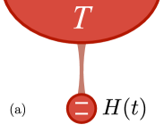
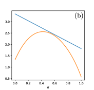
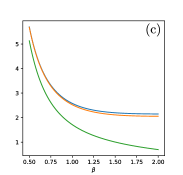
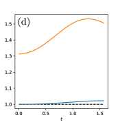
Figure 1: Verification and comparison of our bound in a physical example. (a) The setup considered. A qubit with a time dependant hamiltonian $H(t)$, as given by equation (16) weakly coupled to a bath in temperature $T$. In all simulations the parameters $E=1$, $a=1+i$, $\omega=1$ were used. (b) In this case $\beta=1$ and $t_{f}=\nicefrac{{\pi}}{{2}}$ were used. The graph shows the relative fluctuations $\epsilon_{\alpha}(W)$ (blue curve) compared with our lower bound in equation (5) (orange curve) for different values of $\alpha$ (c) In this case $t_{f}=\nicefrac{{\pi}}{{2}}$, $\beta$ is varied from $0.5$ to 2 and only $\alpha=\nicefrac{{1}}{{2}}$ is considered. The graph shows the relative fluctuations $\epsilon_{\nicefrac{{1}}{{2}}}(W)$ (blue curve), our bound (orange curve) and for comparison the bound in Potts and Samuelsson (2019); Proesmans and Horowitz (2019) (green curve) (d) Time evolution of the fluctuations and the bounds – Here we consider $\beta=1$, $\alpha=\nicefrac{{1}}{{2}}$ and $t_{f}$ varied from 0 to $\nicefrac{{\pi}}{{2}}$. The order of magnitude of fluctuations changes wildly, so we look instead to the ratios of $\epsilon_{\nicefrac{{1}}{{2}}}(W)$ with our bound (blue curve) and with the bound in Potts and Samuelsson (2019); Proesmans and Horowitz (2019) (orange curve). The dashed line at 1 would mark the saturation of the bound.

$$\frac{P_{F}(W)}{P_{B}(-W)}=e^{\beta(W-\Delta F)}$$ (19)

where

$$\Delta F=\frac{1}{\beta}\log\left(\frac{\mathrm{Tr}\left(e^{-\beta H(0)}\right)}{\mathrm{Tr}\left(e^{-\beta H(t_{f})}\right)}\right)\quad\mbox{and}\quad\Sigma=\beta(W-\Delta F)$$ (20)

Since the entropy production in the forwards process is a direct function of the work in the same process and $\Delta F$ changes signs if we switch the forwards and backwards processes, then the equality (19) can indeed be put in the form of equation (2):

$$\frac{P_{F}(\Sigma,W)}{P_{B}(-\Sigma,-W)}=e^{\Sigma}$$ (21)

To find the work distributions for the evolution up to time $t_{f}$, we follow Talkner and Hänggi (2007) and use the characteristic function

$$\chi_{F}(z;t_{f})=\mathrm{Tr}\left(U^{\dagger}e^{izH(t_{f})}Ue^{-izH(0)}\rho_{0}\right)$$ (22)

$$\chi_{B}(z;t_{f})=\mathrm{Tr}\left(Ue^{izH(0)}U^{\dagger}e^{-izH(0)}\rho^{B}_{0}\right)$$ (23)

where $U$ is the unitary operator giving the forwards evolution from the starting state to the final state. Since the drive in (16) is not time symmetrical, then in general we have $U\neq U^{\dagger}$ and $P_{F}\neq P_{B}$. In order to compare with the TUR inequalities in Potts and Samuelsson (2019); Proesmans and Horowitz (2019) we must consider the case $\alpha=\nicefrac{{1}}{{2}}$ in equation (6). Figure 1 contains graphs verifying our bound and comparing it to the one in Potts and Samuelsson (2019); Proesmans and Horowitz (2019) as $\alpha$, $\beta$ and $t_{f}$ are changed. In these graphs it becomes clear the advantage of using higher moments in order to obtain a more precise bound and particularly in figure 1c, our bound is very close to being saturated in the whole range tested.

The role of correlations - An interesting point about our bounds (5) and (7), as well as the earlier bound (4) is that they become trivial in the case $\left\langle\phi\right\rangle_{F}+\left\langle\phi\right\rangle_{B}=0$. However we have

$$\mathrm{Cov}\left(\phi,e^{-\Sigma}\right)_{F}=\left\langle\phi e^{-\Sigma}\right\rangle_{F}-\left\langle\phi\right\rangle_{F}\left\langle e^{-\Sigma}\right\rangle_{F}=-\left(\left\langle\phi\right\rangle_{F}+\left\langle\phi\right\rangle_{B}\right)$$ (24)

That is, the bound in equation (5) can be rewritten as

$$(1-\alpha)\mathrm{Var}\left(\phi\right)_{F}+\alpha\mathrm{Var}\left(\phi\right)_{B}\geq\left(\frac{\alpha^{2}\omega}{\omega-1}-\alpha\right)\mathrm{Cov}\left(\phi,e^{-\Sigma}\right)^{2}_{F}$$ (25)

and hence the bounds trivialize when $\phi$ and $\Sigma$ are uncorrelated. This can be better understood, by checking the solution for $f(\Sigma,\phi)$ in equation (12). The full calculation in the Supplemental Material shows that we must have in this case

$$f(\Sigma,\phi)=\left\langle\phi\right\rangle_{F}$$ (26)

from which one can easily check that $\left\langle f\right\rangle_{F}=\left\langle\phi\right\rangle_{F}$ and $\left\langle-fe^{-\Sigma}\right\rangle_{F}=-\left\langle\phi\right\rangle_{F}=\left\langle\phi\right\rangle_{B}$. In other words, a constant $\phi$ is consistent with our constraints in this case. Note that this is in contrast with the more studied case $P_{F}=P_{B}$ where $\phi$ can only be a constant if the averages are 0. This is a direct consequence of $\left\langle\phi\right\rangle$ being the same in the forwards and backwards process in this case, meaning by equation (24) that there is always a correlation between $\phi$ and $\Sigma$, leading to non-trivial bounds.

Another point relating specifically to the case $\alpha=0$ is that

$$\mathrm{Var}\left(e^{-\Sigma}\right)_{F}=\left\langle e^{-2\Sigma}\right\rangle_{F}-\left\langle e^{\Sigma}\right\rangle_{F}^{2}=\left\langle e^{-2\Sigma}\right\rangle_{F}-1$$ (27)

meaning the inequality for $\alpha=0$ can be rewritten as

$$\mathrm{Var}\left(\phi\right)_{F}\mathrm{Var}\left(e^{-\Sigma}\right)_{F}\geq\mathrm{Cov}\left(\phi,e^{-\Sigma}\right)^{2}_{F}$$ (28)

which follows directly from the positivity of the covariance matrix between $\phi$ and $e^{-\Sigma}$ for the forwards process (by symmetry, the case $\alpha=1$ has the same interpretation, but for the backwards process). Note that even though this makes these cases look trivial, it is still non trivial that the inequality can be saturated.

Conclusions - In this work we have presented a rigorous derivation of a family of thermodynamic uncertainty relations that are direct consequences of fluctuation theorems. Contrary to most similar works, we do not require the forwards and backwards processes to have the same statistics, allowing the application in situations where the Tasaki-Crooks FT holds and situations in the presence of feedback control. The bound is obtained by an optimization procedure and the result can be interpreted as the tightest bound given as constraints the marginal distribution for entropy production and the forwards and backwards averages of the current whose fluctuations we want to bound. We are able to find explicitly which joint distributions saturate the bound, showing that this depends only on what their support is. Finally, we show that our bounds, as well as other bounds known for the case where the forwards and backwards processes are distinct must trivialize when the current is uncorrelated with the entropy production, giving some insight on why this is inevitable. This work therefore furthers significantly the understanding of fluctuations happening in non-equilibrium thermodynamic processes and how they connect with other related results.

I Deduction of the TUR family

Like in the main text, we consider a distribution $P(\Sigma,\phi)$ for the forwards process and want to find the measurable function $f(\Sigma,\phi)$ that minimizes the functional

$$\mathcal{F}[f]=\int P(\Sigma,\phi)f(\Sigma,\phi)^{2}\left(1-\alpha+\alpha e^{-\Sigma}\right)\,\mathrm{d}\phi\,\mathrm{d}\Sigma$$ (S1)

subject to the constraints

$$\int P(\Sigma,\phi)f(\Sigma,\phi)\,\mathrm{d}\phi\,\mathrm{d}\Sigma=\left\langle\phi\right\rangle_{F}$$ (S2)

$$\int P(\Sigma,\phi)f(\Sigma,\phi)e^{-\Sigma}\,\mathrm{d}\phi\,\mathrm{d}\Sigma=-\left\langle\phi\right\rangle_{B}$$ (S3)

In order to do this minimization, we must consider the following Lagrangian functional

$$\mathcal{L}[f]=\int P(\Sigma,\phi)\left(f(\Sigma,\phi)^{2}\left(1-\alpha+\alpha e^{-\Sigma}\right)+\lambda\left(f(\Sigma,\phi)-\left\langle\phi\right\rangle_{F}\right)+\mu\left(f(\Sigma,\phi)e^{-\Sigma}+\left\langle\phi\right\rangle_{B}\right)\right)\,\mathrm{d}\phi\,\mathrm{d}\Sigma$$ (S4)

Since $\mathcal{L}$ is convex whenever $0\leq\alpha\leq 1$ and we have only equality constraints, then for these values of $\alpha$ we can find an equation for the minimum $f$ by simply equating the functional derivative to zero. Since

$$\frac{\delta\mathcal{L}}{\delta f}=P(\Sigma,\phi)\left(2f(\Sigma,\phi)\left(1-\alpha+\alpha e^{-\Sigma}\right)+\lambda+\mu e^{-\Sigma}\right)$$ (S5)

then for all $(\Sigma,\phi)$ in the support we have

$$f(\Sigma,\phi)=\frac{-(\lambda+\mu e^{-\Sigma})}{2\left(1-\alpha+\alpha e^{-\Sigma}\right)}$$ (S6)

The form of the solution is different for $\alpha=0$ and $0<\alpha\leq 1$. We will start with the simplest case:

I.1 The $\alpha=0$ case

In this case eq (S6) can be simplified to

$$f(\Sigma,\phi)=A+Be^{-\Sigma}$$ (S7)

Imposing the constraints leads to the system

$$\left\{\begin{array}[]{l}\left\langle\phi\right\rangle_{F}=\left\langle A+Be^{-\Sigma}\right\rangle_{F}=A+B\vspace{0.2cm}\\ \left\langle\phi\right\rangle_{B}=\left\langle-e^{-\Sigma}\left(A+Be^{-\Sigma}\right)\right\rangle_{F}=-A-B\left\langle e^{-2\Sigma}\right\rangle_{F}\\ \end{array}\right.$$ (S8)

with solution

$$B=\frac{\left\langle\phi\right\rangle_{F}+\left\langle\phi\right\rangle_{B}}{1-\left\langle e^{-2\Sigma}\right\rangle_{F}}\quad\quad\mbox{and}\quad\quad A=\left\langle\phi\right\rangle_{F}-B$$ (S9)

implying that $\left\langle f^{2}\right\rangle_{F}$

rCl ⟨f^2 ⟩_F &= ∫f(Σ, ϕ)^2 P_F(Σ, ϕ)  dΣ dϕ
= ∫(A + B e^-Σ)^2 P_F(Σ, ϕ)  dΣ dϕ
= A^2 + 2AB + B^2 ⟨e^-2Σ ⟩_F
= (A + B)^2 + B^2 (⟨e^-2Σ ⟩_F - 1)
= ⟨ϕ ⟩_F^2 + (⟨ϕ ⟩F+ ⟨ϕ ⟩B)2⟨e-2Σ⟩F- 1 ⇒

$$\mathrm{Var}\left(f\right)_{F}=\left\langle f^{2}\right\rangle_{F}-\left\langle f\right\rangle_{F}^{2}=\frac{(\left\langle\phi\right\rangle_{F}+\left\langle\phi\right\rangle_{B})^{2}}{\left\langle e^{-2\Sigma}\right\rangle_{F}-1}$$ (S10)

Since $\phi$ is a measurable function of $(\Sigma,\phi)$ satisfying the same constraints as $f$, it follows that $\mathrm{Var}\left(\phi\right)_{F}\geq\mathrm{Var}\left(f\right)_{F}$ and hence

$$\mathrm{Var}\left(\phi\right)_{F}\geq\frac{(\left\langle\phi\right\rangle_{F}+\left\langle\phi\right\rangle_{B})^{2}}{\left\langle e^{-2\Sigma}\right\rangle_{F}-1}$$ (S11)

I.2 The $0<\alpha\leq 1$ case

If $\alpha\neq 0$, then eq (S6) can always be rewritten as

$$f(\Sigma,\phi)=A+\frac{B}{\Omega(\Sigma)}\quad\quad\mbox{where}\quad\quad\Omega(\Sigma)=1-\alpha+\alpha e^{-\Sigma}$$ (S12)

Furthermore, if we define

$$\left\langle\frac{1}{\Omega}\right\rangle_{F}=\omega\quad\quad\mbox{and}\quad\quad\left\langle\frac{e^{-\Sigma}}{\Omega}\right\rangle_{F}=\omega^{\prime}$$ (S13)

then we have

$$1=\left\langle\frac{1-\alpha+\alpha e^{-\Sigma}}{\Omega}\right\rangle_{F}=(1-\alpha)\omega+\alpha\omega^{\prime}\quad\Rightarrow\quad\omega^{\prime}=\frac{1-\omega}{\alpha}+\omega$$ (S14)

So imposing the constraints leads to the system

$$\left\{\begin{array}[]{l}\left\langle\phi\right\rangle_{F}=\left\langle A+\nicefrac{{B}}{{\Omega}}\right\rangle_{F}=A+B\omega\vspace{0.2cm}\\ \left\langle\phi\right\rangle_{B}=\left\langle-e^{-\Sigma}\left(A+\nicefrac{{B}}{{\Omega}}\right)\right\rangle_{F}=-A-B\omega^{\prime}\\ \end{array}\right.$$ (S15)

with solution

$$B=\frac{\alpha(\left\langle\phi\right\rangle_{F}+\left\langle\phi\right\rangle_{B})}{\omega-1}\quad\quad\mbox{and}\quad\quad A=\left\langle\phi\right\rangle_{F}-B\omega$$ (S16)

Finally, rCl ⟨f^2Ω ⟩_F &= ⟨(A + BΩ)^2 Ω ⟩_F
= ⟨A^2Ω+ 2AB + B2Ω ⟩_F
= A^2+ 2AB + B^2ω
= (A + B)^2 + B^2(ω- 1)
= (

References

- Benenti et al. (2017) G. Benenti, G. Casati, K. Saito, and R. S. Whitney, Physics Reports 694, 1 (2017).
- Li et al. (2012) N. Li, J. Ren, L. Wang, G. Zhang, P. Hänggi, and B. Li, Rev. Mod. Phys. 84, 1045 (2012).
- Josefsson et al. (2018) M. Josefsson, A. Svilans, A. M. Burke, E. A. Hoffmann, S. Fahlvik, C. Thelander, M. Leijnse, and H. Linke, Nature nanotechnology 13, 920 (2018).
- Dubi and Di Ventra (2011) Y. Dubi and M. Di Ventra, Reviews of Modern Physics 83, 131 (2011).
- Zhang et al. (2023) L. Zhang, Y. Qiu, W.-G. Liu, H. Chen, D. Shen, B. Song, K. Cai, H. Wu, Y. Jiao, Y. Feng, J. S. W. Seale, C. Pezzato, J. Tian, Y. Tan, X.-Y. Chen, Q.-H. Guo, C. L. Stern, D. Philp, R. D. Astumian, W. A. Goddard, and J. F. Stoddart, Nature 613, 280 (2023).
- Kassem et al. (2017) S. Kassem, T. van Leeuwen, A. S. Lubbe, M. R. Wilson, B. L. Feringa, and D. A. Leigh, Chem. Soc. Rev. 46, 2592 (2017).
- Pietzonka and Seifert (2018) P. Pietzonka and U. Seifert, Phys. Rev. Lett. 120, 190602 (2018).
- Barato and Seifert (2015) A. C. Barato and U. Seifert, Physical Review Letters 114, 158101 (2015).
- Pietzonka et al. (2016) P. Pietzonka, A. C. Barato, and U. Seifert, Physical Review E 93, 052145 (2016), arXiv:1512.01221 .
- Pietzonka and Seifert (2017) P. Pietzonka and U. Seifert, Physical Review Letters 120, 190602 (2017), arXiv:1705.05817 .
- Pietzonka et al. (2017) P. Pietzonka, F. Ritort, and U. Seifert, Physical Review E 96, 012101 (2017), arXiv:1702.07699 .
- Gingrich et al. (2016) T. R. Gingrich, J. M. Horowitz, N. Perunov, and J. L. England, Physical Review letters 116, 120601 (2016).
- Dechant (2018) A. Dechant, Journal of Physics A: Mathematical and General 52, 035001 (2018), arXiv:1809.10414 .
- Barato et al. (2018) A. C. Barato, R. Chetrite, A. Faggionato, and D. Gabrielli, New Journal of Physics 20, 103023 (2018).
- Holubec and Ryabov (2018) V. Holubec and A. Ryabov, Physical review letters 121, 120601 (2018).
- Proesmans and Van den Broeck (2017) K. Proesmans and C. Van den Broeck, EPL (Europhysics Letters) 119, 20001 (2017).
- Gallavotti and Cohen (1995) G. Gallavotti and E. G. D. Cohen, Physical Review Letters 74, 2694 (1995).
- Jarzynski (1997) C. Jarzynski, Physical Review E 56, 5018 (1997).
- Crooks (1998) G. E. Crooks, Journal of Statistical Physics 90, 1481 (1998).
- Piechocinska (2000) B. Piechocinska, Physical Review A 61, 062314 (2000).
- Tasaki (2000) H. Tasaki, (2000), arXiv:0009244 [cond-mat] .
- Kurchan (2000) J. Kurchan, (2000), arXiv:0007360 [cond-mat] .
- Jarzynski and Wójcik (2004) C. Jarzynski and D. K. Wójcik, Physical Review Letters 92, 230602 (2004).
- Andrieux et al. (2009) D. Andrieux, P. Gaspard, T. Monnai, and S. Tasaki, New Journal of Physics 11, 043014 (2009).
- Saito and Utsumi (2008) K. Saito and Y. Utsumi, Physical Review B - Condensed Matter and Materials Physics 78, 115429 (2008).
- Esposito et al. (2009) M. Esposito, U. Harbola, and S. Mukamel, Reviews of Modern Physics 81, 1665 (2009).
- Campisi et al. (2011) M. Campisi, P. Hänggi, and P. Talkner, Reviews of Modern Physics 83, 771 (2011).
- Jarzynski (2011) C. Jarzynski, Annual Review of Condensed Matter Physics 2, 329 (2011).
- Talkner and Hänggi (2007) P. Talkner and P. Hänggi, Journal of Physics A: Mathematical and Theoretical 40, F569 (2007).
- Ptaszyński (2018) K. Ptaszyński, Physical Review B 98, 085425 (2018), arXiv:1805.11301v2 .
- MacIeszczak et al. (2018) K. MacIeszczak, K. Brandner, and J. P. Garrahan, Physical Review Letters 121, 130601 (2018), arXiv:arXiv:1803.01904v3 .
- Guarnieri et al. (2019) G. Guarnieri, G. T. Landi, S. R. Clark, and J. Goold, Phys. Rev. Res. 1, 033021 (2019).
- Hasegawa (2023) Y. Hasegawa, Nature Communications 14, 2828 (2023).
- Merhav and Kafri (2010) N. Merhav and Y. Kafri, Journal of Statistical Mechanics: Theory and Experiment 2010 (2010), 10.1088/1742-5468/2010/12/P12022.
- Hasegawa and Van Vu (2019) Y. Hasegawa and T. Van Vu, Phys. Rev. Lett. 123, 110602 (2019).
- Potts and Samuelsson (2019) P. P. Potts and P. Samuelsson, Phys. Rev. E 100, 052137 (2019).
- Timpanaro et al. (2019) A. M. Timpanaro, G. Guarnieri, J. Goold, and G. T. Landi, Phys. Rev. Lett. 123, 090604 (2019).
- Ray et al. (2023) K. J. Ray, A. B. Boyd, G. Guarnieri, and J. P. Crutchfield, Phys. Rev. E 108, 054126 (2023).
- Sagawa and Ueda (2012) T. Sagawa and M. Ueda, Phys. Rev. E 85, 021104 (2012).
- Proesmans and Horowitz (2019) K. Proesmans and J. M. Horowitz, Journal of Statistical Mechanics: Theory and Experiment 2019, 054005 (2019).
Supplemental Material