Boost Your NeRF: A Model-Agnostic Mixture of Experts Framework for High Quality and Efficient Rendering

Abstract

Since the introduction of NeRFs, considerable attention has been focused on improving their training and inference times, leading to the development of Fast-NeRFs models. Despite demonstrating impressive rendering speed and quality, the rapid convergence of such models poses challenges for further improving reconstruction quality. Common strategies to improve rendering quality involves augmenting model parameters or increasing the number of sampled points. However, these computationally intensive approaches encounter limitations in achieving significant quality enhancements. This study introduces a model-agnostic framework inspired by Sparsely-Gated Mixture of Experts to enhance rendering quality without escalating computational complexity. Our approach enables specialization in rendering different scene components by employing a mixture of experts with varying resolutions. We present a novel gate formulation designed to maximize expert capabilities and propose a resolution-based routing technique to effectively induce sparsity and decompose scenes. Our work significantly improves reconstruction quality while maintaining competitive performance.

1 Introduction

Neural Radiance Fields (NeRFs) [25] have recently shown impressive results in synthesizing photo-realistic 3D scenes from a set of 2D images. However, NeRFs suffer from limited scene diversity, long training time, and sensitivity to training data [22]. Since the introduction of NeRFs, significant attention has been directed toward improving their training and inference times, resulting in the development of Fast-NeRFs. By using auxiliary data structures such as voxel grids to store scene geometry and skip empty spaces, the training and inference process can be accelerated by several orders of magnitude. As a result, the neural component of these models, which is usually used to transform learned features into view-dependent color representations, becomes much smaller and can sometimes be replaced entirely by spherical harmonics [11]. Despite Fast NeRFs being an improvement from the original NeRF framework, achieving high-quality and efficient reconstructed geometry is still an open problem.

Typical “naive” approaches to enhance the reconstruction quality of these models include:

1. Increasing the parameters and resolution of the used data structures (e.g., voxel grid, hash grid, etc.).

2. Increasing the number of sampled points per ray.

3. Increasing the number of parameters in the neural network or the order of spherical harmonics.

However, as evident from Figure 1, the increase in reconstruction quality results in a significant increase in computational costs. In the first approach, increasing the resolution can lead to a significant improvement in the reconstruction quality, but a plateau is reached beyond which overfitting occurs, and reconstruction quality degrades. This comes at the expense of a considerable increase in spatial complexity (especially with dense voxel grids) and training times. Increasing the number of sampled points per ray can marginally improve reconstruction quality further but at a significant increase in computational complexity. In fact, the higher the number of sampled rays, the higher forward passes through a neural network are needed. Augmenting the number of parameters in the neural network is another solution. However, as the neural network grows in depth and width, it tends towards a fully implicit model, deviating from the principles of fast models (limiting the neural part as much as possible - or even removing it altogether).

Figure 1: Different strategies for improving reconstruction quality with Fast-NeRFs (DVGO [30]). Increasing the resolution of data structures like voxel grids can improve render quality, but only up to a certain point, after which quality declines (left). The MLP component’s impact on rendering quality is analyzed by varying its depth and width while keeping other variables constant (center). The effect of the number of sampled points along each ray is examined by decreasing the step size (right). In gray, our method’s performance, which significantly improves PSNR at a low computational cost.

We propose a technique capable of significantly enhancing the reconstruction quality of such models while maintaining competitive training and rendering times. Inspired by the Sparse Mixture of Experts (MoE) paradigm [29], we have developed a model-agnostic framework capable of improving the reconstruction quality of various state-of-the-art models. Intuitively, our mixture of experts consists of different-capacity (resolution) models. During training, each model specializes in rendering the most suitable parts of the scene, i.e. low-resolution models render low-frequency parts of the scene, while high-resolution models render high-frequency parts. Our formulation of the gate allows our method to be model-agnostic, enabling, on the one hand, the insertion of the gate function at the early stages of the MoE mechanism and, on the other hand, the multiplication of the gate’s output with the experts’ output as late as possible. This maximizes the capabilities of the mixture of experts and allows for working directly with the output of each expert, which is considered a black box. This is why our method is inherently model-agnostic. In summary, our contributions are as follows:

1. We propose the first model-agnostic framework based on Sparse MoE of models at different resolutions, which significantly improves the rendering quality of such models while maintaining competitive training and inference times (Sec. 3).

2. We provide a novel gate formulation inspired by Fast-NeRF models, which maximizes the capability of the mixture of experts (Sec. 3.3).

3. We introduce a new routing technique based on resolution, favoring the assignment of tokens to low-resolution models and discouraging the assignment of tokens to high-resolution models, inducing increasing sparsity in high-resolution models and decomposing the scene based on frequency (Sec. 3.5).

4. We conduct extensive experiments to test our method, including different NeRFs architectures and datasets, showing higher rendering quality and efficiency (Sec. 4).

2 Related works

2.1 Neural Radiance Field

NeRF [25] (Neural Radiance Field) has emerged as a prominent method for synthesizing novel views, showing significant progress. This approach requires a moderate number of input images along with their known camera poses. Unlike traditional methods that rely on explicit and discretized volumetric representations such as voxel grids and multiplane images, NeRF employs a coordinate-based multilayer perceptron (MLP) to create an implicit and continuous volumetric representation. NeRFs can represent a 3D scene as a MLP $F_{\theta}$, with $\theta$ being the set of its trainable parameters, such that $F_{\theta}:(\mathbf{x},\mathbf{d})\rightarrow(\mathbf{c},\sigma)$ which maps $(\mathbf{x},\mathbf{d})$, a 3D position $\mathbf{x}$ and a viewing direction $\mathbf{d}$, to a view-dependent color emission $\mathbf{c}$ and density value $\sigma$. To render the color of a pixel $\hat{C}(\mathbf{r})$, a ray $\mathbf{r}$ traverses the center of the camera through the pixel of the image plane from an origin point $\mathbf{o}$ to a ray having position $\mathbf{r}(t)=\mathbf{o}+t\mathbf{d}$. Then, $N$ points are sampled on $\mathbf{r}$, and the MLP is queried for each point, obtaining a density and a color value. Finally, these results are accumulated into a single color with the volume rendering equation [23]:

$$\hat{{C}}(\mathbf{r})=\sum_{i=1}^{K}T_{i}\alpha_{i}c_{i},\qquad T_{i}=\prod_{j=1}^{i-1}(1-\alpha_{j}),\qquad\alpha_{i}=1-\exp(\sigma_{i}\delta_{i}),$$ (1)

where $\alpha_{i}$ is the probability of termination at point $i$ and $T_{i}$ is the accumulated transmittance from the near plane to point $i$. NeRFs are trained by minimizing a photometric loss, which is an L2 loss between the rendered and the ground truth pixels. In more detail, given a batch $B$ of randomly sampled rays, the loss is defined as

$$L_{\text{nerf}}=\frac{1}{|B|}\sum_{r\in B}\left\|\hat{C}(\mathbf{r})-C(\mathbf{r})\right\|^{2}_{2},$$ (2)

where $\hat{C}(\mathbf{r})$ is the predicted color and $C(\mathbf{r})$ the ground truth color for the ray $\mathbf{r}$.

2.2 Fast Neural Radiance Fields

Since the introduction of NeRF, significant effort has been directed towards the development of faster models. Several studies focus on speeding up rendering times, for example by working on ray sampling efficiency [4, 7, 13, 38], by integrating explicit volumetric representations [12, 16, 32, 34, 33, 12, 6] or by utilizing thousands of tiny MLPs [27]. However, all these methods still require large training times. One noteworthy development is represented by the introduction of explicit volumetric representations in the training pipeline, directly optimizing such representations [11, 30, 5, 26, 10, 14, 17]. These models enable fast training and inference, with render quality only slightly inferior to full-implicit models [1, 3]. We refer to these as Fast-NeRFs. Plenoxels [11] is the first important work in this context, as it represents a scene as a sparse 3D grid where each voxel stores spherical harmonic coefficients and density. Spherical harmonics serve as an orthogonal basis for functions defined over the sphere and thus can be used for computing view-dependent color emission, without the need for a multi-layer perceptron. Additionally, Plenoxels demonstrated the advantages of linearly interpolating voxels, facilitating the learning of a continuous plenoptic function throughout the volume, akin to NeRF, albeit with discrete data. Another notable work is DVGO [30]. Each scene is there represented as two dense voxel grids (one for density and one for feature colors) alongside a MLP, for learning view-dependent color. Similar to Plenoxels, the value of each voxel is linearly interpolated with the 8 nearest voxels, but after applying the activation functions. DVGO also incorporates a preliminary coarse geometry stage to learn the scene’s general structure, facilitating adjustments to the bounding box and enabling a more intelligent ray sampling strategy. Despite utilizing lower-resolution models, DVGO achieves high reconstruction quality. The major drawback of these models is their substantial memory storage requirements. TensoRF [5] addresses this challenge by replacing the dense voxel grid with a planes and vectors decomposition, significantly reducing storage demands while maintaining comparable performance and rendering quality. Alternatively, Instant-NGP [26] proposed a multi-resolution voxel grid encoded via a hash function. They define $L$ hash grids of increased resolutions: each entry of each hash grid has $2^{T}$ parameters and $F$ features. This enables even faster training times and real-time rendering performances while maintaining a compact model; moreover, it demonstrates the efficacy of a multi-resolution approach in enhancing render quality. Inspired by this methodology, K-Planes [10] introduces a multi-resolution planar factorization of 3D space, offering reconstruction quality and model compactness similar to the previous methods, but with slightly larger training times. A similar multi-resolution planar factorization has also been proposed in Tri-MipRF [14] for mitigating the aliasing in distant or low-resolution views and blurriness in close-up shots. Given their properties, we decided to evaluate our paradigm using three different models: a 3D dense voxel grid-based model (DVGO), a decomposed grid-based model (TensoRF), and a multi-resolution hash grid-based model (Instant-NGP).

2.3 Mixture of Experts and Sparse MoE

The Mixture of Experts (MoE) paradigm [15] has gained prominence in various machine learning applications. MoE consists of multiple expert networks, each specializing in different regions of the input space, with a meta-network determining the contribution of each expert to the final prediction. Building upon the MoE framework, Sparse Mixture of Experts [29, 20, 28, 37] constitutes a scalable and efficient variant. At the core of all Sparse MoE algorithms lies an assignment problem between tokens and experts. One approach to tackle this is by approximating the solution with a gating function, which learns to assign input tokens to the most suitable experts. It typically comprises a linear layer, a softmax activation, and a Top-$K$ (where $1\leq K\leq 2$) operation, aimed at routing the input token to only a subset of the experts. To balance the assignment across all the experts, auxiliary loss functions penalizing unevenly distributed routing are often employed. This sparsity-inducing technique significantly reduces computational overhead while preserving the expressive power of the MoE architecture.

2.4 MoE and NeRF

Combining the sparse mixture of experts’ paradigms with neural radiance fields presents a non-trivial challenge. In recent research, Switch-NeRF [36] has been introduced as a novel end-to-end large-scale NeRF with learning-based scene decomposition. Inspired by Fedus et al. [9], they propose a full-implicit model with an MLP-based gate comprising 4 layers with 128 neurons and a Top-$1$ function. However, their architecture is ad-hoc, and suffers from extensive training times. This poses a challenge for us, as we aim to consider each expert as a black box, taking a point in space and a direction as input and outputting radiance and density values. Moreover, as the mixture comprises experts at different resolutions, we also aim to prioritize routing input tokens toward lower-resolution models and minimize the usage of high-resolution models.

Our work intends to overcome these limitations. We design a novel gate formulation inspired by Fast-NeRFs, that guarantees fast convergence and better performances. We position the gate at the beginning of our MoE pipeline and postpone the multiplication of the gate output with expert predictions as much as possible. This allows our framework to be entirely model-agnostic. Furthermore, our mixture of experts maintains competitive training times, enabling, in the worst case, training models on complex scenes in approximately 1 hour while achieving state-of-the-art accuracy.

3 Method

In this section, we introduce our model-agnostic ensembling approach. We present in Sec. 3.1 an overview of our method. We also describe the ray sampling and filtering mechanism in Sec. 3.2. Then, in Sec. 3.3, we discuss the effective construction of a mixture of experts with a gating mechanism in the context of NeRF. Finally, in Sec. 3.5, we present a novel formulation for decomposing the scene into resolution-based parts with an end-to-end training procedure.

3.1 Overview

Figure 2: A density field is used to compute density values for sampled points along a ray. A filtering step discards low-density points, routed through gating network $G$ for expert assignment. Top-$K$ experts compute radiance and density, aggregating and weighting these values by the corresponding gating probability to get the final values $\mathbf{c}_{f}$ and $\sigma_{f}$. Volume rendering equation yields pixel colors, and joint optimization refines our resolution-weighted auxiliary loss, allowing for high-quality and efficient rendering.

Figure 2 shows a high-level scheme of our method. After independently training a set of $M$ NeRF models $\{E_{i}\}_{i=1}^{M}$ at different resolutions, we sample $N$ points along a ray $\mathbf{r}$. For each point $\mathbf{x}_{p}$, a density value $\sigma$ is calculated, and based on this, a filtering step is performed based on the density volume $\mathbf{V}_{D}$, discarding points in regions with a density below a certain threshold $T$. Initializing the density volume $\mathbf{V}_{D}$ with the one learned from the lowest resolution model can be helpful (though it can also be learned). Subsequently, the filtered point $\mathbf{x}_{f}$ is fed to the gate $G$, so we denote with $G(\mathbf{x}_{f})$ the probabilities with which the point is assigned to the $M$ experts. Based on these values, each point is routed to the Top-$K$ experts. Each selected expert then computes the radiance $\mathbf{c}_{i,f}$ and density values $\sigma_{i,f}$ for the point, both of which are multiplied by their respective probabilities and summed together to get the final radiance $\mathbf{c}_{f}$ and density $\sigma_{f}$. Subsequently, the volume rendering Equation 1 is used to aggregate all colors and compute the pixel color for the given ray. Finally, we compute the total loss and jointly optimize the gate and the experts.

In the next sections, we will dive into the gating and sparse mixture of expert modules.

3.2 Ray sampling and filtering

The first phase of our method involves learning a coarse and explicit density field starting from the density volume $\mathbf{V}_{D}$, that we can leverage for skipping empty spaces. Given a ray $\mathbf{r}$ as explained in Sec. 2.1, we sample $N$ points along it:

$$\mathbf{X}_{p,r}=\operatorname{sampling}(\mathbf{r})\in\mathbb{R}^{N\times 3},$$ (3)

with $p\in[0,...,N-1]$. We suppress the index $r$ for abuse of notation. Next, we compute the density for each point $\mathbf{x}_{p}\in\mathbb{R}^{3}$ and discard those with negligible density. The density value $\mathbf{\sigma}_{D,p}$ for each point is computed by linearly interpolating $v$ neighboring voxels:

$$\sigma_{D,p}=\operatorname{act}(\operatorname{interpolate}(\mathbf{x}_{p},V_{D}))\in\mathbb{R}$$ (4)

where $\operatorname{act}$ represents a density activation function (such as softplus). We denote with $\mathbf{x_{f}\in\mathbb{missing}}{R}^{3}$ a remaining point after the filtering operation.

3.3 Trainable Gating Model

Our gating mechanism incorporates a hybrid architecture: an explicit feature grid $\mathbf{V}_{G}$ and a shallow MLP. The gating mechanism can also be seen as a probability field. First, we compute per-point features:

$$\mathbf{feat}=\operatorname{interpolate}(\mathbf{x}_{f},\mathbf{V}_{G})\in\mathbb{R}^{C}$$ (5)

where $C$ represents the number of channels of $\mathbf{V}_{G}$. Subsequently, we transform each feature into a probability. We compute logits as

$$\mathbf{logits}=\operatorname{MLP}(\mathbf{feat})\in\mathbb{R}^{M}$$ (6)

where $M$ is the number of experts in the mixture of experts. Finally, we apply a per-row softmax. Our gating function can be summarized as:

$$G(\mathbf{\mathbf{x}_{f}})=\operatorname{softmax}(\operatorname{MLP}(\operatorname{interpolate}(\mathbf{x}_{f},\mathbf{V}_{G})))\in\mathbb{R}^{M}$$ (7)

3.4 NeRFs Experts

As mentioned in Sec. 3.1, we employ a set of $M$ pretrained NeRFs models as experts. After feeding as input each point $\mathbf{x}_{f}$ to the gate, we route them to the $k$ experts with the $k$ highest probabilities $G(\mathbf{x}_{f})$. We define this set of indexes of the selected experts as

$$\mathcal{K}=\operatorname*{argmax}_{Top-k}(G(\mathbf{x}_{f})).$$ (8)

Each expert is a Fast-NeRF model that receives the dispatched points and the direction of the ray they lie on as input and outputs a density and a radiance value. We treat each expert as a black box, ensuring our method is inherently model-agnostic. The radiance $\mathbf{c}_{f}$ and the density $\sigma_{f}$ for the point $\mathbf{x}_{f}$ laying on a ray with direction $\mathbf{d}$ can be expressed as the sum of each expert predictions weighted by their probability:

$$\mathbf{c}_{f},\sigma_{f}=\sum_{i\in\mathcal{K}}E_{i}(\mathbf{x_{f}},\mathbf{d})\cdot G(\mathbf{x_{f}})_{i}$$ (9)

where $E_{i}$ denotes the $i$-th expert and $G(\mathbf{x_{f}})_{i}$ the probability for the point to be dispatched to that expert $i$.

Once we obtain radiance and density values for all the points on the ray, we can compute the pixel color with Equation 1.

3.5 Resolution-based routing

To balance the load and prevent the gate from focusing on assigning points to a single expert (typically the one with the highest resolution), we employ a resolution-weighted auxiliary loss. Given $M$ experts, and a batch of points $B$, the auxiliary loss is defined as:

$$L_{\text{aux}}=\frac{M}{|B|^{2}}\sum_{i=1}^{M}c_{i}m_{i},\qquad m_{i}=\sum_{\mathbf{x}_{f}\in B}G(\mathbf{x}_{f})_{i},$$ (10)

where $c_{i}$ represents the number of inputs dispatched to the expert $i$, and $m_{i}$ is the sum of all the probabilities for each point in the batch for the expert $i$. This loss helps balance the workload, ensuring that each expert processes a similar number of points. Ideally, in a perfectly balanced scenario, $L_{aux}$ is expected to be 1, as both $c_{i}$ and $m_{i}$ would be $\frac{M}{N}$, resulting in $\sum_{i=1}^{M}c_{i}m_{i}$ being $\frac{M^{2}}{N}$. However, in the case of total imbalance, it tends to the number $M$. We aim to take a step further by assigning as many points as possible to low-resolution experts while discouraging point assignment to high-resolution models. Hence, we introduce some penalty terms $w_{i}$ associated with each expert. The higher the resolution of the model, the higher the penalty. We define a novel resolution-based auxiliary loss:

$$L_{\text{rw-aux}}=\frac{M}{|B|^{2}}\sum_{i=1}^{M}c_{i}m_{i}w_{i}.\qquad$$ (11)

As for the weighting strategy, we opted for the following geometric progression. The weight $w_{i}$ for the $i$ expert is computed as:

$$w_{i}=\exp\left(\frac{\ln M}{M-1}\right)^{i},\quad i\in[0,...,M-1].$$ (12)

The total loss is then defined as:

$$L_{\text{tot}}=L_{\text{nerf}}+\lambda L_{\text{rw-aux}}.$$ (13)

As we will see in Sec. 4, our proposed loss not only further improves the reconstruction quality but also encourages sparsity in higher-resolution models. A comparison with other weighting strategies is proposed in the Supplementary 9.

4 Experiments

4.1 Setting

The code was written in Python 3.8, using PyTorch 1.12, and executed on a single NVIDIA A40 GPU. We tested our technique on the DVGO, TensoRF, and Instant-NGP architecture. The code from official repositories was used as the starting point. For Instant-NGP, the native implementation in PyTorch ngp_pl was employed, which exhibits comparable performance and reconstruction quality to the official NVIDIA implementation. We experimented with various configurations, ranging from a minimum of 3 models to 5 models of different resolutions. The experts are ordered by resolution, such that the $i+1$-th expert has approximately double the parameters of the $i$-th expert. For all configurations and models, $\lambda$ was set to $10^{-3}$. The Gate consists of a grid (dense voxel grid for DVGO, factorized grid for TensoRF, and hash grid for Instant-NGP) and a shallow MLP (2 layers with 64 neurons each) with ReLU activation function. The resolution of the gate is low: $128^{3}$ for both DVGO and TensoRF, while for Instant-NGP we used $L=6$. The number of iterations is set to $20k$ for all the architectures. All other hyperparameters are left as the original implementations. We draw experiments with our method using Top-$k$ experts, with $k=1$ and $k=2$. We compare our results versus baselines with comparable resolutions, as well as a Fast-NeRF ensemble (Ens) obtained by jointly fine-tuning all models and averaging their predictions. It can be noted that this ensemble can be interpreted as a limit case for our method with $k=M$ and $G(\mathbf{x}_{f})_{i}=1/M,\forall i$ similar to the method proposed by [8].

Table 1: Results on DVGO, TensoRF and Instant-NGP with $M=5$. $\|w\|_{0}$ is expressed as multiple of $10^{6}$, while for Instant-NGP as a multiple of $10^{5}$.

Dataset	Metrics	DVGO				TensoRF				Instant-NGP
		baseline	Top-1	Top-2	Ens	baseline	Top-1	Top-2	Ens	baseline	Top-1	Top-2	Ens
Blender	$\mathbf{PSNR}\uparrow$	33.04	33.43	33.74	33.79	32.98	33.68	34.09	34.00	33.35	33.56	33.83	34.01
	$\mathbf{SSIM}\uparrow$	0.961	0.964	0.965	0.966	0.958	0.965	0.968	0.968	0.963	0.963	0.965	0.966
	$\mathbf{LPIPS}\downarrow$	0.026	0.024	0.022	0.022	0.029	0.023	0.021	0.022	0.025	0.045	0.043	0.042
	$\|w\|_{0}\downarrow$	99	26	39	97	40	24	33	49	31	17	21	26
	$\mathbf{GFLOPs}\downarrow$	635	499	940	2206	886	732	1344	2214	46	71	123	208
	$\mathbf{Time}\downarrow$	26’	21’	25’	32’	44’	69’	76’	70’	11’	32’	34’	37’
NSVF	$\mathbf{PSNR}\uparrow$	35.21	37.12	37.59	37.68	36.70	37.40	37.98	38.08	36.44	33.59	37.04	37.31
	$\mathbf{SSIM}\uparrow$	0.977	0.984	0.986	0.986	0.981	0.984	0.986	0.987	0.983	0.983	0.984	0.985
	$\mathbf{LPIPS}\downarrow$	0.015	0.009	0.008	0.007	0.013	0.009	0.008	0.008	0.010	0.023	0.022	0.020
	$\|w\|_{0}\downarrow$	95	27	43	100	42	28	38	54	30	17	20	27
	$\mathbf{GFLOPs}\downarrow$	564	430	811	1903	706	575	1053	1763	28	52	72	123
	$\mathbf{Time}\downarrow$	12’	22’	25’	30’	46’	75’	75’	75’	10’	31’	33’	34’
TaT	$\mathbf{PSNR}\uparrow$	28.93	29.14	29.27	29.37	28.44	28.78	29.14	29.11	29.07	29.16	29.32	29.38
	$\mathbf{SSIM}\uparrow$	0.927	0.925	0.929	0.932	0.905	0.924	0.929	0.928	0.924	0.927	0.929	0.930
	$\mathbf{LPIPS}\downarrow$	0.107	0.108	0.105	0.103	0	0.106	0.099	0.109	0.101	0.125	0.124	0.121
	$\|w\|_{0}\downarrow$	74	16	26	65	7	9	15	80	88	37	47	70
	$\mathbf{GFLOPs}\downarrow$	2666	1626	3066	7198	3567	2791	5126	9146	211	229	531	1003
	$\mathbf{Time}\downarrow$	22’	25’	28’	38’	72’	70’	78’	101’	14’	37’	39’	45’
LLFF	$\mathbf{PSNR}\uparrow$	26.24	26.43	26.62	26.65	26.71	26.73	27.09	27.10	24.97	24.90	25.17	25.19
	$\mathbf{SSIM}\uparrow$	0.831	0.832	0.839	0.843	0.835	0.836	0.862	0.864	0.764	0.763	0.777	0.778
	$\mathbf{LPIPS}\downarrow$	0.136	0.115	0.111	0.107	0.114	0.111	0.101	0.101	0.128	0.239	0.237	0.234
	$\|w\|_{0}\downarrow$	62	26	40	113	19	11	16	23	152	68	75	148
	$\mathbf{GFLOPs}\downarrow$	1678	1514	2508	4972	4542	3226	5921	13522	573	887	1391	2712
	$\mathbf{Time}\downarrow$	24’	28’	32’	36’	58’	49’	57’	68’	24’	25’	46’	42’

4.2 Metrics and Datasets

For each test, image-quality metrics such as PSNR, SSIM [31], and LPIPS [35] (computed on AlexNet [19]) are presented. Additionally, we report the number of non-zero parameters as $\|w_{0}\|$, the average GFLOPs required by each model to render the images of the test set, and total training times. We present results obtained across four major datasets, namely: Synthetic-NeRF [25], Neural Sparse Voxel Field Dataset (NSVF) [21], TanksAndTemple [18], and Local Light Field Fusion Dataset (LLFF) [24].

4.3 Quantitative results

The main experimental results in terms of the metrics defined above are shown in Table 1. Here, we present the results obtained using a mixture of $M=5$ experts; further configurations can be found in the supplementary Sec. 12. Our experiments reveal that our MoE provides a significant rendering quality improvement with respect to the baseline with no or limited impact in terms of computational cost. The increase in rendering quality is notable in Synthetic NeRF (up to 1 dB) and NSVF (up to 1.3 dB). Although more moderate, improvements are still evident, even in more challenging datasets such as TanksAndTemple and LLFF, with about 0.5 dB gain. While Top-$1$ can already achieve state-of-the-art render quality, the Top-$2$ strategy further enhances image quality, reaching levels comparable to the ensemble but with much greater efficiency (about half the average FLOPs per rendering) and using significantly fewer parameters. This observation is also illustrated in Figure 3 , where FLOPS/PSNR plots are shown (each marker in every curve refers to the cases with $M=3,4,5$ experts respectively). Training times are on average are longer but still acceptable (in the worst-case scenario, around 1h is required to train our MoE). However, in the case of Top-1, they can be faster than baselines. This is because of our resolution methods, which tend to favor low-resolution models. Based on these analyses, the Top-$2$ strategy strikes an excellent quality/cost trade-off. The ensembling configuration, using all experts, represents an upper bound in terms of image quality while being the worst case in computational terms.

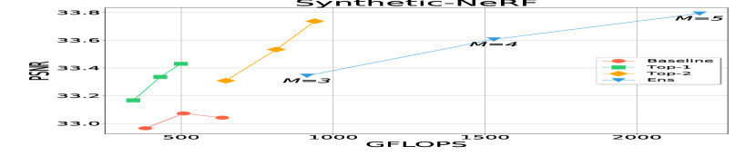
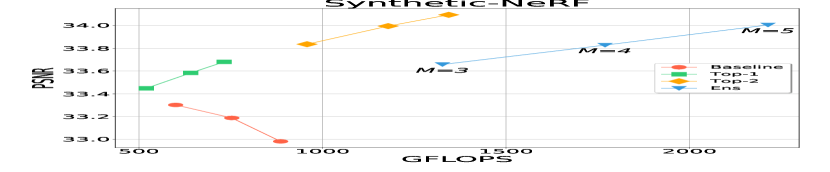
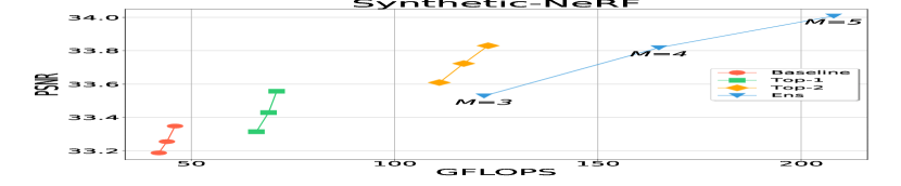
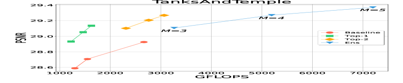
(a) DVGO

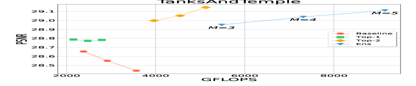
(b) TensoRF

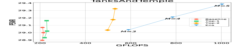
(c) Instant-NGP

Figure 3: PSNR/GFLOPs plots for Synthetic-NeRF and TanksAndTemple. The remaining datasets show similar results.

4.4 Qualitative results

Figure 4 shows visual comparisons among the baseline, ensemble, Top-$1$, and Top-$2$.

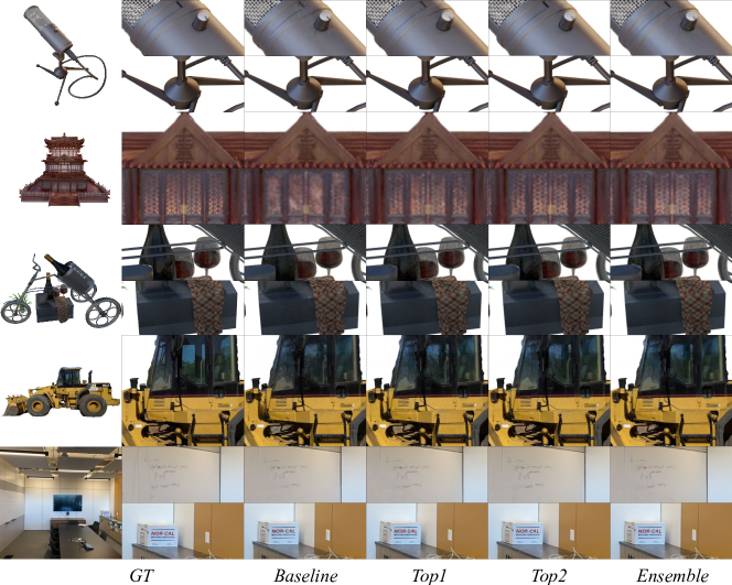
Figure 4: Qualitative results on some of the scenes of each dataset. From left to right: ground truths, baselines, Top-1, Top-2 and Ensemble. Each model has the same parameters and has been trained for the same number of iterations (DVGO).

From the selected image crops, one can appreciate that our method ensures superior reconstruction quality compared to the baselines, effectively reproducing sharper details while reducing noise on texture-less spots. This is particularly notable when examining elements such as the window decorations in the Palace scene or the text on the box above the desk in the Room scene. Additionally, surfaces such as the semi-transparent glass in the Wineholder or the Caterpillar scene appear less noisy and more faithful to the original. This improvement can be attributed to the synergy among different resolution models: low-resolution models excel at representing lower frequencies, thereby introducing less noise, while high-resolution models can focus solely on high-frequency components. Additionally, it is important to notice that there is no significant difference between the ensemble and Top-$2$.

4.5 Comparison with naive methods

As shown in Figure 1, our method leads to significantly higher quality reconstructions at a greatly reduced computational cost. Decreasing the step size yields the least noticeable improvement while incurring a substantial computational expense, as each sampled point requires an evaluation by the color decoder. Our method achieves high-quality reconstructions with the same step size as the baseline models. Increasing the MLP parameters can boost accuracy, but again, the computational costs become substantial compared to our method. Similarly, increasing resolution results in way inferior PSNR with respect to our method at a comparable computational cost. Our method also allows scaling to higher resolutions, while baseline models tend to introduce noise and artifacts, leading to a decrease in reconstruction quality as the resolution increases.

4.6 Gate Visualization and Scene Decomposition

In Figure 5, we visualize the gate (probability field in grayscale) and each expert output in the case $M=3$. On the right side of the figure, one can appreciate per-model renders and experts’ specialization. It is worth noting how higher-resolution experts render high-frequency details. This is particularly evident in the Mic scene.

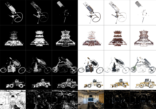
Figure 5: Gate (gray-scale images) and per-model output visualizations with 3 experts and resolution-based routing (DVGO). Images are ordered by increasing resolutions.

4.7 Ablation

Res	Gate Type	$\mathbf{PSNR}$	$\|w\|_{0}$	$\mathbf{GFLOPs}$
$128^{3}$	Ours	36.8	26	476
$256^{3}$	Ours	36.77	33	601
$300^{3}$	Ours	36.79	42	677
-	Linear	36.25	24	444
-	Switch-NeRF	36.44	25	1095

Table 2: Comparison of different gate resolutions and formulations on Lego scene and DVGO.

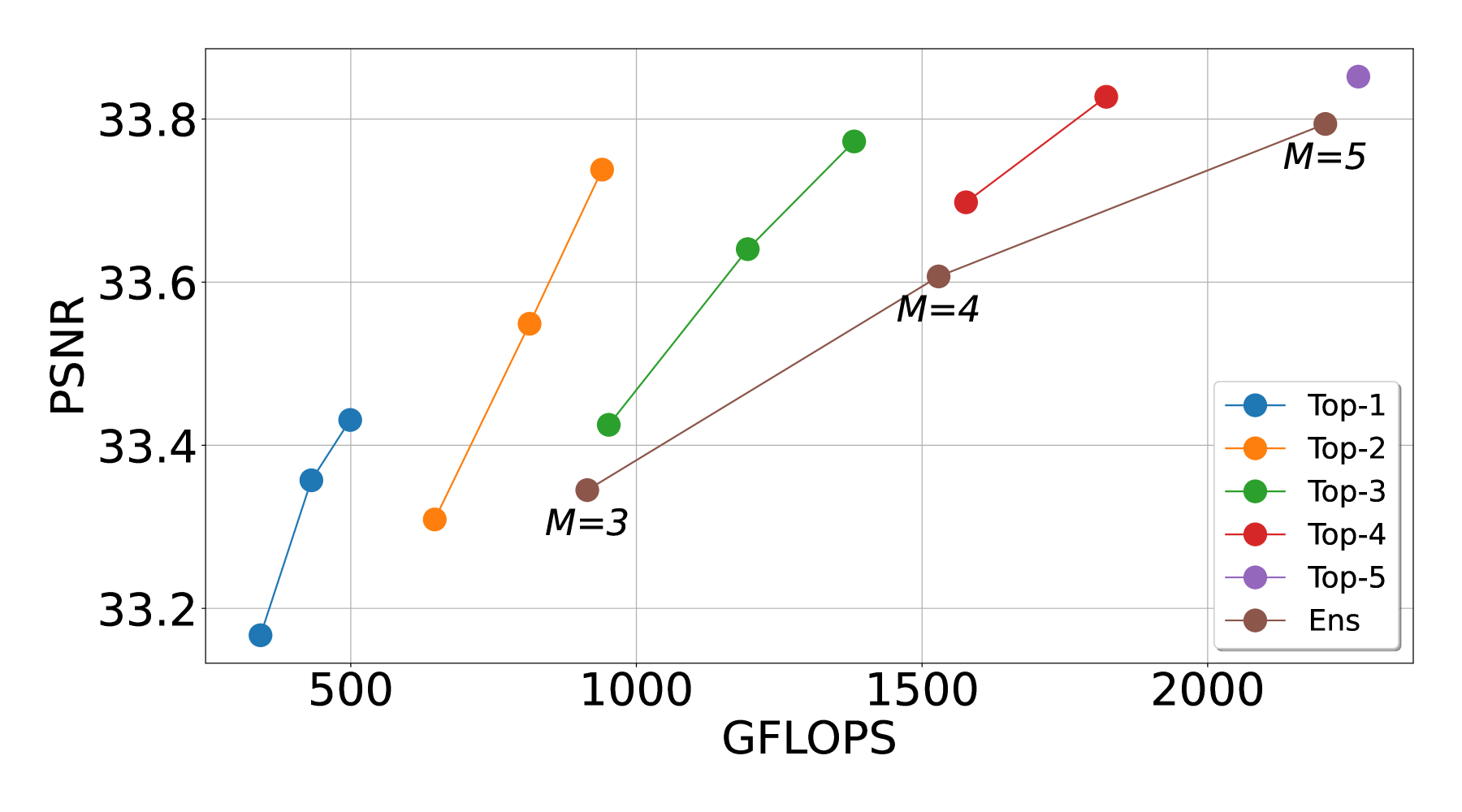
Figure 6: Comparison of Gating Functions (Top-1 to Top-5) on Synthetic-NeRF with DVGO.

Here we investigate how different design choices of our model affect the performance and rendering quality. These choices include the gate resolution, different gate formulations, and the number of experts in the Top-$k$.

Here we investigate how different design choices of our model affect the performance and rendering quality. These choices include the gate resolution, different gate formulations, and the number of experts in the Top-$k$.

4.7.1 Gate Resolution and Gate Formulation.

We show in Table 2 that a low-resolution gate is sufficient to achieve high-quality rendering. Interestingly, as the gate resolution increases, there is a slight decrease in rendering quality during testing, coupled with an increase in required FLOPs per image rendering and number of parameters. We also compare various gating strategies, including linear gating, the configuration proposed by Switch-NeRF, and our gate formulation. Through experimentation, it becomes evident that our approach outperforms others in terms of both render quality and performance, achieving performances comparable to a linear gating function.

4.7.2 Why Top-2?

Here we investigate the performance and rendering quality trends with varying values of $k$. In Figure 6, we can see that while $k=1$ can lead to a significant increase in quality with comparable performance to baseline models, the Top-2 further enhances quality at the expense of increased (but still acceptable) computation. The Top-3, Top-4, and Top-5 provide marginal quality improvements at a significantly higher computational cost. Hence, we consider the Top-2 the optimal balance between performance and quality.

5 Limitations

Our study present some limitations. First of all, a pre-training phase, on which each model is trained independently is required for achieving good results. Training end-to-end, without a pre-training phase, can lead to reconstruction quality that is noticeably inferior to baselines. Pre-training models at different resolutions allows for diversified architectures, making it easier for the gate to learn the decomposition. The training is also strongly dependent on the auxiliary loss. Different values of $\lambda$ can significantly influence performances and load balancing. We conducted a sweep to identify a value that works well across many scenarios, but it may not be suitable for different datasets. Another limitation is the overhead introduced by the MoE. Each input token is first interpolated with the gate’s grid, decoded into probabilities and routed to the chosen expert. These operations can significantly slow-down the rendering process, leading to higher training and inference times. Although considerable effort was devoted to developing the most efficient gate possible, our MoE is still slower than the respective baselines.

6 Conclusions

In this paper, we introduced a model-agnostic framework for enhancing the rendering of Fast-NeRF models. Our formulation of the Gate reduces computational costs in both training and inference phases while ensuring better quality compared to a traditional gate. Additionally, the introduction of an auxiliary loss with res penalty allows for increased utilization of low-resolution models, reducing the number of active parameters and promoting sparsity in higher-resolution models. Our results demonstrate how this approach can significantly improve reconstruction quality while considering performance metrics. Specifically, we show that a Top-2 strategy strikes a good balance between performance and quality.

7 Additional Details

Our MoE is reducible to a Sparsely-Gated Mixture of Experts with full capacity. Since the number of points sampled is reasonable, we did not find necessary to impose a limit to the capacity factor of each model. We also introduce different-resolution experts in the MoE, promoting the routing of tokens towards lower-resolution experts. Regarding DVGO and TensoRF, we utilized models at various grid resolutions, while keeping all other hyperparameters consistent with the original implementations. The selected resolutions are $160^{3},200^{3},256^{3},320^{3},$ and $384^{3}$. For Instant-NGP, we trained models while varying the $L$ parameter across the following values: $6,8,10,16,$ and $24$. Experts within the MoE are arranged in increasing resolution order.

7.1 $\|w\|_{0}$ Computation

We define $\|w\|_{0}$ as the count of non-null parameters in the Mixture of Experts. As our MoE operates as a Sparsely-Gated MoE, only a subset of the Neural Radiance Fields models are effectively employed during rendering. Moreover, our resolution-based routing mechanism has the potential to significantly reduce this parameter.

To compute the parameters, we freeze the MoE and render all the images in the test set. Subsequently, we calculate the loss in the usual manner and compute gradients with respect to the MoE’s parameters. $||w||_{0}$ then represents the count of parameters with non-null gradients:

$$\|w\|_{0}:=||\frac{\partial L_{\text{nerf}}}{\partial W_{\text{MoE}}\neq 0||_{0}}$$ (14)

This can be associated with gradient-magnitude pruning. We leave this idea as a future project.

7.2 Instant-NGP Implementation

The implementation for Instant-NGP closely resembles that proposed in Figure 2, albeit with a slight modification: the gate comprises a tiny Instant-NGP model. This gate model consists of a multi-resolution hash grid with $L=6$, which computes per-point features. These features are then linearly interpolated with the 8 nearest voxels, similar to DVGO and TensoRF, before being concatenated together. Following this concatenation, they undergo transformation into probabilities using the same methodology as in the main method. Additionally, the MLP remains shallow, comprising 2 layers with 64 neurons each, activated by ReLU functions.

7.3 Ensembling NeRFs’ Outputs

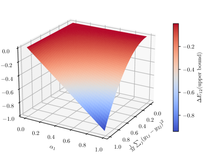
Figure 7: Upper bound for $\Delta E_{12}$ such that (20) is satisfied.

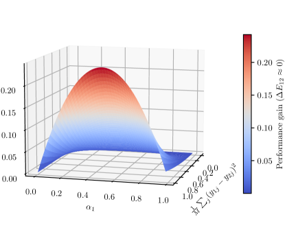
Figure 8: Estimated performance gain as a function of $\alpha_{1}$ and of the difference in output between the two NeRFs.

To validate our Mixture of Experts (MoE), we conducted a comparison with an ensemble of Neural Radiance Fields (NeRFs), where the output is determined by averaging the predictions of each NeRF model. Starting from a set of $M$ pre-trained models, an ensemble is built and is then fine-tuned. Averaging the outputs of NeRFs can notably enhance the quality of reconstruction. Let us assume we have two NeRFs, having as output respectively $\boldsymbol{y}_{1}$ and $\boldsymbol{y}_{2}$, while the ground truth is $\hat{\boldsymbol{y}}$. We can write an equality of their performance, in terms of mean-squared error:

$$E_{1} =\Delta E_{12}+E_{2}$$

$$\frac{1}{M}\sum_{j}(y_{1j}-\hat{y})^{2} =\Delta E_{12}+\frac{1}{M}\sum_{j}(y_{2j}-\hat{y})^{2}$$ (15)

where $\Delta E_{12}$ is the error gap between the two models and $M$ is the number of outputs on which the error is averaged. From (15) we can easily write

$$\frac{1}{M}\sum_{j}(y_{2j}^{2}-y_{1j}^{2})=\Delta E_{12}+\frac{2}{M}\sum_{j}\hat{y}(y_{2j}-y_{1j}).$$ (16)

Through ensembling, we desire the error $E_{\text{ens}}$ to be lower than either of the two other models. Without loss of generality, let us consider the case such that it is lower than the error of the first model:

$$E^{\text{ens}} <E_{1}$$

$$\frac{1}{M}\sum_{j}(\alpha_{1}y_{1j}+\alpha_{2}y_{2j}-\hat{y})^{2} <\frac{1}{M}\sum_{j}(y_{1j}-\hat{y})^{2}$$ (17)

where $\alpha_{1},\!\alpha_{2}$ are two weighting factors for the two NeRF’s outputs. If we expand (17) we obtain

$$\frac{1}{M}\sum_{j}(\alpha_{1}y_{1j}+ \alpha_{2}y_{2j})^{2}-y_{1j}^{2}<$$

$$\frac{2}{M}\sum_{j}\hat{y}\left[\alpha_{2}y_{2j}-(1-\alpha_{1})y_{1j}\right].$$ (18)

In order to plug (15) in (18), we need to impose $\alpha_{2}=1-\alpha_{1}$. Hence, we have

$$\frac{1}{M}\sum_{j} \left[\alpha_{1}y_{1j}+(1-\alpha_{1})y_{2j}\right]^{2}-y_{1j}^{2}<$$

$$(1-\alpha_{1})\left[\Delta E_{12}+\frac{1}{M}\sum_{j}(y_{2j}-\hat{y})^{2}\right].$$ (19)

By expanding and simplifying (19), we obtain

$$\frac{1}{M}\sum_{j}(\alpha_{1}^{2}-\alpha_{1})(y_{1j}-y_{2j})^{2}<(1-\alpha_{1})\Delta E_{12}.$$ (20)

Fig. 7 pictures the upper bound dictated by $\Delta E_{12}$ such that (20) is verified. Given that for (15) we never stated which of the two models has the lowest error, evidently if $\Delta E_{12}>0$, for $\alpha_{1}<1$ (20) is always verified. However, this is not anymore the case when $\Delta E_{12}<0$. In order to maximize the performance of the ensemble, we need to settle to the critical point of (20) (global maximum) with respect to $\alpha_{1}$, which is

$$\alpha_{1}=\frac{1-\Delta E_{12}}{2}.$$ (21)

If we assume $\Delta E_{12}$ being distributed as a random variable with zero means (this is a realistic assumption as we never stated which of the two models performs the best), evidently the best solution is for $\alpha_{1}=\frac{1}{2}$: Fig. 8 graphically evidences this.

8 Algorithm

We present an intuitive pseudo-algorithm outlining our Mixture of Experts framework. Our native implementation in PyTorch closely adheres to this algorithm.

Algorithm 1 Sparse MoE Trainining

1:$D$: dataset, $res$: resolution, $l$: number of pre-training iterations, $m$: number of training iterations, $M$: number of experts in the mixture, $k$: number of top points to select, $\lambda$: resolution-based aux-loss penalties, $W$: aux-loss weights

2:$experts\leftarrow$ create_experts($res$)

3:$experts\leftarrow$ pre_train($experts$, $l$)

4:$gate\leftarrow$ create_gate()

5:$moe\leftarrow$ build_moe($experts$, $gate$)

6:for $i\leftarrow 1$ to $m$ do

7:     $\mathbf{o}$, $\mathbf{d}$, $\mathbf{rgb}\leftarrow$ batch($D$)

8:     $\mathbf{x}\leftarrow$ sample_and_filter_points($\mathbf{o}$, $\mathbf{d}$)

9:     $G(\mathbf{x})\leftarrow$ $gate(\mathbf{x})$

10:     $topk\_idx$, $topk\_vals\leftarrow$ top-k($G(\mathbf{x}),k$)

11:     $\mathbf{\sigma_{s}}$, $\mathbf{c_{s}}$ $\leftarrow$ array()

12:     for $j\leftarrow 1$ to $M$ do

13:         $mask\leftarrow topk\_idx==j$

14:         $\mathbf{\sigma}$, $\mathbf{c}\leftarrow$ $experts[j](\mathbf{x}[mask],\mathbf{d})$

15:         $\mathbf{\sigma_{s}}[j]\leftarrow\sigma\cdot topk\_vals[mask]$

16:         ${\mathbf{c_{s}}[j]}\leftarrow\mathbf{c}\cdot topk\_vals[mask]$

17:     end for

18:     $\mathbf{\sigma_{f}}\leftarrow$ sum($\mathbf{\sigma}_{s}$)

19:     $\mathbf{c_{f}}\leftarrow$ sum($\mathbf{c_{s}}$)

20:     $\mathbf{colors}\leftarrow$ volume_rendering($\mathbf{\sigma_{f}}$, $\mathbf{c_{f}}$)

21:     $L_{\text{tot}}\leftarrow L_{\text{nerf}}(rgb,colors)+\lambda L_{\text{rw-aux}}(P(\mathbf{x}),W)$

22:     optimize($moe$)

23:end for

The initial phase involves independently training $M$ models at different resolutions for $m$ iterations. Given that we utilize Fast NeRFs, this phase tends to be rapid. Following this, we construct the Sparsely-Gated Mixture of Experts as outlined in lines 1-4 of the algorithm. The training of the MoE commences at line 4: Given a batch of rays, typically represented by a triplet (origin, direction, and ground truth color), points along the ray are sampled and appropriately filtered. Subsequently, for each point, a probability distribution is computed, indicating the confidence of the gate in assigning each point to each expert (line 8). Based on this probability, the points are delivered to the top-k experts, who calculate, for each point, the density and radiance, which are then multiplied by their corresponding probability value (lines 9-16). The density and radiance values are aggregated, yielding a single array of density and radiance (line 20). Finally, we proceed as usual by computing the pixel color using the volume rendering equation, calculating the loss, and optimizing both the gate and the experts. Our algorithm is tailored for a single GPU, but it can be readily extended to a multi-GPU environment, as the computation of the experts’ output can be parallelized.

9 Resolution Penalties

We experimented with different resolution-based penalties, namely: linear, geometric progression, and quadratic, defined as follows:

$$\text{linear}:w_{i+1}=w_{i}+k$$ (22)

$$\text{geom progr.}:w_{i}=\exp\left(\frac{\ln M}{M-1}\right)^{i}$$ (23)

$$\text{quadratic}:w_{i+1}=2*w_{i}$$ (24)

where $i\in[0,...,M-1]$ and $k=1$. Considering the results (Tab. 3), we opted for the geometric progression as it provides slightly better results. It’s worth noting how introducing such penalties further improves render quality compared to a standard auxiliary loss without resolution penalty (indicated as "none").

In Fig. 9, we provide a qualitative evaluation of experts’ specialization. With our strategy, we aim to utilize high-resolution models as sparingly as possible.

Table 3: Comparison among different penalty strategies

Strategy	Top-1		Top-2
	PSNR	$\|w\|_{0}$	PSNR	$\|w\|_{0}$
none	33.41	32	33.61	56
geom. progr.	33.43	26	33.74	39
quadratic	33.31	20	33.64	37
linear	33.41	32	33.63	36

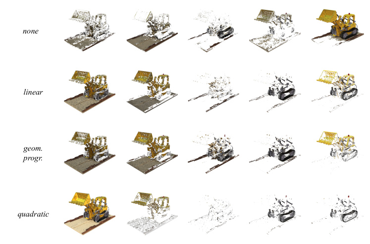
Figure 9: Per-experts outputs with a MoE of 5 NeRFs and top-2 with different resolution penalties. Experts’ output are ordered by increasing resolution.

10 Visualizing Experts Specialization

In Fig. 10 and 11 we show the output for each expert in the MoE with $M=5$, with respectively Top-$1$ and Top-$2$ function and resolution penalty.

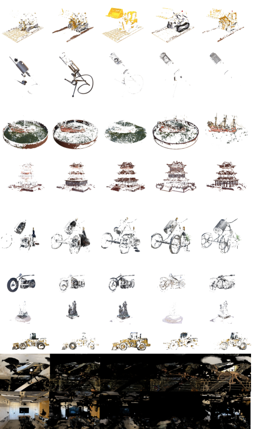
Figure 10: Per-expert output with Top-1 and 5 experts. Outputs are ordered from left to right by increasing experts’ resolution.

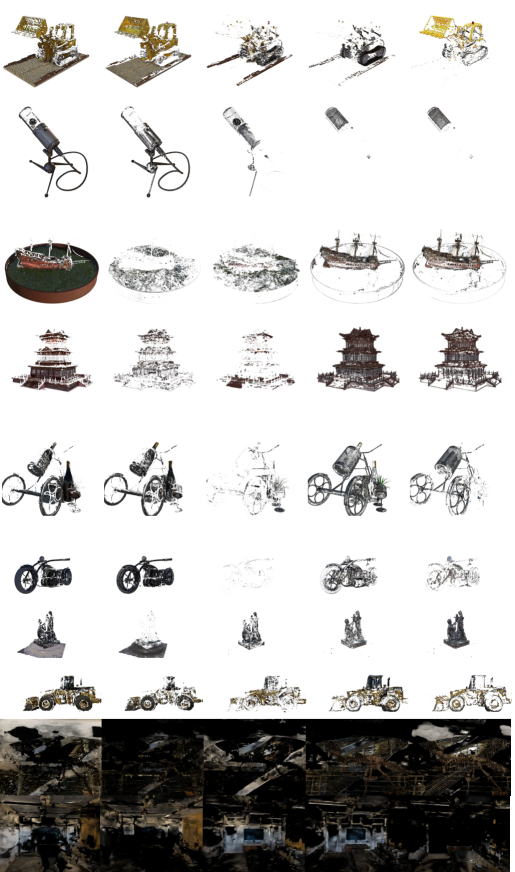
Figure 11: Per-expert output with Top-2 and 5 experts. Outputs are ordered from left to right by increasing experts’ resolution.

11 Comparison with SoTA Methods

Although our goal was to focus on fast models and improve reconstruction quality at a lower computational cost compared to their baseline counterparts, our method achieves comparable (and often superior) accuracy to explicit models. Table 4 presents a comparison with three state-of-the-art implicit models: Mip-NeRF [1], Mip-NeRF360 [2] and Zip-NeRF [3]. Training times refers to a single GPU configuration (NVIDIA A40). Mip-NeRF was trained for $1000000$ iterations; Mip-NeRF 360 and Zip-NeRF for $200000$ iterations.

Table 4: Comparison among boosted Fast-NeRF and implicit SoTA methods on Synthetic-NeRF dataset.

	PSNR	SSIM	Time
DVGO Top-1	33.43	0.964	21’
TensoRF Top-1	33.68	0.965	69’
iNGP Top-1	33.56	0.963	32’
DVGO Top-2	33.74	0.965	25’
TensoRF Top-2	34.09	0.968	76’
iNGP Top-2	33.83	0.965	34’
Mip-NeRF	33.09	0.961	16h
Mip-NeRF360	32.96	0.960	5h
Zip-NeRF	33.69	0.973	7h

12 Additional Results

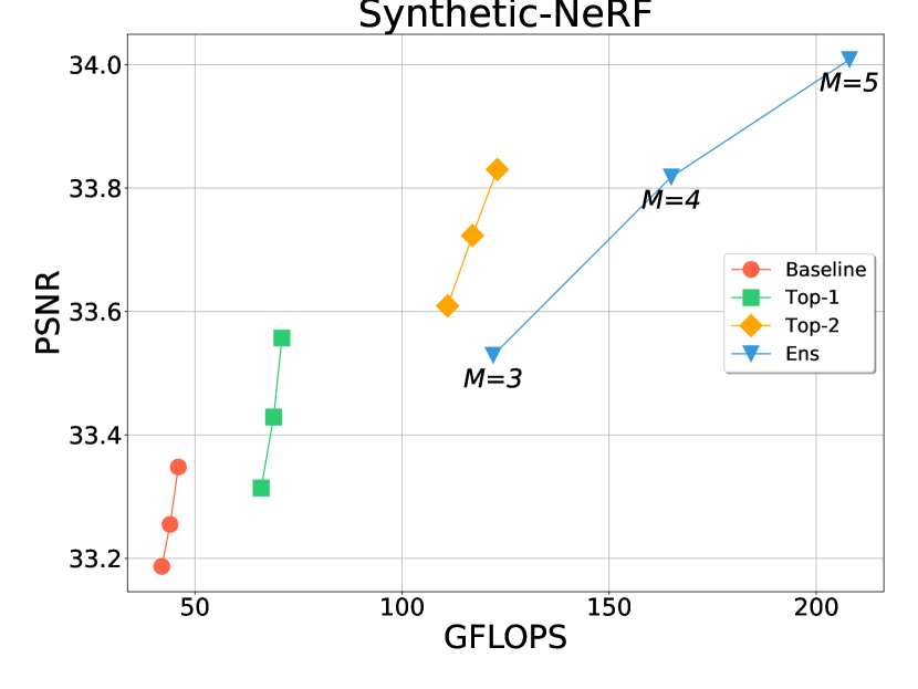
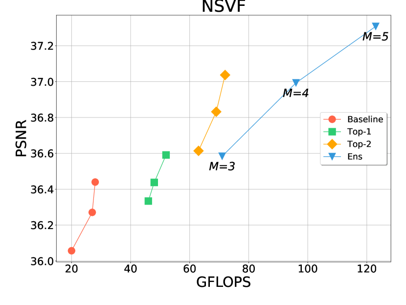
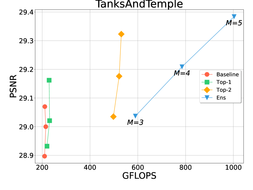
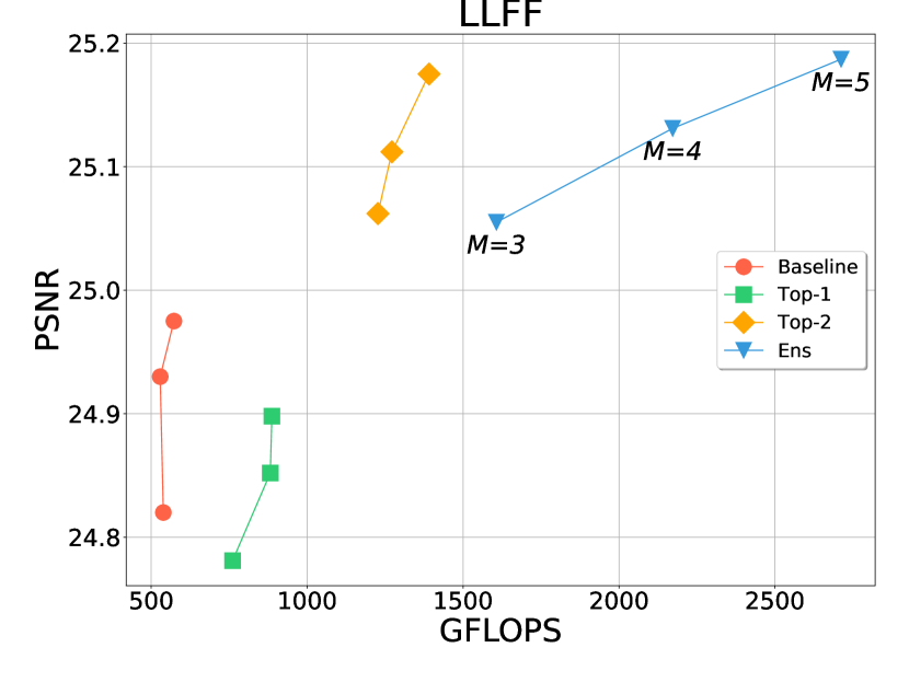
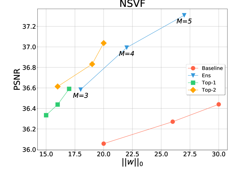
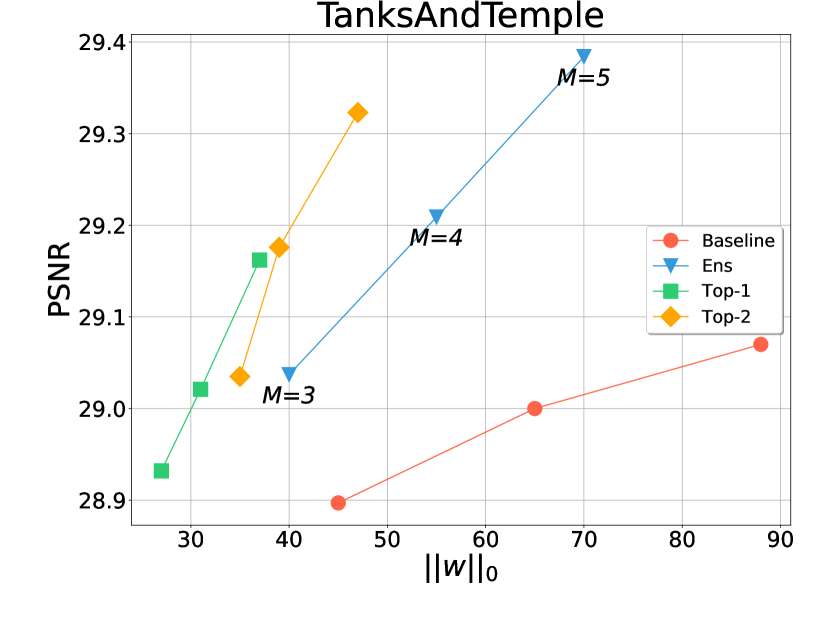
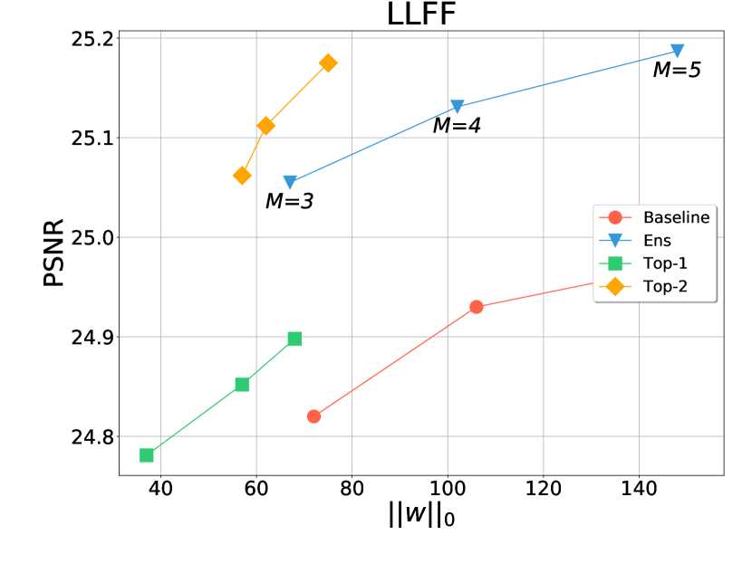
Figure 14: PSNR/GFLOPs and PSNR/$||w||_{0}$ plots for aggregated results with Instant-NGP.

In this section, we present additional results for DVGO, TensoRF, and Instant-NGP with varying values of $M={3,4,5}$. In Table 5 and Figure 12, we provide aggregated results for all the tested datasets on DVGO, including plots of PSNR/GLOPS and PSNR/$\|w\|_{0}$. Similarly, in Table 6 and Figure 13, we present the results for TensoRF. The results for Instant-NGP are shown in Table 7 and Figure 14.

Table 5: Aggregated results on DVGO

Dataset	Metrics	M=3				M=4				M=5
		baseline	Top-1	Top-2	Ens	baseline	Top-1	Top-2	Ens	baseline	Top-1	Top-2	Ens
Blender	PSNR$~{}\uparrow$	32.97	33.17	33.31	33.35	33.07	33.34	33.53	33.61	33.04	33.43	33.74	33.79
	SSIM $\uparrow$	0.962	0.962	0.964	0.964	0.963	0.963	0.965	0.965	0.963	0.964	0.965	0.966
	LPIPS $\downarrow$	0.026	0.026	0.025	0.025	0.025	0.025	0.024	0.023	0.026	0.024	0.022	0.022
	$\|w\|_{0}\downarrow$	29	17	25	32	57	20	33	59	99	26	39	97
	GFLOPs $\downarrow$	382	342	647	914	508	431	813	1529	635	499	940	2206
	time $\downarrow$	10’	12’	15’	15’	13’	16’	19’	23’	26’	20’	24’	32’
NSVF	PSNR$~{}\uparrow$	35.59	36.82	37.26	37.18	35.51	37.00	37.48	37.51	35.21	37.12	37.59	37.68
	SSIM $\uparrow$	0.979	0.982	0.984	0.984	0.979	0.983	0.985	0.985	0.977	0.984	0.986	0.986
	LPIPS $\downarrow$	0.014	0.010	0.009	0.009	0.014	0.010	0.008	0.008	0.015	0.009	0.008	0.007
	$\|w\|_{0}\downarrow$	29	18	23	32	60	23	32	60	95	27	43	100
	GFLOPs $\downarrow$	318	266	502	709	452	358	676	1271	564	430	811	1903
	time $\downarrow$	7’	13’	16’	16’	22’	17’	21’	25’	12’	21’	25’	35’
TaT	PSNR$~{}\uparrow$	28.59	28.93	29.10	29.11	28.71	29.05	29.21	29.27	28.93	29.14	29.27	29.37
	SSIM $\uparrow$	0.919	0.921	0.925	0.926	0.921	0.923	0.927	0.930	0.927	0.925	0.929	0.932
	LPIPS $\downarrow$	0.131	0.115	0.113	0.113	0.121	0.110	0.108	0.107	0.107	0.108	0.105	0.103
	$\|w\|_{0}\downarrow$	17	11	18	25	30	15	22	43	74	16	26	65
	GFLOPs $\downarrow$	1299	1223	2310	3263	1547	1463	2761	5193	2666	1626	3066	7198
	time $\downarrow$	10’	15’	18’	18’	18’	19’	23’	27’	22’	25’	28’	38’
LLFF	PSNR$~{}\uparrow$	26.20	26.05	26.33	26.31	26.29	26.30	26.51	26.53	26.24	26.43	26.62	26.65
	SSIM $\uparrow$	0.832	0.823	0.831	0.834	0.832	0.830	0.837	0.841	0.831	0.832	0.839	0.843
	LPIPS $\downarrow$	0.141	0.130	0.120	0.123	0.137	0.117	0.116	0.112	0.136	0.115	0.111	0.107
	$\|w\|_{0}\downarrow$	19	12	23	28	33	19	29	59	62	26	40	113
	GFLOPs $\downarrow$	976	844	1408	1693	1250	1162	1931	3079	1678	1514	2508	4972
	time $\downarrow$	12’	14’	16’	13’	16’	20’	23’	23’	24’	28’	32’	36’

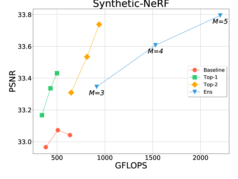
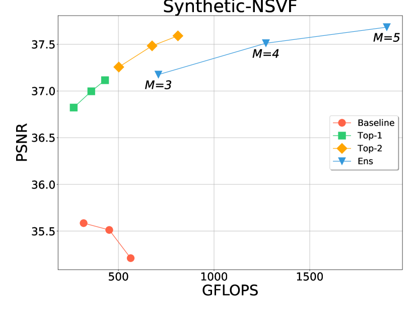
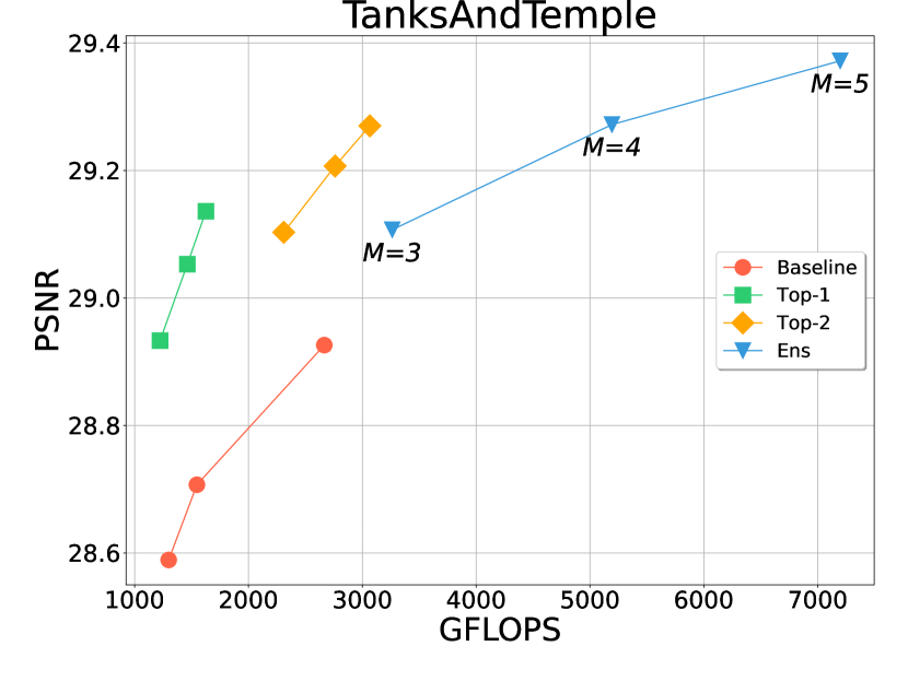
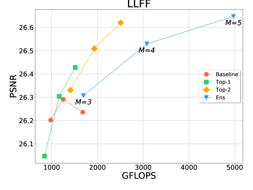
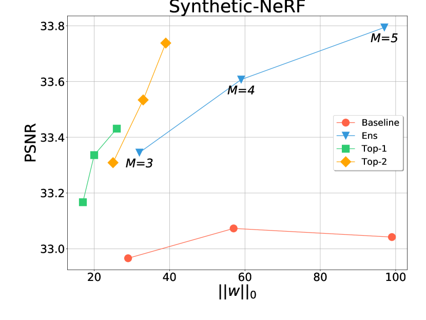
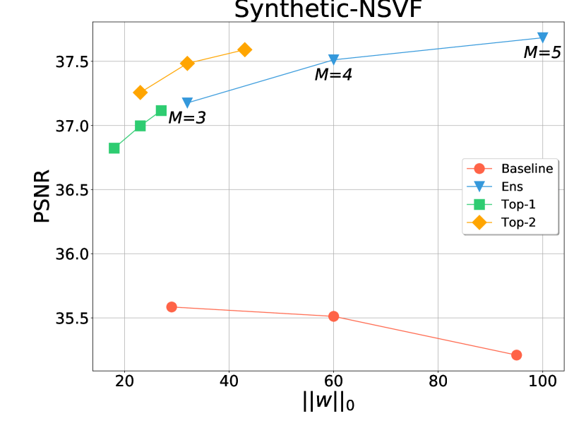
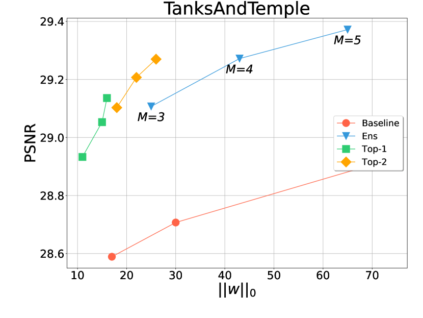
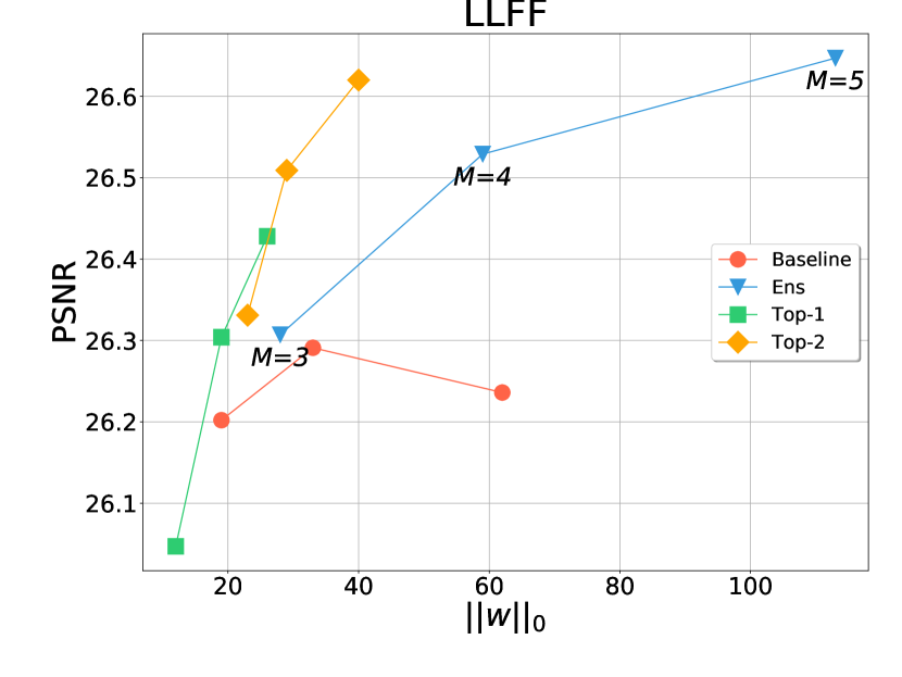
Figure 12: PSNR/GFLOPs and PSNR/$||w||_{0}$ plots for DVGO aggregated results.

Table 6: Aggregated results on TensoRF

Dataset	Metrics	M=3				M=4				M=5
		baseline	Top-1	Top-2	Ens	baseline	Top-1	Top-2	Ens	baseline	Top-1	Top-2	Ens
Blender	PSNR$~{}\uparrow$	33.30	33.45	33.83	33.66	33.19	33.58	33.99	33.83	32.98	33.68	34.09	34.00
	SSIM $\uparrow$	0.962	0.965	0.967	0.966	0.962	0.966	0.968	0.967	0.958	0.965	0.968	0.968
	LPIPS $\downarrow$	0.027	0.025	0.024	0.024	0.027	0.024	0.022	0.023	0.029	0.024	0.021	0.022
	$\|w\|_{0}\downarrow$	15	11	15	18	26	16	23	31	40	24	33	49
	GFLOPs $\downarrow$	600	520	958	1327	753	641	1179	1770	886	732	1344	2214
	time $\downarrow$	29’	40’	44’	40’	36’	55’	61’	53’	44’	69’	76’	70’
NSVF	PSNR$~{}\uparrow$	36.91	36.98	37.58	37.54	36.95	37.18	37.81	37.85	36.70	37.40	37.98	38.08
	SSIM $\uparrow$	0.982	0.983	0.985	0.985	0.981	0.983	0.986	0.986	0.981	0.984	0.986	0.987
	LPIPS $\downarrow$	0.011	0.010	0.009	0.009	0.012	0.010	0.008	0.008	0.013	0.009	0.008	0.008
	$\|w\|_{0}\downarrow$	17	10	15	20	28	19	26	35	42	28	38	54
	GFLOPs $\downarrow$	477	414	761	1055	591	504	924	1408	706	575	1053	1763
	time $\downarrow$	29’	45’	44’	40’	36’	58’	60’	56’	46’	75’	75’	75’
TaT	PSNR$~{}\uparrow$	28.65	28.79	29.00	28.95	28.55	28.77	29.05	29.04	28.44	28.78	29.14	29.11
	SSIM $\uparrow$	0.906	0.922	0.924	0.925	0.906	0.924	0.927	0.927	0.905	0.924	0.929	0.928
	LPIPS $\downarrow$	0.136	0.112	0.111	0.113	0.130	0.106	0.104	0.113	0.123	0.106	0.099	0.109
	$\|w\|_{0}\downarrow$	3	5	8	11	5	7	11	49	7	9	15	80
	GFLOPs $\downarrow$	2379	2151	3959	5481	2915	2475	4549	7311	3567	2791	5126	9146
	time $\downarrow$	40’	41’	43’	44’	54’	53’	59’	72’	72’	70’	78’	101’
LLFF	PSNR$~{}\uparrow$	26.60	26.58	26.86	26.80	26.72	26.73	26.98	27.00	26.71	26.73	27.09	27.10
	SSIM $\uparrow$	0.834	0.835	0.841	0.840	0.836	0.839	0.843	0.843	0.835	0.836	0.862	0.864
	LPIPS $\downarrow$	0.127	0.117	0.110	0.116	0.118	0.112	0.105	0.107	0.114	0.111	0.101	0.101
	$\|w\|_{0}\downarrow$	9	5	6	8	13	6	10	14	19	11	16	23
	GFLOPs $\downarrow$	3111	2016	3707	5100	3779	2576	4731	8660	4542	3226	5921	13522
	time $\downarrow$	36’	27’	31’	31’	49’	37’	43’	49’	58’	49’	57’	68’

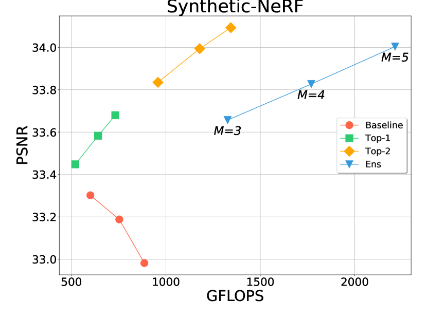
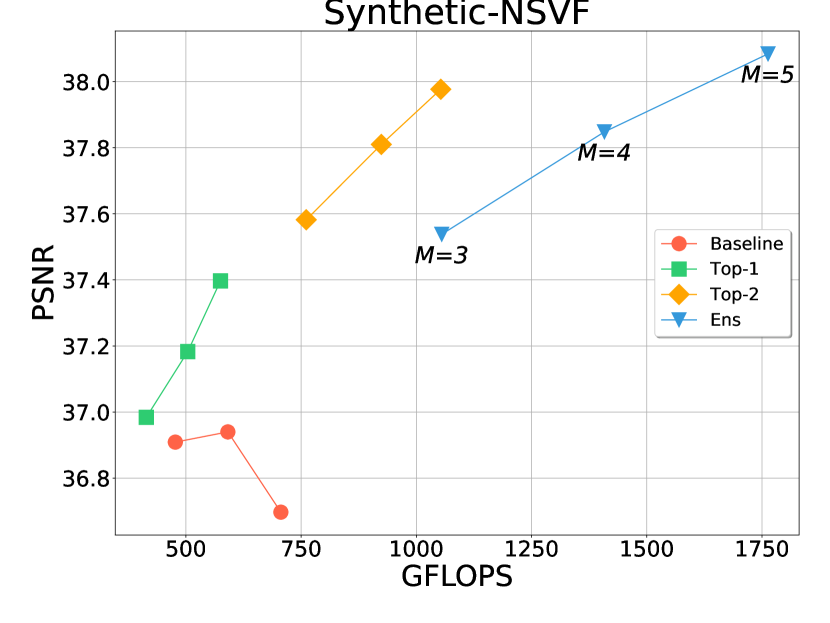
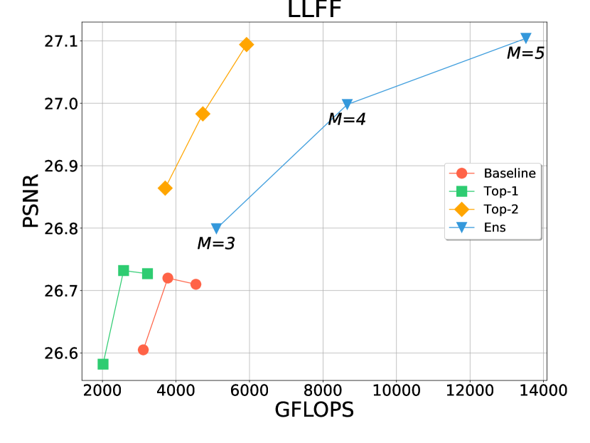
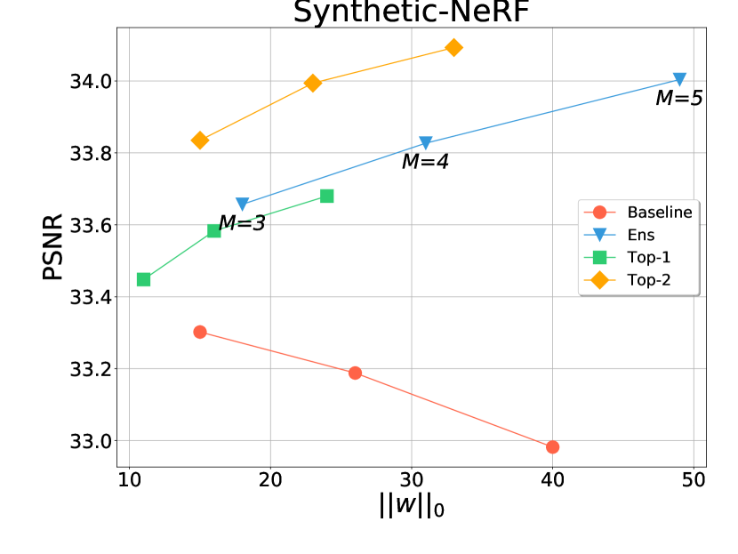
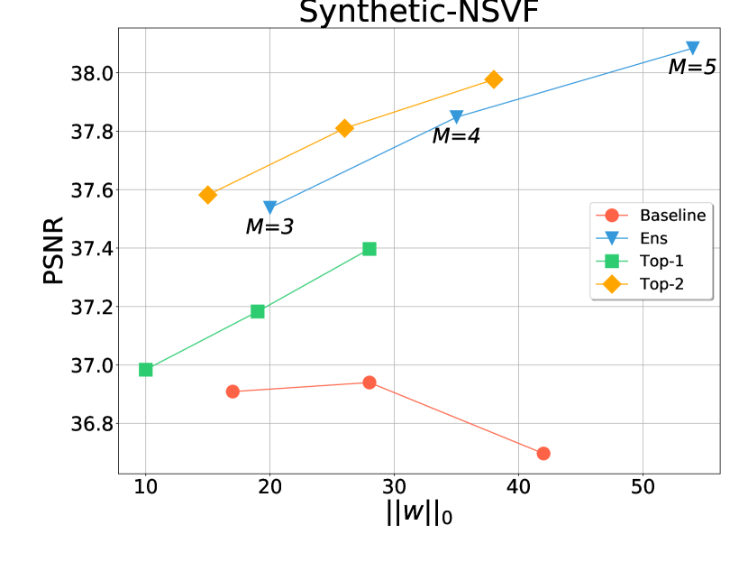
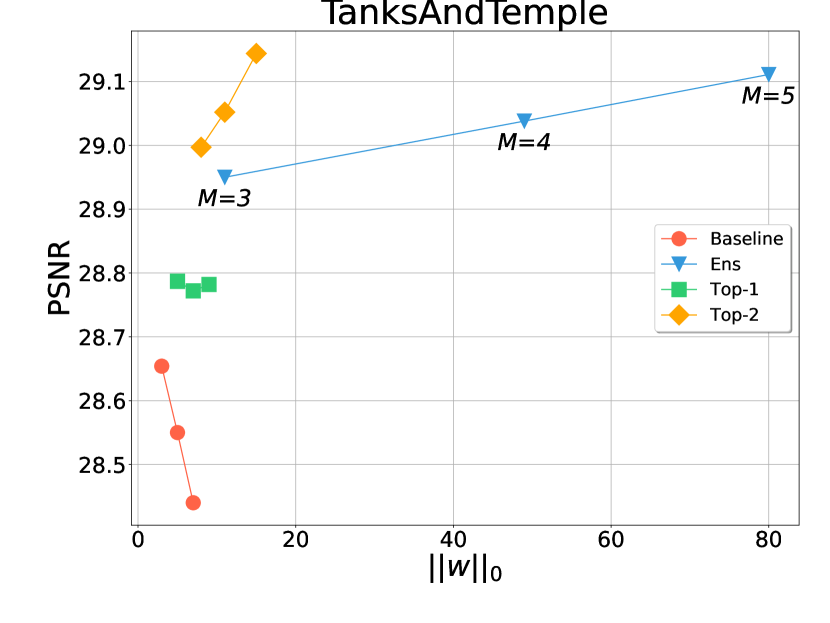
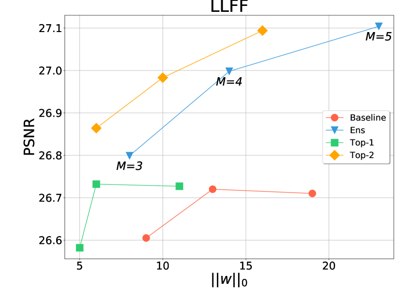
Figure 13: PSNR/GFLOPs and PSNR/$||w||_{0}$ plots for aggregated results with TensoRF.

Table 7: Aggregated results on Instant-NGP

Dataset	Metrics	M=3				M=4				M=5
		baseline	Top-1	Top-2	Ens	baseline	Top-1	Top-2	Ens	baseline	Top-1	Top-2	Ens
Blender	PSNR$~{}\uparrow$	33.19	33.31	33.61	33.53	33.25	33.43	33.72	33.82	33.35	33.56	33.83	34.01
	SSIM $\uparrow$	0.961	0.962	0.962	0.963	0.962	0.963	0.964	0.964	0.963	0.963	0.965	0.966
	LPIPS $\downarrow$	0.027	0.049	0.047	0.047	0.026	0.046	0.045	0.044	0.025	0.045	0.043	0.042
	$\|w\|_{0}\downarrow$	20	13	15	18	26	14	19	22	31	17	21	26
	GFLOPs $\downarrow$	42	66	111	122	44	69	117	165	46	71	123	208
	time $\downarrow$	7’	23’	26’	27’	9’	27’	30’	30’	11’	32’	34’	37’
NSVF	PSNR$~{}\uparrow$	36.06	36.33	36.61	36.58	36.27	36.44	36.83	36.99	36.44	36.59	37.04	37.31
	SSIM $\uparrow$	0.981	0.981	0.982	0.982	0.982	0.983	0.983	0.984	0.983	0.983	0.984	0.985
	LPIPS $\downarrow$	0.012	0.024	0.024	0.023	0.011	0.023	0.023	0.022	0.010	0.023	0.022	0.020
	$\|w\|_{0}\downarrow$	20	15	16	18	26	16	19	22	30	17	20	27
	GFLOPs $\downarrow$	20	46	63	71	27	48	69	96	28	52	72	123
	time $\downarrow$	7’	24’	25’	27’	8’	28’	29’	32’	10’	31’	33’	34’
TaT	PSNR$~{}\uparrow$	28.90	28.93	29.04	29.04	29.00	29.02	29.18	29.21	29.07	29.16	29.32	29.38
	SSIM $\uparrow$	0.919	0.920	0.918	0.922	0.922	0.924	0.928	0.929	0.924	0.927	0.929	0.930
	LPIPS $\downarrow$	0.107	0.131	0.130	0.129	0.105	0.127	0.125	0.124	0.101	0.125	0.124	0.121
	$\|w\|_{0}\downarrow$	45	27	35	40	65	31	39	55	88	37	47	70
	GFLOPs $\downarrow$	210	220	498	590	215	231	522	785	211	229	531	1003
	time $\downarrow$	9’	30’	30’	32’	11’	33’	34’	34’	14’	37’	39’	45’
LLFF	PSNR$~{}\uparrow$	24.82	24.78	25.06	25.06	24.93	24.85	25.11	25.13	24.97	24.90	25.17	25.19
	SSIM $\uparrow$	0.764	0.762	0.772	0.772	0.763	0.765	0.777	0.776	0.764	0.763	0.777	0.778
	LPIPS $\downarrow$	0.134	0.244	0.241	0.240	0.130	0.243	0.238	0.237	0.128	0.239	0.237	0.234
	$\|w\|_{0}\downarrow$	72	37	57	67	106	57	62	102	152	68	75	148
	GFLOPs $\downarrow$	539	761	1227	1607	529	882	1272	2172	573	887	1391	2712
	time $\downarrow$	14’	20’	22’	22’	18’	28’	30’	29’	24’	25’	46’	42’

Table 8: DVGO results on Synthetic-NeRF

Method	Scene	M=3					M=4					M=5
		PSNR	SSIM	LPIPS	$\|w\||_{0}\$	GFLOPs	PSNR	SSIM	LPIPS	$\|w\||_{0}\$	GFLOPs	PSNR	SSIM	LPIPS	$\|w\||_{0}\$	GFLOPs
Baseline	Lego	35.99	0.981	0.009	9	224	35.85	0.980	0.009	13	324	35.52	0.978	0.010	26	929
	Mic	35.47	0.990	0.006	7	85	36.24	0.991	0.005	9	127	36.68	0.992	0.005	18	845
	Chair	35.70	0.985	0.009	9	96	35.95	0.986	0.009	12	175	36.01	0.986	0.009	23	703
	Hotdog	37.09	0.982	0.013	11	436	36.89	0.981	0.014	15	588	36.67	0.981	0.015	30	820
	Ficus	33.90	0.983	0.012	8	121	33.80	0.982	0.013	12	145	33.86	0.982	0.014	22	773
	Drums	25.81	0.935	0.051	8	258	25.97	0.937	0.049	11	320	25.94	0.936	0.049	20	1048
	Materials	29.50	0.948	0.025	12	731	29.33	0.945	0.029	17	975	29.07	0.940	0.035	32	806
	Ship	30.27	0.895	0.083	13	1107	30.56	0.898	0.074	18	1412	30.59	0.896	0.069	35	790
	avg	32.97	0.962	0.026	10	382	33.07	0.963	0.025	13	508	33.04	0.961	0.026	26	839
Top-1	Lego	36.40	0.982	0.008	13	200	36.45	0.982	0.008	15	252	36.52	0.983	0.008	20	311
	Mic	35.34	0.990	0.006	4	74	36.08	0.991	0.005	5	96	36.47	0.992	0.004	6	119
	Chair	35.81	0.984	0.009	6	81	36.01	0.985	0.008	6	108	36.06	0.985	0.008	9	151
	Hotdog	37.35	0.982	0.013	18	382	37.39	0.982	0.013	23	491	37.35	0.982	0.013	28	574
	Ficus	34.37	0.983	0.012	13	115	34.47	0.984	0.012	15	136	34.45	0.984	0.012	20	147
	Drums	25.80	0.932	0.054	10	251	25.91	0.934	0.051	11	291	26.00	0.935	0.049	16	327
	Materials	29.95	0.952	0.025	39	643	29.91	0.952	0.025	49	824	29.72	0.950	0.026	59	963
	Ship	30.32	0.892	0.082	29	994	30.53	0.895	0.076	40	1247	30.75	0.897	0.071	47	1395
	avg	33.17	0.962	0.026	17	342	33.34	0.963	0.025	20	431	33.41	0.964	0.024	26	499
Top-2	Lego	36.59	0.983	0.008	20	378	36.80	0.983	0.008	26	476	36.89	0.983	0.007	31	587
	Mic	35.49	0.990	0.005	6	140	36.43	0.992	0.004	9	181	36.98	0.993	0.004	8	225
	Chair	36.16	0.986	0.008	8	153	36.41	0.987	0.007	11	204	36.54	0.987	0.007	12	285
	Hotdog	37.50	0.983	0.013	27	721	37.68	0.984	0.011	38	926	37.78	0.984	0.011	48	1083
	Ficus	34.20	0.983	0.012	22	217	34.28	0.983	0.011	21	256	34.45	0.984	0.011	26	277
	Drums	25.98	0.936	0.050	15	475	26.05	0.937	0.048	22	548	26.21	0.938	0.046	21	616
	Materials	29.98	0.953	0.023	53	1214	29.95	0.953	0.023	74	1555	29.99	0.954	0.022	87	1815
	Ship	30.57	0.897	0.084	47	1878	30.78	0.900	0.076	60	2354	31.07	0.901	0.071	80	2631
	avg	33.31	0.964	0.025	25	647	33.53	0.965	0.024	33	813	33.74	0.965	0.022	39	940
Ens	Lego	36.54	0.983	0.008	27	534	36.75	0.983	0.007	47	895	36.82	0.984	0.007	76	1377
	Mic	35.45	0.990	0.006	7	198	36.22	0.992	0.005	13	340	36.77	0.992	0.004	21	529
	Chair	36.24	0.986	0.008	13	215	36.53	0.987	0.008	23	384	36.67	0.988	0.007	36	670
	Hotdog	37.72	0.984	0.011	39	1019	37.79	0.985	0.011	75	1742	37.85	0.985	0.011	127	2542
	Ficus	34.14	0.983	0.010	24	306	34.42	0.984	0.010	42	482	34.61	0.985	0.009	64	651
	Drums	26.09	0.936	0.050	20	671	26.21	0.937	0.048	35	1031	26.39	0.940	0.045	56	1445
	Materials	30.05	0.954	0.021	71	1715	30.11	0.955	0.019	136	2925	30.19	0.956	0.019	227	4262
	Ship	30.53	0.897	0.081	53	2653	30.82	0.900	0.075	102	4428	31.06	0.903	0.070	169	6176
	avg	33.35	0.964	0.025	32	914	33.61	0.965	0.023	59	1529	33.79	0.966	0.022	97	2206

Table 9: Per-scene results on NSVF with DVGO

Method	Scene	M=3					M=4					M=5
		PSNR	SSIM	LPIPS	$\|w\||_{0}\$	GFLOPs	PSNR	SSIM	LPIPS	$\|w\||_{0}\$	GFLOPs	PSNR	SSIM	LPIPS	$\|w\||_{0}\$	GFLOPs
Baseline	Bike	38.13	0.991	0.004	16	269	37.70	0.990	0.004	32	369	37.25	0.989	0.005	48	448
	Lifestyle	34.27	0.969	0.021	20	369	34.34	0.969	0.021	42	505	34.24	0.968	0.022	65	619
	Palace	36.59	0.974	0.015	21	189	37.01	0.976	0.013	43	264	36.90	0.975	0.012	66	319
	Robot	37.24	0.993	0.004	31	385	37.07	0.992	0.004	64	585	36.56	0.991	0.004	100	730
	Spaceship	36.53	0.983	0.016	58	399	35.63	0.979	0.022	113	536	34.78	0.974	0.028	179	662
	Streamtrain	36.17	0.985	0.011	37	263	35.53	0.982	0.013	79	369	34.87	0.978	0.017	132	473
	Toad	34.67	0.977	0.018	20	182	35.28	0.980	0.014	40	252	35.42	0.981	0.013	61	314
	Wineholder	31.08	0.959	0.025	30	487	31.54	0.963	0.022	64	731	31.67	0.963	0.022	106	945
	avg	35.59	0.979	0.014	29	318	35.51	0.979	0.014	60	452	35.21	0.977	0.015	95	564
Top-1	Bike	39.68	0.993	0.003	13	160	39.60	0.993	0.003	16	213	39.55	0.993	0.003	22	255
	Lifestyle	35.25	0.971	0.018	15	307	35.27	0.972	0.016	21	416	35.37	0.973	0.015	25	467
	Palace	37.53	0.977	0.010	21	426	37.97	0.980	0.010	26	549	38.24	0.981	0.008	28	681
	Robot	38.79	0.995	0.003	13	158	39.07	0.995	0.002	16	205	39.11	0.995	0.002	23	245
	Spaceship	38.43	0.988	0.009	20	238	38.43	0.988	0.010	24	296	38.17	0.987	0.011	33	356
	Streamtrain	37.39	0.990	0.007	36	337	37.35	0.990	0.007	50	449	37.27	0.990	0.007	53	533
	Toad	35.32	0.979	0.015	11	257	35.88	0.982	0.012	16	434	36.58	0.984	0.010	19	539
	Wineholder	32.18	0.965	0.019	11	241	32.41	0.967	0.018	13	303	32.67	0.969	0.016	18	364
	avg	36.82	0.982	0.010	18	266	37.00	0.983	0.010	23	358	37.12	0.984	0.009	27	430
Top-2	Bike	40.09	0.994	0.002	18	303	40.08	0.994	0.002	25	403	40.01	0.994	0.002	30	481
	Lifestyle	35.51	0.974	0.015	17	580	35.65	0.975	0.015	26	785	35.67	0.975	0.014	33	881
	Palace	37.94	0.980	0.011	30	806	38.50	0.982	0.009	45	1036	38.80	0.983	0.008	53	1283
	Robot	39.29	0.995	0.002	19	300	39.43	0.995	0.002	26	387	39.46	0.995	0.002	35	462
	Spaceship	38.98	0.989	0.007	31	449	39.00	0.990	0.007	35	560	39.03	0.990	0.007	48	671
	Streamtrain	37.62	0.991	0.007	40	638	37.57	0.991	0.007	66	848	37.54	0.991	0.007	95	1005
	Toad	36.19	0.982	0.012	12	486	36.80	0.985	0.010	17	819	37.16	0.985	0.009	25	1016
	Wineholder	32.43	0.967	0.018	16	456	32.83	0.970	0.015	18	572	33.06	0.971	0.014	27	686
	avg	37.26	0.984	0.009	23	502	37.48	0.985	0.008	32	676	37.59	0.986	0.008	43	811
Ens	Bike	39.84	0.993	0.002	24	428	40.00	0.994	0.002	44	758	39.95	0.994	0.002	70	1130
	Lifestyle	35.50	0.974	0.015	23	819	35.67	0.976	0.013	43	1477	35.75	0.976	0.012	68	2069
	Palace	37.98	0.980	0.010	38	1138	38.66	0.983	0.008	69	1948	39.03	0.984	0.007	115	3012
	Robot	39.08	0.995	0.002	24	423	39.33	0.995	0.002	45	727	39.43	0.995	0.002	74	1084
	Spaceship	39.03	0.990	0.007	44	635	39.15	0.990	0.007	81	1052	39.22	0.990	0.007	137	1576
	Streamtrain	37.49	0.991	0.007	60	901	37.52	0.991	0.007	115	1595	37.50	0.990	0.007	192	2359
	Toad	36.28	0.983	0.011	24	686	37.05	0.986	0.009	50	1540	37.53	0.987	0.008	86	2385
	Wineholder	32.22	0.967	0.018	19	644	32.70	0.970	0.016	35	1075	33.06	0.972	0.014	56	1610
	avg	37.18	0.984	0.009	32	709	37.51	0.985	0.008	60	1271	37.68	0.986	0.007	100	1903

Table 10: Per-scene results on TanksAndTemple with DVGO

Method	Scene	M=3					M=4					M=5
		PSNR	SSIM	LPIPS	$\|w\||_{0}\$	GFLOPs	PSNR	SSIM	LPIPS	$\|w\||_{0}\$	GFLOPs	PSNR	SSIM	LPIPS	$\|w\||_{0}\$	GFLOPs
Baseline	Ignatius	28.39	0.95	0.076	20	1588	28.55	0.951	0.07	35	1755	27.86	0.873	0.207	84	3490
	Caterpillar	26.06	0.911	0.137	9	1298	26.08	0.912	0.129	31	1012	27.68	0.924	0.102	59	1592
	Family	33.76	0.964	0.057	23	1293	33.75	0.964	0.053	20	1647	26.13	0.914	0.119	51	2561
	Barn	27.28	0.853	0.258	16	822	27.61	0.860	0.236	20	1588	28.52	0.951	0.068	89	3088
	Truck	27.45	0.915	0.126	18	1493	27.55	0.920	0.115	47	1735	34.43	0.97	0.039	86	2599
	avg	28.59	0.919	0.131	17	1299	28.71	0.921	0.121	31	1547	28.92	0.926	0.107	74	2666
Top-1	Ignatius	28.18	0.947	0.073	11	796	28.28	0.948	0.071	12	926	28.36	0.949	0.070	14	1044
	Caterpillar	26.45	0.914	0.121	11	1265	26.55	0.914	0.119	14	1462	26.59	0.916	0.117	14	1716
	Family	34.5	0.968	0.049	11	1140	34.67	0.969	0.046	15	1457	34.75	0.97	0.044	18	1714
	Barn	27.85	0.859	0.223	12	1384	27.98	0.865	0.21	16	1681	28.18	0.868	0.204	18	1656
	Truck	27.69	0.918	0.11	12	1527	27.78	0.921	0.105	15	1789	27.8	0.921	0.104	18	2002
	avg	28.93	0.921	0.115	11	1223	29.05	0.923	0.110	15	1463	29.14	0.925	0.108	16	1626
Top-2	Ignatius	28.21	0.949	0.074	17	1505	28.27	0.950	0.071	21	1747	28.27	0.951	0.069	28	1969
	Caterpillar	26.66	0.918	0.12	16	2390	26.72	0.920	0.117	19	2759	26.78	0.921	0.114	24	3235
	Family	34.75	0.97	0.048	17	2155	34.92	0.972	0.045	20	2750	35	0.972	0.043	24	3232
	Barn	28.14	0.866	0.212	19	2616	28.27	0.871	0.202	26	3173	28.42	0.874	0.195	27	3122
	Truck	27.75	0.921	0.11	19	2885	27.84	0.924	0.105	23	3377	27.88	0.925	0.101	26	3773
	avg	29.10	0.925	0.113	18	2310	29.21	0.927	0.108	22	2761	29.27	0.929	0.105	26	3066
Ens	Ignatius	28.26	0.95	0.076	21	2126	28.36	0.953	0.072	37	3286	28.4	0.954	0.07	57	4622
	Caterpillar	26.66	0.919	0.122	20	3377	26.85	0.923	0.118	30	5189	26.94	0.925	0.113	46	7593
	Family	34.72	0.971	0.047	28	3045	34.93	0.973	0.044	50	5173	35.06	0.974	0.042	82	7588
	Barn	28.13	0.868	0.209	27	3695	28.32	0.874	0.197	48	5968	28.51	0.879	0.19	68	7328
	Truck	27.76	0.923	0.111	27	4075	27.89	0.927	0.104	46	6350	27.95	0.93	0.101	71	8857
	avg	29.11	0.926	0.113	25	3263	29.27	0.930	0.107	43	5193	29.37	0.932	0.103	65	7198

Table 11: Per-scene results on LLFF with DVGO

Method	Scene	M=3					M=4					M=5
		PSNR	SSIM	LPIPS	$\|w\||_{0}\$	GFLOPs	PSNR	SSIM	LPIPS	$\|w\||_{0}\$	GFLOPs	PSNR	SSIM	LPIPS	$\|w\||_{0}\$	GFLOPs
Baseline	Fern	24.89	0.816	0.166	28	1062	24.76	0.816	0.161	49	1382	24.58	0.810	0.160	95	1859
	Flower	27.51	0.850	0.132	16	1018	27.65	0.854	0.127	28	1295	27.67	0.856	0.122	53	1690
	Fortress	29.91	0.859	0.121	8	640	29.42	0.831	0.143	16	907	29.38	0.821	0.149	36	1407
	Horns	27.55	0.863	0.142	19	1017	27.83	0.874	0.129	32	1258	27.86	0.878	0.120	60	1641
	Leaves	20.96	0.737	0.181	21	915	21.06	0.744	0.167	36	1187	21.08	0.748	0.156	67	1547
	Orchids	20.40	0.683	0.186	29	1354	20.51	0.683	0.181	49	1684	20.42	0.680	0.179	86	2096
	Room	31.36	0.944	0.107	13	922	31.75	0.947	0.101	22	1154	31.65	0.937	0.114	43	1613
	Trex	27.04	0.904	0.094	16	877	27.34	0.910	0.089	29	1136	27.24	0.913	0.085	57	1579
	avg	26.20	0.832	0.141	19	976	26.29	0.832	0.137	33	1251	26.24	0.831	0.136	62	1679
Top-1	Fern	24.31	0.798	0.162	16	932	24.45	0.804	0.149	27	1299	24.48	0.806	0.150	39	1518
	Flower	27.44	0.846	0.115	12	872	27.53	0.851	0.107	19	1175	27.72	0.858	0.099	26	1518
	Fortress	29.71	0.836	0.131	7	618	29.96	0.847	0.113	10	812	29.93	0.845	0.116	16	1531
	Horns	27.68	0.861	0.129	12	957	28.08	0.877	0.107	18	1277	28.29	0.883	0.101	24	1460
	Leaves	20.76	0.735	0.152	14	814	20.91	0.745	0.139	22	1109	20.95	0.747	0.131	31	1615
	Orchids	19.68	0.658	0.165	17	986	19.71	0.659	0.159	29	1423	19.73	0.655	0.158	37	1660
	Room	31.64	0.943	0.098	9	840	32.08	0.947	0.092	13	1193	32.40	0.947	0.093	17	1522
	Trex	27.17	0.903	0.085	10	734	27.71	0.914	0.073	15	1006	27.92	0.918	0.067	21	1291
	avg	26.05	0.823	0.130	12	844	26.30	0.830	0.117	19	1162	26.43	0.832	0.115	26	1514
Top-2	Fern	24.34	0.801	0.156	30	1555	24.57	0.811	0.148	43	2159	24.36	0.808	0.144	62	2815
	Flower	27.83	0.858	0.108	21	1454	27.86	0.861	0.105	27	1953	27.97	0.864	0.100	37	2467
	Fortress	30.34	0.867	0.098	14	1030	30.18	0.859	0.105	16	1349	30.18	0.860	0.105	28	2123
	Horns	28.05	0.874	0.118	24	1596	28.42	0.883	0.108	27	2123	28.69	0.890	0.100	30	2609
	Leaves	20.74	0.737	0.151	27	1358	20.97	0.750	0.141	38	1844	20.99	0.752	0.133	51	2351
	Orchids	19.64	0.654	0.166	31	1644	19.66	0.656	0.159	35	2366	19.70	0.658	0.156	55	3017
	Room	32.25	0.950	0.087	17	1401	32.51	0.952	0.087	22	1983	32.96	0.955	0.081	29	2506
	Trex	27.45	0.910	0.079	18	1224	27.90	0.919	0.072	22	1671	28.07	0.923	0.068	32	2174
	avg	26.33	0.831	0.120	23	1408	26.51	0.837	0.116	29	1931	26.62	0.839	0.111	40	2508
Ens	Fern	24.55	0.806	0.155	38	1870	24.69	0.811	0.144	83	3444	24.72	0.813	0.143	162	5582
	Flower	27.70	0.858	0.113	26	1748	27.85	0.863	0.107	53	3115	27.95	0.864	0.102	97	4892
	Fortress	30.22	0.869	0.094	16	1239	30.43	0.874	0.081	32	2151	30.24	0.874	0.096	72	4208
	Horns	27.94	0.876	0.117	31	1919	28.29	0.890	0.099	64	3385	28.56	0.891	0.087	115	5174
	Leaves	20.81	0.739	0.160	31	1633	20.95	0.749	0.146	65	2940	21.01	0.750	0.137	123	4661
	Orchids	19.86	0.666	0.173	39	1977	19.90	0.667	0.167	84	3774	19.95	0.667	0.163	154	5983
	Room	32.15	0.951	0.087	21	1685	32.57	0.955	0.080	45	3162	33.03	0.965	0.075	83	4969
	Trex	27.20	0.908	0.082	23	1471	27.56	0.917	0.074	49	2664	27.72	0.917	0.070	94	4310
	avg	26.31	0.834	0.123	28	1693	26.53	0.841	0.112	59	3079	26.65	0.843	0.109	113	4972

Table 12: Per-scene results on Synthetic-NeRF with TensorF

Method	Scene	M=3					M=4					M=5
		PSNR	SSIM	LPIPS	$\|w\||_{0}$	GFLOPs	PSNR	SSIM	LPIPS	$\|w\||_{0}$	GFLOPs	PSNR	SSIM	LPIPS	$\|w\||_{0}$	GFLOPs
Baseline	Lego	36.85	0.986	0.006	15	376	36.73	0.986	0.006	25	474	36.70	0.986	0.007	38	579
	Mic	34.98	0.994	0.005	8	188	34.80	0.994	0.005	13	259	34.45	0.994	0.005	19	307
	Chair	30.89	0.879	0.088	13	154	30.80	0.879	0.078	22	198	30.70	0.871	0.079	33	255
	Hotdog	26.01	0.942	0.050	22	684	25.91	0.941	0.050	37	818	25.44	0.926	0.059	61	982
	Ficus	37.51	0.981	0.014	17	348	37.42	0.981	0.013	29	406	37.28	0.980	0.014	44	455
	Drums	35.98	0.995	0.003	15	371	35.97	0.995	0.003	25	454	35.83	0.995	0.003	31	514
	Materials	30.06	0.937	0.039	17	1359	29.86	0.933	0.044	29	1690	29.62	0.930	0.050	46	2007
	Ship	34.13	0.986	0.011	17	1318	34.02	0.985	0.013	30	1723	33.84	0.984	0.015	46	1988
	avg	33.30	0.962	0.027	15	600	33.19	0.962	0.027	26	753	32.98	0.958	0.029	40	886
Top-1	Lego	36.70	0.983	0.007	10	330	36.82	0.986	0.007	17	395	37.02	0.984	0.006	22	460
	Mic	34.93	0.989	0.008	6	157	35.13	0.989	0.007	9	196	35.56	0.990	0.006	13	224
	Chair	36.00	0.985	0.009	9	122	36.24	0.985	0.009	12	157	36.34	0.986	0.009	19	192
	Hotdog	38.00	0.984	0.011	14	605	38.05	0.984	0.012	22	696	37.95	0.983	0.012	30	832
	Ficus	34.31	0.983	0.012	12	323	34.43	0.986	0.012	20	379	34.57	0.984	0.011	30	412
	Drums	25.99	0.936	0.050	9	292	26.28	0.940	0.046	15	386	26.17	0.938	0.048	23	437
	Materials	30.52	0.957	0.021	12	1166	30.58	0.956	0.022	20	1428	30.53	0.956	0.022	26	1681
	Ship	31.14	0.902	0.082	12	1167	31.14	0.902	0.078	15	1492	31.32	0.901	0.076	30	1615
	avg	33.45	0.965	0.025	11	520	33.58	0.966	0.024	16	641	33.68	0.965	0.024	24	732
Top-2	Lego	37.38	0.985	0.006	14	605	37.26	0.985	0.006	23	723	37.59	0.986	0.006	31	840
	Mic	35.03	0.989	0.007	9	285	35.33	0.990	0.006	12	355	35.48	0.991	0.006	19	404
	Chair	36.55	0.988	0.007	13	220	36.61	0.988	0.007	18	282	36.67	0.988	0.008	26	345
	Hotdog	38.01	0.985	0.011	20	1115	38.13	0.985	0.010	30	1281	38.29	0.986	0.010	44	1530
	Ficus	35.42	0.987	0.008	17	592	35.65	0.987	0.008	24	693	35.60	0.985	0.008	38	753
	Drums	26.08	0.937	0.050	12	534	26.26	0.941	0.045	21	706	26.33	0.941	0.045	31	799
	Materials	30.99	0.961	0.018	16	2155	31.17	0.963	0.017	24	2637	31.04	0.962	0.018	37	3103
	Ship	31.21	0.903	0.081	17	2155	31.54	0.906	0.075	26	2754	31.75	0.907	0.072	37	2979
	avg	33.83	0.967	0.024	15	958	33.99	0.968	0.022	23	1179	34.09	0.968	0.021	33	1344
Ens	Lego	37.27	0.985	0.006	18	839	37.35	0.986	0.006	31	1120	37.64	0.986	0.006	49	1402
	Mic	35.10	0.989	0.007	11	397	35.25	0.989	0.007	19	531	35.58	0.990	0.006	30	666
	Chair	36.52	0.987	0.008	16	307	36.62	0.988	0.008	27	411	36.75	0.988	0.007	43	516
	Hotdog	38.02	0.985	0.011	23	1545	38.15	0.985	0.011	41	2061	38.22	0.985	0.010	67	2578
	Ficus	34.40	0.984	0.010	20	822	34.67	0.985	0.009	35	1097	34.95	0.986	0.009	55	1374
	Drums	26.16	0.937	0.051	14	741	26.27	0.937	0.050	25	989	26.34	0.938	0.051	39	1239
	Materials	30.64	0.958	0.021	19	2981	30.75	0.959	0.020	33	3975	30.78	0.959	0.020	53	4971
	Ship	31.15	0.902	0.079	20	2981	31.54	0.906	0.074	35	3976	31.78	0.908	0.070	56	4971
	avg	33.66	0.966	0.024	18	1327	33.83	0.967	0.023	31	1770	34.00	0.968	0.022	49	2214

Table 13: Per-scene results on NSVF with TensoRF

Method	Scene	M=3					M=4					M=5
		PSNR	SSIM	LPIPS	$\|w\||_{0}$	GFLOPs	PSNR	SSIM	LPIPS	$\|w\||_{0}$	GFLOPs	PSNR	SSIM	LPIPS	$\|w\||_{0}$	GFLOPs
Baseline	Bike	39.48	0.996	0.003	14	304	39.25	0.996	0.003	23	362	38.59	0.995	0.004	35	421
	Lifestyle	34.76	0.975	0.015	18	680	34.71	0.974	0.016	30	833	34.53	0.973	0.019	45	990
	Palace	38.20	0.983	0.008	15	541	38.51	0.984	0.008	25	671	38.60	0.984	0.007	38	803
	Robot	38.86	0.997	0.002	13	229	38.98	0.997	0.002	21	286	38.81	0.997	0.002	30	347
	Spaceship	38.68	0.993	0.006	15	487	38.23	0.990	0.010	25	593	37.51	0.986	0.017	39	689
	Streamtrain	38.03	0.993	0.008	20	536	37.99	0.994	0.007	33	673	37.61	0.993	0.006	51	806
	Toad	35.43	0.950	0.029	21	564	35.79	0.947	0.029	36	710	35.81	0.949	0.028	55	872
	Wineholder	31.84	0.968	0.021	17	474	32.11	0.969	0.019	29	601	32.11	0.968	0.020	44	721
	avg	36.91	0.982	0.011	17	477	36.95	0.981	0.012	28	591	36.70	0.981	0.013	42	706
Top-1	Bike	39.97	0.993	0.002	9	264	40.06	0.993	0.002	16	321	40.16	0.994	0.002	24	362
	Lifestyle	35.23	0.971	0.018	11	598	35.09	0.970	0.019	20	719	35.23	0.972	0.017	29	823
	Palace	37.23	0.978	0.012	9	469	38.00	0.980	0.011	18	584	38.64	0.982	0.009	25	651
	Robot	38.61	0.994	0.003	9	199	38.89	0.994	0.003	16	238	39.04	0.995	0.003	24	271
	Spaceship	39.34	0.990	0.007	9	415	39.50	0.990	0.007	18	514	39.56	0.990	0.007	28	588
	Streamtrain	38.49	0.992	0.005	12	469	38.57	0.992	0.005	22	565	38.59	0.992	0.005	30	642
	Toad	35.01	0.978	0.015	12	463	34.83	0.977	0.017	19	585	35.51	0.981	0.014	34	682
	Wineholder	32.00	0.965	0.020	9	437	32.53	0.967	0.019	20	505	32.46	0.968	0.018	29	577
	avg	36.98	0.983	0.010	10	414	37.18	0.983	0.010	19	504	37.40	0.984	0.009	28	575
Top-2	Bike	40.44	0.994	0.002	13	482	40.61	0.994	0.002	23	586	40.49	0.994	0.002	34	660
	Lifestyle	35.52	0.973	0.017	15	1101	35.70	0.974	0.016	25	1322	35.75	0.974	0.016	39	1513
	Palace	38.34	0.982	0.009	15	862	39.02	0.984	0.008	24	1071	39.35	0.986	0.007	34	1194
	Robot	39.37	0.995	0.002	15	361	39.66	0.995	0.002	23	432	39.88	0.996	0.002	34	492
	Spaceship	39.90	0.991	0.006	13	764	39.91	0.991	0.006	23	944	39.87	0.991	0.006	35	1079
	Streamtrain	38.65	0.992	0.005	18	862	38.48	0.992	0.005	32	1038	38.75	0.993	0.005	40	1177
	Toad	35.95	0.982	0.012	18	850	36.30	0.984	0.011	31	1074	36.60	0.985	0.010	48	1251
	Wineholder	32.48	0.968	0.019	16	803	32.81	0.970	0.017	26	927	33.12	0.972	0.016	38	1056
	avg	37.58	0.985	0.009	15	761	37.81	0.986	0.008	26	924	37.98	0.986	0.008	38	1053
Ens	Bike	40.41	0.994	0.002	18	671	40.66	0.994	0.002	30	897	40.76	0.994	0.002	46	1124
	Lifestyle	35.55	0.973	0.017	20	1525	35.79	0.975	0.015	34	2035	35.95	0.976	0.014	55	2545
	Palace	38.40	0.983	0.009	19	1194	38.99	0.985	0.008	33	1593	39.41	0.986	0.007	51	1992
	Robot	39.35	0.995	0.002	19	503	39.66	0.995	0.002	33	672	39.83	0.996	0.002	52	843
	Spaceship	39.85	0.991	0.006	17	1060	40.08	0.991	0.006	29	1415	40.18	0.992	0.005	46	1771
	Streamtrain	38.38	0.992	0.006	23	1197	38.48	0.992	0.005	40	1598	38.58	0.992	0.005	64	2000
	Toad	36.07	0.983	0.012	23	1179	36.55	0.985	0.010	40	1573	36.89	0.986	0.009	64	1968
	Wineholder	32.28	0.967	0.020	21	1114	32.57	0.969	0.019	37	1486	33.06	0.972	0.016	58	1860
	avg	37.54	0.985	0.009	20	1055	37.85	0.986	0.008	35	1408	38.08	0.987	0.008	54	1763

Table 14: Per-scene results on TanksAndTemple with TensoRF

Method	Scene	M=3					M=4					M=5
		PSNR	SSIM	LPIPS	$\|w\||_{0}$	GFLOPs	PSNR	SSIM	LPIPS	$\|w\||_{0}$	GFLOPs	PSNR	SSIM	LPIPS	$\|w\||_{0}$	GFLOPs
Baseline	Caterpillar	26.16	0.842	0.191	3	3155	25.83	0.847	0.177	5	3674	25.82	0.845	0.172	7	4557
	Family	34.20	0.963	0.059	5	3071	34.21	0.963	0.053	8	3578	33.94	0.963	0.050	13	4366
	Barn	27.59	0.949	0.076	0	1841	27.68	0.951	0.066	1	2489	27.68	0.951	0.064	1	2917
	Truck	26.84	0.859	0.223	3	2386	26.60	0.852	0.227	4	3004	26.47	0.845	0.214	6	3743
	Ignatius	28.47	0.915	0.132	3	1441	28.42	0.917	0.126	6	1830	28.29	0.918	0.116	10	2253
	avg	28.65	0.906	0.136	3	2379	28.55	0.906	0.130	5	2915	28.44	0.905	0.123	7	3567
Top-1	Caterpillar	26.46	0.914	0.125	5	2018	26.45	0.914	0.122	7	2423	26.41	0.916	0.116	9	2839
	Family	34.08	0.965	0.050	3	1548	34.08	0.966	0.048	4	1775	34.27	0.968	0.044	5	2318
	Barn	27.75	0.868	0.194	6	3183	27.75	0.874	0.180	8	3377	27.57	0.872	0.187	11	3455
	Truck	27.28	0.915	0.119	5	2703	27.15	0.917	0.110	8	3317	27.26	0.916	0.113	11	3621
	Ignatius	28.36	0.946	0.074	5	1303	28.44	0.947	0.069	6	1481	28.40	0.946	0.069	9	1723
	avg	28.79	0.922	0.112	5	2151	28.77	0.924	0.106	7	2475	28.78	0.924	0.106	9	2791
Top-2	Caterpillar	26.65	0.917	0.123	8	3712	26.65	0.918	0.119	11	4452	26.67	0.920	0.112	16	5211
	Family	34.28	0.967	0.051	5	2845	34.33	0.968	0.049	7	3258	34.58	0.970	0.043	10	4256
	Barn	28.06	0.873	0.190	10	5866	28.22	0.880	0.173	14	6215	28.31	0.883	0.167	19	6347
	Truck	27.43	0.917	0.118	8	4979	27.48	0.921	0.110	13	6104	27.56	0.922	0.105	18	6657
	Ignatius	28.57	0.948	0.073	7	2394	28.58	0.949	0.070	10	2716	28.60	0.950	0.067	14	3157
	avg	29.00	0.924	0.111	8	3959	29.05	0.927	0.104	11	4549	29.14	0.929	0.099	15	5126
Ens	Caterpillar	26.64	0.917	0.127	11	5138	26.75	0.919	0.127	48	6853	26.77	0.919	0.126	79	8571
	Family	34.11	0.966	0.053	8	3942	34.16	0.967	0.055	45	5260	34.32	0.968	0.052	74	6581
	Barn	28.06	0.874	0.189	13	8118	28.21	0.878	0.183	54	10827	28.32	0.882	0.176	89	13541
	Truck	27.35	0.917	0.122	11	6889	27.40	0.919	0.122	51	9188	27.45	0.921	0.119	84	11491
	Ignatius	28.59	0.949	0.075	10	3320	28.67	0.951	0.077	45	4430	28.70	0.952	0.074	74	5545
	avg	28.95	0.925	0.113	11	5481	29.04	0.927	0.113	49	7311	29.11	0.928	0.109	80	9146

Table 15: Per-scene results on LLFF with TensoRF

Method	Scene	M=3					M=4					M=5
		PSNR	SSIM	LPIPS	$\|w\||_{0}$	GFLOPs	PSNR	SSIM	LPIPS	$\|w\||_{0}$	GFLOPs	PSNR	SSIM	LPIPS	$\|w\||_{0}$	GFLOPs
Baseline	Fern	24.98	0.801	0.165	9	4124	25.01	0.798	0.162	13	4766	25.04	0.801	0.152	18	5671
	Flower	28.41	0.863	0.108	9	3413	28.38	0.865	0.099	13	4048	28.33	0.863	0.097	19	5054
	Fortress	31.18	0.892	0.079	7	3123	31.27	0.895	0.072	11	3922	31.43	0.899	0.066	15	4872
	Horns	28.04	0.871	0.125	9	1980	28.30	0.880	0.110	12	2523	28.41	0.886	0.100	18	2940
	Leaves	21.16	0.742	0.165	8	3152	21.07	0.742	0.150	12	3690	20.95	0.738	0.144	17	4521
	Orchids	19.84	0.647	0.200	12	3658	19.81	0.645	0.193	17	4472	19.75	0.636	0.199	24	5241
	Room	31.78	0.948	0.089	10	2597	32.22	0.951	0.079	15	3357	32.23	0.951	0.076	21	3861
	Trex	27.43	0.906	0.087	9	2844	27.70	0.911	0.079	13	3457	27.55	0.910	0.078	18	4177
	avg	26.60	0.834	0.127	9	3111	26.72	0.836	0.118	13	3779	26.71	0.835	0.114	19	4542
Top-1	Fern	24.76	0.792	0.166	5	2703	24.78	0.800	0.166	8	3438	24.76	0.800	0.167	12	4223
	Flower	28.57	0.868	0.089	5	2155	28.60	0.873	0.089	8	2825	28.78	0.875	0.079	11	3500
	Fortress	31.13	0.893	0.075	4	1928	31.17	0.898	0.071	8	2517	31.23	0.896	0.070	8	3526
	Horns	28.09	0.873	0.113	5	1251	28.44	0.882	0.100	6	1676	28.42	0.872	0.101	10	1956
	Leaves	21.30	0.748	0.151	5	2033	21.17	0.746	0.142	7	2565	21.05	0.740	0.139	13	3010
	Orchids	19.89	0.656	0.168	6	2449	19.80	0.648	0.173	9	3129	19.76	0.645	0.175	15	3770
	Room	31.97	0.948	0.083	5	1578	32.34	0.951	0.076	10	2218	32.26	0.950	0.079	11	2713
	Trex	26.94	0.900	0.091	4	2031	27.56	0.910	0.082	7	2237	27.55	0.912	0.082	10	3108
	avg	26.58	0.835	0.117	5	2016	26.73	0.839	0.112	6	2576	26.73	0.836	0.111	11	3226
Top-2	Fern	24.88	0.797	0.156	6	4974	24.87	0.795	0.157	10	6320	24.89	0.796	0.156	16	7754
	Flower	28.84	0.873	0.086	6	3965	28.87	0.875	0.082	10	5192	29.05	0.878	0.078	15	6425
	Fortress	31.43	0.899	0.067	6	3545	31.50	0.900	0.063	10	4622	31.68	0.902	0.056	14	6473
	Horns	28.55	0.884	0.103	6	2297	28.82	0.891	0.093	10	3074	29.08	0.899	0.085	15	3584
	Leaves	21.37	0.754	0.145	6	3740	21.20	0.752	0.138	10	4713	21.25	0.755	0.135	16	5525
	Orchids	19.94	0.661	0.164	7	4505	19.87	0.657	0.162	13	5751	19.90	0.658	0.161	20	6922
	Room	32.46	0.952	0.077	7	2899	32.97	0.955	0.070	11	4073	33.06	0.955	0.068	17	4978
	Trex	27.44	0.909	0.080	6	3734	27.76	0.915	0.073	9	4106	27.79	0.914	0.072	12	5704
	avg	26.86	0.841	0.110	6	3707	26.98	0.843	0.105	10	4731	27.09	0.845	0.101	16	5921
Ens	Fern	24.80	0.790	0.170	8	6841	24.83	0.789	0.165	13	11566	24.80	0.788	0.160	22	17709
	Flower	28.79	0.873	0.091	8	5454	28.88	0.875	0.085	13	9503	29.13	0.880	0.080	21	14676
	Fortress	31.38	0.899	0.069	8	4876	31.50	0.902	0.062	14	8458	31.65	0.904	0.056	21	14783
	Horns	28.50	0.885	0.105	8	3161	28.88	0.895	0.090	14	5627	29.10	0.904	0.080	22	8186
	Leaves	21.34	0.751	0.154	8	5146	21.26	0.753	0.142	13	8629	21.26	0.757	0.135	22	12623
	Orchids	20.04	0.660	0.171	9	6196	20.05	0.659	0.167	17	10525	20.04	0.660	0.164	27	15807
	Room	32.38	0.952	0.079	9	3988	32.91	0.956	0.070	16	7455	33.08	0.957	0.066	25	11368
	Trex	27.15	0.906	0.088	8	5138	27.70	0.915	0.075	14	7516	27.78	0.916	0.071	22	13028
	avg	26.80	0.840	0.116	8	5100	27.00	0.843	0.107	14	8660	27.10	0.846	0.101	23	13522

Table 16: Per-scene results on Synthetic-NeRF with Instant-NGP

Method	Scene	M=3					M=4					M=5
		PSNR	SSIM	LPIPS	$\|w\||_{0}$	GFLOPs	PSNR	SSIM	LPIPS	$\|w\||_{0}$	GFLOPs	PSNR	SSIM	LPIPS	$\|w\||_{0}$	GFLOPs
Baseline	Lego	35.88	0.980	0.009	12	23	35.98	0.981	0.008	14	29	36.09	0.981	0.008	15	30
	Mic	36.25	0.990	0.008	10	18	36.27	0.991	0.007	12	20	36.66	0.991	0.007	13	22
	Ship	30.69	0.892	0.080	33	130	30.58	0.893	0.075	46	137	30.59	0.894	0.073	51	145
	Chair	35.57	0.982	0.010	5	13	35.76	0.980	0.009	6	13	35.80	0.983	0.009	6	13
	Hotdog	37.35	0.981	0.015	7	40	37.48	0.981	0.014	8	40	37.60	0.982	0.014	8	42
	Materials	29.64	0.947	0.032	45	59	29.76	0.949	0.030	63	59	29.84	0.951	0.028	82	60
	Ficus	34.19	0.983	0.013	13	18	34.26	0.983	0.013	17	19	34.26	0.983	0.013	19	22
	Drums	25.92	0.934	0.052	31	32	25.94	0.934	0.050	43	33	25.95	0.936	0.050	52	34
	avg	33.19	0.961	0.027	20	42	33.25	0.962	0.026	26	44	33.35	0.963	0.025	31	46
Top-1	Lego	36.19	0.983	0.019	11	39	36.38	0.983	0.019	12	42	36.58	0.985	0.018	15	45
	Mic	36.27	0.990	0.013	9	38	36.52	0.991	0.014	10	37	36.72	0.993	0.013	11	38
	Ship	30.79	0.892	0.122	17	178	30.86	0.893	0.126	22	190	30.85	0.893	0.126	27	198
	Chair	35.77	0.984	0.019	4	27	35.95	0.980	0.019	4	27	35.98	0.980	0.019	6	27
	Hotdog	37.45	0.981	0.030	5	59	37.49	0.981	0.032	6	59	37.69	0.981	0.032	9	57
	Materials	29.70	0.947	0.060	30	89	29.76	0.952	0.062	32	97	29.86	0.952	0.064	39	100
	Ficus	34.29	0.983	0.019	11	45	34.46	0.985	0.019	10	45	34.76	0.985	0.019	10	45
	Drums	25.98	0.934	0.074	21	58	25.99	0.935	0.072	19	58	25.99	0.935	0.071	22	57
	avg	33.31	0.962	0.04	13	66	33.43	0.963	0.046	14	69	33.56	0.963	0.045	17	71
Top-2	Lego	36.32	0.981	0.020	12	66	36.37	0.982	0.019	14	66	36.47	0.983	0.018	15	73
	Mic	36.70	0.991	0.014	9	64	36.85	0.991	0.014	11	64	37.00	0.992	0.013	12	65
	Ship	30.38	0.892	0.129	20	294	30.56	0.894	0.126	28	312	30.79	0.897	0.122	31	342
	Chair	35.87	0.982	0.021	4	45	35.91	0.983	0.019	5	45	36.05	0.985	0.018	6	50
	Hotdog	37.80	0.982	0.032	5	97	37.82	0.982	0.032	6	102	38.02	0.983	0.029	7	98
	Materials	29.97	0.948	0.066	36	151	30.18	0.952	0.061	47	167	30.36	0.954	0.058	53	165
	Ficus	35.68	0.987	0.019	12	76	35.81	0.987	0.018	13	76	35.65	0.987	0.018	14	75
	Drums	26.16	0.934	0.074	24	93	26.28	0.936	0.072	30	100	26.29	0.937	0.071	33	116
	avg	33.61	0.962	0.047	15	111	33.72	0.964	0.045	19	117	33.83	0.965	0.043	21	123
Ens	Lego	36.25	0.981	0.020	13	67	36.55	0.982	0.018	15	91	36.67	0.984	0.017	19	118
	Mic	36.95	0.992	0.013	11	53	37.32	0.992	0.012	13	71	37.62	0.993	0.010	14	89
	Ship	30.66	0.893	0.129	25	385	30.97	0.897	0.124	26	526	31.19	0.899	0.121	31	657
	Chair	26.24	0.936	0.073	5	93	26.42	0.938	0.070	6	125	26.53	0.941	0.067	6	159
	Hotdog	34.77	0.985	0.022	6	54	35.07	0.986	0.020	6	71	35.26	0.986	0.019	6	92
	Materials	29.85	0.948	0.066	43	174	30.15	0.952	0.060	53	232	30.36	0.955	0.055	65	289
	Ficus	37.74	0.982	0.031	14	112	37.94	0.984	0.029	16	153	38.11	0.984	0.027	18	197
	Drums	35.77	0.985	0.021	28	36	36.13	0.984	0.018	35	49	36.33	0.987	0.017	44	63
	avg	33.53	0.963	0.047	18	122	33.82	0.964	0.044	21	165	34.01	0.966	0.042	26	208

Table 17: Per-scene results on NSVF with Instant-NGP

Method	Scene	M=3					M=4					M=5
		PSNR	SSIM	LPIPS	$\|w\||_{0}$	GFLOPs	PSNR	SSIM	LPIPS	$\|w\||_{0}$	GFLOPs	PSNR	SSIM	LPIPS	$\|w\||_{0}$	GFLOPs
Baseline	Bike	37.86	0.990	0.004	13	12	38.04	0.991	0.004	17	17	38.45	0.991	0.003	20	17
	Lifestyle	34.80	0.968	0.019	24	31	34.95	0.970	0.018	30	49	35.05	0.970	0.017	35	51
	Palace	37.66	0.978	0.010	27	31	38.18	0.981	0.008	31	35	38.38	0.982	0.008	32	37
	Robot	37.02	0.994	0.004	20	13	37.44	0.994	0.004	26	14	37.50	0.994	0.004	32	17
	Spaceship	36.74	0.984	0.013	12	17	36.77	0.984	0.013	13	21	36.76	0.985	0.013	16	23
	Streamtrain	36.54	0.988	0.009	21	18	36.50	0.988	0.009	30	22	36.71	0.989	0.008	37	23
	Toad	35.94	0.981	0.012	13	17	36.32	0.983	0.011	15	23	36.59	0.984	0.010	15	25
	Wineholder	31.89	0.964	0.021	31	24	31.97	0.966	0.021	41	33	32.07	0.967	0.020	54	35
	avg	36.06	0.981	0.012	20	20	36.27	0.982	0.011	26	27	36.44	0.983	0.010	30	28
Top-1	Bike	38.41	0.989	0.013	11	32	38.50	0.990	0.013	11	32	38.79	0.991	0.011	13	37
	Lifestyle	35.06	0.968	0.043	15	81	35.25	0.970	0.040	15	86	35.29	0.971	0.039	17	88
	Palace	37.42	0.978	0.019	19	62	37.46	0.981	0.017	21	67	37.66	0.981	0.017	22	68
	Robot	37.60	0.995	0.009	17	32	37.72	0.995	0.009	18	32	37.75	0.995	0.009	21	36
	Spaceship	37.22	0.985	0.023	9	39	37.33	0.985	0.024	11	40	37.48	0.985	0.024	12	41
	Streamtrain	36.88	0.988	0.014	18	38	37.02	0.989	0.017	18	37	37.29	0.989	0.017	20	47
	Toad	35.99	0.980	0.021	10	34	36.15	0.981	0.021	11	35	36.15	0.982	0.021	13	39
	Wineholder	32.04	0.965	0.045	18	51	32.13	0.968	0.043	20	52	32.35	0.969	0.043	21	59
	avg	36.33	0.981	0.024	15	46	36.44	0.982	0.023	16	48	36.59	0.983	0.023	17	52
Top-2	Bike	38.63	0.991	0.013	12	52	38.76	0.992	0.013	11	55	38.76	0.992	0.013	11	57
	Lifestyle	35.36	0.968	0.041	16	88	35.49	0.970	0.039	18	98	35.66	0.971	0.037	21	103
	Palace	37.74	0.978	0.019	20	87	38.18	0.980	0.017	23	94	38.56	0.982	0.016	24	101
	Robot	37.86	0.996	0.009	18	55	38.01	0.996	0.009	19	57	38.15	0.996	0.009	22	59
	Spaceship	37.58	0.985	0.024	6	47	37.83	0.986	0.024	10	60	38.23	0.987	0.022	11	64
	Streamtrain	37.05	0.989	0.018	17	54	37.19	0.990	0.017	23	60	37.24	0.990	0.017	24	64
	Toad	36.13	0.982	0.022	9	48	36.45	0.983	0.020	12	49	36.92	0.984	0.018	12	53
	Wineholder	32.56	0.967	0.044	26	71	32.75	0.968	0.042	27	78	32.78	0.969	0.040	30	82
	avg	36.61	0.982	0.024	16	63	36.83	0.983	0.023	18	69	37.04	0.984	0.022	20	73
Ens	Bike	38.63	0.991	0.013	12	40	38.98	0.992	0.012	15	55	39.28	0.993	0.011	17	68
	Lifestyle	35.40	0.968	0.040	20	148	35.71	0.971	0.037	22	197	35.90	0.971	0.035	27	253
	Palace	37.94	0.979	0.018	20	100	38.45	0.982	0.016	24	136	38.87	0.984	0.015	27	173
	Robot	37.72	0.994	0.009	19	40	38.16	0.996	0.009	25	54	38.46	0.995	0.009	29	69
	Spaceship	37.58	0.986	0.024	10	58	38.03	0.987	0.022	12	78	38.40	0.988	0.021	13	98
	Streamtrain	36.87	0.989	0.018	21	50	37.15	0.990	0.017	26	67	37.32	0.990	0.016	34	86
	Toad	36.05	0.982	0.022	12	49	36.63	0.983	0.019	12	67	37.14	0.985	0.018	15	85
	Wineholder	32.49	0.967	0.043	29	86	32.84	0.970	0.040	37	116	33.10	0.972	0.038	48	149
	avg	36.58	0.982	0.023	18	71	36.99	0.984	0.022	22	96	37.31	0.985	0.020	27	123

Table 18: Per-scene results on TanksAndTemple with Instant-NGP

Method	Scene	M=3					M=4					M=5
		PSNR	SSIM	LPIPS	$\|w\||_{0}$	GFLOPs	PSNR	SSIM	LPIPS	$\|w\||_{0}$	GFLOPs	PSNR	SSIM	LPIPS	$\|w\||_{0}$	GFLOPs
Baseline	Ignatius	28.48	0.947	0.070	63	130	28.41	0.947	0.070	78	137	28.44	0.948	0.069	98	124
	Caterpillar	26.30	0.913	0.111	47	178	26.32	0.915	0.109	63	174	26.42	0.915	0.107	92	178
	Family	34.33	0.964	0.039	27	152	34.43	0.966	0.037	46	155	34.47	0.967	0.037	69	167
	Barn	27.76	0.859	0.205	39	256	28.00	0.865	0.204	57	259	28.10	0.872	0.189	80	250
	Truck	27.62	0.912	0.109	49	334	27.85	0.916	0.106	79	349	27.91	0.919	0.104	99	336
	avg	28.90	0.919	0.107	45	210	29.00	0.922	0.105	65	215	29.07	0.924	0.101	88	211
Top-1	Ignatius	28.24	0.946	0.077	32	205	28.19	0.928	0.145	48	211	28.46	0.930	0.072	61	209
	Caterpillar	26.31	0.913	0.151	27	185	26.60	0.968	0.049	42	187	26.66	0.969	0.145	29	185
	Family	34.60	0.965	0.052	25	247	34.66	0.873	0.225	26	252	34.87	0.875	0.049	32	235
	Barn	28.31	0.862	0.236	23	232	28.52	0.920	0.128	33	254	28.65	0.920	0.227	22	264
	Truck	27.71	0.905	0.136	29	230	27.94	0.949	0.076	46	251	27.96	0.951	0.129	42	251
	avg	28.93	0.920	0.131	27	220	29.02	0.924	0.127	39	231	29.16	0.927	0.125	37	229
Top-2	Ignatius	28.24	0.946	0.077	53	381	28.19	0.928	0.145	48	380	28.46	0.930	0.072	59	379
	Caterpillar	26.31	0.913	0.151	31	490	26.60	0.968	0.049	42	488	26.66	0.969	0.145	46	480
	Family	34.60	0.965	0.052	26	340	34.66	0.873	0.225	26	369	34.87	0.875	0.049	29	379
	Barn	28.31	0.862	0.236	23	589	28.52	0.920	0.128	33	604	28.65	0.920	0.227	38	572
	Truck	27.71	0.905	0.136	41	690	27.94	0.949	0.076	46	768	27.96	0.951	0.129	65	846
	avg	29.04	0.918	0.129	35	498	29.18	0.928	0.125	39	522	29.32	0.929	0.124	47	531
Ens	Ignatius	28.17	0.944	0.077	49	362	28.28	0.951	0.076	73	468	28.33	0.950	0.073	90	615
	Caterpillar	26.39	0.917	0.147	58	512	26.70	0.931	0.144	67	676	26.87	0.928	0.139	98	876
	Family	34.54	0.966	0.053	37	448	34.65	0.970	0.049	52	604	34.89	0.970	0.048	67	776
	Barn	28.25	0.865	0.232	27	703	28.48	0.873	0.224	43	900	28.78	0.878	0.219	44	1110
	Truck	27.83	0.916	0.134	29	923	27.93	0.921	0.128	40	1275	28.05	0.922	0.124	53	1638
	avg	29.25	0.916	0.141	40	590	29.44	0.924	0.137	51	785	29.65	0.924	0.133	66	1003

Table 19: Per-scene results on LLFF with Instant-NGP

Method	Scene	M=3					M=4					M=5
		PSNR	SSIM	LPIPS	$\|w\||_{0}$	GFLOPs	PSNR	SSIM	LPIPS	$\|w\||_{0}$	GFLOPs	PSNR	SSIM	LPIPS	$\|w\||_{0}$	GFLOPs
Baseline	Fern	23.48	0.741	0.149	95	631	23.20	0.746	0.148	146	676	23.29	0.748	0.143	208	697
	Flower	26.94	0.806	0.121	59	611	26.84	0.807	0.120	86	581	26.90	0.809	0.116	112	586
	Fortress	27.13	0.821	0.089	44	560	28.24	0.823	0.079	56	447	28.48	0.824	0.075	77	761
	Horns	26.00	0.805	0.131	61	472	26.02	0.815	0.123	85	441	26.00	0.818	0.119	114	414
	Leaves	17.78	0.555	0.227	120	603	17.60	0.557	0.225	190	614	17.65	0.558	0.223	285	604
	Orchids	18.79	0.595	0.186	115	519	18.76	0.558	0.183	182	558	18.64	0.558	0.190	277	564
	Room	31.68	0.917	0.084	50	461	31.95	0.919	0.079	65	479	32.02	0.920	0.077	97	476
	Trex	26.76	0.876	0.083	35	452	26.83	0.880	0.081	41	438	26.76	0.882	0.080	49	481
	avg	24.82	0.764	0.134	72	539	24.93	0.763	0.130	106	529	24.97	0.764	0.128	152	573
Top-1	Fern	23.13	0.729	0.296	55	906	23.55	0.718	0.304	61	893	23.55	0.725	0.301	87	852
	Flower	26.49	0.796	0.229	23	786	26.67	0.787	0.227	33	876	26.59	0.788	0.223	44	888
	Fortress	26.63	0.800	0.210	23	605	26.73	0.743	0.282	40	1131	27.70	0.798	0.216	37	1141
	Horns	25.09	0.765	0.274	37	659	24.90	0.756	0.280	65	745	24.43	0.730	0.311	90	762
	Leaves	17.74	0.532	0.386	66	833	17.80	0.532	0.394	104	993	17.78	0.534	0.398	109	937
	Orchids	19.09	0.593	0.312	52	654	19.23	0.592	0.319	82	739	19.16	0.590	0.324	89	729
	Room	30.63	0.912	0.261	17	987	31.16	0.909	0.252	28	988	31.19	0.908	0.247	31	1083
	Trex	25.98	0.867	0.252	28	657	25.62	0.852	0.263	42	691	25.75	0.846	0.262	60	702
	avg	24.78	0.762	0.244	37	761	24.88	0.765	24.520	57	882	24.52	0.763	0.239	68	887
Top-2	Fern	23.13	0.729	0.296	82	1422	23.55	0.735	0.280	90	1619	23.46	0.741	0.273	106	1758
	Flower	26.49	0.796	0.229	32	1373	26.70	0.800	0.218	36	1360	26.69	0.802	0.212	49	1469
	Fortress	26.63	0.800	0.210	26	1086	27.32	0.812	0.190	31	1103	27.82	0.820	0.186	37	1250
	Horns	25.09	0.765	0.274	52	1236	25.36	0.780	0.257	60	1176	25.67	0.804	0.240	77	1241
	Leaves	17.74	0.532	0.386	104	1484	17.77	0.539	0.370	112	1609	17.87	0.562	0.348	125	1702
	Orchids	19.09	0.593	0.312	89	1179	18.95	0.598	0.299	93	1211	19.26	0.618	0.285	117	1309
	Room	30.63	0.912	0.261	17	1034	31.16	0.909	0.252	28	988	31.19	0.908	0.247	31	1198
	Trex	25.98	0.867	0.252	46	1001	26.07	0.869	0.241	50	1114	26.38	0.880	0.236	56	1197
	avg	25.06	0.772	0.241	57	1227	25.11	0.777	0.238	62	1272	25.17	0.777	0.237	75	1391
Ens	Fern	23.40	0.748	0.256	87	1839	23.41	0.752	0.252	119	2546	23.43	0.757	0.247	146	3177
	Flower	26.92	0.816	0.198	45	1830	27.07	0.822	0.194	76	2447	27.16	0.825	0.190	116	3123
	Fortress	28.36	0.830	0.170	49	1765	28.42	0.831	0.169	83	2426	28.55	0.833	0.167	129	2909
	Horns	26.23	0.819	0.212	74	1413	26.31	0.827	0.206	88	1913	26.41	0.832	0.201	133	2376
	Leaves	17.61	0.550	0.345	109	1862	17.59	0.552	0.339	166	2500	17.57	0.552	0.340	253	3149
	Orchids	18.71	0.596	0.288	89	1495	18.72	0.597	0.285	127	2027	18.72	0.599	0.283	197	2583
	Room	32.40	0.926	0.229	49	1264	32.61	0.937	0.226	88	1646	32.77	0.935	0.224	108	2004
	Trex	26.81	0.890	0.222	35	1390	26.91	0.888	0.221	70	1873	26.90	0.889	0.216	105	2377
	avg	25.06	0.772	0.240	67	1607	25.13	0.776	0.237	102	2172	25.19	0.778	0.234	148	2712

References

- [1] Barron, J.T., Mildenhall, B., Tancik, M., Hedman, P., Martin-Brualla, R., Srinivasan, P.P.: Mip-nerf: A multiscale representation for anti-aliasing neural radiance fields. In: Proceedings of the IEEE/CVF International Conference on Computer Vision. pp. 5855–5864 (2021)
- [2] Barron, J.T., Mildenhall, B., Verbin, D., Srinivasan, P.P., Hedman, P.: Mip-nerf 360: Unbounded anti-aliased neural radiance fields. In: Proceedings of the IEEE/CVF conference on computer vision and pattern recognition. pp. 5470–5479 (2022)
- [3] Barron, J.T., Mildenhall, B., Verbin, D., Srinivasan, P.P., Hedman, P.: Zip-nerf: Anti-aliased grid-based neural radiance fields. arXiv preprint arXiv:2304.06706 (2023)
- [4] Chan, E.R., Monteiro, M., Kellnhofer, P., Wu, J., Wetzstein, G.: pi-gan: Periodic implicit generative adversarial networks for 3d-aware image synthesis. In: Proceedings of the IEEE/CVF conference on computer vision and pattern recognition. pp. 5799–5809 (2021)
- [5] Chen, A., Xu, Z., Geiger, A., Yu, J., Su, H.: Tensorf: Tensorial radiance fields. ECCV (2022)
- [6] Chen, Z., Funkhouser, T., Hedman, P., Tagliasacchi, A.: Mobilenerf: Exploiting the polygon rasterization pipeline for efficient neural field rendering on mobile architectures. In: Proceedings of the IEEE/CVF Conference on Computer Vision and Pattern Recognition. pp. 16569–16578 (2023)
- [7] Deng, Y., Yang, J., Xiang, J., Tong, X.: Gram: Generative radiance manifolds for 3d-aware image generation. In: Proceedings of the IEEE/CVF conference on computer vision and pattern recognition. pp. 10673–10683 (2022)
- [8] Di Sario, F., Renzulli, R., Tartaglione, E., Grangetto, M.: Two is better than one: Achieving high-quality 3d scene modeling with a nerf ensemble. In: International Conference on Image Analysis and Processing. pp. 320–331. Springer (2023)
- [9] Fedus, W., Zoph, B., Shazeer, N.: Switch transformers: Scaling to trillion parameter models with simple and efficient sparsity. The Journal of Machine Learning Research 23(1), 5232–5270 (2022)
- [10] Fridovich-Keil, S., Meanti, G., Warburg, F.R., Recht, B., Kanazawa, A.: K-planes for radiance fields in space, time, and appearance (2023)
- [11] Fridovich-Keil, S., Yu, A., Tancik, M., Chen, Q., Recht, B., Kanazawa, A.: Plenoxels: Radiance fields without neural networks. In: Proceedings of the IEEE/CVF Conference on Computer Vision and Pattern Recognition. pp. 5501–5510 (2022)
- [12] Garbin, S.J., Kowalski, M., Johnson, M., Shotton, J., Valentin, J.: Fastnerf: High-fidelity neural rendering at 200fps. In: Proceedings of the IEEE/CVF International Conference on Computer Vision. pp. 14346–14355 (2021)
- [13] Hou, A., Liu, F., Ren, Z., Sarkis, M., Bi, N., Tong, Y., Liu, X.: Infamous-nerf: Improving face modeling using semantically-aligned hypernetworks with neural radiance fields. arXiv preprint arXiv:2312.16197 (2023)
- [14] Hu, W., Wang, Y., Ma, L., Yang, B., Gao, L., Liu, X., Ma, Y.: Tri-miprf: Tri-mip representation for efficient anti-aliasing neural radiance fields. In: Proceedings of the IEEE/CVF International Conference on Computer Vision. pp. 19774–19783 (2023)
- [15] Jacobs, R.A., Jordan, M.I., Nowlan, S.J., Hinton, G.E.: Adaptive mixtures of local experts. Neural computation 3(1), 79–87 (1991)
- [16] Jeong, Y., Ahn, S., Choy, C., Anandkumar, A., Cho, M., Park, J.: Self-calibrating neural radiance fields. In: Proceedings of the IEEE/CVF International Conference on Computer Vision. pp. 5846–5854 (2021)
- [17] Kerbl, B., Kopanas, G., Leimkühler, T., Drettakis, G.: 3d gaussian splatting for real-time radiance field rendering. ACM Transactions on Graphics 42(4) (July 2023)
- [18] Knapitsch, A., Park, J., Zhou, Q.Y., Koltun, V.: Tanks and temples: Benchmarking large-scale scene reconstruction. ACM Transactions on Graphics (ToG) 36(4), 1–13 (2017)
- [19] Krizhevsky, A., Sutskever, I., Hinton, G.E.: Imagenet classification with deep convolutional neural networks. Advances in neural information processing systems 25 (2012)
- [20] Lepikhin, D., Lee, H., Xu, Y., Chen, D., Firat, O., Huang, Y., Krikun, M., Shazeer, N., Gshard, Z.: Scaling giant models with conditional computation and automatic sharding. arXiv preprint arXiv:2006.16668 (2020)
- [21] Liu, L., Gu, J., Zaw Lin, K., Chua, T.S., Theobalt, C.: Neural sparse voxel fields. Advances in Neural Information Processing Systems 33, 15651–15663 (2020)
- [22] Liu, Y., Li, X., Yu, F., Zhou, Q.: Probabilistic neural scene representations. In: Proceedings of the IEEE/CVF Conference on Computer Vision and Pattern Recognition (2021)
- [23] Max, N.: Optical models for direct volume rendering. IEEE Transactions on Visualization and Computer Graphics 1(2), 99–108 (1995)
- [24] Mildenhall, B., Srinivasan, P.P., Ortiz-Cayon, R., Kalantari, N.K., Ramamoorthi, R., Ng, R., Kar, A.: Local light field fusion: Practical view synthesis with prescriptive sampling guidelines. ACM Transactions on Graphics (TOG) 38(4), 1–14 (2019)
- [25] Mildenhall, B., Srinivasan, P.P., Tancik, M., Barron, J.T., Ramamoorthi, R., Ng, R.: Nerf: Representing scenes as neural radiance fields for view synthesis. In: European conference on computer vision. pp. 405–421. Springer (2020)
- [26] Müller, T., Evans, A., Schied, C., Keller, A.: Instant neural graphics primitives with a multiresolution hash encoding. ACM Trans. Graph. 41(4), 102:1–102:15 (Jul 2022)
- [27] Reiser, C., Peng, S., Liao, Y., Geiger, A.: Kilonerf: Speeding up neural radiance fields with thousands of tiny mlps. In: Proceedings of the IEEE/CVF International Conference on Computer Vision. pp. 14335–14345 (2021)
- [28] Riquelme, C., Puigcerver, J., Mustafa, B., Neumann, M., Jenatton, R., Susano Pinto, A., Keysers, D., Houlsby, N.: Scaling vision with sparse mixture of experts. Advances in Neural Information Processing Systems 34, 8583–8595 (2021)
- [29] Shazeer, N., Mirhoseini, A., Maziarz, K., Davis, A., Le, Q., Hinton, G., Dean, J.: Outrageously large neural networks: The sparsely-gated mixture-of-experts layer. arXiv preprint arXiv:1701.06538 (2017)
- [30] Sun, C., Sun, M., Chen, H.T.: Direct voxel grid optimization: Super-fast convergence for radiance fields reconstruction. In: Proceedings of the IEEE/CVF Conference on Computer Vision and Pattern Recognition. pp. 5459–5469 (2022)
- [31] Wang, Z., Bovik, A.C., Sheikh, H.R., Simoncelli, E.P.: Image quality assessment: from error visibility to structural similarity. IEEE transactions on image processing 13(4), 600–612 (2004)
- [32] Wizadwongsa, S., Phongthawee, P., Yenphraphai, J., Suwajanakorn, S.: Nex: Real-time view synthesis with neural basis expansion. In: Proceedings of the IEEE/CVF Conference on Computer Vision and Pattern Recognition. pp. 8534–8543 (2021)
- [33] Xian, W., Huang, J.B., Kopf, J., Kim, C.: Space-time neural irradiance fields for free-viewpoint video. In: Proceedings of the IEEE/CVF Conference on Computer Vision and Pattern Recognition. pp. 9421–9431 (2021)
- [34] Yu, A., Li, R., Tancik, M., Li, H., Ng, R., Kanazawa, A.: Plenoctrees for real-time rendering of neural radiance fields. In: Proceedings of the IEEE/CVF International Conference on Computer Vision. pp. 5752–5761 (2021)
- [35] Zhang, R., Isola, P., Efros, A.A., Shechtman, E., Wang, O.: The unreasonable effectiveness of deep features as a perceptual metric. In: Proceedings of the IEEE conference on computer vision and pattern recognition. pp. 586–595 (2018)
- [36] Zhenxing, M., Xu, D.: Switch-nerf: Learning scene decomposition with mixture of experts for large-scale neural radiance fields. In: The Eleventh International Conference on Learning Representations (2022)
- [37] Zhou, Y., Lei, T., Liu, H., Du, N., Huang, Y., Zhao, V., Dai, A.M., Le, Q.V., Laudon, J., et al.: Mixture-of-experts with expert choice routing. Advances in Neural Information Processing Systems 35, 7103–7114 (2022)
- [38] Zhuang, Y., Zhu, H., Sun, X., Cao, X.: Mofanerf: Morphable facial neural radiance field. In: European conference on computer vision. pp. 268–285. Springer (2022)