Estimation of Integrated Volatility Functionals with Kernel Spot Volatility Estimators

Abstract

For a multidimensional Itô semimartingale, we consider the problem of estimating integrated volatility functionals. Jacod & Rosenbaum (2013) studied a plug-in type of estimator based on a Riemann sum approximation of the integrated functional and a spot volatility estimator with a forward uniform kernel. Motivated by recent results that show that spot volatility estimators with general two-side kernels of unbounded support are more accurate, in this paper, an estimator using a general kernel spot volatility estimator as the plug-in is considered. A biased central limit theorem for estimating the integrated functional is established with an optimal convergence rate. Unbiased central limit theorems for estimators with proper de-biasing terms are also obtained both at the optimal convergence regime for the bandwidth and when applying undersmoothing. Our results show that one can significantly reduce the estimator’s bias by adopting a general kernel instead of the standard uniform kernel. Our proposed bias-corrected estimators are found to maintain remarkable robustness against bandwidth selection in a variety of sampling frequencies and functions.

1 Introduction

In this work, we are concerned with the estimation of integrated volatility functionals of the form $V_{T}(g):=\int_{0}^{T}g(c_{s})ds$, where $g$ is a smooth function and $c_{t}:=\sigma_{t}\sigma_{t}^{*}$ is the spot variance process of a $d$-dimensional Itô semimartingale given by

$$dX_{t}=\mu_{t}dt+\sigma_{t}dW_{t}+dJ_{t}.$$ (1.1)

Here, $\{W_{t}\}_{t\geq{}0}$ is $d$-dimensional standard Brownian Motion (BM) and $\{J_{t}\}_{t\geq{}0}$ is a pure-jump process of bounded variation. Such functionals have many applications in financial econometrics. In the simplest case, when $d=1$ and $g(x)=x$, this is the well-studied integrated volatility (IV) or variance $IV_{T}=\int_{0}^{T}\sigma^{2}_{s}ds$, which measures the overall variability or uncertainly latent in the process $X$ during $[0,T]$. Again, when $d=1$ and $g(x)=x^{2}$, $V_{T}(g)$ corresponds to the integrated quarticity, which appears in the limiting distribution of the realized variance estimator $\widehat{IV}_{T}=\sum_{i=1}^{n}(\Delta_{i}^{n}X)^{2}$ and, hence, it is crucial to construct feasible confidence intervals for IV. Another function appearing in the literature is $g(x)=\log(x)$, when researching the statistical features of a factor $Y$ driving the volatility in a model where $\sigma$ is assumed to be the exponential of $Y$. Volatility functionals have also been used in principal component analysis by Aït-Sahalia & Xiu (2019) and in estimating integrated moments for option pricing purposes by Li & Xiu (2016).

One of the fundamental methods to estimate $V_{T}(g)=\int_{0}^{T}g(c_{s})ds$ consists of approximating the integral by a Riemman sum and plug in a suitable spot volatility estimator $\hat{c}$ in place of $c$:

$$\widehat{V}_{T}(g)=\Delta_{n}\sum_{i=1}^{n-k_{n}+1}g\left(\hat{c}_{i}^{n}\right).$$ (1.2)

This method was pioneered by Jacod & Rosenbaum (2013), where, as the spot volatility estimator, a local rolling window estimator with uniform weights was used:

$$\hat{c}_{i}^{n,unif}=\frac{1}{k_{n}\Delta_{n}}\sum_{j=0}^{k_{n}-1}\left(\Delta^{n}_{i+j}X\right)^{2}.$$ (1.3)

Two interesting facts emerged from their theory. First of all, the rate of convergence of the estimation error is unexpectedly of order $\Delta_{n}^{\frac{1}{2}}$ even though $\hat{c}_{i}^{n}$ can only attain the rate $\Delta_{n}^{\frac{1}{4}}$. Secondly, when $k_{n}\sim\theta/\sqrt{\Delta_{n}}$ for some $\theta\in(0,\infty)$, which yields the best convergence rate for the spot volatility estimator $\hat{c}_{i}^{n}$, $\frac{1}{\sqrt{\Delta_{n}}}\left(\widehat{V}_{T}(g)-V_{T}(g)\right)$ converges to a mixed Gaussian distribution with four bias terms:

1. A term of the form $-\frac{\theta}{2}\left(g(c_{0})+g(c_{T})\right)$ due to border effects;

2. A term of the form $\frac{1}{\theta}\int_{0}^{T}g^{\prime\prime}(c_{s})c_{s}^{2}ds$ due to the nonlinearity of $g$;

3. A third term of the form $-\frac{\theta}{12}\int_{0}^{T}g^{\prime\prime}(\tilde{c}_{s})$, where $\tilde{c}$ is the volatility of volatility, due to target error $c_{i}-\bar{c}_{i}^{n}$, where $\bar{c}_{i}^{n}=\frac{1}{k_{n}\Delta_{n}}\sum_{j=0}^{k_{n}-1}c_{i+j}$;

4. A fourth term involving the jump component of the volatility process $\theta\sum_{s\leq t}G(c_{s-},c_{s})$ for a suitable function of $G$ depending on g. This error disappears when $c$ is continuous.

In principle, the bias terms can be estimated and eliminated from $\widehat{V}_{T}(g)$ to obtain a feasible CLT with centered Gaussian limiting distribution. This strategy was explored by Jacod & Rosenbaum (2015). An alternative solution, however, was adopted in Jacod & Rosenbaum (2013). Specifically, the window length $k_{n}$ was made to converge to $\infty$ at a slower rate (under-smoothing) so that $k_{n}\sqrt{\Delta_{n}}\to{}0$. This corresponds to the case $\theta=0$ and, hence, the first, third, and fourth bias terms would vanish, while the second term becomes dominant. To keep the convergence rate $\sqrt{\Delta_{n}}$ of the estimator $\widehat{V}_{T}(g)$, this second term needs to be estimated and the estimator needs to be de-biased. The resulting estimator takes the form

$$\Delta_{n}\sum_{i=1}^{n-k_{n}+1}\left(g\left(\hat{c}_{i}^{n}\right)-\frac{1}{k_{n}}g^{\prime\prime}(\hat{c}_{i})\hat{c}_{i}^{2}\right),$$ (1.4)

which indeed achieves the rate $\Delta_{n}^{\frac{1}{2}}$ with semi-parametrically optimal asymptotic variance. Alternatively, as mentioned before, in the optimal case $\theta\in(0,\infty)$ and employing forward uniform kernels, estimators for all the bias terms were proposed in Jacod & Rosenbaum (2015), where an unbiased estimator with centered limiting distribution was developed.

Li et al. (2019) took a different approach towards bias correction. They proposed a type of ‘jackknife’ estimators, which are formed as a linear combination of a few uncorrected estimators of the form (1.3) associated with different windows $k_{n}$. Since these estimators have similar bias terms but different coefficients depending on the widow sizes, the biases can be eliminated by a proper linear combination. Both the ‘two-scale’ jackknife (i.e., when combining only two uncorrected estimator) and Jacod & Rosenbaum (2013)’s estimator use under-smoothing, so that the biases due to boundary effects, volatility of volatility, and volatility jumps are rendered asymptotically negligible. One drawback of this approach is that one needs to determine the degree of undersmoothing. In other words, if, for instance, we take $k_{n}\sim\beta\Delta_{n}^{\alpha}$ with $\alpha>-1/2$, then one needs to tune both parameters $\beta$ and $\alpha$, which is nontrivial. In contrast, a multiscale jackknife estimator, formed as a linear combination of three (or more) estimators, can in principle cancel all the biases regardless of the speed of convergence of the window size. However, again, this involves more tuning parameters that need to be carefully calibrated.

Other related work on this topic includes Mykland & Zhang (2009), who proposed using the same method as in Jacod & Rosenbaum (2013), but with $k_{n}=k$ a constant; for the quarticity or more generally for estimating $\int_{0}^{T}g(c_{s})ds$ with a power functional $g(x)=x^{r}$, they obtained a CLT with rate $1/\sqrt{\Delta_{n}}$ and an asymptotic variance that is not efficient but approaches the optimal when $k$ is large. Recently, Chen (2019) developed an estimator for $\widehat{V}_{T}(g)$ in the presence of microstructure noise, based on a forward finite difference approximation of the standard pre-averaging estimator of the integrated volatility.

Our work aims to apply a general kernel spot volatility estimator to the plug-in estimator of integrated volatility functionals. The general kernel estimator (Fan & Wang (2008), Kristensen (2010)) is defined as

$${\tilde{c}^{n}_{i}}:=\sum_{j=1}^{n}K_{{k}_{n}\Delta_{n}}\left(t_{j-1}-t_{i}\right)\left(\Delta_{j}^{n}X\right)^{2},$$ (1.5)

where $K_{{b}}(x):=K(x/{b})/{b}$ and $k_{n}$ is an appropriate sequence that needs to be calibrated. Of course, one can see (1.3) as a particular case of (1.5) with $K(x)={\bf 1}_{[0,1]}(x)$. In this paper, we consider the following version:

$${\hat{c}^{n}_{i}}:=\frac{\sum_{j=1}^{n}K_{{k}_{n}\Delta_{n}}\left(t_{j-1}-t_{i}\right)\left(\Delta_{j}^{n}X\right)^{2}}{\bar{K}_{n}\left(t_{i}\right)},$$ (1.6)

with $\bar{K}_{n}\left(t_{i}\right):=\Delta_{n}\sum_{j=1}^{n}K_{{k}_{n}\Delta_{n}}\left(t_{j-1}-t_{i}\right)$, which is known to be more robust than (1.5) agains edge effects. As a result, we can, in principle, consider the whole range $i=1,\dots,n$ in (1.2). Furthermore, we find it more convenient for our proofs to consider the estimator

$$\widehat{V}_{T}(g)=\Delta_{n}\sum_{i=1}^{n}\bar{K}_{n}(t_{i})g\left(\hat{c}_{i}^{n}\right).$$ (1.7)

The coefficient $\bar{K}_{n}(t_{i})$ attenuates the contribution of $g\left(\hat{c}_{i}^{n}\right)$ for $t_{i}$ near $0$ and $T$ and, thus, serves as an additional edge effect correction.

The motivation for considering general kernels comes from Figueroa-López & Li (2020) and Figueroa-López & Wu (2024), where it has been shown, both theoretically and by Monte Carlo experiments, that a general two-sided kernel with unbounded support could significantly reduce the variance of the spot volatility estimator $\hat{c}$. More specifically, Figueroa-López & Li (2020) studied the infill asymptotic behavior of the mean-square error (MSE) of (1.5) for continuous Itô semimartingales and showed that, when setting $k_{n}$ ‘optimally’ (i.e., in order to minimize the leading order terms of the MSE), the double exponential kernel $K(x)=.5e^{-|x|}$ minimizes the resulting MSE over all kernels. This result was established under the absence of leverage effects. Figueroa-López & Wu (2024) extended this result, by first proving a CLT for a general two-sided kernel, with optimal convergence rate and in the presence of jumps and leverage effects. It was then shown that exponential kernels minimize the asymptotic variance of the CLT. It is worth noting that, even when applying undersmoothing, the asymptotic variance could be reduced when choosing a kernel of unbounded support. Specifically, when applying undersmoothing, the asymptotic variance of the spot volatility estimator is proportional to $\|K\|^{2}=\int_{-\infty}^{\infty}K^{2}(x)dx$. When $K$ is constrained to have support on $[0,1]$, the optimal kernel is indeed the uniform kernel $K_{unif}(x)={\bf 1}_{[0,1]}(x)$ with $\|K_{unif}\|^{2}=1$. However, $K_{exp}(x)=.5e^{-|x|}$ will result in an estimator whose asymptotic variance is a quarter of that obtained by a uniform kernel $K_{unif}(x)={\bf 1}_{[0,1]}(x)$.

A natural question is whether the estimation accuracy gained when estimating the spot volatility by a general kernel transfers into gains in estimating integrated functionals. Intuitively, by the Taylor expansion of the estimator $g(\hat{c})$, we can write $g(\hat{c})-g(c)=g^{\prime}(c)\left(\hat{c}-c\right)+\frac{1}{2}g^{\prime\prime}(c)\left(\hat{c}-c\right)^{2}+O_{p}\left(|\hat{c}-c|^{3}\right)$. After taking expectations, the variance of the spot volatility estimator, which appears in the second term, becomes a bias term of the integrated volatility estimator. Therefore, the bias of the estimator $\widehat{V}_{T}(g)$ could in principle be reduced by adopting a general kernel.

As it turns out, the CLT of (1.5) again exhibits several biases, which depend on a rather intricate and nontrivial manner on the kernel. The bias terms compared to the uniform kernel case involves a highly nontrivial transformation of the kernel function. The second bias term, involving $\frac{1}{\theta}\int_{0}^{T}g^{\prime\prime}(c_{s})c_{s}^{2}ds$, contains the $L_{2}$ norm of the kernel and, thus, can be reduced because certain kernels of unbounded support posses smaller $L_{2}$ norm. We then propose bias-corrected estimator similar to those in Jacod & Rosenbaum (2015), and derive the corresponding CLT. We show by Monte Carlo experiments that our general kernel estimator typically has superior performance compared with the jackknife estimators of Li et al. (2019). Of course, our estimator is simpler as it does not involve as many tuning parameters, which are hard to tune-up. In fact, our Monte Carlo experiments suggest our estimators are significantly more stable in the sense that they exhibit better performance for most values of the bandwidth, while the jackknife estimator requires accurate tuning of the ‘bandwidth’ to match our estimator’s performance. We also observe that even without bias corrections, under certain conditions, the plug-in estimator with general kernel spot volatility estimator has good performance, which could be a result of the increased accuracy of spot volatility estimator and/or the reduction in bias attained by using a general kernel.

While working on the final stages of writing the present manuscript, we became aware of a recent work by Benvenuti (2021), who also studied a type of plug-in estimator with a general two-sided kernel spot volatility estimator. However, unlike our work, only a suboptimal bandwidth asymptotic regime (i.e., assuming under-smoothing) was considered and only consistency was established.

The rest of this paper is organized as follows. Section 2 introduces the framework, assumptions, and main results. Section 3 illustrates the performance of our method via Monte Carlo simulations and compares it to the jackknife estimator of Li et al. (2019). The proofs are deferred to an appendix section.

Notation: We shall use the following notation:

• The set of (nonnegative definite) $d\times{}d$ real matrices $x=[x^{\ell m}]_{\ell,m=1}^{d}$ is denoted ($\mathcal{M}_{+}^{d}$) $\mathbb{R}^{d\times d}$;

• For a $C^{1}$ function $g:\mathbb{R}^{d\times d}\to\mathbb{R}$, its gradient $\nabla f(x)$ is the $d\times d$ matrix with $(\ell,m)$ entry $\partial_{\ell m}g(x):=\frac{\partial g(x)}{\partial x^{\ell m}}$;

• For $x,y\in\mathbb{R}^{d\times d}$, its inner product is defined as $x\cdot y=\sum_{\ell,m}x^{\ell m}y^{\ell m}$. Also, $x^{*}$ is the transpose of $x$ and $\|x\|=\sqrt{\sum_{\ell,m=1}^{n}(x^{\ell m})^{2}}$ is the Euclidian norm.

2 The Setting, Estimator, and Main Results

Throughout, we consider a $d$-dimensional Itô semimartingale $X=[X^{1},\dots,X^{d}]^{*}\in\mathbb{R}^{d\times{}1}$ of the form:

$$\begin{split}X_{t}=&X_{0}+\int_{0}^{t}\mu_{s}ds+\int_{0}^{t}\sigma_{s}dW_{s}\\ &+\int_{0}^{t}\int_{E}\delta(s,z)\mathbbm{1}_{\{|\delta(s,z)|\leq 1\}}(\mathfrak{p}-\mathfrak{q})(ds,dz)+\int_{0}^{t}\int_{E}\delta(s,z)\mathbbm{1}_{\{|\delta(s,z)|>1\}}\mathfrak{p}(ds,dz),\end{split}$$ (2.1)

where all stochastic processes ($\mu:=\left\{\mu_{t}\right\}_{t\geq 0}$, $\sigma:=\left\{\sigma_{t}\right\}_{t\geq 0}$, $W:=\left\{W_{t}\right\}_{t\geq 0}$, $\delta:=\left\{\delta(t,z):t\geq 0,z\in E\right\}$, $\mathfrak{p}:=\{\mathfrak{p}(B):B\in\mathcal{B}(\mathbb{R}_{+}\times E)\}$, etc.) are defined on a complete filtered probability space $\left(\Omega,\mathcal{F},\mathbb{F},\mathbb{P}\right)$ with filtration $\mathbb{F}=(\mathcal{F}_{t})_{t\geq 0}$. Here, $W=[W^{1},\dots,W^{d}]^{*}$ is a $d$-dimensional standard Brownian Motion (BM) adapted to the filtration $\mathbb{F}$, $\delta$ is a predictable $\mathbb{R}^{d}$-valued function on $\Omega\times\mathbb{R}_{+}\times E$, and $\mathfrak{p}$ is a Poisson random measure on $\mathbb{R}_{+}\times E$ for some arbitrary Polish space $E$ with compensator $\mathfrak{q}(\mathrm{d}u,\mathrm{~{}d}x)=\mathrm{d}u\otimes\lambda(\mathrm{d}x)$, where $\lambda$ is a $\sigma-$ finite measure on $E$ having no atom. We also denote the spot variance-covariance process as $c_{t}:=\sigma_{t}\sigma_{t}^{*}$, which takes values in the set $\mathcal{M}_{d}^{+}$ of nonnegative definite $d\times d$ symmetric matrices. As it is common in the literature, $c$ is called the spot volatility of the process. We assume $c$ is also an Itô semimartingale following the dynamics:

$${\color[rgb]{0,0,0}c_{t}^{\ell m}=c_{0}^{\ell m}+{\int_{0}^{t}{\tilde{\mu}^{\ell m}_{s}}\mathrm{d}s+\int_{0}^{t}\tilde{\sigma}^{\ell m}_{s}\mathrm{d}W_{s}},\quad 1\leq\ell,m\leq d,}$$ (2.2)

where $W:=\{W_{t}\}_{t\geq 0}$ is the same $d$-dimensional Brownian Motion driving the dynamics of $X$. For each $1\leq\ell,m\leq d$, $\{\tilde{\mu}^{\ell m}_{t}\}_{t\geq{}0}$ is adapted locally bounded and $\{\tilde{\sigma}^{\ell m}_{t}\}_{t\geq{}0}$ is adapted càdlàg.

We now state the main assumption on the process $X$:

Assumption 1.

The process $X$ follows the dynamics (2.1) with $c_{t}=\sigma_{t}\sigma_{t}^{*}$ satisfying (2.2) and, for some $r\in[0,1)$, a measurable function $\Gamma_{m}:E\rightarrow\mathbb{R}_{+}$, a constant $C_{m}<\infty$, and a localizing sequence of stopping times $\left(\tau_{m}\right)_{m\geq 1}$ such that $\tau_{m}\rightarrow\infty$, we have

$$t\in\left[0,\tau_{m}\right]\Longrightarrow\left\{\begin{array}[]{l}\left|\mu_{t}\right|+\left|\sigma_{t}\right|+\left|\tilde{\mu}_{t}\right|+\left|\tilde{\sigma}_{t}\right|\leq C_{m},\\ |\delta(t,z)|\wedge 1\leq\Gamma_{m}(z),\quad\text{ where }\int\Gamma_{m}(z)^{r}\lambda(dz)<\infty.\end{array}\right.$$

The parameter $r$ determines the jump activity of the process: the larger $r$ is, the more active or frequent are the small jumps of the process. When $r=0$, the process exhibit finitely many jumps in any bounded time interval (in that case, we say that the jumps are of finite activity). When $r<1$, the jump component of the process is of bounded variation, which is a standard constrain for the truncated realized quadratic variation to achieve efficiency (Jacod & Protter (2011)).

Next, we give the conditions on the kernel function $K$ for which we need to define the function

$${\color[rgb]{0,0,0}L(t):=\int_{t}^{\infty}K(u)du\mathbf{1}_{\{t>0\}}-\int_{-\infty}^{t}K(u)du\mathbf{1}_{\{t\leq 0\}}.}$$

As explained in the introduction, we aim to consider two-sided kernels of unbounded support. It is important to remark that this type of kernels presents some challenges to our analysis (see comments before (A.26)).

Assumption 2.

The kernel function $K:\mathbb{R}\rightarrow\mathbb{R}$ is bounded such that

1. $\int K(x)dx=1$;

2. $K$ is Lipschitz and piecewise $C^{2}$ on its support $(A,B)$, where $A<B$, $A\in[-\infty,0]$, and $B\in[0,\infty]$;

3. (i) $\int|K(x)x|dx<\infty$; (ii) $K(x)|x|^{2+\epsilon}\rightarrow 0$, $K^{\prime}(x)|x|^{2+\epsilon}\rightarrow 0$, with $\epsilon>1/2$ as $|x|\rightarrow\infty$ ; (iii) $\int|K^{(j)}(x)|dx<\infty$, for $j=0,1,2,3$; (iv) $\int_{0}^{\infty}\int_{w}^{\infty}|K^{\prime}(x)|dxdw<\infty$; (v) $\int K^{2}(x)dx<\infty$; (vi) $\int_{-\infty}^{\infty}|L(u)u|du<\infty$;

4. (i) $V_{-\infty}^{\infty}(K^{(j)}):=\lim_{m\to\infty}V_{-m}^{m}(K^{(j)})<\infty$, where $V_{-m}^{m}(K^{(j)})$ is the total variation of $K^{(j)}$ on the interval $[-m,m]$, $j=0,1,2,3$; (ii) $V_{-\infty}^{\infty}(K^{2})<\infty$;

5. $K^{\prime}$ and $K^{\prime\prime}$ exist piecewise on $(A,B)\subset\mathbb{R}$ and are absolutely continuous on the corresponding domain $\operatorname{dom}(K^{\prime})$ and $\operatorname{dom}(K^{\prime\prime})\subset(A,B)$, respectively;

6. $K^{\prime\prime\prime}$ exists piecewise on $(A,B)\subset\mathbb{R}$.

For an arbitrary process $\{U_{t}\}_{t\geq{}0}$, a filtration $\mathbb{F}=(\mathcal{F}_{t})_{t\geq 0}$, and a given time span $\Delta_{n}>0$, we shall use the notation

$$U_{i}^{n}:=U_{i\Delta_{n}},\qquad\Delta_{i}^{n}U:=U_{i}^{n}-U_{i-1}^{n},\qquad\mathcal{F}^{n}_{i}:=\mathcal{F}_{i\Delta_{n}}.$$

Stable convergence in law is denoted by $\stackrel{{\scriptstyle st}}{{\longrightarrow}}$. See (2.2.4) in Jacod & Protter (2011) for the definition of this type of convergence. As usual, $a_{n}\sim c_{n}$ means that $a_{n}/c_{n}\to{}1$ as $n\to\infty$.

Throughout, we assume that we sample the process $X$ in (2.1) at discrete times $t_{i}:=t_{i,n}:=i\Delta_{n}$, where $\Delta_{n}:=T/n$ and $T\in(0,\infty)$ is a given fixed time horizon. To estimate the spot volatility $c_{t_{i}}$, we adopt a Nadaraya-Watson type of kernel estimator of the form:

$${\hat{c}^{n,X}_{i}}:=\frac{\sum_{j=1}^{n}K_{{k}_{n}\Delta_{n}}\left(t_{j-1}-t_{i}\right)\left(\Delta_{j}^{n}X\right)\left(\Delta_{j}^{n}X\right)^{*}}{\Delta_{n}\sum_{j=1}^{n}K_{{k}_{n}\Delta_{n}}\left(t_{j-1}-t_{i}\right)},$$ (2.3)

where $K_{{b}}(x):=K(x/b)/b$, $k_{n}\in\mathbb{N}$, and ${b_{n}}:={k}_{n}\Delta_{n}$ is the bandwidth of the kernel function. This is a variation of the estimator

$${\tilde{c}^{n,X}_{\tau}}:=\sum_{j=1}^{n}K_{{k}_{n}\Delta_{n}}\left(t_{j-1}-\tau\right)\left(\Delta_{j}^{n}X\right)\left(\Delta_{j}^{n}X\right)^{*},$$ (2.4)

first proposed in Fan & Wang (2008) and Kristensen (2010), and studied in recent papers such as Figueroa-López & Li (2020), Figueroa-López & Wu (2024). The denominator

$$\bar{K}_{n}\left(t_{i}\right):=\Delta_{n}\sum_{j=1}^{n}K_{{k}_{n}\Delta_{n}}\left(t_{j-1}-t_{i}\right),$$

in (2.3) is known to improve the performance (2.4) for values of $\tau=t_{i}$ near the edge of the estimation interval $[0,T]$. The variation (2.3) was also considered in Kristensen (2010) and Figueroa-López & Li (2020) when $t_{i}$ is replaced with a fix time $\tau\in(0,T)$. In that case, $\bar{K}_{n}\left(\tau\right):=\Delta_{n}\sum_{j=1}^{n}K_{{k}_{n}\Delta_{n}}\left(t_{j-1}-\tau\right)\to 1$ and the asymptotic behavior of ${\tilde{c}^{n,X}_{\tau}}$ and

$${\hat{c}^{n,X}_{\tau}}:=\sum_{j=1}^{n}K_{{k}_{n}\Delta_{n}}\left(t_{j-1}-\tau\right)\left(\Delta_{j}^{n}X\right)\left(\Delta_{j}^{n}X\right)^{*}/\bar{K}_{n}\left(\tau\right)$$

are equivalent. However, for our estimator (see (2.8) below), we need to consider $t_{i}$ for all $i=1,\dots,n$ and, thus, it is not direct that we can simply omit $\bar{K}_{n}\left(t_{i}\right)$ (in fact, its presence helps with the analysis).

To handle jumps in the process $X$, we also consider a truncated version of (2.3):

$$\hat{c}_{i}^{n,X,v_{n}}:=\frac{\sum_{j=1}^{n}K_{k_{n}\Delta_{n}}\left(t_{j-1}-t_{i}\right)\left(\Delta_{j}X\right)\left(\Delta_{j}X\right)^{*}\mathbbm{1}_{\left\{\left\|\Delta_{j}X\right\|\leq v_{n}\right\}}}{\Delta_{n}\sum_{j=1}^{n}K_{k_{n}\Delta_{n}}\left(t_{j-1}-t_{i}\right)}{,}$$ (2.5)

with a suitable sequence of truncation levels $v_{n}\in(0,\infty]$. More specifically, we consider two types of conditions on $v_{n}$. In the case that $X$ is continuous, we take

$$v_{n}=\alpha\Delta_{n}^{\varpi},\quad\text{ for some arbitrary fixed }\alpha\in(0,\infty]\text{ and }\varpi<\frac{1}{2},$$ (2.6)

while if $X$ is discontinuous, we take

$$v_{n}=\alpha\Delta_{n}^{\varpi},\quad\text{ for some fixed }\alpha\in(0,\infty)\text{ and }\varpi\in\left[\frac{2{\color[rgb]{0,0,0}\ell}-1}{2(2{\color[rgb]{0,0,0}\ell}-r)},\frac{1}{2}\right),$$ (2.7)

where $\ell\geq{}4$ is a positive integer that will be specified below. Note that when $\alpha=\infty$ in (2.6), we recover the non-truncated version (2.3) and, in that case, the value of $\varpi$ is irrelevant. For simplicity, we often omit the dependence on $X$ and $v_{n}$ on (2.3) and (2.5) and simply write $\hat{c}_{i}^{n}$.

Our estimation target is the integrated volatility functional, defined as

$$V(g)_{t}:=\int_{0}^{t}g\left(c_{s}\right)ds,$$ (2.8)

for a continuous function $g:\mathcal{M}_{d}^{+}\to\mathbb{R}$. As proposed in Jacod & Rosenbaum (2013), a natural estimator for this integral is given by $\Delta_{n}\sum_{i=1}^{\left[t/\Delta_{n}\right]}g\left(\hat{c}_{i}^{n}\right)$, which can be interpreted as a Riemann sum approximation of (2.8). However, as we shall see, it will be easier to derive the asymptotic properties of the estimator

$$V(g)^{n}_{t}:=\Delta_{n}\sum_{i=1}^{\left[t/\Delta_{n}\right]}g\left(\hat{c}_{i}^{n}\right){\color[rgb]{0.00,0.00,0.00}\bar{K}_{n}\left(t_{i}\right)}.$$ (2.9)

Furthermore, we can see (2.9) as a weighted average version of $\Delta_{n}\sum_{i=1}^{\left[t/\Delta_{n}\right]}g\left(\hat{c}_{i}^{n}\right)$, which gives less weight to $g\left(\hat{c}_{i}^{n}\right)$ for values of $t_{i}$ near $0$ and $T$, where the estimator $\hat{c}_{i}^{n}$ is less accurate due to edge effects.

Our first result characterizes the asymptotic behavior of the estimation error of $V(g)^{n}_{t}$ when the bandwidth converges to $0$ at an "optimal" rate (c.f. Theorem (2.3) below and the remarks before).

Theorem 2.1.

Let $g$ be a $C^{4}$ function such that, for all $x\in\mathbb{R}^{d\times d}$,

$$|g(x)|\leq C\left(1+\|x\|^{\color[rgb]{0,0,0}\ell}\right),\quad\left|\partial_{p_{1}q_{1},\dots,p_{j}q_{j}}g(x)\right|\leq C\left(1+\|x\|^{{\color[rgb]{0,0,0}\ell}-j}\right),\quad j=1,2,3,4{,}$$ (2.10)

for $p_{1},q_{1},\dots,p_{j},q_{j}\in\{1,\ldots,d\}$ and for some constants $C>0$ and ${\color[rgb]{0,0,0}\ell}\geq 4$. Assume $k_{n}$ satisfies

$$k_{n}\sim\frac{\theta}{\sqrt{\Delta_{n}}}\qquad(i.e.,\;\;\text{the bandwidth}\ {{b}_{n}}:=k_{n}\Delta_{n}\sim\theta\sqrt{\Delta_{n}}),$$ (2.11)

for some $\theta\in(0,\infty)$. Then, under (2.1) and Assumptions 1 and 2, the following assertions hold true:

• Suppose that $X$ is continuous (i.e., $\delta\equiv 0$ in (2.1)). Then, the estimator (2.9) of the integrated volatility functional $V(g)_{T}$ with $\hat{c}_{i}^{n}$ given by (2.5), under the condition (2.6), satisfies the following stable convergence in law, as $n\rightarrow\infty$:

  $${\color[rgb]{0,0,0}\frac{1}{\sqrt{\Delta_{n}}}\Big{(}V(g)_{T}^{n}-V(g)_{T}\Big{)}\stackrel{{\scriptstyle st}}{{\longrightarrow}}A^{1}+A^{2}+A^{3}+Z},$$ (2.12)

  where $Z$ is a r.v. defined on an extension $\left(\widetilde{\Omega},\widetilde{\mathcal{F}},(\widetilde{\mathcal{F}}_{t})_{t\geq 0},\widetilde{\mathbb{P}}\right)$ of $\left(\Omega,\mathcal{F},(\mathcal{F}_{t})_{t\geq 0},\mathbb{P}\right)$, which, conditionally on $\mathcal{F}$, is a centered Gaussian variable with variance

  $${\widetilde{\mathbb{E}}\left(Z^{2}\mid\mathcal{F}\right)=\sum_{j,k,l,m}\int_{0}^{T}\partial_{jk}g(c_{s})\partial_{lm}g(c_{s})(c_{s}^{jl}c_{s}^{km}+c_{s}^{jm}c_{s}^{kl})ds,}$$ (2.13)

  and

  $$\begin{split}A^{1}&:=-\theta\int_{0}^{\infty}L(u)dug\left(c_{0}\right)+\theta\int_{-\infty}^{0}L(u)dug\left(c_{T}\right),\\ A^{2}&:=\frac{1}{2\theta}\int_{0}^{T}\sum_{p,q,u,v=1}^{d}\partial^{2}_{pq,uv}g\left(c_{s}\right)\check{c}_{s}^{pq,uv}ds\int_{-\infty}^{\infty}K^{2}(u)du,\\ A^{3}&:=\frac{\theta}{2}\int_{0}^{T}\sum_{p,q,u,v=1}^{d}\partial^{2}_{pq,uv}g\left(c_{s}\right)\tilde{c}_{s}^{pq,uv}ds\left[\int_{-\infty}^{\infty}L(u)^{2}du+\left(\int_{-\infty}^{0}-\int_{0}^{\infty}\right)L(u)du\right]{\color[rgb]{0,0,0},}\end{split}$$ (2.14)

  where $\check{c}_{s}^{pq,uv}:=c_{s}^{pu}c_{s}^{qv}+c_{s}^{pv}c_{s}^{qu}$ and $\tilde{c}^{pq,uv}_{s}:=\sum_{r=1}^{d}\tilde{\sigma}_{s}^{pq,r}\tilde{\sigma}_{s}^{uv,r}$.

• When $X$ is discontinuous, we still have (2.12) for the estimator $V\left(g\right)^{n}_{T}$ with the truncated version (2.5) provided that the stronger condition (2.7) is satisfied.

Remark 2.1.

Note that the bias terms depend on the kernel in a rather intricate manner (especially, the term $A^{3}$). The sign of the coefficients are always the same regardless of $K$. For instance, $\int_{-\infty}^{\infty}L(u)^{2}du+\left(\int_{-\infty}^{0}-\int_{0}^{\infty}\right)L(u)du$ is negative because $|L(u)|\leq 1$ for all $u$, and $L(u)\leq{}0$ ($L(u)\geq 0$) for any $u<0$ ($u>0$). Thus, $A^{3}$ goes in opposite direction to $A^{2}$.

Remark 2.2.

If we use the uniform right-sided kernel $K(x)={\bf 1}_{[0,1)}(x)$ in our estimators, as in Jacod & Rosenbaum (2013, 2015), then

$$\bar{K}_{n}\left(t_{i}\right)=\Delta_{n}\sum_{j=1}^{n}{K_{b_{n}}}\left(t_{j-1}-t_{i}\right)=\Delta_{n}\sum_{j=i+1}^{{k_{n}}+i}\frac{1}{{b_{n}}}=1,\quad\text{for}\ 0\leq i\leq n-k_{n}.$$ (2.15)

In that case, the estimator in Jacod & Rosenbaum (2015), defined as

$$V\left(g\right)^{n,JR}_{T}:=\Delta_{n}\sum_{i=1}^{n-k_{n}-1}g\left(\hat{c}_{i}^{n,JR}\right),$$

where

$$\hat{c}_{i}^{n,{JR}}:=\frac{1}{k_{n}\Delta_{n}}\sum_{j=0}^{k_{n}-1}\left(\Delta_{i+j}^{n}X\right)\left(\Delta_{i+j}^{n}X\right)^{*}\mathbbm{1}_{\left\{\left\|\Delta_{i+j}^{n}X\right\|\leq v_{n}\right\}},$$ (2.16)

can be written in terms of our estimator (2.9) as follows:

$$V\left(g\right)^{n,JR}_{T}=V\left(g\right)^{n}_{T}-\Delta_{n}\sum_{i=n-k_{n}-1}^{n}g\left(\hat{c}_{i}^{n}\right)\bar{K}\left(t_{i}\right)+\Delta_{n}g\left(\hat{c}_{0}^{n}\right).$$ (2.17)

The formula (2.17) holds because (2.15) ensures that $\hat{c}_{i}^{n}=\hat{c}_{i+1}^{n,JR}$, for $0\leq i\leq n-k_{n}$. It is easy to see that, for the uniform kernel $K(x)={\bf 1}_{[0,1)}(x)$, $\Delta_{n}^{1/2}\sum_{i=n-k_{n}-1}^{n}g\left(\hat{c}_{i}^{n}\right)\bar{K}\left(t_{i}\right)\to\frac{\theta}{2}g\left(c_{T}\right)$ and the bias terms of Theorem 2.1 reduce to

$$\begin{array}[]{l}A^{1}:=-\frac{\theta}{2}g\left(c_{0}\right){\color[rgb]{0.00,0.00,0.00},}\\ A^{2}:=\frac{1}{2\theta}\int_{0}^{T}\sum_{p,q,u,v=1}^{d}\partial^{2}_{pq,uv}g\left(c_{s}\right)\check{c}_{s}^{pq,uv}ds,\\ A^{3}:=-\frac{\theta}{12}\int_{0}^{T}\sum_{p,q,u,v=1}^{d}\partial^{2}_{pq,uv}g\left(c_{s}\right)\tilde{c}_{s}^{pq,uv}ds.\end{array}$$ (2.18)

Thus, Theorem 2.1 implies that

$$\frac{1}{\sqrt{\Delta_{n}}}\left(V(g)_{T}^{n,JR}-V(g)_{T}\right)\stackrel{{\scriptstyle st}}{{\longrightarrow}}\tilde{A}^{1}+A^{2}+A^{3}+Z,$$ (2.19)

where $\tilde{A}^{1}=-\frac{\theta}{2}\left[g\left(c_{0}\right)+g\left(c_{T}\right)\right]$. We then recover the same result as Jacod & Rosenbaum (2015).

To make this CLT “feasible”, the bias terms need to be estimated. For $A^{1}$, we use that

$$k_{n}\sqrt{\Delta_{n}}g\left(\hat{c}^{n}_{1}\right)\stackrel{{\scriptstyle\mathbb{P}}}{{\to}}\theta g(c_{0}),\quad k_{n}\sqrt{\Delta_{n}}g\left(\hat{c}^{n}_{n}\right)\stackrel{{\scriptstyle\mathbb{P}}}{{\to}}\theta g(c_{T}).$$ (2.20)

For $A^{2}$, we can apply Theorem 2.1 to the functional

$$h(x):=\sum_{p,q,u,v=1}^{d}\partial_{pq,uv}^{2}g(x)\left(x^{pu}x^{qv}+x^{pv}x^{qu}\right),$$

for any $x\in\mathbb{R}^{d\times d}$, to get

$$V\left(h\right)^{n}_{T}=\Delta_{n}\sum_{i=1}^{n}h\left(\hat{c}_{i}^{n}\right)\bar{K}\left(t_{i}\right)\stackrel{{\scriptstyle\mathbb{P}}}{{\longrightarrow}}\int_{0}^{T}\sum_{p,q,u,v=1}^{d}\partial^{2}_{pq,uv}g\left(c_{s}\right)\check{c}_{s}^{pq,uv}ds.$$ (2.21)

The term $A^{3}$ is the hardest to estimate since it involves the volvol $\tilde{c}$. In the case of a uniform right-sided kernel, $K(x)={\bf 1}_{[0,1)}(\chi)$, Jacod & Rosenbaum (2015) proposed the estimator

$${\color[rgb]{0,0,0}\widehat{A}^{n,3}}:=\frac{\sqrt{\Delta_{n}}}{8}\sum_{i=1}^{n-2k_{n}+1}\sum_{j,k,l,m}\partial_{jk,lm}^{2}g(\hat{c}_{i}^{n})\left(\hat{c}_{i+k_{n}}^{n,jk}-\hat{c}_{i}^{n,jk}\right)\left(\hat{c}_{i+k_{n}}^{n,lm}-\hat{c}_{i}^{n,lm}\right),$$ (2.22)

with $\hat{c}$ given by (2.16) and showed that ${\color[rgb]{0,0,0}\widehat{A}^{n,3}}$ converges to a linear combination of the bias terms $A^{2}$ and $A^{3}$. The following theorem shows the corresponding result for a general kernel function. The proof of Theorem 2.2 is given in Appendix A.3.

Theorem 2.2.

Under the notations and conditions of Theorem 2.1, we have, as $n\to\infty$,

$${\color[rgb]{0,0,0}\widehat{A}^{n,3}}\stackrel{{\scriptstyle\mathbb{P}}}{{\longrightarrow}} \,\frac{1}{4\theta}\int_{0}^{T}\sum_{j,k,l,m}\partial^{2}_{jk,lm}g\left(c_{s}\right)\check{c}_{s}^{jk,lm}ds{\int^{\infty}_{-\infty}K(z)(K(z)-K(z-1))dz}$$ (2.23)

$$+\frac{\theta}{4}\int_{0}^{T}\sum_{j,k,l,m}\partial^{2}_{jk,lm}g\left(c_{s}\right)\tilde{c}_{s}^{jk,lm}ds$$

$$\quad\times\Bigg{(}{\int_{-\infty}^{\infty}L(z)(L(z)-L(z-1))dz+\frac{1}{2}-\int_{-\infty}^{\infty}K(z)(|z|\wedge{}1)dz\Bigg{)},}$$

when $\hat{c}$ is given by (2.5) with the condition (2.7). Furthermore, when $X$ is continuous (i.e., $\delta\equiv 0$ in (2.1)), (2.23) still holds under the weaker condition (2.6) (in particular, we can use the untruncated estimator (2.4) by taking $\alpha=\infty$).

Under the Assumption (2.11), based on (2.20), (2.21), and (2.23), we then propose a bias-corrected estimator of the form:

$$\begin{split}{\widetilde{V}(g)^{n}_{T}}&:=V\left(g\right)^{n}_{T}+k_{n}\Delta_{n}g\left(\hat{c}_{1}^{n}\right){\int_{0}^{\infty}L(u)du}-k_{n}\Delta_{n}g\left(\hat{c}_{n}^{n}\right){\int_{-\infty}^{0}L(u)du}\\ &\quad-\frac{\Delta_{n}}{4}\sum_{i=1}^{n-2k_{n}+1}\sum_{p,q,u,v=1}^{d}\partial_{pq,uv}^{2}g\left(\hat{c}_{i}^{n}\right)\left(\hat{c}_{i+k_{n}}^{n,pq}-\hat{c}_{i}^{n,pq}\right)\left(\hat{c}_{i+k_{n}}^{n,uv}-\hat{c}_{i}^{n,uv}\right)C_{K,1}\\ &\quad+\frac{1}{2k_{n}}V\left(h\right)^{n}_{T}\left[C_{K,2}-\int K^{2}(u)du\right]{\color[rgb]{0,0,0},}\end{split}$$ (2.24)

where

$$C_{K,1}:=\frac{\int_{-\infty}^{\infty}L(z)^{2}dz+\left(\int_{-\infty}^{0}-\int_{0}^{\infty}\right)L(z)dz}{{\int_{-\infty}^{\infty}L(z)(L(z)-L(z-1))dz+\frac{1}{2}-\int_{-\infty}^{\infty}K(z)(|z|\wedge{}1)dz}}{},$$

and

$$C_{K,2}:={\int^{\infty}_{-\infty}K(z)(K(z)-K(z-1))dzC_{K,1}}.$$

Next, we show that indeed ${\widetilde{V}(g)^{n}_{T}}$ enjoys a centered CLT. Its simple proof is given in Section A.4.

Corollary 2.1.

Under the assumptions and notation of Theorem 2.1, as $n\to\infty$, we have

$$\frac{1}{\sqrt{\Delta_{n}}}\left({\widetilde{V}(g)^{n}_{T}}-V(g)\right)\stackrel{{\scriptstyle st}}{{\to}}Z,$$ (2.25)

where ${\widetilde{V}(g)^{n}_{T}}$ is defined as in (2.24) with $\hat{c}$ given by (2.5) with the condition (2.7). Furthermore, when $X$ is continuous, (2.25) holds under the weaker condition (2.6).

Remark 2.3.

Jacod & Rosenbaum (2015) proposed the following bias-corrected estimator:

$$\widetilde{V}(g)^{n,{JR}}_{T} :=V(g)^{n,{JR}}_{T}+\frac{k_{n}\Delta_{n}}{2}\left(g\left(\hat{c}_{1}^{n,{JR}}\right)+g\left(\hat{c}^{n,{JR}}_{n-k_{n}+1}\right)\right)-\frac{3}{4k_{n}}V(h)_{T}^{n,{JR}}$$ (2.26)

$$\quad+\frac{\Delta_{n}}{8}\sum_{i=1}^{n-2k_{n}+1}\sum_{p,q,u,v=1}^{d}\partial_{pq,uv}^{2}g\left(\hat{c}_{i}^{n,{JR}}\right)\left(\hat{c}_{i+k_{n}}^{n,{JR},pq}-\hat{c}_{i}^{n,{JR},pq}\right)\left(\hat{c}_{i+k_{n}}^{n,{JR},uv}-\hat{c}_{i}^{n,{JR},uv}\right),$$

where $\hat{c}_{i}^{n,{JR}}$ and $V\left(g\right)^{n,JR}_{T}$ are defined as in (2.16) and (2.17), respectively. There is a connection between (2.26) and our estimator (2.24) taking a right-sided uniform kernel $K(x)={\bf 1}_{[0,1)}(x)$. Indeed, note that, with that kernel, (2.24) reduces to

$$\begin{split}{\widetilde{V}(g)^{n}_{T}}&:=V\left(g\right)^{n}_{T}+\frac{k_{n}\Delta_{n}}{2}g\left(\hat{c}_{1}^{n}\right)-\frac{3}{4k_{n}}V\left(h\right)^{n}_{T}\\ &\quad+\frac{\Delta_{n}}{8}\sum_{i=1}^{n-2k_{n}+1}\sum_{p,q,u,v=1}^{d}\partial_{pq,uv}^{2}g\left(\hat{c}_{i}^{n}\right)\left(\hat{c}_{i+k_{n}}^{n,pq}-\hat{c}_{i}^{n,pq}\right)\left(\hat{c}_{i+k_{n}}^{n,uv}-\hat{c}_{i}^{n,uv}\right).\end{split}$$ (2.27)

Then, by (2.15) and (2.17), we conclude that

$$\begin{split}{\widetilde{V}(g)^{n}_{T}}&=\widetilde{V}(g)^{n,{JR}}_{T}+\Delta_{n}\sum_{i=n-k_{n}-1}^{n}g\left(\hat{c}_{i}^{n}\right)\bar{K}\left(t_{i}\right)-\Delta_{n}g\left(\hat{c}_{0}^{n}\right)-\frac{k_{n}\Delta_{n}}{2}g\left(\hat{c}^{n,{JR}}_{n-k_{n}+1}\right)\\ &\quad-\frac{3}{4k_{n}}\Delta_{n}\sum_{i=n-k_{n}-1}^{n}h\left(\hat{c}_{i}^{n}\right)\bar{K}\left(t_{i}\right)+\frac{3\Delta_{n}}{4k_{n}}h\left(\hat{c}_{0}^{n}\right)\\ &\quad+\frac{\Delta_{n}}{8}\sum_{p,q,u,v=1}^{d}\partial_{pq,uv}^{2}g\left(\hat{c}_{n-2k_{n}+1}^{n}\right)\left(\hat{c}_{n-k_{n}+1}^{n,pq}-\hat{c}_{n-2k_{n}+1}^{n,pq}\right)\left(\hat{c}_{n-k_{n}+1}^{n,uv}-\hat{c}_{n-2k_{n}+1}^{n,uv}\right)\\ &\quad-\frac{\Delta_{n}}{8}\sum_{p,q,u,v=1}^{d}\partial_{pq,uv}^{2}g\left(\hat{c}_{0}^{n}\right)\left(\hat{c}_{k_{n}}^{n,pq}-\hat{c}_{0}^{n,pq}\right)\left(\hat{c}_{k_{n}}^{n,uv}-\hat{c}_{0}^{n,uv}\right).\end{split}$$ (2.28)

Since

$$\sqrt{\Delta_{n}}\sum_{i=n-k_{n}-1}^{n}g\left(\hat{c}_{i}^{n}\right)\bar{K}\left(t_{i}\right)\stackrel{{\scriptstyle\mathbb{P}}}{{\longrightarrow}}\frac{\theta}{2}g\left(c_{T}\right),\qquad\frac{k_{n}\sqrt{\Delta_{n}}}{2}g\left(\hat{c}^{n,{JR}}_{n-k_{n}+1}\right)\stackrel{{\scriptstyle\mathbb{P}}}{{\longrightarrow}}\frac{\theta}{2}g\left(c_{T}\right),$$

we know that $\Delta_{n}\sum_{i=n-k_{n}-1}^{n}g\left(\hat{c}_{i}^{n}\right)\bar{K}\left(t_{i}\right)-\frac{k_{n}\Delta_{n}}{2}g\left(\hat{c}^{n,{JR}}_{n-k_{n}+1}\right)=o_{p}\left(\sqrt{\Delta_{n}}\right)$. Also note that

$$\sqrt{\Delta_{n}}\sum_{i=n-k_{n}-1}^{n}h\left(\hat{c}_{i}^{n}\right)\bar{K}\left(t_{i}\right)\stackrel{{\scriptstyle\mathbb{P}}}{{\longrightarrow}}\frac{\theta}{2}h\left(c_{T}\right),$$

which implies that $\frac{3}{4k_{n}}\Delta_{n}\sum_{i=n-k_{n}-1}^{n}h\left(\hat{c}_{i}^{n}\right)\bar{K}\left(t_{i}\right)=O_{p}\left(\frac{\sqrt{\Delta_{n}}}{k_{n}}\right)$. The remaining terms in (2.28) can directly be proved to be $o_{p}\left(\sqrt{\Delta_{n}}\right)$. We then conclude that

$$\frac{1}{\sqrt{\Delta_{n}}}\left(\widetilde{V}(g)^{n}_{T}-\widetilde{V}(g)^{n,{JR}}_{T}\right)\stackrel{{\scriptstyle\mathbb{P}}}{{\longrightarrow}}0.$$

Hence, by Corollary 2.1, we can recover the stable convergence in law for the bias-corrected estimator in Jacod & Rosenbaum (2015):

$$\frac{1}{\sqrt{\Delta_{n}}}\left(\widetilde{V}(g)^{n,{JR}}_{T}-V(g)\right)\stackrel{{\scriptstyle st}}{{\to}}Z.$$ (2.29)

As mentioned above, the bias term $A^{3}$ contains the ’volvol’ $\tilde{c}$ and the estimator of $A^{3}$ in (2.23) could introduce extra variance to the asymptotically unbiased estimator (2.24). An alternative way to eliminate the bias is undersmoothing, i.e., through the selection of a bandwidth sequence $b_{n}$ converging to $0$ at a faster rate than $\sqrt{\Delta_{n}}$ ($b_{n}\ll\sqrt{\Delta_{n}}$) or, equivalently, picking $k_{n}$ such that $\sqrt{\Delta_{n}}k_{n}\stackrel{{\scriptstyle n\to\infty}}{{\longrightarrow}}0$ (meaning that $\theta=0$ in (2.11)). This is the approach put forward in Jacod & Rosenbaum (2013). In that case, it is expected that the bias terms $A^{1}$ and $A^{3}$ will vanish and the bias term $A^{2}$ will dominate. Following the same idea, we can devise an asymptotically unbiased estimator as follows:

$$\bar{V}(g)^{n}_{T}:=\Delta_{n}\sum_{i=1}^{n}\left(g(\hat{c}^{n}_{i})-\frac{1}{2k_{n}}h(\hat{c}^{n}_{i})\int K^{2}(u)du\right)\bar{K}\left(t_{i}\right).$$ (2.30)

The following result establishes the asymptotic behavior of $\bar{V}(g)^{n}_{T}$. Its proof is given in Appendix A.5.

Theorem 2.3.

Assume $k_{n}$ satisfies

$$k_{n}^{2}\Delta_{n}\to 0,\quad k_{n}^{3}\Delta_{n}\to\infty{.}$$ (2.31)

Then, under (2.1) and Assumptions 1 and 2, we have the following stable convergence in law

$$\frac{1}{\sqrt{\Delta_{n}}}\left(\bar{V}(g)_{T}^{n}-V(g)_{T}\right)\stackrel{{\scriptstyle st}}{{\longrightarrow}}Z,$$ (2.32)

where $Z$ is as in Theorem 2.1 and ${\bar{V}(g)^{n}_{T}}$ is defined as in (2.30) with $\hat{c}$ given by (2.5) under condition (2.7). Furthermore, when $X$ is continuous, (2.32) holds under the weaker condition (2.6).

3 Simulation Study

In this section we analyze the performance of our kernel-based estimators. To isolate the effect of the bandwidth on the estimators’ performance, we only consider continuous processes (i.e., $\delta\equiv 0$ in (2.1) and, thus, $X\equiv X^{\prime}$) and focus on the untruncated estimator (2.3) and the corresponding estimators $V(g)^{n}_{t}$ of (2.9) and $\widetilde{V}(g)^{n}_{T}$ of (2.24).

3.1 Simulation design

We consider the data generating model in Li et al. (2019):

$$\left\{\begin{array}[]{l}dX_{t}=\sigma_{t}dW_{t}\\ \sigma_{t}=exp(-1.6+F_{t}),\quad dF_{t}=-5F_{t}dt+2dB_{t},\end{array}\right.$$ (3.1)

with $\mathbb{E}\left[dW_{t}dB_{t}\right]=-0.75dt$. Throughout, we use the function $g(c)=c^{2}$, which corresponds to the integrated quarticity, and also the function $g(c)=\log(c)$. We simulate data for $T=5$ days and $T=21$ days, and assume the process $X$ is observed once every 1 minute or every 5 minutes, with 6.5 trading hours per day.

3.2 Validity of the asymptotic theory

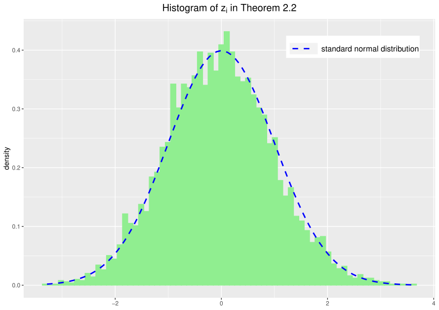
We first show the finite sample behavior of the estimator is consistent with the Central Limit Theorem of Theorem 2.1. Under the notation of Theorem 2.1, we choose $\color[rgb]{0,0,0}{\theta=0.2}$, $g(x)=x^{2}$, and estimate the functional volatility using the exponential kernel $K(x)=\frac{1}{2}e^{-|x|}$. The choice of $\theta$ was obtained from the formula $b^{*}=\theta^{*}\sqrt{\Delta_{n}}$, where $b^{*}$ was chosen using the iterative method in Figueroa-López & Li (2020). The sample frequency of the data is 1 second. Based on 5,000 simulated paths from the model (3.1), we calculate the standardized estimation error for each path $i=1,\dots,5000$ according to Theorem 2.1:

$$z_{i}=\frac{\left(\Delta_{n}\sum_{j=1}^{n}g(\hat{c}^{n,i}_{j})\bar{K}\left(t_{j}\right)-\int_{0}^{T}g(c^{i}_{s})ds\right)/\sqrt{\Delta_{n}}-(A^{1,i}+A^{2,i}+A^{3,i})}{\sqrt{{\rm Var}(Z)^{i}}},$$ (3.2)

where $c^{i}_{s}=(\sigma^{i}_{s})^{2}$, $\{\hat{c}^{n,i}_{j}\}_{j}$ are the kernel spot volatility estimates of the $i$th simulated path, and the variance ${\rm Var}(Z)^{i}=2\int_{0}^{T}(g^{\prime\prime}(c^{i}_{s})c^{i}_{s})^{2}ds$ and the biases $A^{\ell,i}$ ($\ell=1,2,3$), as defined in (2.14), are computed via Riemann sum approximations using the true simulated volatility $\{c^{n,i}_{j}\}_{j=0,\dots,n}$ and volvol observations $\{\tilde{c}^{n,i}_{j}\}_{j=0,\dots,n}$. We then compare the histogram of the standardized estimates $z_{i}$ with a standard normal distribution (see Figure 1). As shown therein, the distribution of the estimation error is consistent with the asymptotic result in Theorem 2.1.

Figure 1: Histogram of $z_{i}$ and the density of standard normal distribution in Theorem 2.1.

Similarly, we verify the behavior of the bias-corrected estimator proposed in Corollary 2.1. With the same value of $\theta$, $g(x)$, exponential kernel, and simulated data, the standardized bias-corrected estimator takes the form:

$$z_{i}=\frac{\frac{1}{\sqrt{\Delta_{n}}}\left(\widetilde{V}(g)^{n,i}_{T}-\int_{0}^{T}g(c^{i}_{s})ds\right)}{\sqrt{Var(Z^{i})}}.$$ (3.3)

The corresponding histogram is shown in Figure 2, which again suggest the CLT stated in Corollary 2.1 is valid.

Figure 2: Histogram of $z_{i}$ and the density of standard normal distribution in Corollary 2.1.

	$T=21$ days				$T=5$ days
	$\Delta_{n}=5$ minutes		$\Delta_{n}=1$ minute		$\Delta_{n}=5$ minutes		$\Delta_{n}=1$ minute
	BIAS(%)	RMSE(%)	BIAS(%)	RMSE(%)	BIAS(%)	RMSE(%)	BIAS(%)	RMSE(%)
exponential kernel
$V^{n}_{T}$	5.884	9.890	2.345	3.941	13.291	17.627	6.718	8.537
$\widetilde{V}^{n}_{T}$	1.557	8.214	0.042	3.336	1.531	16.096	0.949	6.861
two-sided uniform kernel
$V^{n}_{T}$	4.824	9.497	1.821	3.729	11.332	16.557	5.783	7.903
$\widetilde{V}^{n}_{T}$	1.804	8.357	0.084	3.352	2.288	15.843	1.183	6.874
right-sided uniform kernel
$V^{n}_{T}$	1.727	8.237	0.208	3.384	8.380	16.339	4.638	7.086
$\widetilde{V}^{n}_{T}$	1.083	8.334	-0.267	3.361	1.393	16.509	0.665	6.965
Jacod & Rosenbaum’s Estimators
$V^{n,JR}_{T}$	5.096	11.127	1.656	4.115	19.714	23.313	8.574	10.459
$\widetilde{V}^{n,JR}_{T}$	1.795	8.469	0.061	3.370	2.002	16.562	1.139	7.067
Jackknife Estimators
$TS_{n}$	4.365	8.223	2.195	3.435	3.802	14.834	2.991	6.779
$TS_{n}^{\prime}$	1.323	8.162	0.213	3.308	-8.019	20.895	-3.855	8.714
$MS_{n}$	1.989	8.220	0.098	3.347	1.618	16.641	1.041	6.930

Table 1: $g(c)=c^{2}$.

	$T=21$ days				$T=5$ days
	$\Delta_{n}=5$ minutes		$\Delta_{n}=1$ minute		$\Delta_{n}=5$ minutes		$\Delta_{n}=1$ minute
	BIAS(%)	RMSE(%)	BIAS(%)	RMSE(%)	BIAS(%)	RMSE(%)	BIAS(%)	RMSE(%)
exponential kernel
$V^{n}_{T}$	3.922	4.716	1.819	2.192	11.166	11.597	5.035	5.335
$\widetilde{V}^{n}_{T}$	0.486	2.218	0.120	0.908	1.007	4.427	0.169	2.111
two-sided uniform kernel
$V^{n}_{T}$	3.313	4.016	1.463	1.818	9.620	10.219	4.309	4.673
$\widetilde{V}^{n}_{T}$	0.300	2.790	-0.025	0.993	1.127	4.515	0.190	2.122
right-sided uniform kernel
$V^{n}_{T}$	1.224	2.373	0.485	1.045	7.605	8.281	3.379	3.800
$\widetilde{V}^{n}_{T}$	-0.753	3.440	-0.432	1.277	0.091	4.463	-0.216	2.122
Jacod & Rosenbaum’s Estimators
$V^{n,{JR}}_{T}$	4.239	4.565	1.790	2.018	17.397	17.148	7.763	7.785
$\widetilde{V}^{n,JR}_{T}$	-0.059	3.228	-0.126	1.118	0.820	4.478	0.135	2.124
Jackknife Estimators
$TS_{n}$	2.269	3.962	1.296	2.152	1.913	5.099	0.957	2.472
$TS_{n}^{\prime}$	-0.425	2.931	-0.142	1.472	-9.518	10.686	-5.169	5.547
$MS_{n}$	0.681	2.487	0.282	1.064	0.988	4.540	0.202	2.143

Table 2: $g(c)=log(c)$.

3.3 Comparison with Jackknife estimator

We now compare our bias-corrected estimator $\widetilde{V}(g)_{T}^{n}$ to the Jackknife estimator of Li et al. (2019). For the Jackknife method, we consider the two-scale estimator $TS_{n}$, its boundary-adjusted version $TS_{n}^{\prime}$, and the multiscale estimator $MS_{n}$ as defined in Li et al. (2019), Section 3.1. The parameters for the Jackknife estimators are chosen according to Li et al. (2019). By running numerous simulations, we determine that the values chosen by Li et al. (2019) broadly optimize their estimator’s performance. For the multiscale estimator $MS_{n}$, $\left(\psi_{1},\psi_{2},\psi_{3}\right)=(-2.5,8,-4.5)$, and $\left(k_{1,n},k_{2,n},k_{3,n}\right)=(15,30,45)$ for data sampled every 5 minutes, or $(40,80,120)$ for data sampled every minute. For the two-scale estimator, $\left(\psi_{1},\psi_{2}\right)=(-1,2)$ along with the same $\left(k_{1,n},k_{2,n}\right)$ as above. For our kernel estimator, we use 3 kernels: a two-sided exponential kernel $K(x)=\frac{1}{2}e^{-|x|}$, a two-sided uniform kernel $K(x)=\frac{1}{2}{\bf 1}_{[-1,1]}(x)$, and a right-sided uniform kernel $K(x)={\bf 1}_{[0,1]}(x)$. We analyze the performance of the simple biased estimator $V(g)^{n}_{T}$ in (2.9) and the bias-corrected estimator $\widetilde{V}(g)^{n}_{T}$ in (2.24). We also consider the simple biased estimator $V(g)^{n,{JR}}_{T}$ and the bias-corrected estimator $\tilde{V}(g)^{n,{JR}}_{T}$ of (2.17) and (2.26), respectively, which were proposed in Jacod & Rosenbaum (2015).

The bandwidths of all the kernel estimators are chosen using the iterative method in Figueroa-López & Li (2020), Section 5. We iterate the method only once. For a two-sided kernel, the integrated volatility of volatility used when updating the bandwidth is estimated by the Two-time Scale Realized Volatility (TSRV) estimator proposed in Figueroa-López & Li (2020). For the right-sided uniform kernel, the TSRV estimator no longer applies. We then use the realized variance estimator on the estimated volatility path as a replacement. As finite-sample corrections, in (2.24), at each $t_{i}$, we replace $\int_{-\infty}^{\infty}K^{2}(u)du$ with $\sum_{j=1}^{n}K^{2}_{h}(t_{i}-t_{j})\Delta_{n}h$, and replace $\int_{-\infty}^{\infty}L(s)ds$ and $\int_{-\infty}^{\infty}L^{2}(s)ds$ with $\frac{\Delta_{n}}{b}\sum_{j=1}^{n}L\left(\frac{t_{j-1}-t_{i}}{b}\right)$ and $\frac{\Delta_{n}}{b}\sum_{j=1}^{n}L^{2}\left(\frac{t_{j}-t_{i}}{b}\right)$, respectively, where $L\left(\frac{t_{j}-t_{i}}{b}\right)=-\sum_{l=1}^{j}K_{{b}}(t_{l-1}-t_{i})$ if $j\leq i$ and $\sum_{l=j+1}^{n}K_{{b}}(t_{l-1}-t_{i})$ if $j>i$.

In Table 1, we report the relative bias and relative root-mean-square-errors in percentage unit for the considered estimators. Our results of the Jackknife estimators are consistent with the ones in Li et al. (2019), Table 1 therein. As shown in Table 1, the kernel estimators exhibit a similar performance to the Jackknife estimators. However, the Jackknife estimators have more tuning parameters, while ours requires only one tuning parameter (namely, $\theta$). As we will show in Section 3.3.1, the fundamental advantage of our estimators lie on their stability relative to the choice of the bandwidth. That is, our estimators seem to exhibit satisfactory performance for a large range of the tuning parameters, while other estimators are more sensitive to choosing ‘good’ values for their tuning parameters.

Returning to the results of Table 1, we also observe that in some cases the kernel estimators have smaller relative root mean square error (RMSE) compared with the Jackknife estimators, especially when the time span $T$ is short ($T=5$ days). Intuitively, the superior performance of the spot volatility estimators with exponential kernel (shown in Figueroa-López & Li (2020), Section 7) is expected to be more evident when the time span is relatively short, e.g. 5 days. For reference, we include the tables for the function $g(c)=log(c)$ in Table 2. These tables confirm our previous conclusion. It is worth noting that in general, the bias-corrected kernel estimator $\widetilde{V}^{n}_{T}$ has significantly smaller RMSE compared with the simple biased estimator $V(g)^{n}_{T}$, which also happens among the Jacod & Rosenbaum’s estimators, $V(g)^{n,{JR}}_{T}$ and $\widetilde{V}^{n,JR}_{T}$.

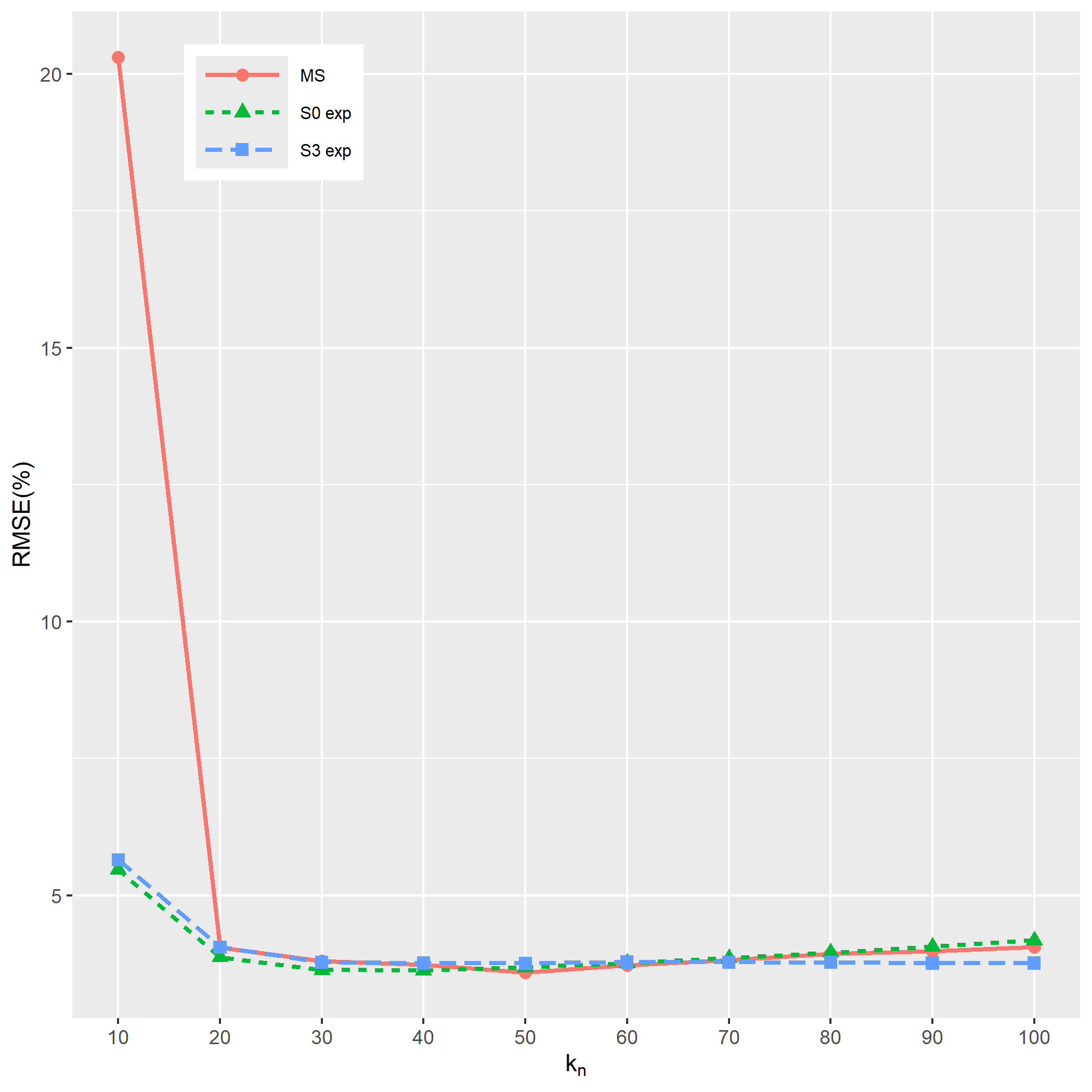
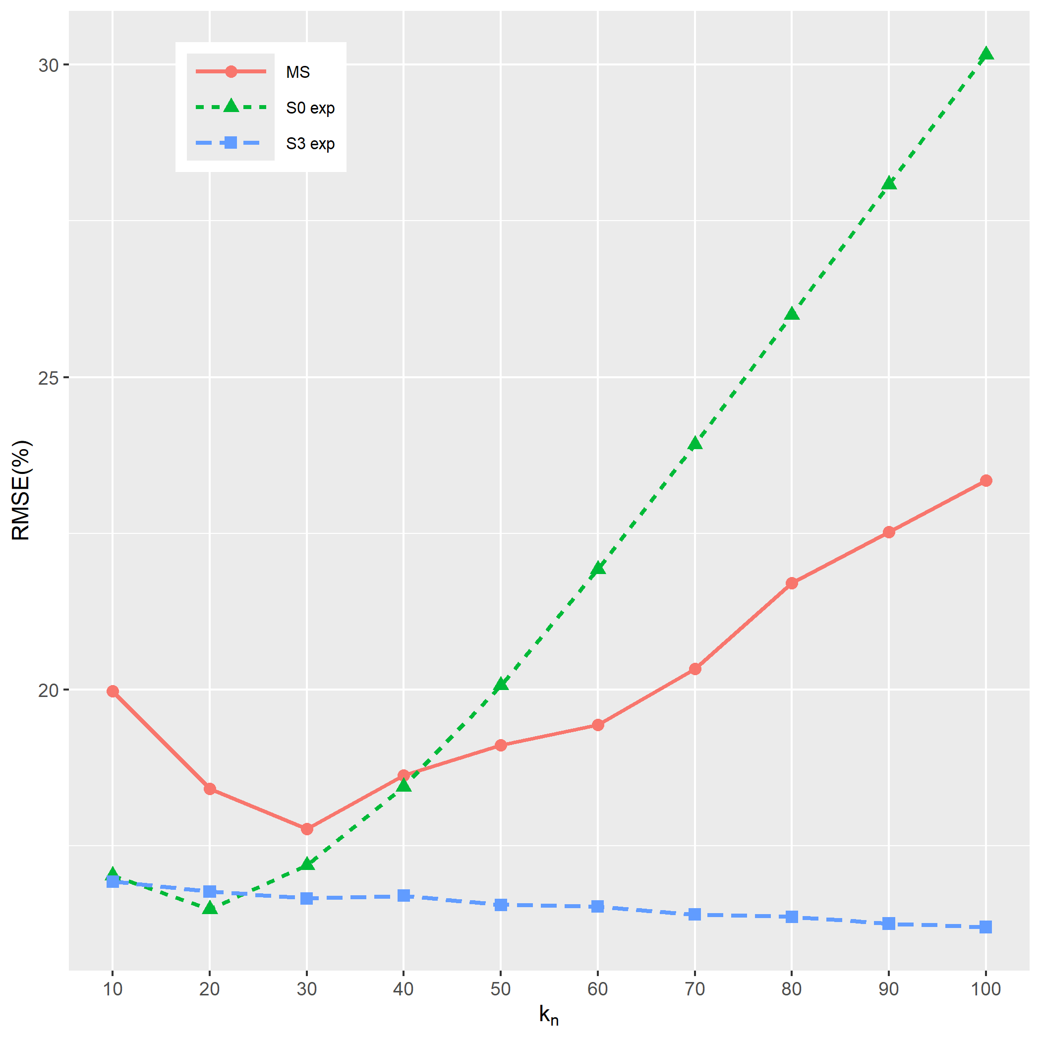
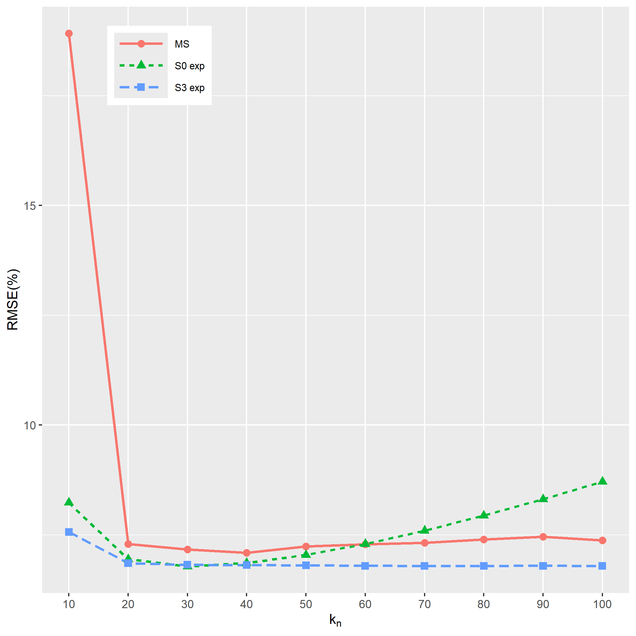
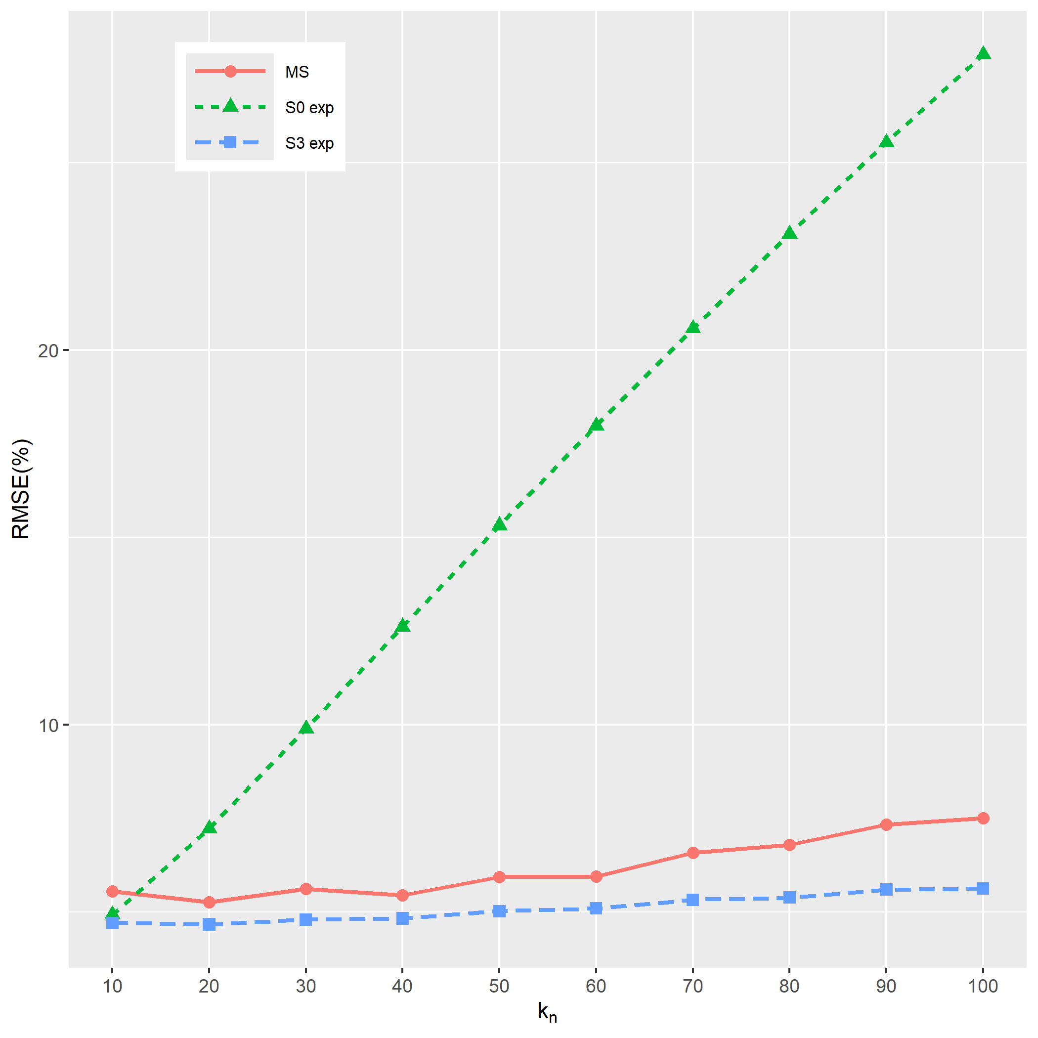
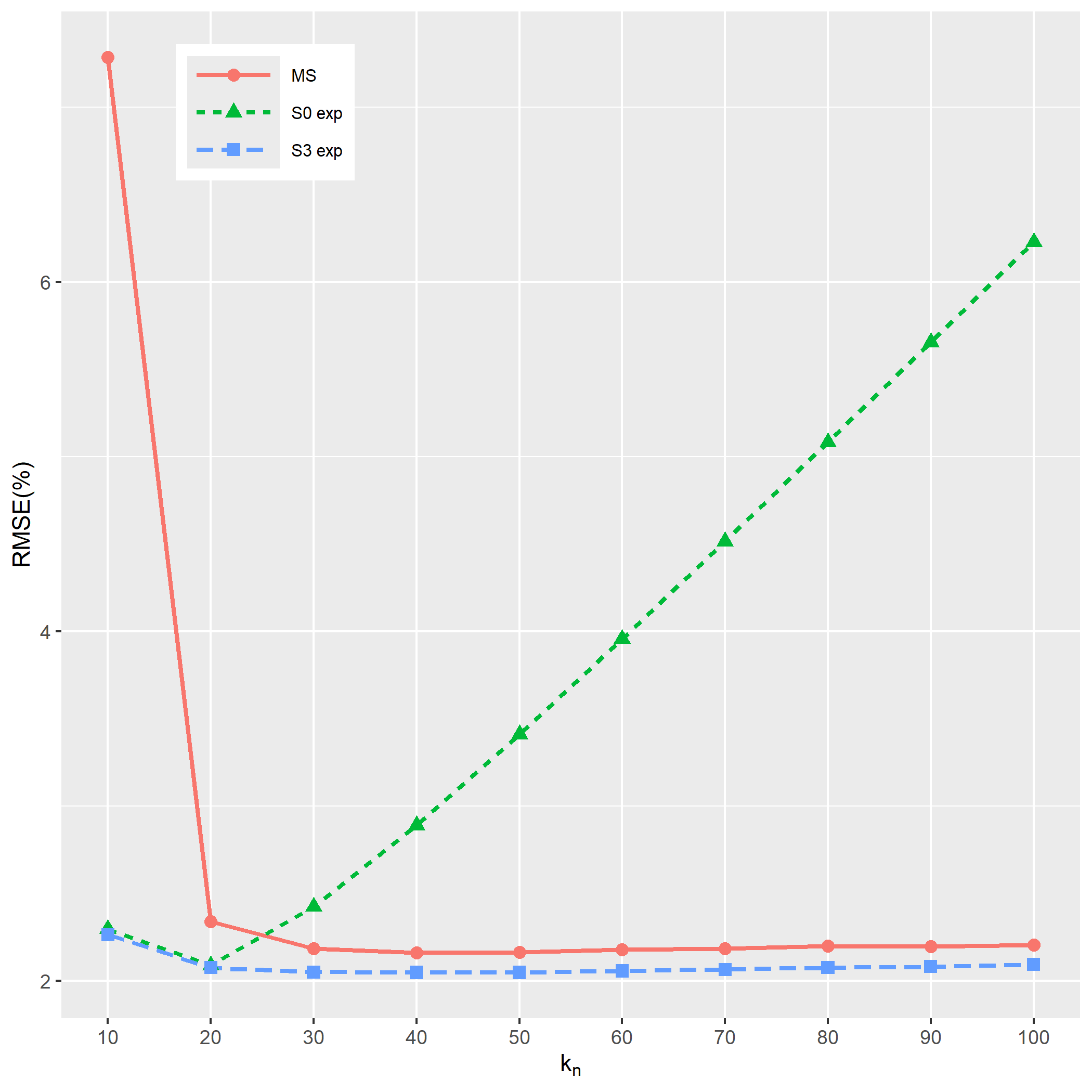
3.3.1 Bandwidth Sensitivity

In this subsection, we investigate how sensitive the estimators are relative to the bandwidth parameter. For the Jackknife estimators, we focus on the boundary adjusted multi-scale estimator MS (which, as shown in Tables 1 and 2, typically has the best performance among all Jackknife estimators), and for the kernel estimators, we first consider an exponential kernel. We try a sequence of bandwidths $k_{n}$ for the kernel estimator, and a sequence of triplets $(k_{1,n},k_{2,n},k_{3,n})=([\frac{k_{n}}{2}],k_{n},[\frac{3k_{n}}{2}])$ and $(\psi_{1},\psi_{2},\psi_{3})=(-2.5,8,-4.5)$ for $MS$, which include the parameters chosen in Li et al. (2019) when $k_{n}=30$ (see Table 1 therein). The results are shown in the Figures 3-6, where S0 exp denotes the simple biased exponential kernel estimator in (2.9) and S3 exp denotes the bias-corrected estimators with exponential kernel in (2.24). We can conclude that the estimator S3 exp exhibits the most stable or consistent performance for either 5 or 21 days data with 1 or 5 minutes sampling frequency, and both $g(c)=c^{2}$ or $\log(c)$. In other words, the estimator’s values are in general relatively invariant to changes in the bandwidth, especially when working with low frequency and $g(c)=c^{2}$. Under those conditions, the others estimators require more careful tuning of the bandwidth in order to show good performance. We can also observe that the bias-corrected exponential kernel estimator almost always outperforms the boundary-adjusted multi-scale Jackknife estimator MS and the simple biased exponential kernel estimator S0 exp.

Finally, in Figure 7, we analyze the bandwidth stability of three estimators: the bias-corrected estimators (2.24) with exponential and right-sided uniform kernels and the bias-corrected estimator (2.26) proposed in Jacod & Rosenbaum (2015). Again, since we are not introducing jumps in the process $X$, the estimator $\hat{c}_{i}^{n}$ used for (2.24) and the estimator $\hat{c}_{i}^{n,{JR}}$ used for (2.26) do not have any truncation (i.e., we fix $v_{n}=\infty$ in (2.5) and (2.16)). Figure 7 shows that our proposed estimator $\widetilde{V}^{n}_{T}$ with either exponential or right-sided uniform kernel almost always outperforms $\widetilde{V}^{n,JR}_{T}$. The exponential kernel appears to be less sensitive to the choice of $k_{n}$ than the right-sided uniform kernel. The estimator $\widetilde{V}^{n,JR}_{T}$ also seems to require a careful tuning of the bandwidth in order to achieve a good performance.

(a) data with 5 minute sample frequency.

(b) data with 1 minute sample frequency.

Figure 3: RMSE(%) v.s. the bandwidth $k_{n}$, for 21 days data, $g(c)=c^{2}$ and 1000 simulated path. $S0$ exp denotes the simple biased estimator with exponential kernel and $S3$ exp denotes the unbiased estimator with exponential kernel.

(a) data with 5 minute sample frequency.

(b) data with 1 minute sample frequency.

Figure 4: RMSE(%) v.s. the bandwidth $k_{n}$, for 5 days data, $g(c)=c^{2}$ and 1000 simulated path. $S0$ exp denotes the simple biased estimator with exponential kernel and $S3$ exp denotes the unbiased estimator with exponential kernel.

(a) data with 5 minute sample frequency.

(b) data with 1 minute sample frequency.

Figure 5: RMSE(%) v.s. the bandwidth $k_{n}$, for 21 days data, $g(c)=log(c)$ and 1000 simulated path. $S0$ exp denotes the simple biased estimator with exponential kernel and $S3$ exp denotes the unbiased estimator with exponential kernel.

(a) data with 5 minute sample frequency.

(b) data with 1 minute sample frequency.

Figure 6: RMSE(%) v.s. the bandwidth $k_{n}$, for 5 days data, $g(c)=log(c)$ and 1000 simulated path. $S0$ exp denotes the simple biased estimator with exponential kernel and $S3$ exp denotes the unbiased estimator with exponential kernel.

(a) data with 5 minute sample frequency.

(b) data with 1 minute sample frequency.

Figure 7: RMSE(%) v.s. the bandwidth $k_{n}$, for 5 days data, $g(c)=c^{2}$ and 1000 simulated path. $S3$ exp and $S3$ unif denotes the unbiased estimator with exponential kernel and right-sided uniform kernel, respectively. $S3$ JR corresponds to the bias-corrected estimator (2.26) in Jacod & Rosenbaum (2015).

Appendix A Proof of Main Results

By virtue of localization, without loss of generality, we assume throughout the proof that, for some constant $A$,

$$\Gamma(z)+\int\Gamma(z)^{r}\lambda(dz)+\left|\mu_{t}\right|+\left|\sigma_{t}\right|+\left|X_{t}\right|+\left|\mu_{t}^{\prime}\right|+\left|\tilde{\sigma}_{t}\right|+\left|\tilde{\mu}_{t}\right|\leq A,\text{ for any }t\leq T,$$ (A.1)

(see Section 4.4.1 and (6.2.1) in Jacod & Protter (2011) and Appendix A.5 in Aït-Sahalia & Jacod (2014) for details).

We use $C$ to represent a generic constant that may change from line to line. We first need some notations:

$$\begin{split}\alpha_{i}^{n}&:=\left(\Delta_{i}^{n}X^{\prime}\right)\left(\Delta_{i}^{n}X^{\prime}\right)^{*}-c_{i-1}^{n}\Delta_{n}\in\mathbb{R}^{d\times d},\\ \beta_{i}^{n}:=\hat{c}_{i}^{\prime n}-c_{i}^{n}&=\frac{\sum_{j=1}^{n}K_{{k}_{n}\Delta_{n}}\left(t_{j-1}-t_{i}\right)\left(\Delta_{j}^{n}X^{\prime}\right)\left(\Delta_{j}^{n}X^{\prime}\right)^{*}}{\Delta_{n}\sum_{j=1}^{n}K_{{k}_{n}\Delta_{n}}\left(t_{j-1}-t_{i}\right)}-c_{i}^{n}\\ &=\frac{1}{\bar{K}\left(t_{i}\right)}\sum_{j=1}^{n}K_{{b}}\left(t_{j-1}-t_{i}\right)\left[\alpha_{j}^{n}+\left(c_{j-1}^{n}-c_{i}^{n}\right)\Delta_{n}\right],\end{split}$$ (A.2)

and $\tilde{\beta}_{i}^{n}:=\beta_{i}^{n}\bar{K}\left(t_{i}\right)$. The nice decomposition of the estimation error $\beta_{i}^{n}=\hat{c}_{i}^{\prime n}-c_{i}^{n}$ in terms of the $\alpha_{j}^{n}$ and $c_{j-1}^{n}-c_{i}$ was possible because of the denominator $\bar{K}(t_{i})$ in the estimator $\hat{c}_{i}^{\prime n}$ and this is one of the reasons why this was added. For an uniform kernel, $\bar{K}(t_{i})$ equal to $1$ for almost all $i$ and is not needed if one considers the truncated version (1.2) as in Jacod & Rosenbaum (2013). However, it seems more natural to include the “standardized” term $\bar{K}(t_{i})$.

For any process $Z$, we set:

$$\begin{split}\eta(Z)_{t,s}&=\sqrt{\mathbb{E}\left(\sup_{v\in(t,t+s]}\left\|Z_{{\color[rgb]{0,0,0}v}}-Z_{t}\right\|^{2}\Big{|}\mathcal{F}_{t}\right)},\\ \eta(Z)^{n}_{i,j}&=\eta\left(Z\right)_{i\Delta_{n},j\Delta_{n}},\\ \eta(Z)^{n}_{i-1}&=\eta(Z)^{n}_{(i-1),1}.\end{split}$$ (A.3)

By Lemma 16.5.15 in Jacod & Protter (2011), if $U$ is a càdlàg bounded process, we have for all $q>0$,

$$\Delta_{n}\mathbb{E}\left(\sum_{i=1}^{\left[t/\Delta_{n}\right]}\left|\eta(U)^{n}_{i-1}\right|^{q}\right)\rightarrow 0.$$ (A.4)

For future reference, we hereafter denote the continuous version of the process (2.1) as

$$X^{\prime}_{t}:=X_{0}+\int_{0}^{t}\mu^{\prime}_{s}ds+\int_{0}^{t}\sigma_{s}dW_{s},$$ (A.5)

where $\mu_{t}^{\prime}=\mu_{t}-\int_{\{z:\|\delta(t,z)\|\leq 1\}}\delta(t,z)\lambda(dz)$. We also let $\hat{c}_{i}^{\prime n}:=\hat{c}_{i}^{n,X^{\prime}}$ be the Nadaraya-Watson kernel estimator (2.3) based on the continuous process $X^{\prime}$ defined in (A.5). Finally, we define the estimators of the integrated volatility functionals based on the continuous process as:

$${\color[rgb]{0,0,0}V(g)_{t}^{\prime n}:=\Delta_{n}\sum_{i=1}^{\left[t/\Delta_{n}\right]}g\left(\hat{c}_{i}^{\prime n}\right)\bar{K}\left(t_{i}\right)}.$$ (A.6)

A.1 Preliminary Result

Let us recall the following estimates:

1. By (3.10) in Jacod & Rosenbaum (2015), under (A.1), for any $s,t\geq 0$ and $q\geq 0$ :

   $$\begin{array}[]{ll}{\rm(i)}\;\mathbb{E}\left(\sup_{w\in[0,s]}\left\|X^{\prime}_{t+w}-X^{\prime}_{t}\right\|^{q}\mid\mathcal{F}_{t}\right)\leq C_{q}s^{q/2},&{\rm(ii)}\;\left\|\mathbb{E}\left(X^{\prime}_{t+s}-X^{\prime}_{t}\mid\mathcal{F}_{t}\right)\right\|\leq Cs,\\ {\rm(iii)}\;\mathbb{E}\left(\sup_{w\in[0,s]}\left\|c_{t+w}-c_{t}\right\|^{q}\mid\mathcal{F}_{t}\right)\leq C_{q}s^{1\wedge(q/2)},&{\rm(iv)}\;\left\|\mathbb{E}\left(c_{t+s}-c_{t}\mid\mathcal{F}_{t}\right)\right\|\leq Cs,\end{array}$$ (A.7)

   where recall that above $\|x\|$ is the Euclidian norm of a $d\times d$-matrix $x$, considered as a $\mathbb{R}^{d\times d}$ vector.

2. From Jacod & Rosenbaum (2015) (3.20) and (3.24), or BDG and Hölder inequalities. We have

   $$\begin{array}[]{l}{\rm(i)}\;\mathbb{E}\left(\left\|\alpha_{i}^{n}\right\|^{q}\mid\mathcal{F}_{i-1}^{n}\right)\leq C_{q}\Delta_{n}^{q},\quad{\rm(ii)}\;\left\|\mathbb{E}\left(\alpha_{i}^{n}\mid\mathcal{F}_{i-1}^{n}\right)\right\|\leq C\Delta_{n}^{3/2},\quad{\rm(iii)}\;\mathbb{E}\left(\left\|\hat{c}_{i}^{\prime n}\right\|^{q}\mid\mathcal{F}_{i-1}^{n}\right)\leq C_{q}.\end{array}$$ (A.8)

3. From (3.22) and (3.24) in Jacod & Rosenbaum (2015) and notation (A.3), we have

   $$\begin{array}[]{l}\left|\mathbb{E}\left(\alpha_{i}^{n,\ell m}\mid\mathcal{F}_{i-1}^{n}\right)\right|\leq C\Delta_{n}^{3/2}\left(\sqrt{\Delta_{n}}+\eta_{i-1}^{n}\right)\\ \left|\mathbb{E}\left(\alpha_{i}^{n,jk}\alpha_{i}^{n,lm}\mid\mathcal{F}_{i-1}^{n}\right)-\left(c_{i-1}^{n,jl}c_{i-1}^{n,km}+c_{i-1}^{n,jm}c_{i-1}^{n,kl}\right)\Delta_{n}^{2}\right|\leq C\Delta_{n}^{5/2}\\ \left|\mathbb{E}\left(\alpha_{i}^{n,jk}\Delta_{i}^{n}c^{lm}\mid\mathcal{F}_{i-1}^{n}\right)\right|\leq C\Delta_{n}^{3/2}\left(\sqrt{\Delta_{n}}+\eta_{i-1}^{n}\right)\\ \left|\mathbb{E}\left(\alpha_{i}^{n,jk}\Delta_{i}^{n}W^{l}\mid\mathcal{F}_{i-1}^{n}\right)\right|\leq C\Delta_{n}^{3/2}\left(\sqrt{\Delta_{n}}+\eta_{i-1}^{n}\right),\end{array}$$ (A.9)

   where

   $$\eta_{i-1}^{n}=\max\left(\eta\left(Y\right)^{n}_{i-1}:Y=\mu,\widetilde{\mu},c,\tilde{c},\widehat{c}\right).$$ (A.10)

4. By (A.8) and (A.9), we have for $q\geq 2,$

   $$\mathbb{E}\left[\left\|\beta^{n}_{i}\right\|^{q}\right]={\mathbb{E}\left[\left\|\hat{c}_{i}^{\prime n}-c_{i}^{n}\right\|^{q}\right]}\leq C_{q}\left(k_{n}^{-q/2}+(k_{n}\Delta_{n})^{q/2}\right).$$ (A.11)

   The proof is included in Appendix B.1 for completeness.

5. We shall use often the following asymptotic approximation:

   $$\Delta_{n}\sum_{i=1}^{n}K_{{b}}\left(t_{i-1}-\tau\right)=\int K(u)du+O(\Delta_{n}/{b})=1+O(\Delta_{n}/{b}),$$ (A.12)

   where the error is uniform on $\tau\in{\color[rgb]{0,0,0}B}$, for any compact set ${\color[rgb]{0,0,0}B}\subseteq(0,T)$. Furthermore, we can show that there exists $\delta>0$ such that for any $n$ and $t_{i}$,

   $$\delta<\left|\bar{K}_{n}\left(t_{i}\right)\right|=\left|\Delta_{n}\sum_{j=1}^{n}K_{{k}_{n}\Delta_{n}}\left(t_{j-1}-t_{i}\right)\right|<\frac{1}{\delta}.$$ (A.13)

   The proofs of (A.12) and (A.13) are given in Appendix B.1.

The following result will be used several times. Its proof is similar to that of Lemma 3.1 in Figueroa-López & Li (2020) and is given in Appendix B.1 for completeness.

Lemma A.1.

Let $f:\mathcal{M}_{d}^{+}\rightarrow\mathbb{R}$ and $K:\mathbb{R}\rightarrow\mathbb{R}$ be such that

1. $f$ is $C^{1}$ and $|f(x)|\leq C(1+\|x\|^{p})$ for some $p\geq 3$;

2. $K$ is absolutely continuous and $K^{\prime}$ exists piecewise on $(A,B)$ (in particular, recall that its support is $(A,B)$ for some $A<B$ such that $A\in[-\infty,0]$ and $B\in[0,\infty]$); $\int\left|K(x)\right|dx<\infty$; $\int\left|K^{\prime}(x)\right|dx<\infty$; $V_{-\infty}^{\infty}(K^{\prime})<\infty$.

Suppose also that $\Delta_{n},b_{n}\to 0$ such that $\Delta_{n}/{b}_{n}\to{}0$. Then, the following assertions hold true:

1. Let

   $$D_{1}(f):=\sum_{i=1}^{n}K_{{b}}\left(t_{i-1}-\tau\right)\int_{t_{i-1}}^{t_{i}}f\left(c_{s}\right)ds-\int_{0}^{T}K_{{b}}\left(s-\tau\right)f\left(c_{s}\right)ds.$$

   Then, for each $\tau\in(0,T)$,

   $$D_{1}(f)=\frac{1}{2}f(c_{\tau})\left(K\left(A^{+}\right)-K\left(B^{-}\right)\right)\frac{\Delta_{n}}{b}+o\left(\frac{\Delta_{n}}{b}\right).$$ (A.14)

   Furthermore, for $\tau=0$ or $T$, we have $D_{1}(f)=O_{p}\left(\frac{\Delta_{n}}{b}\right)$.

2. Let

   $$D_{2}(f):=\sum_{i=1}^{n}K_{{b}}\left(t_{i-1}-\tau\right)f\left(c_{i}^{n}\right)\Delta_{n}-\int_{0}^{T}K_{{b}}\left(s-\tau\right)f\left(c_{s}\right)ds.$$

   Then, for each $\tau\in[0,T]$,

   $$D_{2}(f)=D_{1}(f)+O_{p}(\Delta_{n}^{1/2}).$$ (A.15)

Remark A.1.

In Lemma A.1-(i), $\tau$ is a constant time in $(0,T)$. However, in the definition of our estimator (2.5) and in some of the proofs below, we need to take $\tau=t_{j}$ for some $j=0,\dots,n$. In that case, following the same proof as that of Lemma A.1-(i), one can show that for a constant $C\in(0,\infty)$,

$$\limsup_{n\to\infty}\frac{b_{n}}{\Delta_{n}}|D_{1}(f)|\leq C|f(c_{\tau})|.$$

A.2 Proof of Theorem 2.1

A.2.1 Elimination of the jumps and the truncation

Lemma A.2.

Under (2.1), (2.10), and Assumptions 1 & 2, the following assertions hold:

• For any $q\geq 1$, $q^{\prime}>0$, and a sequence $a_{n}$ going to 0, we have:

  $$\mathbb{E}\left[\left\|\hat{c}_{i}^{n}-\hat{c}_{i}^{\prime n}\right\|^{q}\right]\leq Ca_{n}\Delta_{n}^{(2q-r)\varpi+1-q}+C\Delta_{n}^{q^{\prime}(1-2\varpi)},$$ (A.16)

  where $\hat{c}$ is defined as in (2.5) with $v_{n}=\alpha\Delta_{n}^{\varpi}$ and $0<\varpi<1/2$, and $\hat{c}_{i}^{\prime n}:=\hat{c}_{i}^{n,X^{\prime}}$ is the Nadaraya-Watson kernel estimator (2.3) based on the continuous process $X^{\prime}$ defined in (A.5). Based on (A.16), under the condition (2.7), we have the following:

  $$\frac{1}{\sqrt{\Delta_{n}}}\left[V(g)_{T}^{n}-V(g)_{T}^{\prime n}\right]\xrightarrow{\mathbb{P}}0,$$ (A.17)

  where recall that $V(g)_{T}^{\prime n}$ is defined as in (A.6).

• Furthermore, if $X$ is continuous (i.e., $\delta\equiv 0$ in (2.1)), then for any $q^{\prime}>0$, (A.16) becomes

  $$\mathbb{E}\left[\left\|\hat{c}_{i}^{n}-\hat{c}_{i}^{\prime n}\right\|^{q}\right]\leq C\Delta_{n}^{q^{\prime}(1-2\varpi)},$$ (A.18)

  based on which, under (2.6), (A.17) holds true as well.

Proof.

We consider the case of discontinuous $X$ first. By Minkowski’s and Jensen’s inequality, for any $q\geq 1$,

$$\mathbb{E}\left[\left\|\hat{c}_{i}^{n}-\hat{c}_{i}^{\prime n}\right\|^{q}\right]$$

$$=\mathbb{E}\left[\left\|\bar{K}_{n}\left(t_{i}\right)^{-1}\sum_{j=1}^{n}K_{k_{n}\Delta_{n}}\left(t_{j-1}-t_{i}\right)\left[\left(\Delta_{j}X\right)\left(\Delta_{j}X\right)^{*}\mathbbm{1}_{\left\{\left\|\Delta_{j}X\right\|\leq v_{n}\right\}}-\left(\Delta_{j}X^{\prime}\right)\left(\Delta_{j}X^{\prime}\right)^{*}\right]\right\|^{q}\right]$$

$$\leq C_{q}\mathbb{E}\left[\left\|\sum_{j=1}^{n}K_{k_{n}\Delta_{n}}\left(t_{j-1}-t_{i}\right)\left(\Delta_{j}X^{\prime}\right)\left(\Delta_{j}X^{\prime}\right)^{*}\mathbbm{1}_{\left\{\left\|\Delta_{j}X^{\prime}\right\|>v_{n}\right\}}\right\|^{q}\right]$$

$$+C_{q}\mathbb{E}\left[\left\|\sum_{j=1}^{n}K_{k_{n}\Delta_{n}}\left(t_{j-1}-t_{i}\right)\left[\left(\Delta_{j}X\right)\left(\Delta_{j}X\right)^{*}\mathbbm{1}_{\left\{\left\|\Delta_{j}X\right\|\leq v_{n}\right\}}-\left(\Delta_{j}X^{\prime}\right)\left(\Delta_{j}X^{\prime}\right)^{*}\mathbbm{1}_{\left\{\left\|\Delta_{j}X^{\prime}\right\|\leq v_{n}\right\}}\right]\right\|^{q}\right]$$

$$\leq C_{q}\left[\sum_{j=1}^{n}\left|K_{k_{n}\Delta_{n}}\left(t_{j-1}-t_{i-1}\right)\right|\right]^{q-1}\sum_{j=1}^{n}\left|K_{k_{n}\Delta_{n}}\left(t_{j-1}-t_{i-1}\right)\right|\mathbb{E}\left[\left\|\left(\Delta_{j}X^{\prime}\right)\right\|^{2q}\mathbbm{1}_{\left\{\left\|\Delta_{j}X^{\prime}\right\|>v_{n}\right\}}\right]$$

$$+C_{q}\left[\sum_{j=1}^{n}\left|K_{k_{n}\Delta_{n}}\left(t_{j-1}-t_{i-1}\right)\right|\right]^{q-1}\sum_{j=1}^{n}\left|K_{k_{n}\Delta_{n}}\left(t_{j-1}-t_{i-1}\right)\right|$$

$$\quad\quad\quad\quad\quad\quad\quad\quad\quad\quad\quad\quad\mathbb{E}\left[\left\|\left(\Delta_{j}X\right)\left(\Delta_{j}X\right)^{*}\mathbbm{1}_{\left\{\left\|\Delta_{j}X\right\|\leq v_{n}\right\}}-\left(\Delta_{j}X^{\prime}\right)\left(\Delta_{j}X^{\prime}\right)^{*}\mathbbm{1}_{\left\{\left\|\Delta_{j}X^{\prime}\right\|\leq v_{n}\right\}}\right\|^{q}\right].$$

Furthermore, we have

$$\mathbb{E}\left[\left\|\left(\Delta_{j}X^{\prime}\right)\right\|^{2q}\mathbbm{1}_{\left\{\left\|\Delta_{j}X^{\prime}\right\|>v_{n}\right\}}\right]\leq\left\{\mathbb{E}\left[\left\|\left(\Delta_{j}X^{\prime}\right)\right\|^{4q}\right]\right\}^{1/2}\left\{\mathbb{E}\left[\mathbbm{1}_{\left\{\left\|\Delta_{j}X^{\prime}\right\|>v_{n}\right\}}\right]\right\}^{1/2},$$

where, by Markov’s inequality and (A.7),

$$\mathbb{E}\left[\mathbbm{1}_{\left\{\left\|\Delta_{j}X^{\prime}\right\|>v_{n}\right\}}\right]\leq\frac{\mathbb{E}\left[\left\|\left(\Delta_{j}X^{\prime}\right)\right\|^{4q^{\prime}}\right]}{v_{n}^{4q^{\prime}}}\leq\frac{K_{q}\Delta_{n}^{2q^{\prime}}}{\Delta_{n}^{4q^{\prime}\varpi}},$$

for any $q^{\prime}>0$ by Markov inequality. Thus,

$$\mathbb{E}\left[\left\|\left(\Delta_{j}X^{\prime}\right)\right\|^{2q}\mathbbm{1}_{\left\{\left\|\Delta_{j}X^{\prime}\right\|>v_{n}\right\}}\right]\leq C\Delta_{n}^{q+q^{\prime}(1-2\varpi)}.$$

Meanwhile, by Lemma 13.2.6 of Jacod & Protter (2011), with $F(x)=xx^{*},m=q,p^{\prime}=s^{\prime}=2,s=1,k=1,j=0$, we have for some sequence $a_{n}$ going to 0,

$$\mathbb{E}\left(\left\|\left(\Delta_{i}^{n}X\right)\left(\Delta_{i}^{n}X^{*}\right)\mathbbm{1}_{\left\{\left\|\Delta_{i}^{n}X\right\|\leq v_{n}\right\}}-\left(\Delta_{i}^{n}X^{\prime}\right)\left(\Delta_{i}^{n}X^{\prime*}\right)\mathbbm{1}_{\left\{\left\|\Delta_{i}^{n}X^{\prime}\right\|\leq v_{n}\right\}}\right\|^{q}\right)\leq Ca_{n}\Delta_{n}^{(2q-r)\varpi+1},$$ (A.19)

where, from Assumption 1, $r<1$. Hence, the difference between $\hat{c}_{i}^{n}$ and $\hat{c}_{i}^{\prime n}$ can be estimated by

$$\mathbb{E}\left[\left\|\hat{c}_{i}^{n}-\hat{c}_{i}^{\prime n}\right\|^{q}\right]\leq Ca_{n}\Delta_{n}^{(2q-r)\varpi+1-q}+C\Delta_{n}^{q^{\prime}(1-2\varpi)},$$

and (A.16) is proved. Note that

$$V(g)_{T}^{n}-V(g)_{T}^{\prime n}=\Delta\sum_{i=1}^{n}\left[g\left(\hat{c}_{i}^{n}\right)-g\left(\hat{c}_{i}^{\prime n}\right)\right]\bar{K}\left(t_{i}\right),$$

and, by (2.10) and the mean value theorem, for some $\xi\in[0,1]$,

$$\left|g\left(\hat{c}_{i}^{n}\right)-g\left(\hat{c}_{i}^{\prime n}\right)\right|\leq\left\|\nabla g\left(\xi\hat{c}_{i}^{n}+\left(1-\xi\right)\hat{c}_{i}^{\prime n}\right)\right\|\left\|\hat{c}_{i}^{n}-\hat{c}_{i}^{\prime n}\right\|$$ (A.20)

$$\leq C\left(1+\left\|\xi\hat{c}_{i}^{n}+\left(1-\xi\right)\hat{c}_{i}^{\prime n}\right\|^{p-1}\right)\left\|\hat{c}_{i}^{n}-\hat{c}_{i}^{\prime n}\right\|.$$

By (A.16), if we let $q=1$ and $q^{\prime}>\frac{1}{1-2\varpi}$, since $\varpi\in\left[\frac{2p-1}{2(2p-r)},\frac{1}{2}\right)$, we have

$$\mathbb{E}\left[\left\|\hat{c}_{i}^{n}-\hat{c}_{i}^{\prime n}\right\|\right]\leq Ca_{n}\Delta_{n}^{\frac{(2-r)(2p-1)}{2(2p-r)}}+C\Delta_{n},$$

which converges to zero at the rate of $o(\sqrt{\Delta_{n}})$ . Plug it back in (A.20), we have

$$\mathbb{E}\left[\left|g\left(\hat{c}_{i}^{n}\right)-g\left(\hat{c}_{i}^{\prime n}\right)\right|\right]=o(\sqrt{\Delta_{n}}),$$ (A.21)

and (A.17) is obtained.

We now proceed to show (b). In that case, $X$ is continuous (i.e., $X=X^{\prime}$) and clearly the $q$th moment in (A.19) is zero. Thus, (A.16) simplifies as (A.18). Let $q^{\prime}>\frac{1}{1-2\varpi}$ and (A.17) follows by (A.20), (A.18), and (2.6). ∎

With Lemma A.2 and the previous arguments, it remains to prove Theorem 2.1 in the continuous case with $\hat{c}$ as (2.3) under the following assumption:

Assumption 3.

We have (2.1) with $X$ continuous, $c_{t}:=\sigma_{t}\sigma_{t}^{*}$ satisfies (2.2), the processes $\mu,\tilde{\mu},\sigma,\tilde{\sigma}$ are bounded.

We shall exploit the following decomposition

$$\frac{1}{\sqrt{\Delta_{n}}}\left(V(g)_{T}^{n}-V(g)_{T}\right)=\sum_{j=1}^{5}V^{n}_{j},$$ (A.22)

where

$$\begin{array}[]{l}V^{n}_{1}=\frac{1}{\sqrt{\Delta_{n}}}\sum_{i=1}^{n}\int_{t_{i-1}}^{t_{i}}\left(g\left(c_{i}^{n}\right)-g\left(c_{s}\right)\right)ds,\\ V^{n}_{2}=\sqrt{\Delta_{n}}\sum_{i=1}^{n}\sum_{j=1}^{n}K_{{b}}\left(t_{j-1}-t_{i}\right)\nabla g\left(c_{i}^{n}\right)\cdot\alpha_{j}^{n},\\ V^{n}_{3}=\sqrt{\Delta_{n}}\sum_{i=1}^{n}\sum_{j=1}^{n}K_{{b}}\left(t_{j-1}-t_{i}\right)\nabla g\left(c_{i}^{n}\right)\cdot\left(c_{j-1}^{n}-c_{i}^{n}\right)\Delta_{n},\\ V^{n}_{4}=\sqrt{\Delta_{n}}\sum_{i=1}^{n}\left[(g\left(c_{i}^{n}+\beta_{i}^{n}\right)-g\left(c_{i}^{n}\right)-\nabla g(c_{i}^{n})\cdot\beta_{i}^{n}\right]{\color[rgb]{0,0,0}\bar{K}_{n}\left(t_{i}\right)},\\ V^{n}_{5}=\sqrt{\Delta_{n}}\sum_{i=1}^{n}\left[\bar{K}_{n}\left(t_{i}\right)-1\right]g\left(c_{i}^{n}\right).\end{array}$$ (A.23)

Above, recall that $x\cdot y=\sum_{\ell,m}x^{\ell m}y^{\ell m}$ for $x,y\in\mathbb{R}^{d\times d}$ (thus, e.g., $\nabla g(c_{i}^{n})\cdot\beta_{i}^{n}:=\sum_{\ell,m}\partial_{\ell m}g(c_{i}^{n})\beta_{i}^{n,\ell m}$).

The first term $V^{n}_{1}$ converge to 0 since $g$ is $C^{2}$ and $c_{t}$ is an Itô semimartingale with bounded characteristics (see, e.g., (5.3.24) in Jacod & Protter (2011)). In the subsequence subsections, we show the convergence for each of the other terms in the decomposition.

A.2.2 The leading term $V^{n}_{2}$

In this section, we show

$$V^{n}_{2}\stackrel{{\scriptstyle st}}{{\Longrightarrow}}Z,$$ (A.24)

where $Z$ is defined as in the statement of Theorem 2.1. Denoting $w_{j}=\Delta_{n}\sum_{i=1}^{n}K_{{b}}(t_{j-1}-t_{i})\nabla g(c^{n}_{i})\in\mathbb{R}^{d\times d}$, we can rewrite $V^{n}_{2}$ as

$$\begin{split}V^{n}_{2}&=\frac{1}{\sqrt{\Delta_{n}}}\sum_{j=1}^{n}w_{j}\cdot\alpha^{n}_{j}=\frac{1}{\sqrt{\Delta_{n}}}\sum_{j=1}^{n}w^{R}_{j}\cdot\alpha^{n}_{j}+\frac{1}{\sqrt{\Delta_{n}}}\sum_{j=1}^{n}w^{L}_{j}\cdot\alpha^{n}_{j},\end{split}$$ (A.25)

where $w^{R}_{j}=\Delta_{n}\sum_{i=1}^{j-1}K_{{b}}\left(t_{j-1}-t_{i}\right)\nabla g\left(c_{i}^{n}\right)\in\mathbb{R}^{d\times d}$ and $w^{L}_{j}=\Delta_{n}\sum_{i=j}^{n}K_{{b}}\left(t_{j-1}-t_{i}\right)\nabla g\left(c_{i}^{n}\right)\in\mathbb{R}^{d\times d}$.

In contrast to the $w_{j}$ in Jacod & Rosenbaum (2015), Section 3.6, $w_{j}$ here is not measurable with respect to $\mathcal{F}_{j}^{n}:=\mathcal{F}_{t_{j}}$ since the kernel is in general two-sided. Therefore, we cannot directly apply the triangular array CLT of Jacod & Protter (2011) (Theorem 2.2.14 therein). To solve this problem, we aim to show the following:

$${\rm(i)}\;\frac{1}{\sqrt{\Delta_{n}}}\sum_{j=1}^{n}\bar{w}^{R}_{j}\cdot\alpha^{n}_{j}\stackrel{{\scriptstyle st}}{{\Longrightarrow}}Z,\qquad{\rm(ii)}\;\frac{1}{\sqrt{\Delta_{n}}}\sum_{j=1}^{n}\bar{w}^{L}_{j}\cdot\alpha^{n}_{j}\longrightarrow 0,$$ (A.26)

where, with the notation $\bar{K}_{j}^{n}(t):=\sum_{i=j}^{n}\Delta_{n}K_{{b}}\left(t-t_{i}\right)$,

$$\bar{w}^{R}_{j} :=w^{R}_{j}+\bar{K}_{j}^{n}(t_{j-1})\nabla g\left(c^{n}_{j-1}\right)=\Delta_{n}\sum_{i=1}^{j-1}K_{{b}}\left(t_{j-1}-t_{i}\right)\nabla g\left(c_{i}^{n}\right)+\bar{K}_{j}^{n}(t_{j-1})\nabla g\left(c^{n}_{j-1}\right),$$

$$\bar{w}^{L}_{j} :=w^{L}_{j}-\bar{K}_{j}^{n}(t_{j-1})\nabla g\left(c^{n}_{j-1}\right)=\Delta_{n}\sum_{i=j}^{n}K_{{b}}\left(t_{j-1}-t_{i}\right)\nabla g\left(c_{i}^{n}\right)-\bar{K}_{j}^{n}(t_{j-1})\nabla g\left(c^{n}_{j-1}\right).$$

For (A.26-i), since $w^{R}_{j},\nabla g\left(c^{n}_{{j-1}}\right)\in\mathcal{F}_{j-1}^{n}$ and $\alpha^{n}_{j}\in\mathcal{F}_{j}^{n}$, we can follow arguments similar to those in Jacod & Rosenbaum (2015) (Section 3.6) to apply the triangular array CLT of Jacod & Protter (2011). In particular, it suffices to show that, for any $\ell,m,p,q\in\{1,\dots,m\}$,

$$\Delta_{n}\sum_{j=1}^{n}\bar{w}^{R,\ell m}_{j}{\color[rgb]{0,0,0}\bar{w}^{R,pq}_{j}}(c_{j-1}^{n,\ell p}c_{j-1}^{n,mq}+c_{j-1}^{n,\ell q}c_{j-1}^{n,mp})\stackrel{{\scriptstyle\mathbb{P}}}{{\longrightarrow}}\int_{0}^{T}\partial_{\ell m}g\left(c_{s}\right)\partial_{pq}g\left(c_{s}\right)\left(c_{s}^{\ell p}c_{s}^{mq}+c_{s}^{\ell q}c_{s}^{mp}\right)ds.$$ (A.27)

To this end, first note that, for $|s-t_{j-1}|\leq\Delta_{n}$, $c^{n}_{j-1}\to c_{s}$ a.s.. If we also have $\bar{w}^{R,\ell m}_{j}\to\partial_{\ell m}g(c_{s})$ a.s, whenever $|s-t_{j-1}|\leq\Delta_{n}$, then (A.27) would follow from dominated convergence theorem. For $\left|s-t_{j-1}\right|\leq\Delta_{n}$, note that

$$\begin{split}\bar{w}^{R,\ell m}_{j}-\partial_{\ell m}g(c_{s})&=\Delta_{n}\sum_{i=1}^{j-1}\left(\partial_{\ell m}g\left(c^{n}_{i}\right)-\partial_{\ell m}g\left(c_{s}\right)\right)K_{{b}}\left(t_{j-1}-t_{i}\right)\\ &\quad+\left(\partial_{\ell m}g\left(c^{n}_{j-1}\right)-\partial_{\ell m}g(c_{s})\right)\Delta_{n}\sum_{i=j}^{n}K_{{b}}\left(t_{j-1}-t_{i}\right)\\ &\quad+\Delta_{n}\sum_{i=1}^{n}K_{{b}}\left(t_{j-1}-t_{i}\right)\partial_{\ell m}g(c_{s})-\partial_{\ell m}g(c_{s})\\ &=:P_{1}+P_{2}+O(\Delta_{n}/{b}),\end{split}$$ (A.28)

where the order $O(\Delta_{n}/{b})$ follows from (A.12). Since, for $\left|s-t_{j-1}\right|\leq\Delta_{n}$, $\partial_{\ell m}g\left(c^{n}_{j-1}\right)\to\partial_{\ell m}g(c_{s})$ a.s and $\Delta_{n}\sum_{i=j}^{n}K_{{b}}\left(t_{j-1}-t_{i}\right)$ is bounded, $P_{2}\stackrel{{\scriptstyle\mathbb{P}}}{{\to}}0$, as $n\to\infty$. We now deal with $P_{1}$. Since $c$ is continuous and $\partial_{\ell m}g$ is locally continuous, for an arbitrary, but fixed, $\varepsilon>0$, there exists a $\delta=\delta(\varepsilon)\in(0,\min(T-s,s))$ such that $|\partial_{\ell m}g(c_{u})-\partial_{\ell m}g(c_{s})|<\varepsilon$, whenever $|u-s|<\delta$. Next, consider the decomposition

$$P_{1}=\Delta_{n}\left(\sum_{0<s-t_{i}<\delta}+\sum_{T>s-t_{i}>\delta}\right)\left(\partial_{\ell m}g\left(c^{n}_{i}\right)-\partial_{\ell m}g\left(c_{s}\right)\right)K_{{b}}\left(t_{j-1}-t_{i}\right)=:P_{11}+P_{12}.$$ (A.29)

Since $\partial_{\ell m}g$ is locally bounded and $c$ is bounded, for some $s_{i-1}\in\left(t_{i-1},t_{i}\right)$, we have:

$$\left|P_{12}\right| \leq C\Delta_{n}\sum_{i:T>s-t_{i}\geq\delta}\left|K_{{b}}\left(t_{j-1}-t_{i}\right)\right|$$

$$\leq C\sum_{i:T>s-t_{i}\geq\delta}\int^{\left(t_{j-1}-t_{i-1}\right)/{\color[rgb]{0,0,0}b}}_{\left(t_{j-1}-t_{i}\right)/{\color[rgb]{0,0,0}b}}\left|K(t)\right|dt+\frac{\Delta_{n}}{b}\sum_{i:T>s-t_{i}\geq\delta}\left|K\left(\frac{t_{j-1}-t_{i}}{b}\right)-K\left(\frac{t_{j-1}-s_{i-1}}{b}\right)\right|$$

$$\leq C\int_{\frac{\delta-\Delta_{n}}{b}}^{+\infty}\left|K(t)\right|dt+\frac{\Delta_{n}}{b}V_{-\infty}^{\infty}\left(K\right)\stackrel{{\scriptstyle n\to\infty}}{{\longrightarrow}}0,$$ (A.30)

where we used $\int^{\left(t_{j-1}-t_{i-1}\right)/h}_{\left(t_{j-1}-t_{i}\right)/h}\left|K(t)\right|dt=\frac{\Delta_{n}}{b}|K\left(\frac{t_{j-1}-s_{i-1}}{b}\right)|$ for some $s_{i-1}\in\left(t_{i-1},t_{i}\right)$, and $V_{-\infty}^{\infty}(K)$ is the total variation of $K$. For $P_{11}$,

$$\begin{split}\left|P_{11}\right|&\leq\Delta_{n}\sum_{{\color[rgb]{0,0,0}i}:0<s-t_{i}<\delta}\left|\partial_{\ell m}g\left(c^{n}_{i}\right)-\partial_{\ell m}g\left(c_{s}\right)\right|\left|K_{{b}}\left(t_{j-1}-t_{i}\right)\right|\leq\varepsilon\sum_{r=0}^{\infty}\frac{\Delta_{n}}{b}\left|K\left(\frac{\Delta_{n}r}{b}\right)\right|\stackrel{{\scriptstyle n\to\infty}}{{\longrightarrow}}\varepsilon.\end{split}$$

Therefore, $\limsup_{n\to\infty}|P_{1}|\leq{}\varepsilon$ and, since $\varepsilon$ is arbitrary, we conclude that $\bar{w}^{R,\ell m}_{j}\to\partial_{\ell m}g(c_{s})$ and, thus, (A.27) and (A.26-i).

Next, we prove (A.26-ii). Note the expression therein can be written as

$$\begin{split}\frac{1}{\sqrt{\Delta_{n}}}\sum_{j=1}^{n}\bar{w}^{L}_{j}\alpha_{j}^{n}&=\frac{1}{\sqrt{\Delta_{n}}}\sum_{j=1}^{n}\sum_{i=j}^{n}\Delta_{n}K_{{b}}\left(t_{j-1}-t_{i}\right)\sum_{u=j}^{i}\left(\nabla g(c_{u})-\nabla g(c_{u-1})\right)\cdot\alpha^{n}_{j}\\ &=\sum_{\ell,m}\sum_{u=1}^{n}\left(\partial_{\ell m}g(c_{u})-\partial_{\ell m}g(c_{u-1})\right)\left[\sum_{j=1}^{u}\sum_{i=u}^{n}\sqrt{\Delta_{n}}K_{{b}}(t_{j-1}-t_{i})\alpha^{n,\ell m}_{j}\right]\\ &=\sum_{\ell,m}\int_{0}^{T}A^{n,\ell m}_{s}d\upsilon_{s},\end{split}$$ (A.31)

where $s\to\upsilon_{s}:=\partial_{\ell m}g(c_{s})$ is a real-valued function and $A^{n,\ell m}_{s}:=\sum_{j=1}^{u}\sum_{i=u}^{n}\sqrt{\Delta_{n}}K_{{b}}(t_{j-1}-t_{i})\alpha^{n,\ell m}_{j}$ for $s\in(t_{u-1},t_{u})$. We now proceed to show that $A^{n,\ell m}_{s}\to 0$, for all $s\in(0,T)$. Note that $A^{n,\ell m}_{s}$ is a triangular array. By (A.8), (A.9), (A.4), and (A.12), we have

$$\begin{split}&\mathbb{E}\left|\sum_{j=1}^{u}\sum_{i=u}^{n}\sqrt{\Delta_{n}}K_{{b}}(t_{j-1}-t_{i})\mathbb{E}\left[\alpha^{n,\ell m}_{j}\Big{|}\mathcal{F}_{j-1}\right]\right|\\ &\leq C\sum_{j=1}^{u}\sum_{i=u}^{n}\sqrt{\Delta_{n}}|K_{{b}}(t_{j-1}-t_{i})|\Delta_{n}^{3/2}\left(\sqrt{\Delta_{n}}+\mathbb{E}\eta^{n}_{j-1}\right)\\ &\leq C\sum_{j=1}^{u}\sum_{i=u}^{n}\Delta_{n}|K_{{b}}(t_{j-1}-t_{i})|\Delta_{n}^{3/2}+C\sum_{j=1}^{u}\mathbb{E}\eta^{n}_{j-1}\Delta_{n}\to 0.\end{split}$$ (A.32)

Furthermore, recalling that $s\in(t_{u-1},t_{u})$ and using (A.8),

$$\begin{split}&\sum_{j=1}^{u}\left(\sum_{i=u}^{n}\sqrt{\Delta_{n}}K_{{b}}(t_{j-1}-t_{i})\right)^{2}\mathbb{E}\left[\left(\alpha^{n,\ell m}_{j}\right)^{2}\Big{|}\mathcal{F}_{j-1}\right]\\ &\leq C\sum_{j=1}^{u}\left(\sum_{i=u}^{n}\sqrt{\Delta_{n}}K_{{b}}(t_{j-1}-t_{i})\right)^{2}\Delta_{n}^{2}\\ &\leq C\int_{0}^{s}\left(\int_{s}^{T}K_{{b}}(t-v)dv\right)^{2}dt\\ &\leq C{\color[rgb]{0,0,0}b}\int_{-\infty}^{0}\left(\int_{-\infty}^{x}|K(w)|dw\right)^{2}dx\to 0,\end{split}$$ (A.33)

where we used that $\int_{-\infty}^{0}\left(\int_{-\infty}^{x}|K(w)|dw\right)^{2}dx\leq\int_{-\infty}^{0}\int_{-\infty}^{x}|K(w)|dwdx=\int_{-\infty}^{0}|K(w)|(-w)dw<\infty$ by Assumption 2-c. Therefore, $A^{n}_{s}\stackrel{{\scriptstyle\mathbb{P}}}{{\longrightarrow}}0$ and $\int_{0}^{T}A^{n}_{s}dg^{\prime}(c_{s})\to\int_{0}^{T}A_{s}dg^{\prime}(c_{s})=0$. This finishes the proof of (A.26-(ii).

A.2.3 The bias term $V^{n}_{3}$

We proceed to prove that

$$\begin{split}V^{n,\ell m}_{3}&:=\Delta_{n}^{3/2}\sum_{i=1}^{n}\partial_{\ell m}g\left(c_{i}^{n}\right)\sum_{j=1}^{n}K_{{b}}\left(t_{j-1}-t_{i}\right)\left(c_{j-1}^{n,\ell m}-c_{i}^{n,\ell m}\right)\\ &\stackrel{{\scriptstyle\mathbb{P}}}{{\longrightarrow}}\,\theta\int_{0}^{T}\partial_{\ell m}g\left(c_{s}\right)dc^{lm}_{s}\int_{-\infty}^{\infty}L(u)du+\theta\sum_{p,q}\int_{0}^{T}\partial_{pq,\ell m}g(c_{s})\tilde{c}_{s}^{\ell m,pq}ds\int_{-\infty}^{0}L(u)du.\end{split}$$ (A.34)

Define

$$\widetilde{V}^{n,\ell m}_{3}=\Delta_{n}^{3/2}\sum_{j=1}^{n}\sum_{i=j}^{n}K_{{\color[rgb]{0,0,0}b}}\left(t_{j-1}-t_{i}\right)\partial_{\ell m}g\left(c_{j-1}^{n}\right)\left[c_{j-1}^{n,\ell m}-c_{i}^{n,\ell m}\right].$$ (A.35)

Similarly to the proof of the leading term $V^{n}_{2}$, we write $V^{n,\ell m}_{3}$ as

$$V^{n,\ell m}_{3} =\Delta_{n}^{3/2}\sum_{j=1}^{n}\left(\sum_{i=j}^{n}+\sum_{i=1}^{j-1}\right)K_{{b}}\left(t_{j-1}-t_{i}\right)\partial_{\ell m}g\left(c_{i}^{n}\right)\left[c_{j-1}^{n,\ell m}-c_{i}^{n,\ell m}\right]$$ (A.36)

$$=:L+R,$$

and aim to prove that

$$R+\widetilde{V}^{n,\ell m}_{3}\to\theta\int_{0}^{T}\partial_{\ell m}g\left(c_{t}\right)dc^{lm}_{t}\int_{-\infty}^{\infty}L(u)du,$$ (A.37)

$$L-\widetilde{V}^{n,\ell m}_{3}\to\theta\sum_{p,q}\int_{0}^{T}\partial_{pq,\ell m}g(c_{s})\tilde{c}_{s}^{\ell m,pq}ds\int_{-\infty}^{0}L(u)du.$$ (A.38)

We first show (A.37). Writing $c^{n,\ell m}_{j-1}-c^{n,\ell m}_{i}=\sum_{u=i+1}^{j-1}\Delta^{n}_{u}c^{\ell m}$, when $j-1\geq i$, and $c^{n,\ell m}_{j-1}-{\color[rgb]{0,0,0}c^{n,\ell m}_{i}}=-\sum_{u=j}^{i}\Delta^{n}_{u}c^{\ell m}$, when $j-1<i$, and using the usual convention that $\sum_{j=n+1}^{n}=\sum_{i=1}^{0}=0$, we have

$$R+\widetilde{V}^{n,\ell m}_{3} =\Delta_{n}^{3/2}\sum_{j=1}^{n}\sum_{i=1}^{j-1}K_{{b}}\left(t_{j-1}-t_{i}\right)\partial_{\ell m}g\left(c_{i}^{n}\right)\left[c_{j-1}^{n,\ell m}-c_{i}^{n,\ell m}\right]$$

$$\quad+\Delta_{n}^{3/2}\sum_{j=1}^{n}\sum_{i=j}^{n}K_{b}\left(t_{j-1}-t_{i}\right)\partial_{\ell m}g\left(c_{j-1}^{n}\right)\left[c_{j-1}^{n,\ell m}-c_{i}^{n,\ell m}\right]$$

$$=\Delta_{n}^{3/2}\sum_{j=2}^{n}\sum_{i=1}^{j-2}K_{{b}}\left(t_{j-1}-t_{i}\right)\partial_{\ell m}g\left(c_{i}^{n}\right)\sum_{u=i+1}^{j-1}\Delta^{n}_{u}c^{\ell m}$$

$$\quad-\Delta_{n}^{3/2}\sum_{j=1}^{n}\sum_{i=j}^{n}K_{{b}}\left(t_{j-1}-t_{i}\right)\partial_{\ell m}g\left(c_{j-1}^{n}\right)\sum_{u=j}^{i}\Delta^{n}_{u}c^{\ell m}$$

$$=\Delta_{n}^{3/2}\sum_{u=1}^{n}\Delta_{u}^{n}c^{\ell m}\left[\sum_{j=u+1}^{n}\sum_{i=1}^{u-1}K_{{b}}\left(t_{j-1}-t_{i}\right)\partial_{\ell m}g\left(c_{i}^{n}\right)-\sum_{j=1}^{u}\sum_{i=u}^{n}K_{{b}}\left(t_{j-1}-t_{i}\right)\partial_{\ell m}g\left(c_{j-1}^{n}\right)\right]$$

$$=:\int_{0}^{T}H(n)_{t}dc^{\ell m}_{t},$$ (A.39)

where, for $t\in\left((u-1)\Delta_{n},u\Delta_{n}\right)$,

$$H(n)_{t}:=\Delta_{n}^{3/2}\left[\sum_{j=u+1}^{n}\sum_{i=1}^{u-1}K_{{b}}\left(t_{j-1}-t_{i}\right)\partial_{\ell m}g\left(c_{i}^{n}\right)-\sum_{j=1}^{u}\sum_{i=u}^{n}K_{{b}}\left(t_{j-1}-t_{i}\right)\partial_{\ell m}g\left(c_{j-1}^{n}\right)\right].$$ (A.40)

Note $H(n)_{t}$ is adapted to $\mathcal{F}_{t}$. We first consider the first term in (A.40). It can be shown (see Appendix B.2) that

$$\Delta_{n}^{\frac{3}{2}}\sum_{j=u+1}^{n}\sum_{i=1}^{u-1}K_{{b}}\left(t_{j-1}-t_{i}\right)\partial_{\ell m}g\left(c_{i}^{n}\right)-\Delta_{n}^{-\frac{1}{2}}\int_{t_{u+1}}^{T}\int_{0}^{t_{u}}K_{{b}}(s-\varpi)\partial_{\ell m}g(c_{\varpi})d\varpi ds=o_{p}(1).$$ (A.41)

Next, we show that $\Delta_{n}^{-1/2}\int_{t_{u+1}}^{T}\int_{0}^{t_{u}}K_{{b}}(s-\varpi)\partial_{\ell m}g(c_{\varpi})d\varpi ds$ converges to $\theta\partial_{\ell m}g(c_{t})\int_{0}^{\infty}L(v)dv$. Indeed, since

$$\Delta_{n}^{-\frac{1}{2}}\int_{t_{u}}^{t_{u+1}}\int_{0}^{t_{u}}|K_{{b}}(s-\varpi)\partial_{\ell m}g(c_{\varpi})|d\varpi ds\leq C\Delta_{n}^{-\frac{1}{2}}\int_{t_{u}}^{t_{u+1}}\int_{\frac{s-t_{u}}{b}}^{\frac{s}{b}}|K(v)|dvds=O(\Delta_{n}^{\frac{1}{2}}),$$

we only need to consider $\Delta_{n}^{-1/2}\int_{t_{u}}^{T}\int_{0}^{t_{u}}K_{{b}}(s-\varpi)\partial_{\ell m}g(c_{\varpi})d\varpi ds$. Let us write $\tau=t_{u}$ for simplicity. We exploit the decomposition

$$\Delta_{n}^{-\frac{1}{2}}\int_{\tau}^{T}\int_{0}^{\tau}K_{{b}}(s-\varpi)\partial_{\ell m}g(c_{\varpi})d\varpi ds=\Delta_{n}^{-\frac{1}{2}}\left(\iint_{S_{\delta}}+\iint_{S_{\delta}^{c}}\right)K_{{b}}(s-\varpi)\partial_{\ell m}g(c_{\varpi})d\varpi ds,$$

where $S_{\delta}=\{(s,\varpi):s-\varpi<\delta,s\in(\tau,T),\varpi\in(0,\tau)\}$ for $\delta>0$ and $S_{\delta}^{c}=[\tau,T]\times[0,\tau]-S_{\delta}$. Letting $w=\frac{s-\varpi}{b}$ first and then $v=\frac{s}{b}$, we can write:

$$\begin{split}&\Delta_{n}^{-1/2}\left|\iint_{S_{\delta}^{c}}K_{{b}}(s-\varpi)\partial_{\ell m}g(c_{\varpi})d\varpi ds\right|\\ &=\Delta_{n}^{-1/2}\left|\int_{\tau}^{\tau+\delta}\int_{0}^{s-\delta}K_{{b}}(s-\varpi)\partial_{\ell m}g(c_{\varpi})d\varpi ds+\int_{\tau+\delta}^{T}\int_{0}^{\tau}K_{{b}}(s-\varpi)\partial_{\ell m}g(c_{\varpi})d\varpi ds\right|\\ &\leq C\Delta_{n}^{-1/2}\left[\int_{\tau}^{\tau+\delta}\left(\int_{\delta/{b}}^{s/{b}}|K(w)|dw\right)ds+\int_{\tau+\delta}^{T}\left(\int_{(s-\tau)/{b}}^{s/{b}}|K(w)|dw\right)ds\right]\\ &\leq C\Delta_{n}^{-1/2}{\color[rgb]{0,0,0}b}\left[\int_{\tau/{b}}^{(\tau+\delta)/{b}}\left(\int_{\delta/{b}}^{v}|K(w)|dw\right)dv+\int_{(\tau+\delta)/{b}}^{T/{b}}\left(\int_{v-\tau/{b}}^{v}|K(w)|dw\right)dv\right]\\ &\leq C\left[\bar{L}(\delta/{b})\frac{\delta}{b}+\bar{L}(\delta/{b})\frac{T}{b}\right]\to 0,\end{split}$$ (A.42)

for any $\delta>0$, where $\bar{L}(x)=\int_{x}^{\infty}\left|K(u)\right|du$ and the last equation uses $\bar{L}(x)x\stackrel{{\scriptstyle x\to\infty}}{{\longrightarrow}}0$ derived from $K(x)x^{2+\epsilon}\to 0$, $\epsilon>1/2$ as $|x|\to\infty$.

Next, we consider the integral over $S_{\delta}.$ Clearly, for any $\epsilon>0$, there exits $\delta>0$ such that $\left|\partial_{\ell m}g(c_{\varpi})-\partial_{\ell m}g(c_{\tau})\right|<\epsilon$, for $|\varpi-\tau|<\delta$. Letting $w=\frac{s-\varpi}{b}$ first and then $v=\frac{s-\tau}{b}$, we can write

$$\begin{split}&\Delta_{n}^{-1/2}\int_{S_{\delta}}K_{{b}}(s-\varpi)\partial_{\ell m}g(c_{\varpi})d\varpi ds\\ &=\Delta_{n}^{-1/2}\int_{\tau}^{\tau+\delta}\int_{s-\delta}^{\tau}K_{{b}}(s-\varpi)\partial_{\ell m}g(c_{\varpi})d\varpi ds\\ &\leq\Delta_{n}^{-1/2}\int_{\tau}^{\tau+\delta}\left(\int_{(s-\tau)/{b}}^{\delta/{b}}K(w)\left(\partial_{\ell m}g(c_{\tau})+\epsilon\right)\mathrm{1}_{K(w)>0}dw\right)ds\\ &\quad+\Delta_{n}^{-1/2}\int_{\tau}^{\tau+\delta}\left(\int_{(s-\tau)/{b}}^{\delta/{b}}K(w)\left(\partial_{\ell m}g(c_{\tau})-\epsilon\right)\mathrm{1}_{K(w)<0}dw\right)ds\\ &\leq{\color[rgb]{0,0,0}b}\Delta_{n}^{-1/2}\left[\int_{0}^{\delta/{b}}\int_{v}^{\delta/{b}}K(w)\partial_{\ell m}g(c_{\tau})dwdv+\epsilon\int_{0}^{\infty}\int_{v}^{\infty}|K(w)|dwdv\right].\end{split}$$ (A.43)

Similarly, we can find a lower bound of the form:

$${\color[rgb]{0,0,0}b}\Delta_{n}^{-1/2}\left[\int_{0}^{\delta/{b}}\int_{v}^{\delta/{b}}K(w)\partial_{\ell m}g(c_{\tau})dwdv-\epsilon\int_{0}^{\infty}\int_{v}^{\infty}|K(w)|dwdv\right].$$ (A.44)

Recall ${\color[rgb]{0,0,0}b}\Delta_{n}^{-1/2}\sim\theta$ and $c_{\tau}=c_{t_{u}}\stackrel{{\scriptstyle n\to\infty}}{{\longrightarrow}}c_{t}$. Taking $n\to\infty$ and then $\epsilon\to 0$, we have

$$\Delta_{n}^{-1/2}\int_{\tau}^{T}\int_{0}^{\tau}K_{{b}}(s-\varpi)\partial_{\ell m}g(c_{\varpi})d\varpi ds\,\stackrel{{\scriptstyle n\to\infty}}{{\longrightarrow}}\,\theta\partial_{\ell m}g(c_{t})\int_{0}^{\infty}L(v)dv.$$ (A.45)

For the second term in (A.40), similar to (A.41), we can show that

$$\Delta_{n}^{\frac{3}{2}}\sum_{j=1}^{u}\sum_{i=u}^{n}K_{{b}}\left(t_{j-1}-t_{i}\right)\partial_{\ell m}g\left(c_{j-1}^{n}\right)-\Delta_{n}^{-\frac{1}{2}}\int_{0}^{t_{u}}\int_{t_{u}}^{T}K_{{b}}(\varpi-s)\partial_{\ell m}g(c_{\varpi})dsd\varpi=o_{P}(1).$$ (A.46)

Note that $\Delta_{n}^{-\frac{1}{2}}\int_{0}^{t_{u}}\int_{t_{u}}^{T}K_{{b}}(\varpi-s)\partial_{\ell m}g(c_{\varpi})dsd\varpi$ is the same as the left-hand side in (A.45) but with $K(-w)$ instead of $K(w)$. Therefore,

$$\Delta_{n}^{-\frac{1}{2}}\int_{0}^{t_{u}}\int_{t_{u}}^{T}K_{{b}}(\varpi-s)\partial_{\ell m}g(c_{\varpi})dsd\varpi\,\stackrel{{\scriptstyle n\to\infty}}{{\longrightarrow}}\,\theta\partial_{\ell m}g(c_{t})\int_{0}^{\infty}\int_{v}^{\infty}K(-w)dwdv.$$

We conclude that

$$H(n)_{t}\to\theta\partial_{\ell m}g(c_{t})\int_{-\infty}^{\infty}L(v)dv,$$ (A.47)

where we recall that $L(t):=\int_{t}^{\infty}K(u)du\mathbf{1}_{\{t>0\}}-\int_{-\infty}^{t}K(u)du\mathbf{1}_{\{t\leq 0\}}$. Since $c$ is a.s. continuous, (A.37) follows by dominated convergence theorem for stochastic integrals.

Next, we proceed to show (A.38). Note that

$$L-\widetilde{V}^{n,\ell m}_{3} =\Delta_{n}^{3/2}\sum_{j=1}^{n}\sum_{i=j}^{n}K_{{b}}\left(t_{j-1}-t_{i}\right)\left(\partial_{\ell m}g\left(c_{i}^{n}\right)-\partial_{\ell m}g\left(c_{j-1}^{n}\right)\right)\left[c_{j-1}^{n,\ell m}-c_{i}^{n,\ell m}\right].$$ (A.48)

Let us start by rewriting the inner summation in (A.48). Applying the conclusion in Remark A.1 with $\tau=t_{j-1}$, $f(x)=\left(\partial_{\ell m}g(c^{n}_{j-1})-\partial_{\ell m}g(x)\right)\left(c^{n,\ell m}_{j-1}-x^{\ell m}\right)$, and $K(-x)\mathrm{1}_{x>0}$ instead of $K(x)$, we have $f(c_{j-1}^{n})=0$ and

$$\sum_{i=j}^{n}K_{{b}}\left(t_{j-1}-t_{i}\right)\left(\partial_{\ell m}g\left(c_{j-1}^{n}\right)-\partial_{\ell m}g\left(c_{i}^{n}\right)\right)\left[\left(c_{j-1}^{n,\ell m}-c_{i}^{n,\ell m}\right)\Delta_{n}\right]$$

$$\quad=\sum_{i=j+1}^{n+1}K_{{b}}\left(t_{j-1}-t_{i-1}\right)f(c^{n}_{i-1})\Delta_{n}$$

$$\quad=\int_{t_{j-1}}^{T}K_{{b}}\left(t_{j-1}-s\right)f(c_{s})ds+D_{1}(f)+\sum_{i=j+1}^{n+1}K_{{b}}\left(t_{j-1}-t_{i-1}\right)\int_{t_{i-1}}^{t_{i}}\left(f(c^{n}_{i-1})-f(c_{s})\right)ds$$

$$\quad=\int_{t_{j-1}}^{T}K_{{b}}\left(t_{j-1}-s\right)f(c_{s})ds+o_{p}\left(\frac{\Delta_{n}}{b}\right)+O_{p}\left(\sqrt{\Delta_{n}{\color[rgb]{0,0,0}b}}\right),$$ (A.49)

where the order $O_{p}(\sqrt{\Delta_{n}{\color[rgb]{0,0,0}b}})$ can be justified since, for $s\in((i-1)\Delta_{n},i\Delta_{n}]$ and $i>j$,

$$\begin{split}\mathbb{E}\left|f(c^{n}_{i-1})-f(c_{s})\right|&\leq\sqrt{\mathbb{E}(c^{n,\ell m}_{j-1}-c^{\ell m}_{s})^{2}\mathbb{E}(\partial_{\ell m}g(c^{n}_{i-1})-\partial_{\ell m}g(c_{s}))^{2}}\\ &\quad+\sqrt{\mathbb{E}(\partial_{\ell m}g(c^{n}_{j-1})-\partial_{\ell m}g(c^{n}_{i-1}))^{2}\mathbb{E}(c^{n,\ell m}_{i-1}-c^{\ell m}_{s})^{2}}\\ &\leq C\sqrt{\Delta_{n}(t_{i}-t_{j-1})},\end{split}$$

for some constant $C$, and, therefore, for some possibly different constant $C$,

$$\begin{split}\sum_{i=j+1}^{n+1}|K_{{b}}\left(t_{j-1}-t_{i-1}\right)|\sqrt{\Delta_{n}|t_{j-1}-t_{i}|}\Delta_{n}&\leq C\int_{t_{j+1}}^{T}|K_{{b}}\left(t_{j-1}-s\right)|\sqrt{\Delta_{n}|t_{j-1}-s|}ds\\ &\leq C\int_{-\infty}^{0}|K\left(u\right)|\sqrt{\Delta_{n}|u|{\color[rgb]{0,0,0}b}}ds=O_{p}\left(\sqrt{\Delta_{n}{\color[rgb]{0,0,0}b}}\right).\end{split}$$

Plugging (A.49) back into (A.48), recalling that $f(x)=\left(\partial_{\ell m}g(c^{n}_{j-1})-\partial_{\ell m}g(x)\right)\left(c^{n,\ell m}_{j-1}-x^{\ell m}\right)$, and applying integration by parts, we get

$$L-{\color[rgb]{0,0,0}\widetilde{V}^{n,\ell m}_{3}} =-\sqrt{\Delta}_{n}\sum_{j=1}^{n}\left[\int_{t_{j-1}}^{T}K_{{b}}\left(t_{j-1}-t\right)\left(\partial_{\ell m}g\left(c_{j-1}^{n}\right)-\partial_{\ell m}g\left({\color[rgb]{0,0,0}c_{s}}\right)\right)\left(c_{j-1}^{n,\ell m}-{\color[rgb]{0,0,0}c_{s}}^{\ell m}\right)ds\right]+o_{p}(1)$$

$$=-\sqrt{\Delta}_{n}\sum_{j=1}^{n}L\left(\frac{t_{j-1}-T}{b}\right)\left(\partial_{\ell m}g\left(c_{j-1}^{n}\right)-\partial_{\ell m}g\left(c_{T}\right)\right)\left(c_{j-1}^{n,\ell m}-c_{T}^{\ell m}\right)$$

$$+\sqrt{\Delta}_{n}\sum_{j=1}^{n}\int_{t_{j-1}}^{T}L\left(\frac{t_{j-1}-t}{b}\right)b(j)_{s}dW_{s}$$

$$+\sqrt{\Delta}_{n}\sum_{j=1}^{n}\int_{t_{j-1}}^{T}L\left(\frac{t_{j-1}-t}{b}\right)a(j)_{s}ds+o_{p}(1),$$

$$=:P_{1}+P_{2}+P_{3}+o_{p}(1),$$ (A.50)

where, recalling the notation $\tilde{c}_{s}^{uv,pq}=\sum_{j=1}^{d}\tilde{\sigma}^{uv,j}\tilde{\sigma}^{pq,j}$,

$$b(j)_{s} :=\sum_{pq}(c^{\ell m}_{s}-c_{j-1}^{n,pq})\partial_{pq,\ell m}^{2}g(c_{s})\tilde{\sigma}_{s}^{pq}+(\partial_{\ell m}g(c_{s})-\partial_{\ell m}g(c_{j-1}^{n}))\tilde{\sigma}_{s}^{\ell m}$$

$$a(j)_{s} :=\sum_{pq}(c^{\ell m}_{s}-c_{j-1}^{n,pq})\partial_{pq,\ell m}^{2}g(c_{s})\tilde{\mu}_{s}^{pq}+(\partial_{\ell m}g(c_{s})-\partial_{\ell m}g(c_{j-1}^{n}))\tilde{\mu}_{s}^{\ell m}$$

$$\quad+\frac{1}{2}\sum_{uv,pq}(c_{s}^{\ell m}-c_{j-1}^{n,\ell m})\partial^{3}_{uv,pq,\ell m}g(c_{s})\tilde{c}_{s}^{uv,pq}+\sum_{pq}\partial_{pq,\ell m}g(c_{s})\tilde{c}_{s}^{\ell m,pq}.$$

For the first term, for some $\xi$ in between $c_{T}$ and $c_{j-1}^{n}$, we have:

$$\begin{split}\mathbb{E}\left|P_{1}\right|&\leq\sqrt{\Delta_{n}}\sum_{j=1}^{n}\left|L\left(\frac{t_{j-1}-T}{b}\right)\right|\mathbb{E}\left[\left\|\nabla\partial_{\ell m}g\left(\xi\right)\right\|\left\|c_{j-1}^{n}-c_{T}^{n}\right\|^{2}\right]\\ &\leq C\sqrt{\Delta_{n}}\sum_{j=1}^{n}\left|L\left(\frac{t_{j-1}-T}{b}\right)\right|\left(T-t_{j-1}\right)\\ \leq&C\frac{{b}^{2}}{\sqrt{\Delta_{n}}}\int_{0}^{T}|L(u)|udu\to 0,\end{split}$$

where we used (A.7-iii) in the second inequality above.

For $P_{2}$, let $\zeta^{n}_{j}=\sqrt{\Delta}_{n}\int_{t_{j-1}}^{T}L\left(\frac{t_{j-1}-t}{b}\right)b(j)_{s}d{\color[rgb]{0,0,0}W_{s}}$ so that $P_{2}=\sum_{j=1}^{n}\zeta^{n}_{j}$. Observe that for $j^{\prime}<j$, $\mathbb{E}\left[\zeta^{n}_{j^{\prime}}\zeta^{n}_{j}\right]=\mathbb{E}\left[\zeta^{n}_{j^{\prime}}\mathbb{E}\left[\zeta^{n}_{j}\mid\mathcal{F}^{n}_{j-1}\right]\right]=0$ because $\mathbb{E}\left[\zeta^{n}_{j}\mid\mathcal{F}^{n}_{j-1}\right]=0$ and, thus,

$$\begin{split}\mathbb{E}\left[P_{2}^{2}\right]&=\sum_{j=1}^{n}\mathbb{E}\left[\left(\zeta^{n}_{j}\right)^{2}\right]\\ &=\Delta_{n}\sum_{j=1}^{n}\int_{t_{j-1}}^{T}L^{2}\left(\frac{t_{j-1}-s}{b}\right)\mathbb{E}\left(\|b(j)_{s}\|^{2}\right)ds\\ &\leq C\Delta_{n}\sum_{j=1}^{n}\int_{t_{j-1}}^{T}L^{2}\left(\frac{t_{j-1}-s}{b}\right)\left(s-t_{j-1}\right)ds\\ &\leq C{b}^{2}\Delta_{n}\sum_{j=1}^{n}\int_{-\infty}^{0}L^{2}\left(u\right)(-u)du\to 0,\end{split}$$ (A.51)

where in the first inequality we used that $\mathbb{E}\left\|b(j)_{s}\right\|^{2}\leq C\left|s-t_{j-1}\right|$, which follows from the definition of $b(j)_{s}$ and (A.7).

For $P_{3}$, recall ${\color[rgb]{0,0,0}b}\sim\theta\sqrt{\Delta_{n}}$ and note that $a(j)_{s}=O_{p}(\sqrt{\left|s-t_{j-1}\right|})+\sum_{pq}\partial_{pq,\ell m}g(c_{s})\tilde{c}_{s}^{\ell m,pq}$ due to (A.7). We then have

$$\begin{split}P_{3}&=\sqrt{\Delta}_{n}\sum_{j=1}^{n}\int_{t_{j-1}}^{T}L\left(\frac{t_{j-1}-s}{b}\right)a(j)_{s}ds\\ &=o_{p}(1)+\sqrt{\Delta}_{n}\sum_{pq}\sum_{j=1}^{n}\int_{t_{j-1}}^{T}L\left(\frac{t_{j-1}-s}{b}\right)\partial_{pq,\ell m}g(c_{s})\tilde{c}_{s}^{\ell m,pq}ds\\ &=o_{p}(1)+\sqrt{\Delta}_{n}{\color[rgb]{0,0,0}b}\sum_{pq}\sum_{j=1}^{n}\partial_{pq,\ell m}g(c_{t_{j-1}})\tilde{c}_{t_{j-1}}^{\ell m,pq}\int_{\frac{t_{j-1}-T}{b}}^{0}L\left(u\right)du\\ &\stackrel{{\scriptstyle n\to\infty}}{{\longrightarrow}}\theta\sum_{pq}\int_{0}^{T}\partial_{pq,\ell m}g(c_{s})\tilde{c}_{s}^{\ell m,pq}ds\int_{-\infty}^{0}L(u)du,\end{split}$$ (A.52)

since

$$\sqrt{\Delta}\sum_{j=1}^{n}\int_{t_{j-1}}^{T}|L\left(\frac{t_{j-1}-s}{b}\right)|\sqrt{s-t_{j-1}}ds\leq C{\color[rgb]{0,0,0}b^{\frac{3}{2}}}\Delta^{-\frac{1}{2}}\int_{-\infty}^{0}|L\left(u\right)|\sqrt{-u}du=O(\Delta^{\frac{1}{4}}),$$

and, applying again (A.7),

$$\begin{split}&\mathbb{E}\left|\int_{t_{j-1}}^{T}L\left(\frac{t_{j-1}-s}{b}\right)\partial_{pq,\ell m}g(c_{s})\tilde{c}_{s}^{\ell m,pq}ds-\partial_{pq,\ell m}g(c_{t_{j-1}})\tilde{c}_{t_{j-1}}^{\ell m,pq}h\int_{\frac{t_{j-1}-T}{b}}^{0}L\left(u\right)du\right|\\ &\leq\int_{t_{j-1}}^{T}\left|L\left(\frac{t_{j-1}-s}{b}\right)\right|\mathbb{E}\left|\partial_{pq,\ell m}g(c_{s})\tilde{c}_{s}^{\ell m,pq}-\partial_{pq,\ell m}g(c_{t_{j-1}})\tilde{c}_{t_{j-1}}^{\ell m,pq}\right|ds\\ &\leq C\int_{t_{j-1}}^{T}\left|L\left(\frac{t_{j-1}-s}{b}\right)\right|\sqrt{s-t_{j-1}}ds\\ &\leq C{\color[rgb]{0,0,0}b}\int_{-\infty}^{0}|L(u)|\sqrt{-u{\color[rgb]{0,0,0}b}}du=O({\color[rgb]{0,0,0}b^{3/2}}),\end{split}$$ (A.53)

where $\int_{-\infty}^{0}|L(u)|\sqrt{-u}du<\infty$ can be shown using the condition $K(x)=O(|x|^{-2-\epsilon})$, as $|x|\to\infty$, for some $\epsilon>1/2$. Indeed, for some $M<0$ and $B<\infty$,

$$\begin{split}\int_{-\infty}^{0}|L(u)|\sqrt{-u}du&\leq\int_{M}^{0}|L(u)|\sqrt{-u}du+\int_{-\infty}^{M}\sqrt{-u}\int_{-\infty}^{u}|K(x)|dxdu\\ &\leq\int_{M}^{0}|L(u)|\sqrt{-u}du+B\int_{-\infty}^{M}\sqrt{-u}\int_{-\infty}^{u}|x|^{-2-\epsilon}dxdu<\infty.\end{split}$$

This concludes $L-{\color[rgb]{0,0,0}\widetilde{V}^{n,\ell m}_{3}}\to\theta\sum_{pq}\int_{0}^{T}\partial_{pq,\ell m}g(c_{s})\tilde{c}_{s}^{\ell m,pq}ds\int_{-\infty}^{0}L(u)du$ and, hence, (A.34).

A.2.4 The bias term $V^{n}_{4}$

We now show that

$${\color[rgb]{0,0,0}V^{n}_{4}} \stackrel{{\scriptstyle\mathbb{P}}}{{\longrightarrow}}\,{\frac{1}{2\theta}\sum_{p,q,u,v}\int_{0}^{T}\partial_{pq,uv}g(c_{s})\check{c}_{s}^{pq,uv}ds\int_{-\infty}^{\infty}K^{2}\left(u\right)du}$$ (A.54)

$$\qquad+{\frac{\theta}{2}\sum_{p,q,u,v}\sum_{r=1}^{d}\int_{0}^{T}\partial_{pq,uv}g(c_{s})\,\tilde{\sigma}^{pq,r}_{s}\tilde{\sigma}^{uv,r}_{s}ds\left(\int_{-\infty}^{\infty}L\left(u\right)^{2}du\right)}.$$

We write ${\color[rgb]{0,0,0}V^{n}_{4}}=\sum_{i=1}^{n}v_{i}^{n}\bar{K}_{n}\left(t_{i}\right)$, where $v_{i}^{n}=\sqrt{\Delta_{n}}\left(g\left(c_{i}^{n}+\beta_{i}^{n}\right)-g\left(c_{i}^{n}\right)-\nabla g\left(c_{i}^{n}\right)\cdot\beta_{i}^{n}\right).$ By Taylor’s expansion and (2.10), for some constants ${\ell}\geq 3$, $v_{i}^{n}=v(1)_{i}^{n}+v(2)_{i}^{n}$, where

$$v(1)_{i}^{n} =\frac{\sqrt{\Delta_{n}}}{2}\sum_{p,q,u,v}\partial_{pq,uv}g(c_{i}^{n})\beta_{i}^{n,pq}\beta_{i}^{n,uv},$$

$$|v(2)_{i}^{n}| \leq{}C\sqrt{\Delta_{n}}(1+\|\beta_{i}^{n}\|^{{\ell}-3})\|\beta_{i}^{n}\|^{3}.$$

For $v(2)^{n}_{i}$, applying (A.11) and recalling that $k_{n}\sim\frac{\theta}{\sqrt{\Delta_{n}}}$,

$$\mathbb{E}\left[\sum_{i=1}^{n}|v(2)^{n}_{i}|\right]\leq\sum_{i=1}^{n}C\sqrt{\Delta_{n}}\left(k_{n}^{-3/2}+(k_{n}\Delta_{n})^{3/2}\right)\leq\sum_{i=1}^{n}C\sqrt{\Delta_{n}}\Delta_{n}^{3/4}\to 0.$$ (A.55)

Thus, we only need to consider $v(1)^{n}_{i}$. Recalling (A.2), write

$$\beta_{i}^{n,pq}\beta_{i}^{n,uv}=\bar{K}\left(t_{i}\right)^{-2}\sum_{r=1}^{6}\xi^{n}_{{r},i},$$ (A.56)

where

$$\xi_{1,i}^{n} :=\sum_{j=1}^{n}K_{{b}}^{2}\left(t_{j-1}-t_{i}\right)\alpha_{j}^{n,pq}\alpha_{j}^{n,uv},$$

$$\xi^{n}_{2,i} =\Delta_{n}^{2}\left(\sum_{j=1}^{n}K_{{b}}\left(t_{j-1}-t_{i}\right)\left(c_{j-1}^{n,pq}-c_{i}^{n,pq}\right)\right)\left(\sum_{j=1}^{n}K_{{b}}\left(t_{j-1}-t_{i}\right)\left(c_{j-1}^{n,uv}-c_{i}^{n,uv}\right)\right)$$

$$\xi^{n}_{3,i} =\sum_{j=1}^{n}\sum_{l=j+1}^{n}K_{{b}}\left(t_{j-1}-t_{i}\right)K_{{b}}\left(t_{l-1}-t_{i}\right)\alpha_{j}^{n,uv}\alpha_{l}^{n,pq},$$

$$\xi^{n}_{4,i} =\sum_{l=1}^{n-1}\sum_{j=l+1}^{n}K_{{b}}\left(t_{j-1}-t_{i}\right)K_{{b}}\left(t_{l-1}-t_{i}\right)\alpha_{j}^{n,uv}\alpha_{l}^{n,pq},$$

$$\xi^{n}_{5,i} =\sum_{j=1}^{n}\sum_{l=1}^{n}K_{{b}}\left(t_{j-1}-t_{i}\right)K_{{b}}\left(t_{l-1}-t_{i}\right)\alpha_{j}^{n,uv}\left(c_{l-1}^{n,pq}-c_{i}^{n,pq}\right)\Delta_{n}$$

$$\xi^{n}_{6,i} =\sum_{j=1}^{n}\sum_{l=1}^{n}K_{{b}}\left(t_{j-1}-t_{i}\right)K_{{b}}\left(t_{l-1}-t_{i}\right)\alpha_{j}^{n,pq}\left(c_{l-1}^{n,uv}-c_{i}^{n,uv}\right)\Delta_{n}.$$

Therefore, we only need to consider the convergence of

$$S_{n,r}:=S_{n,r}^{(p,q,u,v)}:=\sum_{i=1}^{n}\frac{\sqrt{\Delta_{n}}}{2}\partial_{pq,uv}g(c_{i}^{n})\bar{K}\left(t_{i}\right)^{-1}\xi^{n}_{r,i},\quad r=1,\dots,6,$$ (A.57)

for each $p,q,u,v$, since

$${\color[rgb]{0,0,0}V^{n}_{4}}=\sum_{r=1}^{6}\sum_{p,q,u,v}S_{n,r}^{(p,q,u,v)}+o_{p}(1).$$

When ${r=1}$,

$$\begin{split}{S_{n,1}}&=\sum_{j=1}^{n}\sum_{i=1}^{j-1}\frac{\sqrt{\Delta_{n}}}{2}\partial_{pq,uv}g(c_{i}^{n})\bar{K}\left(t_{i}\right)^{-1}K_{{b}}^{2}\left(t_{j-1}-t_{i}\right)\alpha_{j}^{n,pq}\alpha_{j}^{n,uv}\\ &\quad+\sum_{j=1}^{n}\sum_{i=j}^{n}\frac{\sqrt{\Delta_{n}}}{2}\partial_{pq,uv}g(c_{i}^{n})\bar{K}\left(t_{i}\right)^{-1}K_{{b}}^{2}\left(t_{j-1}-t_{i}\right)\alpha_{j}^{n,pq}\alpha_{j}^{n,uv}\\ &=:R+L.\end{split}$$ (A.58)

Similar to the idea behind (A.26), we define

$$M=\frac{\sqrt{\Delta_{n}}}{2}\sum_{j=1}^{n}\sum_{i=j}^{n}\bar{K}\left(t_{i}\right)^{-1}K_{{b}}^{2}\left(t_{j-1}-t_{i}\right)\partial_{pq,uv}g(c_{j-1}^{n})\alpha_{j}^{n,pq}\alpha_{j}^{n,uv},$$

and aim to show that

$$R+M\to{\frac{1}{2\theta}\int_{0}^{T}\partial_{pq,uv}g(c_{s})\check{c}_{s}^{pq,uv}ds\int_{0}^{\infty}K^{2}\left(u\right)du},$$ (A.59)

$$L-M\to 0.$$ (A.60)

For (A.60), due to (A.7), (A.8), and (2.10), we have

$$\mathbb{E}\left|L-M\right|=\frac{\sqrt{\Delta_{n}}}{2}\mathbb{E}\left|\sum_{j=1}^{n}\sum_{i=j}^{n}\bar{K}\left(t_{i}\right)^{-1}K_{{b}}^{2}\left(t_{j-1}-t_{i}\right)\left(\partial_{pq,uv}g(c_{i}^{n})-\partial_{pq,uv}g(c_{j-1}^{n})\right)\alpha_{j}^{n,pq}\alpha_{j}^{n,uv}\right|$$

$$\leq\frac{\sqrt{\Delta_{n}}}{2}\sum_{j=1}^{n}\sum_{i=j}^{n}|\bar{K}\left(t_{i}\right)|^{-1}K_{{b}}^{2}\left(t_{j-1}-t_{i}\right)\sqrt{\mathbb{E}\left[\left(\partial_{pq,uv}g(c_{i}^{n})-\partial_{pq,uv}g(c_{j-1}^{n})\right)^{2}\right]\mathbb{E}\left[\left\|\alpha_{j}^{n}\right\|^{4}\right]}$$

$$\leq\frac{\sqrt{\Delta_{n}}}{2}\sum_{j=1}^{n}\sum_{i=j}^{n}|\bar{K}\left(t_{i}\right)|^{-1}K_{{b}}^{2}\left(t_{j-1}-t_{i}\right)\sqrt{\mathbb{E}\left[\left\|\nabla\partial_{pq,uv}g\left(\xi\right)\right\|^{2}\left\|c_{i}^{n}-c_{j-1}^{n}\right\|^{2}\right]\Delta_{n}^{4}}$$

$$\leq C\sqrt{\Delta_{n}}\sum_{j=1}^{n}\sum_{i=j}^{n}|\bar{K}\left(t_{i}\right)|^{-1}K_{{b}}^{2}\left(t_{j-1}-t_{i}\right)\sqrt{\left|t_{j-1}-t_{i}\right|\Delta_{n}^{4}}$$

$$\leq\frac{C}{\delta}\sqrt{\Delta_{n}}\sum_{j=1}^{n}\Delta_{n}\int_{-\infty}^{0}K^{2}(u)\sqrt{-u{b}}\,du\frac{1}{{b}}\leq\frac{C}{\delta}\sqrt{\frac{\Delta_{n}}{{b}}}\to 0,$$ (A.61)

given $\left|\bar{K}\left(t_{i}\right)\right|>\delta$. For (A.59), we write it as

$$R+M =:\frac{\sqrt{\Delta_{n}}}{2}\sum_{j=1}^{n}\zeta^{n}_{j}\alpha_{j}^{n,pq}\alpha_{j}^{n,uv},$$ (A.62)

where

$$\zeta^{n}_{j}:=\sum_{i=1}^{j-1}\partial_{pq,uv}g(c_{i}^{n})\bar{K}\left(t_{i}\right)^{-1}K_{{b}}^{2}\left(t_{j-1}-t_{i}\right)+\sum_{i=j}^{n}\partial_{pq,uv}g(c_{j-1}^{n})\bar{K}\left(t_{i}\right)^{-1}K_{{b}}^{2}\left(t_{j-1}-t_{i}\right)=:\zeta_{j}^{n,1}+\zeta_{j}^{n,2}.$$

In particular, note that $R+M$ is an adapted triangular array, since $\zeta^{n}_{j}$ and $\alpha^{n}_{j}$ are measurable w.r.t. $\mathcal{F}_{j-1}$ and $\mathcal{F}_{j}$, respectively. By (A.9), we have

$$\begin{split}&\sum_{j=1}^{n}\mathbb{E}\left[\zeta^{n}_{j}\alpha_{j}^{n,pq}\alpha_{j}^{n,uv}\big{|}\mathcal{F}_{j-1}\right]=\sum_{j=1}^{n}\zeta^{n}_{j}\left(\check{c}_{j-1}^{n,pq,uv}\Delta_{n}^{2}+O_{p}\left(\Delta_{n}^{5/2}\right)\right),\end{split}$$ (A.63)

where recall that $\check{c}_{s}^{pq,uv}=\left(c_{s}^{pu}c_{s}^{qv}+c_{s}^{pv}c_{s}^{qu}\right)$. We now consider the limits of

$$A_{n}:=\sqrt{\Delta_{n}}\sum_{j=1}^{n}\zeta_{j}^{n,1}\check{c}_{j-1}^{n,pq,uv}\Delta_{n}^{2},\quad B_{n}:=\sqrt{\Delta_{n}}\sum_{j=1}^{n}\zeta_{j}^{n,2}\check{c}_{j-1}^{n,pq,uv}\Delta_{n}^{2}.$$ (A.64)

For the first term above, let us first note that we expect that

$$\zeta_{j}^{n,1}\Delta_{n} =\sum_{i=1}^{j-1}K_{{b}}^{2}\left(t_{j-1}-t_{i}\right)\bar{K}\left(t_{i}\right)^{-1}\partial_{pq,uv}g(c_{i}^{n})\Delta_{n}$$

$$=\int_{0}^{t_{j-1}}K_{{b}}^{2}\left(t_{j-1}-s\right)\bar{K}\left(s\right)^{-1}\partial_{pq,uv}g(c_{s})ds+O\left(\frac{\Delta_{n}}{b_{n}^{2}}\right)+O_{p}\left(\frac{\sqrt{\Delta_{n}}}{b_{n}}\right).$$ (A.65)

The proof of (A.65) can be found in Appendix B.2. Therefore, recalling that $\frac{\sqrt{\Delta_{n}}}{{b_{n}}}\to\frac{1}{\theta}$,

$$A_{n} =\sqrt{\Delta_{n}}\sum_{j=1}^{n}\check{c}^{n,pq,uv}_{j-1}\int_{0}^{t_{j-1}}K_{{b}}^{2}\left(t_{j-1}-s\right)\bar{K}\left(s\right)^{-1}\partial_{pq,uv}g(c_{s})ds\Delta_{n}+O_{p}(\sqrt{\Delta_{n}})$$

$$={\color[rgb]{0,0,0}\sqrt{\Delta_{n}}\sum_{j=1}^{n}\Delta_{n}\check{c}^{n,pq,uv}_{j-1}\partial_{pq,uv}g(c_{j-1}^{n})\int_{0}^{{\frac{t_{j-1}}{b}}}K^{2}(u)\left[\frac{\Delta_{n}}{b}\sum_{l=1}^{n}K\left(u+\frac{t_{l-1}-t_{j-1}}{b}\right)\right]^{-1}du\frac{1}{b}}$$

$$\qquad+O_{p}(\sqrt{\Delta_{n}})+O_{p}\left(\frac{\sqrt{\Delta_{n}}}{\sqrt{b_{n}}}\right)$$

$$={\frac{\sqrt{\Delta_{n}}}{{b}}}\int_{0}^{T}\partial_{pq,uv}g(c_{s})\check{c}_{s}^{pq,uv}\int_{0}^{\frac{s}{{b}}}K^{2}\left(u\right)\left[\int_{u-\frac{{s}}{{b}}}^{u+\frac{T-{s}}{{b}}}K(v)dv\right]^{-1}duds+o_{p}(1)$$

$$\quad\stackrel{{\scriptstyle n\to\infty}}{{\longrightarrow}}\frac{1}{\theta}\int_{0}^{T}\partial_{pq,uv}g(c_{s})\check{c}_{s}^{pq,uv}ds\int_{0}^{\infty}K^{2}\left(u\right)du,$$ (A.66)

where in the second equality we used that, for $j=1,2,\cdots,n$,

$$\begin{split}&\mathbb{E}\left|\int_{0}^{t_{j-1}}K_{{b}}^{2}\left(t_{j-1}-s\right)\bar{K}(s)^{-1}\partial_{pq,uv}g(c_{s})ds-\partial_{pq,uv}g(c_{j-1}^{n})\int_{0}^{t_{j-1}}K_{{b}}^{2}\left(t_{j-1}-s\right)\bar{K}(s)^{-1}ds\right|\\ &\quad\leq\int_{0}^{t_{j-1}}K_{{b}}^{2}\left(t_{j-1}-s\right)\bar{K}(s)^{-1}\mathbb{E}\left|\partial_{pq,uv}g(c_{s})-\partial_{pq,uv}g(c_{j-1}^{n})\right|ds\\ &\quad\leq C\int_{0}^{t_{j-1}}K_{{b}}^{2}\left(t_{j-1}-s\right)\bar{K}(s)^{-1}\sqrt{\left|s-t_{j-1}\right|}ds\\ &\quad\leq\frac{C}{\delta}\frac{1}{b}\sqrt{b}\int_{0}^{\infty}K^{2}(u)\sqrt{u}du=O\left(\frac{1}{\sqrt{b}}\right),\end{split}$$ (A.67)

where we used (A.7) and (2.10). For the second term in (A.64), similar to (A.65), we have

$$\sum_{i=j}^{n}K_{{b}}^{2}\left(t_{j-1}-t_{i}\right)\bar{K}\left(t_{i}\right)^{-1}\Delta_{n}-\int_{t_{j-1}}^{T}K_{{b}}^{2}\left(t_{j-1}-t\right)\bar{K}\left(t\right)^{-1}dt=O_{p}(1),$$

and, thus,

$${B_{n}} =\sqrt{\Delta_{n}}\sum_{j=1}^{n}\partial_{pq,uv}g(c_{j-1}^{n})\check{c}^{n,pq,uv}_{j-1}\int_{t_{j-1}}^{T}K_{{b}}^{2}\left(t_{j-1}-s\right)\bar{K}\left(s\right)^{-1}ds\Delta_{n}+o_{p}(1)$$

$$=\sqrt{\Delta_{n}}\sum_{j=1}^{n}\partial_{pq,uv}g(c_{j-1}^{n})\check{c}^{n,pq,uv}_{j-1}\int_{\frac{t_{j-1}-T}{b}}^{0}K^{2}\left(u\right)\left[\frac{\Delta_{n}}{b}\sum_{l=1}^{n}K\left(u+\frac{t_{l-1}-t_{j-1}}{b}\right)\right]^{-1}du\frac{\Delta_{n}}{b}+o_{p}(1)$$

$$=\frac{\sqrt{\Delta_{n}}}{b}\int_{0}^{T}\partial_{pq,uv}g(c_{s})\check{c}_{s}^{pq,uv}\int_{\frac{s-T}{b}}^{0}K^{2}\left(u\right)\left[\int_{u-\frac{s}{b}}^{u+\frac{T-s}{b}}K(v)dv\right]^{-1}duds+o_{p}(1)$$

$$\quad\stackrel{{\scriptstyle n\to\infty}}{{\longrightarrow}}\frac{1}{\theta}\int_{0}^{T}\partial_{pq,uv}g(c_{s})\check{c}^{pq,uv}_{s}ds\int_{-\infty}^{0}K^{2}\left(u\right)du.$$ (A.68)

For the contribution of the second term on the right-hand side of (A.63), note that

$$|\zeta^{n}_{j}|\leq C\sum_{i=1}^{n}K_{{b}}^{2}\left(t_{j-1}-t_{i}\right)\bar{K}\left(t_{i}\right)^{-1} \leq\frac{C}{\delta}\frac{1}{b_{n}\Delta_{n}}\int_{-\infty}^{\infty}K^{2}\left(u\right)du.$$

Therefore,

$$\sqrt{\Delta_{n}}O\left(\Delta_{n}^{5/2}\right)\sum_{j=1}^{n}|\zeta^{n}_{j}|\leq\sqrt{\Delta_{n}}O\left(\Delta_{n}^{5/2}\right)\frac{1}{b_{n}\Delta_{n}^{2}}\leq O_{p}\left(\frac{\Delta_{n}}{b_{n}}\right)=o_{p}(1).$$ (A.69)

Finally, again using $|\zeta_{j}^{n}|=O_{p}(b_{n}^{-1}\Delta_{n}^{-1})$ and (A.8), we can easily show that

$$\Delta_{n}\sum_{j=1}^{n}\mathbb{E}\left[(\zeta^{n}_{j}\alpha_{j}^{n,pq}\alpha_{j}^{n,uv})^{2}\big{|}\mathcal{F}_{j-1}\right] \leq{C}\Delta_{n}|\zeta^{n}_{j}|^{2}\sum_{j=1}^{n}\mathbb{E}\left[\|\alpha_{j}^{n}\|^{4}\big{|}\mathcal{F}_{j-1}\right]=O_{p}\left(\frac{\Delta_{n}^{5}}{b^{2}\Delta_{n}^{3}}\right)=o_{p}(1).$$ (A.70)

Combining with (A.2.4), (A.62), (A.2.4), (A.2.4), and (A.70), we conclude that

$$S_{n,1}=\sum_{i=1}^{n}\frac{\sqrt{\Delta_{n}}}{2}\partial_{pq,uv}g(c_{i}^{n})\bar{K}\left(t_{i}\right)^{-1}\xi^{n}_{1,i}\stackrel{{\scriptstyle n\to\infty}}{{\longrightarrow}}\frac{1}{2\theta}\int_{0}^{T}\partial_{pq,uv}g(c_{s})\check{c}_{s}^{pq,uv}ds\int_{-\infty}^{\infty}K^{2}\left(u\right)du.$$ (A.71)

For ${r=2}$ in (A.57), first note that, by Lemma A.1,

$$\sum_{j=1}^{n}K_{b}\left(t_{j-1}-t_{i}\right)\left(c_{j-1}^{n,pq}-c_{i}^{n,pq}\right)\Delta_{n}-\int_{0}^{T}K_{b}\left(s-t_{i}\right)\left(c_{s}^{n,pq}-c_{i}^{n,pq}\right)ds$$

$$=\frac{1}{2}\left(c_{i-1}^{n,pq}-c_{i}^{n,pq}\right){\color[rgb]{0,0,0}\Delta K}\frac{\Delta_{n}}{b}+o\left(\frac{\Delta_{n}}{b}\right)+O_{p}\left(\Delta_{n}^{1/2}\right),$$ (A.72)

where $\Delta K:=\left(K\left(A^{+}\right)-K\left(B^{-}\right)\right)$. Thus,

$$S_{n,2} =\sum_{i=1}^{n}\frac{\Delta_{n}^{\frac{5}{2}}}{2}\partial^{2}_{pq,uv}g\left(c_{i}^{n}\right)\bar{K}\left(t_{i}\right)^{-1}\sum_{j=1}^{n}K_{b}\left(t_{j-1}-t_{i}\right)\left(c_{j-1}^{n,pq}-c_{i}^{n,pq}\right)\sum_{j=1}^{n}K_{b}\left(t_{j-1}-t_{i}\right)\left(c_{j-1}^{n,uv}-c_{i}^{n,uv}\right)$$

$$=\sum_{i=1}^{n}\frac{\sqrt{\Delta_{n}}}{2}\partial^{2}_{pq,uv}g\left(c_{i}^{n}\right)\bar{K}\left(t_{i}\right)^{-1}$$

$$\qquad\times\Bigg{[}\int_{0}^{T}K_{b}\left(s-t_{i}\right)\left(c_{s}^{{\color[rgb]{0.00,0.00,0.00}pq}}-c_{i}^{n,pq}\right)ds+\frac{1}{2}\left(c_{i-1}^{n,pq}-c_{i}^{n,pq}\right){\color[rgb]{0,0,0}\Delta K}\frac{\Delta_{n}}{b}+o\left(\frac{\Delta_{n}}{b}\right)+O_{p}\left(\Delta_{n}^{1/2}\right)\Bigg{]}$$

$$\quad\times\left[\int_{0}^{T}K_{b}\left(s-t_{i}\right)\left(c_{s}^{{\color[rgb]{0.00,0.00,0.00}uv}}-c_{i}^{n,uv}\right)ds+\frac{1}{2}\left(c_{i-1}^{n,uv}-c_{i}^{n,uv}\right){\color[rgb]{0,0,0}\Delta K}\frac{\Delta_{n}}{b}+o\left(\frac{\Delta_{n}}{b}\right)+O_{p}\left(\Delta_{n}^{1/2}\right)\right]$$

$$=\sum_{i=1}^{n}\frac{\sqrt{\Delta_{n}}}{2}\partial_{pq,uv}g(c_{i}^{n})\bar{K}\left(t_{i}\right)^{-1}\left(\int_{0}^{T}K_{{b}}\left(t-t_{i}\right)\left(c_{t}^{pq}-c_{i}^{n,pq}\right)dt\right)\left(\int_{0}^{T}K_{{b}}\left(t-t_{i}\right)\left(c_{t}^{uv}-c_{i}^{n,uv}\right)dt\right)$$

$$+\sum_{i=1}^{n}\Delta_{n}\int_{0}^{T}K_{b}\left(t-t_{i}\right)\left(c_{t}^{pq}-c_{i}^{n,pq}\right)dt\frac{\sqrt{\Delta_{n}}}{4b}\partial^{2}_{pq,uv}g\left(c_{i}^{n}\right)\bar{K}\left(t_{i}\right)^{-1}\left(c_{i-1}^{n,uv}-c_{i}^{n,uv}\right){\color[rgb]{0,0,0}\Delta K}$$

$$+\sum_{i=1}^{n}\Delta_{n}\int_{0}^{T}K_{b}\left(t-t_{i}\right)\left(c_{t}^{uv}-c_{i}^{n,uv}\right)dt\frac{\sqrt{\Delta_{n}}}{4b}\partial^{2}_{pq,uv}g\left(c_{i}^{n}\right)\bar{K}\left(t_{i}\right)^{-1}\left(c_{i-1}^{n,pq}-c_{i}^{n,pq}\right){\color[rgb]{0,0,0}\Delta K}$$

$$+o_{p}(1)$$

$$=:P_{1}+P_{2}+P_{3}+o_{p}(1),$$ (A.73)

where

$$\begin{split}P_{2}&=O\left(\left|\sum_{i=1}^{n}\Delta_{n}\int_{0}^{T}K_{{b}}\left(t-t_{i}\right)\left(c_{t}^{pq}-c_{i}^{n,pq}\right)dt\right|\right),\\ P_{3}&=O\left(\left|\sum_{i=1}^{n}\Delta_{n}\int_{0}^{T}K_{{b}}\left(t-t_{i}\right)\left(c_{t}^{uv}-c_{i}^{n,uv}\right)dt\right|\right).\end{split}$$ (A.74)

The above estimate follows from the boundedness of $K$, (2.10), (A.1), (A.13), and the convergence of $\frac{\sqrt{\Delta_{n}}}{b}$, which is $\frac{1}{\theta}$ according to (2.11). By integration by parts,

$$\int_{0}^{T}K_{{b}}\left(t-t_{i}\right)\left(c_{t}^{pq}-c_{i}^{n,pq}\right)dt$$

$$\quad=-L\left(\frac{T-t_{i}}{{b}}\right)\left(c_{T}^{pq}-c_{t_{i}}^{pq}\right)+L\left(\frac{-t_{i}}{{b}}\right)\left(c_{0}^{pq}-c_{t_{i}}^{pq}\right)+\int_{0}^{T}L\left(\frac{t-t_{i}}{{b}}\right)\tilde{\sigma}^{pq}_{t}dW_{t}+o_{p}({b}^{\frac{1}{2}})$$

$$\quad=:R^{pq}_{1,i}+R^{pq}_{2,i}+\int_{0}^{T}L\left(\frac{t-t_{i}}{b}\right)\tilde{\sigma}^{pq}_{t}dW_{t}+o_{p}({b}^{\frac{1}{2}}).$$ (A.75)

Now we consider each term in $P_{1}$. By (A.7),

$$\begin{split}&\mathbb{E}\left|\sum_{i=1}^{n}\frac{\sqrt{\Delta_{n}}}{2}\partial_{pq,uv}g(c_{i}^{n})\bar{K}\left(t_{i}\right)^{-1}R_{1,i}^{pq}R_{1,i}^{uv}\right|\leq\frac{C}{\delta}\sum_{i=1}^{n}\sqrt{\Delta_{n}}\sqrt{\mathbb{E}[(R_{1,i}^{pq})^{2}]\mathbb{E}[(R_{1,i}^{uv})^{2}]}\\ &\quad\leq\frac{C}{\delta}\sum_{i=1}^{n}\sqrt{\Delta_{n}}L\left(\frac{T-t_{i}}{b}\right)^{2}\left(T-{t_{i}}\right)\leq\frac{C}{\delta}\frac{{b}^{2}}{\sqrt{\Delta_{n}}}\int_{0}^{\infty}L(u)^{2}udu\stackrel{{\scriptstyle n\to\infty}}{{\longrightarrow}}0,\end{split}$$ (A.76)

where above we used that $\int_{0}^{\infty}L(u)^{2}udu<\infty$, which can be deduced from the condition $K(x)x^{2+\epsilon}\to 0$, as $|x|\to\infty$, for $\epsilon>1/2$. In the same way, we can show that

$$\mathbb{E}\left|\sum_{i=1}^{n}\frac{\sqrt{\Delta_{n}}}{2}\partial_{pq,uv}g(c_{i}^{n})\bar{K}\left(t_{i}\right)^{-1}R_{2,i}^{pq}R_{2,i}^{uv}\right|\leq\frac{C}{\delta}\frac{{b}^{2}}{\sqrt{\Delta_{n}}}\int_{-\infty}^{0}L(u)^{2}|u|du\stackrel{{\scriptstyle n\to\infty}}{{\longrightarrow}}0.$$ (A.77)

For the mixed term $|R_{1,i}^{pq}R_{2,i}^{uv}|$, we simply upper bound it by $2^{-1}(|R_{1,i}^{pq}|^{2}+|R_{2,i}^{uv}|^{2})$ and proceed as above. For the term of $P_{1}$ corresponding to the third term in (A.75), note that, using that $\tilde{\sigma}$ and $c$ are bounded, (2.10), and BDG inequality, for $t_{i}<\sqrt{b}$,

$$\begin{split}&\mathbb{E}\left|\sum_{t_{i}<\sqrt{b}}\frac{\sqrt{\Delta_{n}}}{2}\partial_{pq,uv}g(c_{i}^{n})\bar{K}\left(t_{i}\right)^{-1}\left(\int_{0}^{T}L\left(\frac{t-t_{i}}{b}\right)\tilde{\sigma}^{pq}_{t}dW_{t}\right)\left(\int_{0}^{T}L\left(\frac{t-t_{i}}{b}\right)\tilde{\sigma}^{uv}_{t}dW_{t}\right)\right|\\ &\leq\frac{C}{\delta}\sqrt{\Delta_{n}}\sum_{t_{i}<\sqrt{b}}\sqrt{\mathbb{E}\left(\int_{0}^{T}L\left(\frac{t-t_{i}}{b}\right)\tilde{\sigma}^{pq}_{t}dW_{t}\right)^{2}\mathbb{E}\left(\int_{0}^{T}L\left(\frac{t-t_{i}}{b}\right)\tilde{\sigma}^{pq}_{t}dW_{t}\right)^{2}}\\ &\leq\frac{C}{\delta}\sum_{t_{i}<\sqrt{b}}\sqrt{\Delta_{n}}\int_{0}^{T}L\left(\frac{t-t_{i}}{b}\right)^{2}dt\\ &\leq\frac{C}{\delta}\sum_{t_{i}<\sqrt{b}}\sqrt{\Delta_{n}}\int L\left(u\right)^{2}dub\leq\frac{C}{\delta}\frac{b\sqrt{\Delta_{n}}\sqrt{b}}{\Delta_{n}}\leq\frac{C}{\delta}\sqrt{b}\to 0.\end{split}$$

For $t_{i}>\sqrt{b}$, similar to the proof of Theorem 6.2 in Figueroa-López & Li (2020), $\int_{0}^{T}L\left(\frac{t-t_{i}}{b}\right)\tilde{\sigma}^{pq}_{t}dW_{t}=\sum_{r=1}^{d}\tilde{\sigma}^{pq,r}_{t_{i}-\sqrt{b}}\int_{t_{i}-\sqrt{b}}^{T}L\left(\frac{t-t_{i}}{b}\right)dW^{r}_{t}+o_{p}({b}^{\frac{1}{2}})$ and, thus, for any $r_{1},r_{2}\in\{1,\dots,d\}$, it suffices to consider the convergence of

$$\sum_{i:t_{i}>\sqrt{b}}\frac{\sqrt{\Delta_{n}}}{2}\partial_{pq,uv}g(c_{i}^{n})\bar{K}\left(t_{i}\right)^{-1}\tilde{\sigma}^{pq,r_{1}}_{t_{i}-\sqrt{b}}\,\tilde{\sigma}^{uv,r_{2}}_{t_{i}-\sqrt{b}}\int_{t_{i}-\sqrt{b}}^{T}L\left(\frac{t-t_{i}}{b}\right)dW^{r_{1}}_{t}\int_{t_{i}-\sqrt{b}}^{T}L\left(\frac{t-t_{i}}{b}\right)dW^{r_{2}}_{t}$$

$$\quad=:\sum_{i:t_{i}>\sqrt{b}}\zeta^{n,r_{1},r_{2}}_{i}+o_{p}(1),$$ (A.78)

where

$$\zeta^{n,r_{1},r_{2}}_{i}:=\frac{\sqrt{\Delta_{n}}}{2}\partial_{pq,uv}g(c_{t_{i}-\sqrt{b}})\bar{K}\left(t_{i}\right)^{-1}\,\tilde{\sigma}^{pq,r_{1}}_{t_{i}-\sqrt{b}}\tilde{\sigma}^{uv,r_{2}}_{t_{i}-\sqrt{b}}\int_{t_{i}-\sqrt{b}}^{T}L\left(\frac{t-t_{i}}{b}\right)dW^{r_{1}}_{t}\int_{t_{i}-\sqrt{b}}^{T}L\left(\frac{t-t_{i}}{b}\right)dW^{r_{2}}_{t}.$$

For simplicity, we write $\zeta^{n}_{i}$ instead of $\zeta^{n,r_{1},r_{2}}_{i}$. For the convergence of (A.78), note that $\mathbb{E}\left[\left.\zeta^{n}_{i}\right|\mathcal{F}_{t_{i}-\sqrt{b}}\right]=0$ if $r_{1}\neq r_{2}$, but, when $r_{2}=r_{1}$,

$$\begin{split}&\sum_{t_{i}>\sqrt{b}}\mathbb{E}\left[\left.\zeta^{n}_{i}\right|\mathcal{F}_{t_{i}-\sqrt{b}}\right]=\sum_{t_{i}>\sqrt{b}}\frac{\sqrt{\Delta_{n}}}{2}\partial_{pq,uv}g(c_{t_{i}-\sqrt{b}})\bar{K}\left(t_{i}\right)^{-1}\,\tilde{\sigma}^{pq,r_{1}}_{t_{i}-\sqrt{b}}\tilde{\sigma}^{uv,r_{1}}_{t_{i}-\sqrt{b}}\int_{t_{i}-\sqrt{b}}^{T}L\left(\frac{t-t_{i}}{b}\right)^{2}dt\\ &=\sum_{t_{i}>\sqrt{b}}\frac{\sqrt{\Delta_{n}}}{2}\partial_{pq,uv}g(c_{t_{i}-\sqrt{b}})\bar{K}\left(t_{i}\right)^{-1}\,\tilde{\sigma}^{pq,r_{1}}_{t_{i}-\sqrt{b}}\tilde{\sigma}^{uv,r_{1}}_{t_{i}-\sqrt{b}}\int_{-\frac{1}{\sqrt{b}}}^{\frac{T-t_{i}}{{b}}}L\left(u\right)^{2}du{b}\\ &=\int_{0}^{T-\sqrt{b}}\frac{\theta}{2}\partial_{pq,uv}g(c_{s})\left(\int_{-\frac{s+\sqrt{b}}{{b}}}^{\frac{T-s-\sqrt{b}}{{b}}}K(v)dv\right)^{-1}\,\tilde{\sigma}^{pq,r_{1}}_{s}\tilde{\sigma}^{uv,r_{1}}_{s}\left(\int_{-\frac{1}{\sqrt{b}}}^{\frac{T-s-\sqrt{b}}{{b}}}L\left(u\right)^{2}du\right)ds+o_{p}(1)\\ &\stackrel{{\scriptstyle n\to\infty}}{{\longrightarrow}}\,\frac{\theta}{2}\int_{0}^{T}\partial_{pq,uv}g(c_{s})\,\tilde{\sigma}^{pq,r_{1}}_{s}\tilde{\sigma}^{uv,r_{1}}_{s}ds\left(\int_{-\infty}^{\infty}L\left(u\right)^{2}du\right),\end{split}$$

and

$$\begin{split}\mathbb{E}\left(\sum_{t_{i}>\sqrt{b}}\left(\zeta^{n}_{i}-\mathbb{E}\left[\zeta^{n}_{i}\mid\mathcal{F}_{t_{i}-\sqrt{b}}\right]\right)\right)^{2}&=\sum_{t_{i}>\sqrt{b}}\mathbb{E}\left(\zeta^{n}_{i}-\mathbb{E}\left[\zeta^{n}_{i}\mid\mathcal{F}_{t_{i}-\sqrt{b}}\right]\right)^{2}\\ &\quad\leq C\sum_{t_{i}>\sqrt{b}}\mathbb{E}\left[\mathbb{E}\left[\left(\zeta^{n}_{i}\right)^{2}\mid\mathcal{F}_{t_{i}-\sqrt{b}}\right]\right]\\ &\quad\leq C\sum_{t_{i}>\sqrt{b}}\Delta_{n}\left(\int_{t_{i}-\sqrt{b}}^{T}L\left(\frac{t-t_{i}}{b}\right)^{2}dt\right)^{2}\\ &\quad\leq C\sum_{t_{i}>\sqrt{b}}\Delta_{n}\left(\int_{-\infty}^{\infty}L\left(u\right)^{2}du\right)^{2}{b}^{2}\stackrel{{\scriptstyle n\to\infty}}{{\longrightarrow}}0.\end{split}$$

Therefore, we obtain that, as $n\to\infty$,

$$\sum_{t_{i}>\sqrt{b}}\zeta^{n,r_{1},r_{2}}_{i}\stackrel{{\scriptstyle\mathbb{P}}}{{\longrightarrow}}\frac{\theta}{2}\int_{0}^{T}\partial_{pq,uv}g(c_{s})\,\tilde{\sigma}^{pq,r_{1}}_{s}\tilde{\sigma}^{uv,r_{1}}_{s}ds\left(\int_{-\infty}^{\infty}L\left(u\right)^{2}du\right){\bf 1}_{r_{1}=r_{2}}.$$ (A.79)

Therefore, combining the previous inequalities, we obtain

$$P_{1}\stackrel{{\scriptstyle\mathbb{P}}}{{\longrightarrow}}\,\frac{\theta}{2}\sum_{r=1}^{d}\int_{0}^{T}\partial_{pq,uv}g(c_{s})\,\tilde{\sigma}^{pq,r}_{s}\tilde{\sigma}^{uv,r}_{s}ds\left(\int_{-\infty}^{\infty}L\left(u\right)^{2}du\right).$$ (A.80)

As for $P_{2}$ and $P_{3}$, by (A.74) and (A.75), since

$$\mathbb{E}\left|\sum_{i=1}^{n}\Delta_{n}R_{1,i}^{pq}\right| \leq\sum_{i=1}^{n}\Delta_{n}\mathbb{E}\left|L\left(\frac{T-t_{i}}{b}\right)\left(c_{T}^{pq}-c_{t_{i}}^{pq}\right)\right|\leq\sum_{i=1}^{n}\Delta_{n}\left|L\left(\frac{T-t_{i}}{b}\right)\right|\left(T-t_{i}\right)^{1/2}$$

$$=\int_{0}^{\infty}|L(u)|b\sqrt{bu}du=b^{3/2}\int_{0}^{\infty}|L(u)|\sqrt{u}du\rightarrow 0,$$

and

$$\mathbb{E}\left|\sum_{i=1}^{n}\Delta_{n}\int_{0}^{T}L\left(\frac{t-t_{i}}{b}\right)\tilde{\sigma}_{t}^{pq}dW_{t}\right|\leq\sum_{i=1}^{n}\Delta_{n}\sqrt{\mathbb{E}\left(\int_{0}^{T}L\left(\frac{t-t_{i}}{b}\right)\tilde{\sigma}_{t}^{pq}dW_{t}\right)^{2}}$$

$$\leq\sum_{i=1}^{n}\Delta_{n}\sqrt{\int_{0}^{T}L\left(\frac{t-t_{i}}{b}\right)^{2}dt}\leq\sum_{i=1}^{n}\Delta_{n}\sqrt{\int_{-\infty}^{\infty}L(u)^{2}dub}\rightarrow 0,$$

we have $P_{2}\to 0$. Along the same steps, $P_{3}\to 0$ as well. Thus, as $n\to\infty$,

$$S_{n,2}\stackrel{{\scriptstyle\mathbb{P}}}{{\longrightarrow}}\,\frac{\theta}{2}\sum_{r=1}^{d}\int_{0}^{T}\partial_{pq,uv}g(c_{s})\,\tilde{\sigma}^{pq,r}_{s}\tilde{\sigma}^{uv,r}_{s}ds\left(\int_{-\infty}^{\infty}L\left(u\right)^{2}du\right)$$ (A.81)

For $r=3$ in (A.57), we consider the decomposition

$$\begin{split}S_{n,3}&=\sum_{i=1}^{n}\frac{\sqrt{\Delta_{n}}}{2}\partial_{pq,uv}g(c_{i}^{n})\bar{K}\left(t_{i}\right)^{-1}\sum_{j=i+1}^{n}\sum_{l=j+1}^{n}K_{{b}}\left(t_{j-1}-t_{i}\right)K_{{b}}\left(t_{l-1}-t_{i}\right)\alpha^{n,uv}_{j}\alpha^{n,pq}_{l}\\ &\quad+\sum_{i=1}^{n}\frac{\sqrt{\Delta_{n}}}{2}\partial_{pq,uv}g(c_{i}^{n})\bar{K}\left(t_{i}\right)^{-1}\sum_{j=1}^{i}\sum_{l=j+1}^{i}K_{{b}}\left(t_{j-1}-t_{i}\right)K_{{b}}\left(t_{l-1}-t_{i}\right)\alpha^{n,uv}_{j}\alpha^{n,pq}_{l}\\ &\quad+\sum_{i=1}^{n}\frac{\sqrt{\Delta_{n}}}{2}\partial_{pq,uv}g(c_{i}^{n})\bar{K}\left(t_{i}\right)^{-1}\sum_{j=1}^{i}\sum_{l=i+1}^{n}K_{{b}}\left(t_{j-1}-t_{i}\right)K_{{b}}\left(t_{l-1}-t_{i}\right)\alpha^{n,uv}_{j}\alpha^{n,pq}_{l}\\ &=:R+L+Cross.\end{split}$$ (A.82)

We can write

$$\begin{split}R=\sum_{l=3}^{n}\alpha^{n,pq}_{l}\sum_{j=2}^{l-1}\sum_{i=1}^{j-1}\frac{\sqrt{\Delta_{n}}}{2}\partial_{pq,uv}g(c_{i}^{n})\bar{K}\left(t_{i}\right)^{-1}K_{{b}}\left(t_{j-1}-t_{i}\right)K_{{b}}\left(t_{l-1}-t_{i}\right)\alpha^{n,uv}_{j}=:\sum_{l=3}^{n}\alpha^{n,pq}_{l}\zeta^{n}_{l},\end{split}$$

which is now an adapted triangular array where $\zeta^{n}_{l}$ is $\mathcal{F}^{n}_{l-1}$ measurable. Then, by (A.8), (A.9), and (A.4),

$$\begin{split}&\mathbb{E}\left|\sum_{l=3}^{n}\mathbb{E}\left[\alpha^{n,pq}_{l}\zeta^{n}_{l}\mid\mathcal{F}^{n}_{l-1}\right]\right|\leq C\sum_{l=3}^{n}\mathbb{E}\left[|\zeta^{n}_{l}|\Delta_{n}^{3/2}\left(\sqrt{\Delta_{n}}+\eta^{n}_{l-1}\right)\right]\\ &\leq\frac{C}{\delta}\sum_{l=3}^{n}\Delta_{n}^{3/2}\sum_{j=2}^{l-1}\sum_{i=1}^{j-1}\sqrt{\Delta_{n}}\left|K_{{b}}\left(t_{j-1}-t_{i}\right)K_{{b}}\left(t_{l-1}-t_{i}\right)\right|\sqrt{\mathbb{E}\left(\alpha^{n,uv}_{j}\right)^{2}\mathbb{E}\left(\eta^{n}_{l-1}\right)^{2}}\\ &\leq\frac{C}{\delta}\Delta_{n}\sum_{l=3}^{n}\sqrt{\mathbb{E}\left(\eta^{n}_{l-1}\right)^{2}}\left(\int_{0}^{\infty}|K(x)|dx\right)^{2}\\ &\leq\frac{C}{\delta}\sqrt{\sum_{l=3}^{n}\Delta_{n}\mathbb{E}\left(\eta^{n}_{l-1}\right)^{2}}\left(\int_{0}^{\infty}|K(x)|dx\right)^{2}\stackrel{{\scriptstyle n\to\infty}}{{\longrightarrow}}0.\end{split}$$

We also have, for $j<j^{\prime}$,

$$\begin{split}\left|\mathbb{E}\left(\alpha^{n,uv}_{j}\alpha^{n,uv}_{j^{\prime}}\right)\right|&=\left|\mathbb{E}\left[\alpha^{n,uv}_{j}\mathbb{E}\left(\alpha^{n,uv}_{j^{\prime}}\mid\mathcal{F}^{n}_{j^{\prime}-1}\right)\right]\right|\leq\sqrt{\mathbb{E}\left(\alpha^{n,uv}_{j}\right)^{2}\mathbb{E}\left(\mathbb{E}\left(\alpha^{n,uv}_{j^{\prime}}\mid\mathcal{F}^{n}_{j^{\prime}-1}\right)^{2}\right)}\\ &\leq C\sqrt{\Delta_{n}^{2}\Delta_{n}^{3}\mathbb{E}\left(\sqrt{\Delta_{n}}+\eta^{n}_{j^{\prime}-1}\right)^{2}}\leq C\Delta_{n}^{5/2}.\end{split}$$ (A.83)

Using this inequality and (A.8), we obtain

$$\begin{split}&\mathbb{E}\left|\sum_{l=3}^{n}\mathbb{E}\left[\left(\alpha^{n,pq}_{l}\zeta^{n}_{l}\right)^{2}\mid\mathcal{F}^{n}_{l-1}\right]\right|\leq C\Delta_{n}^{2}\sum_{l=3}^{n}\mathbb{E}[\left(\zeta^{n}_{l}\right)^{2}]\\ &\leq C\Delta_{n}^{2}\sum_{l=3}^{n}\sum_{j=2}^{l-1}\left(\sum_{i=1}^{j-1}\sqrt{\Delta_{n}}\left|K_{{b}}\left(t_{j-1}-t_{i}\right)K_{{b}}\left(t_{l-1}-t_{i}\right)\right|\right)^{2}\mathbb{E}\left[\left(\alpha^{n,uv}_{j}\right)^{2}\right]\\ &\quad+C\Delta_{n}^{2}\sum_{l=3}^{n}\left(\sum_{j=2}^{l-1}\sum_{i=1}^{j-1}\sqrt{\Delta_{n}}\left|K_{{b}}\left(t_{j-1}-t_{i}\right)K_{{b}}\left(t_{l-1}-t_{i}\right)\right|\right)^{2}\max_{j,j^{\prime}:j\neq j^{\prime}}\left|\mathbb{E}\left(\alpha^{n,uv}_{j}\alpha^{n,uv}_{j^{\prime}}\right)\right|\\ &\leq C\Delta_{n}b\sum_{l=3}^{n}\int_{0}^{\infty}\left(\int_{0}^{\infty}\left|K(u)K(v+u)\right|du\right)^{2}dv\\ &\quad+C\sum_{l=3}^{n}\Delta_{n}^{3/2}\left(\int_{0}^{\infty}\int_{0}^{\infty}\left|K(u)K(v+u)\right|dudv\right)^{2}\stackrel{{\scriptstyle n\to\infty}}{{\longrightarrow}}0,\end{split}$$ (A.84)

where the finiteness of the integrals above can be shown using the condition $K(x)x^{2+\epsilon}\to 0$, for $\epsilon>1/2$ , as $|x|\to\infty$ and boundedness of $K$. Hence, by Lemma 2.2.12 in Jacod & Protter (2011), $R=\sum_{l=2}^{n}\alpha^{n,pq}_{l}\zeta^{n}_{l}\stackrel{{\scriptstyle\mathbb{P}}}{{\longrightarrow}}0$. Similarly, we can write the term $L$ in (A.82) as

$$\begin{split}L&=\sum_{j=1}^{n}\sum_{l=j+1}^{n}\sum_{i=l}^{n}\sqrt{\Delta_{n}}\partial^{2}_{pq,uv}g(c_{i}^{n})\bar{K}\left(t_{i}\right)^{-1}K_{{b}}\left(t_{j-1}-t_{i}\right)K_{{b}}\left(t_{l-1}-t_{i}\right)\alpha^{n,uv}_{j}\alpha^{n,pq}_{l}=:\sum_{j=1}^{n}\zeta^{n}_{j}.\end{split}$$

Note that (see proof in Appendix B.2)

$$\left|\mathbb{E}\left[\left.\alpha_{l}^{n,pq}\partial_{pq,uv}g\left(c_{i}^{n}\right)\right|\mathcal{F}_{l-1}^{n}\right]\right|\leq C\Delta_{n}\eta_{l-1,i-l+1}^{n}\left(t_{i}-t_{l-1}\right),\text{ for }i\geq l,$$ (A.85)

with $\eta_{l-1,i-l+1}^{n}=\max\left(\eta(Y)_{l-1,i-l+1}^{n},Y=\mu,\tilde{\mu},c,\tilde{c},\hat{c}\right).$ Now consider

$$\begin{split}&\mathbb{E}\left|\sum_{j=1}^{n}\mathbb{E}\left[\left.\zeta_{j}^{n}\right|\mathcal{F}_{j-1}^{n}\right]\right|\\ &=\mathbb{E}\left|\sum_{j=1}^{n}\sum_{l=j+1}^{n}\sum_{i=l}^{n}\sqrt{\Delta_{n}}{\color[rgb]{0,0,0}\bar{K}\left(t_{i}\right)^{-1}}K_{b}\left(t_{j-1}-t_{i}\right)K_{b}\left(t_{l-1}-t_{i}\right)\mathbb{E}\left[\left.\alpha_{j}^{n,uv}\mathbb{E}\left[\left.\alpha_{l}^{n,pq}\partial_{pq,uv}g\left(c_{i}^{n}\right)\right|\mathcal{F}_{l-1}^{n}\right]\right|\mathcal{F}_{j-1}^{n}\right]\right|\\ &\leq C\sum_{i=1}^{n}\sum_{j=1}^{l-1}\sum_{l=2}^{i}\sqrt{\Delta_{n}}\left|K_{b}\left(t_{j-1}-t_{i}\right)K_{b}\left(t_{l-1}-t_{i}\right)\right|\mathbb{E}\left|\alpha_{j}^{n,nv}\Delta_{n}\eta_{l-1,i-l+1}^{n}\left(t_{i}-t_{l-1}\right)\right|\\ &\leq C\sum_{i=1}^{n}\sum_{j=1}^{l-1}\sum_{l=2}^{i}\sqrt{\Delta_{n}}\left|K_{b}\left(t_{j-1}-t_{i}\right)K_{b}\left(t_{l-1}-t_{i}\right)\right|\Delta_{n}\left(t_{i}-t_{l-1}\right)\sqrt{\mathbb{E}\left[\left\|\alpha_{j}^{n}\right\|^{2}\right]\mathbb{E}\left[\left(\eta_{l-1,i-l+1}^{n}\right)^{2}\right]}\\ &\leq C\sqrt{\Delta_{n}}\sum_{i=1}^{n}\Delta_{n}\sum_{j=1}^{l-1}\left|K_{b}\left(t_{j-1}-t_{i}\right)\right|\Delta_{n}\sum_{l=2}^{i}\left|K_{b}\left(t_{l-1}-t_{i}\right)\right|\left(t_{i}-t_{l-1}\right)\sqrt{\mathbb{E}\left[\left(\eta_{l-1,i-l+1}^{n}\right)^{2}\right]}\\ &\leq C\sqrt{\Delta_{n}}\sum_{l=1}^{n}\Delta_{n}\left(\sum_{i=l}^{\left(l+\sqrt{b}/\Delta_{n}-1\right)\wedge n}+\sum_{i=\left(l+\sqrt{b}/\Delta_{n}\right)\wedge n}^{n}\right)\left|K_{b}\left(t_{l-1}-t_{i}\right)\right|\left(t_{i}-t_{l-1}\right)\sqrt{\mathbb{E}\left[\left(\eta_{l-1,i-l+1}^{n}\right)^{2}\right]}\\ &\leq Cb\sqrt{\Delta_{n}}\sum_{l=1}^{n}\left\{\int_{-\frac{1}{\sqrt{b}}}^{0}\left|K(u)\right|(-u)du\sqrt{\mathbb{E}\left[\left(\eta_{l-1,\frac{\sqrt{b}}{\Delta_{n}}}^{n}\right)^{2}\right]}+\int_{\left(\frac{t_{l-1}-T}{b}\right)\wedge-\frac{1}{\sqrt{b}}}^{-\frac{1}{\sqrt{b}}}\left|K(u)\right|(-u)du\right\},\end{split}$$ (A.86)

where

$$\int_{\left(\frac{t_{l-1}-T}{b}\right)\wedge-\frac{1}{\sqrt{b}}}^{-\frac{1}{\sqrt{b}}}\left|K(u)\right|(-u)du\to 0,\quad\int_{-\frac{1}{\sqrt{b}}}^{0}\left|K(u)\right|(-u)du<\infty.$$

Observe that, from the notation in (A.3),

$$\mathbb{E}\left[\left(\eta_{l-1,\frac{\sqrt{b}}{\Delta_{n}}}^{n}\right)^{2}\right]=\mathbb{E}\left[\left(\eta_{t_{l-1},\sqrt{b}}\right)^{2}\right]\to 0,$$

when $\sqrt{b}\to 0$, because $\eta_{t_{l-1},\sqrt{b}}\leq C$ and the càdlàg property of $c,\tilde{\mu},\tilde{c}$ implies that $\eta_{s,\sqrt{b}}\to 0$ for all $s$ except for countable many strictly positive values (see also Jacod & Rosenbaum (2013), proof of Lemma 4.2). Plugging back in (A.86), we obtain

$$\mathbb{E}\left|\sum_{j=1}^{n}\mathbb{E}\left[\zeta^{n}_{j}\mid\mathcal{F}^{n}_{j-1}\right]\right|\to 0.$$ (A.87)

Next, note that

$$\mathbb{E}\left(\sum_{j=1}^{n}\left(\zeta^{n}_{j}-\mathbb{E}\left[\zeta^{n}_{j}\mid\mathcal{F}^{n}_{j-1}\right]\right)\right)^{2}=\sum_{j=1}^{n}\mathbb{E}\left(\zeta^{n}_{j}-\mathbb{E}\left[\zeta^{n}_{j}\mid\mathcal{F}^{n}_{j-1}\right]\right)^{2}\leq\sum_{j=1}^{n}\mathbb{E}\left[\left(\zeta^{n}_{j}\right)^{2}\right],$$

and, therefore,

where in the third inequality we use the following estimate valid for $i^{\prime}\geq i\geq l\geq l^{\prime}\geq j$,

$$\begin{split}&\left|\mathbb{E}\left[\left(\alpha^{n,uv}_{j}\right)^{2}\partial^{2}_{pq,uv}g\left(c^{n}_{i}\right)\partial^{2}_{pq,uv}g\left(c^{n}_{i^{\prime}}\right)\alpha^{n,pq}_{l}\alpha^{n,pq}_{l^{\prime}}\right]\right|\\ &\quad\leq\mathbb{E}\left[\left|\left(\alpha^{n,uv}_{j}\right)^{2}\alpha^{n,pq}_{l^{\prime}}\right|\left|\mathbb{E}\left[\partial^{2}_{pq,uv}g\left(c^{n}_{i}\right)\partial^{2}_{pq,uv}g\left(c^{n}_{i^{\prime}}\right)\alpha^{n,pq}_{l}\mid\mathcal{F}^{n}_{l-1}\right]\right|\right]\\ &\quad\leq C\mathbb{E}\left[\left|\left(\alpha^{n,uv}_{j}\right)^{2}\alpha^{n,pq}_{l^{\prime}}\right|\Delta_{n}\eta^{n}_{l-1,i^{\prime}-l+1}(t_{i^{\prime}}-t_{l-1})\right]\\ &\quad\leq C\Delta_{n}^{4}\sqrt{\mathbb{E}\left(\eta^{n}_{l-1,i^{\prime}-l+1}\right)^{2}}(t_{i^{\prime}}-t_{l-1})\\ &\quad\leq C\Delta_{n}^{4}\sqrt{\mathbb{E}\left(\eta^{n}_{l-1,i^{\prime}-l^{\prime}+1}\right)^{2}}(t_{i^{\prime}}-t_{l^{\prime}-1}).\end{split}$$ (A.89)

The second inequality above is shown in Appendix B.2 and the third inequality in (A.89) follows by (A.8) and Cauchy–Schwarz inequality. Finally, the Cross term of (A.82) can be analyzed similarly to the case of $L$ in (A.82). We then conclude

$$S_{n,r}\to_{p}0,\quad\text{for}\ r=3\ \text{and}\ r=4.$$ (A.90)

For ${r=5}$, first note that, by successive conditioning and Itô’s lemma, we can prove that

$$\left|\mathbb{E}\left[\left.\alpha^{n,uv}_{j}\left(c_{l-1}^{n,pq}-c_{i}^{n,pq}\right)\partial^{2}_{pq,uv}g(c^{n}_{i})\right|\mathcal{F}^{n}_{j-1}\right]\right|$$ (A.91)

$$\leq\begin{cases}C\Delta_{n}^{3/2}\left(\sqrt{\Delta_{n}}+\eta^{n}_{j-1}\right)&\text{ if }i,l-1<j,\\ C\Delta_{n}^{3/2}\left(\sqrt{\Delta_{n}}+\eta^{n}_{j-1}\right)+C\Delta_{n}\eta^{n}_{j-1,l-j}\left(t_{l-1}-t_{j-1}\right)&\text{ if }i<j\leq l-1,\\ C\Delta_{n}^{3/2}\left(\sqrt{\Delta_{n}}+\eta_{j-1}^{n}\right)+C\Delta_{n}\eta^{n}_{j-1,i-j+1}\left(t_{i}-t_{j-1}\right)&\text{ if }i\geq j>l-1,\\ C\Delta_{n}\eta_{j-1,l-j}^{n}\left(t_{l-1}-t_{j-1}\right)+C\Delta_{n}\eta^{n}_{j-1,i-j+1}\left(t_{i}-t_{j-1}\right)&\text{ if }i,l-1\geq j.\end{cases}$$

The proof of (A.91) is also included in Appendix B.2. With these inequalities, when $r=5$,

$$S_{n,5} =\sum_{i=1}^{n}\frac{\sqrt{\Delta_{n}}}{2}\partial_{pq,uv}g(c_{i}^{n})\bar{K}\left(t_{i}\right)^{-1}\sum_{j=1}^{n}\sum_{l=1}^{n}K_{{b}}\left(t_{j-1}-t_{i}\right)K_{{b}}\left(t_{l-1}-t_{i}\right)\alpha_{j}^{n,uv}\left(c_{l-1}^{n,pq}-c_{i}^{n,pq}\right)\Delta_{n}$$

$$=:\sum_{j=1}^{n}\zeta_{j}^{n}.$$

By (A.91), we can estimate $M:=\mathbb{E}\left|\sum_{j=1}^{n}\mathbb{E}\left[\zeta^{n}_{j}\mid\mathcal{F}^{n}_{j-1}\right]\right|$ as follows:

$$M \leq C\Delta_{n}^{3/2}\sum_{j=1}^{n}\sum_{i=1}^{n}\sum_{l=1}^{n}\left|K_{{b}}\left(t_{j-1}-t_{i}\right)K_{{b}}\left(t_{l-1}-t_{i}\right)\right|\Big{[}\Delta_{n}^{3/2}\left(\sqrt{\Delta_{n}}+\mathbb{E}\left[\eta^{n}_{j-1}\right]\right)$$

$$\qquad\qquad\qquad\qquad\qquad\qquad+\Delta_{n}\mathbb{E}\left[\eta_{j-1,\left|l-j\right|}^{n}\right]\left|t_{l-1}-t_{j-1}\right|+\Delta_{n}\mathbb{E}\left[\eta^{n}_{j-1,\left|i-j+1\right|}\right]\left|t_{i}-t_{j-1}\right|\Big{]}$$

$$\leq C\Delta_{n}^{3/2}\sum_{j=1}^{n}\sum_{i=1}^{n}\left|K_{{b}}\left(t_{j-1}-t_{i}\right)\right|\int_{-t_{i}/b}^{(T-t_{i})/b}\left|K(u)\right|\Big{[}\Delta_{n}+\mathbb{E}\left[\eta^{n}_{j-1}\right]\sqrt{\Delta_{n}}$$

$$\qquad\qquad\qquad\qquad\qquad+\mathbb{E}\left[\eta_{t_{j-1},\left|t_{i}-t_{j-1}+ub\right|}\right]\left|t_{i}-t_{j-1}+ub\right|+\mathbb{E}\left[\eta_{t_{j-1},\left|t_{i}-t_{j-1}\right|}\right]\left|t_{i}-t_{j-1}\right|\Big{]}du$$

$$\leq C\sqrt{\Delta_{n}}\sum_{j=1}^{n}\int_{(t_{j-1}-T)/b}^{t_{j-1}/b}\left|K(v)\right|\int_{v-\frac{t_{j-1}}{b}}^{v+\frac{T-t_{j-1}}{b}}\left|K(u)\right|\Big{[}\Delta_{n}+\eta^{n}_{j-1}\sqrt{\Delta_{n}}$$

$$\qquad\qquad\qquad\qquad\qquad\qquad\qquad\qquad\qquad\qquad+\mathbb{E}\left[\eta_{t_{j-1},\left|u-v\right|b}\right]\left|u-v\right|b+\mathbb{E}\left[\eta_{t_{j-1},\left|v\right|b}\right]\left|v\right|b\Big{]}dudv$$

$$\leq C\sqrt{\Delta_{n}}b\sum_{j=1}^{n}\int\left|K(v)\right|\int\left|K(u)\right|\Bigg{[}\frac{\Delta_{n}}{b}+\eta^{n}_{j-1}\frac{\sqrt{\Delta_{n}}}{b}+\mathbb{E}\left[\eta_{t_{j-1},\left|u-v\right|b}\right]\left|u-v\right|+\mathbb{E}\left[\eta_{t_{j-1},\left|v\right|b}\right]\left|v\right|\Bigg{]}dudv\to 0.$$

Also, by (A.7) and (A.8), and Cauchy-Schwartz inequality,

$$\mathbb{E}\left(\sum_{j=1}^{n}\left(\zeta^{n}_{j}-\mathbb{E}\left[\zeta^{n}_{j}\mid\mathcal{F}^{n}_{j-1}\right]\right)\right)^{2}\leq\sum_{j=1}^{n}\mathbb{E}\left[\left(\zeta^{n}_{j}\right)^{2}\right]$$

$$\leq C\Delta_{n}^{3}\sum_{j=1}^{n}\mathbb{E}\Bigg{[}\left(\alpha_{j}^{n,uv}\right)^{2}\Bigg{(}\sum_{i=1}^{n}\partial_{pq,uv}^{2}g(c_{i}^{n})\bar{K}\left(t_{i}\right)^{-1}K_{{b}}\left(t_{j-1}-t_{i}\right)\sum_{l=1}^{n}K_{{b}}\left(t_{l-1}-t_{i}\right)\left(c_{l-1}^{n,pq}-c_{i}^{n,pq}\right)\Bigg{)}^{2}\Bigg{]}$$

$$\leq C\Delta_{n}^{3}\sum_{j=1}^{n}\sum_{i,i^{\prime}}\sum_{l,l^{\prime}}\left|K_{{b}}\left(t_{j-1}-t_{i}\right)\right|\left|K_{{b}}\left(t_{l-1}-t_{i}\right)\right|\left|K_{{b}}\left(t_{j-1}-t_{i^{\prime}}\right)\right|\left|K_{{b}}\left(t_{l^{\prime}-1}-t_{i^{\prime}}\right)\right|$$

$$\qquad\qquad\qquad\qquad\qquad\qquad\qquad\qquad\qquad\qquad\qquad\qquad\times\mathbb{E}\left[\left(\alpha_{j}^{n,uv}\right)^{2}\left|c_{l-1}^{n,pq}-c_{i}^{n,pq}\right|\left|c_{l^{\prime}-1}^{n,pq}-c_{i^{\prime}}^{n,pq}\right|\right]$$

$$\leq C\Delta_{n}^{5}\sum_{j=1}^{n}\sum_{i,i^{\prime}}\sum_{l,l^{\prime}}\left|K_{{b}}\left(t_{j-1}-t_{i}\right)\right|\left|K_{{b}}\left(t_{l-1}-t_{i}\right)\right|\left|K_{{b}}\left(t_{j-1}-t_{i^{\prime}}\right)\right|\left|K_{{b}}\left(t_{l^{\prime}-1}-t_{i^{\prime}}\right)\right|\left|t_{l-1}-t_{i}\right|^{1/4}\left|t_{l^{\prime}-1}-t_{i^{\prime}}\right|^{1/4}$$

$$\leq C\Delta_{n}\sum_{j=1}^{n}\left(\int\left|K(v)\right|\left|v\right|^{1/4}dv\right)^{2}\left(\int\left|K(u)\right|du\right)^{2}\sqrt{b}\to 0.$$

Thus, ${A}_{\lambda_{1},\lambda_{2}}^{n,3}(5)\to_{p}0$. We handle the case $r=6$ in the same way as $r=5$. Now, we can finally conclude (A.90) for $r=5,6$ and then (A.54).

A.2.5 The bias term $V^{n}_{5}$

We now show that

$$V^{n}_{5}\to\theta\int_{-\infty}^{0}L(u)dug\left(c_{0}\right)-\theta\int_{0}^{\infty}L(u)dug\left(c_{T}\right).$$ (A.92)

By Assumption 2, $K^{\prime}$ and $K^{\prime\prime}$ are defined in all $(A,B)\subset\mathbb{R}$, but finite number of points. Without loss of generality, suppose $\operatorname{dom}(K^{\prime})=\operatorname{dom}(K^{\prime\prime})=(A,B)\backslash\{0\}$. Note that

$$\bar{K}\left(t_{i}\right)-1 =-\left(\int_{-\infty}^{-t_{i}/{b}}+\int_{\left(T-t_{i}\right)/{b}}^{\infty}\right)K(u)du+\frac{\Delta_{n}}{b}\sum_{j=1}^{n}K\left(\frac{t_{j-1}-t_{i}}{b}\right)-\frac{1}{b}\int_{0}^{T}K\left(\frac{t-t_{i}}{b}\right)dt$$

$$=:-\left(\int_{-\infty}^{-t_{i}/{b}}+\int_{\left(T-t_{i}\right)/{b}}^{\infty}\right)K(u)du+D_{1}^{K,t_{i}}\left(1\right).$$

Then,

$$V_{5}^{n} =\Delta_{n}^{1/2}\sum_{i=1}^{n}\left[\bar{K}\left(t_{i}\right)-1\right]g\left(c_{i}^{n}\right)$$ (A.93)

$$=\Delta_{n}^{1/2}\sum_{i=1}^{n}\left[-\left(\int_{-\infty}^{-t_{i}/{b}}+\int_{\left(T-t_{i}\right)/{b}}^{\infty}\right)K(u)du+D_{1}^{K,t_{i}}\left(1\right)\right]g\left(c_{i}^{n}\right)$$

$$=:-I-II+III,$$

where note that $D_{1}^{K,t_{i}}\left(1\right)$ can be further decomposed as follows, for some $s_{t}\in\left(t_{j-1},t_{j}\right)$,

$$D_{1}^{K,t_{i}}\left(1\right) ={\color[rgb]{0,0,0}\frac{1}{b}\sum_{j=1}^{n}\int_{t_{j-1}}^{t_{j}}\left(K\Big{(}\frac{t_{j-1}-t_{i}}{b}\Big{)}-K\Big{(}\frac{t-t_{i}}{b}\Big{)}\right)dt}$$

$$=\frac{1}{b}\sum_{j=1,j\neq i,i+1}^{n}\int_{t_{j-1}}^{t_{j}}K^{\prime}\left(\frac{t_{j-1}-t_{i}}{b}\right)\frac{t_{j-1}-t}{b}dt$$

$$+\frac{1}{b}\sum_{j=1,j\neq i,i+1}^{n}\int_{t_{j-1}}^{t_{j}}\left[K^{\prime}\left(\frac{s_{t}-t_{i}}{b}\right)-K^{\prime}\left(\frac{t_{j-1}-t_{i}}{b}\right)\right]\frac{t_{j-1}-t}{b}dt$$

$$+\frac{\Delta_{n}}{b}K\left(-\frac{\Delta_{n}}{b}\right)+\frac{\Delta_{n}}{b}K\left(0\right)-\frac{1}{b}\int_{t_{i-1}}^{t_{i+1}}K\left(\frac{t-t_{i}}{b}\right)dt$$

$$=:D_{11}^{K,t_{i}}\left(1\right)+D_{12}^{K,t_{i}}\left(1\right)+D_{13}^{K,t_{i}}\left(1\right).$$

With the notation $\tilde{K}(u)=\int_{-\infty}^{-u}K(v)dv$ and applying Lemma A.1, we have:

$$I =\Delta_{n}^{1/2}\sum_{i=1}^{n}\int_{-\infty}^{-t_{i}/{b}}K(u)dug\left(c_{i}^{n}\right)$$

$$=b\Delta_{n}^{-1/2}\int_{0}^{T}\tilde{K}_{b}\left(t\right)g\left(c_{t}\right)dt+{\color[rgb]{0,0,0}b\Delta_{n}^{-1/2}O_{P}\Big{(}\frac{\Delta_{n}}{b}\Big{)}}$$

$$\stackrel{{\scriptstyle n\to\infty}}{{\longrightarrow}}-\theta\int_{\infty}^{0}L(u)dug(c_{0}).$$

where in the last limit we used that $b\Delta_{n}^{-1/2}\to\theta$. Similarly, let $K^{*}(u)=\int^{\infty}_{-u}K(v)dv=1-\tilde{K}(u)$. Then,

$$II =\Delta_{n}^{1/2}\sum_{i=1}^{n}\int_{\left(T-t_{i}\right)/{b}}^{\infty}K(u)dug\left(c_{i}^{n}\right)=b\Delta_{n}^{-1/2}\Delta_{n}\sum_{i=1}^{n}\frac{1}{b}K^{*}\left(\frac{t_{i}-T}{b}\right)g\left(c_{i}^{n}\right)$$

$$=b\Delta_{n}^{-1/2}\int_{0}^{T}K^{*}_{b}(t-T)g\left(c_{t}\right)dt+{\color[rgb]{0,0,0}b\Delta_{n}^{-1/2}O_{P}\Big{(}\frac{\Delta_{n}}{b}\Big{)}}$$

$$\stackrel{{\scriptstyle n\to\infty}}{{\longrightarrow}}\theta\int_{0}^{\infty}L(u)dug(c_{T}).$$

As for $III$, by the same argument as in (B.7) & (B.8) with $f\equiv 1$, we have $D_{12}^{K,t_{i}}\left(1\right)=O\left(\frac{\Delta^{2}}{{b}^{2}}\right)$. For $D_{13}^{K,t_{i}}\left(1\right)$, by the continuity of $K(x)$ at $x=0$, we have $K\left(-\frac{\Delta_{n}}{b}\right)+K\left(0\right)-\frac{1}{\Delta_{n}}\int_{t_{i-1}}^{t_{i+1}}K\left(\frac{t-t_{i}}{b}\right)dt\to 0$ when $n\to\infty$. Thus,

$$\Delta_{n}^{1/2}\sum_{i=1}^{n}D_{13}^{K,t_{i}}\left(1\right)g\left(c_{i}^{n}\right)\to_{p}0.$$

For $D_{11}^{K,t_{i}}\left(1\right)$, consider

$$\Delta_{n}^{1/2}\sum_{i=1}^{n}D_{11}^{K,t_{i}}\left(1\right)g\left(c_{i}^{n}\right)=\frac{\Delta_{n}^{1/2}}{2}\frac{\Delta_{n}}{b}\sum_{i=1}^{n}\frac{\Delta_{n}}{b}\sum_{j=1,j\neq i,i+1}^{n}K^{\prime}\left(\frac{t_{j-1}-t_{i}}{b}\right)g\left(c_{i}^{n}\right)$$ (A.94)

$$=\frac{\Delta_{n}^{1/2}}{2}\frac{\Delta_{n}}{b}\sum_{i=1}^{n}\left[\frac{\Delta_{n}}{b}\sum_{j=1,j\neq i,i+1}^{n}K^{\prime}\left(\frac{t_{j-1}-t_{i}}{b}\right)-\left(\int_{0}^{t_{i-1}}+\int_{t_{i+1}}^{T}\right)\frac{1}{b}K^{\prime}\left(\frac{t-t_{i}}{b}\right)dt\right]g\left(c_{i}^{n}\right)$$

$$\quad+\frac{\Delta_{n}^{1/2}}{2}\frac{\Delta_{n}}{b}\sum_{i=1}^{n}\left(\int_{0}^{t_{i-1}}+\int_{t_{i+1}}^{T}\right)\frac{1}{b}K^{\prime}\left(\frac{t-t_{i}}{b}\right)dtg\left(c_{i}^{n}\right)=:IV+V.$$

Clearly,

$$V =\frac{\Delta_{n}^{1/2}}{2}\frac{\Delta_{n}}{b}\sum_{i=1}^{n}\left(\int_{-\frac{t_{i}}{b}}^{-\frac{\Delta_{n}}{b}}+\int_{\frac{\Delta_{n}}{b}}^{\frac{T-t_{i}}{b}}\right)K^{\prime}(v)dvg\left(c_{i}^{n}\right)$$

$$=\frac{\Delta_{n}^{1/2}}{2}\frac{\Delta_{n}}{b}\sum_{i=1}^{n}\left[K\left(\frac{T-t_{i}}{b}\right)-K\left(\frac{\Delta_{n}}{b}\right)+K\left(-\frac{\Delta_{n}}{b}\right)-K\left(\frac{-t_{i}}{b}\right)\right]g\left(c_{i}^{n}\right).$$

Note that with the notation $\tilde{K}^{*}(u)=K(-u)$,

$$\Delta_{n}^{1/2}\frac{\Delta_{n}}{b}\sum_{i=1}^{n}K\left(\frac{-t_{i}}{b}\right)g\left(c_{i}^{n}\right)=\Delta_{n}^{1/2}\frac{\Delta_{n}}{b}\sum_{i=1}^{n}\tilde{K}^{*}\left(\frac{t_{i}}{b}\right)g\left(c_{i}^{n}\right)$$ (A.95)

$$=\Delta_{n}^{1/2}\left[\int_{0}^{T}\tilde{K}^{*}_{{b}}(t)g\left(c_{t}\right)dt+D^{\tilde{K}^{*},0}_{1}(g)\right]=\Delta_{n}^{1/2}\left[\int_{0}^{T/{b}}\tilde{K}(u)g\left(c_{ub}\right)du+D^{\tilde{K}^{*},0}_{1}(g)\right]\to_{p}0,$$

and

$$\Delta_{n}^{1/2}\frac{\Delta_{n}}{b}\sum_{i=1}^{n}K\left(\frac{T-t_{i}}{b}\right)g\left(c_{i}^{n}\right)=\Delta_{n}^{1/2}\frac{\Delta_{n}}{b}\sum_{i=1}^{n}\tilde{K}^{*}\left(\frac{t_{i}-T}{b}\right)g\left(c_{i}^{n}\right)$$ (A.96)

$$=\Delta_{n}^{1/2}\left[\int_{0}^{T}\tilde{K}^{*}_{{b}}(t-T)g\left(c_{t}\right)dt+D^{\tilde{K}^{*},T}_{1}(g)\right]=\Delta_{n}^{1/2}\left[\int^{0}_{-T/{b}}\tilde{K}(u)g\left(c_{uh+T}\right)du+D^{\tilde{K}^{*},T}_{1}(g)\right]\to_{p}0.$$

By (A.95) & (A.96), together with the fact that $K\left(-\frac{\Delta_{n}}{b}\right)-K\left(\frac{\Delta_{n}}{b}\right)\to 0$ when $n\to\infty$, we get $V\to_{p}0$. For $IV$, note that for $j\neq i,i+1$,

$${\color[rgb]{0,0,0}|A_{j}|} :=\left|\frac{1}{2}\left[K_{{b}}^{\prime}\left(t_{j-1}-t_{i}\right)+K_{{b}}^{\prime}\left(t_{j}-t_{i}\right)\right]-\frac{1}{\Delta_{n}}\int_{t_{j-1}}^{t_{j}}K_{{b}}^{\prime}\left(t-t_{i}\right)dt\right|$$

$$=\frac{1}{2\Delta_{n}}\left|\int_{t_{j-1}}^{t_{j}}\left[K_{{b}}^{\prime}\left(t_{j}-t_{i}\right)-K_{{b}}^{\prime}\left(t-t_{i}\right)\right]-\left[K_{{b}}^{\prime}\left(t-t_{i}\right)-K_{{b}}^{\prime}\left(t_{j-1}-t_{i}\right)\right]dt\right|$$

$$=\frac{1}{2\Delta_{n}}\left|\int_{t_{j-1}}^{t_{j}}\left[\int_{t}^{t_{j}}\frac{1}{b^{2}}K^{\prime\prime}\left(\frac{s-t_{i}}{b}\right)ds-\int_{t_{j-1}}^{t}\frac{1}{b^{2}}K^{\prime\prime}\left(\frac{s-t_{i}}{b}\right)ds\right]dt\right|$$

$$=\frac{1}{2\Delta_{n}}\left|\int_{t_{j-1}}^{t_{j}}\left[\int_{t_{j-1}}^{s}\frac{1}{b^{2}}K^{\prime\prime}\left(\frac{s-t_{i}}{b}\right)dt-\int_{s}^{t_{j}}\frac{1}{b^{2}}K^{\prime\prime}\left(\frac{s-t_{i}}{b}\right)dt\right]ds\right|$$

$$=\frac{1}{2\Delta_{n}}\left|\int_{t_{j-1}}^{t_{j}}\left[\left(s-t_{j-1}\right)\frac{1}{b^{2}}K^{\prime\prime}\left(\frac{s-t_{i}}{b}\right)-\left(t_{j}-s\right)\frac{1}{b^{2}}K^{\prime\prime}\left(\frac{s-t_{i}}{b}\right)\right]ds\right|$$

$$=\frac{1}{\Delta_{n}}\left|\int_{t_{j-1}}^{t_{j}}\left(s-\frac{t_{j-1}+t_{j}}{2}\right)\frac{1}{b^{2}}K^{\prime\prime}\left(\frac{s-t_{i}}{b}\right)ds\right|$$

$$=\frac{1}{\Delta_{n}}\left|\int_{t_{j-1}}^{t_{j}}\left(s-\frac{t_{j-1}+t_{j}}{2}\right)\left[\frac{1}{b^{2}}K^{\prime\prime}\left(\frac{s-t_{i}}{b}\right)-\frac{1}{b^{2}}K^{\prime\prime}\left(\frac{\frac{t_{j-1}+t_{j}}{2}-t_{i}}{b}\right)\right]ds\right|$$

$$\leq\frac{1}{b^{2}\Delta_{n}}\omega_{K^{\prime\prime}}\left(\frac{\Delta_{n}}{2b}\right)\int_{t_{j-1}}^{t_{j}}\left|s-\frac{t_{j-1}+t_{j}}{2}\right|ds=\frac{\Delta_{n}}{4b^{2}}\omega_{K^{\prime\prime}}\left(\frac{\Delta_{n}}{2b}\right),$$

where $\omega_{K^{\prime\prime}}\left(\delta\right)=\sup\left\{\left|K^{\prime\prime}\left(s\right)-K^{\prime\prime}\left(t\right)\right|:\left|s-t\right|\leq\delta\right\}$ is the modulus of continuity of $K^{\prime\prime}$. Note that $\lim_{\delta\downarrow 0}\omega_{K^{\prime\prime}}(\delta)=0$ is true since we are assuming that $K^{\prime\prime}$ is uniformly continuous on its domain $\operatorname{dom}(K^{\prime\prime})=(A,B)\backslash\{0\}$. Recalling Assumption 2 and that $b_{n}\sim\theta\sqrt{\Delta_{n}}$, we have $\frac{\Delta_{n}}{2b}\to 0$, and thus $\omega_{K^{\prime\prime}}\left(\frac{\Delta_{n}}{2b}\right)\to 0$. Then, sum it up (except for $j=i,i+1$) and we will obtain

$${\color[rgb]{0,0,0}\Big{|}\sum_{j=1,j\neq i,i+1}^{n}A_{j}\Big{|}} =\Big{|}\sum_{j=1,j\neq i,i+1}^{n}K_{{b}}^{\prime}\left(t_{j-1}-t_{i}\right)-\frac{K_{{b}}^{\prime}\left(-t_{i}\right)-K_{b}^{\prime}\left(-\Delta_{n}\right)+K_{b}^{\prime}\left(\Delta_{n}\right)-K_{{b}}^{\prime}\left(T-t_{i}\right)}{2}$$

$$\qquad-\frac{1}{\Delta_{n}}\left(\int_{0}^{t_{i-1}}+\int_{t_{i+1}}^{T}\right)K_{{b}}^{\prime}\left(s-t_{i}\right)ds\Big{|}$$

$$\leq\frac{T}{4b^{2}}\omega_{K^{\prime\prime}}\left(\frac{\Delta_{n}}{2b}\right).$$

Thus,

$$\left|\Delta_{n}\sum_{j=1,j\neq i,i+1}^{n}K_{{b}}^{\prime}\left(t_{j-1}-t_{i}\right)-\left(\int_{0}^{t_{i-1}}+\int_{t_{i+1}}^{T}\right)K_{{b}}^{\prime}\left(s-t_{i}\right)ds\right|$$

$$\leq\Delta_{n}\left|\frac{K_{{b}}^{\prime}\left(-t_{i}\right)-K_{b}^{\prime}\left(-\Delta_{n}\right)+K_{b}^{\prime}\left(\Delta_{n}\right)-K_{{b}}^{\prime}\left(T-t_{i}\right)}{2}\right|+\frac{T\Delta_{n}}{4b^{2}}\omega_{K^{\prime\prime}}\left(\frac{\Delta_{n}}{2b}\right)\to 0.$$

Therefore,

$$|IV| =\Big{|}\frac{\Delta_{n}^{3/2}}{2b}\sum_{i=1}^{n}\left[\Delta_{n}\sum_{j=1,j\neq i,i+1}^{n}K_{b}^{\prime}\left(\frac{t_{j-1}-t_{i}}{b}\right)-\left(\int_{0}^{t_{i-1}}+\int_{t_{i+1}}^{T}\right)\frac{1}{b}K_{b}^{\prime}\left(\frac{t-t_{i}}{b}\right)dt\right]g\left(c_{i}^{n}\right)\Big{|}$$

$$\stackrel{{\scriptstyle n\to\infty}}{{\longrightarrow}}0.$$

Combining all the results and plugging back in (A.93) & (A.94), (A.92) is proved.

A.2.6 Eliminating $\theta\int_{0}^{T}\sum_{\ell,m=1}^{d}\partial_{\ell m}g\left(c_{s}\right)dc^{lm}_{s}$

From (A.24), (A.34), (A.54), and (A.92) we deduce that

$$\frac{1}{\sqrt{\Delta_{n}}}\Big{(}V(g)_{T}^{n}-V(g)_{T}\Big{)}\stackrel{{\scriptstyle st}}{{\longrightarrow}}\widetilde{A}^{1}+\widetilde{A}^{2}+\widetilde{A}^{3}+Z,$$ (A.97)

with

$$\begin{split}\widetilde{A}^{1}&:=\theta{\int_{-\infty}^{0}L(u)du}g\left(c_{0}\right)-\theta{\int_{0}^{\infty}L(u)du}g\left(c_{T}\right),\\ \widetilde{A}^{2}&:=\frac{1}{2\theta}\int_{0}^{T}\sum_{p,q,u,v=1}^{d}\partial^{2}_{pq,uv}g\left(c_{s}\right)\check{c}_{s}^{pq,uv}ds\int_{-\infty}^{\infty}K^{2}(u)du,\\ \widetilde{A}^{3}&:=\theta\int_{0}^{T}\sum_{\ell,m=1}^{d}\partial_{\ell m}g\left(c_{s}\right)dc^{lm}_{s}\int_{-\infty}^{\infty}L(u)du\\ &\quad+\theta\int_{0}^{T}\sum_{p,q,u,v=1}^{d}\partial^{2}_{pq,uv}g\left(c_{s}\right)\tilde{c}^{pq,uv}_{s}ds\left[\int_{-\infty}^{0}L(u)du+\frac{1}{2}\int_{-\infty}^{\infty}L(u)^{2}du\right],\end{split}$$

On the other hand, by Itô’s formula, we have

$$g\left(c_{T}\right) =g\left(c_{0}\right)+\int_{0}^{T}\sum_{l,m}\partial_{lm}g\left(c_{s}\right)dc_{s}^{lm}+\frac{1}{2}\int_{0}^{T}\sum_{p,q,u,v}\partial^{2}_{pq,uv}g\left(c_{s}\right)\tilde{c}_{s}^{pq,uv}ds.$$

Hence, solving for the second term and plugging in the expression of $\widetilde{A}^{3}$, we can rewrite the bias $\widetilde{A}^{1}+\widetilde{A}^{2}+\widetilde{A}^{3}$ as ${A}^{1}+{A}^{2}+{A}^{3}$ with the terms $A^{j}$’s given as in (2.14).

A.3 Proof of Theorem 2.2

We first discuss the elimination of the jumps. Suppose $X$ is discontinuous as in (2.1) and $\hat{c}^{n}_{i}$ in (2.22) is given by (2.5). Let

$$\widehat{A}^{\prime n,3}:=\frac{\sqrt{\Delta_{n}}}{8}\sum_{i=1}^{n-2k_{n}+1}\sum_{p,q,u,v}\partial_{pq,uv}^{2}g(\hat{c}_{i}^{\prime n})\left(\hat{c}_{i+k_{n}}^{\prime n,pq}-\hat{c}_{i}^{\prime n,pq}\right)\left(\hat{c}_{i+k_{n}}^{\prime n,uv}-\hat{c}_{i}^{\prime n,uv}\right),$$ (A.98)

where $\hat{c}_{i}^{\prime n}=\hat{c}_{i}^{n,X^{\prime}}$ is defined in (2.3) with the continuous process $X^{\prime}$ defined in (A.5). We prove here that

$$\widehat{A}^{n,3}-\widehat{A}^{\prime n,3}\xrightarrow{\mathbb{P}}0.$$ (A.99)

Let

$$R\left(\hat{c}_{i}^{n},\hat{c}_{i+k_{n}}^{n}\right)=\partial_{pq,uv}^{2}g(\hat{c}_{i}^{n})\left(\hat{c}_{i+k_{n}}^{n,pq}-\hat{c}_{i}^{n,pq}\right)\left(\hat{c}_{i+k_{n}}^{n,uv}-\hat{c}_{i}^{n,uv}\right).$$

By (2.10) and the mean value theorem, for some $\xi\in(0,1)$,

$$\begin{split}&\left|R\left(\hat{c}_{i}^{n},\hat{c}_{i+k_{n}}^{n}\right)-R\left(\hat{c}_{i}^{\prime n},\hat{c}_{i+k_{n}}^{\prime n}\right)\right|\\ &\leq\left|\partial_{pq,uv}^{2}g(\hat{c}_{i}^{n})\left[\left(\hat{c}_{i+k_{n}}^{n,pq}-\hat{c}_{i}^{n,pq}\right)\left(\hat{c}_{i+k_{n}}^{n,uv}-\hat{c}_{i}^{n,uv}\right)-\left(\hat{c}_{i+k_{n}}^{\prime n,pq}-\hat{c}_{i}^{\prime n,pq}\right)\left(\hat{c}_{i+k_{n}}^{\prime n,uv}-\hat{c}_{i}^{\prime n,uv}\right)\right]\right|\\ &+\left|\left[\partial_{pq,uv}^{2}g(\hat{c}_{i}^{n})-\partial_{pq,uv}^{2}g(\hat{c}_{i}^{\prime n})\right]\left(\hat{c}_{i+k_{n}}^{n,pq}-\hat{c}_{i}^{n,pq}\right)\left(\hat{c}_{i+k_{n}}^{n,uv}-\hat{c}_{i}^{n,uv}\right)\right|\\ &\leq C\left(1+\left\|\hat{c}_{i}^{n}\right\|^{{\color[rgb]{0,0,0}\ell}-2}\right)\left(\left\|\hat{c}_{i}^{n}\right\|+\left\|\hat{c}_{i+k_{n}}^{n}\right\|\right)\left({\color[rgb]{0,0,0}\left\|\hat{c}_{i}^{n}-\hat{c}_{i}^{\prime n}\right\|+\left\|\hat{c}_{i+k_{n}}^{n}-\hat{c}_{i+k_{n}}^{\prime n}\right\|}\right)\\ &+C\left(1+\left\|\xi\hat{c}_{i}^{n}+\left(1-\xi\right)\hat{c}_{i}^{\prime n}\right\|^{{\color[rgb]{0,0,0}\ell}-3}\right)\left\|\hat{c}_{i}^{n}-\hat{c}_{i}^{\prime n}\right\|\left(\left\|\hat{c}_{i}^{n}\right\|+\left\|\hat{c}_{i+k_{n}}^{n}\right\|\right)^{2}.\end{split}$$ (A.100)

By (A.16) with $q=1$ and $q^{\prime}$ large enough, we have

$$\mathbb{E}\left[\left\|\hat{c}_{i}^{n}-\hat{c}_{i}^{\prime n}\right\|^{q}\right]\leq Ca_{n}\Delta_{n}^{(2-r)\varpi}.$$

It is easy to see that under (2.7), $(2-r)\varpi\geq{}1/2$ when $\ell\geq{}4$ and thus, we conclude that

$$\mathbb{E}\left[\left|R\left(\hat{c}_{i}^{n},\hat{c}_{i+k_{n}}^{n}\right)-R\left(\hat{c}_{i}^{\prime n},\hat{c}_{i+k_{n}}^{\prime n}\right)\right|\right]=o(\sqrt{\Delta_{n}}),$$

which implies (A.99). Now suppose $X$ is continuous, i.e., $X=X^{\prime}$. Then, (A.99) can be obtained again with (A.18) and (A.100). Hence, in what follows, we only need to consider $\hat{c}_{i}^{n}$ as (2.3) under the Assumption 3.

Set

$$\gamma_{i}^{n}:=\hat{c}_{i+k_{n}}^{n}-\hat{c}_{i}^{n}=\beta_{i+k_{n}}^{n}-\beta_{i}^{n}+c_{i+k_{n}}^{n}-c_{i}^{n}.$$

The estimator $\widehat{A}^{n,3}$ can then be written as

$$\widehat{A}^{n,3} =\frac{\sqrt{\Delta_{n}}}{8}\sum_{i=1}^{n-2k_{n}+1}\sum_{p,q,u,v}\partial_{pq,uv}^{2}g(\hat{c}_{i}^{n})\gamma_{i}^{n,pq}\gamma_{i}^{n,uv},$$

where $\gamma_{i}^{n,pq}\gamma_{i}^{n,uv}$ can be decomposed as

$$\gamma_{i}^{n,pq}\gamma_{i}^{n,uv} =\beta_{i}^{n,pq}\beta_{i}^{n,uv}+\beta_{i+k_{n}}^{n,pq}\beta_{i+k_{n}}^{n,uv}-\beta_{i+k_{n}}^{n,pq}\beta_{i}^{n,uv}-\beta_{i}^{n,pq}\beta_{i+k_{n}}^{n,uv}$$ (A.101)

$$\quad+\left(c_{i+k_{n}}^{n,pq}-c_{i}^{n,pq}\right)\left(c_{i+k_{n}}^{n,uv}-c_{i}^{n,uv}\right)$$

$$\quad-\beta_{i}^{n,pq}\left(c_{i+k_{n}}^{n,uv}-c_{i}^{n,uv}\right)-\beta_{i}^{n,uv}\left(c_{i+k_{n}}^{n,pq}-c_{i}^{n,pq}\right)$$

$$\quad+\beta_{i+k_{n}}^{n,uv}\left(c_{i+k_{n}}^{n,pq}-c_{i}^{n,pq}\right)+\beta_{i+k_{n}}^{n,pq}\left(c_{i+k_{n}}^{n,uv}-c_{i}^{n,uv}\right).$$

We can then consider the decomposition:

$$\widehat{A}^{n,3}=\widehat{A}_{0,0}^{n,3}+\widehat{A}_{1,1}^{n,3}-\widehat{A}_{0,1}^{n,3}-\widehat{A}_{1,0}^{n,3}+\widehat{A}_{1}^{n,3}-\widehat{A}_{2}^{n,3}-\widehat{A}_{3}^{n,3}+\widehat{A}_{4}^{n,3}+\widehat{A}_{5}^{n,3},$$

where

$$\widehat{A}^{n,3}_{\lambda_{1},\lambda_{2}} :=\frac{\sqrt{\Delta_{n}}}{8}\sum_{i=1}^{n-2k_{n}+1}\sum_{p,q,u,v}\partial_{pq,uv}^{2}g(\hat{c}_{i}^{n})\beta_{i+\lambda_{1}k_{n}}^{n,pq}\beta_{i+\lambda_{2}k_{n}}^{n,uv},$$

$$\widehat{A}_{1}^{n,3} :=\frac{\sqrt{\Delta_{n}}}{8}\sum_{i=1}^{n-2k_{n}+1}\sum_{p,q,u,v}\partial_{pq,uv}^{2}g(\hat{c}_{i}^{n})\left(c_{i+k_{n}}^{n,pq}-c_{i}^{n,pq}\right)\left(c_{i+k_{n}}^{n,uv}-c_{i}^{n,uv}\right),$$

$$\widehat{A}_{2}^{n,3} :=\frac{\sqrt{\Delta_{n}}}{8}\sum_{i=1}^{n-2k_{n}+1}\sum_{p,q,u,v}\partial_{pq,uv}^{2}g(\hat{c}_{i}^{n})\beta_{i}^{n,pq}\left(c_{i+k_{n}}^{n,uv}-c_{i}^{n,uv}\right),$$

$$\widehat{A}_{3}^{n,3} :=\frac{\sqrt{\Delta_{n}}}{8}\sum_{i=1}^{n-2k_{n}+1}\sum_{p,q,u,v}\partial_{pq,uv}^{2}g(\hat{c}_{i}^{n})\beta_{i}^{n,uv}\left(c_{i+k_{n}}^{n,pq}-c_{i}^{n,pq}\right),$$

$$\widehat{A}_{4}^{n,3} :=\frac{\sqrt{\Delta_{n}}}{8}\sum_{i=1}^{n-2k_{n}+1}\sum_{p,q,u,v}\partial_{pq,uv}^{2}g(\hat{c}_{i}^{n})\beta_{i+k_{n}}^{n,pq}\left(c_{i+k_{n}}^{n,uv}-c_{i}^{n,uv}\right),$$

$$\widehat{A}_{5}^{n,3} :=\frac{\sqrt{\Delta_{n}}}{8}\sum_{i=1}^{n-2k_{n}+1}\sum_{p,q,u,v}\partial_{pq,uv}^{2}g(\hat{c}_{i}^{n})\beta_{i+k_{n}}^{n,uv}\left(c_{i+k_{n}}^{n,pq}-c_{i}^{n,pq}\right).$$

In the Appendix B.3, we show that

$$\begin{array}[]{l}\widehat{A}_{0,0}^{n,3},\widehat{A}_{1,1}^{n,3}\to\frac{1}{8\theta}\int_{0}^{T}\sum_{p,q,u,v}\partial^{2}_{pq,uv}g\left(c_{s}\right)\check{c}_{s}^{pq,uv}ds\int^{\infty}_{-\infty}K(z)^{2}dz\\ \quad\quad\quad\quad\quad\quad\quad\quad\quad\quad+\frac{\theta}{8}\int_{0}^{T}\sum_{p,q,u,v}\partial^{2}_{pq,uv}g\left(c_{s}\right)\tilde{c}_{s}^{pq,uv}ds\int_{-\infty}^{\infty}L(z)^{2}dz,\\ \widehat{A}_{0,1}^{n,3},\widehat{A}_{1,0}^{n,3}\to\frac{1}{8\theta}\int_{0}^{T}\sum_{p,q,u,v}\partial^{2}_{pq,uv}g\left(c_{s}\right)\check{c}_{s}^{pq,uv}ds\int^{\infty}_{-\infty}K(z)K(z-1)dz\\ \quad\quad\quad\quad\quad\quad\quad\quad\quad\quad+\frac{\theta}{8}\int_{0}^{T}\sum_{p,q,u,v}\partial^{2}_{pq,uv}g\left(c_{s}\right)\tilde{c}_{s}^{pq,uv}ds\int_{-\infty}^{\infty}L(z)L(z-1)dz,\\ \widehat{A}_{1}^{n,3}\to\frac{\theta}{8}\int_{0}^{T}\sum_{p,q,u,v}\partial_{pq,uv}^{2}g(c_{s})\tilde{c}_{s}^{pq,uv}ds,\\ \widehat{A}_{2}^{n,3},\widehat{A}_{3}^{n,3}\to\frac{\theta}{8}\int_{0}^{T}\sum_{p,q,u,v}\partial_{pq,uv}^{2}g(c_{s})\tilde{c}_{s}^{pq,uv}ds\left(\int_{1}^{\infty}K(z)dz+\int_{0}^{1}K(z)zdz\right),\\ \widehat{A}_{4}^{n,3},\widehat{A}_{5}^{n,3}\to\frac{\theta}{8}\int_{0}^{T}\sum_{p,q,u,v}\partial_{pq,uv}^{2}g(c_{s})\tilde{c}_{s}^{pq,uv}ds\left(\int_{0}^{1}K(z-1)(z-1)dz-\int_{-\infty}^{0}K(z-1)dz\right).\\ \end{array}$$

We finally conclude (2.23).

A.4 Proof of Corollary 2.1

To show (2.25), by Theorem 2.1, we only need to eliminate the bias terms $A^{1},A^{2},A^{3}$. Note that

$$k_{n}\sqrt{\Delta_{n}}g\left(\hat{c}_{1}^{n}\right){\int_{0}^{\infty}L(u)du}-k_{n}\sqrt{\Delta_{n}}g\left(\hat{c}_{n}^{n}\right){\int_{-\infty}^{0}L(u)du}\to\theta g\left(c_{0}\right)\int_{0}^{\infty}L(u)du-\theta g\left(c_{T}\right)\int_{-\infty}^{0}L(u)du,$$

which cancels the term $A^{1}$. Then, by (2.21) and Theorem 2.2, we have

$$-\frac{\sqrt{\Delta_{n}}}{4}\sum_{i=1}^{n-2k_{n}+1}\sum_{p,q,u,v=1}^{d}\partial_{pq,uv}^{2}g\left(\hat{c}_{i}^{n}\right)\left(\hat{c}_{i+k_{n}}^{n,pq}-\hat{c}_{i}^{n,pq}\right)\left(\hat{c}_{i+k_{n}}^{n,uv}-\hat{c}_{i}^{n,uv}\right)C_{K,1}=-2C_{K,1}\widehat{A}^{n,3}$$

$$\to-\frac{1}{2\theta}\int_{0}^{T}\sum_{j,k,l,m}\partial^{2}_{jk,lm}g\left(c_{s}\right)\check{c}_{s}^{jk,lm}dsC_{K,2}$$

$$\quad-\frac{\theta}{2}\int_{0}^{T}\sum_{j,k,l,m}\partial^{2}_{jk,lm}g\left(c_{s}\right)\tilde{c}_{s}^{jk,lm}ds\left[\int_{-\infty}^{\infty}L(z)^{2}dz+\left(\int_{-\infty}^{0}-\int_{0}^{\infty}\right)L(z)dz\right],$$

and

$$\frac{1}{2k_{n}\sqrt{\Delta_{n}}}V\left(h\right)^{n}_{T}\left[C_{K,2}-\int K^{2}(u)du\right]\to\frac{1}{2\theta}\int_{0}^{T}\sum_{p,q,u,v=1}^{d}\partial^{2}_{pq,uv}g\left(c_{s}\right)\check{c}_{s}^{pq,uv}ds\left[C_{K,2}-\int K^{2}(u)du\right].$$

Combining both limits, the bias terms $A^{2}$ and $A^{3}$ can be eliminated.

A.5 Proof of Theorem 2.3

Suppose the $X$ is discontinuous and $\hat{c}_{i}^{n}$ in (2.30) is given by (2.5). Let

$$\bar{V}(g)^{\prime n}_{T}=\Delta_{n}\sum_{i=1}^{n}\left(g(\hat{c}^{\prime n}_{i})-\frac{1}{2k_{n}}h(\hat{c}^{\prime n}_{i})\int K^{2}(u)du\right)\bar{K}\left(t_{i}\right),$$ (A.102)

where $\hat{c}_{i}^{\prime n}=\hat{c}_{i}^{n,X^{\prime}}$ is defined as in (2.3) with the continuous process $X^{\prime}$ defined as in (A.5). As shown in (A.21), we have $\mathbb{E}\left[\left|g\left(\hat{c}_{i}^{n}\right)-g\left(\hat{c}_{i}^{\prime n}\right)\right|\right]=o(\sqrt{\Delta_{n}})$. Following the same arguments, we can show that $\mathbb{E}\left[\left|h\left(\hat{c}_{i}^{n}\right)-h\left(\hat{c}_{i}^{\prime n}\right)\right|\right]=o(\sqrt{\Delta_{n}})$. Therefore, we can conclude that

$$\frac{1}{\sqrt{\Delta_{n}}}\left[\bar{V}(g)^{n}_{T}-\bar{V}(g)^{\prime n}_{T}\right]\xrightarrow{\mathbb{P}}0,$$

which, in light of b) in Lemma A.2, also holds when $X$ is continuous under the weaker condition (2.6). Therefore, in what follows, we only need to consider $\hat{c}_{i}^{n}$ as in (2.3) with Assumption 3.

Similar to (A.22), we have the decomposition

$$\frac{1}{\sqrt{\Delta_{n}}}\left(\bar{V}(g)_{T}^{n}-V(g)_{T}\right)=\sum_{j=1}^{3}{\color[rgb]{0.00,0.00,0.00}V^{n}_{j}}+{\color[rgb]{0.00,0.00,0.00}\bar{V}^{n}_{4}}+{\color[rgb]{0.00,0.00,0.00}V^{n}_{5}},$$

where $V^{n}_{1},V^{n}_{2},V^{n}_{3}$, and $V^{n}_{5}$ are defined as in (A.23) and

$${\color[rgb]{0.00,0.00,0.00}\bar{V}^{n}_{4}}=\sqrt{\Delta_{n}}\sum_{i=1}^{n}\left(g\left(c_{i}^{n}+\beta_{i}^{n}\right)-g\left(c_{i}^{n}\right)-\nabla g\left(c_{i}^{n}\right)\beta_{i}^{n}-\frac{1}{2k_{n}}h\left(c^{n}_{i}+\beta^{n}_{i}\right)\int K^{2}(u)du\right).$$

Since $k_{n}^{2}\Delta_{n}\to{\color[rgb]{0.00,0.00,0.00}0}$ corresponds to (2.11) with $\theta=0$, we can deduce from (A.34) that $V^{n}_{3}\to 0$. The asymptotic behavior of the terms $V^{n}_{1}$ and $V^{n}_{2}$ remain the same: $V^{n}_{1}\to 0$ and $V^{n}_{2}\stackrel{{\scriptstyle\mathcal{L}-\mathrm{s}}}{{\Longrightarrow}}Z$.

We now consider the updated term $\bar{V}^{n}_{4}$. We can write for some $\lambda_{i}\in[0,1]$,

$$\bar{V}^{n}_{4} =\sqrt{\Delta_{n}}\sum_{i=1}^{n}\Bigg{(}\frac{1}{2}\sum_{p,q,u,v=1}^{d}\partial_{pq,uv}^{2}g\left(c^{n}_{i}\right)\beta_{i}^{n,pq}\beta_{i}^{n,uv}-\frac{1}{2k_{n}}h\left(c^{n}_{i}+\beta^{n}_{i}\right)\int K^{2}(u)du$$

$$+\frac{1}{6}\sum_{p_{1},q_{1},p_{2},q_{2},p_{3},q_{3}=1}^{d}\partial_{p_{1}q_{1},p_{2}q_{2},p_{3}q_{3}}^{3}g\left(c^{n}_{i}+\lambda_{i}\beta^{n}_{i}\right)\beta_{i}^{n,p_{1}q_{1}}\beta_{i}^{n,p_{2}q_{2}}\beta_{i}^{n,p_{3}q_{3}}\Bigg{)}$$

$$=\sqrt{\Delta_{n}}\sum_{i=1}^{n}\Bigg{(}\frac{1}{2}\sum_{p,q,u,v=1}^{d}\partial_{pq,uv}^{2}g\left(c^{n}_{i}\right)\beta_{i}^{n,pq}\beta_{i}^{n,uv}-\frac{1}{2k_{n}}h\left(c^{n}_{i}\right)\int K^{2}(u)du$$

$$\quad+\frac{1}{2k_{n}}\left[h\left(c^{n}_{i}\right)_{i}-h\left(c^{n}_{i}+\beta^{n}_{i}\right)\right]\int K^{2}(u)du$$

$$\quad+\frac{1}{6}\sum_{p_{1},q_{1},p_{2},q_{2},p_{3},q_{3}=1}^{d}\partial_{p_{1}q_{1},p_{2}q_{2},p_{3}q_{3}}^{3}g\left(c^{n}_{i}+\lambda_{i}\beta^{n}_{i}\right)\beta_{i}^{n,p_{1}q_{1}}\beta_{i}^{n,p_{2}q_{2}}\beta_{i}^{n,p_{3}q_{3}}\Bigg{)}$$

$$=:\sum_{i=1}^{n}{\color[rgb]{0.00,0.00,0.00}(v(1)_{i}^{n}+v(2)_{i}^{n})},$$

where

$$\begin{array}[]{l}v(1)_{i}^{n}=\frac{\sqrt{\Delta_{n}}}{2}\sum_{p,q,u,v=1}^{d}\partial_{pq,uv}^{2}g\left(c^{n}_{i}\right)\left[\beta_{i}^{n,pq}\beta_{i}^{n,uv}-\frac{1}{k_{n}}\check{c}^{n,pq,nv}_{i}\int K^{2}(u)du\right]\\ \left|v(2)_{i}^{n}\right|\leq C\sqrt{\Delta_{n}}\left(1+\left\|\beta_{i}^{n}\right\|\right)^{{\color[rgb]{0.00,0.00,0.00}\ell}-3}\left\|\beta_{i}^{n}\right\|^{3}+\frac{C\sqrt{\Delta_{n}}}{k_{n}}\left(1+\left\|\beta^{n}_{i}\right\|^{{\color[rgb]{0.00,0.00,0.00}\ell}-1}\right)\left\|\beta^{n}_{i}\right\|.\end{array}$$ (A.103)

Here, we used (2.10) and the boundedness of $c$. For $v(2)^{n}_{i}$, by (2.31), $k^{2}_{n}\Delta_{n}\to 0$, we have $k^{-1}_{n}\gg k_{n}\Delta_{n}$. Then, (A.11) becomes

$$\mathbb{E}\left[\left\|\beta_{i}^{n}\right\|^{q}\right]\leq C_{q}k_{n}^{-q/2}.$$

Applying this inequality and we have

$$\mathbb{E}\left|v(2)_{i}^{n}\right| \leq C\sqrt{\Delta_{n}}\mathbb{E}\left[\left(1+\left\|\beta_{i}^{n}\right\|\right)^{\ell-3}\left\|\beta_{i}^{n}\right\|^{3}\right]+\frac{C\sqrt{\Delta_{n}}}{k_{n}}\mathbb{E}\left[\left(1+\left\|\beta_{i}^{n}\right\|^{\ell-1}\right)\left\|\beta_{i}^{n}\right\|\right]$$

$$\leq C\sqrt{\Delta_{n}}\left(\mathbb{E}\left[\left\|\beta_{i}^{n}\right\|^{6}\right]\right)^{1/2}+\frac{C\sqrt{\Delta_{n}}}{k_{n}}\left(\mathbb{E}\left[\left\|\beta_{i}^{n}\right\|^{2}\right]\right)^{1/2}\leq C\sqrt{\Delta_{n}}k_{n}^{-3/2},$$

based on which, we have

$$\sum_{i=1}^{n}v(2)^{n}_{i}\to 0$$

since by (2.31), $k^{-3/2}_{n}\Delta_{n}^{-1/2}\to 0$. For $v(1)^{n}_{i}$, recall (A.56), and, since $\theta=0$, (A.81), (A.90), and the paragraph after (A.91) implies that

$$\frac{\sqrt{\Delta_{n}}}{2}\sum_{i=1}^{n}\sum_{p,q,u,v=1}^{d}\partial_{pq,uv}^{2}g\left(c^{n}_{i}\right)\left[\xi^{n}_{2,i}+\xi^{n}_{3,i}+\xi^{n}_{4,i}+\xi^{n}_{5,i}+\xi^{n}_{6,i}\right]\to 0.$$

We are left with

$$\begin{split}&\frac{\sqrt{\Delta_{n}}}{2}\sum_{i=1}^{n}\sum_{p,q,u,v=1}^{d}\partial_{pq,uv}^{2}g\left(c^{n}_{i}\right)\left[\xi^{n}_{1,i}-\frac{1}{k_{n}}\check{c}^{n,pq,nv}_{i}\int K^{2}(u)du\right]\\ &=\frac{\sqrt{\Delta_{n}}}{2}\sum_{i=1}^{n}\sum_{p,q,u,v=1}^{d}\partial_{pq,uv}^{2}g\left(c^{n}_{i}\right)\left[\sum_{j=1}^{n}K_{{b}}^{2}\left(t_{j-1}-t_{i}\right)\alpha_{j}^{n,pq}\alpha_{j}^{n,uv}-\frac{1}{k_{n}}\check{c}^{n,pq,nv}_{i}\int K^{2}(u)du\right]\\ &=\frac{\sqrt{\Delta_{n}}}{2}\sum_{i=1}^{n}\sum_{p,q,u,v=1}^{d}\partial_{pq,uv}^{2}g\left(c^{n}_{i}\right)\left[\sum_{j=1}^{n}K_{{b}}^{2}\left(t_{j-1}-t_{i}\right)\left(\alpha_{j}^{n,pq}\alpha_{j}^{n,uv}-\check{c}^{n,pq,nv}_{j-1}\Delta_{n}^{2}\right)\right.\\ &\quad+\sum_{j=1}^{n}K_{{b}}^{2}\left(t_{j-1}-t_{i}\right)\left(\check{c}^{n,pq,nv}_{j-1}\Delta_{n}^{2}-\check{c}^{n,pq,nv}_{i}\Delta_{n}^{2}\right)\\ &\quad+\left.\sum_{j=1}^{n}K_{{b}}^{2}\left(t_{j-1}-t_{i}\right)\check{c}^{n,pq,nv}_{i}\Delta_{n}^{2}-\frac{1}{k_{n}}\check{c}^{n,pq,nv}_{i}\int K^{2}(u)du\right]\\ &=:P_{1}+P_{2}+P_{3}.\end{split}$$ (A.104)

For $P_{1}$, note that

$$P_{1} :=\frac{\sqrt{\Delta_{n}}}{2}\sum_{i=1}^{n}\sum_{p,q,u,v=1}^{d}\partial_{pq,uv}^{2}g\left(c^{n}_{i}\right)\sum_{j=1}^{n}K_{{b}}^{2}\left(t_{j-1}-t_{i}\right)\left(\alpha_{j}^{n,pq}\alpha_{j}^{n,uv}-\check{c}^{n,pq,nv}_{j-1}\Delta_{n}^{2}\right)$$

$$=\frac{\sqrt{\Delta_{n}}}{2}\sum_{i=1}^{n}\sum_{j=1}^{n}\sum_{p,q,u,v=1}^{d}\left[\partial_{pq,uv}^{2}g\left(c^{n}_{i}\right)-\partial_{pq,uv}^{2}g\left(c^{n}_{j-1}\right)\right]K_{{b}}^{2}\left(t_{j-1}-t_{i}\right)\left(\alpha_{j}^{n,pq}\alpha_{j}^{n,uv}-\check{c}^{n,pq,nv}_{j-1}\Delta_{n}^{2}\right)$$

$$+\frac{\sqrt{\Delta_{n}}}{2}\sum_{i=1}^{n}\sum_{j=1}^{n}\sum_{p,q,u,v=1}^{d}\partial_{pq,uv}^{2}g\left(c^{n}_{j-1}\right)K_{{b}}^{2}\left(t_{j-1}-t_{i}\right)\left(\alpha_{j}^{n,pq}\alpha_{j}^{n,uv}-\check{c}^{n,pq,nv}_{j-1}\Delta_{n}^{2}\right)$$

$$=:P_{11}+P_{12},$$

where

$$\mathbb{E}\left|P_{11}\right|\leq C\sqrt{\Delta_{n}}\sum_{i=1}^{n}\sum_{j=1}^{n}\sum_{p,q,u,v=1}^{d}K_{{b}}^{2}\left(t_{j-1}-t_{i}\right)$$

$$\qquad\qquad\qquad\qquad\sqrt{\mathbb{E}\left[\partial_{pq,uv}^{2}g\left(c^{n}_{i}\right)-\partial_{pq,uv}^{2}g\left(c^{n}_{j-1}\right)\right]^{2}\mathbb{E}\left[\left(\alpha_{j}^{n,pq}\alpha_{j}^{n,uv}-\check{c}^{n,pq,nv}_{j-1}\Delta_{n}^{2}\right)^{2}\right]}$$

$$\leq C\sqrt{\Delta_{n}}\sum_{i=1}^{n}\sum_{j=1}^{n}K_{{b}}^{2}\left(t_{j-1}-t_{i}\right)\sqrt{\left|t_{j-1}-t_{i}\right|}\Delta_{n}^{2}\leq C\frac{\sqrt{\Delta_{n}}}{\sqrt{b}}\int K^{2}(u)\sqrt{\left|u\right|}du\to 0.$$

Write $P_{12}=\sum_{j=1}^{n}\zeta_{j}^{n}$, with

$$\zeta_{j}^{n}:=\frac{\sqrt{\Delta_{n}}}{2}\sum_{i=1}^{n}\sum_{p,q,u,v=1}^{d}\partial_{pq,uv}^{2}g\left(c^{n}_{j-1}\right)K_{{b}}^{2}\left(t_{j-1}-t_{i}\right)\left(\alpha_{j}^{n,pq}\alpha_{j}^{n,uv}-\check{c}^{n,pq,nv}_{j-1}\Delta_{n}^{2}\right).$$

Applying (A.9),

$$\mathbb{E}\left|\sum_{j=1}^{n}\mathbb{E}\left[\zeta_{j}^{n}\mid\mathcal{F}_{j-1}^{n}\right]\right|$$

$$=\mathbb{E}\left|\frac{\sqrt{\Delta_{n}}}{2}\sum_{j=1}^{n}\sum_{i=1}^{n}\sum_{p,q,u,v=1}^{d}\partial_{pq,uv}^{2}g\left(c^{n}_{j-1}\right)K_{{b}}^{2}\left(t_{j-1}-t_{i}\right)\left(\mathbb{E}\left[\left.\alpha_{j}^{n,pq}\alpha_{j}^{n,uv}\right|\mathcal{F}_{j-1}^{n}\right]-\check{c}^{n,pq,nv}_{j-1}\Delta_{n}^{2}\right)\right|$$

$$\leq C\sqrt{\Delta_{n}}\sum_{j=1}^{n}\sum_{i=1}^{n}K_{{b}}^{2}\left(t_{j-1}-t_{i}\right)\Delta_{n}^{5/2}\leq C\frac{\Delta_{n}}{b}\int K^{2}(u)du\to 0.$$

Also,

$$\mathbb{E}\left(\sum_{j=1}^{n}\left(\zeta_{j}^{n}-\mathbb{E}\left[\zeta_{j}^{n}\mid\mathcal{F}_{j-1}^{n}\right]\right)\right)^{2}\leq\sum_{j=1}^{n}\mathbb{E}\left[\left(\zeta_{j}^{n}\right)^{2}\right]$$

$$\leq C\Delta_{n}\sum_{j=1}^{n}\left(\sum_{i=1}^{n}K_{{b}}^{2}\left(t_{j-1}-t_{i}\right)\right)^{2}\mathbb{E}\left[\left(\sum_{p,q,u,v=1}^{d}\partial_{pq,uv}^{2}g\left(c^{n}_{j-1}\right)\right)^{2}\left(\alpha_{j}^{n,pq}\alpha_{j}^{n,uv}-\check{c}^{n,pq,nv}_{j-1}\Delta_{n}^{2}\right)^{2}\right]$$

$$\leq C\Delta_{n}^{3}\sum_{j=1}^{n}\left(\Delta_{n}\sum_{i=1}^{n}K_{{b}}^{2}\left(t_{j-1}-t_{i}\right)\right)^{2}\leq C\frac{\Delta_{n}^{3}}{b^{2}}\sum_{j=1}^{n}\left(\int K^{2}(u)du\right)^{2}\to 0.$$

Thus, $P_{12}\to 0$ and hence, we have that $P_{1}$ converges to 0. Applying Lemma A.1 with $\tilde{K}=K^{2}$, then $\tilde{K}_{b}(x)=bK_{{b}}^{2}(x)$ and

$$\Delta_{n}\sum_{j=1}^{n}K_{{b}}^{2}\left(t_{j-1}-t_{i}\right)-\frac{1}{b}\int K^{2}(u)du=O\left(\frac{\Delta_{n}}{{b}^{2}}\right).$$

Thus,

$$P_{3} :=\frac{\sqrt{\Delta_{n}}}{2}\sum_{i=1}^{n}\sum_{p,q,u,v=1}^{d}\partial_{pq,uv}^{2}g\left(c^{n}_{i}\right)\check{c}^{n,pq,nv}_{i}\left[\sum_{j=1}^{n}K_{{b}}^{2}\left(t_{j-1}-t_{i}\right)\Delta_{n}^{2}-\frac{1}{k_{n}}\int K^{2}(u)du\right]$$

$$=\frac{\sqrt{\Delta_{n}}}{2}\sum_{i=1}^{n}\sum_{p,q,u,v=1}^{d}\partial_{pq,uv}^{2}g\left(c^{n}_{i}\right)\check{c}^{n,pq,nv}_{i}O\left(\frac{\Delta^{2}_{n}}{{b}^{2}}\right)=O_{p}\left(\frac{\Delta^{3/2}_{n}}{{b}^{2}}\right).$$

which implies that $P_{3}$ converges to $0$. For $P_{2}$, we proceed as follows:

$$\begin{split}&\mathbb{E}\left|\sum_{j=1}^{n}K_{{b}}^{2}\left(t_{j-1}-t_{i}\right)\left(\check{c}^{n,pq,nv}_{j-1}\Delta_{n}^{2}-\check{c}^{n,pq,nv}_{i}\Delta_{n}^{2}\right)\right|\\ &\leq C\Delta_{n}^{2}\sum_{j=1}^{n}K_{{b}}^{2}\left(t_{j-1}-t_{i}\right)\sqrt{|t_{j-1}-t_{i}|}\\ &\leq C\frac{\Delta_{n}}{\sqrt{b}}\int K^{2}(u)\sqrt{|u|}du.\end{split}$$

Therefore, $\mathbb{E}|P_{2}|\leq C\Delta_{n}^{-1/2}\frac{\Delta_{n}}{\sqrt{b}}\leq C\frac{1}{\sqrt{k_{n}}}\to 0$. This shows that $\bar{V}^{n,4}\to 0$ and we conclude (2.32).

Appendix B Other Technical Proofs

B.1 Technical Proofs related to Section A.1

Proof of (A.11).

Suppose $q\geq 1$. Note that

$$\alpha_{j}^{n} =\left(\Delta_{j}^{n}X^{\prime}\right)\left(\Delta_{j}^{n}X^{\prime}\right)^{*}-c_{j-1}^{n}\Delta_{n}$$

$$=\int_{t_{j-1}}^{t_{j}}\left[2\mu^{\prime}_{s}\left(X^{\prime}_{s}-X^{\prime}_{t_{j-1}}\right)+\left(c_{s}-c_{j-1}^{n}\right)\right]ds+2\int_{t_{j-1}}^{t_{j}}\left(X^{\prime}_{s}-X^{\prime}_{t_{j-1}}\right)\sigma_{s}dW_{s}.$$

We check first the following:

$$\mathbb{E}\left[\left\|B_{1}\right\|^{q}\right]:=\mathbb{E}\left[\left\|\sum_{j=1}^{n}K_{b}\left(t_{j-1}-t_{i}\right)\int_{t_{j-1}}^{t_{j}}2\mu^{\prime}_{s}\left(X^{\prime}_{s}-X^{\prime}_{t_{j-1}}\right)ds\right\|^{q}\right]$$ (B.1)

$$\leq\left(\sum_{j=1}^{n}\left|K_{b}\left(t_{j-1}-t_{i}\right)\right|\right)^{q-1}\sum_{j=1}^{n}\left|K_{b}\left(t_{j-1}-t_{i}\right)\right|\mathbb{E}\left[\left\|\int_{t_{j-1}}^{t_{j}}2\mu^{\prime}_{s}\left(X^{\prime}_{s}-X^{\prime}_{t_{j-1}}\right)ds\right\|^{q}\right]$$

$$\leq C\left(\sum_{j=1}^{n}\left|K_{b}\left(t_{j-1}-t_{i}\right)\right|\right)^{q-1}\sum_{j=1}^{n}\left|K_{b}\left(t_{j-1}-t_{i}\right)\right|\mathbb{E}\left[\sup_{s\in\left[0,\Delta_{n}\right]}\left\|X^{\prime}_{t_{j-1}+s}-X^{\prime}_{t_{j-1}}\right\|^{q}\right]\Delta_{n}^{q}$$

$$\leq C\left(\Delta_{n}\sum_{j=1}^{n}\left|K_{b}\left(t_{j-1}-t_{i}\right)\right|\right)^{q-1}\Delta_{n}\sum_{j=1}^{n}\left|K_{b}\left(t_{j-1}-t_{i}\right)\right|\Delta_{n}^{q/2}\leq C\left(\int_{-\infty}^{\infty}\left|K(u)\right|du\right)^{q}\Delta_{n}^{q/2},$$

where the third inequality holds with (A.7) and the boundedness of $\mu^{\prime}_{s}$. Similarly, by BDG inequality, (A.7), and the boundedness of $\sigma_{s}$,

$$\mathbb{E}\left[\left\|B_{2}\right\|^{q}\right]:=\mathbb{E}\left[\left\|\sum_{j=1}^{n}K_{b}\left(t_{j-1}-t_{i}\right)\int_{t_{j-1}}^{t_{j}}2\left(X^{\prime}_{s}-X^{\prime}_{t_{j-1}}\right)\sigma_{s}dW_{s}\right\|^{q}\right]$$ (B.2)

$$=\mathbb{E}\left[\left\|\int_{0}^{T}\sum_{j=1}^{n}K_{b}\left(t_{j-1}-t_{i}\right)\mathbbm{1}_{\left\{t_{j-1}\leq s\leq t_{j}\right\}}2\left(X^{\prime}_{s}-X^{\prime}_{t_{j-1}}\right)\sigma_{s}dW_{s}\right\|^{q}\right]$$

$$\leq\mathbb{E}\left[\left(\int_{0}^{T}\left\|\sum_{j=1}^{n}K_{b}\left(t_{j-1}-t_{i}\right)\mathbbm{1}_{\left\{t_{j-1}\leq s\leq t_{j}\right\}}2\left(X^{\prime}_{s}-X^{\prime}_{t_{j-1}}\right)\sigma_{s}\right\|^{2}ds\right)^{q/2}\right]$$

$$=\mathbb{E}\left[\left(\int_{0}^{T}\sum_{j=1}^{n}K_{b}\left(t_{j-1}-t_{i}\right)^{2}\mathbbm{1}_{\left\{t_{j-1}\leq s\leq t_{j}\right\}}\left\|2\left(X^{\prime}_{s}-X^{\prime}_{t_{j-1}}\right)\sigma_{s}\right\|^{2}ds\right)^{q/2}\right]$$

$$\leq C\mathbb{E}\left[\left(\sum_{j=1}^{n}K_{b}\left(t_{j-1}-t_{i}\right)^{2}\int_{t_{j-1}}^{t_{j}}\left\|X^{\prime}_{s}-X^{\prime}_{t_{j-1}}\right\|^{2}ds\right)^{q/2}\right]$$

$$\leq C\left(\sum_{j=1}^{n}K_{b}\left(t_{j-1}-t_{i}\right)^{2}\right)^{q/2-1}\sum_{j=1}^{n}K_{b}\left(t_{j-1}-t_{i}\right)^{2}\mathbb{E}\left[\left(\int_{t_{j-1}}^{t_{j}}\left\|X^{\prime}_{s}-X^{\prime}_{t_{j-1}}\right\|^{2}ds\right)^{q/2}\right]$$

$$\leq C\left(\sum_{j=1}^{n}K_{b}\left(t_{j-1}-t_{i}\right)^{2}\right)^{q/2-1}\sum_{j=1}^{n}K_{b}\left(t_{j-1}-t_{i}\right)^{2}\mathbb{E}\left[\sup_{s\in\left[0,\Delta_{n}\right]}\left\|X^{\prime}_{t_{j-1}+s}-X^{\prime}_{t_{j-1}}\right\|^{q}\right]\Delta_{n}^{q/2}$$

$$\leq C\left(\sum_{j=1}^{n}K_{b}\left(t_{j-1}-t_{i}\right)^{2}\right)^{q/2}\Delta_{n}^{q}\leq C\left(\int_{-\infty}^{\infty}K(u)^{2}du\right)^{q/2}\Delta_{n}^{q/2}b^{-q/2}.$$

Then, by the boundedness of $\tilde{\mu}_{t}$,

$$\mathbb{E}\left[\left\|B_{3}\right\|^{q}\right]:=\mathbb{E}\left[\left\|\sum_{j=1}^{n}K_{b}\left(t_{j-1}-t_{i}\right)\int_{t_{j-1}}^{t_{j}}\int_{t_{j-1}}^{s}\tilde{\mu}_{t}dtds\right\|^{q}\right]$$ (B.3)

$$\leq C\left(\Delta_{n}^{2}\sum_{j=1}^{n}\left|K_{b}\left(t_{j-1}-t_{i}\right)\right|\right)^{q}\leq C\left(\int\left|K(u)\right|du\right)^{q}\Delta_{n}^{q}.$$

With the boundedness of $\tilde{\sigma}_{s}$, for some $s_{j}\in[t_{j-1},t_{j}]$,

$$\mathbb{E}\left[\left\|B_{4}\right\|^{q}\right]:=\mathbb{E}\left[\left\|\sum_{j=1}^{n}K_{b}\left(t_{j-1}-t_{i}\right)\int_{t_{j-1}}^{t_{j}}\int_{t_{j-1}}^{s}\tilde{\sigma}_{t}dW_{t}ds\right\|^{q}\right]$$ (B.4)

$$=\mathbb{E}\left[\left\|\sum_{j=1}^{n}K_{b}\left(t_{j-1}-t_{i}\right)\int_{t_{j-1}}^{s_{j}}\tilde{\sigma}_{s}dW_{s}\Delta_{n}\right\|^{q}\right]$$

$$=\mathbb{E}\left[\left\|\int_{0}^{T}\sum_{j=1}^{n}K_{b}\left(t_{j-1}-t_{i}\right)\mathbbm{1}_{\left\{t_{j-1}\leq s\leq s_{j}\right\}}\tilde{\sigma}_{s}\Delta_{n}dW_{s}\right\|^{q}\right]$$

$$\leq\mathbb{E}\left[\left(\int_{0}^{T}\sum_{j=1}^{n}K_{b}\left(t_{j-1}-t_{i}\right)^{2}\mathbbm{1}_{\left\{t_{j-1}\leq s\leq s_{j}\right\}}\Delta_{n}^{2}\left\|\tilde{\sigma}_{s}\right\|^{2}ds\right)^{q/2}\right]$$

$$\leq C\left(\sum_{j=1}^{n}K_{b}\left(t_{j-1}-t_{i}\right)^{2}\Delta_{n}^{3}\right)^{q/2}\leq\left(\int_{-\infty}^{\infty}K(u)^{2}dub^{-1}\Delta_{n}^{2}\right)^{q/2}\leq C_{q}\Delta_{n}^{q}b^{-q/2}.$$

Finally, since

$$c_{j-1}^{n}-c_{i}^{n}=\int^{t_{j-1}}_{t_{i}}\tilde{\mu}_{s}ds+\int^{t_{j-1}}_{t_{i}}\tilde{\sigma}_{s}dW_{s},$$

we have

$$\mathbb{E}\left[\left\|B_{5}\right\|^{q}\right]:=\mathbb{E}\left[\left\|\sum_{j=1}^{n}K_{b}\left(t_{j-1}-t_{i}\right)\int^{t_{j-1}}_{t_{i}}\tilde{\mu}_{s}ds\Delta_{n}\right\|^{q}\right]$$ (B.5)

$$\leq C\left(\Delta_{n}\sum_{j=1}^{n}\left|K_{b}\left(t_{j-1}-t_{i}\right)\right|\left|t_{j-1}-t_{i}\right|\right)^{q}\leq C\left(\int\left|K(u)u\right|du\right)^{q}b^{q}.$$

and

$$\mathbb{E}\left[\left\|B_{6}\right\|^{q}\right]:=\mathbb{E}\left[\left\|\sum_{j=1}^{n}K_{b}\left(t_{j-1}-t_{i}\right)\int_{t_{i}}^{t_{j-1}}\tilde{\sigma}_{s}dW_{s}\Delta_{n}\right\|^{q}\right]$$ (B.6)

$$=\mathbb{E}\left[\left\|\int_{0}^{T}\sum_{j=1}^{n}K_{b}\left(t_{j-1}-t_{i}\right)\mathbbm{1}_{\left\{t_{i}\leq s\leq t_{j-1}\right\}}\Delta_{n}\tilde{\sigma}_{s}dW_{s}\right\|^{q}\right]$$

$$\leq\mathbb{E}\left[\left(\int_{0}^{T}\left\|\sum_{j=1}^{n}K_{b}\left(t_{j-1}-t_{i}\right)\mathbbm{1}_{\left\{t_{i}\leq s\leq t_{j-1}\right\}}\Delta_{n}\tilde{\sigma}_{s}\right\|^{2}ds\right)^{q/2}\right]$$

$$\leq C\left(\int_{0}^{T}\sum_{j,l}K_{b}\left(t_{j-1}-t_{i}\right)K_{b}\left(t_{l-1}-t_{i}\right)\mathbbm{1}_{\left\{t_{i}\leq s\leq t_{j-1}\right\}}\mathbbm{1}_{\left\{t_{i}\leq s\leq t_{l-1}\right\}}\Delta_{n}^{2}ds\right)^{q/2}$$

$$\leq C\left(\sum_{j}K_{b}\left(t_{j-1}-t_{i}\right)\sum_{l,l\leq j}K_{b}\left(t_{l-1}-t_{i}\right)\left(t_{l-1}-t_{i}\right)\Delta_{n}^{2}\right)^{q/2}$$

$$\leq C\left(\int_{-\infty}^{\infty}K(u)du\int_{-\infty}^{\infty}K(u)udub\right)^{q/2}\leq C_{q}b^{q/2}.$$

Recall the definition of $\beta_{i}^{n}$,

$$\mathbb{E}\left[\left\|\beta_{i}^{n}\right\|^{q}\right] =\mathbb{E}\left[\left\|\frac{1}{\bar{K}(t_{i})}\sum_{j=1}^{6}B_{j}\right\|^{q}\right]\leq C_{q}\mathbb{E}\left[\left(\sum_{j=1}^{6}\left\|B_{j}\right\|\right)^{q}\right].$$

Then, applying Multinomial theorem, the cross terms can be bounded by Cauchy-Schwartz inequality with (B.1)-(B.6). In conclusion, we obtain

$$\mathbb{E}\left[\left\|\beta_{i}^{n}\right\|^{q}\right]\leq C_{q}\left(\Delta_{n}^{q/2}b^{-q/2}+b^{q/2}\right),\quad\text{for}\ q\geq 1.$$

∎

Proof of (A.12).

From Lemma A.1, we have

$$\Delta_{n}\sum_{i=1}^{n}K_{{b}}\left(t_{i-1}-\tau\right) =\int_{0}^{T}K_{{b}}(s-\tau)ds+D_{1}(1)$$

$$=\int_{-\tau/{b}}^{(T-\tau)/{b}}K(u)du+O\left(\frac{\Delta_{n}}{b}\right)$$

$$=1-\left(\int_{-\infty}^{-\tau/{b}}+\int_{(T-\tau)/{b}}^{\infty}\right)K(u)du+O\left(\frac{\Delta_{n}}{b}\right).$$

Therefore, using the Assumption 2-c(ii) and denoting $\underline{\tau}=\inf\{\tau\in K\}>0$ and $\bar{\tau}=\sup\{\tau\in K\}<T$,

$$\sup_{\tau\in K}\left|\Delta_{n}\sum_{i=1}^{n}K_{{b}}\left(t_{i-1}-\tau\right)-1\right| \leq\left(\int_{-\infty}^{-\underline{\tau}/{b}}+\int_{(T-\bar{\tau})/{b}}^{\infty}\right)|K(u)|du+O\left(\frac{\Delta_{n}}{b}\right)$$

$$\leq C\left(\frac{\underline{\tau}}{b}\right)^{-1-\varepsilon}+C\left(\frac{T-\bar{\tau}}{b}\right)^{-1-\varepsilon}+O\left(\frac{\Delta_{n}}{b}\right)$$

$$=O\left(\frac{\Delta_{n}}{b}\right).$$

∎

Proof of (A.13).

To show $\left|\bar{K}\left(t\right)\right|=\left|\Delta_{n}\sum_{j=1}^{n}K_{{b}}\left(t_{j-1}-t\right)\right|>\delta$ uniformly on $[0,T]$ for some $\delta>0$, note that by Lemma A.1, $\forall t$,

$$\bar{K}\left(t\right)=1-\left(\int_{-\infty}^{-t/h}+\int_{\left(T-t\right)/h}^{\infty}\right)K(u)du+D_{1}(1)$$

where

$$D_{1}(1)=\frac{1}{2}\left[K\left(A^{+}\right)-K\left(B^{-}\right)\right]\frac{\Delta_{n}}{b}+o\left(\frac{\Delta_{n}}{b}\right)\to 0$$

uniformly. For any $\epsilon_{0}\in(0,T/2)$, when $t\in[\epsilon_{0},T-\epsilon_{0}]$,

$$\left|\left(\int_{-\infty}^{-t/h}+\int_{\left(T-t\right)/h}^{\infty}\right)K(u)du\right|\leq\left(\int_{-\infty}^{-t/h}+\int_{\left(T-t\right)/h}^{\infty}\right)\left|K(u)\right|du$$

$$\leq\left(\int_{-\infty}^{-\epsilon_{0}/h}+\int_{\epsilon_{0}/h}^{\infty}\right)\left|K(u)\right|du\to 0$$

uniformly. When $t\in[0,\epsilon_{0})$, note that $\left|\int_{\left(T-t\right)/h}^{\infty}K(u)du\right|\to 0$ uniformly. If $t=0$,

$$\left|1-\int_{-\infty}^{-t/h}K(u)du\right|=\left|\int_{0}^{\infty}K(u)du\right|>\delta.$$

If $t\neq 0$, consider the property when $\left|x\right|\to\infty$, $K(x)x^{2}\to 0$. Thus, $\exists x_{0}$, s.t. $\forall\left|x\right|>x_{0}$, we have $\left|K(x)\right|\leq\frac{1}{x^{2}}$. Then, $\forall t\in(0,\epsilon_{0})$, $\exists h$, s.t. $h<\frac{t}{x_{0}}$, and

$$\left|\int_{-\infty}^{-t/h}K(u)du\right|\leq\int_{-\infty}^{-t/h}\left|K(u)\right|du\leq\int_{-\infty}^{-t/h}\frac{1}{u^{2}}du=\frac{b}{t}\leq\frac{1}{x_{0}}.$$

Hence, we have

$$\left|1-\int_{-\infty}^{-t/h}K(u)du\right|>\delta,$$

where $\delta$ is not related to $t$. The upper bound can be obtained by (A.12) and small enough $\delta$. ∎

Proof of Lemma A.1.

First, for finite number of undefined points of $K^{\prime}$ in $(A,B)\subset\mathbb{R}$, the same arguments in A.2.5 can be applied so that we may assume that $K^{\prime}$ is defined in all $(A,B)\subset\mathbb{R}$. For $\tau\in(0,T)$, the term $D_{1}(f)$ can be written as

$$D_{1}(f) =\frac{1}{b}\sum_{i=1}^{n}\int_{t_{i-1}}^{t_{i}}\left[K\left(\frac{t_{i-1}-\tau}{b}\right)-K\left(\frac{t-\tau}{b}\right)\right]f(c_{t})dt$$ (B.7)

$$=\frac{1}{b}\sum_{i=1}^{n}\int_{t_{i-1}}^{t_{i}}K^{\prime}\left(\frac{s_{t}-\tau}{b}\right)\frac{t_{i-1}-t}{b}f(c_{t})dt$$

$$=\frac{1}{b}\sum_{i=1}^{n}\int_{t_{i-1}}^{t_{i}}K^{\prime}\left(\frac{t_{i-1}-\tau}{b}\right)\frac{t_{i-1}-t}{b}f(c_{t})dt$$

$$\quad+\frac{1}{b}\sum_{i=1}^{n}\int_{t_{i-1}}^{t_{i}}\left[K^{\prime}\left(\frac{s_{t}-\tau}{b}\right)-K^{\prime}\left(\frac{t_{i-1}-\tau}{b}\right)\right]\frac{t_{i-1}-t}{b}f(c_{t})dt,$$

$$=D_{11}+D_{12},$$

for some $s_{t}\in(t_{i-1},t_{i})$. $D_{12}$ can be controlled as the following:

$$\left|D_{12}\right| \leq\frac{M_{f}\Delta^{2}}{2b^{2}}\sum_{i=1}^{n}\max_{t\in\left[t_{i-1},t_{i}\right]}\left|K^{\prime}\left(\frac{t_{i-1}-\tau}{b}\right)-K^{\prime}\left(\frac{t-\tau}{b}\right)\right|$$ (B.8)

$$\leq\frac{M_{f}\Delta^{2}}{2b^{2}}V_{-\infty}^{\infty}\left(K^{\prime}\right)=O\left(\frac{\Delta^{2}}{b^{2}}\right),$$

where $M_{f}:=\sup_{t\in[0,T]}|f(c_{t})|<\infty$ by (A.1) and the assumption on $f$, and $V_{-\infty}^{\infty}\left(K^{\prime}\right)$ is the total variation of $K^{\prime}$. Next, consider the term $D_{11}$. For any $\delta\in(0,\min(T-\tau,\tau))$, we have

$$D_{11} =\frac{1}{b}\left(\sum_{\left|t_{i}-\tau\right|<\delta}+\sum_{\delta\leq\left|t_{i}-\tau\right|}\right)K^{\prime}\left(\frac{t_{i-1}-\tau}{b}\right)\int_{t_{i-1}}^{t_{i}}\frac{t_{i-1}-t}{b}f(c_{t})dt$$

$$\triangleq D_{111}+D_{112}.$$

For an arbitrary, but fixed, $\delta>0$, the term $D_{112}$ is such that

$$\left|D_{112}\right| \leq\frac{1}{b}\sum_{\delta\leq\left|t_{i}-\tau\right|}\left|K^{\prime}\left(\frac{t_{i-1}-\tau}{b}\right)\right|\int_{t_{i-1}}^{t_{i}}\frac{\left|t_{i-1}-t\right|}{b}|f(c_{t})|dt$$

$$\leq\frac{M_{f}\Delta}{2b}\sum_{\left|t_{i}-\tau\right|\geq\delta}\frac{\Delta}{b}\left|K^{\prime}\left(\frac{t_{i-1}-\tau}{b}\right)\right|=o\left(\frac{\Delta}{b}\right),$$

since, due to (c) and (d) of Assumption 2, for some $s_{i-1}\in(t_{i-1},t_{i})$ and for large enough $n$,

$$\sum_{\left|t_{i}-\tau\right|\geq\delta}\frac{\Delta}{b}\left|K^{\prime}\left(\frac{t_{i-1}-\tau}{b}\right)\right|$$ (B.9)

$$\quad\leq\sum_{\left|t_{i}-\tau\right|\geq\delta}\int_{\left(t_{i-1}-\tau\right)/b}^{\left(t_{i}-\tau\right)/b}\left|K^{\prime}(t)\right|dt+\frac{\Delta}{b}\sum_{\left|t_{i}-\tau\right|\geq\delta}\left|K^{\prime}\left(\frac{t_{i-1}-\tau}{b}\right)-K^{\prime}\left(\frac{s_{i-1}-\tau}{b}\right)\right|$$

$$\qquad\leq\left(\int_{\delta/2b}^{+\infty}+\int_{-\infty}^{-\delta/b}\right)\left|K^{\prime}(t)\right|dt+\frac{\Delta}{b}V_{-\infty}^{\infty}\left(K^{\prime}\right)=o(1).$$

Now consider the first term $D_{111}$. Fix $\varepsilon>0$. Since $c$ and $f$ are continuous, there exists $\delta=\delta(\varepsilon)>0$ such that $\left|f(c_{t})-f(c_{s})\right|\leq\varepsilon$ whenever $|t-s|<\delta$. Then,

$$D_{111}= \frac{1}{b}\left(\sum_{\left|t_{i}-\tau\right|<\delta,K^{\prime}\leq 0}+\sum_{\left|t_{i}-\tau\right|<\delta,K^{\prime}>0}\right)K^{\prime}\left(\frac{t_{i-1}-\tau}{b}\right)\int_{t_{i-1}}^{t_{i}}\frac{t_{i-1}-t}{b}f(c_{t})dt$$ (B.10)

$$\leq \frac{1}{b}\sum_{\left|t_{i}-\tau\right|<\delta,K^{\prime}\leq 0}K^{\prime}\left(\frac{t_{i-1}-\tau}{b}\right)\int_{t_{i-1}}^{t_{i}}\frac{t_{i-1}-t}{b}(f(c_{\tau})+\varepsilon)dt$$

$$+\frac{1}{b}\sum_{\left|t_{i}-\tau\right|<\delta,K^{\prime}>0}K^{\prime}\left(\frac{t_{i-1}-\tau}{b}\right)\int_{t_{i-1}}^{t_{i}}\frac{t_{i-1}-t}{b}(f(c_{\tau})-\varepsilon)dt$$

$$= -\frac{f(c_{\tau})\Delta}{2b}\sum_{\left|t_{i}-\tau\right|<\delta}\frac{\Delta}{b}K^{\prime}\left(\frac{t_{i-1}-\tau}{b}\right)+\frac{\varepsilon\Delta}{2b}\sum_{\left|t_{i}-\tau\right|<\delta}\frac{\Delta}{b}\left|K^{\prime}\left(\frac{t_{i-1}-\tau}{b}\right)\right|.$$

Similarly, a lower bound can be written as:

$$D_{111}\geq-\frac{f(c_{\tau})\Delta}{2b}\sum_{\left|t_{i}-\tau\right|<\delta}\frac{\Delta}{b}K^{\prime}\left(\frac{t_{i-1}-\tau}{b}\right)-\frac{\varepsilon\Delta}{2b}\sum_{\left|t_{i}-\tau\right|<\delta}\frac{\Delta}{b}\left|K^{\prime}\left(\frac{t_{i-1}-\tau}{b}\right)\right|.$$

Note that, since $\int|K^{\prime}(x)|dx<\infty$,

$$\sum_{\left|t_{i}-\tau\right|<\delta}\frac{\Delta}{b}\left|K^{\prime}\left(\frac{t_{i-1}-\tau}{b}\right)\right|\leq\sum_{i}\frac{\Delta}{b}\left|K^{\prime}\left(\frac{t_{i-1}-\tau}{b}\right)\right|\longrightarrow\int|K^{\prime}(x)|dx.$$

Also, letting $s_{i-1}\in\left(t_{i-1},t_{i}\right)$ be such that $\int_{\left(t_{i-1}-\tau\right)/b}^{\left(t_{i}-\tau\right)/b}K^{\prime}(x)dx=\frac{\Delta}{b}K^{\prime}\left(\frac{s_{i-1}-\tau}{b}\right)$ and, denoting $\delta^{+}:=\max\left\{t_{i}-\tau:t_{i}<\tau+\delta\right\}$ and $\delta^{-}:=\min\{t_{i-1}-\tau:t_{i}>\tau-\delta\}$, we have:

$$\sum_{\left|t_{i}-\tau\right|<\delta}\frac{\Delta}{b}K^{\prime}\left(\frac{t_{i-1}-\tau}{b}\right)$$ (B.11)

$$\quad=\sum_{\left|t_{i}-\tau\right|<\delta}\int_{\left(t_{i-1}-\tau\right)/b}^{\left(t_{i}-\tau\right)/b}K^{\prime}(x)dx+\frac{\Delta}{b}\sum_{\left|t_{i}-\tau\right|<\delta}\left[K^{\prime}\left(\frac{t_{i-1}-\tau}{b}\right)-K^{\prime}\left(\frac{s_{i-1}-\tau}{b}\right)\right]$$

$$\quad=\int_{\left(\delta^{-}/b,\delta^{+}/b\right)\cap(A,B)}K^{\prime}(x)dx+\frac{\Delta}{b}\sum_{\left|t_{i}-\tau\right|<\delta}\left[K^{\prime}\left(\frac{t_{i-1}-\tau}{b}\right)-K^{\prime}\left(\frac{s_{i-1}-\tau}{b}\right)\right]$$

$$\quad=(K(B-)-K(A+))+o(1),$$

since

$$\frac{\Delta}{b}\sum_{\left|t_{i}-\tau\right|<\delta}\left|K^{\prime}\left(\frac{t_{i-1}-\tau}{b}\right)-K^{\prime}\left(\frac{s_{i-1}-\tau}{b}\right)\right|\leq\frac{\Delta}{b}V_{-\infty}^{\infty}\left(K^{\prime}\right)=O\left(\frac{\Delta}{b}\right)=o(1),$$

$$\int_{\left(\delta^{-}/b,\delta^{+}/b\right)\cap(A,B)}K^{\prime}(x)dx\longrightarrow K(B-)-K(A+).$$

Combining the previous inequalities, we have

$$L-2\int|K^{\prime}(x)|dx\frac{\varepsilon}{2}\leq\liminf_{n\to\infty}\frac{b}{\Delta}D_{111}\leq\limsup_{n\to\infty}\frac{b}{\Delta}D_{111}\leq L+\int|K^{\prime}(x)|dx\frac{\varepsilon}{2}.$$

where $L:=(K(A+)-K(B-))f(c_{\tau})/2$. Since $\varepsilon$ is arbitrary, we conclude that

$$D_{111}=\frac{(K(A+)-K(B-))f(c_{\tau})}{2}\frac{\Delta}{b}+o\left(\frac{\Delta}{b}\right)$$

and thus (A.14) is proved. Note that (B.7) and (B.8) still hold for $\tau=0$ or $T$. When $\tau=0$,

$$\left|D_{11}\right|=\left|\frac{1}{b}\sum_{i=1}^{n}\int_{t_{i-1}}^{t_{i}}K^{\prime}\left(\frac{t_{i-1}}{b}\right)\frac{t_{i-1}-t}{b}f(c_{t})dt\right|\leq\frac{M_{f}\Delta^{2}}{2b^{2}}\sum_{i=1}^{n}\left|K^{\prime}\left(\frac{t_{i-1}}{b}\right)\right|,$$

where $\frac{\Delta}{b}\sum_{i=1}^{n}\left|K^{\prime}\left(\frac{t_{i-1}}{b}\right)\right|\to\int_{0}^{\infty}\left|K^{\prime}(s)\right|ds$. Thus, $\left|D_{11}\right|=O\left(\frac{\Delta}{b}\right)$. Same result can be proved for $\tau=T$. Then, we have $D_{1}(f)=O\left(\frac{\Delta}{b}\right)$ when $\tau=0$ or $T$.

For (A.15), first note that by (A.1) and (A.7), for $\tau\in[0,T]$,

$$\begin{split}&\mathbb{E}\left|\sum_{i=1}^{n}K_{{b}}(t_{i-1}-\tau)f(c_{i}^{n})\Delta_{n}-\sum_{i=1}^{n}K_{{b}}(t_{i-1}-\tau)\int_{t_{i-1}}^{t_{i}}f(c_{s})ds\right|\\ &\quad\leq\sum_{i=1}^{n}\left|K_{{b}}(t_{i-1}-\tau)\right|\int_{t_{i-1}}^{t_{i}}\mathbb{E}\left|f(c_{i}^{n})-f(c_{s})\right|ds\\ &\quad\leq C\sum_{i=1}^{n}\left|K_{{b}}(t_{i-1}-\tau)\right|\Delta_{n}^{3/2}=O(\Delta_{n}^{1/2}).\end{split}$$

Therefore,

$$\begin{split}&D_{2}(f)=D_{1}(f)+\sum_{i=1}^{n}K_{{b}}(t_{i-1}-\tau)f(c_{t_{i}})\Delta_{n}-\sum_{i=1}^{n}K_{{b}}(t_{i-1}-\tau)\int_{t_{i-1}}^{t_{i}}f(c_{s})ds\\ =&D_{1}(f)+O_{p}\left(\Delta_{n}^{1/2}\right).\end{split}$$

∎

B.2 Technical Proofs related to Theorem 2.1

Proof of (A.41).

Set

$$D_{n}:=\Delta_{n}^{\frac{3}{2}}\sum_{j=u+1}^{n}\sum_{i=1}^{u-1}K_{{b}}\left(t_{j-1}-t_{i}\right)\partial_{\ell m}g\left(c_{i}^{n}\right)-\Delta_{n}^{-\frac{1}{2}}\int_{t_{u+1}}^{T}\int_{0}^{t_{u}}K_{{b}}(s-t)\partial_{\ell m}g(c_{t})dtds=o_{p}(1).$$

To this end, note that, by (A.7-iii) and the local boundedness of the second-order partial derivatives of $g$, we have

$$\mathbb{E}\left|D_{n}\right| \leq\Delta_{n}^{-1/2}\sum_{j=u+1}^{n-1}\sum_{i=1}^{u}\int_{t_{j}}^{t_{j+1}}\int_{t_{i-1}}^{t_{i}}\mathbb{E}\left|K_{{b}}(t_{j-1}-t_{i})\partial_{\ell m}g(c^{n}_{i})-K_{{b}}(s-t)\partial_{\ell m}g(c_{t})\right|dtds$$

$$\leq\Delta_{n}^{-1/2}\sum_{j=u+1}^{n-1}\sum_{i=1}^{u}\int_{t_{j}}^{t_{j+1}}\int_{t_{i-1}}^{t_{i}}\mathbb{E}\left[\left|K_{{b}}(t_{j-1}-t_{i})\left(\partial_{\ell m}g(c^{n}_{i})-\partial_{\ell m}g(c_{t})\right)\right|\right.$$

$$\qquad\qquad\qquad\qquad\qquad\qquad\qquad\quad+\left.\left|\partial_{\ell m}g(c_{t})\left(K_{{b}}(t_{j-1}-t_{i})-K_{{b}}(s-t)\right)\right|\right]dtds$$

$$\leq C\Delta_{n}^{-1/2}\sum_{j=u+1}^{n-1}\sum_{i=1}^{u}\int_{t_{j}}^{t_{j+1}}\int_{t_{i-1}}^{t_{i}}\left[\left|K_{{b}}(t_{j-1}-t_{i})\right|\sqrt{\Delta_{n}}+\left|K_{{b}}(t_{j-1}-t_{i})-K_{{b}}(s-t)\right|\right]dtds$$

$$\leq C\sum_{j=u+1}^{n-1}\sum_{i=1}^{u}\left[\left|K_{{b}}(t_{j-1}-t_{i})\right|\Delta_{n}^{2}+\Delta_{n}^{-1/2}\int_{t_{j}}^{t_{j+1}}\int_{t_{i-1}}^{t_{i}}\left|K_{{b}}(t_{j-1}-t_{i})-K_{{b}}(s-t)\right|dtds\right]$$

$$=:P_{1}+P_{2}.$$

We have

$$P_{1}\leq C\Delta_{n}\sum_{j=u+1}^{n-1}\int_{\frac{(t_{j-1}-t_{u})}{b}}^{\frac{t_{j-1}}{b}}|K(v)|dv\leq Cb\int_{0}^{\frac{(T-t_{u})}{b}}\int_{w}^{w+\frac{t_{u}}{b}}|K(v)|dvdw\leq Cb\int_{0}^{\infty}\bar{L}(w)dw\to 0,$$

where $\bar{L}(w)=\int_{w}^{\infty}|K(v)|dv\mathrm{1}_{w>0}$. For $P_{2}$, note that, for some $\xi_{i}\in(t_{i-3},t_{i})$,

$$\begin{split}P_{2}\leq&C\Delta_{n}^{3/2}\sum_{j=u+1}^{n-1}\sum_{i=1}^{u}\left|K^{\prime}\left(\frac{t_{j-1}-\xi_{i}}{b}\right)\right|\frac{\Delta_{n}}{{b}^{2}}\\ \leq&C\Delta_{n}^{3/2}\sum_{j=u}^{n}\sum_{i=1}^{u-1}\left|K^{\prime}\left(\frac{t_{j-1}-t_{i}}{b}\right)\right|+\Delta_{n}^{3/2}\sum_{j=u}^{n}\sum_{i=1}^{u-1}\left|K^{\prime}\left(\frac{t_{j-1}-t_{i}}{b}\right)-K^{\prime}\left(\frac{t_{j-1}-\xi_{i}}{b}\right)\right|\\ \leq&C\Delta_{n}^{1/2}b\sum_{j=u}^{n}\int_{(t_{j-1}-t_{u})/{b}}^{t_{j-1}/{b}}\left|K^{\prime}\left(v\right)\right|dv+\Delta_{n}^{3/2}\sum_{j=u}^{n}V_{-\infty}^{\infty}(K^{\prime})\\ \leq&C\frac{{b}^{2}}{\sqrt{\Delta_{n}}}\int_{0}^{\infty}\int_{w}^{\infty}\left|K^{\prime}\left(v\right)\right|dv+\Delta_{n}^{3/2}\sum_{j=u}^{n}V_{-\infty}^{\infty}(K^{\prime})\to 0.\end{split}$$

∎

Proof of (A.65).

Denote

$$\begin{array}[]{l}S_{1}:=\sum_{i=1}^{n}K_{{b}}^{2}\left(t_{j-1}-t_{i}\right)\bar{K}\left(t_{i}\right)^{-1}\mathbbm{1}_{\left\{t_{j-1}-t_{i}\geq 0\right\}}\partial g\left(c_{i}^{n}\right)\Delta_{n},\\ S_{2}:=\sum_{i=1}^{n}K_{{b}}^{2}\left(t_{j-1}-t_{i}\right)\bar{K}\left(t_{i}\right)^{-1}\mathbbm{1}_{\left\{t_{j-1}-t_{i}\geq 0\right\}}\int_{t_{i-1}}^{t_{i}}\partial g\left(c_{s}\right)ds,\\ S_{3}:=\int_{0}^{T}K_{{b}}^{2}\left(t_{j-1}-s\right)\bar{K}(s)^{-1}\mathbbm{1}_{\left\{t_{j-1}-s\geq 0\right\}}\partial g(s)ds.\end{array}$$ (B.12)

Define

$$\tilde{K}^{j,n}\left(x\right):=\frac{K(x)^{2}}{\bar{K}\left(t_{j-1}-bx\right)}\mathbbm{1}_{\left\{x\geq 0\right\}}=\frac{K(x)^{2}}{\frac{\Delta_{n}}{b}\sum_{l=1}^{n}K\left(x+\frac{t_{l-1}-t_{j-1}}{b}\right)}\mathbbm{1}_{\left\{x\geq 0\right\}},$$

and differentiate it as

$$\partial\tilde{K}^{j,n}\left(x\right)=\frac{2K(x)K^{\prime}(x)\bar{K}\left(t_{j-1}-bx\right)-K(x)^{2}\overline{K^{\prime}}\left(t_{j-1}-bx\right)}{\left[\bar{K}\left(t_{j-1}-bx\right)\right]^{2}}\mathbbm{1}_{\left\{x\geq 0\right\}}.$$

Then, similar as the definition of $D_{1}(f)$ in Lemma A.1,

$$D_{1}(\partial g)=S_{2}-S_{3}=\frac{1}{{b}^{2}}\sum_{i=1}^{n}\int_{t_{i-1}}^{t_{i}}\left[\tilde{K}^{j,n}\left(\frac{t_{j-1}-t_{i}}{b}\right)-\tilde{K}^{j,n}\left(\frac{t_{j-1}-s}{b}\right)\right]\partial g\left(c_{s}\right)ds$$

$$=\frac{1}{{b}^{2}}\sum_{i=1}^{n}\int_{t_{i-1}}^{t_{i}}\partial\tilde{K}^{j,n}\left(\frac{t_{j-1}-s_{t}}{b}\right)\frac{s-t_{i}}{b}\partial g\left(c_{s}\right)ds=\frac{1}{{b}^{2}}\sum_{i=1}^{n}\int_{t_{i-1}}^{t_{i}}\partial\tilde{K}^{j,n}\left(\frac{t_{j-1}-t_{i}}{b}\right)\frac{s-t_{i}}{b}\partial g\left(c_{s}\right)ds$$

$$+\frac{1}{{b}^{2}}\sum_{i=1}^{n}\int_{t_{i-1}}^{t_{i}}\left[\partial\tilde{K}^{j,n}\left(\frac{t_{j-1}-s_{t}}{b}\right)-\partial\tilde{K}^{j,n}\left(\frac{t_{j-1}-t_{i}}{b}\right)\right]\frac{s-t_{i}}{b}\partial g\left(c_{s}\right)ds=:D_{11}+D_{12},$$

where $s_{t}\in\left(s,t_{i}\right)$. Then,

$$\begin{split}\left|D_{12}\right|&\leq\frac{M_{\partial g}\Delta_{n}^{2}}{2b^{3}}\sum_{i=1}^{n}\max_{s\in\left[t_{i-1},t_{i}\right]}\left|\partial\tilde{K}^{j,n}\left(\frac{t_{j-1}-s}{b}\right)-\partial\tilde{K}^{j,n}\left(\frac{t_{j-1}-t_{i}}{b}\right)\right|\\ &\leq\frac{M_{\partial g}\Delta_{n}^{2}}{2b^{3}}\left\{\sum_{i=1}^{n}\max_{s\in\left[t_{i-1},t_{i}\right]}\left|\frac{K\left(\frac{t_{j-1}-s}{b}\right)K^{\prime}\left(\frac{t_{j-1}-s}{b}\right)\bar{K}\left(t_{i}\right)-K\left(\frac{t_{j-1}-t_{i}}{b}\right)K^{\prime}\left(\frac{t_{j-1}-t_{i}}{b}\right)\bar{K}(s)}{\bar{K}(s)\bar{K}\left(t_{i}\right)}\right|\right.\\ &\left.+\sum_{i=1}^{n}\max_{s\in\left[t_{i-1},t_{i}\right]}\left|\frac{K\left(\frac{t_{j-1}-s}{b}\right)^{2}\overline{K^{\prime}}(s)\bar{K}\left(t_{i}\right)^{2}-K\left(\frac{t_{j-1}-t_{i}}{b}\right)^{2}\overline{K^{\prime}}\left(t_{i}\right)\bar{K}(s)^{2}}{\bar{K}\left(t_{i}\right)^{2}\bar{K}(s)^{2}}\right|\right\}.\end{split}$$ (B.13)

Note that

$$\begin{split}&\sum_{i=1}^{n}\max_{s\in\left[t_{i-1},t_{i}\right]}\left|\frac{K\left(\frac{t_{j-1}-s}{b}\right)K^{\prime}\left(\frac{t_{j-1}-s}{b}\right)\bar{K}\left(t_{i}\right)-K\left(\frac{t_{j-1}-t_{i}}{b}\right)K^{\prime}\left(\frac{t_{j-1}-t_{i}}{b}\right)\bar{K}(s)}{\bar{K}(s)\bar{K}\left(t_{i}\right)}\right|\\ &\leq\frac{1}{\delta^{2}}\sum_{i=1}^{n}\max_{s\in\left[t_{i-1},t_{i}\right]}\left|\left[K\left(\frac{t_{j-1}-s}{b}\right)-K\left(\frac{t_{j-1}-t_{i}}{b}\right)\right]K^{\prime}\left(\frac{t_{j-1}-s}{b}\right)\bar{K}\left(t_{i}\right)\right|\\ &\quad+\left|K\left(\frac{t_{j-1}-t_{i}}{b}\right)\left[K^{\prime}\left(\frac{t_{j-1}-s}{b}\right)-K^{\prime}\left(\frac{t_{j-1}-t_{i}}{b}\right)\right]\bar{K}\left(t_{i}\right)\right|\\ &\quad+\left|K\left(\frac{t_{j-1}-t_{i}}{b}\right)K^{\prime}\left(\frac{t_{j-1}-t_{i}}{b}\right)\left[\bar{K}\left(t_{i}\right)-\bar{K}(s)\right]\right|\\ &\leq\frac{C}{\delta^{2}}\left[V_{-\infty}^{+\infty}(K)+V_{-\infty}^{+\infty}\left(K^{\prime}\right)+\sum_{i=1}^{n}\max_{s\in\left[t_{i-1},t_{i}\right]}\left|\bar{K}\left(t_{i}\right)-\bar{K}(s)\right|\right].\end{split}$$ (B.14)

Similarly, we have

$$\begin{split}&\sum_{i=1}^{n}\max_{s\in\left[t_{i-1},t_{i}\right]}\left|\frac{K\left(\frac{t_{j-1}-s}{b}\right)^{2}\overline{K^{\prime}}(s)\bar{K}\left(t_{i}\right)^{2}-K\left(\frac{t_{j-1}-t_{i}}{b}\right)^{2}\overline{K^{\prime}}\left(t_{i}\right)\bar{K}(s)^{2}}{\bar{K}\left(t_{i}\right)^{2}\bar{K}(s)^{2}}\right|\\ &\leq\frac{C}{\delta^{4}}\left[V_{-\infty}^{+\infty}\left(K^{2}\right)+\sum_{i=1}^{n}\max_{s\in\left[t_{i-1},t_{i}\right]}\left|\overline{K^{\prime}}\left(t_{i}\right)-\overline{K^{\prime}}(s)\right|+\sum_{i=1}^{n}\max_{s\in\left[t_{i-1},t_{i}\right]}\left|\bar{K}^{2}\left(t_{i}\right)-\bar{K}^{2}(s)\right|\right].\end{split}$$ (B.15)

Consider

$$\sum_{i=1}^{n}\max_{s\in\left[t_{i-1},t_{i}\right]}\left|\bar{K}\left(t_{i}\right)-\bar{K}(s)\right|=\sum_{i=1}^{n}\left|\bar{K}\left(t_{i}\right)-\bar{K}\left(s_{i}\right)\right|=\sum_{i=1}^{n}\left|\bar{K}^{\prime}\left(s_{i}^{*}\right)\right|\left|t_{i}-s_{i}\right|,$$

where $s_{i}=\arg\max_{s\in\left[t_{i-1},t_{i}\right]}\left|\bar{K}\left(t_{i}\right)-\bar{K}(s)\right|$ and $s_{i}^{*}\in\left[s_{i},t_{i}\right]$. Meanwhile,

$$\bar{K}^{\prime}(t) =\frac{\Delta_{n}}{b}\sum_{l=1}^{n}K^{\prime}\left(\frac{t_{l-1}-t}{b}\right)\left(-\frac{1}{b}\right)$$

$$=\sum_{i=1}^{n}\left[K_{{b}}^{\prime}\left(t_{l-1}-t\right)\Delta_{n}-\int_{t_{i-1}}^{t_{i}}K_{{b}}^{\prime}\left(u-t\right)du\right]\left(-\frac{1}{b}\right)-\frac{1}{{b}^{2}}\int_{0}^{T}K^{\prime}\left(\frac{u-t}{b}\right)du,$$

where $K^{\prime}_{b}(x):=\frac{1}{b}K^{\prime}\left(\frac{x}{b}\right)$. By Lemma A.1, $D_{1}(1)=\sum_{i=1}^{n}\left[K_{{b}}^{\prime}\left(t_{l-1}-t\right)\Delta_{n}-\int_{t_{i-1}}^{t_{i}}K_{{b}}^{\prime}\left(u-t\right)du\right]=O\left(\frac{\Delta_{n}}{b}\right)$. Thus,

$$\bar{K}^{\prime}(t)=\frac{1}{b}\left[K\left(-\frac{t}{b}\right)-K\left(\frac{T-t}{b}\right)\right]+O\left(\frac{\Delta_{n}}{b^{2}}\right).$$

$\forall\epsilon^{\prime}>0$, $\exists$ positive constant $C\left(\epsilon^{\prime}\right)$ such that $\forall x>C\left(\epsilon^{\prime}\right)$, $\left|K(x)\right|\left|x\right|^{2+\epsilon}<\epsilon^{\prime}$. Then, for $Ck_{n}+1\leq i\leq n-Ck_{n}$, since $\left|\frac{s_{i}^{*}}{b}\right|,\left|\frac{T-s_{i}^{*}}{b}\right|\geq\frac{Ck_{n}\Delta_{n}}{b}=C$,

$$\sum_{i=1}^{n}\left|\bar{K}^{\prime}\left(s_{i}^{*}\right)\right|\left|t_{i}-s_{i}\right| \leq\left(\sum_{i=Ck_{n}+1}^{n-Ck_{n}}+\sum_{i=1}^{Ck_{n}}+\sum_{i=n-Ck_{n}+1}^{n}\right)\frac{1}{b}\left[\left|K\left(-\frac{s_{i}^{*}}{b}\right)\right|+\left|K\left(\frac{T-s_{i}^{*}}{b}\right)\right|\right]\Delta_{n}+O\left(\frac{\Delta_{n}}{b^{2}}\right)$$

$$\leq\sum_{i=Ck_{n}+1}^{n-Ck_{n}}\frac{1}{b}\left[\left|\frac{s_{i}^{*}}{b}\right|^{-2}+\left|\frac{T-s_{i}^{*}}{b}\right|^{-2}\right]\Delta_{n}\epsilon^{\prime}+2Ck_{n}\frac{1}{b}2M_{K}\Delta_{n}+O\left(\frac{\Delta_{n}}{b^{2}}\right)$$

$$\leq 2b\epsilon^{\prime}\Delta_{n}\sum_{i=Ck_{n}+1}^{n-Ck_{n}}t_{i-1}^{-2}+4CM_{K}+O\left(\frac{\Delta_{n}}{b^{2}}\right),$$

where

$$\Delta_{n}\sum_{i=Ck_{n}+1}^{n-Ck_{n}}t_{i-1}^{-2}=\sum_{i=Ck_{n}+1}^{n-Ck_{n}}\int_{t_{i-1}}^{t_{i}}\left(t_{i-1}^{-2}-s^{-2}\right)ds+\int_{t_{Ck_{n}}}^{t_{n-Ck_{n}}}s^{-2}ds$$

$$\leq\sum_{i=Ck_{n}+1}^{n-Ck_{n}}2\Delta_{n}^{2}t_{i-1}^{-3}+\left(\frac{1}{t_{Ck_{n}}}-\frac{1}{t_{n-Ck_{n}}}\right)\leq 2C^{-3}\Delta_{n}^{-2}k_{n}^{-3}+C^{-1}\Delta_{n}^{-1}k_{n}^{-1}.$$

Hence, $b\epsilon^{\prime}\Delta_{n}\sum_{i=Ck_{n}+1}^{n-Ck_{n}}t_{i-1}^{-2}=O\left(\Delta_{n}^{-1}k_{n}^{-2}\right)+O(1)$. We conclude that $\sum_{i=1}^{n}\max_{s\in\left[t_{i-1},t_{i}\right]}\left|\bar{K}\left(t_{i}\right)-\bar{K}(s)\right|<\infty$. Similar proof can be shown for $\sum_{i=1}^{n}\max_{s\in\left[t_{i-1},t_{i}\right]}\left|\overline{K^{\prime}}\left(t_{i}\right)-\overline{K^{\prime}}(s)\right|$. Also note that

$$\sum_{i=1}^{n}\max_{s\in\left[t_{i-1},t_{i}\right]}\left|\bar{K}^{2}\left(t_{i}\right)-\bar{K}^{2}(s)\right|=\sum_{i=1}^{n}\max_{s\in\left[t_{i-1},t_{i}\right]}\left|\bar{K}\left(t_{i}\right)+\bar{K}(s)\right|\left|\bar{K}\left(t_{i}\right)-\bar{K}(s)\right|<\infty.$$

By (B.13), (B.14) and (B.15), We can further conclude that $\left|D_{12}\right|=O_{p}\left(\frac{\Delta_{n}^{2}}{b^{3}}\right)$.
For any $\delta^{\prime}\in\left(0,\min\left(T-t_{j-1},t_{j-1}\right)\right)$,

$$D_{11} =\frac{1}{{b}^{2}}\left(\sum_{i:\left|t_{i}-t_{j-1}\right|<\delta^{\prime}}+\sum_{i:\left|t_{i}-t_{j-1}\right|\geq\delta^{\prime}}\right)\partial\tilde{K}^{j,n}\left(\frac{t_{j-1}-t_{i}}{b}\right)\int_{t_{i-1}}^{t_{i}}\frac{s-t_{i}}{b}\partial g\left(c_{s}\right)ds$$

$$=:D_{111}+D_{112},$$

where

$$\left|D_{112}\right| \leq\frac{1}{{b}^{2}}\sum_{i:\left|t_{i}-t_{j-1}\right|\geq\delta^{\prime}}\left|\partial\tilde{K}^{j,n}\left(\frac{t_{j-1}-t_{i}}{b}\right)\right|\int_{t_{i-1}}^{t_{i}}\frac{\left|s-t_{i}\right|}{b}\left|\partial g\left(c_{s}\right)\right|ds$$

$$\leq\frac{M_{\partial g}\Delta_{n}}{2{b}^{2}}\sum_{i:\left|t_{i}-t_{j-1}\right|\geq\delta^{\prime}}\frac{\Delta_{n}}{b}\left|\frac{2K\left(\frac{t_{j-1}-t_{i}}{b}\right)K^{\prime}\left(\frac{t_{j-1}-t_{i}}{b}\right)}{\bar{K}\left(t_{i}\right)}\right|+\left|\frac{K\left(\frac{t_{j-1}-t_{i}}{b}\right)^{2}\overline{K^{\prime}}\left(t_{i}\right)}{\left[\bar{K}\left(t_{i}\right)\right]^{2}}\right|$$

Since for some $s_{i}\in\left[t_{i-1},t_{i}\right]$,

$$\sum_{i:\left|t_{i}-t_{j-1}\right|\geq\delta^{\prime}}\frac{\Delta_{n}}{b}\left|\frac{2K\left(\frac{t_{j-1}-t_{i}}{b}\right)K^{\prime}\left(\frac{t_{j-1}-t_{i}}{b}\right)}{\bar{K}\left(t_{i}\right)}\right|+\left|\frac{K\left(\frac{t_{j-1}-t_{i}}{b}\right)^{2}\overline{K^{\prime}}\left(t_{i}\right)}{\left[\bar{K}\left(t_{i}\right)\right]^{2}}\right|$$

$$\leq\sum_{i:\left|t_{i}-t_{j-1}\right|\geq\delta^{\prime}}\int_{\left(t_{j-1}-t_{i}\right)/h}^{\left(t_{j-1}-t_{i-1}\right)/h}\frac{2}{\delta}\left|K(t)K^{\prime}(t)\right|+\frac{C}{\delta^{2}}\left|K(t)^{2}\right|dt$$

$$+\frac{\Delta_{n}}{b}\sum_{i:\left|t_{i}-t_{j-1}\right|\geq\delta^{\prime}}\frac{2}{\delta}\left|K\left(\frac{t_{j-1}-t_{i}}{b}\right)K^{\prime}\left(\frac{t_{j-1}-t_{i}}{b}\right)-K\left(\frac{t_{j-1}-s_{i}}{b}\right)K^{\prime}\left(\frac{t_{j-1}-s_{i}}{b}\right)\right|$$

$$+\frac{C}{\delta^{2}}\left|K\left(\frac{t_{j-1}-t_{i}}{b}\right)^{2}-K\left(\frac{t_{j-1}-s_{i}}{b}\right)^{2}\right|$$

$$\leq\left(\int_{\delta/h}^{\infty}+\int_{-\infty}^{-\delta/h}\right)\frac{2}{\delta}\left|K(t)K^{\prime}(t)\right|+\frac{C}{\delta^{2}}\left|K(t)^{2}\right|dt+\frac{C}{\delta^{2}}\frac{\Delta_{n}}{b}\left[V_{-\infty}^{+\infty}(K)+V_{-\infty}^{+\infty}\left(K^{\prime}\right)+V_{-\infty}^{+\infty}\left(K^{2}\right)\right]$$

$$=o(1),$$

we have $\left|D_{112}\right|=o_{p}\left(\frac{\Delta_{n}}{{b}^{2}}\right)$.
Fix $\varepsilon>0$. Since $c$ and $\partial g$ are continuous, $\exists\delta^{\prime}=\delta^{\prime}(\varepsilon)>0$ such that $\left|\partial g\left(c_{t}\right)-\partial g\left(c_{s}\right)\right|<\varepsilon$, $\forall|t-s|<\delta^{\prime}$. Then,

$$D_{111}=\frac{1}{{b}^{2}}\left(\sum_{\begin{subarray}{c}i:\left|t_{i}-t_{j-1}\right|<\delta^{\prime}\\ \partial\tilde{K}^{j,n}\leq 0\end{subarray}}+\sum_{\begin{subarray}{c}i:\left|t_{i}-t_{j-1}\right|<\delta^{\prime}\\ \partial\tilde{K}^{j,n}>0\end{subarray}}\right)\partial\tilde{K}^{j,n}\left(\frac{t_{j-1}-t_{i}}{b}\right)\int_{t_{i-1}}^{t_{i}}\frac{s-t_{i}}{b}\partial g\left(c_{s}\right)ds$$

$$\leq\frac{1}{{b}^{2}}\sum_{\begin{subarray}{c}i:\left|t_{i}-t_{j-1}\right|<\delta^{\prime}\\ \partial\tilde{K}^{j,n}\leq 0\end{subarray}}\partial\tilde{K}^{j,n}\left(\frac{t_{j-1}-t_{i}}{b}\right)\int_{t_{i-1}}^{t_{i}}\frac{s-t_{i}}{b}\left[\partial g\left(c_{t_{j-1}}\right)+\varepsilon\right]ds$$

$$+\frac{1}{{b}^{2}}\sum_{\begin{subarray}{c}i:\left|t_{i}-t_{j-1}\right|<\delta^{\prime}\\ \partial\tilde{K}^{j,n}>0\end{subarray}}\partial\tilde{K}^{j,n}\left(\frac{t_{j-1}-t_{i}}{b}\right)\int_{t_{i-1}}^{t_{i}}\frac{s-t_{i}}{b}\left[\partial g\left(c_{t_{j-1}}\right)-\varepsilon\right]ds$$

$$=-\frac{\partial g\left(c_{t_{j-1}}\right)\Delta_{n}}{2{b}^{2}}\sum_{i:\left|t_{i}-t_{j-1}\right|<\delta^{\prime}}\frac{\Delta_{n}}{b}\partial\tilde{K}^{j,n}\left(\frac{t_{j-1}-t_{i}}{b}\right)+\frac{\varepsilon\Delta_{n}}{2{b}^{2}}\sum_{i:\left|t_{i}-t_{j-1}\right|<\delta^{\prime}}\frac{\Delta_{n}}{b}\left|\partial\tilde{K}^{j,n}\left(\frac{t_{j-1}-t_{i}}{b}\right)\right|.$$

Similarly, we have

$$D_{111}\geq-\frac{\partial g\left(c_{t_{j-1}}\right)\Delta_{n}}{2{b}^{2}}\sum_{i:\left|t_{i}-t_{j-1}\right|<\delta^{\prime}}\frac{\Delta_{n}}{b}\partial\tilde{K}^{j,n}\left(\frac{t_{j-1}-t_{i}}{b}\right)-\frac{\varepsilon\Delta_{n}}{2{b}^{2}}\sum_{i:\left|t_{i}-t_{j-1}\right|<\delta^{\prime}}\frac{\Delta_{n}}{b}\left|\partial\tilde{K}^{j,n}\left(\frac{t_{j-1}-t_{i}}{b}\right)\right|.$$

Note that

$$\sum_{i:\left|t_{i}-t_{j-1}\right|<\delta^{\prime}}\frac{\Delta_{n}}{b}\left|\partial\tilde{K}^{j,n}\left(\frac{t_{j-1}-t_{i}}{b}\right)\right|\leq\frac{C}{\delta}\sum_{i}\frac{\Delta_{n}}{b}\left|K\left(\frac{t_{j-1}-t_{i}}{b}\right)K^{\prime}\left(\frac{t_{j-1}-t_{i}}{b}\right)\right|$$

$$+\frac{C}{\delta^{2}}\sum_{i}\frac{\Delta_{n}}{b}\left|K\left(\frac{t_{j-1}-t_{i}}{b}\right)^{2}\right|\rightarrow\frac{C}{\delta}\int\left|K(x)K^{\prime}(x)\right|dx+\frac{C}{\delta^{2}}\int K(x)^{2}dx.$$

We get $D_{111}=O_{p}\left(\frac{\Delta_{n}}{{b}^{2}}\right)$, and $D_{1}(\partial g)=S_{2}-S_{3}=O_{p}\left(\frac{\Delta_{n}}{{b}^{2}}\right)$.
For $S_{1}-S_{2}$, note that

$$\mathbb{E}\left[\sum_{i=1}^{n}K_{{b}}^{2}\left(t_{j-1}-t_{i}\right)\bar{K}\left(t_{i}\right)^{-1}\mathbbm{1}_{\left\{t_{j-1}-t_{i}\geq 0\right\}}\int_{t_{i-1}}^{t_{i}}\left(\partial g\left(c_{i}^{n}\right)-\partial g\left(c_{s}\right)\right)ds\right]$$

$$\leq\frac{1}{\delta}\sum_{i=1}^{n}\left|K_{{b}}^{2}\left(t_{j-1}-t_{i}\right)\right|\int_{t_{i-1}}^{t_{i}}\mathbb{E}\left|\partial g\left(c_{i}^{n}\right)-\partial g\left(c_{s}\right)\right|ds$$

$$\leq\frac{C}{\delta}\sum_{i=1}^{n}\left|K_{{b}}^{2}\left(t_{j-1}-t_{i}\right)\right|\Delta_{n}^{3/2}=\frac{C}{\delta}\frac{\Delta_{n}^{1/2}}{b}\sum_{i=1}^{n}\frac{\Delta_{n}}{b}\left|K\left(\frac{t_{j-1}-t_{i}}{b}\right)^{2}\right|=O_{p}\left(\frac{\Delta_{n}^{1/2}}{b}\right).$$

Thus, $S_{1}-S_{3}=O_{p}\left(\frac{\Delta_{n}}{{b}^{2}}\right)+O_{p}\left(\frac{\Delta_{n}^{1/2}}{b}\right)$. ∎

Proof of (A.85).

First note that for $i\geq l$,

$$\left|\mathbb{E}\left[\left.\alpha_{l}^{n,pq}\partial_{pq,uv}^{2}g\left(c_{i}^{n}\right)\right|\mathcal{F}_{l-1}^{n}\right]\right|=\left|\mathbb{E}\left[\left.\alpha_{l}^{n,pq}\left[\partial_{pq,uv}^{2}g\left(c_{i}^{n}\right)-\partial_{pq,uv}^{2}g\left(c_{l-1}^{n}\right)\right]\right|\mathcal{F}_{l-1}^{n}\right]\right|+\left|\partial_{pq,uv}^{2}g\left(c_{l-1}^{n}\right)\mathbb{E}\left[\left.\alpha_{l}^{n}\right|\mathcal{F}_{l-1}^{n}\right]\right|,$$ (B.16)

where $\mathbb{E}\left[\left.\alpha_{l}^{n}\right|\mathcal{F}_{l-1}^{n}\right]\leq C\Delta_{n}^{3/2}\left(\sqrt{\Delta_{n}}+\eta_{l-1}^{n}\right)$. By Itô’s formula,

$$\begin{split}&\alpha_{l}^{n,pq}=\int_{t_{l-1}}^{t_{l}}\left[2\left(X^{\prime}_{s,p}-X^{\prime}_{t_{t-1,p}}\right)\mu^{\prime}_{s,q}+\left(c_{s}^{pq}-c_{t_{l-1}}^{pq}\right)\right]ds+2\int_{t_{l-1}}^{t_{l}}\left(X^{\prime}_{s,p}-X^{\prime}_{t_{l-1},p}\right)\sum_{r=1}^{d}\sigma_{s}^{q,r}dW_{s}^{r},\\ &\partial_{pq,uv}^{2}g\left(c_{i}^{n}\right)-\partial_{pq,uv}^{2}g\left(c_{l-1}^{n}\right)=\int_{t_{l-1}}^{t_{i}}\Big{[}\sum_{p^{\prime},q^{\prime}=1}^{d}\partial_{pq,uv,p^{\prime}q^{\prime}}^{3}g\left(c_{s}\right)\tilde{\mu}_{s}^{p^{\prime}q^{\prime}}\\ &+\frac{1}{2}\sum_{r^{\prime}=1}^{d}\sum_{p^{\prime},q^{\prime}=1}^{d}\sum_{u^{\prime},v^{\prime}=1}^{d}\partial_{pq,uv,p^{\prime}q^{\prime},u^{\prime}v^{\prime}}^{4}g\left(c_{s}\right)\tilde{\sigma}_{s}^{p^{\prime}q^{\prime},r^{\prime}}\tilde{\sigma}_{s}^{u^{\prime}v^{\prime},r^{\prime}}\Big{]}ds+\int_{t_{l-1}}^{t_{i}}\sum_{r^{\prime}=1}^{d}\sum_{p^{\prime},q^{\prime}=1}^{d}\partial_{pq,uv,p^{\prime}q^{\prime}}^{3}g\left(c_{s}\right)\tilde{\sigma}_{s}^{p^{\prime}q^{\prime},r^{\prime}}dW_{s}^{r^{\prime}}.\end{split}$$ (B.17)

Thus, we have the following decomposition of the term $\mathbb{E}\left[\left.\alpha_{l}^{n,pq}\left[\partial_{pq,uv}^{2}g\left(c_{i}^{n}\right)-\partial_{pq,uv}^{2}g\left(c_{l}^{n}\right)\right]\right|\mathcal{F}_{l-1}^{n}\right]$ in (B.16),

$$\mathbb{E}\left[\left.\alpha_{l}^{n,pq}\left[\partial_{pq,uv}^{2}g\left(c_{i}^{n}\right)-\partial_{pq,uv}^{2}g\left(c_{l}^{n}\right)\right]\right|\mathcal{F}_{l-1}^{n}\right]$$ (B.18)

$$=\mathbb{E}\left[\left.\int_{t_{l-1}}^{t_{l}}2\left(X^{\prime}_{s,p}-X^{\prime}_{t_{t-1,p}}\right)\mu^{\prime}_{s,q}ds\int_{t_{l-1}}^{t_{i}}\sum_{p^{\prime},q^{\prime}=1}^{d}\partial_{pq,uv,p^{\prime}q^{\prime}}^{3}g\left(c_{s}\right)\tilde{\mu}_{s}^{p^{\prime}q^{\prime}}ds\right|\mathcal{F}_{l-1}^{n}\right]$$

$$+\mathbb{E}\left[\left.\int_{t_{l-1}}^{t_{l}}\left(X^{\prime}_{s,p}-X^{\prime}_{t_{l-1,p}}\right)\mu^{\prime}_{s,q}ds\int_{t_{l-1}}^{t_{i}}\sum_{r^{\prime}=1}^{d}\sum_{p^{\prime},q^{\prime}=1}^{d}\sum_{u^{\prime},v^{\prime}=1}^{d}\partial_{pq,uv,pq^{\prime},u^{\prime}v^{\prime}}^{4}g\left(c_{s}\right)\tilde{\sigma}_{s}^{p^{\prime}q^{\prime},r^{\prime}}\tilde{\sigma}_{s}^{u^{\prime}v^{\prime},r^{\prime}}ds\right|\mathcal{F}_{l-1}^{n}\right]$$

$$+\mathbb{E}\left[\left.\int_{t_{l-1}}^{t_{l}}\left(c_{s}^{pq}-c_{t_{l-1}}^{pq}\right)ds\int_{t_{l-1}}^{t_{i}}\sum_{p^{\prime},q^{\prime}=1}^{d}\partial_{pq,uv,p^{\prime}q^{\prime}}^{3}g\left(c_{s}\right)\tilde{\mu}_{s}^{p^{\prime}q^{\prime}}ds\right|\mathcal{F}_{l-1}^{n}\right]$$

$$+\mathbb{E}\left[\left.\int_{t_{l-1}}^{t_{l}}\left(c_{s}^{pq}-c_{t_{l-1}}^{pq}\right)ds\int_{t_{l-1}}^{t_{i}}\frac{1}{2}\sum_{r^{\prime}=1}^{d}\sum_{p^{\prime},q^{\prime}=1}^{d}\sum_{u^{\prime},v^{\prime}=1}^{d}\partial_{pq,uv,pq^{\prime},u^{\prime}v^{\prime}}^{4}g\left(c_{s}\right)\tilde{\sigma}_{s}^{p^{\prime}q^{\prime},r^{\prime}}\tilde{\sigma}_{s}^{u^{\prime}v^{\prime},r^{\prime}}ds\right|\mathcal{F}_{l-1}^{n}\right]$$

$$+\mathbb{E}\left[\left.\int_{t_{l-1}}^{t_{l}}2\left(X^{\prime}_{s,p}-X^{\prime}_{t_{l-1,p}}\right)\mu^{\prime}_{s,q}ds\int_{t_{l-1}}^{t_{i}}\sum_{r^{\prime}=1}^{d}\sum_{p^{\prime},q^{\prime}=1}^{d}\partial_{pq,uv,p^{\prime}q^{\prime}}^{3}g\left(c_{s}\right)\tilde{\sigma}_{s}^{p^{\prime}q^{\prime},r^{\prime}}dW_{s}^{r^{\prime}}\right|\mathcal{F}_{l-1}^{n}\right]$$

$$+\mathbb{E}\left[\left.\int_{t_{l-1}}^{t_{l}}\left(c_{s}^{pq}-c_{t_{l-1}}^{pq}\right)ds\int_{t_{l-1}}^{t_{i}}\sum_{r^{\prime}=1}^{d}\sum_{p^{\prime},q^{\prime}=1}^{d}\partial_{pq,uv,p^{\prime}q^{\prime}}^{3}g\left(c_{s}\right)\tilde{\sigma}_{s}^{p^{\prime}q^{\prime},r^{\prime}}dW_{s}^{r^{\prime}}\right|\mathcal{F}_{l-1}^{n}\right]$$

$$+\mathbb{E}\left[\left.\int_{t_{l-1}}^{t_{l}}2\left(X^{\prime}_{s,p}-X^{\prime}_{t_{l-1,p}}\right)\sum_{r=1}^{d}\sigma_{s}^{q,r}dW_{s}^{r}\int_{t_{l-1}}^{t_{i}}\sum_{p^{\prime},q^{\prime}=1}^{d}\partial_{pq,uv,p^{\prime}q^{\prime}}^{3}g\left(c_{s}\right)\tilde{\mu}_{s}^{p^{\prime}q^{\prime}}ds\right|\mathcal{F}_{l-1}^{n}\right]$$

$$+\mathbb{E}\left[\left.\int_{t_{l-1}}^{t_{l}}\left(X^{\prime}_{s,p}-X^{\prime}_{t_{l-1,p}}\right)\sum_{r=1}^{d}\sigma_{s}^{q,r}dW_{s}^{r}\int_{t_{l-1}}^{t_{i}}\sum_{r^{\prime}=1}^{d}\sum_{p^{\prime},q^{\prime}=1}^{d}\sum_{u^{\prime},v^{\prime}=1}^{d}\partial_{pq,uv,p^{\prime}q^{\prime},u^{\prime}v^{\prime}}^{4}g\left(c_{s}\right)\tilde{\sigma}_{s}^{p^{\prime}q^{\prime},r^{\prime}}\tilde{\sigma}_{s}^{u^{\prime}v^{\prime},r^{\prime}}ds\right|\mathcal{F}_{l-1}^{n}\right]$$

$$+\mathbb{E}\left[\left.\int_{t_{l-1}}^{t_{l}}2\left(X^{\prime}_{s,p}-X^{\prime}_{t_{l-1,p}}\right)\sum_{r=1}^{d}\sigma_{s}^{q,r}dW_{s}^{r}\int_{t_{l-1}}^{t_{i}}\sum_{r^{\prime}=1}^{d}\sum_{p^{\prime},q^{\prime}=1}^{d}\partial_{pq,uv,p^{\prime}q^{\prime}}^{3}g\left(c_{s}\right)\tilde{\sigma}_{s}^{p^{\prime}q^{\prime},r^{\prime}}dW_{s}^{r^{\prime}}\right|\mathcal{F}_{l-1}^{n}\right]$$

$$=:\sum_{p^{\prime},q^{\prime}=1}^{d}H_{1,1}(p^{\prime},q^{\prime})+\sum_{r^{\prime}=1}^{d}\sum_{p^{\prime},q^{\prime}=1}^{d}\sum_{u^{\prime},v^{\prime}=1}^{d}H_{1,2}(r^{\prime},p^{\prime},q^{\prime},u^{\prime},v^{\prime})+\sum_{p^{\prime},q^{\prime}=1}^{d}H_{1,3}(p^{\prime},q^{\prime})$$

$$+\sum_{r^{\prime}=1}^{d}\sum_{p^{\prime},q^{\prime}=1}^{d}\sum_{u^{\prime},v^{\prime}=1}^{d}H_{1,4}(r^{\prime},p^{\prime},q^{\prime},u^{\prime},v^{\prime})+\sum_{r^{\prime}=1}^{d}\sum_{p^{\prime},q^{\prime}=1}^{d}H_{2,1}(r^{\prime},p^{\prime},q^{\prime})+\sum_{r^{\prime}=1}^{d}\sum_{p^{\prime},q^{\prime}=1}^{d}H_{2,2}(r^{\prime},p^{\prime},q^{\prime})$$

$$+\sum_{r=1}^{d}\sum_{p^{\prime},q^{\prime}=1}^{d}H_{3,1}(r,p^{\prime},q^{\prime})+\sum_{r=1}^{d}\sum_{r^{\prime}=1}^{d}\sum_{p^{\prime},q^{\prime}=1}^{d}\sum_{u^{\prime},v^{\prime}=1}^{d}H_{3,2}(r,r^{\prime},p^{\prime},q^{\prime},u^{\prime},v^{\prime})+\sum_{r=1}^{d}\sum_{r^{\prime}=1}^{d}\sum_{p^{\prime},q^{\prime}=1}^{d}H_{4,1}(r,r^{\prime},p^{\prime},q^{\prime}),$$

which can be divided into four different groups of product of stochastic integrals, namely "$ds\cdot ds$" ($\left\{H_{1,j}\right\}_{j=1}^{4}$); "$ds\cdot dW_{s}$" ($\left\{H_{2,j}\right\}_{j=1}^{2}$); "$dW_{s}\cdot ds$" ($\left\{H_{3,j}\right\}_{j=1}^{2}$); and "$dW_{s}\cdot dW_{s}$" ($H_{4,1}$). For simplicity, we only show the upper bound of one term for each group.
Group 1 ("$ds\cdot ds$"): By Cauchy-Schwartz inequality, the boundedness of $\mu_{s}^{\prime}$, $\tilde{\mu}_{s}$, $c_{s}$, $\tilde{c}_{s}$, and the local boundedness of third-order and fourth-order partial derivatives of $g$, together with (A.7),

$$\left|H_{11}\right|=\left|\mathbb{E}\left[\left.\int_{t_{l-1}}^{t_{l}}\left(X^{\prime}_{s,p}-X^{\prime}_{t_{l-1,p}}\right)\mu^{\prime}_{s,q}ds\int_{t_{l-1}}^{t_{i}}\partial_{pq,uv,p^{\prime}q^{\prime}}^{3}g\left(c_{s}\right)\tilde{\mu}_{s}^{p^{\prime}q^{\prime}}ds\right|\mathcal{F}_{l-1}^{n}\right]\right|$$ (B.19)

$$\leq C\left\{\mathbb{E}\left[\left.\sup_{t\in\left[0,\Delta_{n}\right]}\left\|X^{\prime}_{t_{l-1}+t}-X^{\prime}_{t_{l-1}}\right\|^{2}\Delta_{n}^{2}\right|\mathcal{F}_{l-1}^{n}\right]\right\}^{1/2}\left(t_{i}-t_{t-1}\right)\leq C\Delta_{n}^{3/2}\left(t_{i}-t_{l-1}\right).$$

Similarly, we have

$$\left.\begin{array}[]{l}\left|\mathbb{E}\left[\left.\int_{t_{l-1}}^{t_{l}}\left(X^{\prime}_{s,p}-X^{\prime}_{t_{l-1,p}}\right)\mu^{\prime}_{s,q}ds\int_{t_{l-1}}^{t_{i}}\partial_{pq,uv,pq^{\prime},u^{\prime}v^{\prime}}^{4}g\left(c_{s}\right)\tilde{\sigma}_{s}^{p^{\prime}q^{\prime},r^{\prime}}\tilde{\sigma}_{s}^{u^{\prime}v^{\prime},r^{\prime}}ds\right|\mathcal{F}_{l-1}^{n}\right]\right|\\ \left|\mathbb{E}\left[\left.\int_{t_{l-1}}^{t_{l}}\left(c_{s}^{pq}-c_{t_{l-1}}^{pq}\right)ds\int_{t_{l-1}}^{t_{i}}\partial_{pq,uv,p^{\prime}q^{\prime}}^{3}g\left(c_{s}\right)\tilde{\mu}_{s}^{p^{\prime}q^{\prime}}ds\right|\mathcal{F}_{l-1}^{n}\right]\right|\\ \left|\mathbb{E}\left[\left.\int_{t_{l-1}}^{t_{l}}\left(c_{s}^{pq}-c_{t_{l-1}}^{pq}\right)ds\int_{t_{l-1}}^{t_{i}}\partial_{pq,uv,pq^{\prime},u^{\prime}v^{\prime}}^{4}g\left(c_{s}\right)\tilde{\sigma}_{s}^{p^{\prime}q^{\prime},r^{\prime}}\tilde{\sigma}_{s}^{u^{\prime}v^{\prime},r^{\prime}}ds\right|\mathcal{F}_{l-1}^{n}\right]\right|\end{array}\right\}\leq C\Delta_{n}^{3/2}\left(t_{i}-t_{l-1}\right).$$

Group 2 ("$ds\cdot dW_{s}$"): By Cauchy-Schwartz inequality, the boundedness of $\mu_{s}^{\prime}$, $c_{s}$, $\tilde{c}_{s}$, and the local boundedness of third-order partial derivatives of $g$, together with (A.7),

$$\left|H_{21}\right|=\left|\mathbb{E}\left[\left.\int_{t_{l-1}}^{t_{l}}\left(X^{\prime}_{s,p}-X^{\prime}_{t_{l-1,p}}\right)\mu^{\prime}_{s,q}ds\int_{t_{l-1}}^{t_{i}}\partial_{pq,uv,p^{\prime}q^{\prime}}^{3}g\left(c_{s}\right)\tilde{\sigma}_{s}^{p^{\prime}q^{\prime},r^{\prime}}dW_{s}^{r^{\prime}}\right|\mathcal{F}_{l-1}^{n}\right]\right|$$ (B.20)

$$\leq C\left\{\mathbb{E}\left[\left.\sup_{t\in\left[0,\Delta_{n}\right]}\left\|X^{\prime}_{t_{l-1}+t}-X^{\prime}_{t_{l-1}}\right\|^{2}\Delta_{n}^{2}\right|\mathcal{F}_{l-1}^{n}\right]\right\}^{1/2}\left\{\mathbb{E}\left[\left.\int_{t_{t-1}}^{t_{i}}\left[\partial_{pq,uv,p^{\prime}q^{\prime}}^{3}g\left(c_{s}\right)\tilde{\sigma}_{s}^{p^{\prime}q^{\prime},r^{\prime}}\right]^{2}ds\right|\mathcal{F}_{l-1}^{n}\right]\right\}^{1/2}$$

$$\leq C\Delta_{n}^{3/2}\sqrt{t_{i}-t_{l-1}},$$

where the BDG inequality is applied in the first inequality. Similarly,

$$\left|H_{22}\right|=\left|\mathbb{E}\left[\left.\int_{t_{l-1}}^{t_{l}}\left(c_{s}^{pq}-c_{t_{l-1}}^{pq}\right)ds\int_{t_{l-1}}^{t_{i}}\partial_{pq,uv,p^{\prime}q^{\prime}}^{3}g\left(c_{s}\right)\tilde{\sigma}_{s}^{p^{\prime}q^{\prime},r^{\prime}}dW_{s}^{r^{\prime}}\right|\mathcal{F}_{l-1}^{n}\right]\right|\leq C\Delta_{n}^{3/2}\sqrt{t_{i}-t_{l-1}}.$$

Group 3 ("$dW_{s}\cdot ds$"):

$$\left|H_{31}\right|=\left|\mathbb{E}\left[\left.\int_{t_{l-1}}^{t_{l}}\left(X^{\prime}_{s,p}-X^{\prime}_{t_{l-1,p}}\right)\sigma_{s}^{q,r}dW_{s}^{r}\int_{t_{l-1}}^{t_{i}}\partial_{pq,uv,p^{\prime}q^{\prime}}^{3}g\left(c_{s}\right)\tilde{\mu}_{s}^{p^{\prime}q^{\prime}}ds\right|\mathcal{F}_{l-1}^{n}\right]\right|$$ (B.21)

$$\leq\left|\mathbb{E}\left[\left.\int_{t_{l-1}}^{t_{l}}\left(X^{\prime}_{s,p}-X^{\prime}_{t_{l-1,p}}\right)\sigma_{s}^{q,r}dW_{s}^{r}\int_{t_{l-1}}^{t_{i}}\partial_{pq,uv,p^{\prime}q^{\prime}}^{3}g\left(c_{t_{l-1}}\right)\tilde{\mu}_{t_{l-1}}^{p^{\prime}q^{\prime}}ds\right|\mathcal{F}_{l-1}^{n}\right]\right|$$

$$+\left|\mathbb{E}\left[\left.\int_{t_{l-1}}^{t_{l}}\left(X^{\prime}_{s,p}-X^{\prime}_{t_{l-1,p}}\right)\sigma_{s}^{q,r}dW_{s}^{r}\int_{t_{l-1}}^{t_{i}}\left[\partial_{pq,uv,p^{\prime}q^{\prime}}^{3}g\left(c_{s}\right)-\partial_{pq,uv,p^{\prime}q^{\prime}}^{3}g\left(c_{t_{l-1}}\right)\right]\tilde{\mu}_{t_{l-1}}^{p^{\prime}q^{\prime}}ds\right|\mathcal{F}_{l-1}^{n}\right]\right|$$

$$+\left|\mathbb{E}\left[\left.\int_{t_{l-1}}^{t_{l}}\left(X^{\prime}_{s,p}-X^{\prime}_{t_{l-1,p}}\right)\sigma_{s}^{q,r}dW_{s}^{r}\int_{t_{l-1}}^{t_{i}}\partial_{pq,uv,p^{\prime}q^{\prime}}^{3}g\left(c_{t_{l-1}}\right)\left(\tilde{\mu}_{s}^{p^{\prime}q^{\prime}}-\tilde{\mu}_{t_{l-1}}^{p^{\prime}q^{\prime}}\right)ds\right|\mathcal{F}_{l-1}^{n}\right]\right|$$

$$+\left|\mathbb{E}\left[\left.\int_{t_{l-1}}^{t_{l}}\left(X^{\prime}_{s,p}-X^{\prime}_{t_{l-1,p}}\right)\sigma_{s}^{q,r}dW_{s}^{r}\int_{t_{l-1}}^{t_{i}}\left[\partial_{pq,uv,p^{\prime}q^{\prime}}^{3}g\left(c_{s}\right)-\partial_{pq,uv,p^{\prime}q^{\prime}}^{3}g\left(c_{t_{l-1}}\right)\right]\left(\tilde{\mu}_{s}^{p^{\prime}q^{\prime}}-\tilde{\mu}_{t_{l-1}}^{p^{\prime}q^{\prime}}\right)ds\right|\mathcal{F}_{l-1}^{n}\right]\right|.$$

Note that for the first term,

$$\left|\mathbb{E}\left[\left.\int_{t_{l-1}}^{t_{l}}\left(X^{\prime}_{s,p}-X^{\prime}_{t_{l-1},p}\right)\sigma_{s}^{q,r}dW_{s}^{r}\int_{t_{l-1}}^{t_{i}}\partial_{pq,uv,p^{\prime}q^{\prime}}^{3}g\left(c_{t_{l-1}}\right)\tilde{\mu}_{t_{l-1}}^{p^{\prime}q^{\prime}}ds\right|\mathcal{F}_{l-1}^{n}\right]\right|$$

$$=\left|\int_{t_{l-1}}^{t_{i}}\partial_{pq,uv,p^{\prime}q^{\prime}}^{3}g\left(c_{t_{l-1}}\right)\tilde{\mu}_{t_{l-1}}^{p^{\prime}q^{\prime}}ds\mathbb{E}\left[\left.\int_{t_{l-1}}^{t_{l}}\left(X^{\prime}_{s,p}-X^{\prime}_{t_{l-1},p}\right)\sigma_{s}^{q,r}dW_{s}^{r}\right|\mathcal{F}_{l-1}^{n}\right]\right|=0,$$

and by the mean value theorem, for some $\lambda\in[0,1]$, the second term

$$\left|\mathbb{E}\left[\left.\int_{t_{l-1}}^{t_{l}}\left(X^{\prime}_{s,p}-X^{\prime}_{t_{l-1,p}}\right)\sigma_{s}^{q,r}dW_{s}^{r}\int_{t_{l-1}}^{t_{i}}\left[\partial_{pq,uv,p^{\prime}q^{\prime}}^{3}g\left(c_{s}\right)-\partial_{pq,uv,p^{\prime}q^{\prime}}^{3}g\left(c_{t_{l-1}}\right)\right]\tilde{\mu}_{t_{l-1}}^{p^{\prime}q^{\prime}}ds\right|\mathcal{F}_{l-1}^{n}\right]\right|$$

$$\leq\left\{\mathbb{E}\left[\left.\left(\int_{t_{l-1}}^{t_{l}}\left(X^{\prime}_{s,p}-X^{\prime}_{t_{l-1,p}}\right)\sigma_{s}^{q,r}dW_{s}^{r}\right)^{2}\right|\mathcal{F}_{l-1}^{n}\right]\right\}^{1/2}$$

$$\quad\times\left\{\mathbb{E}\left[\left.\left(\int_{t_{l-1}}^{t_{i}}\sum_{u^{\prime},v^{\prime}=1}^{d}\partial_{pq,uv,p^{\prime}q^{\prime},u^{\prime}v^{\prime}}^{4}g\left(c_{s}+\lambda\left(c_{t_{l-1}}-c_{s}\right)\right)\left(c_{s}^{u^{\prime}v^{\prime}}-c_{t_{l-1}}^{u^{\prime}v^{\prime}}\right)\tilde{\mu}_{t_{l-1}}^{p^{\prime}q^{\prime}}ds\right)^{2}\right|\mathcal{F}_{l-1}^{n}\right]\right\}^{1/2}$$

$$\leq C\left\{\mathbb{E}\left[\left.\sup_{t\in\left[0,\Delta_{n}\right]}\left\|X^{\prime}_{t_{l-1}+t}-X^{\prime}_{t_{l-1}}\right\|^{2}\Delta_{n}\right|\mathcal{F}_{l-1}^{n}\right]\right\}^{1/2}\left\{\mathbb{E}\left[\left.\sup_{t\in\left[0,(i-l+1)\Delta_{n}\right]}\left\|c_{t_{l-1}+t}-c_{t_{l-1}}\right\|^{2}\left(t_{i}-t_{l-1}\right)^{2}\right|\mathcal{F}_{l-1}^{a}\right]\right\}^{1/2}$$

$$\leq C\Delta_{n}\eta_{l-1,i-l+1}^{n}\left(t_{i}-t_{l-1}\right),$$

where the last inequality holds with (A.7), (A.3), and (A.10). Meanwhile, with similar argument, we can show the third and fourth terms in the decomposition of (B.21) have the same upper bound. Thus,

$$\left|\mathbb{E}\left[\left.\int_{t_{l-1}}^{t_{l}}\left(X^{\prime}_{s,p}-X^{\prime}_{t_{l-1,p}}\right)\sigma_{s}^{q,r}dW_{s}^{r}\int_{t_{l-1}}^{t_{i}}\partial_{pq,uv,p^{\prime}q^{\prime}}^{3}g\left(c_{s}\right)\tilde{\mu}_{s}^{p^{\prime}q^{\prime}}ds\right|\mathcal{F}_{l-1}^{n}\right]\right|\leq C\Delta_{n}\eta_{l-1,i-l+1}^{n}\left(t_{i}-t_{l-1}\right).$$ (B.22)

Similarly, $H_{32}$ in Group 3 also satisfies

$$\left|\mathbb{E}\left[\left.\int_{t_{l-1}}^{t_{l}}\left(X^{\prime}_{s,p}-X^{\prime}_{t_{l-1,p}}\right)\sigma_{s}^{q,r}dW_{s}^{r}\int_{t_{l-1}}^{t_{i}}\partial^{4}_{pq,uv,p^{\prime}q^{\prime},u^{\prime}v^{\prime}}g\left(c_{s}\right)\tilde{\sigma}_{s}^{p^{\prime}q^{\prime},r^{\prime}}\tilde{\sigma}_{s}^{u^{\prime}v^{\prime},r^{\prime}}ds\right|\mathcal{F}_{l-1}^{n}\right]\right|\leq C\Delta_{n}\eta_{l-1,i-l+1}^{n}\left(t_{i}-t_{l-1}\right).$$

Group 4 ("$dW_{s}\cdot dW_{s}$"): Since $H_{41}=0$ when $r\neq r^{\prime}$, we only need to check for $r=r^{\prime}$,

$$\left|H_{41}\right|=\left|\mathbb{E}\left[\left.\int_{t_{l-1}}^{t_{l}}\left(X^{\prime}_{s,p}-X^{\prime}_{t_{l-1,p}}\right)\sigma_{s}^{q,r}dW_{s}^{r}\int_{t_{l-1}}^{t_{i}}\partial_{pq,uv,p^{\prime}q^{\prime}}^{3}g\left(c_{s}\right)\tilde{\sigma}_{s}^{p^{\prime}q^{\prime},r}dW_{s}^{r}\right|\mathcal{F}_{l-1}^{n}\right]\right|$$ (B.23)

$$=\left|\mathbb{E}\left[\left.\int_{t_{l-1}}^{t_{l}}\left(X^{\prime}_{s,p}-X^{\prime}_{t_{l-1,p}}\right)\sigma_{s}^{q,r}\partial_{pq,uv,p^{\prime}q^{\prime}}^{3}g\left(c_{s}\right)\tilde{\sigma}_{s}^{p^{\prime}q^{\prime},r}ds\right|\mathcal{F}_{l-1}^{n}\right]\right|$$

$$=\Bigg{|}\mathbb{E}\Bigg{[}\int_{t_{l-1}}^{t_{l}}\left(X^{\prime}_{s,p}-X^{\prime}_{t_{l-1,p}}\right)\left(\sigma_{s}^{q,r}-\sigma_{t_{l-1}}^{q,r}+\sigma_{t_{l-1}}^{q,r}\right)$$

$$\qquad\qquad\times\left[\partial_{pq,uv,p^{\prime}q^{\prime}}^{3}g\left(c_{s}\right)-\partial_{pq,uv,p^{\prime}q^{\prime}}^{3}g\left(c_{t_{l-1}}\right)+\partial_{pq,uv,p^{\prime}q^{\prime}}^{3}g\left(c_{t_{l-1}}\right)\right]\left(\tilde{\sigma}_{s}^{p^{\prime}q^{\prime},r}-\tilde{\sigma}_{t_{l-1}}^{p^{\prime}q^{\prime},r}+\tilde{\sigma}_{t_{l-1}}^{p^{\prime}q^{\prime},r}\right)ds\Bigg{|}\mathcal{F}_{l-1}^{n}\Bigg{]}\Bigg{|}$$

$$\leq\left|\mathbb{E}\left[\left.\int_{t_{l-1}}^{t_{l}}\left(X^{\prime}_{s,p}-X^{\prime}_{t_{l-1,p}}\right)\sigma_{t_{l-1}}^{q,r}\partial_{pq,uv,p^{\prime}q^{\prime}}^{3}g\left(c_{t_{l-1}}\right)\tilde{\sigma}_{t_{l-1}}^{p^{\prime}q^{\prime},r}ds\right|\mathcal{F}_{l-1}^{n}\right]\right|$$

$$+\left|\mathbb{E}\left[\left.\int_{t_{l-1}}^{t_{l}}\left(X^{\prime}_{s,p}-X^{\prime}_{t_{l-1,p}}\right)\left(\sigma_{s}^{q,r}-\sigma_{t_{l-1}}^{q,r}\right)\partial_{pq,uv,p^{\prime}q^{\prime}}^{3}g\left(c_{t_{l-1}}\right)\tilde{\sigma}_{t_{l-1}}^{p^{\prime}q^{\prime},r}ds\right|\mathcal{F}_{l-1}^{n}\right]\right|$$

$$+\left|\mathbb{E}\left[\left.\int_{t_{l-1}}^{t_{l}}\left(X^{\prime}_{s,p}-X^{\prime}_{t_{l-1,p}}\right)\sigma_{t_{l-1}}^{q,r}\left[\partial_{pq,uv,p^{\prime}q^{\prime}}^{3}g\left(c_{s}\right)-\partial_{pq,uv,p^{\prime}q^{\prime}}^{3}g\left(c_{t_{l-1}}\right)\right]\tilde{\sigma}_{t_{l-1}}^{p^{\prime}q^{\prime},r}ds\right|\mathcal{F}_{l-1}^{n}\right]\right|$$

$$+\left|\mathbb{E}\left[\left.\int_{t_{l-1}}^{t_{l}}\left(X^{\prime}_{s,p}-X^{\prime}_{t_{l-1,p}}\right)\sigma_{t_{l-1}}^{q,r}\partial_{pq,uv,p^{\prime}q^{\prime}}^{3}g\left(c_{t_{l-1}}\right)\left(\tilde{\sigma}_{s}^{p^{\prime}q^{\prime},r}-\tilde{\sigma}_{t_{l-1}}^{p^{\prime}q^{\prime},r}\right)ds\right|\mathcal{F}_{l-1}^{n}\right]\right|$$

$$+\left|\mathbb{E}\left[\left.\int_{t_{l-1}}^{t_{l}}\left(X^{\prime}_{s,p}-X^{\prime}_{t_{l-1,p}}\right)\left(\sigma_{s}^{q,r}-\sigma_{t_{l-1}}^{q,r}\right)\left[\partial_{pq,uv,p^{\prime}q^{\prime}}^{3}g\left(c_{s}\right)-\partial_{pq,uv,p^{\prime}q^{\prime}}^{3}g\left(c_{t_{l-1}}\right)\right]\tilde{\sigma}_{t_{l-1}}^{p^{\prime}q^{\prime},r}ds\right|\mathcal{F}_{l-1}^{n}\right]\right|$$

$$+\left|\mathbb{E}\left[\left.\int_{t_{l-1}}^{t_{l}}\left(X^{\prime}_{s,p}-X^{\prime}_{t_{l-1,p}}\right)\left(\sigma_{s}^{q,r}-\sigma_{t_{l-1}}^{q,r}\right)\partial_{pq,uv,p^{\prime}q^{\prime}}^{3}g\left(c_{t_{l-1}}\right)\left(\tilde{\sigma}_{s}^{p^{\prime}q^{\prime},r}-\tilde{\sigma}_{t_{l-1}}^{p^{\prime}q^{\prime},r}\right)ds\right|\mathcal{F}_{l-1}^{n}\right]\right|$$

$$+\left|\mathbb{E}\left[\left.\int_{t_{l-1}}^{t_{l}}\left(X^{\prime}_{s,p}-X^{\prime}_{t_{l-1,p}}\right)\sigma_{t_{l-1}}^{q,r}\left[\partial_{pq,uv,p^{\prime}q^{\prime}}^{3}g\left(c_{s}\right)-\partial_{pq,uv,p^{\prime}q^{\prime}}^{3}g\left(c_{t_{l-1}}\right)\right]\left(\tilde{\sigma}_{s}^{p^{\prime}q^{\prime},r}-\tilde{\sigma}_{t_{l-1}}^{p^{\prime}q^{\prime},r}\right)ds\right|\mathcal{F}_{l-1}^{n}\right]\right|$$

$$+\left|\mathbb{E}\left[\left.\int_{t_{l-1}}^{t_{l}}\left(X^{\prime}_{s,p}-X^{\prime}_{t_{l-1,p}}\right)\left(\sigma_{s}^{q,r}-\sigma_{t_{l-1}}^{q,r}\right)\left[\partial_{pq,uv,p^{\prime}q^{\prime}}^{3}g\left(c_{s}\right)-\partial_{pq,uv,p^{\prime}q^{\prime}}^{3}g\left(c_{t_{l-1}}\right)\right]\left(\tilde{\sigma}_{s}^{p^{\prime}q^{\prime},r}-\tilde{\sigma}_{t_{l-1}}^{p^{\prime}q^{\prime},r}\right)ds\right|\mathcal{F}_{l-1}^{n}\right]\right|.$$

The first term of the decomposition in (B.23) can be bounded by

$$\left|\mathbb{E}\left[\left.\int_{t_{l-1}}^{t_{l}}\left(X^{\prime}_{s,p}-X^{\prime}_{t_{l-1,p}}\right)\sigma_{t_{l-1}}^{q,r}\partial_{pq,uv,p^{\prime}q^{\prime}}^{3}g\left(c_{t_{l-1}}\right)\tilde{\sigma}_{t_{l-1}}^{p^{\prime}q^{\prime},r}ds\right|\mathcal{F}_{l-1}^{n}\right]\right|\leq C\left|\int_{t_{l-1}}^{t_{l}}\mathbb{E}\left[\left.\left(X^{\prime}_{s,p}-X^{\prime}_{t_{l-1,p}}\right)\right|\mathcal{F}_{l-1}^{n}\right]ds\right|\leq C\Delta_{n}^{2},$$

with (A.7). By the mean value theorem, (A.7), (A.3), and (A.10), for the third term,

$$\left|\mathbb{E}\left[\left.\int_{t_{l-1}}^{t_{l}}\left(X^{\prime}_{s,p}-X^{\prime}_{t_{l-1,p}}\right)\sigma_{t_{l-1}}^{q,r}\left(\partial_{pq,uv,p^{\prime}q^{\prime}}^{3}g\left(c_{s}\right)-\partial_{pq,uv,p^{\prime}q^{\prime}}^{3}g\left(c_{t_{l-1}}\right)\right)\tilde{\sigma}_{t_{l-1}}^{p^{\prime}q^{\prime},r}ds\right|\mathcal{F}_{l-1}^{n}\right]\right|$$

$$\leq C\int_{t_{l-1}}^{t_{l}}\left\{\mathbb{E}\left[\left.\left(X^{\prime}_{s,p}-X^{\prime}_{t_{l-1,p}}\right)^{2}\right|\mathcal{F}_{l-1}^{n}\right]\right\}^{1/2}\left\{\mathbb{E}\left[\left.\left\|c_{s}-c_{t_{l-1}}\right\|^{2}\right|\mathcal{F}_{l-1}^{n}\right]\right\}^{1/2}ds\leq C\Delta_{n}^{3/2}\eta^{n}_{l-1}.$$

Other terms in (B.23) can be controlled by the same upper bound similarly. Thus,

$$\left|\mathbb{E}\left[\left.\int_{t_{l-1}}^{t_{l}}\left(X^{\prime}_{s,p}-X^{\prime}_{t_{l-1,p}}\right)\sigma_{s}^{q,r}dW_{s}^{r}\int_{t_{l-1}}^{t_{i}}\partial_{pq,uv,p^{\prime}q^{\prime}}^{3}g\left(c_{s}\right)\tilde{\sigma}_{s}^{p^{\prime}q^{\prime},r}dW_{s}^{r}\right|\mathcal{F}_{l-1}^{n}\right]\right|\leq C\Delta_{n}^{3/2}\eta^{n}_{l-1}.$$ (B.24)

Combining (B.16), (B.19), (B.20), (B.22), and (B.24), we conclude that

$$\left|\mathbb{E}\left[\left.\alpha_{l}^{n,pq}\partial_{pq,uv}^{2}g\left(c_{i}^{n}\right)\right|\mathcal{F}_{l-1}^{n}\right]\right|\leq C\Delta_{n}\eta_{l-1,i-l+1}^{n}\left(t_{i}-t_{l-1}\right).$$

∎

Proof of (A.89).

We show that for $i^{\prime}\geq i\geq l$,

$$\left|\mathbb{E}\left[\left.\partial_{pq,uv}^{2}g\left(c_{i}^{n}\right)\partial_{pq,uv}^{2}g\left(c_{i^{\prime}}^{n}\right)\alpha_{l}^{n,pq}\right|\mathcal{F}_{l-1}^{n}\right]\right|\leq C\Delta_{n}\eta_{l-1,i^{\prime}-l+1}^{n}\left(t_{i^{\prime}}-t_{l-1}\right).$$ (B.25)

Note that

$$\left|\mathbb{E}\left[\left.\partial_{pq,uv}^{2}g\left(c_{i}^{n}\right)\partial_{pq,uv}^{2}g\left(c_{i^{\prime}}^{n}\right)\alpha_{l}^{n,pq}\right|\mathcal{F}_{l-1}^{n}\right]\right|$$

$$=\left|\mathbb{E}\left[\left.\left[\partial_{pq,uv}^{2}g\left(c_{i}^{n}\right)-\partial_{pq,uv}^{2}g\left(c_{l-1}^{n}\right)+\partial_{pq,uv}^{2}g\left(c_{l-1}^{n}\right)\right]\left[\partial_{pq,uv}^{2}g\left(c_{i^{\prime}}^{n}\right)-\partial_{pq,uv}^{2}g\left(c_{l-1}^{n}\right)+\partial_{pq,uv}^{2}g\left(c_{l-1}^{n}\right)\right]\alpha_{l}^{n,pq}\right|\mathcal{F}_{l-1}^{n}\right]\right|$$

$$\leq\left|\mathbb{E}\left[\left.\left[\partial_{pq,uv}^{2}g\left(c_{i}^{n}\right)-\partial_{pq,uv}^{2}g\left(c_{l-1}^{n}\right)\right]\left[\partial_{pq,uv}^{2}g\left(c_{i^{\prime}}^{n}\right)-\partial_{pq,uv}^{2}g\left(c_{l-1}^{n}\right)\right]\alpha_{l}^{n,pq}\right|\mathcal{F}_{l-1}^{n}\right]\right|$$

$$\quad+\left|\partial_{pq,uv}^{2}g\left(c_{l-1}^{n}\right)\mathbb{E}\left[\left.\left[\partial_{pq,uv}^{2}g\left(c_{i}^{n}\right)-\partial_{pq,uv}^{2}g\left(c_{l-1}^{n}\right)\right]\alpha_{l}^{n,pq}\right|\mathcal{F}_{l-1}^{n}\right]\right|$$

$$\quad+\left|\partial_{pq,uv}^{2}g\left(c_{l-1}^{n}\right)\mathbb{E}\left[\left.\left[\partial_{pq,uv}^{2}g\left(c_{i^{\prime}}^{n}\right)-\partial_{pq,uv}^{2}g\left(c_{l-1}^{n}\right)\right]\alpha_{l}^{n,pq}\right|\mathcal{F}_{l-1}^{n}\right]\right|$$

$$\quad+\left|\left[\partial_{pq,uv}^{2}g\left(c_{l-1}^{n}\right)\right]^{2}\mathbb{E}\left[\left.\alpha_{l}^{n,pq}\right|\mathcal{F}_{l-1}^{n}\right]\right|$$

$$\leq\left|\mathbb{E}\left[\left.\left[\partial_{pq,uv}^{2}g\left(c_{i}^{n}\right)-\partial_{pq,uv}^{2}g\left(c_{l-1}^{n}\right)\right]\left[\partial_{pq,uv}^{2}g\left(c_{i^{\prime}}^{n}\right)-\partial_{pq,uv}^{2}g\left(c_{l-1}^{n}\right)\right]\alpha_{l}^{n,pq}\right|\mathcal{F}_{l-1}^{n}\right]\right|$$

$$\quad+C\left|\mathbb{E}\left[\left.\left[\partial_{pq,uv}^{2}g\left(c_{i}^{n}\right)-\partial_{pq,uv}^{2}g\left(c_{l-1}^{n}\right)\right]\alpha_{l}^{n,pq}\right|\mathcal{F}_{l-1}^{n}\right]\right|+C\left|\mathbb{E}\left[\left.\left[\partial_{pq,uv}^{2}g\left(c_{i^{\prime}}^{n}\right)-\partial_{pq,uv}^{2}g\left(c_{l-1}^{n}\right)\right]\alpha_{l}^{n,pq}\right|\mathcal{F}_{l-1}^{n}\right]\right|$$

$$\quad+\left|\mathbb{E}\left[\left.\alpha_{l}^{n,pq}\right|\mathcal{F}_{l-1}^{n}\right]\right|$$

$$\leq C\Delta_{n}\eta_{l-1,i-l+1}^{n}\left(t_{i}-t_{l-1}\right)+C\Delta_{n}\eta_{l-1,i^{\prime}-l+1}^{n}\left(t_{i^{\prime}}-t_{l-1}\right)+C\Delta_{n}^{3/2}\left(\sqrt{\Delta_{n}}+\eta_{l-1}^{n}\right),$$

where in the third inequality we apply (A.9), (A.85), Itô’s lemma and the arguments in the proof of (A.85). ∎

Proof of (A.91).

When $i,l-1<j$, by (A.9),

$$\left|\mathbb{E}\left[\left.\alpha_{j}^{n,uv}\left(c_{l-1}^{n,pq}-c_{i}^{n,pq}\right)\partial_{pq,uv}^{2}g\left(c_{i}^{n}\right)\right|\mathcal{F}_{j-1}^{n}\right]\right|=\left|\left(c_{l-1}^{n,pq}-c_{i}^{n,pq}\right)\partial_{pq,uv}^{2}g\left(c_{i}^{n}\right)\mathbb{E}\left[\left.\alpha_{j}^{n,uv}\right|\mathcal{F}_{j-1}^{n}\right]\right|$$

$$\leq\left|\left(c_{l-1}^{n,pq}-c_{i}^{n,pq}\right)\partial_{pq,uv}^{2}g\left(c_{i}^{n}\right)C\Delta_{n}^{3/2}\left(\sqrt{\Delta_{n}}+\eta_{j-1}^{n}\right)\right|\leq C\Delta_{n}^{3/2}\left(\sqrt{\Delta_{n}}+\eta_{j-1}^{n}\right).$$

When $i<j\leq l-1$, by (A.9) & (A.85),

$$\left|\mathbb{E}\left[\left.\alpha_{j}^{n,uv}\left(c_{l-1}^{n,pq}-c_{i}^{n,pq}\right)\partial_{pq,uv}^{2}g\left(c_{i}^{n}\right)\right|\mathcal{F}_{j-1}^{n}\right]\right|\leq C\left|\mathbb{E}\left[\left.\alpha_{j}^{n,uv}c_{l-1}^{n,pq}\right|\mathcal{F}_{j-1}^{n}\right]\right|+C\left|\mathbb{E}\left[\left.\alpha_{j}^{n,uv}\right|\mathcal{F}_{j-1}^{n}\right]\right|$$

$$\leq C\Delta_{n}\eta_{j-1,l-j}^{n}\left(t_{l-1}-t_{j-1}\right)+C\Delta_{n}^{3/2}\left(\sqrt{\Delta_{n}}+\eta_{j-1}^{n}\right).$$

Finally, when $i\geq j$,

$$\left|\mathbb{E}\left[\left.\alpha_{j}^{n,uv}\left(c_{l-1}^{n,pq}-c_{i}^{n,pq}\right)\partial_{pq,uv}^{2}g\left(c_{i}^{n}\right)\right|\mathcal{F}_{j-1}^{n}\right]\right|\leq\left|\mathbb{E}\left[\left.\alpha_{j}^{n,uv}\left(c_{l-1}^{n,pq}-c_{i}^{n,pq}\right)\partial_{pq,uv}^{2}g\left(c_{j-1}^{n}\right)\right|\mathcal{F}_{j-1}^{n}\right]\right|$$

$$+\left|\mathbb{E}\left[\left.\alpha_{j}^{n,uv}\left(c_{l-1}^{n,pq}-c_{i}^{n,pq}\right)\left(\partial_{pq,uv}^{2}g\left(c_{i}^{n}\right)-\partial_{pq,uv}^{2}g\left(c_{j-1}^{n}\right)\right)\right|\mathcal{F}_{j-1}^{n}\right]\right|,$$

where the second term can be bounded by $C\Delta_{n}\eta_{j-1,i-j+1}^{n}\left(t_{i}-t_{j-1}\right)$ following the proof of (A.85) with the boundedness of $c_{l-1}^{n,pq}-c_{i}^{n,pq}$. The first term

$$\left|\mathbb{E}\left[\left.\alpha_{j}^{n,uv}\left(c_{l-1}^{n,pq}-c_{i}^{n,pq}\right)\partial_{pq,uv}^{2}g\left(c_{j-1}^{n}\right)\right|\mathcal{F}_{j-1}^{n}\right]\right|=\left|\partial_{pq,uv}^{2}g\left(c_{j-1}^{n}\right)\mathbb{E}\left[\left.\alpha_{j}^{n,uv}\left(c_{l-1}^{n,pq}-c_{i}^{n,pq}\right)\right|\mathcal{F}_{j-1}^{n}\right]\right|$$

$$\leq C\left|\mathbb{E}\left[\left.\alpha_{j}^{n,uv}c_{i}^{n,pq}\right|\mathcal{F}_{j-1}^{n}\right]\right|+C\left|\mathbb{E}\left[\left.\alpha_{j}^{n,uv}c_{l-1}^{n,pq}\right|\mathcal{F}_{j-1}^{n}\right]\right|,$$

where $\left|\mathbb{E}\left[\left.\alpha_{j}^{n,uv}c_{i}^{n,pq}\right|\mathcal{F}_{j-1}^{n}\right]\right|\leq C\Delta_{n}\eta_{j-1,i-j+1}^{n}\left(t_{i}-t_{j-1}\right)$ by (A.85). When $l\leq j$,

$$\left|\mathbb{E}\left[\left.\alpha_{j}^{n,uv}c_{l-1}^{n,pq}\right|\mathcal{F}_{j-1}^{n}\right]\right|=\left|c_{l-1}^{n,pq}\mathbb{E}\left[\left.\alpha_{j}^{n,uv}\right|\mathcal{F}_{j-1}^{n}\right]\right|\leq C\Delta_{n}^{3/2}\left(\sqrt{\Delta_{n}}+\eta_{j-1}^{n}\right).$$

When $l>j$, by (A.85),

$$\left|\mathbb{E}\left[\left.\alpha_{j}^{n,uv}c_{l-1}^{n,pq}\right|\mathcal{F}_{j-1}^{n}\right]\right|\leq C\Delta_{n}\eta_{j-1,l-j}^{n}\left(t_{l-1}-t_{j-1}\right).$$

∎

B.3 Technical Proofs related to Theorem 2.2

B.3.1 Checking $\beta_{i}^{n,pq}\beta_{i}^{n,uv}$, $\beta_{i+k_{n}}^{n,pq}\beta_{i+k_{n}}^{n,uv}$, $\beta_{i+k_{n}}^{n,pq}\beta_{i}^{n,uv}$, and $\beta_{i}^{n,pq}\beta_{i+k_{n}}^{n,uv}$ in (A.101)

Recall

$$\widehat{A}^{n,3}_{\lambda_{1},\lambda_{2}} =\frac{\sqrt{\Delta_{n}}}{8}\sum_{i=1}^{n-2k_{n}+1}\sum_{p,q,u,v}\partial_{pq,uv}^{2}g(\hat{c}_{i}^{n})\beta_{i+\lambda_{1}k_{n}}^{n,pq}\beta_{i+\lambda_{2}k_{n}}^{n,uv},$$

and define

$${A}^{n,3}_{\lambda_{1},\lambda_{2}} :=\frac{\sqrt{\Delta_{n}}}{8}\sum_{i=1}^{n-2k_{n}+1}\sum_{p,q,u,v}\partial_{pq,uv}^{2}g(c_{i}^{n})\beta_{i+\lambda_{1}k_{n}}^{n,pq}\beta_{i+\lambda_{2}k_{n}}^{n,uv},$$

where $\lambda_{1},\lambda_{2}=0\ \text{or}\ 1$. Note that for some $\xi=\hat{c}_{i}^{n}+\phi\left(c_{i}^{n}-\hat{c}_{i}^{n}\right)$, where $\phi\in[0,1]$,

$$\mathbb{E}\left|\widehat{A}_{0,0}^{n,3}-A_{0,0}^{n,3}\right| \leq\frac{\sqrt{\Delta_{n}}}{8}\sum_{i=1}^{n-2k_{n}+1}\sum_{p,q,u,v}\sqrt{\mathbb{E}\left[\left(\partial_{pq,uv}^{2}g(\hat{c}_{i}^{n})-\partial_{pq,uv}^{2}g(c_{i}^{n})\right)^{2}\right]\mathbb{E}\left[\left\|\beta_{i}^{n}\right\|^{4}\right]}$$

$$\leq\frac{\sqrt{\Delta_{n}}}{8}\sum_{i=1}^{n-2k_{n}+1}\sum_{p,q,u,v}\sqrt{\mathbb{E}\left[\left\|\nabla\partial_{pq,uv}^{2}g(\xi)\right\|^{2}\left\|\hat{c}_{i}^{n}-c_{i}^{n}\right\|^{2}\right]\Delta_{n}}$$

$$\leq C\sqrt{\Delta_{n}}\sum_{i=1}^{n-2k_{n}+1}\sum_{p,q,u,v}\Delta_{n}^{3/4}\to 0.$$

which also holds with $\widehat{A}_{1,0}^{n,3}$, $\widehat{A}_{0,1}^{n,3}$, and $\widehat{A}_{1,1}^{n,3}$ as well. Then, in order to analyze the asymptotic behavior of $\widehat{A}^{n,3}_{\lambda_{1},\lambda_{2}}$, we only need to consider ${A}_{\lambda_{1},\lambda_{2}}^{n,3}$. To this end, we follow closely the analysis following (A.56). Indeed, one may check that

$${A}_{\lambda_{1},\lambda_{2}}^{n,3} =\frac{\sqrt{\Delta_{n}}}{8}\sum_{i=1}^{n-2k_{n}+1}\sum_{p,q,u,v}\partial_{pq,uv}^{2}g(c_{i}^{n})\bar{K}\left(t_{i+\lambda_{1}k_{n}}\right)^{-1}\bar{K}\left(t_{i+\lambda_{2}k_{n}}\right)^{-1}\sum_{r=1}^{6}\xi_{r,i}^{n,\lambda_{1},\lambda_{2}}$$ (B.26)

$$=:\sum_{p,q,u,v}\sum_{r=1}^{6}{A}_{\lambda_{1},\lambda_{2}}^{n,3}(r,p,q,u,v)=:\sum_{p,q,u,v}\sum_{r=1}^{6}{A}_{\lambda_{1},\lambda_{2}}^{n,3}(r),$$

where

$$\xi_{1,i}^{n,\lambda_{1},\lambda_{2}} :=\sum_{j=1}^{n}K_{{b}}\left(t_{j-1}-t_{i+\lambda_{1}k_{n}}\right)K_{{b}}\left(t_{j-1}-t_{i+\lambda_{2}k_{n}}\right)\alpha_{j}^{n,pq}\alpha_{j}^{n,uv},$$

$$\xi^{n,\lambda_{1},\lambda_{2}}_{2,i} =\Delta_{n}^{2}\left(\sum_{j=1}^{n}K_{{b}}\left(t_{j-1}-t_{i+\lambda_{1}k_{n}}\right)\left(c_{j-1}^{n,pq}-c_{i+\lambda_{1}k_{n}}^{n,pq}\right)\right)\left(\sum_{j=1}^{n}K_{{b}}\left(t_{j-1}-t_{i+\lambda_{2}k_{n}}\right)\left(c_{j-1}^{n,uv}-c_{i+\lambda_{2}k_{n}}^{n,uv}\right)\right)$$

$$\xi^{n,\lambda_{1},\lambda_{2}}_{3,i} =\sum_{j=1}^{n}\sum_{l=j+1}^{n}K_{{b}}\left(t_{j-1}-t_{i+\lambda_{1}k_{n}}\right)K_{{b}}\left(t_{l-1}-t_{i+\lambda_{2}k_{n}}\right)\alpha_{j}^{n,uv}\alpha_{l}^{n,pq},$$

$$\xi^{n,\lambda_{1},\lambda_{2}}_{4,i} =\sum_{l=1}^{n-1}\sum_{j=l+1}^{n}K_{{b}}\left(t_{j-1}-t_{i+\lambda_{1}k_{n}}\right)K_{{b}}\left(t_{l-1}-t_{i+\lambda_{2}k_{n}}\right)\alpha_{j}^{n,uv}\alpha_{l}^{n,pq},$$

$$\xi^{n,\lambda_{1},\lambda_{2}}_{5,i} =\sum_{j=1}^{n}\sum_{l=1}^{n}K_{{b}}\left(t_{j-1}-t_{i+\lambda_{1}k_{n}}\right)K_{{b}}\left(t_{l-1}-t_{i+\lambda_{2}k_{n}}\right)\alpha_{j}^{n,uv}\left(c_{l-1}^{n,pq}-c_{i+\lambda_{1}k_{n}}^{n,pq}\right)\Delta_{n},$$

$$\xi^{n,\lambda_{1},\lambda_{2}}_{6,i} =\sum_{j=1}^{n}\sum_{l=1}^{n}K_{{b}}\left(t_{j-1}-t_{i+\lambda_{1}k_{n}}\right)K_{{b}}\left(t_{l-1}-t_{i+\lambda_{2}k_{n}}\right)\alpha_{j}^{n,pq}\left(c_{l-1}^{n,uv}-c_{i+\lambda_{2}k_{n}}^{n,uv}\right)\Delta_{n}.$$

When $r=1$,

$${A}_{\lambda_{1},\lambda_{2}}^{n,3}(1) =\sum_{j=1}^{n}\sum_{i=1}^{j-1}\frac{\sqrt{\Delta_{n}}}{8}\partial_{pq,uv}^{2}g(c_{i}^{n})\prod_{\ell=1}^{2}\frac{K_{{b}}\left(t_{j-1}-t_{i+\lambda_{\ell}k_{n}}\right)}{\bar{K}\left(t_{i+\lambda_{\ell}k_{n}}\right)}\mathbbm{1}_{\left\{t_{i}\leq t_{n-2k_{n}+1}\right\}}\alpha_{j}^{n,pq}\alpha_{j}^{n,uv}$$

$$\quad+\sum_{j=1}^{n}\sum_{i=j}^{n}\frac{\sqrt{\Delta_{n}}}{8}\partial_{pq,uv}^{2}g(c_{i}^{n})\prod_{\ell=1}^{2}\frac{K_{{b}}\left(t_{j-1}-t_{i+\lambda_{\ell}k_{n}}\right)}{\bar{K}\left(t_{i+\lambda_{\ell}k_{n}}\right)}\mathbbm{1}_{\left\{t_{i}\leq t_{n-2k_{n}+1}\right\}}\alpha_{j}^{n,pq}\alpha_{j}^{n,uv}$$

$$=:R+L.$$

Similar to (A.58), define

$$M =\sum_{j=1}^{n}\sum_{i=j}^{n}\frac{\sqrt{\Delta_{n}}}{8}\partial_{pq,uv}^{2}g(c_{j-1}^{n})\prod_{\ell=1}^{2}\frac{K_{{b}}\left(t_{j-1}-t_{i+\lambda_{\ell}k_{n}}\right)}{\bar{K}\left(t_{i+\lambda_{\ell}k_{n}}\right)}\mathbbm{1}_{\left\{t_{i}\leq t_{n-2k_{n}+1}\right\}}\alpha_{j}^{n,pq}\alpha_{j}^{n,uv}$$

and note that, similar to (A.2.4),

$$\mathbb{E}|L-M| \leq C\sqrt{\Delta_{n}}\sum_{j=1}^{n}\sum_{i=j}^{n-2k_{n}+1}K_{{b}}\left(t_{j-1}-t_{i+\lambda_{1}k_{n}}\right)K_{{b}}\left(t_{j-1}-t_{i+\lambda_{2}k_{n}}\right)\sqrt{\left|t_{j-1}-t_{i}\right|\Delta_{n}^{4}}$$ (B.27)

$$\leq C\sqrt{\Delta_{n}}\sum_{j=1}^{n}\Delta_{n}\int_{-\infty}^{0}K(u-\lambda_{1})K(u-\lambda_{2})\sqrt{-ub}du\frac{1}{b}\leq C\sqrt{\frac{\Delta_{n}}{b}}\rightarrow 0.$$

Then, we aim to find the limit of

$$R+M=:\frac{\sqrt{\Delta_{n}}}{8}\sum_{j=1}^{n}\zeta_{j}^{n}\alpha_{j}^{n,pq}\alpha_{j}^{n,uv},$$ (B.28)

where $R+M$ is an adapted triangular array with

$$\zeta_{j}^{n} :=\sum_{i=1}^{j-1}\partial_{pq,uv}^{2}g(c_{i}^{n})\prod_{\ell=1}^{2}\frac{K_{{b}}\left(t_{j-1}-t_{i+\lambda_{\ell}k_{n}}\right)}{\bar{K}\left(t_{i+\lambda_{\ell}k_{n}}\right)}\mathbbm{1}_{\left\{t_{i}\leq t_{n-2k_{n}+1}\right\}}$$

$$\quad+\sum_{i=j}^{n}\partial_{pq,uv}^{2}g(c_{j-1}^{n})\prod_{\ell=1}^{2}\frac{K_{{b}}\left(t_{j-1}-t_{i+\lambda_{\ell}k_{n}}\right)}{\bar{K}\left(t_{i+\lambda_{\ell}k_{n}}\right)}\mathbbm{1}_{\left\{t_{i}\leq t_{n-2k_{n}+1}\right\}}$$

$$=:\zeta_{j}^{n,1}+\zeta_{j}^{n,2}.$$

By (A.9),

$$\sum_{j=1}^{n}\mathbb{E}\left[\zeta_{j}^{n}\alpha_{j}^{n,pq}\alpha_{j}^{n,uv}\mid{\color[rgb]{0.00,0.00,0.00}\mathcal{F}_{j-1}^{n}}\right]=\sum_{j=1}^{n}\zeta_{j}^{n}\left(\check{c}_{j-1}^{n,pq,uv}\Delta_{n}^{2}+O_{p}\left(\Delta_{n}^{5/2}\right)\right),$$ (B.29)

which suggests to consider

$$A_{n}:=\sqrt{\Delta_{n}}\sum_{j=1}^{n}\zeta_{j}^{n,1}\check{c}_{j-1}^{n,pq,uv}\Delta_{n}^{2},\quad B_{n}:=\sqrt{\Delta_{n}}\sum_{j=1}^{n}\zeta_{j}^{n,2}\check{c}_{j-1}^{n,pq,uv}\Delta_{n}^{2}.$$ (B.30)

First note that

$$\zeta_{j}^{n,1}\Delta_{n} =\sum_{i=1}^{j-1}\partial_{pq,uv}g(c_{i}^{n})\prod_{\ell=1}^{2}\frac{K_{{b}}\left(t_{j-1}-t_{i+\lambda_{\ell}k_{n}}\right)}{\bar{K}\left(t_{i+\lambda_{\ell}k_{n}}\right)}\mathbbm{1}_{\left\{t_{i}\leq t_{n-2k_{n}+1}\right\}}\Delta_{n}$$

$$=\int_{0}^{t_{j-1}\wedge t_{n-2k_{n}+1}}\partial_{pq,uv}g\left(c_{s}\right)\prod_{\ell=1}^{2}\frac{K_{b}\left(t_{j-1}-s-\lambda_{\ell}b\right)}{\bar{K}(s+\lambda_{\ell}b)}ds+O\left(\frac{\Delta_{n}}{b_{n}^{2}}\right)+O_{p}\left(\frac{\sqrt{\Delta_{n}}}{b_{n}}\right),$$

which can be proved similarly as (A.65) in Appendix B. Therefore,

$$A_{n} =\sqrt{\Delta_{n}}\sum_{j=1}^{n}\check{c}_{j-1}^{n,pq,uv}\int_{0}^{t_{j-1}\wedge t_{n-2k_{n}+1}}\partial_{pq,uv}g\left(c_{s}\right)\prod_{\ell=1}^{2}\frac{K_{b}\left(t_{j-1}-s-\lambda_{\ell}b\right)}{\bar{K}(s+\lambda_{\ell}b)}ds\Delta_{n}+O_{p}\left(\sqrt{\Delta_{n}}\right)$$

$$=\sqrt{\Delta_{n}}\sum_{j=1}^{n}\check{c}_{j-1}^{n,pq,uv}\partial_{pq,uv}g\left(c_{j-1}^{n}\right)\Delta_{n}$$

$$\qquad\qquad\quad\times\int_{0}^{\frac{t_{j-1}}{b}}\prod_{\ell=1}^{2}\left[\frac{\Delta_{n}}{b}\sum_{l=1}^{n}K\left(u+\frac{t_{l-1}-t_{j-1}}{b}-\lambda_{\ell}\right)\right]^{-1}K(u-\lambda_{\ell})du\frac{1}{b}$$

$$\quad+O_{p}\left(\sqrt{\Delta_{n}}\right)+O_{p}\left(\frac{\sqrt{\Delta_{n}}}{\sqrt{b}}\right)$$

$$=\frac{\sqrt{\Delta_{n}}}{b}\int_{0}^{T}\partial^{2}_{pq,uv}g\left(c_{s}\right)\check{c}_{s}^{pq,uv}$$

$$\quad\times\int_{0}^{s/b}\prod_{\ell=1}^{2}\left[\int_{u-\frac{s}{b}}^{u+\frac{T-s}{b}}K(v-\lambda_{\ell})dv\right]^{-1}K(u-\lambda_{\ell})\mathbbm{1}_{\left\{u\geq\frac{s-t_{n-2k_{n}+1}}{b_{n}}\right\}}duds+o_{p}(1)$$

$$\stackrel{{\scriptstyle n\rightarrow\infty}}{{\longrightarrow}}\frac{1}{\theta}\int_{0}^{T}\partial^{2}_{pq,uv}g\left(c_{s}\right)\check{c}_{s}^{pq,uv}ds\int_{0}^{\infty}K(u-\lambda_{1})K(u-\lambda_{2})du,$$

where the second equality above can be shown similarly to (A.67). For $B_{n}$, we have

$$B_{n} =\Delta_{n}^{\frac{3}{2}}\sum_{j=1}^{n}\partial_{pq,uv}g\left(c_{j-1}^{n}\right)\check{c}_{j-1}^{n,pq,uv}\int_{t_{j-1}}^{T\wedge t_{n-2k_{n}+1}}\prod_{\ell=1}^{2}\bar{K}(s+\lambda_{\ell}b)^{-1}K_{b}\left(t_{j-1}-s-\lambda_{\ell}b\right)ds+o_{p}(1)$$

$$=\frac{\sqrt{\Delta_{n}}}{b}\int_{0}^{T}\partial^{2}_{pq,uv}g\left(c_{s}\right)\check{c}_{s}^{pq,uv}\int^{0}_{\frac{s-t_{n-2k_{n}+1}}{b}}\prod_{\ell=1}^{2}\left[\int_{u-\frac{s}{b}}^{u+\frac{T-s}{b_{n}}}K(v-\lambda_{\ell})dv\right]^{-1}K(u-\lambda_{\ell})duds+o_{p}(1)$$

$$\stackrel{{\scriptstyle n\rightarrow\infty}}{{\longrightarrow}}\frac{1}{\theta}\int_{0}^{T}\partial^{2}_{pq,uv}g\left(c_{s}\right)\check{c}_{s}^{pq,uv}ds\int^{0}_{-\infty}K(u-\lambda_{1})K(u-\lambda_{2})du.$$

Note that

$$\left|\zeta_{j}^{n}\right|\leq C\sum_{i=1}^{n-2k_{n}+1}K_{{b}}\left(t_{j-1}-t_{i+\lambda_{1}k_{n}}\right)K_{{b}}\left(t_{j-1}-t_{i+\lambda_{2}k_{n}}\right)\leq C\frac{1}{b_{n}\Delta_{n}}\int_{-\infty}^{\infty}K(u-\lambda_{1})K(u-\lambda_{2})du,$$

and, thus, the remainder term produced by $O(\Delta_{n}^{5/2})$ in (B.29) will vanish because

$$\sqrt{\Delta_{n}}O\left(\Delta_{n}^{5/2}\right)\sum_{j=1}^{n}\left|\zeta_{j}^{n}\right|\leq\sqrt{\Delta_{n}}O\left(\Delta_{n}^{5/2}\right)\frac{1}{b_{n}\Delta_{n}^{2}}\leq O_{p}\left(\frac{\Delta_{n}}{b_{n}}\right)=o_{p}(1).$$

Also, due to (A.8),

$$\Delta_{n}\sum_{j=1}^{n}\mathbb{E}\left[\left(\zeta_{j}^{n}\alpha_{j}^{n,pq}\alpha_{j}^{n,uv}\right)^{2}\mid\mathcal{F}^{n}_{j-1}\right]\leq C\Delta_{n}\left|\zeta_{j}^{n}\right|^{2}\sum_{j=1}^{n}\mathbb{E}\left[\left\|\alpha_{j}^{n}\right\|^{4}\mid\mathcal{F}^{n}_{j-1}\right]=O_{p}\left(\frac{\Delta_{n}^{5}}{b^{2}\Delta_{n}^{3}}\right)=o_{p}(1).$$

Then, we conclude that

$${A}_{\lambda_{1},\lambda_{2}}^{n,3}(1)\to\frac{1}{8\theta}\int_{0}^{T}\partial^{2}_{pq,uv}g\left(c_{s}\right)\check{c}_{s}^{pq,uv}ds\int^{\infty}_{-\infty}K(u-\lambda_{1})K(u-\lambda_{2})du.$$

For $r=2$, we proceed as in (A.2.4)-(A.73) when dealing with $S_{n,2}$. Specifically, with the notation $c_{\cdot}^{n,1}:=c_{\cdot}^{n,pq}$, $c_{\cdot}^{n,2}:=c_{\cdot}^{n,uv}$, $c_{\cdot}^{(1)}=c_{\cdot}^{pq}$, and $c_{\cdot}^{(2)}=c_{\cdot}^{uv}$,

$${A}_{\lambda_{1},\lambda_{2}}^{n,3}(2)=\frac{\Delta_{n}^{5/2}}{8}\sum_{i=1}^{n-2k_{n}+1}\partial_{pq,uv}^{2}g(c_{i}^{n})\prod_{\ell=1}^{2}\bar{K}\left(t_{i+\lambda_{\ell}k_{n}}\right)^{-1}\sum_{j=1}^{n}K_{{b}}\left(t_{j-1}-t_{i+\lambda_{\ell}k_{n}}\right)\left(c_{j-1}^{n,\ell}-c_{i+\lambda_{\ell}k_{n}}^{n,\ell}\right)$$

$$=\frac{\sqrt{\Delta_{n}}}{8}\sum_{i=1}^{n-2k_{n}+1}\partial_{pq,uv}^{2}g(c_{i}^{n})\bar{K}\left(t_{i+\lambda_{1}k_{n}}\right)^{-1}\bar{K}\left(t_{i+\lambda_{2}k_{n}}\right)^{-1}$$

$$\qquad\qquad\times\prod_{\ell=1}^{2}\left[\int_{0}^{T}K_{b}\left(s-t_{i+\lambda_{\ell}k_{n}}\right)\left(c_{s}^{(\ell)}-c_{i+\lambda_{\ell}k_{n}}^{n,\ell}\right)ds+\frac{\Delta_{n}\Delta K}{2b}\left(c_{i+\lambda_{\ell}k_{n}-1}^{n,\ell}-c_{i+\lambda_{\ell}k_{n}}^{n,\ell}\right)\right]+o_{p}(1)$$

$$=\frac{\sqrt{\Delta_{n}}}{8}\sum_{i=1}^{n-2k_{n}+1}\partial_{pq,uv}^{2}g(c_{i}^{n})\prod_{\ell=1}^{2}\bar{K}\left(t_{i+\lambda_{\ell}k_{n}}\right)^{-1}\left(\int_{0}^{T}K_{b}\left(s-t_{i+\lambda_{\ell}k_{n}}\right)\left(c_{s}^{(\ell)}-c_{i+\lambda_{\ell}k_{n}}^{n,\ell}\right)ds\right)$$

$$\quad+\sum_{i=1}^{n-2k_{n}+1}\frac{\Delta_{n}^{\frac{3}{2}}}{16b}\partial_{pq,uv}^{2}g\left(c_{i}^{n}\right)\prod_{\ell=1}^{2}\bar{K}\left(t_{i+\lambda_{\ell}k_{n}}\right)^{-1}$$

$$\qquad\qquad\times\int_{0}^{T}K_{b}\left(s-t_{i+\lambda_{1}k_{n}}\right)\left(c_{s}^{pq}-c_{i+\lambda_{1}k_{n}}^{n,pq}\right)ds\left(c_{i+\lambda_{2}k_{n}-1}^{n,uv}-c_{i+\lambda_{2}k_{n}}^{n,uv}\right)\Delta K$$

$$\quad+\sum_{i=1}^{n-2k_{n}+1}\frac{\Delta_{n}^{\frac{3}{2}}}{16b}\partial_{pq,uv}^{2}g\left(c_{i}^{n}\right)\prod_{\ell=1}^{2}\bar{K}\left(t_{i+\lambda_{\ell}k_{n}}\right)^{-1}$$

$$\qquad\qquad\times\int_{0}^{T}K_{b}\left(s-t_{i+\lambda_{2}k_{n}}\right)\left(c_{s}^{uv}-c_{i+\lambda_{2}k_{n}}^{n,uv}\right)ds\left(c_{i+\lambda_{1}k_{n}-1}^{n,pq}-c_{i+\lambda_{1}k_{n}}^{n,pq}\right)\Delta K+o_{p}(1)$$

$$=:Q+P_{1}+P_{2}+o_{p}(1).$$ (B.31)

As in (A.74), we can show that

$$\begin{split}P_{\ell}&=O\left(\left|\sum_{i=1}^{n-2k_{n}+1}\Delta_{n}\int_{0}^{T}K_{b}\left(s-t_{i+\lambda_{\ell}k_{n}}\right)\left(c_{s}^{(\ell)}-c_{i+\lambda_{\ell}k_{n}}^{n,\ell}\right)ds\right|\right).\end{split}$$ (B.32)

Now consider $Q$. First, by integration by parts and denoting $\tilde{\sigma}^{(1)}=\tilde{\sigma}^{pq}$ and $\tilde{\sigma}^{(2)}=\tilde{\sigma}^{uv}$, note that:

$$\int_{0}^{T}K_{b}\left(s-t_{i+\lambda_{\ell}k_{n}}\right)\left(c_{s}^{(\ell)}-c_{i+\lambda_{\ell}k_{n}}^{n,\ell}\right)ds$$ (B.33)

$$\quad=-L\left(\frac{T-t_{i+\lambda_{\ell}k_{n}}}{{b}}\right)\left(c_{T}^{(\ell)}-c_{t_{i+\lambda_{\ell}k_{n}}}^{(\ell)}\right)+L\left(\frac{-t_{i+\lambda_{\ell}k_{n}}}{{b}}\right)\left(c_{0}^{(\ell)}-c_{t_{i+\lambda_{\ell}k_{n}}}^{(\ell)}\right)$$

$$\quad\quad+\int_{0}^{T}L\left(\frac{s-t_{i+\lambda_{\ell}k_{n}}}{{b}}\right)\tilde{\sigma}^{(\ell)}_{s}dW_{s}+o_{p}({b}^{\frac{1}{2}})$$

$$\quad=:R^{(\ell)}_{1,i}+R^{(\ell)}_{2,i}+\int_{0}^{T}L\left(\frac{s-t_{i+\lambda_{\ell}k_{n}}}{b}\right)\tilde{\sigma}^{(\ell)}_{s}dW_{s}+o_{p}({b}^{\frac{1}{2}}).$$

Then, as in Eq. (A.76),

$$\mathbb{E}\left|\frac{\sqrt{\Delta_{n}}}{8}\sum_{i=1}^{n-2k_{n}+1}\partial_{pq,uv}^{2}g(c_{i}^{n})\prod_{\ell=1}^{2}\bar{K}\left(t_{i+\lambda_{\ell}k_{n}}\right)^{-1}R_{1,i}^{(\ell)}\right|$$

$$\leq\frac{C}{\delta^{2}}\sum_{i=1}^{n-2k_{n}+1}\sqrt{\Delta_{n}}\prod_{\ell=1}^{2}|L\left(\frac{T-t_{i+\lambda_{\ell}k_{n}}}{b}\right)|\left(T-t_{i+\lambda_{\ell}k_{n}}\right)$$

$$\leq\frac{C}{\delta^{2}}\frac{b^{2}}{\sqrt{\Delta_{n}}}\int_{-\infty}^{\infty}\prod_{\ell=1}^{2}|L(u-\lambda_{\ell})||u-\lambda_{\ell}|du\xrightarrow{n\rightarrow\infty}0.$$

In the same way,

$$\mathbb{E}\left|\frac{\sqrt{\Delta_{n}}}{8}\sum_{i=1}^{n-2k_{n}+1}\partial_{pq,uv}^{2}g(c_{i}^{n})\prod_{\ell=1}^{2}\bar{K}\left(t_{i+\lambda_{\ell}k_{n}}\right)^{-1}R_{2,i}^{\ell}\right|\xrightarrow{n\rightarrow\infty}0.$$

To analyze the term coming from multiplying the $dW$ terms in (B.33), we consider two cases. For $t_{i}<\sqrt{b}$, by Cauchy’s and BDG’s inequalities,

$$\mathbb{E}\Bigg{|}\sum_{i=1,t_{i}<\sqrt{b}}^{n-2k_{n}+1}\frac{\sqrt{\Delta_{n}}}{8}\partial_{pq,uv}^{2}g(c_{i}^{n})\prod_{\ell=1}^{2}\bar{K}\left(t_{i+\lambda_{\ell}k_{n}}\right)^{-1}\int_{0}^{T}L\left(\frac{s-t_{i+\lambda_{\ell}k_{n}}}{{b}}\right)\tilde{\sigma}^{(\ell)}_{s}dW_{s}\Bigg{|}$$

$$\quad\leq\frac{C}{\delta^{2}}b\sum_{t_{i}<\sqrt{b}}\sqrt{\Delta_{n}}\int L^{2}(u)du\leq\frac{C}{\delta}\sqrt{b}\rightarrow 0.$$

For $t_{i}>\sqrt{b}$, by the proof of Theorem 6.2 in Figueroa-López & Li (2020), $\int_{0}^{T}L\left(\frac{t-t_{i+\lambda_{\ell}k_{n}}}{b}\right)\tilde{\sigma}^{(\ell)}_{t}dW_{t}=\sum_{r=1}^{d}\tilde{\sigma}^{(\ell),r}_{t_{i+\lambda_{\ell}k_{n}}-\sqrt{b}}\int_{t_{i+\lambda_{\ell}k_{n}}-\sqrt{b}}^{T}L\left(\frac{t-t_{i+\lambda_{\ell}k_{n}}}{b}\right)dW^{r}_{t}+o_{p}({b}^{\frac{1}{2}})$. Since $b\ll\sqrt{b}$, $t_{i+\lambda_{\ell}k_{n}}=t_{i}+\lambda_{\ell}b$, and $b\to{}0$, we can replace $\tilde{\sigma}^{(\ell),r}_{t_{i+\lambda_{\ell}k_{n}}-\sqrt{b}}$ and $\partial_{pq,uv}^{2}g(c_{i}^{n})$ with $\tilde{\sigma}^{(\ell),r}_{t_{i}-\sqrt{b}}$ and $\partial_{pq,uv}^{2}g(c_{t_{i}-\sqrt{b}})$, respectively. Thus, for any $r_{1},r_{2}\in\{1,\dots,d\}$, it suffices to consider the asymptotic behavior of

$$\sum_{i=1,t_{i}>\sqrt{b}}^{n-2k_{n}+1}\frac{\sqrt{\Delta_{n}}}{8}\partial_{pq,uv}^{2}g(c_{t_{i}-\sqrt{b}})\prod_{\ell=1}^{2}\bar{K}\left(t_{i+\lambda_{\ell}k_{n}}\right)^{-1}\tilde{\sigma}_{t_{i}-\sqrt{b}}^{(\ell),r_{\ell}}\int_{t_{i+\lambda_{\ell}k_{n}}-\sqrt{b}}^{T}L\left(\frac{t-t_{i+\lambda_{\ell}k_{n}}}{b}\right)dW^{r_{\ell}}_{t}=:\sum_{i=1,t_{i}>\sqrt{b}}^{n-2k_{n}+1}\zeta_{i}^{n}.$$

When $r_{1}=r_{2}=:r$,

$$\sum_{i=1,t_{i}>\sqrt{b}}^{n-2k_{n}+1}\mathbb{E}\left[\zeta_{i}^{n}\mid\mathcal{F}_{t_{i}-\sqrt{b}}\right]=\sum_{i=1,t_{i}>\sqrt{b}}^{n-2k_{n}+1}\frac{\sqrt{\Delta_{n}}}{8}\partial^{2}_{pq,uv}g\left(c_{t_{i}-\sqrt{b}}\right)\prod_{\ell=1}^{2}\bar{K}\left(t_{i+\lambda_{\ell}k_{n}}\right)^{-1}\tilde{\sigma}_{t_{i}-\sqrt{b}}^{(\ell),r}$$

$$\qquad\qquad\qquad\qquad\qquad\qquad\qquad\times\int_{t_{i}+(\lambda_{1}\vee\lambda_{2})k_{n}-\sqrt{b}}^{T}L\left(\frac{t-t_{i+\lambda_{1}k_{n}}}{b}\right)L\left(\frac{t-t_{i+\lambda_{2}k_{n}}}{b}\right)dt$$

$$=\int_{0}^{t_{n-2k_{n}+1}-\sqrt{b}}\frac{\theta}{8}\partial^{2}_{pq,uv}g\left(c_{s}\right)\prod_{\ell=1}^{2}\left(\int_{-\frac{s+\sqrt{b}}{b}}^{\frac{T-s-\sqrt{b}}{b}}K(v-\lambda_{\ell})dv\right)^{-1}\tilde{\sigma}_{s}^{(\ell),r}\int_{(\lambda_{1}\vee\lambda_{2})-\frac{1}{\sqrt{b}}}^{\frac{T-s-\sqrt{b}}{b}}\prod_{\ell=1}^{2}L(u-\lambda_{\ell})duds+o_{p}(1)$$

$$\quad\stackrel{{\scriptstyle n\rightarrow\infty}}{{\longrightarrow}}\frac{\theta}{8}\int_{0}^{T}\partial^{2}_{pq,uv}g\left(c_{s}\right)\tilde{\sigma}_{s}^{pq,r}\tilde{\sigma}_{s}^{uv,r}ds\left(\int_{-\infty}^{\infty}L(u-\lambda_{1})L(u-\lambda_{2})du\right).$$

When $r_{1}\neq r_{2}$, $\mathbb{E}\left[\zeta_{i}^{n}\mid\mathcal{F}_{t_{i}-\sqrt{b}}\right]=0$. By Cauchy’s and BDG’s inequalities, we also have:

$$\mathbb{E}\left(\sum_{i=1,t_{i}>\sqrt{b}}^{n-2k_{n}+1}\left(\zeta_{i}^{n}-\mathbb{E}\left[\zeta_{i}^{n}\mid\mathcal{F}_{t_{i}-\sqrt{b}}\right]\right)\right)^{2}\leq C\sum_{t_{i}>\sqrt{b}}\mathbb{E}\left[\mathbb{E}\left[\left(\zeta_{i}^{n}\right)^{2}\mid\mathcal{F}_{t_{i}-\sqrt{b}}\right]\right]$$

$$\leq C\sum_{t_{i}>\sqrt{b}}\Delta_{n}\prod_{\ell=1}^{2}\left(\int_{-\infty}^{\infty}L^{2}\left(\frac{t-t_{i+\lambda_{\ell}k_{n}}}{b}\right)du\right)\xrightarrow{n\rightarrow\infty}0$$

$$\leq C\sum_{t_{i}>\sqrt{b}}\Delta_{n}\prod_{\ell=1}^{2}\int_{-\infty}^{\infty}L^{2}(u-\lambda_{\ell})dub^{2}\xrightarrow{n\rightarrow\infty}0.$$

We then conclude the following asymptotics for the term $Q$ in (B.31):

$$Q\xrightarrow{\mathbb{P}}\frac{\theta}{8}\sum_{r=1}^{d}\int_{0}^{T}\partial_{pq,uv}g\left(c_{s}\right)\tilde{\sigma}_{s}^{pq,r}\tilde{\sigma}_{s}^{uv,r}ds\left(\int_{-\infty}^{\infty}L(u-\lambda_{1})L(u-\lambda_{2})du\right).$$ (B.34)

As for $P_{\ell}$, note that

$$\mathbb{E}\left|\sum_{i=1}^{n-2k_{n}+1}\Delta_{n}R_{1,i}^{(\ell)}\right|\leq\sum_{i=1}^{n-2k_{n}+1}\Delta_{n}\mathbb{E}\left|L\left(\frac{T-t_{i+\lambda_{\ell}k_{n}}}{b}\right)\left(c_{T}^{(\ell)}-c_{t_{i+\lambda_{1}k_{n}}}^{(\ell)}\right)\right|$$

$$\leq\sum_{i=1}^{n-2k_{n}+1}\Delta_{n}\left|L\left(\frac{T-t_{i+\lambda_{\ell}k_{n}}}{b}\right)\right|\left(T-t_{i+\lambda_{\ell}k_{n}}\right)^{1/2}=\int_{-\infty}^{\infty}|L(u)|b\sqrt{bu}du$$

$$=b^{3/2}\int_{-\infty}^{\infty}|L(u)|\sqrt{u}du\rightarrow 0,$$

and

$$\mathbb{E}\left|\sum_{i=1}^{n-2k_{n}+1}\Delta_{n}\int_{0}^{T}L\left(\frac{t-t_{i+\lambda_{\ell}k_{n}}}{b}\right)\tilde{\sigma}_{t}^{(\ell)}dW_{t}\right|\leq\sum_{i=1}^{n-2k_{n}+1}\Delta_{n}\sqrt{\mathbb{E}\left(\int_{0}^{T}L\left(\frac{t-t_{i+\lambda_{\ell}k_{n}}}{b}\right)\tilde{\sigma}_{t}^{(\ell)}dW_{t}\right)^{2}}$$

$$\leq\sum_{i=1}^{n-2k_{n}+1}\Delta_{n}\sqrt{\int_{0}^{T}L\left(\frac{t-t_{i+\lambda_{\ell}k_{n}}}{b}\right)^{2}dt}\leq\sum_{i=1}^{n}\Delta_{n}\sqrt{\int_{-\infty}^{\infty}L(u)^{2}dub}\rightarrow 0.$$

Then, using (B.32) and (B.33), we conclude that $P_{\ell}\to 0$. Thus, as $n\rightarrow\infty$,

$${A}_{\lambda_{1},\lambda_{2}}^{n,3}(2)\xrightarrow{\mathbb{P}}\frac{\theta}{8}\sum_{r=1}^{d}\int_{0}^{T}\partial_{pq,uv}g\left(c_{s}\right)\tilde{\sigma}_{s}^{pq,r}\tilde{\sigma}_{s}^{uv,r}ds\left(\int_{-\infty}^{\infty}L(u-\lambda_{1})L(u-\lambda_{2})du\right).$$

For $r=3$, we split the inner summation into three parts:

$$\begin{split}{A}_{\lambda_{1},\lambda_{2}}^{n,3}(3)&=\sum_{i=1}^{n-2k_{n}+1}\frac{\sqrt{\Delta_{n}}}{8}\partial_{pq,uv}^{2}g(c_{i}^{n})\prod_{\ell=1}^{2}\bar{K}\left(t_{i+\lambda_{\ell}k_{n}}\right)^{-1}\\ &\qquad\times\left(\sum_{j=i+1}^{n}\sum_{l=j+1}^{n}+\sum_{j=1}^{i}\sum_{l=j+1}^{i}+\sum_{j=1}^{i}\sum_{l=i+1}^{n}\right)K_{{b}}\left(t_{j-1}-t_{i+\lambda_{1}k_{n}}\right)K_{{b}}\left(t_{l-1}-t_{i+\lambda_{2}k_{n}}\right)\alpha^{n,uv}_{j}\alpha^{n,pq}_{l}\\ &=:R+L+Cross.\end{split}$$

Rewrite

$$\begin{split}R&=\sum_{l=3}^{n}\alpha^{n,pq}_{l}\sum_{j=2}^{l-1}\sum_{i=1}^{j-1}\frac{\sqrt{\Delta_{n}}}{8}\partial_{pq,uv}^{2}g(c_{i}^{n})\prod_{\ell=1}^{2}\bar{K}\left(t_{i+\lambda_{\ell}k_{n}}\right)^{-1}\\ &\qquad\qquad\times K_{{b}}\left(t_{j-1}-t_{i+\lambda_{1}k_{n}}\right)K_{{b}}\left(t_{l-1}-t_{i+\lambda_{2}k_{n}}\right)\mathbbm{1}_{\left\{t_{i}\leq t_{n-2k_{n}+1}\right\}}\alpha^{n,uv}_{j}\\ &=:\sum_{l=3}^{n}\alpha^{n,pq}_{l}\zeta^{n}_{l}.\end{split}$$

Then,

$$\begin{split}&\mathbb{E}\left|\sum_{l=3}^{n}\mathbb{E}\left[\alpha^{n,pq}_{l}\zeta^{n}_{l}\mid\mathcal{F}^{n}_{l-1}\right]\right|\leq C\sum_{l=3}^{n}\mathbb{E}\left[|\zeta^{n}_{l}|\Delta_{n}^{3/2}\left(\sqrt{\Delta_{n}}+\eta^{n}_{l-1}\right)\right]\\ &\leq\frac{C}{\delta^{2}}\sum_{l=3}^{n}\Delta_{n}^{3/2}\sum_{j=2}^{l-1}\sum_{i=1}^{(j-1)\wedge(n-2k_{n}+1)}\sqrt{\Delta_{n}}\left|K_{{b}}\left(t_{j-1}-t_{i+\lambda_{1}k_{n}}\right)K_{{b}}\left(t_{l-1}-t_{i+\lambda_{2}k_{n}}\right)\right|\sqrt{\mathbb{E}\left(\alpha^{n,uv}_{j}\right)^{2}\mathbb{E}\left(\eta^{n}_{l-1}\right)^{2}}\\ &\leq\frac{C}{\delta^{2}}\Delta_{n}\sum_{l=3}^{n}\sqrt{\mathbb{E}\left(\eta^{n}_{l-1}\right)^{2}}\left(\int_{-\infty}^{\infty}|K(x)|dx\right)^{2}\stackrel{{\scriptstyle n\to\infty}}{{\longrightarrow}}0,\end{split}$$

and

$$\begin{split}&\mathbb{E}\left|\sum_{l=3}^{n}\mathbb{E}\left[\left(\alpha^{n,pq}_{l}\zeta^{n}_{l}\right)^{2}\mid\mathcal{F}^{n}_{l-1}\right]\right|\leq C\Delta_{n}^{2}\sum_{l=3}^{n}\mathbb{E}[\left(\zeta^{n}_{l}\right)^{2}]\\ &\leq C\Delta_{n}^{2}\sum_{l=3}^{n}\sum_{j=2}^{l-1}\left(\sum_{i=1}^{(j-1)\wedge(n-2k_{n}+1)}\sqrt{\Delta_{n}}|K_{{b}}\left(t_{j-1}-t_{i+\lambda_{1}k_{n}}\right)K_{{b}}\left(t_{l-1}-t_{i+\lambda_{2}k_{n}}\right)|\right)^{2}\mathbb{E}\left[\left(\alpha^{n,uv}_{j}\right)^{2}\right]\\ &\quad+C\Delta_{n}^{2}\sum_{l=3}^{n}\left(\sum_{j=2}^{l-1}\sum_{i=1}^{(j-1)\wedge(n-2k_{n}+1)}\sqrt{\Delta_{n}}|K_{{b}}\left(t_{j-1}-t_{i+\lambda_{1}k_{n}}\right)K_{{b}}\left(t_{l-1}-t_{i+\lambda_{2}k_{n}}\right)|\right)^{2}\max_{j,j^{\prime}:j\neq j^{\prime}}\left|\mathbb{E}\left(\alpha^{n,uv}_{j}\alpha^{n,uv}_{j^{\prime}}\right)\right|\\ &\leq C\Delta_{n}b\sum_{l=3}^{n}\int_{-\infty}^{\infty}\left(\int_{-\infty}^{\infty}\left|K(u)K(v+u)\right|du\right)^{2}dv+C\sum_{l=3}^{n}\Delta_{n}^{3/2}\left(\int_{-\infty}^{\infty}\int_{-\infty}^{\infty}\left|K(u)K(v+u)\right|dudv\right)^{2}\stackrel{{\scriptstyle n\to\infty}}{{\longrightarrow}}0.\end{split}$$

Hence, $R\xrightarrow{\mathbb{P}}0$. Similarly, $L$ can be written as

$$\begin{split}L&=\sum_{j=1}^{n}\sum_{l=j+1}^{n}\sum_{i=l}^{n-2k_{n}+1}\frac{\sqrt{\Delta_{n}}}{8}\partial_{pq,uv}^{2}g(c_{i}^{n})\bar{K}\left(t_{i+\lambda_{1}k_{n}}\right)^{-1}\bar{K}\left(t_{i+\lambda_{2}k_{n}}\right)^{-1}\\ &\qquad\qquad\qquad\qquad\times K_{{b}}\left(t_{j-1}-t_{i+\lambda_{1}k_{n}}\right)K_{{b}}\left(t_{l-1}-t_{i+\lambda_{2}k_{n}}\right)\alpha^{n,uv}_{j}\alpha^{n,pq}_{l}=:\sum_{j=1}^{n}\zeta^{n}_{j}.\end{split}$$

Then, similarly to (A.86), (A.87) and (A.88), we can apply (A.85) and (A.89) to show that

$$\mathbb{E}\left|\sum_{j=1}^{n}\mathbb{E}\left[\zeta^{n}_{j}\mid\mathcal{F}^{n}_{j-1}\right]\right|\to 0,\quad\mathbb{E}\left(\sum_{j=1}^{n}\left(\zeta^{n}_{j}-\mathbb{E}\left[\zeta^{n}_{j}\mid\mathcal{F}^{n}_{j-1}\right]\right)\right)^{2}\to 0.$$ (B.35)

The Cross term can be analyzed similarly to the case of $L$. We then conclude

$${A}_{\lambda_{1},\lambda_{2}}^{n,3}(r)\to_{p}0,\quad\text{for}\ r=3\ \text{and}\ r=4.$$ (B.36)

When $r=5$, first note that by (A.91), we have

$$\left|\mathbb{E}\left[\left.\alpha^{n,uv}_{j}\left(c_{i+\lambda_{1}k_{n}}^{n,pq}-c_{i}^{n,pq}\right)\partial^{2}_{pq,uv}g(c^{n}_{i})\right|\mathcal{F}^{n}_{j-1}\right]\right|$$ (B.37)

$$\leq\begin{cases}C\Delta_{n}^{3/2}\left(\sqrt{\Delta_{n}}+\eta^{n}_{j-1}\right)&\text{ if }i+\lambda_{1}k_{n}<j,\\ C\Delta_{n}^{3/2}\left(\sqrt{\Delta_{n}}+\eta^{n}_{j-1}\right)+C\Delta_{n}\eta^{n}_{j-1,i+\lambda_{1}k_{n}-j+1}\left(t_{i+\lambda_{1}k_{n}}-t_{j-1}\right)&\text{ if }i<j\leq i+\lambda_{1}k_{n},\\ C\Delta_{n}\eta_{j-1,i+\lambda_{1}k_{n}-j+1}^{n}\left(t_{i+\lambda_{1}k_{n}}-t_{j-1}\right)+C\Delta_{n}\eta^{n}_{j-1,i-j+1}\left(t_{i}-t_{j-1}\right)&\text{ if }i\geq j.\end{cases}$$

Then,

$${A}_{\lambda_{1},\lambda_{2}}^{n,3}(5) =\frac{\sqrt{\Delta_{n}}}{8}\sum_{i=1}^{n-2k_{n}+1}\partial_{pq,uv}^{2}g(c_{i}^{n})\bar{K}\left(t_{i+\lambda_{1}k_{n}}\right)^{-1}\bar{K}\left(t_{i+\lambda_{2}k_{n}}\right)^{-1}$$

$$\qquad\qquad\qquad\sum_{j=1}^{n}\sum_{l=1}^{n}K_{{b}}\left(t_{j-1}-t_{i+\lambda_{1}k_{n}}\right)K_{{b}}\left(t_{l-1}-t_{i+\lambda_{2}k_{n}}\right)\alpha_{j}^{n,uv}\left(c_{l-1}^{n,pq}-c_{i+\lambda_{1}k_{n}}^{n,pq}\right)\Delta_{n}$$

$$=:\sum_{j=1}^{n}\zeta_{j}^{n}.$$

By (A.91), (B.37), and the following decomposition:

$$\left|\mathbb{E}\left[\left.\alpha^{n,uv}_{j}\left(c_{l-1}^{n,pq}-c_{i+\lambda_{1}k_{n}}^{n,pq}\right)\partial^{2}_{pq,uv}g(c^{n}_{i})\right|\mathcal{F}^{n}_{j-1}\right]\right|$$

$$\leq\left|\mathbb{E}\left[\left.\alpha^{n,uv}_{j}\left(c_{l-1}^{n,pq}-c_{i}^{n,pq}\right)\partial^{2}_{pq,uv}g(c^{n}_{i})\right|\mathcal{F}^{n}_{j-1}\right]\right|+\left|\mathbb{E}\left[\left.\alpha^{n,uv}_{j}\left(c_{i+\lambda_{1}k_{n}}^{n,pq}-c_{i}^{n,pq}\right)\partial^{2}_{pq,uv}g(c^{n}_{i})\right|\mathcal{F}^{n}_{j-1}\right]\right|,$$

we have

$$\mathbb{E}\left|\sum_{j=1}^{n}\mathbb{E}\left[\zeta^{n}_{j}\mid\mathcal{F}^{n}_{j-1}\right]\right|$$

$$\leq C\Delta_{n}^{3/2}\sum_{j=1}^{n}\sum_{i=1}^{n-2k_{n}+1}\sum_{l=1}^{n}\left|K_{{b}}\left(t_{j-1}-t_{i+\lambda_{1}k_{n}}\right)K_{{b}}\left(t_{l-1}-t_{i+\lambda_{2}k_{n}}\right)\right|\mathbb{E}\left|\mathbb{E}\left[\left.\alpha^{n,uv}_{j}\left(c_{l-1}^{n,pq}-c_{i+\lambda_{1}k_{n}}^{n,pq}\right)\partial^{2}_{pq,uv}g(c^{n}_{i})\right|\mathcal{F}^{n}_{j-1}\right]\right|$$

$$\leq C\Delta_{n}^{3/2}\sum_{j=1}^{n}\sum_{i=1}^{n-2k_{n}+1}\sum_{l=1}^{n}\left|K_{{b}}\left(t_{j-1}-t_{i+\lambda_{1}k_{n}}\right)K_{{b}}\left(t_{l-1}-t_{i+\lambda_{2}k_{n}}\right)\right|\Big{[}\Delta_{n}^{3/2}\left(\sqrt{\Delta_{n}}+\mathbb{E}\left[\eta^{n}_{j-1}\right]\right)$$

$$+\Delta_{n}\mathbb{E}\left[\eta_{j-1,\left|l-j\right|}^{n}\right]\left|t_{l-1}-t_{j-1}\right|+\Delta_{n}\mathbb{E}\left[\eta^{n}_{j-1,\left|i-j+1\right|}\right]\left|t_{i}-t_{j-1}\right|+\Delta_{n}\mathbb{E}\left[\eta_{j-1,\left|i+\lambda_{1}k_{n}-j+1\right|}^{n}\right]\left|t_{i+\lambda_{1}k_{n}}-t_{j-1}\right|\Big{]}$$

$$\leq C\Delta_{n}^{3/2}\sum_{j=1}^{n}\sum_{i=1}^{n-2k_{n}+1}\left|K_{{b}}\left(t_{j-1}-t_{i+\lambda_{1}k_{n}}\right)\right|\int_{-t_{i}/b}^{(T-t_{i})/b}\left|K(u-\lambda_{2})\right|\Big{[}\Delta_{n}+\mathbb{E}\left[\eta^{n}_{j-1}\right]\sqrt{\Delta_{n}}$$

$$+\mathbb{E}\left[\eta_{t_{j-1},\left|t_{i}-t_{j-1}+ub\right|}\right]\left|t_{i}-t_{j-1}+ub\right|+\mathbb{E}\left[\eta_{t_{j-1},\left|t_{i}-t_{j-1}\right|}\right]\left|t_{i}-t_{j-1}\right|+\mathbb{E}\left[\eta_{t_{j-1},\left|t_{i+\lambda_{1}k_{n}}-t_{j-1}\right|}\right]\left|t_{i+\lambda_{1}k_{n}}-t_{j-1}\right|\Big{]}du$$

$$\leq C\sqrt{\Delta_{n}}\sum_{j=1}^{n}\int_{(t_{j-1}-T)/b}^{t_{j-1}/b}\left|K(v-\lambda_{1})\right|\int_{v-\frac{t_{j-1}}{b}}^{v+\frac{T-t_{j-1}}{b}}\left|K(u-\lambda_{2})\right|\Big{[}\Delta_{n}+\eta^{n}_{j-1}\sqrt{\Delta_{n}}$$

$$\qquad\qquad\qquad\qquad+\mathbb{E}\left[\eta_{t_{j-1},\left|u-v\right|b}\right]\left|u-v\right|b+\mathbb{E}\left[\eta_{t_{j-1},\left|v\right|b}\right]\left|v\right|b+\mathbb{E}\left[\eta_{t_{j-1},\left|v-\lambda_{1}\right|b}\right]\left|v-\lambda_{1}\right|b\Big{]}dudv$$

$$\leq C\sqrt{\Delta_{n}}b\sum_{j=1}^{n}\int\left|K(v-\lambda_{1})\right|\int\left|K(u-\lambda_{2})\right|\Bigg{[}\frac{\Delta_{n}}{b}+\eta^{n}_{j-1}\frac{\sqrt{\Delta_{n}}}{b}$$

$$\qquad\qquad\qquad\qquad\qquad+\mathbb{E}\left[\eta_{t_{j-1},\left|u-v\right|b}\right]\left|u-v\right|+\mathbb{E}\left[\eta_{t_{j-1},\left|v\right|b}\right]\left|v\right|+\mathbb{E}\left[\eta_{t_{j-1},\left|v-\lambda_{1}\right|b}\right]\left|v-\lambda_{1}\right|\Bigg{]}dudv\to 0.$$

Meanwhile, by (A.7), (A.8), and Cauchy-Schwartz inequality,

$$\mathbb{E}\left(\sum_{j=1}^{n}\left(\zeta^{n}_{j}-\mathbb{E}\left[\zeta^{n}_{j}\mid\mathcal{F}^{n}_{j-1}\right]\right)\right)^{2}\leq\sum_{j=1}^{n}\mathbb{E}\left[\left(\zeta^{n}_{j}\right)^{2}\right]$$

$$\leq C\Delta_{n}^{3}\sum_{j=1}^{n}\mathbb{E}\Bigg{[}\left(\alpha_{j}^{n,uv}\right)^{2}\Bigg{(}\sum_{i=1}^{n-2k_{n}+1}\partial_{pq,uv}^{2}g(c_{i}^{n})\bar{K}\left(t_{i+\lambda_{1}k_{n}}\right)^{-1}\bar{K}\left(t_{i+\lambda_{2}k_{n}}\right)^{-1}$$

$$\qquad\qquad\qquad\qquad\qquad\qquad\qquad\qquad\times\sum_{l=1}^{n}K_{{b}}\left(t_{j-1}-t_{i+\lambda_{1}k_{n}}\right)K_{{b}}\left(t_{l-1}-t_{i+\lambda_{2}k_{n}}\right)\left(c_{l-1}^{n,pq}-c_{i+\lambda_{1}k_{n}}^{n,pq}\right)\Bigg{)}^{2}\Bigg{]}$$

$$\leq C\Delta_{n}^{3}\sum_{j=1}^{n}\sum_{i,i^{\prime}}\sum_{l,l^{\prime}}\left|K_{{b}}\left(t_{j-1}-t_{i+\lambda_{1}k_{n}}\right)\right|\left|K_{{b}}\left(t_{l-1}-t_{i+\lambda_{2}k_{n}}\right)\right|\left|K_{{b}}\left(t_{j-1}-t_{i^{\prime}+\lambda_{1}k_{n}}\right)\right|\left|K_{{b}}\left(t_{l^{\prime}-1}-t_{i^{\prime}+\lambda_{2}k_{n}}\right)\right|$$

$$\qquad\qquad\qquad\qquad\qquad\qquad\qquad\qquad\qquad\qquad\qquad\qquad\times\mathbb{E}\left[\left(\alpha_{j}^{n,uv}\right)^{2}\left|c_{l-1}^{n,pq}-c_{i+\lambda_{1}k_{n}}^{n,pq}\right|\left|c_{l^{\prime}-1}^{n,pq}-c_{i^{\prime}+\lambda_{1}k_{n}}^{n,pq}\right|\right]$$

$$\leq C\Delta_{n}^{5}\sum_{j=1}^{n}\sum_{i,i^{\prime}}\sum_{l,l^{\prime}}\left|K_{{b}}\left(t_{j-1}-t_{i+\lambda_{1}k_{n}}\right)\right|\left|K_{{b}}\left(t_{l-1}-t_{i+\lambda_{2}k_{n}}\right)\right|\left|K_{{b}}\left(t_{j-1}-t_{i^{\prime}+\lambda_{1}k_{n}}\right)\right|\left|K_{{b}}\left(t_{l^{\prime}-1}-t_{i^{\prime}+\lambda_{2}k_{n}}\right)\right|$$

$$\qquad\qquad\qquad\qquad\qquad\qquad\qquad\qquad\qquad\qquad\qquad\qquad\qquad\qquad\times\left|t_{l-1}-t_{i+\lambda_{1}k_{n}}\right|^{1/4}\left|t_{l^{\prime}-1}-t_{i^{\prime}+\lambda_{1}k_{n}}\right|^{1/4}$$

$$\leq C\Delta_{n}\sum_{j=1}^{n}\left(\int\left|K(v-\lambda_{1})\right|\left|v-\lambda_{1}\right|^{1/4}dv\right)^{2}\left(\int\left|K(u-\lambda_{2})\right|du\right)^{2}\sqrt{b}\to 0.$$

Thus, ${A}_{\lambda_{1},\lambda_{2}}^{n,3}(5)\to_{p}0$. Following the same steps, we can show ${A}_{\lambda_{1},\lambda_{2}}^{n,3}(r)\to_{p}0$ when $r=6$. Thus,

$${A}_{\lambda_{1},\lambda_{2}}^{n,3}\to \frac{1}{8\theta}\int_{0}^{T}\sum_{p,q,u,v}\partial^{2}_{pq,uv}g\left(c_{s}\right)\check{c}_{s}^{pq,uv}ds\int^{\infty}_{-\infty}K(u-\lambda_{1})K(u-\lambda_{2})du$$

$$+\frac{\theta}{8}\int_{0}^{T}\sum_{p,q,u,v}\partial^{2}_{pq,uv}g\left(c_{s}\right)\tilde{c}_{s}^{pq,uv}ds\left(\int_{-\infty}^{\infty}L(u-\lambda_{1})L(u-\lambda_{2})du\right).$$

B.3.2 Check $\left(c_{i+k_{n}}^{n,pq}-c_{i}^{n,pq}\right)\left(c_{i+k_{n}}^{n,uv}-c_{i}^{n,uv}\right)$ in (A.101)

In what follows, we shall use the following estimate from Jacod & Rosenbaum (2015) (see Eq. (3.23) therein):

$$\left|\mathbb{E}\left[\left.\left(c_{i\Delta_{n}+t}^{pq}-c_{i\Delta_{n}}^{pq}\right)\left(c_{i\Delta_{n}+t}^{uv}-c_{i\Delta_{n}}^{uv}\right)\right|\mathcal{F}_{i}^{n}\right]-t\tilde{c}_{i}^{n,pq,uv}\right|\leq Ct\eta_{i,k_{n}}^{n},$$ (B.38)

valid for any $t>0$, where $\eta_{i,k_{n}}^{n}=\max\left(\eta(Y)_{i,k_{n}}^{n}:Y=\mu,\tilde{\mu},c,\tilde{c},\hat{c}\right).$ Recall that

$$\widehat{A}_{1}^{n,3}:=\frac{\sqrt{\Delta_{n}}}{8}\sum_{i=1}^{n-2k_{n}+1}\sum_{p,q,u,v}\partial_{pq,uv}^{2}g(\hat{c}_{i}^{n})\left(c_{i+k_{n}}^{n,pq}-c_{i}^{n,pq}\right)\left(c_{i+k_{n}}^{n,uv}-c_{i}^{n,uv}\right),$$

and define

$$A_{1}^{n,3}:=\frac{\sqrt{\Delta_{n}}}{8}\sum_{i=1}^{n-2k_{n}+1}\sum_{p,q,u,v}\partial_{pq,uv}^{2}g(c_{i}^{n})\left(c_{i+k_{n}}^{n,pq}-c_{i}^{n,pq}\right)\left(c_{i+k_{n}}^{n,uv}-c_{i}^{n,uv}\right).$$

Note that, by (A.7) and (A.11),

$$\mathbb{E}\left|\widehat{A}_{1}^{n,3}-A_{1}^{n,3}\right|$$

$$=\mathbb{E}\Bigg{|}\frac{\sqrt{\Delta_{n}}}{8}\sum_{i=1}^{n-2k_{n}+1}\sum_{p,q,u,v}\left(\partial_{pq,uv}^{2}g(\hat{c}_{i}^{n})-\partial_{pq,uv}^{2}g(c_{i}^{n})\right)\left(c_{i+k_{n}}^{n,pq}-c_{i}^{n,pq}\right)\left(c_{i+k_{n}}^{n,uv}-c_{i}^{n,uv}\right)\Bigg{|}$$

$$\quad\leq\frac{\sqrt{\Delta_{n}}}{8}\sum_{i=1}^{n-2k_{n}+1}\sum_{p,q,u,v}\sqrt{\mathbb{E}\left[\left(\partial_{pq,uv}^{2}g(\hat{c}_{i}^{n})-\partial_{pq,uv}^{2}g(c_{i}^{n})\right)^{2}\right]\mathbb{E}\left[\left\|c_{i+k_{n}}^{n}-c_{i}^{n}\right\|^{4}\right]}$$

$$\quad\leq\frac{\sqrt{\Delta_{n}}}{8}\sum_{i=1}^{n-2k_{n}+1}\sum_{p,q,u,v}\sqrt{\mathbb{E}\left[\left\|\nabla\partial_{pq,uv}^{2}g(\xi)\right\|^{2}\left\|\hat{c}_{i}^{n}-c_{i}^{n}\right\|^{2}\right]\left(k_{n}\Delta_{n}\right)^{2}}$$

$$\quad\leq C\sqrt{\Delta_{n}}\sum_{i=1}^{n-2k_{n}+1}\sum_{p,q,u,v}\left(k_{n}\Delta_{n}\right)^{3/2}\to 0.$$

Then, we only need to consider $A_{1}^{n,3}$, which can be written as

$$A_{1}^{n,3}=\sum_{i=1}^{n-2k_{n}+1}\zeta^{n}_{i}:=\sum_{i=1}^{n-2k_{n}+1}\frac{\sqrt{\Delta_{n}}}{8}\sum_{p,q,u,v}\partial_{pq,uv}^{2}g(c_{i}^{n})\left(c_{i+k_{n}}^{n,pq}-c_{i}^{n,pq}\right)\left(c_{i+k_{n}}^{n,uv}-c_{i}^{n,uv}\right).$$

By (B.38),

$$\sum_{i=1}^{n-2k_{n}+1}\mathbb{E}\left[\zeta^{n}_{i}\left.\right|\mathcal{F}^{n}_{i}\right]$$

$$=\frac{\sqrt{\Delta_{n}}}{8}\sum_{i=1}^{n}\sum_{p,q,u,v}\partial_{pq,uv}^{2}g(c_{i}^{n})\mathbbm{1}_{\left\{t_{i}\leq t_{n-2k_{n}+1}\right\}}\mathbb{E}\left[\left.\left(c_{i+k_{n}}^{n,pq}-c_{i}^{n,pq}\right)\left(c_{i+k_{n}}^{n,uv}-c_{i}^{n,uv}\right)\right|\mathcal{F}_{i}^{n}\right]$$

$$=\frac{\sqrt{\Delta_{n}}}{8}\sum_{i=1}^{n}\sum_{p,q,u,v}\partial_{pq,uv}^{2}g(c_{i}^{n})\mathbbm{1}_{\left\{t_{i}\leq t_{n-2k_{n}+1}\right\}}k_{n}\Delta_{n}\tilde{c}_{i}^{n,pq,uv}+o_{p}(1)$$

$$=\frac{k_{n}\sqrt{\Delta_{n}}}{8}\int_{0}^{t_{n-2k_{n}+1}}\sum_{p,q,u,v}\partial_{pq,uv}^{2}g(c_{s})\tilde{c}_{s}^{pq,uv}ds+o_{p}(1)\stackrel{{\scriptstyle n\rightarrow\infty}}{{\longrightarrow}}\frac{\theta}{8}\int_{0}^{T}\sum_{p,q,u,v}\partial_{pq,uv}^{2}g(c_{s})\tilde{c}_{s}^{pq,uv}ds,$$

and

$$\mathbb{E}\left(\sum_{i=1}^{n-2k_{n}+1}\left(\zeta_{i}^{n}-\mathbb{E}\left[\left.\zeta_{i}^{n}\right|\mathcal{F}_{i}^{n}\right]\right)\right)^{2}\leq\sum_{i=1}^{n-2k_{n}+1}\mathbb{E}\left[\left(\zeta_{i}^{n}\right)^{2}\right]$$

$$\leq C\sum_{i=1}^{n-2k_{n}+1}\Delta_{n}\mathbb{E}\left[\left(c_{i+k_{n}}^{n,pq}-c_{i}^{n,pq}\right)^{2}\left(c_{i+k_{n}}^{n,uv}-c_{i}^{n,uv}\right)^{2}\right]$$

$$\leq C\sum_{i=1}^{n-2k_{n}+1}\Delta_{n}\sqrt{\mathbb{E}\left[\left(c_{i+k_{n}}^{n,pq}-c_{i}^{n,pq}\right)^{4}\right]\mathbb{E}\left[\left(c_{i+k_{n}}^{n,uv}-c_{i}^{n,uv}\right)^{4}\right]}\leq C\sum_{i=1}^{n-2k_{n}+1}k_{n}\Delta_{n}^{2}\to 0.$$

Thus,

$$A_{1}^{n,3}\to\frac{\theta}{8}\int_{0}^{T}\sum_{p,q,u,v}\partial_{pq,uv}^{2}g(c_{s})\tilde{c}_{s}^{pq,uv}ds.$$

B.3.3 Check $\beta_{i}^{n,pq}\left(c_{i+k_{n}}^{n,uv}-c_{i}^{n,uv}\right)$ and $\beta_{i}^{n,uv}\left(c_{i+k_{n}}^{n,pq}-c_{i}^{n,pq}\right)$ in (A.101)

For simplicity, we only consider the term involving $\beta_{i}^{n,pq}\left(c_{i+k_{n}}^{n,uv}-c_{i}^{n,uv}\right)$. Consider

$$\begin{array}[]{l}\widehat{A}_{2}^{n,3}=\frac{\sqrt{\Delta_{n}}}{8}\sum_{i=1}^{n-2k_{n}+1}\sum_{p,q,u,v}\partial_{pq,uv}^{2}g(\hat{c}_{i}^{n})\beta_{i}^{n,pq}\left(c_{i+k_{n}}^{n,uv}-c_{i}^{n,uv}\right),\\ A_{2}^{n,3}:=\frac{\sqrt{\Delta_{n}}}{8}\sum_{i=1}^{n-2k_{n}+1}\sum_{p,q,u,v}\partial_{pq,uv}^{2}g(c_{i}^{n})\beta_{i}^{n,pq}\left(c_{i+k_{n}}^{n,uv}-c_{i}^{n,uv}\right),\end{array}$$

Again, $\mathbb{E}\left|\widehat{A}_{2}^{n,3}-A_{2}^{n,3}\right|\to 0$, and using (A.2), we can write $A_{2}^{n,3}$ as

$$A_{2}^{n,3} =\frac{\sqrt{\Delta_{n}}}{8}\sum_{i=1}^{n-2k_{n}+1}\sum_{j=1}^{n}\sum_{p,q,u,v}\partial_{pq,uv}^{2}g(c_{i}^{n})K_{b}\left(t_{j-1}-t_{i}\right)\bar{K}\left(t_{i}\right)^{-1}$$

$$\quad\quad\quad\quad\quad\quad\quad\quad\left[\alpha_{j}^{n,pq}\left(c_{i+k_{n}}^{n,uv}-c_{i}^{n,uv}\right)+\left(c_{j}^{n,pq}-c_{i}^{n,pq}\right)\left(c_{i+k_{n}}^{n,uv}-c_{i}^{n,uv}\right)\Delta_{n}\right]$$

$$=:\sum_{j=1}^{n}\zeta^{n,1}_{j}+\sum_{i=1}^{n-2k_{n}+1}\zeta^{n,2}_{i},$$

where

$$\zeta^{n,1}_{j} :=\frac{\sqrt{\Delta_{n}}}{8}\sum_{i=1}^{n-2k_{n}+1}\sum_{p,q,u,v}\partial_{pq,uv}^{2}g(c_{i}^{n})\bar{K}\left(t_{i}\right)^{-1}K_{b}\left(t_{j-1}-t_{i}\right)\alpha_{j}^{n,pq}\left(c_{i+k_{n}}^{n,uv}-c_{i}^{n,uv}\right),$$

$$\zeta^{n,2}_{i} :=\frac{\sqrt{\Delta_{n}}}{8}\sum_{j=1}^{n}\sum_{p,q,u,v}\partial_{pq,uv}^{2}g(c_{i}^{n})K_{b}\left(t_{j-1}-t_{i}\right)\bar{K}\left(t_{i}\right)^{-1}\left(c_{j}^{n,pq}-c_{i}^{n,pq}\right)\left(c_{i+k_{n}}^{n,uv}-c_{i}^{n,uv}\right)\Delta_{n}.$$

$$=\frac{\sqrt{\Delta_{n}}}{8}\sum_{j=1}^{i}\sum_{p,q,u,v}\partial_{pq,uv}^{2}g(c_{i}^{n})K_{b}\left(t_{j-1}-t_{i}\right)\bar{K}\left(t_{i}\right)^{-1}\left(c_{j}^{n,pq}-c_{i}^{n,pq}\right)\left(c_{i+k_{n}}^{n,uv}-c_{i}^{n,uv}\right)\Delta_{n}.$$

$$\quad+\frac{\sqrt{\Delta_{n}}}{8}\sum_{j=i+1}^{n}\sum_{p,q,u,v}\partial_{pq,uv}^{2}g(c_{i}^{n})K_{b}\left(t_{j-1}-t_{i}\right)\bar{K}\left(t_{i}\right)^{-1}\left(c_{j}^{n,pq}-c_{i}^{n,pq}\right)\left(c_{i+k_{n}}^{n,uv}-c_{i}^{n,uv}\right)\Delta_{n}.$$

$$=:\zeta^{n,21}_{i}+\zeta^{n,22}_{i}.$$

By (A.91),

$$\mathbb{E}\left|\sum_{j=1}^{n}\mathbb{E}\left[\zeta^{n,1}_{j}\left.\right|\mathcal{F}_{j-1}\right]\right|$$ (B.39)

$$\leq C\sqrt{\Delta_{n}}\sum_{j=1}^{n}\mathbb{E}\left|\sum_{i=1}^{n-2k_{n}+1}\sum_{p,q,u,v}K_{b}\left(t_{j-1}-t_{i}\right)\mathbb{E}\left[\left.\alpha_{j}^{n,pq}\left(c_{i+k_{n}}^{n,uv}-c_{i}^{n,uv}\right)\partial_{pq,uv}^{2}g(c_{i}^{n})\right|\mathcal{F}_{j-1}\right]\right|$$

$$\leq C\sqrt{\Delta_{n}}\sum_{j=1}^{n}\Bigg{(}\sum_{i=1}^{j-1}\left|K_{b}\left(t_{j-1}-t_{i}\right)\right|\mathbb{E}\left[\Delta_{n}^{3/2}\left(\sqrt{\Delta_{n}}+\eta_{j-1}^{n}\right)+\Delta_{n}\eta_{j-1,\left|i+k_{n}-j+1\right|}^{n}\left|t_{i+k_{n}}-t_{j-1}\right|\right]$$

$$+\sum_{i=j}^{n}\left|K_{b}\left(t_{j-1}-t_{i}\right)\right|\mathbb{E}\left[\Delta_{n}\eta_{j-1,i-j+1}^{n}\left(t_{i}-t_{j-1}\right)+\Delta_{n}\eta_{j-1,i+k_{n}-j+1}^{n}\left(t_{i+k_{n}}-t_{j-1}\right)\right]\Bigg{)}$$

$$\leq C\sqrt{\Delta_{n}}\sum_{j=1}^{n}\Bigg{(}\sqrt{\Delta_{n}}\left(\sqrt{\Delta_{n}}+\mathbb{E}\left[\eta_{t_{j-1}}\right]\right)\int^{t_{j-1}/b}_{0}\left|K(u)\right|du+b\int^{t_{j-1}/b}_{(t_{j-1}-T)/b)}\left|K(u)\right|\left|1-u\right|\mathbb{E}\left[\eta_{t_{j-1},\left|1-u\right|b}\right]du$$

$$+b\int_{(t_{j-1}-T)/b}^{0}\left|K(u)u\right|\mathbb{E}\left[\eta_{t_{j-1},-ub}\right]du\Bigg{)}\to 0,$$

where in the second inequality we apply (B.37) with $\lambda_{1}=1$. By Cauchy-Schwartz inequality, (A.7), and (A.8),

$$\mathbb{E}\left(\sum_{j=1}^{n}\left(\zeta_{i}^{n,1}-\mathbb{E}\left[\left.\zeta_{j}^{n,1}\right|\mathcal{F}_{j-1}\right]\right)\right)^{2}\leq\sum_{j=1}^{n}\mathbb{E}\left[\left(\zeta_{j}^{n,1}\right)^{2}\right]$$ (B.40)

$$\leq C\Delta_{n}\sum_{j=1}^{n}\sum_{p,q,u,v}\sum_{i=1}^{n}K^{2}_{b}\left(t_{j-1}-t_{i}\right)\mathbb{E}\left[\left(\alpha_{j}^{n,pq}\right)^{2}\left(c_{i+k_{n}}^{n,uv}-c_{i}^{n,uv}\right)^{2}\right]$$

$$+C\Delta_{n}\sum_{j=1}^{n}\sum_{p,q,u,v}\sum_{i,i^{\prime},i\neq i^{\prime}}K_{b}\left(t_{j-1}-t_{i}\right)K_{b}\left(t_{j-1}-t_{i^{\prime}}\right)$$

$$\qquad\qquad\qquad\qquad\mathbb{E}\left[\left(\alpha_{j}^{n,pq}\right)^{2}\partial_{pq,uv}^{2}g(c_{i}^{n})\partial_{pq,uv}^{2}g(c_{i^{\prime}}^{n})\left(c_{i+k_{n}}^{n,uv}-c_{i}^{n,uv}\right)\left(c_{{i^{\prime}}+k_{n}}^{n,uv}-c_{i^{\prime}}^{n,uv}\right)\right]$$

$$\leq C\Delta_{n}\sum_{j=1}^{n}\sum_{i=1}^{n}K^{2}_{b}\left(t_{j-1}-t_{i}\right)\Delta_{n}^{2}\sqrt{k_{n}\Delta_{n}}$$

$$+C\Delta_{n}\sum_{j=1}^{n}\sum_{i,i^{\prime},i\neq i^{\prime}}K_{b}\left(t_{j-1}-t_{i}\right)K_{b}\left(t_{j-1}-t_{i^{\prime}}\right)\Delta_{n}^{2}\sqrt{k_{n}\Delta_{n}}$$

$$\leq C\Delta^{2}_{n}\sum_{j=1}^{n}\int K^{2}(u)du\frac{\sqrt{k_{n}\Delta_{n}}}{b}+C\Delta_{n}\sum_{j=1}^{n}\left(\int K(u)du\right)^{2}\sqrt{k_{n}\Delta_{n}}\to 0.$$

Thus, $\sum_{j=1}^{n}\zeta^{n,1}_{j}\to 0$. Meanwhile, by (A.7),

$$\mathbb{E}\left|\sum_{i=1}^{n-2k_{n}+1}\mathbb{E}\left[\zeta^{n,21}_{i}\left.\right|\mathcal{F}_{i}\right]\right|$$ (B.41)

$$=\frac{\sqrt{\Delta_{n}}}{8}\mathbb{E}\left|\sum_{i=1}^{n-2k_{n}+1}\sum_{p,q,u,v}\partial_{pq,uv}^{2}g(c_{i}^{n})\sum_{j=1}^{i}K_{b}\left(t_{j-1}-t_{i}\right)\bar{K}\left(t_{i}\right)^{-1}\left(c_{j}^{n,pq}-c_{i}^{n,pq}\right)\Delta_{n}\mathbb{E}\left[\left.\left(c_{i+k_{n}}^{n,uv}-c_{i}^{n,uv}\right)\right|\mathcal{F}_{i}\right]\right|$$

$$\leq C\sqrt{\Delta_{n}}\sum_{i=1}^{n-2k_{n}+1}\sum_{j=1}^{i}\left|K_{b}\left(t_{j-1}-t_{i}\right)\right|\Delta_{n}\mathbb{E}\left[\left|c_{j}^{n,pq}-c_{i}^{n,pq}\right|\left|\mathbb{E}\left[\left.\left(c_{i+k_{n}}^{n,uv}-c_{i}^{n,uv}\right)\right|\mathcal{F}_{i}\right]\right|\right]$$

$$\leq C\sqrt{\Delta_{n}}\sum_{i=1}^{n-2k_{n}+1}\sum_{j=1}^{i}\left|K_{b}\left(t_{j-1}-t_{i}\right)\right|\sqrt{t_{j-1}-t_{i}}k_{n}\Delta_{n}^{2}$$

$$\leq Ck_{n}\sqrt{\Delta_{n}b}\Delta_{n}\sum_{i=1}^{n-2k_{n}+1}\int\left|K(u)\right|\sqrt{\left|u\right|}du\to 0,$$

and

$$\mathbb{E}\left(\sum_{i=1}^{n-2k_{n}+1}\left(\zeta_{i}^{n,21}-\mathbb{E}\left[\left.\zeta_{i}^{n,21}\right|\mathcal{F}_{i}\right]\right)\right)^{2}\leq\sum_{i=1}^{n-2k_{n}+1}\mathbb{E}\left[\left(\zeta_{i}^{n,21}\right)^{2}\right]$$ (B.42)

$$\leq C\Delta_{n}\sum_{i=1}^{n-2k_{n}+1}\sum_{j=1}^{i}K^{2}_{b}\left(t_{j-1}-t_{i}\right)\mathbb{E}\left[\left(c_{j}^{n,pq}-c_{i}^{n,pq}\right)^{2}\left(c_{i+k_{n}}^{n,uv}-c_{i}^{n,uv}\right)^{2}\right]\Delta_{n}^{2}$$

$$+C\Delta_{n}\sum_{i=1}^{n-2k_{n}+1}\sum_{j,j^{\prime}\leq i,j\neq j^{\prime}}K_{b}\left(t_{j-1}-t_{i}\right)K_{b}\left(t_{j^{\prime}-1}-t_{i}\right)\mathbb{E}\left[\left(c_{j}^{n,pq}-c_{i}^{n,pq}\right)\left(c_{j^{\prime}}^{n,pq}-c_{i}^{n,pq}\right)\left(c_{i+k_{n}}^{n,uv}-c_{i}^{n,uv}\right)^{2}\right]\Delta_{n}^{2}$$

$$\leq C\Delta^{3}_{n}\sum_{i=1}^{n-2k_{n}+1}\sum_{j=1}^{i}K^{2}_{b}\left(t_{j-1}-t_{i}\right)\sqrt{\left|t_{j}-t_{i}\right|}\sqrt{k_{n}\Delta_{n}}$$

$$+C\Delta^{3}_{n}\sum_{i=1}^{n-2k_{n}+1}\sum_{j,j^{\prime}\leq i,j\neq j^{\prime}}K_{b}\left(t_{j-1}-t_{i}\right)K_{b}\left(t_{j^{\prime}-1}-t_{i}\right)\left|t_{j}-t_{i}\right|^{\frac{1}{4}}\left|t_{j^{\prime}}-t_{i}\right|^{\frac{1}{4}}\sqrt{k_{n}\Delta_{n}}$$

$$\leq C\Delta^{2}_{n}\sum_{i=1}^{n-2k_{n}+1}\int K^{2}\left(u\right)\sqrt{\left|u\right|}du\frac{\sqrt{k_{n}\Delta_{n}}}{\sqrt{b}}+C\Delta_{n}\sum_{i=1}^{n-2k_{n}+1}\left(\int K(u)\left|u\right|^{\frac{1}{4}}du\right)^{2}\sqrt{k_{n}\Delta_{n}b}\to 0,$$

which implies $\sum_{i=1}^{n-2k_{n}+1}\zeta^{n,21}_{i}\to 0$. Now consider

$$\sum_{i=1}^{n-2k_{n}+1}\mathbb{E}\left[\zeta^{n,22}_{i}\left.\right|\mathcal{F}_{i}\right]=\frac{\sqrt{\Delta_{n}}}{8}\sum_{i=1}^{n-2k_{n}+1}\sum_{p,q,u,v}\partial_{pq,uv}^{2}g(c_{i}^{n})\sum_{j=i+1}^{n}K_{b}\left(t_{j-1}-t_{i}\right)\bar{K}\left(t_{i}\right)^{-1}\Delta_{n}$$ (B.43)

$$\qquad\qquad\qquad\qquad\qquad\qquad\qquad\qquad\qquad\qquad\mathbb{E}\left[\left.\left(c_{j}^{n,pq}-c_{i}^{n,pq}\right)\left(c_{i+k_{n}}^{n,uv}-c_{i}^{n,uv}\right)\right|\mathcal{F}_{i}\right].$$

Note that

$$\mathbb{E}\left[\left.\left(c_{j}^{n,pq}-c_{i}^{n,pq}\right)\left(c_{i+k_{n}}^{n,uv}-c_{i}^{n,uv}\right)\right|\mathcal{F}_{i}\right]$$ (B.44)

$$=\begin{cases}\mathbb{E}\left[\left.\left(c_{j}^{n,pq}-c_{i}^{n,pq}\right)\left(c_{j}^{n,uv}-c_{i}^{n,uv}\right)\right|\mathcal{F}_{i}\right]+\epsilon_{11}&\text{if}\ i<j\leq i+k_{n},\\ \mathbb{E}\left[\left.\left(c_{i+k_{n}}^{n,pq}-c_{i}^{n,pq}\right)\left(c_{i+k_{n}}^{n,uv}-c_{i}^{n,uv}\right)\right|\mathcal{F}_{i}\right]+\epsilon_{12}&\text{if}\ j>i+k_{n},\end{cases}$$

where $\left|\epsilon_{11}\right|\leq C\sqrt{t_{j}-t_{i}}(t_{i+k_{n}}-t_{j})$, $\left|\epsilon_{12}\right|\leq C\sqrt{k_{n}\Delta_{n}}(t_{j}-t_{i+k_{n}})$. The proof of (B.44) can be found in Section B.3.5. Also, by (3.23) in Jacod & Rosenbaum (2015),

$$\begin{array}[]{l}\left|\mathbb{E}\left[\left.\left(c_{j}^{n,pq}-c_{i}^{n,pq}\right)\left(c_{j}^{n,uv}-c_{i}^{n,uv}\right)\right|\mathcal{F}_{i}\right]-\tilde{c}_{i}^{n,pq,uv}(j-i)\Delta_{n}\right|\leq C(j-i)\Delta_{n}\eta_{i,k_{n}}^{n},\\ \left|\mathbb{E}\left[\left.\left(c_{i+k_{n}}^{n,pq}-c_{i}^{n,pq}\right)\left(c_{i+k_{n}}^{n,uv}-c_{i}^{n,uv}\right)\right|\mathcal{F}_{i}\right]-\tilde{c}_{i}^{n,pq,uv}k_{n}\Delta_{n}\right|\leq Ck_{n}\Delta_{n}\eta_{i,k_{n}}^{n}.\end{array}$$

Thus,

$$\sum_{i=1}^{n-2k_{n}+1}\mathbb{E}\left[\zeta^{n,22}_{i}\left.\right|\mathcal{F}_{i}\right]$$ (B.45)

$$=\frac{\sqrt{\Delta_{n}}}{8}\sum_{i=1}^{n-2k_{n}+1}\sum_{p,q,u,v}\partial_{pq,uv}^{2}g(c_{i}^{n})\bar{K}\left(t_{i}\right)^{-1}\Delta_{n}\sum_{j=i+1}^{i+k_{n}}K_{b}\left(t_{j-1}-t_{i}\right)\left(\tilde{c}_{i}^{n,pq,uv}(t_{j}-t_{i})+\epsilon_{11}\right)$$

$$\quad+\frac{\sqrt{\Delta_{n}}}{8}\sum_{i=1}^{n-2k_{n}+1}\sum_{p,q,u,v}\partial_{pq,uv}^{2}g(c_{i}^{n})\bar{K}\left(t_{i}\right)^{-1}\Delta_{n}\sum_{j=i+k_{n}+1}^{n}K_{b}\left(t_{j-1}-t_{i}\right)\left(\tilde{c}_{i}^{n,pq,uv}k_{n}\Delta_{n}+\epsilon_{12}\right)+o_{p}(1)$$

$$=\frac{\sqrt{\Delta_{n}}}{8}\sum_{i=1}^{n-2k_{n}+1}\sum_{p,q,u,v}\partial_{pq,uv}^{2}g(c_{i}^{n})\bar{K}\left(t_{i}\right)^{-1}\tilde{c}_{i}^{n,pq,uv}\int_{0}^{1}K(u)ubdu$$

$$\quad+\frac{\sqrt{\Delta_{n}}}{8}\sum_{i=1}^{n-2k_{n}+1}\sum_{p,q,u,v}\partial_{pq,uv}^{2}g(c_{i}^{n})\bar{K}\left(t_{i}\right)^{-1}\tilde{c}_{i}^{n,pq,uv}b\int_{1}^{\infty}K(u)du+o_{p}(1)$$

$$\to\frac{\theta}{8}\int_{0}^{T}\sum_{p,q,u,v}\partial_{pq,uv}^{2}g(c_{s})\tilde{c}_{s}^{pq,uv}ds\left(\int_{1}^{\infty}K(u)du+\int_{0}^{1}K(u)udu\right),$$

where $\epsilon_{11},\epsilon_{12}$ are negligible as $o_{p}(1)$ since

$$\mathbb{E}\left|\frac{\sqrt{\Delta_{n}}}{8}\sum_{i=1}^{n-2k_{n}+1}\sum_{p,q,u,v}\partial_{pq,uv}^{2}g(c_{i}^{n})\bar{K}\left(t_{i}\right)^{-1}\Delta_{n}\right.$$ (B.46)

$$\qquad\qquad\qquad\qquad\left.\left(\sum_{j=i+1}^{i+k_{n}}K_{b}\left(t_{j-1}-t_{i}\right)\epsilon_{11}+\sum_{j=i+k_{n}+1}^{n}K_{b}\left(t_{j-1}-t_{i}\right)\epsilon_{12}\right)\right|$$

$$\leq C\Delta_{n}^{3/2}\sum_{i=1}^{n-2k_{n}+1}\Bigg{(}\sum_{j=i+1}^{i+k_{n}}\left|K_{b}\left(t_{j-1}-t_{i}\right)\right|\sqrt{t_{j}-t_{i}}(t_{i+k_{n}}-t_{j})$$

$$\qquad\qquad\qquad\qquad\qquad+\sum_{j=i+k_{n}+1}^{n}\left|K_{b}\left(t_{j-1}-t_{i}\right)\right|\sqrt{k_{n}\Delta_{n}}(t_{j}-t_{i+k_{n}})\Bigg{)}$$

$$\leq C\Delta_{n}^{1/2}b^{3/2}\sum_{i=1}^{n-2k_{n}+1}\left(\int_{0}^{1}\left|K(u)\right|\sqrt{u}(1-u)du+\int_{1}^{\infty}\left|K(u)\right|(u-1)du\right)\to 0.$$

Meanwhile,

$$\mathbb{E}\left(\sum_{i=1}^{n-2k_{n}+1}\left(\zeta_{i}^{n,22}-\mathbb{E}\left[\left.\zeta_{i}^{n,22}\right|\mathcal{F}_{i}\right]\right)\right)^{2}\leq\sum_{i=1}^{n-2k_{n}+1}\mathbb{E}\left[\left(\zeta_{i}^{n,22}\right)^{2}\right]$$ (B.47)

$$\leq C\Delta_{n}\sum_{i=1}^{n-2k_{n}+1}\sum_{j=i+1}^{n}K^{2}_{b}\left(t_{j-1}-t_{i}\right)\mathbb{E}\left[\left(c_{j}^{n,pq}-c_{i}^{n,pq}\right)^{2}\left(c_{i+k_{n}}^{n,uv}-c_{i}^{n,uv}\right)^{2}\right]\Delta_{n}^{2}$$

$$+C\Delta_{n}\sum_{i=1}^{n-2k_{n}+1}\sum_{j,j^{\prime}>i,j\neq j^{\prime}}K_{b}\left(t_{j-1}-t_{i}\right)K_{b}\left(t_{j^{\prime}-1}-t_{i}\right)\mathbb{E}\left[\left(c_{j}^{n,pq}-c_{i}^{n,pq}\right)\left(c_{j^{\prime}}^{n,pq}-c_{i}^{n,pq}\right)\left(c_{i+k_{n}}^{n,uv}-c_{i}^{n,uv}\right)^{2}\right]\Delta_{n}^{2}$$

$$\leq C\Delta^{3}_{n}\sum_{i=1}^{n-2k_{n}+1}\sum_{j=i+1}^{n}K^{2}_{b}\left(t_{j-1}-t_{i}\right)\sqrt{t_{j}-t_{i}}\sqrt{k_{n}\Delta_{n}}$$

$$+C\Delta^{3}_{n}\sum_{i=1}^{n-2k_{n}+1}\sum_{j,j^{\prime}>i,j\neq j^{\prime}}K_{b}\left(t_{j-1}-t_{i}\right)K_{b}\left(t_{j^{\prime}-1}-t_{i}\right)\left(t_{j}-t_{i}\right)^{\frac{1}{4}}\left(t_{j^{\prime}}-t_{i}\right)^{\frac{1}{4}}\sqrt{k_{n}\Delta_{n}}$$

$$\leq C\Delta^{2}_{n}\sum_{i=1}^{n-2k_{n}+1}\int K^{2}\left(u\right)\sqrt{\left|u\right|}du\frac{\sqrt{k_{n}\Delta_{n}}}{\sqrt{b}}+C\Delta_{n}\sum_{i=1}^{n-2k_{n}+1}\left(\int K(u)\left|u\right|^{\frac{1}{4}}du\right)^{2}\sqrt{k_{n}\Delta_{n}b}\to 0.$$

Thus, we conclude that

$$A_{2}^{n,3}\stackrel{{\scriptstyle n\rightarrow\infty}}{{\longrightarrow}}\frac{\theta}{8}\int_{0}^{T}\sum_{p,q,u,v}\partial_{pq,uv}^{2}g(c_{s})\tilde{c}_{s}^{pq,uv}ds\left(\int_{1}^{\infty}K(u)du+\int_{0}^{1}K(u)udu\right).$$ (B.48)

The convergence of $\widehat{A}_{3}^{n,3}:=\frac{\sqrt{\Delta_{n}}}{8}\sum_{i=1}^{n-2k_{n}+1}\sum_{p,q,u,v}\partial_{pq,uv}^{2}g(\hat{c}_{i}^{n})\beta_{i}^{n,uv}\left(c_{i+k_{n}}^{n,pq}-c_{i}^{n,pq}\right)$ can be shown in the same way.

B.3.4 Check $\beta_{i+k_{n}}^{n,uv}\left(c_{i+k_{n}}^{n,pq}-c_{i}^{n,pq}\right)$ and $\beta_{i+k_{n}}^{n,pq}\left(c_{i+k_{n}}^{n,uv}-c_{i}^{n,uv}\right)$ in (A.101)

We only need to consider

$$\begin{array}[]{l}\widehat{A}_{4}^{n,3}=\frac{\sqrt{\Delta_{n}}}{8}\sum_{i=1}^{n-2k_{n}+1}\sum_{p,q,u,v}\partial_{pq,uv}^{2}g(\hat{c}_{i}^{n})\beta_{i+k_{n}}^{n,pq}\left(c_{i+k_{n}}^{n,uv}-c_{i}^{n,uv}\right),\\ A_{4}^{n,3}:=\frac{\sqrt{\Delta_{n}}}{8}\sum_{i=1}^{n-2k_{n}+1}\sum_{p,q,u,v}\partial_{pq,uv}^{2}g(c_{i}^{n})\beta_{i+k_{n}}^{n,pq}\left(c_{i+k_{n}}^{n,uv}-c_{i}^{n,uv}\right),\\ \end{array}$$

Again, $\mathbb{E}\left|\widehat{A}_{4}^{n,3}-A_{4}^{n,3}\right|\to 0$, and, by (A.2),

$$A_{4}^{n,3} =\frac{\sqrt{\Delta_{n}}}{8}\sum_{i=1}^{n-2k_{n}+1}\sum_{j=1}^{n}\sum_{p,q,u,v}\partial_{pq,uv}^{2}g(c_{i}^{n})K_{b}\left(t_{j-1}-t_{i+k_{n}}\right)\bar{K}\left(t_{i+k_{n}}\right)^{-1}$$

$$\quad\quad\quad\quad\quad\quad\quad\quad\left[\alpha_{j}^{n,pq}\left(c_{i+k_{n}}^{n,uv}-c_{i}^{n,uv}\right)+\left(c_{j}^{n,pq}-c_{i+k_{n}}^{n,pq}\right)\left(c_{i+k_{n}}^{n,uv}-c_{i}^{n,uv}\right)\Delta_{n}\right]$$

$$=:\sum_{j=1}^{n}\zeta^{n,1}_{j}+\sum_{i=1}^{n-2k_{n}+1}\zeta^{n,2}_{i},$$

where $\sum_{j=1}^{n}\zeta^{n,1}_{j}\to 0$ can be shown similarly as in (B.39) and (B.40). We decompose $\zeta^{n,2}_{i}$ as $\zeta^{n,2}_{i}=\zeta^{n,21}_{i}+\zeta^{n,22}_{i}$, where

$$\zeta^{n,21}_{i} :=\frac{\sqrt{\Delta_{n}}}{8}\sum_{j=1}^{i}\sum_{p,q,u,v}\partial_{pq,uv}^{2}g(c_{i}^{n})K_{b}\left(t_{j-1}-t_{i+k_{n}}\right)\bar{K}\left(t_{i+k_{n}}\right)^{-1}\left(c_{j}^{n,pq}-c_{i}^{n,pq}\right)\left(c_{i+k_{n}}^{n,uv}-c_{i}^{n,uv}\right)\Delta_{n},$$

$$\zeta^{n,22}_{i} :=\frac{\sqrt{\Delta_{n}}}{8}\sum_{j=1}^{i}\sum_{p,q,u,v}\partial_{pq,uv}^{2}g(c_{i}^{n})K_{b}\left(t_{j-1}-t_{i+k_{n}}\right)\bar{K}\left(t_{i+k_{n}}\right)^{-1}\left(c_{i}^{n,pq}-c_{i+k_{n}}^{n,pq}\right)\left(c_{i+k_{n}}^{n,uv}-c_{i}^{n,uv}\right)\Delta_{n}$$

$$+\frac{\sqrt{\Delta_{n}}}{8}\sum_{j=i+1}^{n}\sum_{p,q,u,v}\partial_{pq,uv}^{2}g(c_{i}^{n})K_{b}\left(t_{j-1}-t_{i+k_{n}}\right)\bar{K}\left(t_{i+k_{n}}\right)^{-1}\left(c_{j}^{n,pq}-c_{i+k_{n}}^{n,pq}\right)\left(c_{i+k_{n}}^{n,uv}-c_{i}^{n,uv}\right)\Delta_{n}.$$

We can show that $\sum_{i=1}^{n-2k_{n}+1}\zeta^{n,21}_{i}\to 0$ in a similarly as in (B.41) and (B.42). Consider

$$\sum_{i=1}^{n-2k_{n}+1}\mathbb{E}\left[\zeta^{n,22}_{i}\left.\right|\mathcal{F}_{i}\right]$$ (B.49)

$$=\frac{\sqrt{\Delta_{n}}}{8}\sum_{i=1}^{n-2k_{n}+1}\sum_{p,q,u,v}\partial_{pq,uv}^{2}g(c_{i}^{n})\sum_{j=1}^{i}K_{b}\left(t_{j-1}-t_{i+k_{n}}\right)\bar{K}\left(t_{i+k_{n}}\right)^{-1}\Delta_{n}\mathbb{E}\left[\left.\left(c_{i}^{n,pq}-c_{i+k_{n}}^{n,pq}\right)\left(c_{i+k_{n}}^{n,uv}-c_{i}^{n,uv}\right)\right|\mathcal{F}_{i}\right]$$

$$+\frac{\sqrt{\Delta_{n}}}{8}\sum_{i=1}^{n-2k_{n}+1}\sum_{p,q,u,v}\partial_{pq,uv}^{2}g(c_{i}^{n})\sum_{j=i+1}^{n}K_{b}\left(t_{j-1}-t_{i+k_{n}}\right)\bar{K}\left(t_{i+k_{n}}\right)^{-1}\Delta_{n}\mathbb{E}\left[\left.\left(c_{j}^{n,pq}-c_{i+k_{n}}^{n,pq}\right)\left(c_{i+k_{n}}^{n,uv}-c_{i}^{n,uv}\right)\right|\mathcal{F}_{i}\right].$$

Note that

$$\mathbb{E}\left[\left.\left(c_{j}^{n,pq}-c_{i+k_{n}}^{n,pq}\right)\left(c_{i+k_{n}}^{n,uv}-c_{i}^{n,uv}\right)\right|\mathcal{F}_{i}\right]$$ (B.50)

$$=\begin{cases}\mathbb{E}\left[\left.\left(c_{j}^{n,pq}-c_{i+k_{n}}^{n,pq}\right)\left(c_{i+k_{n}}^{n,uv}-c_{j}^{n,uv}\right)\right|\mathcal{F}_{i}\right]+\epsilon_{21}&\text{if}\ i<j<i+k_{n},\\ \epsilon_{22}&\text{if}\ j\geq i+k_{n},\end{cases}$$

where $\left|\epsilon_{21}\right|\leq C\sqrt{t_{j}-t_{i}}(t_{i+k_{n}}-t_{j})$, $\left|\epsilon_{22}\right|\leq C\sqrt{k_{n}\Delta_{n}}(t_{j}-t_{i+k_{n}})$. The proof of (B.50) can be found in Section B.3.5. By (3.23) in Jacod & Rosenbaum (2015),

$$\begin{array}[]{l}\left|\mathbb{E}\left[\left.\left(c_{i}^{n,pq}-c_{i+k_{n}}^{n,pq}\right)\left(c_{i+k_{n}}^{n,uv}-c_{i}^{n,uv}\right)\right|\mathcal{F}_{i}\right]+\tilde{c}_{i}^{n,pq,uv}k_{n}\Delta_{n}\right|\leq Ck_{n}\Delta_{n}\eta_{i,k_{n}}^{n},\\ \left|\mathbb{E}\left[\left.\left(c_{j}^{n,pq}-c_{i+k_{n}}^{n,pq}\right)\left(c_{i+k_{n}}^{n,uv}-c_{j}^{n,uv}\right)\right|\mathcal{F}_{j}\right]+\tilde{c}_{j}^{n,pq,uv}(i+k_{n}-j)\Delta_{n}\right|\leq C(i+k_{n}-j)\Delta_{n}\eta_{j,k_{n}}^{n}.\end{array}$$

Thus,

$$\sum_{i=1}^{n-2k_{n}+1}\mathbb{E}\left[\zeta^{n,22}_{i}\left.\right|\mathcal{F}_{i}\right]$$

$$=\frac{\sqrt{\Delta_{n}}}{8}\sum_{i=1}^{n-2k_{n}+1}\sum_{p,q,u,v}\partial_{pq,uv}^{2}g(c_{i}^{n})\bar{K}\left(t_{i+k_{n}}\right)^{-1}\Delta_{n}\sum_{j=1}^{i}K_{b}\left(t_{j-1}-t_{i+k_{n}}\right)\left(-\tilde{c}_{i}^{n,pq,uv}k_{n}\Delta_{n}\right)$$

$$\quad+\frac{\sqrt{\Delta_{n}}}{8}\sum_{i=1}^{n-2k_{n}+1}\sum_{p,q,u,v}\partial_{pq,uv}^{2}g(c_{i}^{n})\bar{K}\left(t_{i+k_{n}}\right)^{-1}\Delta_{n}\sum_{j=i+1}^{i+k_{n}-1}K_{b}\left(t_{j-1}-t_{i+k_{n}}\right)\left(-\tilde{c}_{j}^{n,pq,uv}(t_{i+k_{n}}-t_{j})+\epsilon_{21}\right)$$

$$\quad+\frac{\sqrt{\Delta_{n}}}{8}\sum_{i=1}^{n-2k_{n}+1}\sum_{p,q,u,v}\partial_{pq,uv}^{2}g(c_{i}^{n})\bar{K}\left(t_{i+k_{n}}\right)^{-1}\Delta_{n}\sum_{j=i+k_{n}}^{n}K_{b}\left(t_{j-1}-t_{i+k_{n}}\right)\epsilon_{22}+o_{p}(1)$$

$$=\frac{\sqrt{\Delta_{n}}}{8}\sum_{i=1}^{n-2k_{n}+1}\sum_{p,q,u,v}\partial_{pq,uv}^{2}g(c_{i}^{n})\bar{K}\left(t_{i+k_{n}}\right)^{-1}\left(-\tilde{c}_{i}^{n,pq,uv}b\right)\int_{-t_{i}/b}^{0}K(u-1)du$$

$$\quad+\frac{\sqrt{\Delta_{n}}}{8}\sum_{i=1}^{n-2k_{n}+1}\sum_{p,q,u,v}\partial_{pq,uv}^{2}g(c_{i}^{n})\bar{K}\left(t_{i+k_{n}}\right)^{-1}\int_{0}^{1}K(u-1)\tilde{c}_{t_{i}+ub}^{pq,uv}(u-1)bdu+o_{p}(1)$$

$$\to\frac{\theta}{8}\int_{0}^{T}\sum_{p,q,u,v}\partial_{pq,uv}^{2}g(c_{s})\tilde{c}_{s}^{pq,uv}ds\left(\int_{0}^{1}K(u-1)(u-1)du-\int_{-\infty}^{0}K(u-1)du\right),$$

where $\epsilon_{21},\epsilon_{22}$ are negligible similar as in (B.46). Also, $\mathbb{E}\left(\sum_{i=1}^{n-2k_{n}+1}\left(\zeta_{i}^{n,22}-\mathbb{E}\left[\left.\zeta_{i}^{n,22}\right|\mathcal{F}_{i}\right]\right)\right)^{2}\to 0$ can be shown similarly as in (B.47). Thus, we conclude that

$$A_{4}^{n,3}\stackrel{{\scriptstyle n\rightarrow\infty}}{{\longrightarrow}}\frac{\theta}{8}\int_{0}^{T}\sum_{p,q,u,v}\partial_{pq,uv}^{2}g(c_{s})\tilde{c}_{s}^{pq,uv}ds\left(\int_{0}^{1}K(u-1)(u-1)du-\int_{-\infty}^{0}K(u-1)du\right).$$ (B.51)

The convergence of $\widehat{A}_{5}^{n,3}$ can be shown in the same way.

B.3.5 Proof of (B.44) & (B.50)

We proceed to show that when $i<j\leq i+k_{n}$,

$$\mathbb{E}\left[\left.\left(c_{j}^{n,pq}-c_{i}^{n,pq}\right)\left(c_{i+k_{n}}^{n,uv}-c_{i}^{n,uv}\right)\right|\mathcal{F}_{i}\right] =\mathbb{E}\left[\left.\left(c_{j}^{n,pq}-c_{i}^{n,pq}\right)\left(c_{j}^{n,uv}-c_{i}^{n,uv}\right)\right|\mathcal{F}_{i}\right]+\epsilon_{11},$$

where $\left|\epsilon_{11}\right|\leq C\sqrt{t_{j}-t_{i}}(t_{i+k_{n}}-t_{j})$. Other cases can be proved similarly. Note that

$$\mathbb{E}\left[\left.\left(c_{j}^{n,pq}-c_{i}^{n,pq}\right)\left(c_{i+k_{n}}^{n,uv}-c_{i}^{n,uv}\right)\right|\mathcal{F}_{i}\right] =\mathbb{E}\left[\left.\left(c_{j}^{n,pq}-c_{i}^{n,pq}\right)\left(c_{j}^{n,uv}-c_{i}^{n,uv}\right)\right|\mathcal{F}_{i}\right]$$

$$+\mathbb{E}\left[\left.\left(c_{j}^{n,pq}-c_{i}^{n,pq}\right)\left(c_{i+k_{n}}^{n,uv}-c_{j}^{n,uv}\right)\right|\mathcal{F}_{i}\right],$$

where by (A.7),

$$\left|\mathbb{E}\left[\left.\left(c_{j}^{n,pq}-c_{i}^{n,pq}\right)\left(c_{i+k_{n}}^{n,uv}-c_{j}^{n,uv}\right)\right|\mathcal{F}_{i}\right]\right|=\left|\mathbb{E}\left[\left.\left(c_{j}^{n,pq}-c_{i}^{n,pq}\right)\mathbb{E}\left[\left.\left(c_{i+k_{n}}^{n,uv}-c_{j}^{n,uv}\right)\right|\mathcal{F}_{j}\right]\right|\mathcal{F}_{i}\right]\right|$$

$$\leq\mathbb{E}\left[\left.\left|c_{j}^{n,pq}-c_{i}^{n,pq}\right|\left|\mathbb{E}\left[\left.\left(c_{i+k_{n}}^{n,uv}-c_{j}^{n,uv}\right)\right|\mathcal{F}_{j}\right]\right|\right|\mathcal{F}_{i}\right]\leq C\mathbb{E}\left[\left.\left|c_{j}^{n,pq}-c_{i}^{n,pq}\right|\right|\mathcal{F}_{i}\right](t_{i+k_{n}}-t_{j})$$

$$\leq C\sqrt{t_{j}-t_{i}}(t_{i+k_{n}}-t_{j}).$$

References

- Aït-Sahalia & Jacod (2014) Aït-Sahalia, Y. & Jacod, J. (2014). High-frequency financial econometrics. Princeton University Press.
- Aït-Sahalia & Xiu (2019) Aït-Sahalia, Y. & Xiu, D. (2019). Principal component analysis of high-frequency data. Journal of the American Statistical Association 114(525), 287–303.
- Benvenuti (2021) Benvenuti, F. (2021). ESSAYS ON HIGH-FREQUENCY AND FINANCIAL DATA ANALYSIS. Ph.D. thesis, Aarhus University.
- Chen (2019) Chen, R. Y. (2019). Inference for volatility functionals of multivariate itô semimartingales observed with jump and noise. Tech. rep., Working paper. Available at arXiv:1810.04725v2.
- Fan & Wang (2008) Fan, J. & Wang, Y. (2008). Spot volatility estimation for high-frequency data. Statistics and its Interface 1(2), 279–288.
- Figueroa-López & Li (2020) Figueroa-López, J. & Li, C. (2020). Supplement to “optimal kernel estimation of spot volatility of stochastic differential equations”. Available online on https://sites.wustl.edu/figueroa/publications .
- Figueroa-López & Li (2020) Figueroa-López, J. E. & Li, C. (2020). Optimal kernel estimation of spot volatility of stochastic differential equations. Stochastic Processes and their Applications 130(8), 4693–4720.
- Figueroa-López & Wu (2024) Figueroa-López, J. E. & Wu, B. (2024). Kernel estimation of spot volatility with microstructure noise using pre-averaging. Econometric Theory 40(3), 558–607.
- Jacod & Protter (2011) Jacod, J. & Protter, P. (2011). Discretization of processes. Springer Science & Business Media.
- Jacod & Rosenbaum (2013) Jacod, J. & Rosenbaum, M. (2013). Quarticity and other functionals of volatility: efficient estimation. The Annals of Statistics 41(3), 1462–1484.
- Jacod & Rosenbaum (2015) Jacod, J. & Rosenbaum, M. (2015). Estimation of volatility functionals: The case of a window. In: Large Deviations and Asymptotic Methods in Finance (Friz, P. K., Gatheral, J., Gulisashvili, A., Jacquier, A. & Teichmann, J., eds.). Cham: Springer International Publishing.
- Kristensen (2010) Kristensen, D. (2010). Nonparametric filtering of the realized spot volatility: A kernel-based approach. Econometric Theory 26(1), 60–93.
- Li et al. (2019) Li, J., Liu, Y., Xiu, D. et al. (2019). Efficient estimation of integrated volatility functionals via multiscale jackknife. The Annals of Statistics 47(1), 156–176.
- Li & Xiu (2016) Li, J. & Xiu, D. (2016). Generalized method of integrated moments for high-frequency data. Econometrica 84(4), 1613–1633.
- Mykland & Zhang (2009) Mykland, P. A. & Zhang, L. (2009). Inference for continuous semimartingales observed at high frequency. Econometrica 77(5), 1403–1445.