Kekulé valence bond order in the honeycomb lattice optical Su-Schrieffer-Heeger Model and its relevance to Graphene
Abstract
We perform sign-problem-free determinant quantum Monte Carlo simulations of the optical Su-Schrieffer-Heeger (SSH) model on a half-filled honeycomb lattice. In particular, we investigate the model’s semi-metal (SM) to Kekulé Valence Bond Solid (KVBS) phase transition at zero and finite temperatures as a function of phonon energy and interaction strength. Using hybrid Monte Carlo sampling methods we can simulate the model near the adiabatic regime, allowing us to access regions of parameter space relevant to graphene. Our simulations suggest that the SM-KVBS transition is weakly first-order at all temperatures, with graphene situated close to the phase boundary in the SM region of the phase diagram. Our results highlight the important role bond-stretching phonon modes play in the formation of KVBS order in strained graphene-derived systems.
Introduction — Graphene has undergone extensive investigation since it was first isolated [1, 2]. The low-energy physics of undoped monolayer graphene is characterized by a pair of inequivalent gapless Dirac cones located at the edge of the first Brillouin zone [3]. This electronic structure, together with its two-dimensional character, gives rise to a host of exotic emergent properties, including massless Dirac fermion physics, ballistic transport properties [4], the half-integer quantum Hall effect [5], and relativistic Klein tunneling [6].
Graphene’s remarkable properties have tremendous potential for applications, which has motivated extensive studies into how they can be manipulated, e.g., through the application of strain [7] or in Moiré systems [8, 9]. An important emergent property in this context is the formation of an insulating Kekulé Valence Bond Solid (KVBS) phase [7]. This state preserves time-reversal symmetry but gaps the Dirac cones while folding them back to the point. It is also linked to chiral symmetry breaking [10, 11], charge fractionalization [12] and other electron and phonon related topological properties [13, 14, 15, 16]. Theoretical and numerical results show that the KVBS state is not only allowed by symmetry [17] but can be stabilized by applied isotropic strain [18]. Experiments have observed KVBS correlations in a variety of settings, including graphene monolayers on silicon oxide [19] or copper [11] substrates, in lithium or calcium intercalated multi-layers [20, 21, 10], and with lithium adatom deposition [22, 23]. The semi-metal (SM) to insulating KVBS phase transition has also been of great fundamental interest. While Landau mean-field theory predicts a first-order transition at the corresponding quantum critical point (QCP), quantum fluctuations associated with coupling to gapless Dirac fermion modes can render the quantum phase transition second-order in the chiral XY universality class [24, 25, 26]. In contrast, the finite-temperature transition is expected to remain first order [27].
The theoretical studies mentioned above have primarily focused on models dominated by electronic correlations. However, experimental, ab initio, and mean-field studies have shown that KVBS correlations are often accompanied by periodic lattice distortions and could be driven by electron-phonon (-ph) coupling to graphene’s optical in-plane bond-stretching modes [28, 29, 30]. This interaction results from the modulation of the hopping amplitudes and has been proposed as a potential pairing mechanism in twisted bilayer graphene [31, 32]. Nevertheless, its role in establishing the KVBS phase has yet to be firmly established as previous quantum Monte Carlo (QMC) studies of -ph interactions have focused on Holstein models with high-energy phonons [33, 34, 35].
In this letter, we investigate the SM-KVBS transition in the optical Su-Schrieffer-Heeger (oSSH) model on a honeycomb lattice, where the in-plane atomic motion modulates the nearest-neighbor hopping amplitude [36, 37]. By performing sign-problem-free determinant quantum Monte Carlo (DQMC) simulations, we extract the model’s ground-state and finite temperature phase diagrams as a function of phonon frequency and -ph coupling strength while fully accounting for the quantum nature of the phonons. Our results suggest the SM-KVBS transition is a weakly first-order phase transition down to the QCP. Importantly, we can simulate parameters directly relevant to graphene, allowing us to situate this material close to the KVBS phase boundary. Our results indicate that -ph interactions play a crucial role in forming the KVBS phase in strained graphene and help pave the way toward intentional strain engineering of the electronic properties of graphene-derived systems.
Model — Our model’s Hamiltonian is . The first term
is the non-interacting electron tight-binding Hamiltonian, where the operator , creates (annihilates) a spin- electron in orbital of unit cell . The parameter specifies the nearest-neighbor hopping amplitude, setting the energy scale in the system, and is the chemical potential. Throughout, we consider a half-filled particle-hole symmetric system (), where the Fermi surface (FS) consists of a pair of Dirac points located at .
The second term in is the non-interacting lattice Hamiltonian
Here two optical phonon modes are placed on each site to describe the in-plane motion of the ions in the - and -directions, each with frequency and ion mass . The associated displacement and momentum operators are and , respectively, with and .
Finally, the third term in describes the -ph coupling
where and are the three nearest-neighbor vectors shown in Fig. 1(a).
Here, the interaction arises from the linear modulation of the hopping amplitude with the change in bond length, projected onto the equilibrium bond direction . The parameter controls the coupling strength. Throughout, we define the dimensionless ratio as a measure of dimensionless coupling, and normalize the mass to [36].
Methods — We solve our model using DQMC with hybrid Monte Carlo (HMC) updates [38, 39, 40], as implemented in the SmoQyDQMC.jl package [41, 42]. Throughout, we consider clusters with a linear size with orbitals and periodic boundary conditions [43].
The KVBS state breaks a symmetry and has an electronic order parameter [44, 25]
| (1) |
where is the scattering vector between the Dirac points, and is the bond operator. An alternative order parameter can be defined using the lattice displacements
| (2) |
which is sensitive to the distortion pictured in Fig. 1(b). The correspondence between and occurs because in the model.
To detect the KVBS state, we measure the bond structure factor
and corresponding correlation ratio ,
where denotes the nearest momentum points to for a given lattice size . In the SM phase, is relatively flat and . Conversely, the bond structure factor will become peaked at as KVBS correlations set in such that below the critical temperature and in the thermodynamic limit.
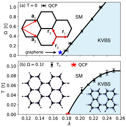
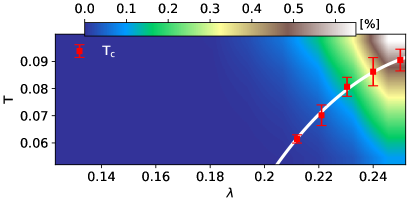
Phase Diagram — Figure 1 shows the zero- and finite- phase diagrams of the half-filled oSSH model on a honeycomb lattice, which are our main results. In both cases, we see the emergence of a KVBS state from a SM phase, with no indication of additional antiferromagentic (AFM), charge-density-wave, or superconducting orders [43].
Figure 1(a) plots the model’s ground-state - phase diagram. The KVBS phase is characterized by both electronic bond correlations and a static periodic distortion of the lattice, pictured in the right inset. These Kekulé lattice distortions are strongest in the adiabatic limit and correspond to the “Kek-O” phase characterized by a supercell in which a central hexagon isotropically expands while the six adjacent hexagons contract via an alternating pattern of expanded and contracted bonds. Increasing enhances quantum fluctuations of the lattice, which disrupt the pattern of Kekulé lattice distortions and shift the SM-KVBS phase boundary to larger .
The star in Fig. 1(a) indicates the approximate parameters corresponding to graphene. The relevant phonon modes in graphene are the and modes with energy [31, 45, 46]. The lattice distortions associated with the phonon mode are consistent with the KVBS state, and couple to the electrons by modulating the nearest-neighbor hopping amplitude. We estimate the strength of this coupling as with a corresponding [43]. As expected, monolayer graphene falls in the SM region of the phase diagram but lies very close to the SM-KVBS phase boundary. Thus, small perturbations that increase , as may be expected to accompany the application of an isotropic strain, could drive the emergence of a KVBS state [18].
Figure 1(b) shows the model’s - phase diagram for fixed phonon energy , where a phase transition to the KVBS state appears above a critical coupling . Previous investigations of this phase transition in purely electronic models indicate that it is weakly first-order at finite temperature but becomes second-order at the QCP, with the quantum phase transition being in the Chiral XY universality class. Our results are consistent with a weakly first-order finite temperature transition in the oSSH model. However, they suggest that the transition remains weakly first-order down to instead of becoming second-order at the QCP.
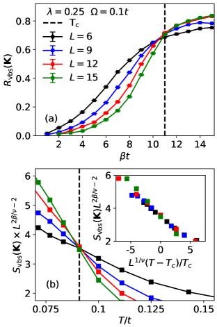
We first consider the finite temperature transition. Since this transition is expected to be weakly first-order [25, 47], we used several approaches to probe its character and determine the critical temperature . Figure 2 presents a finite-size scaling (FSS) analysis of both the the structure factor and correlation ratio for and . Formally, these kinds of FSS analyses are only valid for continuous phase transitions; however, for weakly first-order phase transitions one can obtain a pseudo-scaling behavior for exponents different from the expected universality class but with the correct [48]. The crossing point of in Fig. 2(a) aligns with the one for shown in Fig. 2(b). The inset in Fig. 2(b) shows the corresponding collapse, where the critical exponents and , with an estimated transition temperature of . Given the broken symmetry of the KVBS state, these values differ from the three-state Potts model exponents ( and ) we would expect if the transition were continuous. The transition temperature for other values of reported in Fig. 1(b) were determined using the crossing point for the correlation ratio given , , and .
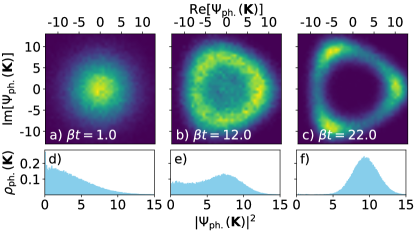
To further probe the symmetry breaking and provide additional evidence suggesting a weakly first-order finite temperature transition, Fig. 3 displays histograms of sampled values of the lattice order parameter for and for an lattice. At [Fig. 3(a)], well above the transition temperature and absent any symmetry breaking, the sampled are symmetrically centered around zero. At [Fig. 2(b)], a temperature near the transition, a ring forms around the origin that is not perfectly radially symmetric. There is also significant weight persisting inside the ring, indicative of the fluctuating first-order nature of the KVBS correlations near . At [Fig. 2(c)], well below the transition temperature, there is no residual weight near zero and three distinct hot spots have formed on the ring, a result of a broken symmetry. Additionally, the location of these three hot spots is consistent with lattice distortions associated with the KVBS state. This behavior is also quite evident in the radial density profiles shown in Figs. 2(d)-(f), which are derived from the histograms shown in panels (a)-(c), respectively.
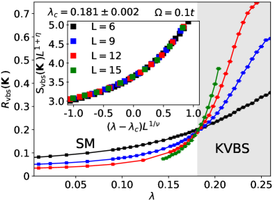
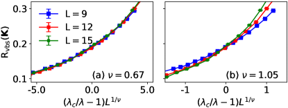
To determine the location of the QCP we again perform a FSS using the correlation ratio , as shown in Fig. 4. Holding the phonon frequency fixed, is given by the crossing point of vs curves for different lattice sizes . This FSS analysis is based on the emergent Lorentz symmetry in the vicinity of the QCP in which depends on and , where . Therefore, we fix in this analysis [49, 50]. Based on the crossing point, we determine that the critical coupling is . The inset then shows the collapse of if we appropriately rescale the axis, treating the critical exponents and as free parameters. We find the optimal collapse with and , values inconsistent with the Chiral XY universality class [24, 25, 27]. Performing a similar collapse of gives a consistent estimate for as well [43]. These observations suggest that the QCP may remain weakly first-order instead of becoming second-order, as observed in similar studies of purely electronic models. The QCP for other values of reported in Fig. 1(a) were determined using lattice sizes , , and .
Discussion — We have presented the ground-state and finite-temperature phase diagrams for the half-filled oSSH model on a honeycomb lattice, investigating the SM-KVBS phase transition. For fixed phonon energy we identify a critical coupling above which the ground-state transitions from a SM to KVBS state. A finite-temperature phase transition to the KVBS state emerges above , with increasing monotonically with . We then estimated the location of graphene in the ground-state phase diagram by assuming the nearest-neighbor electron hopping amplitude couples to the high-energy in-plane bond-stretching phonon mode. The corresponding phonon energy and coupling parameters place graphene in the SM region of the phase diagram, but close to the phase boundary. This result provides new insight into why small perturbations to graphene-derived systems that effectively increase , as is expected to accompany the application of isotropic strain, can drive the system into a KVBS state. This has interesting implications for how strain engineering can be used to tune the electronic properties of graphene-based systems.
Our results also suggest that both the ground-state and finite-temperature SM-KVBS phase transitions are weakly first-order, in agreement with Landau mean-field theory predictions. This result is in contrast with similar QMC investigations of the quantum phase transition in purely electronic models, where coupling to gapless Dirac fermion modes render the QCP second-order, in the Chiral XY universality class. We suspect that our results differ from previous studies as a result retardation effects associated with the -ph interaction, which suppresses quantum fluctuations and have been shown to result in QCPs becoming first-order in other situations as well [51, 52, 53]. For instance, a recent investigation similarly found that lattice fluctuations associated with introducing spin-phonon interactions to the honeycomb Heisenberg model drive the deconfined QCP separating the AFM and KVBS ground-states to be first-order [44].
This work focused on half-filling and absent electronic correlations. It would be interesting to introduce a local repulsive Hubbard interaction to study competition between SM, KVBS, and AFM correlations, as the role of -ph interactions in this scenario has only been treated at the mean-field level [30]. Another avenue would be to study potential pairing with doping, as prior investigations have found that doping a KVBS state led to superconductivity and pseudogap formation [26].
Acknowledgements — This work was supported by the U.S. Department of Energy, Office of Science, Office of Basic Energy Sciences, under Award Number DE-SC0022311. This research used resources of the Oak Ridge Leadership Computing Facility, a DOE Office of Science User Facility supported under Contract No. DE-AC05-00OR22725.
Appendix A DQMC simulations
To obtain our results we ran simulations with 12 walkers in parallel, each performing HMC thermalization updates with HMC measurement updates. Throughout, we set the imaginary-time discretization to . Each HMC update was performed using time-steps, with the step-size given by . We used refer to Ref. [41] for more information regarding the details of the HMC algorithm.
Appendix B Parameter estimates for graphene
The relevant phonon modes at the Dirac points in graphene are associated with and phonon branches, with corresponding energies of [31, 45, 46]. The lattice distortions associated with the and phonons are consistent with the Kekulé lattice distortion pattern observed in our DQMC simulations. To estimate the coupling strength , we consider the functional form for the hopping amplitude
| (3) |
which is commonly used in the literature for small changes in the equilibrium bond length . Here, is the lattice parameter in the semi-metal phase, , and [54]. Thus, the -ph coupling strength in the linear approximation is . The corresponding dimensionless coupling in our notation is
| (4) |
where is the mass of carbon and .

Appendix C Hopping inversion and Phase
In Su-Schrieffer-Heeger (SSH) models, phonon displacements modulate the nearest neighbor hopping amplitude. At linear order in the atomic displacements, the effective hopping is parameterized as in Eq. (3) and can change sign for sufficiently large coupling strength and lattice displacements . When this occurs, the sign of the effective hopping integral inverts, which induces significant changes in the model’s ground and excited state properties [55, 36]. It is important to note that such sign changes are not physical but rather a byproduct of the linear approximation for the -ph interaction (see Sec. B).
Our implementation of the DQMC algorithm does not place any restrictions on the phonon displacements, so it is possible for to be negative. To ensure this does not happen in our model, we measure what percentage of the time this occurs as
| (5) |
where is the Heaviside function. Fig. 5 plots the evolution of this quantity as a function of temperature and dimensionless coupling for our simulations performed on an site cluster. The results indicate that a hopping inversion rarely occurs (less than 0.5%) over the entire range of parameters and that such inversions occur more frequently at high temperatures, where large thermal fluctuations form, or at strong -ph coupling. Interestingly, the heat map shows that there is no direct relation between hopping inversion frequency and the formation of the KVBS phase.
Appendix D Additional information on the SM-KVBS phase transition
The KVBS structure factor may be expressed as
| (6) | ||||
where
| (7) |
is the equal-time bond-structure factor between bonds and , measured at the scattering momentum connecting the two Dirac points. Fig. 6 plots a heat map for an lattice with . The red line indicates the best fit line we obtain for transition temperature of the SM-KVBS transition. The heat-map matches well with the estimated values, with larger values appearing in the KVBS phase.
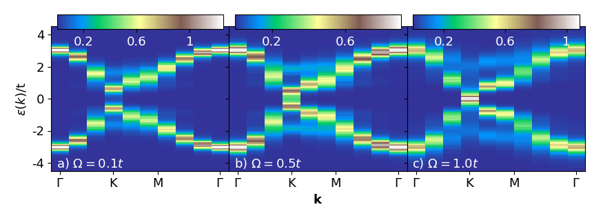
Appendix E Results for the electron spectral function
Figure 7 provides supplementary results for the single-particle spectral function as a function of phonon energy and a fixed -ph coupling . For (Fig. 7a), the system is in the KVBS phase and a gap forms in at the Dirac point. As the phonon energy is increased, the size of the gap decreases for (Fig. 7b) and ultimately closes for (Fig. 7c). These results are in line with the theoretical prediction that this particular KVBS order (“Kek-O” order) induces a gap at the Dirac point.
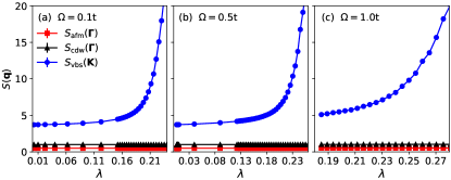
Appendix F Absence of competing charge-density-wave or antiferromagnetic correlations
Figure 8 shows results for the charge-density-wave (CDW), AFM, and KVBS structure factors at fixed . The measurements show an absence of CDW and AFM phases for the given range. The CDW and AFM structure factors are given by
| (8) |
and
| (9) |
respectively, where and are the total electron number and spin- operators for orbital in unit cell . The definition of is provided in the main text.
Appendix G Finite Size Scaling Collapse
Figure 9 shows the collapses of using two different values for the critical exponent . The left panel is for , the optimal value obtained based on the collapse reported in the main text. The panel on the right shows the collapse for , a value previously reported for the chiral XY universality class [24, 30]. The results in a better collapse of the data compared to the results.
References
- Novoselov et al. [2004] K. S. Novoselov, A. K. Geim, S. V. Morozov, D.-e. Jiang, Y. Zhang, S. V. Dubonos, I. V. Grigorieva, and A. A. Firsov, Electric field effect in atomically thin carbon films, science 306, 666 (2004).
- Novoselov et al. [2005] K. S. Novoselov, A. K. Geim, S. V. Morozov, D. Jiang, M. I. Katsnelson, I. V. Grigorieva, S. V. Dubonos, and A. A. Firsov, Two-dimensional gas of massless dirac fermions in graphene, Nature 438, 197 (2005).
- Castro Neto et al. [2009] A. H. Castro Neto, F. Guinea, N. M. R. Peres, K. S. Novoselov, and A. K. Geim, The electronic properties of graphene, Rev. Mod. Phys. 81, 109 (2009).
- Du et al. [2008] X. Du, I. Skachko, A. Barker, and E. Y. Andrei, Approaching ballistic transport in suspended graphene, Nature Nanotechnology 3, 491 (2008).
- Zhang et al. [2005] Y. Zhang, Y.-W. Tan, H. L. Stormer, and P. Kim, Experimental observation of the quantum Hall effect and Berry’s phase in graphene, Nature 438, 201 (2005).
- Beenakker [2008] C. W. J. Beenakker, Colloquium: Andreev reflection and Klein tunneling in graphene, Rev. Mod. Phys. 80, 1337 (2008).
- Naumis et al. [2023] G. G. Naumis, S. A. Herrera, S. P. Poudel, H. Nakamura, and S. Barraza-Lopez, Mechanical, electronic, optical, piezoelectric and ferroic properties of strained graphene and other strained monolayers and multilayers: an update, Rep. Prog. Phys 87, 016502 (2023).
- Cao et al. [2018a] Y. Cao, V. Fatemi, A. Demir, S. Fang, S. L. Tomarken, J. Y. Luo, J. D. Sanchez-Yamagishi, K. Watanabe, T. Taniguchi, E. Kaxiras, et al., Correlated insulator behaviour at half-filling in magic-angle graphene superlattices, Nature 556, 80 (2018a).
- Cao et al. [2018b] Y. Cao, V. Fatemi, S. Fang, K. Watanabe, T. Taniguchi, E. Kaxiras, and P. Jarillo-Herrero, Unconventional superconductivity in magic-angle graphene superlattices, Nature 556, 43 (2018b).
- Bao et al. [2021] C. Bao, H. Zhang, T. Zhang, X. Wu, L. Luo, S. Zhou, Q. Li, Y. Hou, W. Yao, L. Liu, P. Yu, J. Li, W. Duan, H. Yao, Y. Wang, and S. Zhou, Experimental evidence of chiral symmetry breaking in Kekulé-ordered graphene, Phys. Rev. Lett. 126, 206804 (2021).
- Gutiérrez et al. [2016] C. Gutiérrez, C.-J. Kim, L. Brown, T. Schiros, D. Nordlund, E. B. Lochocki, K. M. Shen, J. Park, and A. N. Pasupathy, Imaging chiral symmetry breaking from Kekulé bond order in graphene, Nature Physics 12, 950 (2016).
- Hou et al. [2007] C.-Y. Hou, C. Chamon, and C. Mudry, Electron fractionalization in two-dimensional graphenelike structures, Phys. Rev. Lett. 98, 186809 (2007).
- Lin et al. [2017] Z. Lin, W. Qin, J. Zeng, W. Chen, P. Cui, J.-H. Cho, Z. Qiao, and Z. Zhang, Competing gap opening mechanisms of monolayer graphene and graphene nanoribbons on strong topological insulators, Nano letters 17, 4013 (2017).
- Wu and Hu [2016] L.-H. Wu and X. Hu, Topological properties of electrons in honeycomb lattice with detuned hopping energy, Scientific Reports 6, 24347 (2016).
- Blason and Fabrizio [2022] A. Blason and M. Fabrizio, Local Kekulé distortion turns twisted bilayer graphene into topological Mott insulators and superconductors, Phys. Rev. B 106, 235112 (2022).
- Liu et al. [2017] Y. Liu, C.-S. Lian, Y. Li, Y. Xu, and W. Duan, Pseudospins and topological effects of phonons in a Kekulé lattice, Phys. Rev. Lett. 119, 255901 (2017).
- Frank and Lieb [2011] R. L. Frank and E. H. Lieb, Possible lattice distortions in the hubbard model for graphene, Phys. Rev. Lett. 107, 066801 (2011).
- Sorella et al. [2018] S. Sorella, K. Seki, O. O. Brovko, T. Shirakawa, S. Miyakoshi, S. Yunoki, and E. Tosatti, Correlation-driven dimerization and topological gap opening in isotropically strained graphene, Phys. Rev. Lett. 121, 066402 (2018).
- Eom and Koo [2020] D. Eom and J.-Y. Koo, Direct measurement of strain-driven Kekulé distortion in graphene and its electronic properties, Nanoscale 12, 19604 (2020).
- Sugawara et al. [2011] K. Sugawara, K. Kanetani, T. Sato, and T. Takahashi, Fabrication of Li-intercalated bilayer graphene, Aip Advances 1 (2011).
- Kanetani et al. [2012] K. Kanetani, K. Sugawara, T. Sato, R. Shimizu, K. Iwaya, T. Hitosugi, and T. Takahashi, Ca intercalated bilayer graphene as a thinnest limit of superconducting C6Ca, Proceedings of the National Academy of Sciences 109, 19610 (2012).
- Qu et al. [2022] A. C. Qu, P. Nigge, S. Link, G. Levy, M. Michiardi, P. L. Spandar, T. Matthé, M. Schneider, S. Zhdanovich, U. Starke, et al., Ubiquitous defect-induced density wave instability in monolayer graphene, Science advances 8, eabm5180 (2022).
- Cheianov et al. [2009] V. Cheianov, V. Fal’ko, O. Syljuåsen, and B. Altshuler, Hidden Kekulé ordering of adatoms on graphene, Solid State Communications 149, 1499 (2009).
- Li et al. [2017] Z.-X. Li, Y.-F. Jiang, S.-K. Jian, and H. Yao, Fermion-induced quantum critical points, Nature communications 8, 314 (2017).
- Xu et al. [2018] X. Y. Xu, K. T. Law, and P. A. Lee, Kekulé valence bond order in an extended Hubbard model on the honeycomb lattice with possible applications to twisted bilayer graphene, Phys. Rev. B 98, 121406 (2018).
- Li et al. [2023] Z.-X. Li, S. G. Louie, and D.-H. Lee, Emergent superconductivity and non-fermi liquid transport in a doped valence bond solid insulator, Phys. Rev. B 107, L041103 (2023).
- Da Liao et al. [2019] Y. Da Liao, Z. Y. Meng, and X. Y. Xu, Valence bond orders at charge neutrality in a possible two-orbital extended Hubbard model for twisted bilayer graphene, Phys. Rev. Lett. 123, 157601 (2019).
- Zhang et al. [2021] H. Zhang, C. Bao, M. Schüler, S. Zhou, Q. Li, L. Luo, W. Yao, Z. Wang, T. P. Devereaux, and S. Zhou, Self-energy dynamics and the mode-specific phonon threshold effect in Kekulé-ordered graphene, National Science Review 9, nwab175 (2021).
- Classen et al. [2014] L. Classen, M. M. Scherer, and C. Honerkamp, Instabilities on graphene’s honeycomb lattice with electron-phonon interactions, Phys. Rev. B 90, 035122 (2014).
- Otsuka and Yunoki [2024] Y. Otsuka and S. Yunoki, Kekulé valence bond order in the Hubbard model on the honeycomb lattice with possible lattice distortions for graphene, Phys. Rev. B 109, 115131 (2024).
- Wu et al. [2018] F. Wu, A. H. MacDonald, and I. Martin, Theory of phonon-mediated superconductivity in twisted bilayer graphene, Phys. Rev. Lett. 121, 257001 (2018).
- Lian et al. [2019] B. Lian, Z. Wang, and B. A. Bernevig, Twisted bilayer graphene: A phonon-driven superconductor, Phys. Rev. Lett. 122, 257002 (2019).
- Zhang et al. [2019] Y.-X. Zhang, W.-T. Chiu, N. C. Costa, G. G. Batrouni, and R. T. Scalettar, Charge order in the Holstein model on a honeycomb lattice, Phys. Rev. Lett. 122, 077602 (2019).
- Chen et al. [2019] C. Chen, X. Y. Xu, Z. Y. Meng, and M. Hohenadler, Charge-density-wave transitions of Dirac fermions coupled to phonons, Phys. Rev. Lett. 122, 077601 (2019).
- Bradley et al. [2023] O. Bradley, B. Cohen-Stead, S. Johnston, K. Barros, and R. T. Scalettar, Charge order in the kagome lattice Holstein model: a hybrid Monte Carlo study, npj Quantum Materials 8, 21 (2023).
- Malkaruge Costa et al. [2023] S. Malkaruge Costa, B. Cohen-Stead, A. Tanjaroon Ly, J. Neuhaus, and S. Johnston, Comparative determinant quantum monte carlo study of the acoustic and optical variants of the Su-Schrieffer-Heeger model, Phys. Rev. B 108, 165138 (2023).
- Tanjaroon Ly et al. [2023] A. Tanjaroon Ly, B. Cohen-Stead, S. Malkaruge Costa, and S. Johnston, Comparative study of the superconductivity in the holstein and optical Su-Schrieffer-Heeger models, Phys. Rev. B 108, 184501 (2023).
- Beyl et al. [2018] S. Beyl, F. Goth, and F. F. Assaad, Revisiting the hybrid quantum Monte Carlo method for Hubbard and electron-phonon models, Phys. Rev. B 97, 085144 (2018).
- Batrouni and Scalettar [2019] G. G. Batrouni and R. T. Scalettar, Langevin simulations of a long-range electron-phonon model, Phys. Rev. B 99, 035114 (2019).
- Cohen-Stead et al. [2022] B. Cohen-Stead, O. Bradley, C. Miles, G. Batrouni, R. Scalettar, and K. Barros, Fast and scalable quantum Monte Carlo simulations of electron-phonon models, Phys. Rev. E 105, 065302 (2022).
- Cohen-Stead et al. [2024a] B. Cohen-Stead, S. M. Costa, J. Neuhaus, A. T. Ly, Y. Zhang, R. Scalettar, K. Barros, and S. Johnston, SmoQyDQMC.jl: A flexible implementation of determinant quantum Monte Carlo for Hubbard and electron-phonon interactions (2024a).
- Cohen-Stead et al. [2024b] B. Cohen-Stead, S. M. Costa, J. Neuhaus, A. T. Ly, Y. Zhang, R. Scalettar, K. Barros, and S. Johnston, Codebase release r0.3 for SmoQyDQMC.jl, SciPost Phys. Codebases , 29 (2024b).
- [43] See online supplementary materials for additional details on our DQMC simulations, avaialble at link to be supplied by the publisher.
- Weber [2021] M. Weber, Valence bond order in a honeycomb antiferromagnet coupled to quantum phonons, Phys. Rev. B 103, L041105 (2021).
- Basko [2007] D. M. Basko, Effect of inelastic collisions on multiphonon Raman scattering in graphene, Phys. Rev. B 76, 081405 (2007).
- Basko and Aleiner [2008] D. M. Basko and I. L. Aleiner, Interplay of Coulomb and electron-phonon interactions in graphene, Phys. Rev. B 77, 041409 (2008).
- Zhou et al. [2016] Z. Zhou, D. Wang, Z. Y. Meng, Y. Wang, and C. Wu, Mott insulating states and quantum phase transitions of correlated Dirac fermions, Phys. Rev. B 93, 245157 (2016).
- Iino et al. [2019] S. Iino, S. Morita, N. Kawashima, and A. W. Sandvik, Detecting signals of weakly first-order phase transitions in two-dimensional Potts models, Journal of the Physical Society of Japan 88, 034006 (2019).
- Assaad and Herbut [2013] F. F. Assaad and I. F. Herbut, Pinning the order: The nature of quantum criticality in the Hubbard model on honeycomb lattice, Phys. Rev. X 3, 031010 (2013).
- Herbut et al. [2009] I. F. Herbut, V. Juričić, and B. Roy, Theory of interacting electrons on the honeycomb lattice, Phys. Rev. B 79, 085116 (2009).
- Sarkar et al. [2023] S. Sarkar, L. Franke, N. Grivas, and M. Garst, Quantum criticality on a compressible lattice, Phys. Rev. B 108, 235126 (2023).
- Samanta et al. [2022] A. Samanta, E. Shimshoni, and D. Podolsky, Phonon-induced modification of quantum criticality, Phys. Rev. B 106, 035154 (2022).
- Chandra et al. [2020] P. Chandra, P. Coleman, M. A. Continentino, and G. G. Lonzarich, Quantum annealed criticality: A scaling description, Phys. Rev. Res. 2, 043440 (2020).
- Ribeiro et al. [2009] R. Ribeiro, V. M. Pereira, N. Peres, P. Briddon, and A. C. Neto, Strained graphene: tight-binding and density functional calculations, New Journal of Physics 11, 115002 (2009).
- Banerjee et al. [2023] D. Banerjee, J. Thomas, A. Nocera, and S. Johnston, Ground-state and spectral properties of the doped one-dimensional optical Hubbard-Su-Schrieffer-Heeger model, Phys. Rev. B 107, 235113 (2023).