Universal and non-universal signatures in the scaling functions of critical variables
Abstract
The view that the probability density function (PDF) of a key statistical variable, anomalously scaled by size or time, could furnish a hallmark of universal behavior contrasts with the circumstance that such density sensibly depends on non-universal features. We solve this apparent contradiction by demonstrating that both non-universal amplitudes and universal exponents of leading critical singularities in large deviation functions are determined by the PDF tails, whose form is argued on extensivity. This unexplored scenario implies a universal form of central limit theorem at criticality and is confirmed by exact calculations for mean field Ising models in equilibrium and for anomalous diffusion models.
The confirmation of scaling and universality, together with the calculation of critical exponents on which one can test such universality, are among the most fundamental achievements of the theory of equilibrium critical phenomena [1, 2, 3]. Much progress in this field was possible through finite size scaling techniques, which allowed to determine critical exponents by extrapolating to the thermodynamic limit finite systems properties [4, 5, 6]. An interesting prerogative of finite systems at criticality is also the fact that the probability distribution of the order parameter, if properly scaled, converges to a well defined scaling PDF [7, 8]. For example, in an Ising model with spins in dimensions, the probability distribution of the magnetization at the critical temperature and in zero magnetic field is expected to converge for increasing to a limit
| (1) |
with a scaling function of the rescaled magnetization , and the magnetic Kadanoff exponent [3].
Scaling functions were proposed as possible locations of universal signatures, with a conjectured stretched exponential decay for large [9, 10] modulated by the equation of state exponent [3] and some unknown coefficient . In spite of many attempts, numerical analyses of proved to be extremely difficult and far from conclusive for the tails [11, 12, 13, 14] (for rigorous proofs in 2D see [15, 16]). Analytical evidence of this type of decay, with precisely the form conjectured for the Ising magnetization scaling function [9, 10] 111This form also included a power law factor multiplying the stretched exponential. However, this factor does not influence extensive quantities., was most recently found in a series of paradigmatic models of anomalous diffusion [18, 19] with time and displacement playing the roles of system’s size and magnetization, respectively. Such decay was also identified as responsible of power law singularities in the large deviation functions of displacement, suggesting the importance of these models for proving properties out of reach in the Ising case.
The probabilistic interpretation of the renormalization group [20, 21] suggested to regard non-Gaussian scaling functions as solutions of stability conditions for the PDF’s of sums of strongly correlated random variables [22, 23]. It remains an open issue to identify up to what extent these shapes are reflecting universal (or non-universal 222Typical non-universal quantities are the amplitudes of the power law singularities, which can be of key importance also in the numerical or experimental identification of the exponents themselves.) properties, as strongly depends on features which can be different within the same universality class, such as the boundary conditions of the finite systems from which it is extrapolated [7, 25, 26]. The absence of precise criteria for identifying universal and non-universal features of scaling functions prevented so far the formulation of general forms of limit theorems at equilibrium criticality, as well as a thorough investigation of critical power-law singularities in the rate functions of large deviation theory [27, 28, 29].
In this work, we focus on the magnetization of the critical Ising model in equilibrium as a paradigmatic example of variable obeying anomalous scaling. We demonstrate that the extensivity of an auxiliary form of cumulant generator determines the stretched exponential decay of the scaling function conjectured for the Ising model. This decay is shown to account for both universal exponents and non-universal amplitudes of leading singularities in all large deviation functions, opening to a universal generalization of the central limit theorem at criticality. The scenario is exactly confirmed in the case of mean field interactions and for the displacement in time of anomalous diffusion models.
We start by considering the example of an Ising model in equilibrium. In or , the system undergoes a phase transition at a finite critical temperature [3]. We consider a box with spins, e.g. on a square or cubic lattice, and with open boundary conditions. The same argument applies to different lattices or periodic boundary conditions. Given a generic configuration of the system, where is the spin at site , the total magnetization is . The system has reduced Hamiltonian . Here is a ferromagnetic coupling and the sum is extended to all pairs of nearest neighbor sites, is the Boltzmann’s constant and is a dimensionless magnetic field (magnetic spin energy divided by ; the same analysis can be repeated for negative ). The reduced Helmoltz free energy is given by where the sum is over all spin configurations and the following identity holds (see the Supplemental Material [30]):
| (2) |
Here, is the probability of observing the system in a generic configuration with total magnetization for . Thus, refers to the system becoming critical in the thermodynamic limit. The function is the generator of the cumulants of this probability distribution by derivation with respect to at .
If we set in Eq. 2 for large the right hand side should grow as , where is the free energy per site in the thermodynamic limit (the dots represent sub-extensive terms that depend on the specific choice of boundary conditions 333Surface terms or edge free energies for open boundary conditions lead to contributions proportional to or , while corners yield terms . These corrections are absent for periodic boundary conditions, while an -independent Privman-Fisher coefficient [6], possibly dependent on boundary conditions, should be always present.). In large deviations language is the scaled cumulant generating function (SCGF) [27] of the observable at , with playing the role of a Laplace parameter. We expect to be singular at criticality for [3], so that we can write
| (3) |
where the first term on the r.h.s. is the leading singular term with amplitude and the dots indicate other less singular or regular terms in a whole expansion (sub-extensive terms in Eq. 2 are omitted). The determination of the leading singular term, with the magnetic Kadanoff exponent , is a task which can be faced only by exact solutions (in 2D [15]) and in most cases is more or less satisfactorily achieved by approximate numerical or renormalization group methods [4, 1, 3].
At criticality, is expected to satisfy scaling as , meaning that in the thermodynamic limit this distribution translates into a PDF (up to a factor , see [30]) of the continuous argument . Here we want to show that the elusive behavior of for large can be obtained by studying the role of this function in characterizing the limit in Eq. 3. At the same time, we will demonstrate that this insight is sufficient to fully characterize the correct exponent and amplitude of the leading singularity of . Quite remarkably, given the value of , the form of the asymptotic behavior of can be argued simply on the basis of the extensivity of the cumulant generator (the power of normalizing in Eq. 3). This extensivity in equilibrium is determined by the existence of the thermodynamic limit for the free energy density.
To accomplish all this, one has to replace by an auxiliary expression defined as
| (4) |
which, by differentiation with respect to at , generates the leading large behavior of the moments of . As we show below, cannot be expected to reproduce the full large behavior (inclusive of sub-leading extensive terms) on the r.h.s. of Eq. 3. Indeed, is a function of the single argument , instead of and separately as . Still, offers the advantage to fully account for the leading singularity just by inspection of its behavior. At the same time, this generator allows to link this singularity to the tail of .
Assuming rapid decay of at large , the integral in Eq. 4 for large is dominated by the maximum value of the integrand. For , the point of maximum of the integrand approaches in the limit . Writing , formally satisfies the differential equation
| (5) |
such that the leading contribution to the logarithm of the auxiliary function is
| (6) |
Now, if this leading contribution is assumed to be and , from the last two equations follows that and . This necessarily implies that must be proportional to a power of . Indeed, is expected to grow as , but a growth faster than a power, e.g. exponential, would lead to , not fulfilling the required extensivity. Following the notations adopted in Refs. [9, 32], we write and, consistently,
| (7) |
These positions are clearly compatible with Eq. 5 and, guarantee a leading Laplace contribution to the logarithm of the integral in Eq. 4 with
| (8) |
as it can be verified in Eq. 6. Indeed, upon substitution we get
| (9) |
yielding the expected leading magnetic singularity of the free energy density of the model (Eq. 3).
We propose to interpret the factor multiplying on the r.h.s. of Eq. 9 as the amplitude of the singularity in of the free energy density at (the coefficient in Eq. 3). While such an amplitude is generally expected to be non-universal [6], its estimation through the auxiliary function suggests that it depends only on the universal exponent and the coefficient multiplying in the exponential decay rate of . A direct verification that Eq. 9 provides precisely the amplitude of the leading singularity in of the free energy density in 2 or 3D is not possible. However, our exact results for mean field interactions and for anomalous diffusion models provide strong indirect confirmation (see below).
The role played by the constant in the decay rate of acquires further importance if we look at the consequences of Eq. 9 for the rate function in terms of which one expresses the large deviation principle for the magnetization density . This principle can be formulated by saying that for large one has
| (10) |
The validity of this large deviation principle is guaranteed here by Gärtner-Ellis theorem [33, 34], since the condition guarantees that is differentiable for all . According to this theorem, we can obtain the rate function through a Legendre-Fenchel Transform of the SCGF as
| (11) |
Such a supremum problem implies solving for the equation . This can be easily done in the neighborhood of , where the dependence of just reduces to the leading singular term in Eq. 9. Substituting in the expression of which we need to compute the in Eq. 11, one obtains , valid for . This shows that the amplitude of the power law singularity of is identical to the coefficient appearing in the exponential decay rate of for large . This establishes a precise link between the singularity of the rate function at its minimum , and the tail of the scaling function for large . For critical Ising models, rate functions have been extensively studied, by numerical or renormalization group methods [29]. However, so far, these studies did not establish for them general features related to universal critical exponents or to critical amplitudes.
Ising Mean-Field – An exact confirmation of the established above link between scaling and rate functions at criticality is possible in the case of an Ising model in which the spin-spin interaction is expressed in a mean field way as . This allows to write explicitly the magnetization probability in zero external field as (see SM [30])
| (12) |
The critical temperature is easily determined to be by cancellation of the quadratic term, implying a quartic rate function at criticality . This mean field rate function allows for an exact verification of the connection between its amplitude around at criticality with the scaling function tail.
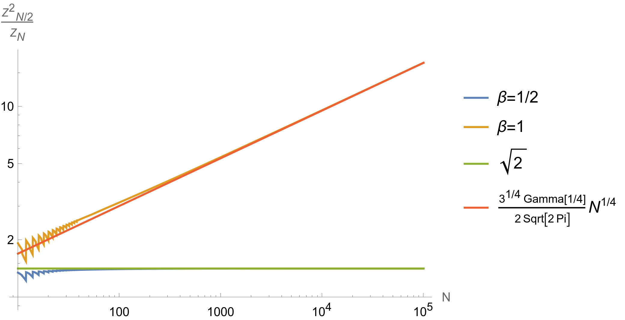
Since for the mean field case we should have , we argue that a plausible scaled variable is , which indeed cancels the asymptotic dependence on in the fourth order term. So, for this model in which looses meaning, is replaced by in our basic Eq. 4. The problem left is to determine . Such a task was faced long ago by Ellis and Newman [35, 36] (see also [22]), with a derivation within a renormalization group strategy that proposed to identify the scaling function among a parameterized infinity of possible fixed point solutions which, however, does not include normalized PDFs. In the Supplemental Material [30], we present a consistent derivation of the scaling function for all by showing that at criticality it exactly satisfies the stability condition
| (13) |
under iterative doubling of the number of spins in the limit of infinite system, where is the complete Gamma function. The unique solution of this fixed point equation is
| (14) |
which is the (normalized) scaling function for the mean-field Ising model. The exponential decay rate for exactly coincides, both in exponent and in amplitude, with the leading term of around , as predicted by our general argument.
Central limit theorems – Another aim of the present investigation is to explore general, possibly universal, forms of limit theorems valid at criticality. While the full knowledge of a scaling function would amount automatically to a limit theorem [37], the existence of dependencies on boundary conditions of the critical scaling functions [26, 25] represents a manifest obstacle to the achievement of such generality. Our result concerning the asymptotic decay of scaling functions for large argument suggests validity of a weak form of generalized central limit theorem [27] for additive observables like the magnetization of the Ising model at criticality. Indeed, the behavior we found for around , suggests that one can approximate the PDF of values not too deviating from as
| (15) |
depending only on and on the universal exponent . As in the case of the standard central limit theorem, recovered here for , one should expect that this approximation works well for magnetization values if sub-leading contributions to are of order sufficiently higher than .
Of key importance for the above derivations has been the possibility to extract the leading singular term of the free energy by performing the limit for (thus, at arbitrary nonzero ) of the integral in Eq. 4. This term is obtained without having previously performed an limit to extract the full in Eq. 3.
Anomalous Diffusion – Outside of equilibrium, large deviation theory can be used to describe the behavior of key extensive variables, such as the total particle transfer [38, 39, 40, 27, 41, 42, 43, 44, 45, 46, 47] or entropy production [48, 49, 50]. Dynamical large deviation functions in these contexts have been shown to exhibit singular behaviors, but typically related to first order transitions [51, 52, 53, 54, 55, 56, 57, 58]. Here we show that the derivation we outlined for the magnetization of the Ising model in equilibrium holds also for extensive variables exhibiting anomalous scaling out of equilibrium, ultimately leading to critical power-law singularities in the rate function. Indeed, strong support to the validity of the above Ising scenario comes from the context of anomalous diffusion, in which the mean squared displacement of a diffusing particle grows as with and diffusion constant [59, 18, 19]. In these dynamical contexts, displacement plays the role of magnetization, while the system’s extensivity is regulated by time in place of size. Exact results can be obtained in the 1D Continuous Time Random Walk model (CTRW), in which a particle hops with some rate (in units ) to nearest neighboring sites on a lattice with spacing . The probability of observing a particle at a position of a 1D lattice evolves according to
| (16) |
where the fractional Caputo [60] derivative accounts for the power-law tailed waiting time PDF giving rise to subdiffusion [61]. The generating function of displacement and the associated SCGF can be evaluated exactly for this model (see [30, 18, 50]) providing the singular behavior
| (17) |
Here the Laplace parameter acts as the magnetic field in the Ising case, so that can be regarded as an analog of .
Taking the continuum limit, the lattice spacing goes to zero while stays constant and the probability distribution approaches the PDF of the continuous displacement . From Eq. 16 we get that this PDF satisfies the fractional diffusion equation , whose solution can be expressed as with M-Wright function [62, 63, 64, 61]. This allows to conclude that the scaling function is with rescaled displacement , so that we can write
| (18) |
For large the M-Wright function is known exactly [62] to have a stretched exponential decay
| (19) |
This is consistent with , equivalent to Eq. 8, and expressing the Fisher relation for anomalous diffusion [65, 18, 19]. Plugging and the coefficient implied by the last equation into the equivalent of Eq. 9, and taking into account that , eventually yields the same leading singularity in obtained in Eq. 17. On the basis of this singularity one can also argue the behavior of the rate function around , obtaining [30]
| (20) |
Summarizing, we have shown that plausible arguments allow to argue the exponential decay rate of the scaling function of a critical observable and to fully characterize the leading singularity of the SCGF in terms of this rate. We did also establish the existence of a critical singularity of the rate function of large deviation theory at its minimum, with exponent and amplitude matching precisely those of this exponential decay rate. This singularity guarantees validity of a general form of central limit theorem for additive critical variables. The whole scenario must be expected to hold for both equilibrium and non-equilibrium variables obeying anomalous scaling with scaling function possessing finite moments of all orders. Altogether the results show the central role played by scaling function tails in setting up a large deviations approach to criticality. They also strongly support and extend, as far as meaning and implications are concerned, long standing unproved conjectures for equilibrium Ising criticality.
Acknowledgements.
G. T. is supported by the Center for Statistical Mechanics at the Weizmann Institute of Science, the grant 662962 of the Simons foundation, the grants HALT and Hydrotronics of the EU Horizon 2020 program and the NSF-BSF grant 2020765. We thank Marzio Cassandro for advice and useful remarks in early stages of this project, as well as Giovanni Jona-Lasinio, Giovanni Gallavotti, Mehran Kardar, Hugo Touchette, David Mukamel, Oren Raz, and Amos Maritan for useful discussions and remarks.References
- Goldenfeld [2018] N. Goldenfeld, Lectures on phase transitions and the renormalization group (CRC Press, 2018).
- Cardy [1996] J. Cardy, Scaling and renormalization in statistical physics, Vol. 5 (Cambridge university press, 1996).
- Kadanoff [2000] L. P. Kadanoff, Statistical physics: statics, dynamics and renormalization (World Scientific, 2000).
- Privman [1990] V. Privman, Finite size scaling and numerical simulation of statistical systems (World Scientific, 1990).
- Cardy [2012] J. Cardy, Finite-size scaling (Elsevier, 2012).
- Privman and Fisher [1984] V. Privman and M. E. Fisher, Universal critical amplitudes in finite-size scaling, Phys. Rev. B 30, 322 (1984).
- Binder [1981] K. Binder, Finite size scaling analysis of ising model block distribution functions, Zeitschrift für Physik B Condensed Matter 43, 119 (1981).
- Nicolaides and Bruce [1988] D. Nicolaides and A. Bruce, Universal configurational structure in two-dimensional scalar models, Journal of Physics A: Mathematical and General 21, 233 (1988).
- Bruce [1995] A. Bruce, Critical finite-size scaling of the free energy, Journal of Physics A: Mathematical and General 28, 3345 (1995).
- Hilfer and Wilding [1995] R. Hilfer and N. Wilding, Are critical finite-size scaling functions calculable from knowledge of an appropriate critical exponent?, Journal of Physics A: Mathematical and General 28, L281 (1995).
- Tsypin and Blöte [2000] M. M. Tsypin and H. W. J. Blöte, Probability distribution of the order parameter for the three-dimensional ising-model universality class: A high-precision monte carlo study, Phys. Rev. E 62, 73 (2000).
- Hilfer et al. [2003] R. Hilfer, B. Biswal, H. G. Mattutis, and W. Janke, Multicanonical monte carlo study and analysis of tails for the order-parameter distribution of the two-dimensional ising model, Phys. Rev. E 68, 046123 (2003).
- Hilfer et al. [2005] R. Hilfer, B. Biswal, H.-G. Mattutis, and W. Janke, Multicanonical simulations of the tails of the order-parameter distribution of the two-dimensional ising model, Computer physics communications 169, 230 (2005).
- Malakis and Fytas [2006] A. Malakis and N. G. Fytas, Universal features and tail analysis of the order-parameter distribution of the two-dimensional ising model: An entropic sampling monte carlo study, Phys. Rev. E 73, 056114 (2006).
- McCoy and Wu [1973] B. M. McCoy and T. T. Wu, The two-dimensional Ising model (Harvard University Press, 1973).
- Camia et al. [2016] F. Camia, C. Garban, and C. M. Newman, Planar Ising magnetization field II. Properties of the critical and near-critical scaling limits, Annales de l’Institut Henri Poincaré, Probabilités et Statistiques 52, 146 (2016).
- Note [1] This form also included a power law factor multiplying the stretched exponential. However, this factor does not influence extensive quantities.
- Stella et al. [2023a] A. L. Stella, A. Chechkin, and G. Teza, Anomalous dynamical scaling determines universal critical singularities, Phys. Rev. Lett. 130, 207104 (2023a).
- Stella et al. [2023b] A. L. Stella, A. Chechkin, and G. Teza, Universal singularities of anomalous diffusion in the richardson class, Phys. Rev. E 107, 054118 (2023b).
- Jona-Lasinio [1975] G. Jona-Lasinio, The renormalization group: A probabilistic view, Il Nuovo Cimento B (1971-1996) 26, 99 (1975).
- Jona-Lasinio [2001] G. Jona-Lasinio, Renormalization group and probability theory, Physics Reports 352, 439 (2001).
- Cassandro and Jona-Lasinio [1978] M. Cassandro and G. Jona-Lasinio, Critical point behaviour and probability theory, Advances in Physics 27, 913 (1978).
- Gallavotti and Martin-Löf [1975] G. Gallavotti and A. Martin-Löf, Block-spin distributions for short-range attractive ising models, Il Nuovo Cimento B (1971-1996) 25, 425 (1975).
- Note [2] Typical non-universal quantities are the amplitudes of the power law singularities, which can be of key importance also in the numerical or experimental identification of the exponents themselves.
- Antal et al. [2004] T. Antal, M. Droz, and Z. Rácz, Probability distribution of magnetization in the one-dimensional ising model: effects of boundary conditions, Journal of Physics A: Mathematical and General 37, 1465 (2004).
- Kaneda and Okabe [2001] K. Kaneda and Y. Okabe, Finite-size scaling for the ising model on the möbius strip and the klein bottle, Phys. Rev. Lett. 86, 2134 (2001).
- Touchette [2009] H. Touchette, The large deviation approach to statistical mechanics, Physics Reports 478, 1 (2009).
- Touchette and Harris [2013] H. Touchette and R. J. Harris, Large deviation approach to nonequilibrium systems, in Nonequilibrium Statistical Physics of Small Systems, edited by R. Klages, W. Just, and C. Jarzynski (John Wiley & Sons, Ltd, 2013) Chap. 11, pp. 335–360.
- Balog et al. [2022] I. Balog, A. Rançon, and B. Delamotte, Critical probability distributions of the order parameter from the functional renormalization group, Phys. Rev. Lett. 129, 210602 (2022).
- [30] See supplemental material at … for additional details of the calculations at the basis of the results presented in the main text.
- Note [3] Surface terms or edge free energies for open boundary conditions lead to contributions proportional to or , while corners yield terms . These corrections are absent for periodic boundary conditions, while an -independent Privman-Fisher coefficient [6], possibly dependent on boundary conditions, should be always present.
- Hilfer [1994] R. Hilfer, Absence of hyperscaling violations for phase transitions with positive specific heat exponent, Zeitschrift für Physik B Condensed Matter 96, 63 (1994).
- Gärtner [1977] J. Gärtner, On large deviations from the invariant measure, Theory of Probability & Its Applications 22, 24 (1977), https://doi.org/10.1137/1122003 .
- Ellis [1984] R. S. Ellis, Large deviations for a general class of random vectors, The Annals of Probability 12, 1 (1984).
- Ellis and Newman [1978a] R. S. Ellis and C. M. Newman, Fluctuationes in curie-weiss exemplis, in Mathematical Problems in Theoretical Physics: International Conference Held in Rome, June 6–15, 1977, edited by G. Dell’Antonio, S. Doplicher, and G. Jona-Lasinio (Springer Berlin Heidelberg, Berlin, Heidelberg, 1978) pp. 313–324.
- Ellis and Newman [1978b] R. S. Ellis and C. M. Newman, Limit theorems for sums of dependent random variables occurring in statistical mechanics, Zeitschrift für Wahrscheinlichkeitstheorie und verwandte Gebiete 44, 117 (1978b).
- Hilhorst [2009] H. Hilhorst, Central limit theorems for correlated variables: some critical remarks, Brazilian Journal of Physics 39, 371 (2009).
- Derrida et al. [2001] B. Derrida, J. L. Lebowitz, and E. R. Speer, Free energy functional for nonequilibrium systems: An exactly solvable case, Phys. Rev. Lett. 87, 150601 (2001).
- Derrida et al. [2002] B. Derrida, J. L. Lebowitz, and E. R. Speer, Exact free energy functional for a driven diffusive open stationary nonequilibrium system, Phys. Rev. Lett. 89, 030601 (2002).
- Derrida [2007] B. Derrida, Non-equilibrium steady states: fluctuations and large deviations of the density and of the current, Journal of Statistical Mechanics: Theory and Experiment 2007, P07023 (2007).
- Derrida [2011] B. Derrida, Microscopic versus macroscopic approaches to non-equilibrium systems, Journal of Statistical Mechanics: Theory and Experiment 2011, P01030 (2011).
- Wang et al. [2020] W. Wang, E. Barkai, and S. Burov, Large deviations for continuous time random walks, Entropy 22, 697 (2020).
- Pacheco-Pozo and Sokolov [2021] A. Pacheco-Pozo and I. M. Sokolov, Large deviations in continuous-time random walks, Phys. Rev. E 103, 042116 (2021).
- Chou et al. [2011] T. Chou, K. Mallick, and R. K. Zia, Non-equilibrium statistical mechanics: from a paradigmatic model to biological transport, Reports on progress in physics 74, 116601 (2011).
- Mallick et al. [2022] K. Mallick, H. Moriya, and T. Sasamoto, Exact solution of the macroscopic fluctuation theory for the symmetric exclusion process, Phys. Rev. Lett. 129, 040601 (2022).
- Baiesi et al. [2015] M. Baiesi, A. L. Stella, and C. Vanderzande, Role of trapping and crowding as sources of negative differential mobility, Phys. Rev. E 92, 042121 (2015).
- Teza et al. [2020] G. Teza, S. Iubini, M. Baiesi, A. L. Stella, and C. Vanderzande, Rate dependence of current and fluctuations in jump models with negative differential mobility, Physica A: Statistical Mechanics and its Applications 552, 123176 (2020), tributes of Non-equilibrium Statistical Physics.
- Lebowitz and Spohn [1999] J. L. Lebowitz and H. Spohn, A gallavotti–cohen-type symmetry in the large deviation functional for stochastic dynamics, Journal of Statistical Physics 95, 333 (1999).
- Mallick [2009] K. Mallick, Some recent developments in non-equilibrium statistical physics, Pramana 73, 417 (2009).
- Teza and Stella [2020] G. Teza and A. L. Stella, Exact coarse graining preserves entropy production out of equilibrium, Phys. Rev. Lett. 125, 110601 (2020).
- Garrahan et al. [2007] J. P. Garrahan, R. L. Jack, V. Lecomte, E. Pitard, K. van Duijvendijk, and F. van Wijland, Dynamical first-order phase transition in kinetically constrained models of glasses, Phys. Rev. Lett. 98, 195702 (2007).
- Lecomte et al. [2007] V. Lecomte, C. Appert-Rolland, and F. Van Wijland, Thermodynamic formalism for systems with markov dynamics, Journal of statistical physics 127, 51 (2007).
- Garrahan et al. [2009] J. P. Garrahan, R. L. Jack, V. Lecomte, E. Pitard, K. van Duijvendijk, and F. van Wijland, First-order dynamical phase transition in models of glasses: an approach based on ensembles of histories, Journal of Physics A: Mathematical and Theoretical 42, 075007 (2009).
- Hedges et al. [2009] L. O. Hedges, R. L. Jack, J. P. Garrahan, and D. Chandler, Dynamic order-disorder in atomistic models of structural glass formers, Science 323, 1309 (2009).
- Vaikuntanathan et al. [2014] S. Vaikuntanathan, T. R. Gingrich, and P. L. Geissler, Dynamic phase transitions in simple driven kinetic networks, Phys. Rev. E 89, 062108 (2014).
- Baek and Kafri [2015] Y. Baek and Y. Kafri, Singularities in large deviation functions, Journal of Statistical Mechanics: Theory and Experiment 2015, P08026 (2015).
- Nyawo and Touchette [2017] P. T. Nyawo and H. Touchette, A minimal model of dynamical phase transition, Europhysics Letters 116, 50009 (2017).
- Whitelam [2018] S. Whitelam, Large deviations in the presence of cooperativity and slow dynamics, Phys. Rev. E 97, 062109 (2018).
- Metzler et al. [2014] R. Metzler, J.-H. Jeon, A. G. Cherstvy, and E. Barkai, Anomalous diffusion models and their properties: non-stationarity, non-ergodicity, and ageing at the centenary of single particle tracking, Physical Chemistry Chemical Physics 16, 24128 (2014).
- Carpinteri and Mainardi [2014] A. Carpinteri and F. Mainardi, Fractals and fractional calculus in continuum mechanics, Vol. 378 (Springer, 2014).
- Barkai et al. [2000] E. Barkai, R. Metzler, and J. Klafter, From continuous time random walks to the fractional fokker-planck equation, Phys. Rev. E 61, 132 (2000).
- Mainardi and Tomirotti [1994] F. Mainardi and M. Tomirotti, On a special function arising in the time fractional diffusion-wave equation, Transform Methods and Special Functions, Sofia 171 (1994).
- Mainardi et al. [2010] F. Mainardi, A. Mura, and G. Pagnini, The M-Wright function in time-fractional diffusion processes: a tutorial survey, International Journal of Differential Equations 2010, 10.1155/2010/104505 (2010).
- Schneider and Wyss [1989] W. R. Schneider and W. Wyss, Fractional diffusion and wave equations, Journal of Mathematical Physics 30, 134 (1989).
- Cecconi et al. [2022] F. Cecconi, G. Costantini, A. Taloni, and A. Vulpiani, Probability distribution functions of sub- and superdiffusive systems, Phys. Rev. Research 4, 023192 (2022).
- Gorenflo et al. [2020] R. Gorenflo, A. A. Kilbas, F. Mainardi, and S. V. Rogosin, Mittag-Leffler functions, related topics and applications (Springer, 2020).
Supplemental Material (SM)
In this supplemental material (SM) we discuss the details of the calculations and results presented in the main text.
I Magnetization Generating Function
Let us take an Ising model system with reduced Hamiltonian at temperature :
| (S1) |
where is a ferromagnetic interaction modulating the nearest neighbors pairwise spin-spin interactions and is a dimensionless magnetic field. The partition function of the system at a temperature reads:
| (S2) |
where the sum is performed over all spin configurations and the reduced Helmoltz Free energy consequently reads
| (S3) |
Let us refer with to the probability of observing a certain total magnetization in zero magnetic field at temperature . Formally
| (S4) |
where we have introduced the reduced Landau Free energy in zero magnetic field:
| (S5) |
and the sum is performed over all spin configurations yielding a total magnetization . Noting that the reduced Helmoltz free energy for any can be expressed in terms of the Landau free energy as
| (S6) |
we get that the following identity holds
| (S7) |
where we introduced the generating function of the moments of the magnetization, which can be obtained upon derivation of with respect to the external magnetic field at .
II Magnetization scaling function of an Ising Mean-Field ferromagnet
The reduced Hamiltonian (at inverse temperature ) for an Ising system in which every spin is coupled to all other spins reads
| (S8) | |||||
| (S9) |
where represents the ferromagnetic interaction and one of the possible spin configurations of the system. Note that in the following derivation we will use the inverse temperature in place of the temperature . The coupling strength is rescaled with the system size to maintain the energy extensive with the system size . Introducing the magnetization one can rewrite the Hamiltonian as an explicit function of . To do so, we note that and substituting in the above expression we get
| (S10) |
In the derivation that follows, we will drop the constant term.
II.1 Multiplicity
A given magnetization corresponds to a fixed number of downwards pointing spins. It’s easy to see that . For a given value of the multiplicity of the configurations amounts to
| (S11) |
If we assume and large enough we can use Stirling’s formula to approximate the logarithm of the multiplicity obtaining:
where we introduced the ”entropy” function
| (S13) |
defined for . For later use, we can already highlight its expansion around , which reads:
| (S14) |
while the expansion of the square root term inside the logarithm reads .
II.2 Partition and probability functions
Let us first define the partition function in zero magnetic field (from now on we set ):
| (S15) |
where the increments are of step 2. This allows to define the exact probability of observing a given total magnetization as:
| (S16) |
Now let us split the system into two sub-lattices each of size , with total magnetizations and . Let us assume without any loss of generality. The following equation relating the probabilities holds:
| (S17) |
In the case the sum spans the set .
II.3 Ratio
The partition in terms of the entropy function reads:
| (S18) |
Expanding the term in the sum around provides us with:
| (S19) |
highlighting that at the critical temperature the dominant term in the exponent is quartic in the magnetization.
II.3.1 Critical case ()
At criticality, expressing the sum in terms of the rescaled magnetization (reminder, we also need to divide by a factor of two since the steps in the sum are of size 2) and taking the continuum limit yields
| (S20) |
where in the large size limit the integral domain can be extended to the whole real axis (the integrand function is peaked around the origin) providing the following constant value:
| (S21) |
Putting everything together we get:
| (S22) |
implying that the ratio of partition functions we wanted to estimate, in the limit of large reads:
| (S23) |
II.3.2 High temperature ()
In the case , the leading term in the exponent is quadratic, implying a Gaussian scaling. With the change of variable and taking the continuum limit, we can write the partition function in this case as:
| (S24) |
implying that the ratio of the partition functions in this case is the constant .
In the following section, we will address separately the critical and non-critical case to obtain a fixed point equation for the probability density function.
II.4 Criticality ()
We assume that scaling holds in the limit of large , namely that:
| (S25) | |||||
We remind that the factors ( in the integral) comes from the steps of length two for in the sum over , consistently with the fact that we demand the scaling function to be normalized (i.e. ). This implies that for the relation
| (S26) |
holds asymptotically for large , which, simplified, reads:
| (S27) |
Substituting the ratio of the partition functions we evaluated previously at criticality we get:
| (S28) |
where we extend the integral bounds to consistently with the large limit, which makes this equation holding true also for . With the change of variable we can rewrite the integral in a more symmetric form as:
| (S29) |
where we have isolated the coefficients that will contribute to a Dirac-delta function in the integral. This ultimately provides us with the fixed point equation:
| (S30) |
which can be shown to have as solution the probability density distribution
| (S31) |
One can see that also the normalization in the fixed point equation is properly taken into account by integrating over both sides of the equation
| (S32) |
which yields the identity .
II.5 High temperature ()
We assume again that scaling holds in the limit of large , only now with a different exponent. We have:
| (S33) | |||||
This implies that for the relation
| (S34) |
holds asymptotically for large , which, simplified, reads:
| (S35) |
Substituting the ratio of the partition functions we evaluated previously for we get:
| (S36) |
where we extended the integral bounds to consistently with the large limit, which makes this equation holding true also for . Introducing the characteristic function (Fourier transform) we can rewrite the above equation as:
| (S37) |
where we performed the change of variable . It is easily seen that in the case we get
| (S38) |
The solution is of the Gaussian family of functions for any real . Inverting to the real space, we get:
| (S39) |
This would correspond to the ”weakly interacting variables” case outlined in [22].
III Anomalous diffusion models
A Continuous Time Random Walk (CTRW) model describes the evolution of a particle on a lattice with spacing through the fractional differential equation
| (S40) |
where represents the probability of being on the -th lattice site at a given time , accounts for transition rate probability among nearest neighboring sites and the operator (with ) represents the fractional Caputo derivative which has the following integral representation [60]:
| (S41) |
Introducing the generating function of displacement we get from Eq. S40 that it satisfies the equation
| (S42) |
which is exactly solved by the one parameter Mittag-Leffler function (defined for every and , see e.g. [66]) such that we can write
| (S43) |
The Mittag-Leffler function has an exponential (power-law) asymptotic behavior for positive (negative) arguments. The argument of the function is positive for every , so that the asymptotic representation for large times takes the exponential form
| (S44) |
which allows us to evaluate the exact SCGF as
| (S45) |
where we highlighted the leading singular character around as presented in the main text.
The solution of Eq.S40 is expected to satisfy scaling for and the equivalent of Eq. (1) in the main text can be written as
| (S46) |
The scaling function appearing in this equation can be obtained also by performing a different limit in which and , keeping fixed, in such away that assumes the meaning of a continuous coordinate to be kept at finite values with :
| (S47) |
The possibility to determine is given by the circumstance that in this continuum limit Eq. S40 provides the fractional diffusion equation by simply recognizing on the r.h.s. a second order discrete central derivative of the limit probability density
| (S48) |
Finally, recognizing on the r.h.s. of Eq. S40 a discrete second order central derivative, in this continuum limit we obtain the fractional diffusion equation
| (S49) |
By means of fractional calculus techniques [60], one can show that this class of diffusion problems is exactly solved in terms of, e. g., M-Wright density function as where has the following representation [62, 63, 64, 61]
| (S50) |
for every . Its asymptotic representation for large real valued can be expressed in terms of elementary functions as
| (S51) |
where the (positive) coefficients and have the form
| (S52) |