Sequential Kalman Monte Carlo for gradient-free inference in Bayesian inverse problems

Abstract

Ensemble Kalman Inversion (EKI) has been proposed as an efficient method for solving inverse problems with expensive forward models. However, the method is based on the assumption that we proceed through a sequence of Gaussian measures in moving from the prior to the posterior, and that the forward model is linear. In this work, we introduce Sequential Kalman Monte Carlo (SKMC) samplers, where we exploit EKI and Flow Annealed Kalman Inversion (FAKI) within a Sequential Monte Carlo (SMC) sampling scheme to perform efficient gradient-free inference in Bayesian inverse problems. FAKI employs normalizing flows (NF) to relax the Gaussian ansatz of the target measures in EKI. NFs are able to learn invertible maps between a Gaussian latent space and the original data space, allowing us to perform EKI updates in the Gaussianized NF latent space. However, FAKI alone is not able to correct for the model linearity assumptions in EKI. Errors in the particle distribution as we move through the sequence of target measures can therefore compound to give incorrect posterior moment estimates. In this work we consider the use of EKI and FAKI to initialize the particle distribution for each target in an adaptive SMC annealing scheme, before performing $t$-preconditioned Crank-Nicolson (tpCN) updates to distribute particles according to the target. We demonstrate the performance of these SKMC samplers on three challenging numerical benchmarks, showing significant improvements in the rate of convergence compared to standard SMC with importance weighted resampling at each temperature level. Code implementing the SKMC samplers is available at https://github.com/RichardGrumitt/KalmanMC.

• June 2024

Keywords: Inverse Problems, Bayesian Inference, Ensemble Kalman Inversion, Sequential Monte Carlo, Normalizing Flows

1 Introduction

Many scientific inference tasks can be viewed within the Bayesian inverse problem framework. In the Gaussian inverse problem setting, we can write the forward problem as

$$\mbox{\boldmath{$y$}}=\mathcal{F}(\mbox{\boldmath{$x$}})+\mbox{\boldmath{$\eta$}},$$ (1)

where $\mbox{\boldmath{$y$}}\in\mathbb{R}^{n_{y}}$ is the data vector, $\mathcal{F}$ is a forward model that maps the parameters $\mbox{\boldmath{$x$}}\in\mathbb{R}^{d}$ to our observables, and $\mbox{\boldmath{$\eta$}}\sim\mathcal{N}(0,\Gamma)$ is additive Gaussian noise with fixed noise covariance $\Gamma\in\mathbb{R}^{n_{y}\times n_{y}}$. For the Bayesian inverse problem we assign some prior over the parameters $\mbox{\boldmath{$x$}}\sim\pi_{0}(\mbox{\boldmath{$x$}})$, with the goal then being to recover the posterior distribution

$$\pi(\mbox{\boldmath{$x$}}|\mbox{\boldmath{$y$}})=\frac{\pi(\mbox{\boldmath{$y$}}|\mbox{\boldmath{$x$}})\pi_{0}(\mbox{\boldmath{$x$}})}{\mathcal{Z}},$$ (2)

where $\mathcal{Z}$ is some generally unknown normalizing constant and $\pi(\mbox{\boldmath{$y$}}|\mbox{\boldmath{$x$}})=\mathcal{N}(\mbox{\boldmath{$y$}}|\mathcal{F}(x),\Gamma)$ [1, 2].

The particular regime we are concerned with for this work is where we do not have access to gradients of a typically expensive forward model. This is a common setting for scientific inverse problems, where evaluating the forward model often involves running some black-box solver for which gradients cannot be easily and/or accurately obtained e.g., cosmological Boltzmann solvers [3, 4], computational fluid dynamics simulators [5], etc. Non-differentiable forward models can also be a result of inherently discontinuous physics, e.g., in cloud modelling [6]. Given the forward problem definition in Equation 1, we are restricted to Bayesian inference tasks with Gaussian likelihoods. However, this still encompasses a large number of scientific inverse problems, and is the regime for which the Ensemble Kalman methods we consider in this work have been developed [7, 8, 9, 10, 11, 12, 13, 14, 15, 16, 17, 18].

A typical approach to solving Bayesian inverse problems involves exploiting some form of sampling algorithm. This covers a wide range of methods, e.g., Markov Chain Monte Carlo (MCMC) algorithms [19, 20, 21, 22], simulating interacting particle systems [23, 24, 25, 26, 27, 28] etc. In MCMC algorithms, we seek to construct some transition, $T(\mbox{\boldmath{$x$}}^{\prime},\mbox{\boldmath{$x$}})$ that preserves the target, $\pi(\mbox{\boldmath{$x$}}|\mbox{\boldmath{$y$}})$ as an invariant distribution, i.e.,

$$\pi(\mbox{\boldmath{$x$}}|\mbox{\boldmath{$y$}})=\int T(\mbox{\boldmath{$x$}}^{\prime},\mbox{\boldmath{$x$}})\pi(\mbox{\boldmath{$x$}}^{\prime}|\mbox{\boldmath{$y$}})\,\mathrm{d}\mbox{\boldmath{$x$}}^{\prime}.$$ (3)

Appropriately constructed, such methods enjoy target invariance and ergodicity properties. However, especially in the gradient-free regime we consider in this work, this often comes at the cost of requiring $\gtrsim\mathcal{O}(10^{4})$ serial model evaluations [16], quickly rendering such algorithms intractable for expensive and high dimensional models.

An alternative class of method involves constructing some coupling scheme, where we have a transition $C(\mbox{\boldmath{$x$}}^{\prime},\mbox{\boldmath{$x$}})$, that moves us from the prior, $\pi_{0}(\mbox{\boldmath{$x$}})$ to the target $\pi(\mbox{\boldmath{$x$}}|\mbox{\boldmath{$y$}})$, i.e.,

$$\pi(\mbox{\boldmath{$x$}}|\mbox{\boldmath{$y$}})=\int C(\mbox{\boldmath{$x$}}^{\prime},\mbox{\boldmath{$x$}})\pi_{0}(\mbox{\boldmath{$x$}})\,\mathrm{d}\mbox{\boldmath{$x$}}.$$ (4)

Examples of coupling methods include the Ensemble Kalman Filter (EKF) [29, 30, 31], Ensemble Kalman Inversion (EKI) [7, 10, 11, 12, 13, 17], and Sequential Monte Carlo (SMC) [32, 33, 34, 35]. In this work we consider the use of EKI as an initialization for the particle distribution of each annealed target in SMC, with the subsequent sampling iterations being used to correct the EKI approximation at each temperature level. In addition to this, we study the performance of normalizing flows (NF) [36, 37, 38, 39] in allowing EKI updates to be performed in a Gaussian latent space, and as a preconditioner for the SMC sampling iterations. The structure of the paper is as follows: In Sections 1.1 and 1.2 we give introductions to EKI and SMC respectively. In Section 2 we describe the Sequential Kalman Monte Carlo (SKMC) sampler, and its NF preconditioned variant NF-SKMC, proposed in this work for rapid gradient-free Bayesian inference. In Section 3 we present numerical results comparing the performance of the SKMC samplers against standard SMC using importance weighted resampling, and we conclude in Section 4. Code implementing the SKMC samplers presented in this work is available at https://github.com/RichardGrumitt/KalmanMC.

1.1 Ensemble Kalman Inversion

EKI is a coupling-based algorithm that leverages ideas from the EKF to construct iterative particle ensemble updates for the approximate solution of Bayesian inverse problems [7, 8, 9, 10, 11, 12, 13, 17]. Following [13], we can motivate EKI within the context of a Bayesian annealing scheme. Given a prior measure $\pi_{0}(\mbox{\boldmath{$x$}})$, EKI proceeds by constructing a sequence of Gaussian ensemble approximations to the intermediate measures

$$\pi_{n}(\mathrm{d}\mbox{\boldmath{$x$}})\propto\pi_{0}(\mathrm{d}\mbox{\boldmath{$x$}})\mathcal{N}(\mbox{\boldmath{$y$}}|\mathcal{F}(\mbox{\boldmath{$x$}}),\beta_{n}^{-1}\Gamma),$$ (5)

where the inverse temperatures satisfy $0\equiv\beta_{0}<\beta_{1}<\ldots<\beta_{N}<\beta_{N+1}\equiv 1$. From Equation 5 we can obtain the recursion

$$\frac{\pi_{n+1}(\mathrm{d}\mbox{\boldmath{$x$}})}{\pi_{n}(\mathrm{d}\mbox{\boldmath{$x$}})}\propto\mathcal{N}(\mbox{\boldmath{$y$}}|\mathcal{F}(\mbox{\boldmath{$x$}}),\alpha_{n}\Gamma),$$ (6)

where the annealing step size $\alpha_{n}=(\beta_{n+1}-\beta_{n})^{-1}$. The step size can be viewed as a regularization parameter [8, 12, 13], which can be selected such that we make a gradual transition from the prior to the posterior.

The ensemble updates for EKI can be derived by assuming we have some Gaussian approximation to the prior measure $\tilde{\pi}_{0}=\mathcal{N}(\mbox{\boldmath{$m$}}_{0},C_{0})$, proceeding to move through a sequence of Gaussian approximations, $\tilde{\pi}_{n}=\mathcal{N}(\mbox{\boldmath{$m$}}_{n},C_{n})$ using the recursion

$$\frac{\tilde{\pi}_{n+1}(\mathrm{d}\mbox{\boldmath{$x$}})}{\tilde{\pi}_{n}(\mathrm{d}\mbox{\boldmath{$x$}})}\propto\mathcal{N}\left(\mbox{\boldmath{$y$}}|\mathcal{F}(\mbox{\boldmath{$m$}}_{n})+\frac{\partial\mathcal{F}_{n}}{\partial\mbox{\boldmath{$x$}}}(\mbox{\boldmath{$x$}}-\mbox{\boldmath{$m$}}_{n}),\alpha_{n}\Gamma\right).$$ (7)

The forward model has been linearized around the approximation mean, $\mathcal{F}(\mbox{\boldmath{$x$}})\approx\mathcal{F}(\mbox{\boldmath{$m$}}_{n})-\partial\mathcal{F}_{n}/\partial\mbox{\boldmath{$x$}}(\mbox{\boldmath{$x$}}-\mbox{\boldmath{$m$}}_{n})$, where $\partial\mathcal{F}_{n}/\partial\mbox{\boldmath{$x$}}=\partial\mathcal{F}/\partial\mbox{\boldmath{$x$}}|_{\mbox{\boldmath{$x$}}=\mbox{\boldmath{$m$}}_{n}}$. From Equation 7 we can obtain recursions for the approximation means and covariances,

$$\mbox{\boldmath{$m$}}_{n+1} =\mbox{\boldmath{$m$}}_{n}+C_{n}\frac{\partial\mathcal{F}_{n}^{*}}{\partial\mbox{\boldmath{$x$}}}\left(\frac{\partial\mathcal{F}_{n}}{\partial\mbox{\boldmath{$x$}}}C_{n}\frac{\partial\mathcal{F}_{n}^{*}}{\partial\mbox{\boldmath{$x$}}}+\alpha_{n}\Gamma\right)^{-1}(\mbox{\boldmath{$y$}}-\mathcal{F}(\mbox{\boldmath{$m$}}_{n})),$$ (8)

$$C_{n+1} =C_{n}-C_{n}\frac{\partial\mathcal{F}_{n}^{*}}{\partial\mbox{\boldmath{$x$}}}\left(\frac{\partial\mathcal{F}_{n}}{\partial\mbox{\boldmath{$x$}}}C_{n}\frac{\partial\mathcal{F}_{n}^{*}}{\partial\mbox{\boldmath{$x$}}}+\alpha_{n}\Gamma\right)^{-1}\frac{\partial\mathcal{F}_{n}}{\partial\mbox{\boldmath{$x$}}}C_{n},$$ (9)

where $\partial\mathcal{F}_{n}^{*}/\partial\mbox{\boldmath{$x$}}$ is the adjoint of $\partial\mathcal{F}_{n}/\partial\mbox{\boldmath{$x$}}$. Using the linearized forward model, the terms involving derivatives can be approximated as

$$C_{n}\frac{\partial\mathcal{F}_{n}^{*}}{\partial\mbox{\boldmath{$x$}}} \approx\mathbb{E}_{n}[(\mbox{\boldmath{$x$}}_{n}-\mbox{\boldmath{$m$}}_{n})\otimes(\mathcal{F}(\mbox{\boldmath{$x$}}_{n})-\mathbb{E}_{n}[\mathcal{F}(\mbox{\boldmath{$x$}}_{n})])],$$ (10)

$$\frac{\partial\mathcal{F}_{n}}{\partial\mbox{\boldmath{$x$}}}C_{n}\frac{\partial\mathcal{F}_{n}^{*}}{\partial\mbox{\boldmath{$x$}}} \approx\mathbb{E}_{n}[(\mathcal{F}(\mbox{\boldmath{$x$}}_{n})-\mathbb{E}_{n}[\mathcal{F}(\mbox{\boldmath{$x$}}_{n})])\otimes(\mathcal{F}(\mbox{\boldmath{$x$}}_{n})-\mathbb{E}_{n}[\mathcal{F}(\mbox{\boldmath{$x$}}_{n})])],$$ (11)

where $\mathbb{E}_{n}$ denotes the expectation with respect to $\tilde{\pi}_{n}$. These expectations cannot be computed in closed form. To overcome this, EKI exploits an ensemble approximation. Given an initial particle ensemble $\{\mbox{\boldmath{$x$}}_{0}^{i}\sim\pi_{0}(\mbox{\boldmath{$x$}})\}_{i=1}^{J}$, EKI applies embarrassingly parallel recursive updates using the expression

$$\mbox{\boldmath{$x$}}^{i}_{n+1}=\mbox{\boldmath{$x$}}^{i}_{n}+C_{n}^{\mbox{\boldmath{$x$}}\mathcal{F}}\left(C_{n}^{\mathcal{F}\mathcal{F}}+\alpha_{n}\Gamma\right)^{-1}\left(\mbox{\boldmath{$y$}}-\mathcal{F}(\mbox{\boldmath{$x$}}_{n}^{i})+\sqrt{\alpha_{n}}\mbox{\boldmath{$\xi$}}_{n}^{i}\right),$$ (12)

where $\mbox{\boldmath{$\xi$}}_{n}^{i}\sim\mathcal{N}(0,\Gamma)$ is a Gaussian noise vector [13]. The empirical covariances are given by

$$C_{n}^{\mbox{\boldmath{$x$}}\mathcal{F}} =\frac{1}{J-1}\sum_{i=1}^{J}(\mbox{\boldmath{$x$}}_{n}^{i}-\langle\mbox{\boldmath{$x$}}_{n}\rangle)\otimes(\mathcal{F}(\mbox{\boldmath{$x$}}_{n}^{i})-\langle\mathcal{F}_{n}\rangle),$$ (13)

$$C_{n}^{\mathcal{F}\mathcal{F}} =\frac{1}{J-1}\sum_{i=1}^{J}(\mathcal{F}(\mbox{\boldmath{$x$}}_{n}^{i})-\langle\mathcal{F}_{n}\rangle)\otimes(\mathcal{F}(\mbox{\boldmath{$x$}}_{n}^{i})-\langle\mathcal{F}_{n}\rangle),$$ (14)

where $\langle\mbox{\boldmath{$x$}}_{n}\rangle=\frac{1}{J}\sum_{i=1}^{J}\mbox{\boldmath{$x$}}_{n}^{i}$ and $\langle\mathcal{F}_{n}\rangle=\frac{1}{J}\sum_{i=1}^{J}\mathcal{F}(\mbox{\boldmath{$x$}}_{n}^{i})$. It can be shown that the ensemble means and covariances obtained through the EKI updates approximate those in Equations 8 and 9 as $J\rightarrow\infty$ [40, 13].

EKI enjoys rapid convergence properties, typically converging in $\mathcal{O}(10)$ iterations [16]. For the case of Gaussian targets with linear forward models the particle ensemble will be distributed according to the target posterior as the ensemble size $J\rightarrow\infty$ [13]. However, outside of this linear, Gaussian regime the particle ensemble obtained through EKI gives an uncontrolled approximation to the posterior. In [18], NF maps were learned at each temperature level in the EKI iterations. By learning an NF map, one can map the particle distribution at a given temperature level to a Gaussian latent space and perform the EKI update in this latent space. Whilst this can improve the stability of EKI when faced with non-Gaussian targets, it does not address the linearity assumptions used in deriving EKI. Further, the NF map can introduce additional nonlinearity in the forward model evaluation due to the need to apply the inverse transformation when evaluating the forward model at each latent space location. These problems can result in the converged particle ensemble being a poor approximation to the true posterior, which poses a major drawback for scientific inference tasks where we desire accurate estimation of the first and second moments of the target posterior. To address this limitation, we consider embedding EKI within an SMC sampling scheme.

1.2 Sequential Monte Carlo

SMC encompasses a class of sampling methods that move through a sequence of probability measures $\{\pi_{n}(\mbox{\boldmath{$x$}})\}_{n=1}^{N+1}$ in order to sample from the final target measure $\pi_{N+1}(\mbox{\boldmath{$x$}})$ [32]. The method has seen extensive applications in sequential Bayesian inference where one has a set of sequential observations $\{\mbox{\boldmath{$y$}}_{t}\}_{t=1}^{T}$ e.g., time series data [41]. In this case SMC moves through targets $\pi_{n}(\mbox{\boldmath{$x$}})=p(\mbox{\boldmath{$x$}}|\mbox{\boldmath{$y$}}_{1},...,\mbox{\boldmath{$y$}}_{n})$, where at each iteration an additional observation is added. By adding observations sequentially, one can reduce the computational burden of forward model evaluations compared to standard MCMC algorithms that require evaluation over the entire dataset at each iteration, and also provide a tempering effect by gradually moving towards targeting the effect of the full likelihood. Ensemble Kalman methods have previously been exploited for SMC in sequential Bayesian inference in [33], where the EKF update was used to construct an efficient importance sampling proposal for SMC.

An alternative setting involves moving from some tractable density $\pi_{0}(\mbox{\boldmath{$x$}})$, through a sequence of intermediate measures towards the final target. In this work, we consider the situation where $\pi_{0}(\mbox{\boldmath{$x$}})$ is the prior and we move through a sequence of temperature annealed targets $\pi_{n}(\mbox{\boldmath{$x$}})\propto\pi_{0}(\mbox{\boldmath{$x$}})\pi(\mbox{\boldmath{$y$}}|\mbox{\boldmath{$x$}})^{\beta_{n}}$ where $\pi(\mbox{\boldmath{$y$}}|\mbox{\boldmath{$x$}})$ is the likelihood. As with EKI, the inverse temperatures satisfy $0\equiv\beta_{0}<\beta_{1}<\ldots<\beta_{N}<\beta_{N+1}\equiv 1$, with $\beta_{0}=0$ corresponding to the prior and $\beta_{N+1}=1$ corresponding to the full posterior.

Consider a particle ensemble at the inverse temperature $\beta_{n}$. Assuming the ensemble is distributed according to the annealed target $\pi_{n}(\mbox{\boldmath{$x$}})\propto\pi_{0}(\mbox{\boldmath{$x$}})\pi(\mbox{\boldmath{$y$}}|\mbox{\boldmath{$x$}})^{\beta_{n}}$, we can calculate the unnormalized importance weights corresponding to the next temperature level,

$$w_{n}(\mbox{\boldmath{$x$}}_{n}^{i})=\frac{\pi(\mbox{\boldmath{$y$}}|\mbox{\boldmath{$x$}}_{n}^{i})^{\beta_{n+1}}}{\pi(\mbox{\boldmath{$y$}}|\mbox{\boldmath{$x$}}_{n}^{i})^{\beta_{n}}}.$$ (15)

Given the Monte Carlo (MC) approximation to the annealed target at inverse temperature $\beta_{n}$,

$$\pi_{n}^{J}(\mathrm{d}\mbox{\boldmath{$x$}})=\frac{1}{J}\sum_{i=1}^{J}\delta_{\mbox{\boldmath{$x$}}_{n}^{i}}(\mathrm{d}\mbox{\boldmath{$x$}}),$$ (16)

we obtain an estimator for expectations of test functions $f(\mbox{\boldmath{$x$}})$ with respect to the subsequent annealed target given by

$$\mathbb{E}_{\pi_{n+1}}[f(\mbox{\boldmath{$x$}})]=\frac{\sum_{i=1}^{J}f(\mbox{\boldmath{$x$}}_{n}^{i})w_{n}(\mbox{\boldmath{$x$}}_{n}^{i})}{\sum_{i=1}^{J}w_{n}(\mbox{\boldmath{$x$}}_{n}^{i})}.$$ (17)

If the importance sampling proposal distribution, in this case $\pi_{n}(\mbox{\boldmath{$x$}})$, is not close to the target, the importance sampling estimator can have very high variance, scaling approximately with the variance of the importance weights [32].

Direct application of importance weighting through the annealed targets in SMC can quickly result in weight collapse, where all the importance weight is assigned to a single particle in the ensemble. This issue can be partially addressed through resampling, where the particle ensemble is resampled according to their importance weights, duplicating particles with high weight and removing particles with low weight [42]. This also gives an equal weight particle ensemble that is approximately distributed according to the annealed target. We discuss the exact resampling scheme used in this work in B.

In order to further improve the quality of the MC approximation given by the particle ensemble, one can perform sampling updates at each temperature level. If resampling has been performed, this also helps to disperse particles and remove duplicates in the ensemble. Typically, this will involve the application of some $\pi_{n+1}(\mbox{\boldmath{$x$}})$ invariant MCMC kernel, $K_{n}(\mbox{\boldmath{$x$}}^{\prime}|\mbox{\boldmath{$x$}})$ for several iterations such that the particle ensemble is distributed according to $\pi_{n+1}(\mbox{\boldmath{$x$}})$. Pseudocode for the SMC algorithms we use as benchmarks in this work is given in C.

In principle, SMC can produce a particle ensemble that provides asymptotically unbiased approximations to posterior marginal moments, without the limitations of EKI in only being exact for Gaussian targets with linear forward models. However, in order to attain low bias on these moment estimates in practice we must run multiple iterations of the MCMC updates at each temperature level [35]. For scientific inverse problems with expensive forward models we would like to minimize the number of MCMC iterations required to achieve low bias. Previous works have leveraged ideas from the EKF within MCMC, with examples including [43], where a proposal kernel was developed based on the analysis step in the EKF update, and [44] which used EKF to accelerate pseudo-marginal MCMC in state space models. In this work we propose an extension to EKI when viewed in the context of Bayesian annealing, where we replace the resampling step in SMC with EKI updates, coupled with NF preconditioning at each temperature level.

2 Ensemble Kalman Inversion in Sequential Monte Carlo

In [18], EKI was performed in a temperature annealing scheme moving from the prior to the target posterior, exploiting NFs to learn invertible maps to a Gaussian latent space at each temperature level. Whilst this was found to improve the performance of EKI in the presence of strong non-Gaussianity in any of the intermediate measures, model nonlinearity meant that the final particle ensemble could be a poor representation of the target posterior. Moreover, the NF maps had to be inverted when evaluating the forward model at each latent space location, which would induce additional non-linearity.

In [35], NFs were used as a preconditioner within SMC to perform gradient-free Bayesian inference. However, even with this preconditioning, many MCMC steps are often required at each temperature level to effectively decorrelate and equilibriate the particle ensemble. In [31], a variant on EKI was considered where one alternated between EKI updates and preconditioned Crank-Nicolson (pCN) updates, which was found to accelerate the convergence of the EKI algorithm. However, in general using a single pCN step is insufficient to correct for nonlinearity and non-Gaussianity in the target. In this work, we consider using the biased target approximation from EKI, both with and without NF preconditioning, at each temperature level to initialize the MCMC steps within SMC. This allows for more stable inference when dealing with model nonlinearity and target non-Gaussianity. The particle distribution obtained from the EKI update has the additional benefit of providing an empirical preconditioner based on the EKI target approximation.

In Section 2.1 we describe the SMC temperature schedule adaption. In Section 2.2 we discuss the use of NFs for preconditioning in EKI and SMC, and in Section 2.3 we describe the $t$-preconditioned Crank-Nicolson algorithm used for the MCMC sampling steps in all the algorithm variants tested in this work. In Section 2.4 we give a complete description of the Sequential Kalman Monte Carlo (SKMC) samplers proposed here.

2.1 Temperature Adaptation

The choice of temperature schedule is crucial to both EKI and SMC. We wish to take steps in inverse temperature that are neither too small, which would unnecessarily increase the number of model evaluations, nor too large, which would render the particle ensemble obtained at the previous temperature level of limited use in adapting the MCMC kernel used for the next target temperature. This is particularly relevant when we learn NF maps for preconditioning, where we rely on the particle distribution from the previous temperature level to inform our preconditioning.

In this work we select temperature levels by estimating the effective sample size (ESS) of the particle ensemble and choosing a value of $\beta$ such that we attain some fractional ESS target. The ESS in targeting some $\beta_{n+1}$ from $\beta_{n}$ can be estimated by calculating the importance weights given by

$$w_{n}^{i}=\exp\left(-\frac{1}{2}\left(\beta_{n+1}-\beta_{n}\right)\left\lVert\Gamma^{-1/2}\left(\mbox{\boldmath{$y$}}-\mathcal{F}(\mbox{\boldmath{$x$}}_{n}^{i})\right)\right\rVert_{2}^{2}\right).$$ (18)

The value of the target inverse temperature can then be obtained by solving for $\beta_{n+1}$ in,

$$\left(\sum_{i=1}^{J}w_{n}^{i}(\beta_{n+1})^{2}\right)^{-1}\left(\sum_{i=1}^{J}w_{n}^{i}(\beta_{n+1})\right)^{2}=\tau J,$$ (19)

where $0<\tau<1$ is the fractional ESS threshold. The value of $\tau$ controls the size of the steps in $\beta$, with larger values of $\tau$ resulting in smaller steps. This method has seen extensive application in adaptive SMC and EKI implementations due to the ability to control the ensemble ESS, which is crucial for effective resampling [45, 9].

Alternative temperature adaption schemes can be used, for example if one was seeking to use a more aggressive temperature schedule. In [13] an adaptation scheme for EKI was proposed where the inverse temperature step size at each iteration is given by

$$\alpha_{n}^{-1}=\beta_{n+1}-\beta_{n}=\mathrm{min}\left\{\mathrm{max}\left\{\frac{N_{\mathrm{obs}}}{2\langle\Phi_{n}\rangle},\sqrt{\frac{N_{\mathrm{obs}}}{2\langle\Phi_{n},\Phi_{n}\rangle}}\right\},1-\beta_{n}\right\},$$ (20)

where $N_{\mathrm{obs}}$ is the number of observations and $\Phi_{n}$ is the set of values of the model least-squares functional,

$$\Phi_{n}=\left\{\frac{1}{2}\left\lVert\Gamma^{-1/2}\left(\mbox{\boldmath{$y$}}-\mathcal{F}(\mbox{\boldmath{$x$}}_{n}^{i})\right)\right\rVert_{2}^{2}\right\}_{i=1}^{J},$$ (21)

with $\langle\Phi_{n}\rangle$ and $\langle\Phi_{n},\Phi_{n}\rangle$ denoting the empirical mean and variance of $\Phi_{n}$ respectively. This inverse temperature step size criterion was motivated by controlling the Jeffreys’ divergence between adjacent tempered measures.

Empirically, the criterion in Equation 20 results in EKI using significantly fewer steps in $\beta$ when transitioning from the prior to the posterior, which can result in significant computational savings. However, this criterion is typically unstable for standard SMC which uses importance resampling at each temperature level. The ESS between temperature levels using Equation 20 can be very low, often resulting in only a single particle from the ensemble being duplicated during resampling, which is a poor initialization for the subsequent MCMC iterations. In order to make more direct comparisons between SKMC algorithms and standard SMC algorithms in this work, we only consider the ESS-based criterion expressed in Equation 19, deferring testing of the criterion in Equation 20 to future work on adaptation of SKMC samplers. It is worth noting that such temperature adaptation renders SMC a biased but consistent method. However, this bias is typically negligible, and the ability to adapt the temperature schedule to each problem offers significant advantages in avoiding the need to manually select an appropriate schedule, hence the widespread use of adaptive temperature schedules in SMC [46, 47].

2.2 Normalizing Flow Preconditioning

In this paper we leverage NFs in two contexts; learning a map to a Gaussian latent space at each temperature level to improve the fidelity of the EKI target approximation[18], and to act as a preconditioner for the subsequent SKMC sampling iterations.

NFs are generative models where one learns a bijective map between some original data space, $\mbox{\boldmath{$x$}}\in\mathbb{R}^{d}$ and a simple latent space, $\mbox{\boldmath{$z$}}\in\mathbb{R}^{d}$. They can be used for highly expressive density estimation and allow efficient sampling from the learned generative model [36, 37, 38, 39]. The full bijective map, $\mbox{\boldmath{$z$}}=f(\mbox{\boldmath{$x$}})$ proceeds through a sequence of invertible transformations $f=f_{1}\circ\ldots\circ f_{n_{L}}$, with the latent space base distribution typically chosen to be the standard Gaussian such that $\mbox{\boldmath{$z$}}\sim p_{\mbox{\boldmath{$z$}}}(\mbox{\boldmath{$z$}})=\mathcal{N}(0,I_{d})$, where $I_{d}$ denotes the $d\times d$ identity matrix. Data space samples can be obtained from the NF distribution by drawing samples from the latent space base distribution and evaluating the inverse transformation $\mbox{\boldmath{$x$}}=f^{-1}(\mbox{\boldmath{$z$}})$.

The learned NF density, $q(\mbox{\boldmath{$x$}})$ can be evaluated using the standard change of variables formula,

$$q(\mbox{\boldmath{$x$}})=p_{\mbox{\boldmath{$z$}}}(f(\mbox{\boldmath{$x$}}))\left|\mathrm{det}\,Df(\mbox{\boldmath{$x$}})\right|=p_{\mbox{\boldmath{$z$}}}(f(\mbox{\boldmath{$x$}}))\prod_{l=1}^{n_{L}}\left|\mathrm{det}\,Df_{l}(\mbox{\boldmath{$x$}})\right|,$$ (22)

where $Df(\mbox{\boldmath{$x$}})=\partial f(\mbox{\boldmath{$x$}})/\partial\mbox{\boldmath{$x$}}$ is the Jacobian for the NF transformation. In this work we use neural spline flows (NSF) [48] as implemented in the FlowMC package [49, 50], which have been found to be highly expressive flow architectures able to capture complex target geometries. In the numerical experiments performed in this work we were able use a single set of default configurations across the test models without the need for extensive NSF hyper-parameter searches.

The impact of the NF in the annealing schemes considered in this work can be seen by considering the recursive expression for the target with inverse temperature $\beta_{n+1}$,

$$\pi_{n+1}(\mbox{\boldmath{$x$}})\propto\pi_{n}(\mbox{\boldmath{$x$}})\mathcal{N}(\mbox{\boldmath{$y$}}|\mathcal{F}(\mbox{\boldmath{$x$}}),\alpha_{n}\Gamma).$$ (23)

We can view $\pi_{n}(\mbox{\boldmath{$x$}})$ as a pseudo-prior for $\pi_{{n+1}}(\mbox{\boldmath{$x$}})$, with the likelihood contribution being controlled by $\alpha_{n}$. By fitting an NF to the particle ensemble obtained for $\beta_{n}$, and assuming the particle ensemble is correctly distributed as $\pi_{{n}}(\mbox{\boldmath{$x$}})$, we can map the pseudo-prior to an approximately Gaussian space. In the NF latent space, the $\beta_{n+1}$ target is given by

$$\pi_{n+1}(\mbox{\boldmath{$z$}})\propto\pi_{n}(f_{n}^{-1}(\mbox{\boldmath{$z$}}))|\mathrm{det}Df_{n}^{-1}(\mbox{\boldmath{$z$}})|\mathcal{N}(\mbox{\boldmath{$y$}}|\mathcal{F}(f_{n}^{-1}(\mbox{\boldmath{$z$}})),\alpha_{n}\Gamma).$$ (24)

The latent space pseudo-prior is approximately the standard Gaussian. For EKI updates performed in the NF latent space, we can view this as single step EKI with prior $\pi_{n}(\mbox{\boldmath{$z$}})=\pi_{n}(f_{n}^{-1}(\mbox{\boldmath{$z$}}))|\mathrm{det}Df_{n}^{-1}(\mbox{\boldmath{$z$}})|$ and target posterior $\pi_{n+1}(\mbox{\boldmath{$z$}})$. Provided the particle ensemble for $\beta_{n}$ was correctly distributed according $\pi_{n}(\mbox{\boldmath{$x$}})$, by performing the EKI update in the latent space we have a Gaussian prior ensemble. If the value of $\alpha_{n}$ is chosen to be sufficiently large (i.e., small step size in $\beta$) such that $\pi_{n}(\mbox{\boldmath{$z$}})$ is prior dominated, we are able to effectively relax the Gaussian ansatz of EKI.

Whilst the use to NFs in EKI has been found to improve robustness against non-Gaussianity [18], the NF maps do not address the assumption that the forward model in linear, used when deriving the EKI update in Equation 12. If the forward model is nonlinear the EKI update will not be exact, even when performed in the Gaussian latent space. This means the particle ensemble will not be correctly distributed according to the subsequent tempered target. When this is then treated as the pseudo-prior for the next temperature level, the NF will map the incorrect particle ensemble to a Gaussian latent space which does not correspond to the correct pseudo-prior distribution. These errors can accumulate as one progresses from the prior to the posterior, resulting in a low fidelity ensemble approximation to the final posterior.

To address this concern we consider embedding the EKI and Flow Annealed Kalman Inversion (FAKI) algorithms within a full SMC sampling scheme, replacing the importance resampling steps used in standard SMC. NF preconditioning can be used within SMC to improve the rate of convergence for the sampling iterations performed at each temperature level. Considering again Equation 24, if the particle ensemble obtained for $\beta_{n}$ can be mapped to a Gaussian latent space, and the value of $\alpha_{n}$ is chosen such that the $\beta_{n+1}$ target is dominated by the pseudo-prior, the NF provides a highly effective preconditioner that is able to account for local variations in the target geometry. Mapping to a Gaussian latent space has the additional advantage of allowing us to use scaling relations derived for samplers with Gaussian targets when selecting sampling hyper-parameters [20, 51, 52]. The use of NFs as preconditioners has seen several applications for sampling, including in MCMC [53, 49], with interacting particle systems [28] and in SMC [35, 54].

2.3 $t$-Preconditioned Crank-Nicolson Algorithm

At each temperature, either after the importance resampling step for SMC or the EKI update for the SKMC algorithms, MCMC updates are performed in order to disperse the particle ensemble and distribute them according to the tempered target. In this work, we use the $t$-preconditioned Crank-Nicolson (tpCN) algorithm, which is a modification of the standard pCN algorithm designed to more efficiently sample from heavy tailed targets. In [55], the mixed preconditioned Crank-Nicolson (MpCN) algorithm was proposed, which similarly modifies the pCN proposal in order to adapt to heavy tailed targets. Whilst the MpCN proposal is reversible with respect to the $\sigma$-finite measure $\bar{p}(\mathrm{d}\mbox{\boldmath{$x$}})=\left\lVert\mbox{\boldmath{$x$}}\right\rVert_{2}^{-d}\mathrm{d}\mbox{\boldmath{$x$}}$, the tpCN proposal is reversible with respect to the multivariate $t$-distribution. The tpCN algorithm has been implemented in the context of NF preconditioned SMC in the pocoMC sampling package.

Consider some target measure with probability density function $p(\mbox{\boldmath{$x$}})$. Given a particle location $\mbox{\boldmath{$x$}}_{m-1}$, the standard pCN algorithm generates a proposal sample as,

$$\mbox{\boldmath{$x$}}_{m}^{\prime}=\mbox{\boldmath{$\mu$}}+\sqrt{1-\rho^{2}}(\mbox{\boldmath{$x$}}_{m-1}-\mbox{\boldmath{$\mu$}})+\rho\mbox{\boldmath{$W$}}_{m},$$ (25)

where $\mu$ is the mean of the Gaussian base distribution, $\rho\in(0,1)$ and $\mbox{\boldmath{$W$}}_{m}\sim\mathcal{N}(0,\mathcal{C})$. The step size parameter, $\rho$ controls the extent to which a proposal sample is correlated with the previous sample. In the limit where $\rho\rightarrow 1$, the pCN proposal reduces to an independent proposal drawn from $\mathcal{N}(\mbox{\boldmath{$\mu$}},\mathcal{C})$. The proposal in Equation 25 is accepted with probability

$$\alpha(\mbox{\boldmath{$x$}}_{m}^{\prime},\mbox{\boldmath{$x$}}_{m-1})=\mathrm{min}\left\{1,\frac{p(\mbox{\boldmath{$x$}}_{m}^{\prime})\varphi_{\mathcal{N}}(\mbox{\boldmath{$x$}}_{m-1};\mbox{\boldmath{$\mu$}},\mathcal{C})}{p(\mbox{\boldmath{$x$}}_{m-1})\varphi_{\mathcal{N}}(\mbox{\boldmath{$x$}}_{m}^{\prime};\mbox{\boldmath{$\mu$}},\mathcal{C})}\right\},$$ (26)

where $\varphi_{\mathcal{N}}(\mbox{\boldmath{$x$}};\mbox{\boldmath{$\mu$}},\mathcal{C})$ denotes the probability density function of the Gaussian distribution with mean $\mu$ and covariance $\mathcal{C}$, evaluated at $x$. The proposal kernel for pCN as defined above is

$$\mathcal{K}(\mbox{\boldmath{$x$}},\mathrm{d}\mbox{\boldmath{$x$}}^{\prime})=\mathcal{N}(\mbox{\boldmath{$\mu$}}+\sqrt{1-\rho^{2}}(\mbox{\boldmath{$x$}}-\mbox{\boldmath{$\mu$}}),\rho^{2}\mathcal{C}),$$ (27)

which is reversible with respect to the Gaussian distribution $\mathcal{N}(\mbox{\boldmath{$\mu$}},\mathcal{C})$ i.e.,

$$\varphi_{\mathcal{N}}(\mbox{\boldmath{$x$}};\mbox{\boldmath{$\mu$}},\mathcal{C})\mathrm{d}\mbox{\boldmath{$x$}}\mathcal{K}(\mbox{\boldmath{$x$}},\mathrm{d}\mbox{\boldmath{$x$}}^{\prime})=\varphi_{\mathcal{N}}(\mbox{\boldmath{$x$}}^{\prime};\mbox{\boldmath{$\mu$}},\mathcal{C})\mathrm{d}\mbox{\boldmath{$x$}}^{\prime}\mathcal{K}(\mbox{\boldmath{$x$}}^{\prime},\mathrm{d}\mbox{\boldmath{$x$}}).$$ (28)

The pCN algorithm has been shown to exhibit a dimension independent spectral gap for large class of target measures which are the finite dimensional approximations of densities defined with respect to some Gaussian reference measure i.e., for some target posterior measure $\pi$ we have the Radon-Nikodym derivative

$$\frac{\mathrm{d}\pi}{\mathrm{d}\pi_{0}}(\mbox{\boldmath{$x$}})\propto\exp(-\Phi(\mbox{\boldmath{$x$}})),$$ (29)

where the reference prior measure $\pi_{0}$ is taken to be the Gaussian $\mathcal{N}(\mbox{\boldmath{$\mu$}},\mathcal{C})$ and $\Phi(\mbox{\boldmath{$x$}})$ is the likelihood potential [22, 56]. The pCN algorithm performs well when the target measure is close to Gaussian. However, for targets with heavy tails the performance of the algorithm can be severely degraded [55].

To address the degraded performance of the pCN algorithm when sampling from distributions with heavy tails and distributions that are far from Gaussian we use the tpCN algorithm. Instead of using a Gaussian base distribution to generate the proposal, the tpCN algorithm uses a multivariate $t$-distribution $t_{\nu_{s}}(\mbox{\boldmath{$\mu$}}_{s},\mathcal{C}_{s})$, where $\nu_{s}>0$ denotes the degrees of freedom, $\mbox{\boldmath{$\mu$}}_{s}$ is the mean and $\mathcal{C}_{s}$ is the scale matrix. The parameters of this distribution are obtained by fitting $t_{\nu_{s}}(\mbox{\boldmath{$\mu$}}_{s},\mathcal{C}_{s})$ to the particle ensemble at each temperature level prior to performing tpCN updates, using the expectation maximization (EM) algorithm [57]. The tpCN proposal is given by

$$\mbox{\boldmath{$x$}}_{m}^{\prime}=\mbox{\boldmath{$\mu$}}_{s}+\sqrt{1-\rho^{2}}(\mbox{\boldmath{$x$}}_{m-1}-\mbox{\boldmath{$\mu$}}_{s})+\rho\sqrt{Z_{m}}\mbox{\boldmath{$W$}}_{m},$$ (30)

where $Z_{m}^{-1}\sim\mathrm{Gamma}(k=\frac{1}{2}(d+\nu_{s}),\theta=2/(\nu_{s}+\langle\mbox{\boldmath{$x$}}_{m-1},\mbox{\boldmath{$x$}}_{m-1}\rangle_{s}))$ and $\mbox{\boldmath{$W$}}_{m}\sim\mathcal{N}(0,\mathcal{C}_{s})$. We have used the inner product notation $\langle\mbox{\boldmath{$x$}}_{1},\mbox{\boldmath{$x$}}_{2}\rangle_{s}=(\mbox{\boldmath{$x$}}_{1}-\mbox{\boldmath{$\mu$}}_{s})^{\intercal}\mathcal{C}_{s}^{-1}(\mbox{\boldmath{$x$}}_{2}-\mbox{\boldmath{$\mu$}}_{s})$. The acceptance probability of the tpCN proposal is given by

$$\alpha(\mbox{\boldmath{$x$}}_{m}^{\prime},\mbox{\boldmath{$x$}}_{m-1})=\mathrm{min}\left\{1,\frac{p(\mbox{\boldmath{$x$}}_{m}^{\prime})(1+\langle\mbox{\boldmath{$x$}}_{m-1},\mbox{\boldmath{$x$}}_{m-1}\rangle_{s}/\nu_{s})^{-(d+\nu_{s})/2}}{p(\mbox{\boldmath{$x$}}_{m-1})(1+\langle\mbox{\boldmath{$x$}}_{m}^{\prime},\mbox{\boldmath{$x$}}_{m}^{\prime}\rangle_{s}/\nu_{s})^{-(d+\nu_{s})/2}}\right\},$$ (31)

It can be shown that the tpCN proposal in Equation 30 is reversible with respect to $t_{\nu_{s}}(\mbox{\boldmath{$\mu$}}_{s},\mathcal{C}_{s})$. The reversibility and acceptance rate properties of the tpCN algorithm are stated in Lemma 2.1, with the corresponding proof given in A.

Lemma 2.1.

The proposal transition kernel of the tpCN algorithm is reversible with respect to the multivariate $t$-distribution $t_{\nu_{s}}(\mbox{\boldmath{$\mu$}}_{s},\mathcal{C}_{s})$ and the proposal acceptance probability is given by Equation 31.

In general, the multivariate $t$-distribution will have heavier tails than the Gaussian base distribution of the standard pCN algorithm. Given the tpCN proposal is reversible with respect to the multivariate $t$-distribution we therefore expect that it will perform better than standard pCN for heavy tailed targets. For targets with strong non-Gaussianity, the performance of tpCN can be futher improved through NF preconditioning. In this case the tpCN updates are performed on the NF latent space particles, $\mbox{\boldmath{$z$}}=f_{n}(\mbox{\boldmath{$x$}})$ with the corresponding latent space acceptance probability being given by

$$\alpha(\mbox{\boldmath{$z$}},\mbox{\boldmath{$z$}}^{\prime})=\mathrm{min}\left\{1,\frac{\pi_{0}(f_{n}^{-1}(\mbox{\boldmath{$z$}}^{\prime}))\pi(\mbox{\boldmath{$y$}}|f_{n}^{-1}(\mbox{\boldmath{$z$}}^{\prime}))^{\beta_{n+1}}|\mathrm{det}Df_{n}^{-1}(\mbox{\boldmath{$z$}}^{\prime})|(1+\langle\mbox{\boldmath{$z$}},\mbox{\boldmath{$z$}}\rangle_{s}/\nu_{s})^{-(d+\nu_{s})/2}}{\pi_{0}(f_{n}^{-1}(\mbox{\boldmath{$z$}}))\pi(\mbox{\boldmath{$y$}}|f_{n}^{-1}(\mbox{\boldmath{$z$}}))^{\beta_{n+1}}|\mathrm{det}Df_{n}^{-1}(\mbox{\boldmath{$z$}})|(1+\langle\mbox{\boldmath{$z$}}^{\prime},\mbox{\boldmath{$z$}}^{\prime}\rangle_{s}/\nu_{s})^{-(d+\nu_{s})/2}}\right\}.$$ (32)

2.4 Sequential Kalman Monte Carlo Samplers

The core of the SKMC samplers lies in replacing the importance resampling step of SMC with an EKI update. That is, given an ensemble of particles $\{\mbox{\boldmath{$x$}}_{n}^{i}\}_{i=1}^{J}$ distributed according to the target at inverse temperature $\beta_{n}$, we apply the EKI update in Equation 12 to obtain a particle ensemble that approximates the target at $\beta_{n+1}$. We can then fit for the parameters of the $t$-distribution reference measure before performing tpCN updates to correctly distribute the particle ensemble according to the target at $\beta_{n+1}$. In addition to performing the EKI update at each temperature level, we can also use NF preconditioning to improve the stability of EKI when approximating non-Gaussian measures, and to act as a preconditioner for the tpCN sampling. Pseudocode for SKMC with NF preconditioning is given in Algorithm 1. For SKMC without NF preconditioning, the structure of the algorithm is largely identical, without any NF fits being performed such that EKI and tpCN updates are performed in the original data space. For completeness, we provide pseudocode describing the benchmark SMC implementations used in this work in C.

Algorithm 1 Flow Preconditioned Sequential Kalman Monte Carlo

1:  Input: Set of $J$ samples from the prior $\{\mbox{\boldmath{$x$}}_{0}^{i}\sim\pi_{0}(\mbox{\boldmath{$x$}})\}_{i=1}^{J}$, data $y$, observation covariance $\Gamma$, target fractional ESS $\tau$, number of tpCN iterations to perform at each temperature level $M$, initial tpCN step size $\rho$, target tpCN acceptance rate $\alpha^{\star}$.

2:  Set $\beta_{0}=0$ and iteration counter $n=0$.

3:  while $\beta_{n}<1$  do

4:     Solve for target inverse temperature $\beta_{n+1}$ in Equation 19.

5:     if $\beta_{n+1}=1$ then

6:        $n^{*}\leftarrow n+1$

7:     end if

8:     $\alpha_{n}\leftarrow\beta_{n+1}-\beta_{n}$

9:     Fit NF map, $\mbox{\boldmath{$z$}}=f_{n}(\mbox{\boldmath{$x$}})$ to current particle locations $\{\mbox{\boldmath{$x$}}_{n}^{i}\}_{i=1}^{J}$.

10:     Obtain latent space particle locations $\{\mbox{\boldmath{$z$}}_{n}^{i}=f_{n}(\mbox{\boldmath{$x$}}_{n}^{i})\}_{i=1}^{J}$.

11:     for $i=1,\ldots,J$ do

12:        Update latent space particle ensemble with

$$\mbox{\boldmath{$z$}}^{i}_{n+1}=\mbox{\boldmath{$z$}}^{i}_{n}+C_{n}^{\mbox{\boldmath{$z$}}\mathcal{F}}\left(C_{n}^{\mathcal{F}\mathcal{F}}+\alpha_{n}\Gamma\right)^{-1}\left(\mbox{\boldmath{$y$}}-\mathcal{F}(f_{n}^{-1}(\mbox{\boldmath{$z$}}_{n}^{i}))+\sqrt{\alpha_{n}}\mbox{\boldmath{$\xi$}}_{n}^{i}\right),$$ (33)

where $C_{n}^{\mbox{\boldmath{$z$}}\mathcal{F}}$ and $C_{n}^{\mathcal{F}\mathcal{F}}$ are defined analogously to Equations 13 and 14 respectively in the NF latent space, and $\mbox{\boldmath{$\xi$}}_{n}^{i}\sim\mathcal{N}(0,\Gamma)$.

13:     end for

14:     Fit the multivariate $t$-distribution, $t_{\nu_{s}}(\mu_{s},\mathcal{C}_{s})$ to the latent space particle ensemble $\{\mbox{\boldmath{$z$}}^{i}_{n+1}\}_{i=1}^{J}$ with an EM algorithm.

15:     for $m=1,\ldots,M$ do

16:        for $i=1,\ldots,J$ do

17:           Draw $1/Z_{m}^{i}\sim\mathrm{Gamma}\left(\frac{(d+\nu_{s})}{2},\frac{2}{\nu_{s}+\langle\mbox{\boldmath{$z$}}_{n+1},\mbox{\boldmath{$z$}}_{n+1}\rangle_{s}}\right)$, and $\mbox{\boldmath{$W$}}_{m}^{i}\sim\mathcal{N}(0,\mathcal{C}_{s})$.

18:           $\mbox{\boldmath{$z$}}_{n+1}^{i^{\prime}}\leftarrow\mbox{\boldmath{$\mu_{s}$}}+\sqrt{1-\rho^{2}}(\mbox{\boldmath{$z$}}_{n+1}^{i}-\mbox{\boldmath{$\mu$}}_{s})+\rho\sqrt{Z_{m}^{i}}\mbox{\boldmath{$W$}}_{m}^{i}$

19:           Update particle with probability $\alpha(\mbox{\boldmath{$z$}}_{n+1}^{i},\mbox{\boldmath{$z$}}_{n+1}^{i^{\prime}})$, such that

$$\mbox{\boldmath{$z$}}_{n+1}^{i}=\begin{cases}\mbox{\boldmath{$z$}}_{n+1}^{i^{\prime}}&\text{with probability}\>\alpha(\mbox{\boldmath{$z$}}_{n+1}^{i},\mbox{\boldmath{$z$}}_{n+1}^{i^{\prime}}),\\ \mbox{\boldmath{$z$}}_{n+1}^{i}&\text{with probability}\>1-\alpha(\mbox{\boldmath{$z$}}_{n+1}^{i},\mbox{\boldmath{$z$}}_{n+1}^{i^{\prime}}),\end{cases}$$ (34)

where $\alpha(\mbox{\boldmath{$z$}}_{n+1}^{i},\mbox{\boldmath{$z$}}_{n+1}^{i^{\prime}})$ is given by Equation 32.

20:        end for

21:        $\log\rho\leftarrow\log\rho+(\langle\alpha\rangle-\alpha^{\star})/m$

22:        $\mbox{\boldmath{$\mu$}}_{s}\leftarrow\mbox{\boldmath{$\mu$}}_{s}+(\langle\mbox{\boldmath{$z$}}_{n+1}\rangle-\mbox{\boldmath{$\mu_{s}$}})/m$

23:     end for

24:     Map particle ensemble back to the original data space $\{\mbox{\boldmath{$x$}}_{n+1}^{i}=f^{-1}_{n}(\mbox{\boldmath{$z$}}_{n+1}^{i})\}_{i=1}^{J}$

25:     $n\leftarrow n+1$

26:  end while

27:  Output: Converged particle ensemble $\{\mbox{\boldmath{$x$}}_{n^{*}}^{i}\}_{i=1}^{J}$.

The use of EKI within SMC has two core benefits. By following EKI updates with tpCN updates that preserve the target measures as their invariant measures, we are able to correct for errors in the EKI approximation when the target is non-Gaussian and the forward model is nonlinear. In E, we demonstrate the performance of EKI and FAKI on our numerical benchmarks without correcting the updates in an SMC sampling scheme. Alongside this, the EKI updates are able to improve the performance of SMC by accelerating the sampling phase. The EKI update distributes particles approximately according to the target measure. When used to fit the reference $t$-distribution for tpCN, we are able to more closely capture the target geometry. Coupled with NF preconditioning, we obtain a doubly preconditioned sampler, with the NF mapping us to an approximately Gaussian latent target space, and the $t$-preconditioning in tpCN giving improved performance in sampling any residual tails in the target.

This does come with the drawback that significantly more model evaluations will be required compared to only performing EKI or FAKI if we require that the particle ensemble is converged on the target measure at each temperature level. A common scenario one encounters in EKI/FAKI applications is where the forward model is too expensive to perform the number of updates required by a full SMC scheme. However, in this situation the number of tpCN updates performed at each temperature level can be limited. Even performing a small number of tpCN updates can improve the stability of inference with EKI/FAKI and improve the fidelity of the final posterior approximation.

For the tpCN implementations, both within the SKMC samplers and the benchmark SMC samplers, we perform diminishing adaptation [58] of the tpCN step size $\rho$, and the reference $t$-distribution mean $\mbox{\boldmath{$\mu$}}_{s}$. For some sampling iteration $m$, the tpCN kernel parameters at iteration $m+1$ are given by

$$\log\rho^{m+1} =\log\rho^{m}+\frac{\langle\alpha^{m}\rangle-\alpha^{\star}}{m},$$ (35)

$$\mbox{\boldmath{$\mu$}}_{s}^{m+1} =\mbox{\boldmath{$\mu$}}_{s}^{m}+\frac{\langle\mbox{\boldmath{$x$}}^{m}\rangle-\mbox{\boldmath{$\mu$}}_{s}^{m}}{m},$$ (36)

where $\langle\alpha^{m}\rangle$ is the mean tpCN acceptance probability at iteration $m$, $\alpha^{\star}$ is some target acceptance probability and $\langle\mbox{\boldmath{$x$}}^{m}\rangle$ is the mean of the particle ensemble at iteration $m$. Performing diminishing adaptation in this way helps to ensure the robust performance of the tpCN algorithm across all the samplers, with similar adaptation previously being implemented in the pocoMC package for NF preconditioned SMC [35, 54].

3 Numerical Experiments

In this section we present the results from three numerical experiments. In Section 3.1, we study the recovery of an initial temperature field evolving under the heat equation. In Section 3.2, we study the recovery of an underlying density field from surface measurements of the gravitational field. Finally, in Section 3.3, we study the recovery of a source term from observations of a signal evolving under the reaction-diffusion equation.

We compare the performance of the SKMC samplers against importance resampling SMC, both with and without NF preconditioning. For the purposes of labelling the results from each algorithm we use the following acronyms:

1. SKMC: The SKMC algorithm without NF preconditioning, analogous to Algorithm 1 without the NF steps.

2. NF-SKMC: The SKMC algorithm with NF preconditioning, as described in Algorithm 1.

3. SMC: Importance resampling SMC without NF preconditioning, analogous to Algorithm 3 without the NF steps.

4. NF-SMC: Importance resampling SMC with NF preconditioning, as described in Algorithm 3.

To quantify the performance of the samplers we compare the squared bias on the estimated first and second moments of the target posterior, averaged over the target dimensions, which has previously been used in studying the rate of convergence of MCMC algorithms [53, 59]. The dimension averaged squared bias, normalized by the posterior variance, on the estimate for some quantity $g(\mbox{\boldmath{$x$}})$ is given by

$$\langle b_{g}^{2}\rangle=\left\langle\frac{\left(\mathbb{E}_{\beta=1}[g_{k}(\mbox{\boldmath{$x$}})]-\mathbb{E}_{\pi}[g_{k}(\mbox{\boldmath{$x$}})]\right)^{2}}{\sigma_{g,k}^{2}}\right\rangle_{k\in d},$$ (37)

where $\mathbb{E}_{\beta=1}[g_{k}(\mbox{\boldmath{$x$}})]=J^{-1}\sum_{i=1}^{J}g_{k}(\mbox{\boldmath{$x$}}^{i}_{n^{\star}})$ is the mean of $g(\mbox{\boldmath{$x$}})$ for the dimension $k$, evaluated over the final particle ensemble $\{\mbox{\boldmath{$x$}}_{n^{\star}}^{i}\}_{i=1}^{J}$, $\mathbb{E}_{\pi}[g_{k}(\mbox{\boldmath{$x$}})]$ is the expectation value of $g(\mbox{\boldmath{$x$}})$ for the dimension $k$, evaluated with respect to the true target posterior, $\sigma_{g,k}^{2}$ is the true posterior variance of $g(\mbox{\boldmath{$x$}})$ for the dimension $k$, and $\langle\cdot\rangle_{k\in d}$ denotes the average over the dimensions. We estimate $\mathbb{E}_{\pi}[g_{k}(\mbox{\boldmath{$x$}})]$ and $\sigma_{g,k}^{2}$ for each problem from long runs of Hamiltonian Monte Carlo (HMC), using the No-U-Turn Sampler implementation in the numpyro library [60, 61]. We denote the dimension averaged squared bias on the first moment ($g_{k}(\mbox{\boldmath{$x$}})=\mbox{\boldmath{$x$}}_{k}$) as $\langle b_{1}^{2}\rangle$ and on the second moment ($g_{k}(\mbox{\boldmath{$x$}})=\mbox{\boldmath{$x$}}_{k}^{2}$) as $\langle b_{2}^{2}\rangle$, where $\mbox{\boldmath{$x$}}_{k}$ is the element of $x$ corresponding to the dimension $k$.

Given $N$ independent samples from the posterior $\{\hat{\mbox{\boldmath{$x$}}}_{i}\}_{i=1}^{N}$, we have the estimator $\mathbb{E}_{\pi}[g_{k}(\mbox{\boldmath{$x$}})]=N^{-1}\sum_{i=1}^{N}g_{k}(\hat{\mbox{\boldmath{$x$}}}_{i})$. Invoking the central limit theorem, the squared error on this estimator will be of the order $\sim\sigma_{g,k}^{2}/N$ [59]. Whilst we do not have independent samples from the posterior from HMC, we ensure that we run chains sufficiently long such that the estimated effective sample size (ESS) $\gtrsim 10^{3}$. These heuristics can also be used to define a regime for low bias where $\langle b_{g}^{2}\rangle<10^{-2}$, which corresponds approximately with a dimension averaged squared bias less than one hundredth of the posterior variance.

To enable a more direct comparison between the various algorithms, we run the SKMC and NF-SKMC algorithms with 10 tpCN iterations at each temperature level, and the SMC and NF-SMC algorithms with 11 tpCN iterations at each temperature level. The additional tpCN iteration for SMC and NF-SMC is to account for the additional set of forward model evaluations used for the EKI updates in SKMC and NF-SKMC. For the results presented in this section we use a target tpCN acceptance rate of $\alpha^{\star}=0.234$, an initial tpCN step size of $\rho=1$ and a fractional target ESS of $\tau=0.5$ when adapting the annealing schedule. Each algorithm is run over ten different random seeds to estimate the corresponding variation in performance. We report results for ensemble sizes $J\in\{2d,4d,6d,8d,10d\}$, where $d$ is the target dimension of each model. For completeness, we show the relevant field and source term reconstructions for each experiment in D.

3.1 Heat Equation

The heat equation is a partial differential equation (PDE) describing the evolution of some field $u(\mbox{\boldmath{$x$}},t)$ over time. For our experiment we consider the case of a $d=2$ temperature field evolving according to

$$\frac{\partial u(\mbox{\boldmath{$x$}},t)}{\partial t}=D\nabla^{2}u(\mbox{\boldmath{$x$}},t)=D\left(\frac{\partial^{2}u(\mbox{\boldmath{$x$}},t)}{\partial x^{2}_{1}}+\frac{\partial^{2}u(\mbox{\boldmath{$x$}},t)}{\partial x^{2}_{2}}\right),$$ (38)

where we set the thermal diffusivity constant $D=0.5$. The temperature field is taken to be on a square plate, with the length of a side set to $L=10$. We impose Dirichlet boundary conditions on the domain $\Omega\subset\mathbb{R}^{2}$, such that $u(\mbox{\boldmath{$x$}},t)=0,\forall\mbox{\boldmath{$x$}}\in\partial\Omega$. The forward model consists in solving Equation 38 for the evolution of some initial temperature field $u(\mbox{\boldmath{$x$}},t=0)$ up to a time $t_{f}=1$. We solve the heat equation using the forward time centered space (FTCS) method [62] on a $64\times 64$ grid, with 1000 time steps.

For our simulated data, we consider the situation where measurements of the temperature field are made at time $t_{f}$ on a low resolution $8\times 8$ grid, with the signal in a low resolution grid pixel being the average of the temperature signal from the $64\times 64$ grid pixels contained within it. The observation noise was taken to be independent in each pixel, with a Gaussian noise standard deviation of $\sigma_{\eta}=0.2$. The true initial temperature field was generated from the Karhunen-Loeve (KL) expansion of a Gaussian random field (GRF) with a squared exponential covariance kernel

$$C(\mbox{\boldmath{$x$}},\mbox{\boldmath{$x$}}^{\prime})=\exp\left(-\frac{\left\lVert\mbox{\boldmath{$x$}}-\mbox{\boldmath{$x$}}^{\prime}\right\rVert_{2}^{2}}{2\ell^{2}}\right),$$ (39)

where $\ell$ is the GRF length scale. The KL expansion, up to some order $R$, for the GRF is given by

$$u(\mbox{\boldmath{$x$}},t=0)=\mu_{K}+\sigma_{K}\sum_{k=1}^{R}\sqrt{\lambda_{k}}\phi_{k}(\mbox{\boldmath{$x$}})\theta_{k},$$ (40)

where $\mu_{K}$ is the GRF mean, $\sigma^{2}_{K}$ is the GRF variance, $\{\lambda_{k}\}_{k=1}^{R}$ is a sequence of strictly decreasing, real and positive eigenvalues for the covariance kernel in Equation 39, $\{\phi_{k}(\mbox{\boldmath{$x$}})\}_{k=1}^{R}$ are the set of corresponding eigenfunctions of the covariance kernel, and $\{\theta_{k}\sim\mathcal{N}(0,1)\}_{k=1}^{R}$ are a set of standard Gaussian random variables. To generate the true field for this numerical study we set $\mu=0$, $\sigma^{2}=1$, $\ell=0.1$ and generate $R=200$ standard Gaussian random variables $\{\theta_{k}\}_{k=1}^{200}$. The simulated data are then generated by solving for the time evolution of $u(\mbox{\boldmath{$x$}},t)$ up to time $t_{f}=1$, averaging the signal onto the low resolution grid and adding Gaussian noise realizations to each pixel. The true initial temperature field and the low resolution observed field are shown in Figure 1.

Figure 1: The initial temperature field $u(\mbox{\boldmath{$x$}},t=0)$ (left panel), shown alongside the low resolution observed temperature field at time $t_{f}=1$ (right panel).

For the test model, we consider recovering the $R=100$ leading modes of the KL expansion, along with the thermal diffusivity constant. Defining $\mbox{\boldmath{$\theta$}}=(\theta_{1},\ldots,\theta_{100})^{\intercal}$, the full model is given by

$$D \sim|\mathcal{N}(\mu=0,\sigma^{2}=0.5^{2})|,$$ (41)

$$\mu_{K} \sim\mathcal{N}(\mu=0,\sigma=0.1),$$ (42)

$$\sigma_{K} \sim|\mathcal{N}(\mu=0,\sigma^{2}=1.0)|,$$ (43)

$$\theta \sim\mathcal{N}(0,I_{100}),$$ (44)

$$y \sim\mathcal{N}(F_{H}(D,\mu_{K},\sigma_{K},\mbox{\boldmath{$\theta$}}),\sigma_{\eta}^{2}I_{64}),$$ (45)

where $|\mathcal{N}(\mu=0,\sigma^{2})|$ is the Half-Normal distribution with scale $\sigma$ and $F_{H}(D,\mu_{K},\sigma_{K},\mbox{\boldmath{$\theta$}})$ denotes the forward model for the heat equation, mapping from the initial temperature field to the low resolution observations $y$ at time $t_{f}=1$. For performing inference we apply log-transformations to $D$ and $\sigma_{K}$ to map the all the parameters to an unconstrained space, modifying the the target distribution with the corresponding Jacobian factors.

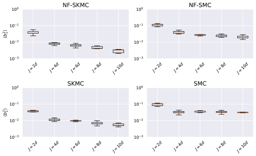
Figure 2: Final dimension averaged squared bias on the first moment for the heat equation model, plotted against the ensemble size $J$ expressed as a multiple of the target dimension $d$.

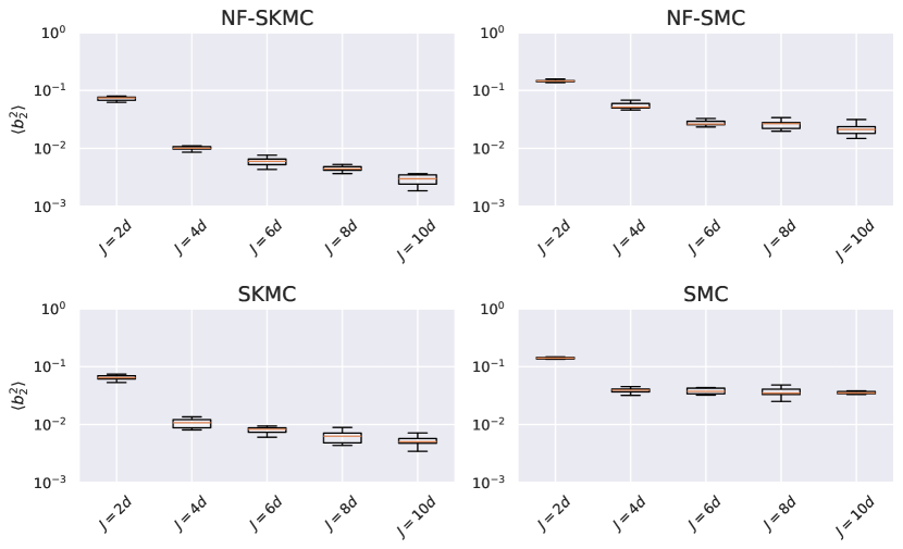
Figure 3: Final dimension averaged squared bias on the second moment for the heat equation model, plotted against the ensemble size $J$ expressed as a multiple of the target dimension $d$.

In Figure 2 we show the results for $\langle b_{1}^{2}\rangle$ obtained with the final particle ensembles for each algorithm, with the box plots showing the variation over the 10 runs. Similarly, Figure 3 shows the results for $\langle b_{2}^{2}\rangle$ obtained for each algorithm. The mean and standard deviation of $\langle b_{1}^{2}\rangle$ and $\langle b_{2}^{2}\rangle$ for each algorithm over their 10 runs are reported in Table 1, alongside the number of temperature levels, $N_{\beta}$ used by each algorithm.

Comparing SKMC with SMC, we can see that SKMC obtains lower values for $\langle b_{1}^{2}\rangle$ and $\langle b_{2}^{2}\rangle$ for all ensemble sizes. The number of temperature levels used by both algorithms is comparable, with SMC requiring additional temperature levels for some random seeds. This is to be expected if the particle ensemble is not sufficiently converged in SMC at each temperature before proceeding to the next temperature level. It is apparent from these tests that SKMC is able to converge more rapidly at each temperature level for this problem, indicating that the EKI update provides a better initialization for the tpCN updates than the importance resampling used in SMC. The EKI update also helps to provide improved preconditioning for the tpCN updates, with the $t$-distribution being fitted to the annealed target particle approximation obtained via the EKI update.

A similar pattern is observed when comparing NF-SKMC and NF-SMC. In comparing each with SKMC and SMC respectively, we see that the improvement from NF preconditioning becomes more pronounced as the ensemble size is increased. For $J=2d$ there are not enough particles for the NF to learn a useful map between between the original data space and a Gaussian latent space. Indeed, in this regime the NF can degrade performance by failing to map to a latent space where the target is effectively Gaussianized, and in the case of NF-SKMC introducing additional non-linearity in the forward model evaluation for the EKI update. For larger ensemble sizes ($J\geq 6d$) the use of NF transformations reduces the final bias for both the NF-SKMC and NF-SMC algorithms. The effect is more pronounced for NF-SKMC, where the NF acts to both relax the Gaussian ansatz of EKI and provide nonlinear preconditioning for the tpCN updates. However, it is worth noting that SKMC was able to achieve low bias without NF preconditioning, demonstrating the potential for the EKI ensemble to initialize and precondition MCMC updates within SMC.

Algorithm	$J$	$N_{\beta}$	$\langle b_{1}^{2}\rangle$	$\langle b_{2}^{2}\rangle$
NF-SKMC	$10d$	$15.0\pm 0.0$	$0.0029\pm 0.0006$	$0.0029\pm 0.0007$
NF-SKMC	$8d$	$15.0\pm 0.0$	$0.0048\pm 0.0008$	$0.0045\pm 0.0005$
NF-SKMC	$6d$	$15.0\pm 0.0$	$0.0065\pm 0.001$	$0.0060\pm 0.001$
NF-SKMC	$4d$	$15.0\pm 0.0$	$0.0084\pm 0.001$	$0.010\pm 0.007$
NF-SKMC	$2d$	$14.8\pm 0.4$	$0.040\pm 0.009$	$0.072\pm 0.006$
SKMC	$10d$	$15.0\pm 0.0$	$0.0056\pm 0.001$	$0.0053\pm 0.001$
SKMC	$8d$	$15.0\pm 0.0$	$0.0071\pm 0.001$	$0.0062\pm 0.001$
SKMC	$6d$	$15.0\pm 0.0$	$0.0094\pm 0.001$	$0.0080\pm 0.001$
SKMC	$4d$	$15.0\pm 0.0$	$0.011\pm 0.002$	$0.011\pm 0.002$
SKMC	$2d$	$15.0\pm 0.0$	$0.038\pm 0.003$	$0.064\pm 0.007$
NF-SMC	$10d$	$15.2\pm 0.4$	$0.021\pm 0.004$	$0.021\pm 0.005$
NF-SMC	$8d$	$15.7\pm 0.5$	$0.025\pm 0.004$	$0.026\pm 0.004$
NF-SMC	$6d$	$15.4\pm 0.5$	$0.029\pm 0.005$	$0.028\pm 0.005$
NF-SMC	$4d$	$15.5\pm 0.5$	$0.041\pm 0.007$	$0.055\pm 0.008$
NF-SMC	$2d$	$14.9\pm 0.3$	$0.11\pm 0.02$	$0.15\pm 0.009$
SMC	$10d$	$15.3\pm 0.5$	$0.032\pm 0.004$	$0.036\pm 0.004$
SMC	$8d$	$15.5\pm 0.5$	$0.034\pm 0.005$	$0.037\pm 0.007$
SMC	$6d$	$15.7\pm 0.5$	$0.036\pm 0.004$	$0.038\pm 0.004$
SMC	$4d$	$15.6\pm 0.5$	$0.033\pm 0.006$	$0.039\pm 0.004$
SMC	$2d$	$15.1\pm 0.3$	$0.094\pm 0.02$	$0.14\pm 0.009$

Table 1: Results for the number of temperature levels used by each algorithm $N_{\beta}$ and squared bias results, $\langle b_{1}^{2}\rangle$ and $\langle b_{2}^{2}\rangle$, obtained with the final particle ensemble for each algorithm when performing inference on the heat equation example. We report the mean and standard deviation for each statistic over the 10 algorithm runs, and show results for each of the tested ensemble sizes $J$. The number of parallelized model evaluations is given by $11N_{\beta}$ for each algorithm, with the total number of model evaluations being given by $11JN_{\beta}$.

3.2 Gravity Survey

For this problem we adapt the $d=2$ gravity surveying problem presented in [63]. We have some mass density field $\varrho(\mbox{\boldmath{$x$}})$, located at a depth $\delta$ from the surface at which measurements of the vertical component of the gravitational field are made. The vertical component of the gravitational field at some point $s$ at the surface is given by

$$\zeta(\mbox{\boldmath{$s$}})=\iint_{X}\frac{\delta}{\left\lVert\mbox{\boldmath{$s$}}-\mbox{\boldmath{$x$}}\right\rVert_{2}^{3}}\varrho(\mbox{\boldmath{$x$}})\mathrm{d}\mbox{\boldmath{$x$}},$$ (46)

where $X=[0,1]^{2}$ is the domain $\varrho(\mbox{\boldmath{$x$}})$. The forward model therefore consists in solving the integral in Equation 46. We follow [63] in evaluating this integral using midpoint quadrature. Using $Q$ quadrature points along each dimension, the integral expression becomes

$$\zeta(\mbox{\boldmath{$s$}}_{i})=\sum_{l=1}^{Q}\omega_{l}\sum_{k=1}^{Q}\omega_{k}\frac{\delta}{\left\lVert\mbox{\boldmath{$s$}}_{i}-\mbox{\boldmath{$x$}}_{k,l}\right\rVert_{2}^{3}}\hat{\varrho}(\mbox{\boldmath{$x$}}_{k,l})=\sum_{j=1}^{Q^{2}}\omega_{j}\frac{\delta}{\left\lVert\mbox{\boldmath{$s$}}_{i}-\mbox{\boldmath{$x$}}_{j}\right\rVert_{2}^{3}}\hat{\varrho}(\mbox{\boldmath{$x$}}_{j}),$$ (47)

where $\omega_{j}=1/Q^{2},\forall j$ are the quadrature weights, $\hat{\varrho}(\mbox{\boldmath{$x$}}_{j})$ is the approximate subsurface density at the quadrature point $\mbox{\boldmath{$x$}}_{j}$, and $\zeta(\mbox{\boldmath{$s$}}_{i}$) is the vertical component of the gravitational field at the collocation point on the surface $\mbox{\boldmath{$s$}}_{i},i\in\{1,\ldots,N^{2}\}$.

The simulated data was obtained by generating a ground truth subsurface density field with profile given by

$$\varrho(\mbox{\boldmath{$x$}})\propto\sin(\pi x_{1})+\sin(3\pi x_{2})+x_{2}+1,\quad x_{1},x_{2}\in[0,1]$$ (48)

normalized to have a maximum value of 1. This signal was projected onto a $64\times 64$ grid. The surface signal was evaluated using Equation 47 on a $10\times 10$ grid, with Gaussian white noise with standard deviation $\sigma_{\eta}=0.1$ being added to each surface pixel to give the simulated data. The true subsurface mass density, and the corresponding surface gravitational field measurements used in this example are shown in Figure 4.

Figure 4: The true subsurface mass density field $\varrho(\mbox{\boldmath{$x$}})$ (left panel), shown alongside the low resolution measurements of the gravitational field at the surface $\zeta(\mbox{\boldmath{$x$}})$ (right panel).

For the inference task we model the subsurface density as a GRF with a Matérn 3/2 covariance kernel,

$$C(\mbox{\boldmath{$x$}},\mbox{\boldmath{$x$}}^{\prime})=\left(1+\frac{\sqrt{3}\left\lVert\mbox{\boldmath{$x$}}-\mbox{\boldmath{$x$}}^{\prime}\right\rVert_{2}}{\ell}\right)\exp\left(-\frac{\sqrt{3}\left\lVert\mbox{\boldmath{$x$}}-\mbox{\boldmath{$x$}}^{\prime}\right\rVert_{2}}{\ell}\right),$$ (49)

where $\ell$ is the correlation length scale. The subsurface density field is parameterized using a KL expansion of the $R=60$ leading eigenmodes,

$$\varrho(\mbox{\boldmath{$x$}})=\mu_{K}+\sigma_{K}\sum_{k=1}^{R=60}\sqrt{\lambda_{k}}\phi_{k}(\mbox{\boldmath{$x$}})\theta_{k},$$ (50)

where $\mu_{K}$ and $\sigma_{K}^{2}$ are the field mean and variance respectively, $\{\lambda_{k}\}_{k=1}^{R=60}$ is a sequence of strictly decreasing, real and positive eigenvalues of the covariance kernel in Equation 49, $\phi_{k}(\mbox{\boldmath{$x$}})$ are the corresponding eigenfunctions of the covariance kernel and $\{\theta_{k}\sim\mathcal{N}(0,1)\}_{k=1}^{R=60}$ are a set of standard Gaussian random variables. Defining $\mbox{\boldmath{$\theta$}}=(\theta_{1},\ldots,\theta_{60})^{\intercal}$, the full model for this example is given by

$$\mu_{K} \sim\mathcal{N}(\mu=0,\sigma^{2}=1^{2}),$$ (51)

$$\sigma_{K} \sim|\mathcal{N}(\mu=0,\sigma^{2}=0.2^{2})|,$$ (52)

$$\theta \sim\mathcal{N}(0,I_{60}),$$ (53)

$$y \sim\mathcal{N}(F_{\zeta}(\mu_{K},\sigma_{K},\mbox{\boldmath{$\theta$}}),\sigma_{\eta}^{2}I_{100})$$ (54)

where $F_{\zeta}(\mu_{K},\sigma_{K},\mbox{\boldmath{$\theta$}})$ denotes the full gravity survey forward model, mapping from the subsurface mass density field to the low resolution surface measurements of the gravitational field $y$. When performing inference a log-transformation is applied to $\sigma_{K}$ such that all parameters are in an unconstrained space, with the target distribution being modified by the corresponding Jacobian.

In Figures 5 and 6 we show the recovered estimates for $\langle b_{1}^{2}\rangle$ and $\langle b_{2}^{2}\rangle$ respectively, with box plots again showing the variation over the 10 runs for each algorithm and ensemble size. The mean and standard deviation for $\langle b_{1}^{2}\rangle$ and $\langle b_{2}^{2}\rangle$, along with the number of temperature levels used by each each algorithm over the 10 runs are reported in Table 2.

Starting with SMC, we can see that the values for $\langle b_{1}^{2}\rangle$ and $\langle b_{2}^{2}\rangle$ are high and largely independent of the ensemble size. In this case, SMC requires significantly more tpCN iterations at each temperature level in order to correctly distribute the particle ensemble after the importance resampling step. In comparison, SKMC is able to achieve a lower bias with the same computational budget being used at each temperature level, albeit not reaching the low bias threshold of $\langle b_{g}^{2}\rangle<10^{-2}$ with 10 tpCN iterations at each temperature level. This indicates that the the particle ensemble obtained by the EKI update provides a better initialization and preconditioner for the tpCN updates compared to the importance resampled particle ensemble, achieving lower bias with fewer model evaluations.

A similar pattern is again observed when comparing the NF-SKMC and NF-SMC algorithms. For larger ensemble sizes the NF is able to map the effective prior at each temperature level to a Gaussian latent space, where the target is approximately Gaussian. For the same computational budget at each temperature level, the NF preconditioning more rapidly distributes particles according to the given target, with the low bias threshold being reached for an ensemble size of $J=10d$ for the NF-SKMC algorithm. For smaller ensemble sizes, the NF is unable to learn useful non-Gaussian features in the geometry of the effective prior, meaning we do not obtain an improvement from NF preconditioning. As with the heat equation, the ability of SKMC to more rapidly converge on the target at each temperature level is indicative of the utility of EKI as an MCMC initialization and preconditioner in regimes where learning effective NF maps is intractable.

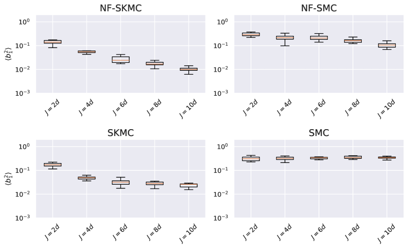
Figure 5: Final dimension averaged squared bias on the first moment for the gravity survey model, plotted against the ensemble size $J$ expressed as a multiple of the target dimension $d$.

Figure 6: Final dimension averaged squared bias on the second moment for the gravity survey model, plotted against the ensemble size $J$ expressed as a multiple of the target dimension $d$.

Algorithm	$J$	$N_{\beta}$	$\langle b_{1}^{2}\rangle$	$\langle b_{2}^{2}\rangle$
NF-SKMC	$10d$	$22.6\pm 0.5$	$0.0098\pm 0.0024$	$0.0089\pm 0.0025$
NF-SKMC	$8d$	$23.0\pm 0.0$	$0.017\pm 0.004$	$0.017\pm 0.003$
NF-SKMC	$6d$	$23.0\pm 0.0$	$0.027\pm 0.009$	$0.025\pm 0.007$
NF-SKMC	$4d$	$23.0\pm 0.0$	$0.058\pm 0.011$	$0.056\pm 0.008$
NF-SKMC	$2d$	$23.2\pm 0.4$	$0.14\pm 0.03$	$0.13\pm 0.02$
SKMC	$10d$	$23.1\pm 0.3$	$0.024\pm 0.005$	$0.022\pm 0.004$
SKMC	$8d$	$23.0\pm 0.0$	$0.028\pm 0.006$	$0.024\pm 0.004$
SKMC	$6d$	$23.2\pm 0.4$	$0.032\pm 0.009$	$0.027\pm 0.008$
SKMC	$4d$	$23.3\pm 0.5$	$0.050\pm 0.010$	$0.049\pm 0.009$
SKMC	$2d$	$23.4\pm 0.5$	$0.17\pm 0.03$	$0.16\pm 0.02$
NF-SMC	$10d$	$23.0\pm 0.0$	$0.11\pm 0.03$	$0.11\pm 0.03$
NF-SMC	$8d$	$23.8\pm 0.4$	$0.17\pm 0.05$	$0.19\pm 0.05$
NF-SMC	$6d$	$24.0\pm 0.0$	$0.22\pm 0.05$	$0.23\pm 0.06$
NF-SMC	$4d$	$24.1\pm 0.3$	$0.22\pm 0.07$	$0.21\pm 0.07$
NF-SMC	$2d$	$23.2\pm 0.3$	$0.31\pm 0.07$	$0.23\pm 0.08$
SMC	$10d$	$23.9\pm 0.3$	$0.35\pm 0.05$	$0.42\pm 0.07$
SMC	$8d$	$24.0\pm 0.0$	$0.35\pm 0.05$	$0.42\pm 0.06$
SMC	$6d$	$24.2\pm 0.4$	$0.34\pm 0.07$	$0.39\pm 0.10$
SMC	$4d$	$24.0\pm 0.6$	$0.31\pm 0.06$	$0.34\pm 0.08$
SMC	$2d$	$23.5\pm 0.5$	$0.32\pm 0.07$	$0.25\pm 0.06$

Table 2: Results for the number of temperature levels used by each algorithm $N_{\beta}$ and squared bias results, $\langle b_{1}^{2}\rangle$ and $\langle b_{2}^{2}\rangle$, obtained with the final particle ensemble for each algorithm, when performing inference on the gravity survey example. We report the mean and standard deviation for each statistic over the 10 algorithm runs, and show results for each of the tested ensemble sizes $J$. The number of parallelized model evaluations is given by $11N_{\beta}$ for each algorithm, with the total number of model evaluations being given by $11JN_{\beta}$.

3.3 Reaction-Diffusion Equation

We consider a reaction-diffusion system in one spatial dimension, where some quantity $s(x,t)$ varies with time under the action of some source term $u(x)$. This time evolution is described by a nonlinear reaction-diffusion equation of the form

$$\frac{\partial s(x,t)}{\partial t}=D\frac{\partial^{2}s(x,t)}{\partial x^{2}}+\gamma s^{2}(x,t)+u(x),\quad x\in\Omega=[0,1],$$ (55)

where $D=0.1$ is the diffusion constant and $\gamma=0.1$ is the reaction rate. For this problem, we study the recovery of the source function $u(x)$ from observations of $s(x,t)$. To solve Equation 55 we use the implicit, second-order finite difference scheme implemented in [64]. We assume Dirichlet boundary conditions such that $s(x,t)=0,\forall x\in\partial\Omega$, and the initial condition $s(x,t=0)=0$. The solution to Equation 55 is evaluated on a $100\times 100$ grid in $(x,t)$, up to a final time $t_{f}=1$.

We parameterize the source term using the Hilbert space expansion of a Gaussian Process (GP) [65] with a squared exponential kernel,

$$u(x)=\mu_{H}+\sum_{j=1}^{R}\left[S_{\Theta}\left(\sqrt{\lambda_{j}}\right)\right]^{1/2}\phi_{j}(x)\theta_{j},$$ (56)

where $\mu_{H}$ is the Hilbert space GP mean, $S_{\Theta}(\omega)=\alpha_{H}\sqrt{2\pi}\ell_{H}\exp(-\ell^{2}_{H}\omega^{2}/2)$ is the squared exponential kernel spectral density function, $\Theta=(\alpha_{H},\ell_{H})$ denotes the kernel hyperparmeters i.e., the kernel variance $\alpha_{H}$ and length scale $\ell_{H}$, $\{\lambda_{j}\}_{j=1}^{\infty}$ and $\{\phi_{j}(x)\}_{j=1}^{\infty}$ are the eigenvalues and eigenfunctions of the Laplacian operator on some domain $\Omega_{L}=[-L,L]$ respectively, and $\theta_{j}\sim\mathcal{N}(0,1)$ are a set of standard Gaussian random variables. The eigenvalues and eigenfunctions of the Laplacian operator are given by

$$\lambda_{j} =\left(\frac{j\pi}{2L}\right)^{2},$$ (57)

$$\phi_{j}(x) =\sqrt{\frac{1}{L}}\sin\left(\sqrt{\lambda_{j}}(x+L)\right).$$ (58)

Without loss of generality, we can evaluate $u(x)$ on the symmetric interval $[-0.5,0.5]$, choosing the domain for the Laplacian operator $\Omega_{L}=[-1,1]$ such that it contains the full spatial domain of $u(x)$ [65].

To generate a simulated data set, we obtain a realisation of $u(x)$ from Equation 56 with $\mu_{H}=0$, $\alpha_{H}=1$ and $\ell_{H}=0.1$. We solve for $s(x,t)$ subject to the corresponding Dirichlet boundary conditions, up to a time $t_{f}=1$ on the $100\times 100$ grid in $(x,t)$. The field $s(x,t)$ is then observed at 10 equally spaced spatial locations, at 10 equally spaced times, with Gaussian observation noise corresponding to a noise standard deviation of $\sigma_{\eta}=0.01$. The true source function is shown in Figure 7, alongside the corresponding solution for $s(x,t)$ and the locations of the $s(x,t)$ measurements.

Figure 7: The true source term $u(x)$ (left panel), shown alongside the corresponding solution for $s(x,t)$ (right panel). White circles on the right panel denote the locations where measurements of $s(x,t)$ were made.

For the inference task here we consider recovering the first $R=50$ terms in the Hilbert space expansion. Denoting $\mbox{\boldmath{$\theta$}}=(\theta_{1},\ldots,\theta_{50})^{\intercal}$, the full model is given by

$$\mu_{H} \sim\mathcal{N}(\mu=0,\sigma^{2}=0.1^{2}),$$ (59)

$$\alpha_{H} \sim|\mathcal{N}(\mu=0,\sigma^{2}=1^{2})|,$$ (60)

$$\ell_{H} \sim\mathrm{InverseGamma}(\alpha=4,\beta=0.3),$$ (61)

$$\theta \sim\mathcal{N}(0,I_{50}),$$ (62)

$$y \sim\mathcal{N}(F_{RD}(\mu_{H},\alpha_{H},\ell_{H},\mbox{\boldmath{$\theta$}}),\sigma_{\eta}^{2}I_{100}),$$ (63)

where $F_{RD}(\mu_{H},\alpha_{H},\ell_{H},\mbox{\boldmath{$\theta$}})$ denotes the full forward model, mapping from the source function $u(x)$ to the $s(x,t)$ observations $y$. When running our set of inference algorithms, we apply log-transformations to $\alpha_{H}$ and $\ell_{H}$ such that all parameters are mapped to an unconstrained space, making the corresponding Jacobian adjustments to the target.

In Figures 8 and 9 we show the recovered estimates for $\langle b_{1}^{2}\rangle$ and $\langle b_{2}^{2}\rangle$ respectively, with box plots showing the variation over the 10 runs for each algorithm and ensemble size. In Table 3 we report the mean and standard deviation for $\langle b_{1}^{2}\rangle$ and $\langle b_{2}^{2}\rangle$, along with the mean and standard deviation on the number of temperature levels used by each algorithm over the 10 runs.

Figure 8: Final dimension averaged squared bias on the first moment for the reaction-diffusion model, plotted against the ensemble size $J$ expressed as a multiple of the target dimension $d$.

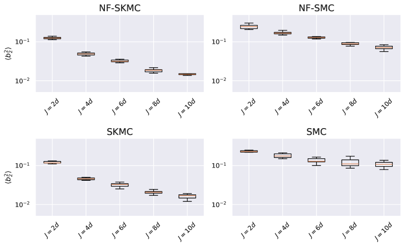
Figure 9: Final dimension averaged squared bias on the second moment for the reaction-diffusion model, plotted against the ensemble size $J$ expressed as a multiple of the target dimension $d$.

Algorithm	$J$	$N_{\beta}$	$\langle b_{1}^{2}\rangle$	$\langle b_{2}^{2}\rangle$
NF-SKMC	$10d$	$17.0\pm 0.0$	$0.017\pm 0.002$	$0.015\pm 0.002$
NF-SKMC	$8d$	$17.0\pm 0.0$	$0.018\pm 0.003$	$0.018\pm 0.002$
NF-SKMC	$6d$	$17.8\pm 0.4$	$0.029\pm 0.004$	$0.032\pm 0.002$
NF-SKMC	$4d$	$18.0\pm 0.0$	$0.040\pm 0.010$	$0.049\pm 0.004$
NF-SKMC	$2d$	$19.1\pm 0.3$	$0.076\pm 0.016$	$0.13\pm 0.01$
SKMC	$10d$	$17.0\pm 0.0$	$0.020\pm 0.003$	$0.016\pm 0.002$
SKMC	$8d$	$17.1\pm 0.3$	$0.028\pm 0.004$	$0.021\pm 0.002$
SKMC	$6d$	$17.6\pm 0.5$	$0.033\pm 0.007$	$0.032\pm 0.004$
SKMC	$4d$	$18.0\pm 0.0$	$0.038\pm 0.004$	$0.046\pm 0.003$
SKMC	$2d$	$19.0\pm 0.4$	$0.072\pm 0.013$	$0.12\pm 0.007$
NF-SMC	$10d$	$18.0\pm 0.0$	$0.072\pm 0.007$	$0.072\pm 0.008$
NF-SMC	$8d$	$18.6\pm 0.5$	$0.084\pm 0.010$	$0.093\pm 0.015$
NF-SMC	$6d$	$19.0\pm 0.0$	$0.11\pm 0.009$	$0.13\pm 0.01$
NF-SMC	$4d$	$19.8\pm 0.4$	$0.14\pm 0.02$	$0.18\pm 0.03$
NF-SMC	$2d$	$21.3\pm 0.5$	$0.21\pm 0.02$	$0.25\pm 0.03$
SMC	$10d$	$18.0\pm 0.0$	$0.11\pm 0.01$	$0.11\pm 0.02$
SMC	$8d$	$18.1\pm 0.3$	$0.13\pm 0.03$	$0.12\pm 0.03$
SMC	$6d$	$18.9\pm 0.3$	$0.13\pm 0.02$	$0.13\pm 0.02$
SMC	$4d$	$19.5\pm 0.5$	$0.15\pm 0.01$	$0.18\pm 0.02$
SMC	$2d$	$21.1\pm 0.5$	$0.20\pm 0.04$	$0.24\pm 0.07$

Table 3: Results for the number of temperature levels used by each algorithm $N_{\beta}$ and squared bias results, $\langle b_{1}^{2}\rangle$ and $\langle b_{2}^{2}\rangle$, obtained with the final particle ensemble for each algorithm, when performing inference on the reaction-diffusion example. We report the mean and standard deviation for each statistic over the 10 algorithm runs, and show results for each of the tested ensemble sizes $J$. The number of parallelized model evaluations is given by $11N_{\beta}$ for each algorithm, with the total number of model evaluations being given by $11JN_{\beta}$.

Comparing SKMC with SMC, we can see that SKMC is able to achieve significantly lower bias with the final particle ensemble using the same computational budget at each temperature level. This again indicates the the SKMC update provides a better initialization and preconditioner for the subsequent tpCN iteration than the importance resampled ensemble in SMC. For this problem, we only obtain a small improvement in the final bias with NF preconditioning for larger ensemble sizes ($J\geq 6d$). The target posterior for this problem is close to Gaussian, meaning the NF map does not introduce a latent space where the target geometry is such that sampling is significantly easier. In all cases for this example the final ensemble did not reach the low bias threshold ($\langle b_{g}^{2}\rangle<0.01$). To do so would require additional tpCN iterations at each temperature level. An appropriate number of tpCN iterations could be selected using an adaptive scheme e.g., by monitoring the correlation between the initial particle ensemble and the current particle ensemble at each temperature level. We leave a detailed analysis of fully adaptive variants of SKMC and NF-SKMC to future work, where we plan to implement the algorithms within the pocoMC sampling package [35, 54].

4 Conclusions

In this work we have considered the problem of performing Bayesian inference on inverse problems where the forward model is expensive to evaluate and we do not have access to derivatives of the forward model. In such a situation, standard sampling methods such as MCMC and SMC algorithms can quickly become intractable, requiring a large number of serial model evaluations to attain low bias estimates of posterior moments [16]. In contrast, EKI methods have been proposed that can rapidly converge on an ensemble approximation to the target posterior. However, these methods are derived on the assumption that the forward model is linear and that we progress through a sequence of Gaussian measures in moving from the prior to the posterior. Outside of this regime, the EKI ensemble is an uncontrolled approximation to the posterior. Whilst EKI often shows good empirical performance outside of the linear, Gaussian regime, particularly in optimizing for point estimates of model parameters, this is insufficient for many scientific inference tasks where we seek accurate uncertainty estimates and hence low bias estimates for higher order posterior moments.

In this work, we proposed integrating EKI updates within an SMC framework, replacing the standard importance resampling step at each temperature level with an EKI update. This was designed to both correct for the assumptions inherent to EKI, and to accelerate SMC with the EKI target approximations. We considered two variants of the Sequential Kalman Monte Carlo (SKMC) algorithms, the standard SKMC algorithm, and the NF-SKMC algorithm detailed in Algorithm 1 where NF preconditioning is used to both relax the Gaussian ansatz of EKI and to improve the performance of the sampling iterations performed at each temperature level. For the sampling iterations we use the $t$-preconditioned Crank-Nicolson (tpCN) algorithm. The tpCN proposal kernel is reversible with respect to the multivariate $t$-distribution, which enables more efficient sampling of heavy tailed targets. When performing sampling in the NF latent space we have an effective double preconditioning, with the NF mapping the effective prior to a Gaussian latent space, and the tpCN proposal accounting for any residual tails in the annealed latent space target.

We compared the performance of the SKMC and NF-SKMC samplers with standard importance resampling SMC and NF-SMC, running each algorithm on three inverse problems. For the first problem we considered recovering some initial temperature field from low resolution measurements of the temperature field at some later time, evolving under the heat equation. In the second problem we studied the recovery of an underlying density field given surface measurements of the gravitational field, and in the third problem we inferred a source function driving a signal evolving under the reaction-diffusion equation.

For all the numerical experiments, the SKMC and NF-SKMC samplers were able to attain a lower bias on estimates for the first and second posterior moments, compared to the SMC and NF-SMC samplers using the same computational budget at each temperature level. It is worth noting that the SKMC sampler was able to achieve a lower bias than the NF-SMC sampler, demonstrating the ability of the EKI ensemble update to provide an effective initialization and preconditioner for the subsequent sampling steps. This is particularly promising for regimes where learning high fidelity NF maps becomes intractable e.g., moving beyond $\mathcal{O}(100)$ dimensions, or where one wishes to avoid the additional computational overhead from NF training.

For the heat equation and gravity survey examples, the NF-SKMC sampler was able to achieve noticeably lower bias for larger ensemble sizes, with the same computational budget at each temperature level (and approximately the same total computational budget given the small variations in the number of temperature levels used). For smaller ensemble sizes ($J=4d$ and $J=2d$), there was not enough information for the NF to learn an effective map from the effective prior to a Gaussian latent space. For the reaction-diffusion example, the target posterior and intermediate target measures were close to Gaussian. Learning NF maps to a Gaussian latent space at each temperature level therefore did not significantly improve the final bias on estimates of the posterior moments. NF preconditioning is primarily useful for inverse problems where the cost of NF training (of order seconds in our examples), is insignificant compared to the cost of forward model evaluations and where one can afford ensemble sizes that are sufficiently large to learn nonlinear features in the target geometry.

Several avenues exist for extending this work. In the first instance we plan to incorporate the SKMC and NF-SKMC samplers within the pocoMC sampling package [35, 54], which currently implements adaptive variants of SMC and NF-SMC. In tandem with this, we will explore fully adaptive variants of the SKMC and NF-SKMC algorithms, with the goal of reliably attaining low bias posterior representations through the final particle ensemble. For example, in our three examples using 10 tpCN iterations at each temperature level was often insufficient for reaching the low bias regime. It would therefore be useful to establish robust criteria for selecting the number of tpCN iterations at each temperature level. It would also be interesting to explore alternative NF architectures that are able to learn useful features in the target geometry with smaller ensemble sizes [39], and waste-free SMC methods that allow us to exploit the full sampling history in the SMC framework [34]. In this work we have only considered one variant of the EKI-type updates within SMC. It would be worth studying the performance of alternative ensemble updates e.g., deterministic square root inversion methods [14], Ensemble Adjustment Kalman Inversion, Ensemble Transform Kalman Inversion [16], etc. These deterministic updates have been shown to have superior empirical performance compared to the stochastic EKI update used in this work [16]. In addition to studying the application of deterministic Kalman updates, it would be useful to consider extensions allowing for parameter dependent noise covariances [66] and general likelihoods [67].

Appendix A Proof of Lemma 2.1

Proof.

Consider the current location $x$ and the proposal location $\mbox{\boldmath{$x$}}^{\prime}=\mbox{\boldmath{$\mu$}}_{s}+\sqrt{1-\rho^{2}}(\mbox{\boldmath{$x$}}-\mbox{\boldmath{$\mu$}}_{s})+\rho\sqrt{Z}\mbox{\boldmath{$W$}}$, where $Z^{-1}\sim\mathrm{Gamma}(k=\frac{1}{2}(d+\nu_{s}),\theta=2/(\nu_{s}+\langle\mbox{\boldmath{$x$}},\mbox{\boldmath{$x$}}\rangle_{s}))$ and $\mbox{\boldmath{$W$}}\sim\mathcal{N}(0,\mathcal{C}_{s})$.

We have that

$$\sqrt{\frac{(d+\nu_{s})Z}{\nu_{s}+\langle\mbox{\boldmath{$x$}},\mbox{\boldmath{$x$}}\rangle_{s}}}\mbox{\boldmath{$W$}}\sim t_{d+\nu_{s}}(0,\mathcal{C}_{s}).$$ (64)

Using the change of variables formula, we obtain the proposal transition kernel for the tpCN algorithm as

$$\mathcal{K}_{t}(\mbox{\boldmath{$x$}},\mathrm{d}\mbox{\boldmath{$x$}}^{\prime})=\frac{\gamma_{1}}{\rho^{d}}\left(\frac{d+\nu_{s}}{\nu_{s}+\langle\mbox{\boldmath{$x$}},\mbox{\boldmath{$x$}}\rangle_{s}}\right)^{d/2}\left[1+\right.\\ \left.(\rho^{2}(\nu_{s}+\langle\mbox{\boldmath{$x$}},\mbox{\boldmath{$x$}}\rangle_{s}))^{-1}(\langle\mbox{\boldmath{$x$}}^{\prime},\mbox{\boldmath{$x$}}^{\prime}\rangle_{s}+(1-\rho^{2})\langle\mbox{\boldmath{$x$}},\mbox{\boldmath{$x$}}\rangle_{s}-2\sqrt{1-\rho^{2}}\langle\mbox{\boldmath{$x$}},\mbox{\boldmath{$x$}}^{\prime}\rangle_{s})\right]^{-(2d+\nu_{s})/2}\mathrm{d}\mbox{\boldmath{$x$}}^{\prime},$$ (65)

where $\gamma_{1}$ is a normalizing constant. Considering the multivariate $t$-measure

$$p_{s}(\mathrm{d}\mbox{\boldmath{$x$}})=\gamma_{2}\left[1+\frac{\langle\mbox{\boldmath{$x$}},\mbox{\boldmath{$x$}}\rangle_{s}}{\nu_{s}}\right]^{-(d+\nu_{s})/2}\mathrm{d}\mbox{\boldmath{$x$}},$$ (66)

where $\gamma_{2}$ is a normalizing constant, we have that

$$p_{s}(\mathrm{d}\mbox{\boldmath{$x$}})\mathcal{K}_{t}(\mbox{\boldmath{$x$}},\mathrm{d}\mbox{\boldmath{$x$}}^{\prime})=\gamma_{1}\gamma_{2}\nu_{s}^{(d+\nu_{s})/2}(d+\nu_{s})^{d/2}\rho^{d+\nu_{s}}\left[\rho^{2}\nu_{s}+\langle\mbox{\boldmath{$x$}}^{\prime},\mbox{\boldmath{$x$}}^{\prime}\rangle_{s}+\langle\mbox{\boldmath{$x$}},\mbox{\boldmath{$x$}}\rangle_{s}\right.\\ \left.-2\sqrt{1-\rho^{2}}\langle\mbox{\boldmath{$x$}},\mbox{\boldmath{$x$}}^{\prime}\rangle_{s}\right]^{-(2d+\nu_{s})/2}\mathrm{d}\mbox{\boldmath{$x$}}\mathrm{d}\mbox{\boldmath{$x$}}^{\prime}=p_{s}(\mathrm{d}\mbox{\boldmath{$x$}}^{\prime})\mathcal{K}_{t}(\mbox{\boldmath{$x$}}^{\prime},\mathrm{d}\mbox{\boldmath{$x$}}).$$ (67)

The variables $x$ and $\mbox{\boldmath{$x$}}^{\prime}$ are exchangeable in Equation 67. Therefore the tpCN proposal transition kernel is reversible with respect to the multivariate $t$-distribution $t_{\nu_{s}}(\mbox{\boldmath{$\mu$}}_{s},\mathcal{C}_{s})$.

The tpCN acceptance probability follows from the fact that for some general proposal kernel, $\mathcal{K}(\mbox{\boldmath{$x$}},\mathrm{d}\mbox{\boldmath{$x$}}^{\prime})$ with probability density function $\kappa(\mbox{\boldmath{$x$}},\mbox{\boldmath{$x$}}^{\prime})$, the Metropolis-Hastings (MH) acceptance probability is given by

$$\alpha(\mbox{\boldmath{$x$}},\mbox{\boldmath{$x$}}^{\prime})=\mathrm{min}\left\{1,\frac{p(\mbox{\boldmath{$x$}}^{\prime})\kappa(\mbox{\boldmath{$x$}}^{\prime},\mbox{\boldmath{$x$}})}{p(\mbox{\boldmath{$x$}})\kappa(\mbox{\boldmath{$x$}},\mbox{\boldmath{$x$}}^{\prime})}\right\}.$$ (68)

From the reversibility expression in Equation 67 we have that

$$\frac{\kappa_{t}(\mbox{\boldmath{$x$}}^{\prime},\mbox{\boldmath{$x$}})}{\kappa_{t}(\mbox{\boldmath{$x$}},\mbox{\boldmath{$x$}}^{\prime})}=\frac{p_{s}(\mbox{\boldmath{$x$}})}{p_{s}(\mbox{\boldmath{$x$}}^{\prime})}=\frac{(1+\langle\mbox{\boldmath{$x$}},\mbox{\boldmath{$x$}}\rangle_{s}/\nu_{s})^{-(d+\nu_{s})/2}}{(1+\langle\mbox{\boldmath{$x$}}^{\prime},\mbox{\boldmath{$x$}}^{\prime}\rangle_{s}/\nu_{s})^{-(d+\nu_{s})/2}},$$ (69)

which gives the MH acceptance probability in Equation 31. ∎

Appendix B Importance Resampling

Given a set of samples and associated normalized importance weights $\left\{\mbox{\boldmath{$x$}}^{i}_{n},\tilde{w}_{n}(\mbox{\boldmath{$x$}}^{i}_{n})\right\}_{i=1}^{J}$, where $\tilde{w}_{n}(\mbox{\boldmath{$x$}}_{n}^{i})=w_{n}(\mbox{\boldmath{$x$}}_{n}^{i})/\sum_{k=1}^{J}w_{n}(\mbox{\boldmath{$x$}}_{n}^{k})$, we can apply a resampling algorithm to obtain a set of equal weight samples. A simple approach would be to apply multinomial resampling, where the duplication counts for each member of the ensemble $\{N^{1},\ldots,N^{J}\}$ are obtained by sampling from the multinomial distribution $\mathrm{Mult}(J;\tilde{w}_{n}(\mbox{\boldmath{$x$}}_{n}^{1}),\ldots,\tilde{w}_{n}(\mbox{\boldmath{$x$}}_{n}^{J}))$. Whilst multinomial resampling is straightforward, lower variance methods are available [42]. In this work we use systematic resampling for all our importance resampling SMC benchmarks. The systematic resampling algorithm pseudocode is given in Algorithm 2.

Algorithm 2 Systematic Resampling

1:  Input: Set of $J$ samples and corresponding normalized importance weights $\{\mbox{\boldmath{$x$}}^{i},\tilde{w}^{i}\}_{i=1}^{J}$.

2:  Draw uniform random variable $U\sim\mathrm{Unif}(0,1)$.

3:  Set $U^{i}=U+(i-1)/J$, $i\in\{1,\ldots,J\}$.

4:  Set $D_{w}=\tilde{w}^{0}$.

5:  Set index counter $k=1$

6:  for $i=1,\ldots,J$ do

7:     while $U^{i}>D_{w}$ do

8:        $k\leftarrow k+1$

9:        $D_{w}\leftarrow D_{w}+\tilde{w}^{k}$

10:     end while

11:     Set $\tilde{\mbox{\boldmath{$x$}}^{i}}=\mbox{\boldmath{$x$}}^{k}$.

12:  end for

13:  Output: Equal weight particle ensemble $\{\tilde{\mbox{\boldmath{$x$}}}^{i}\}_{i=1}^{J}$.

Appendix C Sequential Monte Carlo Implementations

In Algorithm 3 we give the pseudocode for the normalizing flow preconditioned SMC implementation, used as a benchmark for comparing the performance of the SKMC samplers. The SMC implementation without NF preconditioning follows the same structure as Algorithm 3, without the NF fits such that the tpCN iterations are performed in the original data space. Similarly to the SKMC samplers, we perform diminishing adaptation of the tpCN step size and reference measure mean at each temperature level.

Algorithm 3 Flow Preconditioned Sequential Monte Carlo

1:  Input: Set of $J$ samples from the prior $\{\mbox{\boldmath{$x$}}_{0}^{i}\sim\pi_{0}(\mbox{\boldmath{$x$}})\}_{i=1}^{J}$, data $y$, observation covariance $\Gamma$, target fractional ESS $\tau$, number of tpCN iterations to perform at each temperature level $M$, initial tpCN step size $\rho$, target tpCN acceptance rate $\alpha^{\star}$.

2:  Set $\beta_{0}=0$ and iteration counter $n=0$.

3:  while $\beta_{n}<1$  do

4:     Solve for target inverse temperature $\beta_{n+1}$ in Equation 19.

5:     $w_{n}(\mbox{\boldmath{$x$}}_{n}^{i})\leftarrow\pi(\mbox{\boldmath{$y$}}|\mbox{\boldmath{$x$}}_{n}^{i})^{\beta_{n+1}}/\pi(\mbox{\boldmath{$y$}}|\mbox{\boldmath{$x$}}_{n}^{i})^{\beta_{n}},\quad i\in\{1,\ldots,J\}$.

6:     if $\beta_{n+1}=1$ then

7:        $n^{*}\leftarrow n+1$

8:     end if

9:     Fit NF map, $\mbox{\boldmath{$z$}}=f_{n}(\mbox{\boldmath{$x$}})$ to current particle locations $\{\mbox{\boldmath{$x$}}_{n}^{i}\}_{i=1}^{J}$.

10:     Obtain latent space particle locations $\{\mbox{\boldmath{$z$}}_{n}^{i}=f_{n}(\mbox{\boldmath{$x$}}_{n}^{i})\}_{i=1}^{J}$.

11:     Resample weighted particles $\{\mbox{\boldmath{$z$}}_{n}^{i},w_{n}(\mbox{\boldmath{$x$}}_{n}^{i}=f_{n}^{-1}(\mbox{\boldmath{$z$}}_{n}^{i}))\}$ using systematic resampling to give equal weight ensemble $\{\mbox{\boldmath{$z$}}_{n+1}^{i}\}_{i=1}^{J}$.

12:     Fit the multivariate $t$-distribution, $t_{\nu_{s}}(\mu_{s},\mathcal{C}_{s})$ to the latent space particle ensemble $\{\mbox{\boldmath{$z$}}^{i}_{n+1}\}_{i=1}^{J}$ with an EM algorithm.

13:     for $m=1,\ldots,M$ do

14:        for $i=1,\ldots,J$ do

15:           Draw $1/Z_{m}^{i}\sim\mathrm{Gamma}\left(\frac{(d+\nu_{s})}{2},\frac{2}{\nu_{s}+\langle\mbox{\boldmath{$z$}}_{n+1},\mbox{\boldmath{$z$}}_{n+1}\rangle_{s}}\right)$, and $\mbox{\boldmath{$W$}}_{m}^{i}\sim\mathcal{N}(0,\mathcal{C}_{s})$.

16:           $\mbox{\boldmath{$z$}}_{n+1}^{i^{\prime}}\leftarrow\mbox{\boldmath{$\mu_{s}$}}+\sqrt{1-\rho^{2}}(\mbox{\boldmath{$z$}}_{n+1}^{i}-\mbox{\boldmath{$\mu$}}_{s})+\rho\sqrt{Z_{m}^{i}}\mbox{\boldmath{$W$}}_{m}^{i}$

17:           Update particle with probability $\alpha(\mbox{\boldmath{$z$}}_{n+1}^{i},\mbox{\boldmath{$z$}}_{n+1}^{i^{\prime}})$, such that

$$\mbox{\boldmath{$z$}}_{n+1}^{i}=\begin{cases}\mbox{\boldmath{$z$}}_{n+1}^{i^{\prime}}&\text{with probability}\>\alpha(\mbox{\boldmath{$z$}}_{n+1}^{i},\mbox{\boldmath{$z$}}_{n+1}^{i^{\prime}}),\\ \mbox{\boldmath{$z$}}_{n+1}^{i}&\text{with probability}\>1-\alpha(\mbox{\boldmath{$z$}}_{n+1}^{i},\mbox{\boldmath{$z$}}_{n+1}^{i^{\prime}}),\end{cases}$$ (70)

where $\alpha(\mbox{\boldmath{$z$}}_{n+1}^{i},\mbox{\boldmath{$z$}}_{n+1}^{i^{\prime}})$ is given by Equation 32.

18:        end for

19:        $\log\rho\leftarrow\log\rho+(\langle\alpha\rangle-\alpha^{\star})/m$

20:        $\mbox{\boldmath{$\mu$}}_{s}\leftarrow\mbox{\boldmath{$\mu$}}_{s}+(\langle\mbox{\boldmath{$z$}}_{n+1}\rangle-\mbox{\boldmath{$\mu_{s}$}})/m$

21:     end for

22:     Map particle ensemble back to the original data space $\{\mbox{\boldmath{$x$}}_{n+1}^{i}=f^{-1}_{n}(\mbox{\boldmath{$z$}}_{n+1}^{i})\}_{i=1}^{J}$

23:     $n\leftarrow n+1$

24:  end while

25:  Output: Converged particle ensemble $\{\mbox{\boldmath{$x$}}_{n^{*}}^{i}\}_{i=1}^{J}$.

Appendix D Field and Source Term Reconstructions

In Figure 10 we show the true initial temperature field from the heat equation example in Section 3.1, alongside the reconstructed initial field from HMC samples, and the field reconstructions obtained by evaluating the average over the final particle ensembles for each of the NF-SKMC, NF-SMC, SKMC and SMC algorithms, for a single random seed initialization with an ensemble size $J=10d$. In Figure 11 we similarly show the true subsurface density field for the gravity survey example in Section 3.2, alongside the reconstructed subsurface density fields obtained with HMC samples and each of the NF-SKMC, NF-SMC, SKMC and SMC algorithms. In Figure 12 we show the true source function, $u(x)$ for the reaction-diffusion example in Section 3.3, alongside posterior predictive samples for $u(x)$ obtained using HMC and each of the NF-SKMC, NF-SMC, SKMC and SMC algorithms.

For each of the examples considered in this work the qualitative reconstruction of the initial fields and source terms was largely comparable to the recovery with HMC, which is treated as the ground truth representation of the posterior. However, the ability of each method to obtain comparable field and source term recoveries does not fully reflect the ability of the various algorithms in accurately approximating marginal posterior moments. This is captured by the squared-bias statistics reported in this work, which demonstrate the ability to of the SKMC samplers to obtain lower bias and hence better uncertainty quantification compared to importance-resampled SMC.

Figure 10: True initial temperature field $u(\mbox{\boldmath{$x$}},t=0)$ for the heat equation example (Section 3.1), plotted alongside the initial field reconstructions obtained using samples from HMC, which is treated as the target posterior predictive mean, and from the final particle ensembles of the NF-SKMC, NF-SMC, SKMC and SMC algorithms (where results are shown for an ensemble size $J=10d$, and for a single random seed initialization).

Figure 11: True subsurface mass density field $\varrho(\mbox{\boldmath{$x$}})$ for the gravity survey example (Section 3.2), plotted alongside the density field reconstructions obtained using samples from HMC, which is treated as the target posterior predictive mean, and from the final particle ensembles of the NF-SKMC, NF-SMC, SKMC and SMC algorithms (where results are shown for an ensemble size $J=10d$, and for a single random seed initialization).

Figure 12: True source function $u(x)$ for the reaction-diffusion example (Section 3.3), plotted alongside posterior predictive samples obtained with HMC, which are treated as true posterior predictive samples, and from the final particle ensembles of the NF-SKMC, NF-SMC, SKMC and SMC algorithms (where results are shown for an ensemble size $J=10d$, and for a single random seed initialization). For each algorithm we show 100 posterior predictive samples, with the dark red line showing the estimated posterior predictive mean in each case.

Appendix E Flow Annealed Kalman Inversion and Ensemble Kalman Inversion Ablation

In Figures 13, 14 and 15 we show corner plots of the recovered particle distributions from running EKI and FAKI on the heat equation, gravity survey and reaction-diffusion examples respectively. For all plots we also show the sample distributions from our reference HMC samples. We use an ensemble size of $J=10d$ throughout for EKI and FAKI, and show the particle distributions over the first 4 dimensions for illustrative purposes.

From these corner plots, we can immediately see that the particle distributions from EKI and FAKI are strongly offset from the reference HMC sample distributions, meaning any posterior moment estimates obtained from EKI and FAKI will be highly biased. For our numerical examples, we break the core assumptions underlying EKI. This means that in moving from the prior to the first annealed target, the updated ensemble will not be correctly distributed according to the annealed target. When updating the particles for the next temperature level, we do not have the correct effective prior ensemble, meaning these errors will accumulate as we move from the prior to the posterior. For FAKI, we still have these problems, given that the NF maps do not address any errors arising due to nonlinearity. If the particle ensemble is not correctly distributed at a given temperature level, the NF will not Gaussianize the correct effective prior, meaning we lose the additional benefits from mapping the particle ensemble to a Gaussian latent space at each iteration. These results all demonstrate the importance of using the sampling iterations in SMC to correct the EKI and FAKI updates in order to obtain reliable estimates for posterior moments.

Figure 13: Corner plots showing the final particle ensemble for the first 5 dimensions, obtained using EKI (left panel) and FAKI (right panel), plotted alongside reference HMC samples for the heat equation example.

Figure 14: Corner plots showing the final particle ensemble for the first 4 dimensions, obtained using EKI (left panel) and FAKI (right panel), plotted alongside reference HMC samples for the gravity survey example.

Figure 15: Corner plots showing the final particle ensemble for the first 4 dimensions, obtained using EKI (left panel) and FAKI (right panel), plotted alongside reference HMC samples for the reaction-diffusion example.

References

References

- [1] Kaipio J and Somersalo E 2005 Statistical and Computational Inverse Problems (Springer)
- [2] MacKay D J C 2003 Information theory, inference, and learning algorithms (Cambridge University Press)
- [3] Lewis A and Bridle S 2002 Physical Review D 66 103511
- [4] Blas D, Lesgourgues J and Tram T 2011 Journal of Cosmology and Astroparticle Physics 2011 034
- [5] Jasak H, Jemcov A and Tukovic Z 2007 Openfoam: A c++ library for complex physics simulations International workshop on coupled methods in numerical dynamics, volume 1000, pages 1–20. IUC Dubrovnik Croatia
- [6] Tan Z, Kaul C M, Pressel K G, Cohen Y, Schneider T and Teixeira J 2018 Journal of Advances in Modeling Earth Systems 10 770–800
- [7] Iglesias M A, Law K J and Stuart A M 2013 Inverse Problems 29 045001
- [8] Iglesias M A 2016 Inverse Problems 32 025002
- [9] Iglesias M, Park M and Tretyakov M 2018 Inverse Problems 34 105002
- [10] Chada N K, Iglesias M A, Roininen L and Stuart A M 2018 Inverse Problems 34 055009
- [11] Kovachki N B and Stuart A M 2019 Inverse Problems 35 095005
- [12] Chada N K, Stuart A M and Tong X T 2020 SIAM Journal on Numerical Analysis 58 1263–1294
- [13] Iglesias M and Yang Y 2021 Inverse Problems 37 025008
- [14] Ding Z, Li Q and Lu J 2021 Foundations of Data Science 3 371–411
- [15] Huang D Z, Schneider T and Stuart A M 2022 Journal of Computational Physics 463 111262
- [16] Huang D Z, Huang J, Reich S and Stuart A M 2022 Inverse Problems 38 125006
- [17] Chada N and Tong X 2022 Mathematics of Computation 91 1247–1280
- [18] Grumitt R D P, Karamanis M and Seljak U 2024 Flow annealed kalman inversion for gradient-free inference in bayesian inverse problems Physical Sciences Forum vol 9 (MDPI) p 21
- [19] Geyer C J 1992 Statistical Science 7 473–483 ISSN 08834237
- [20] Gelman A, Gilks W R and Roberts G O 1997 The Annals of Applied Probability 7 110 – 120
- [21] Neal R M et al. 2011 Handbook of Markov Chain Monte Carlo 2 2
- [22] Cotter S L, Roberts G O, Stuart A M and White D 2013 Statistical Science 28 424 – 446
- [23] Vrugt J, ter Braak C, Diks C, Robinson B, Hyman J and Higdon D 2009 International Journal of Nonlinear Sciences and Numerical Simulation 10 273–290 ISSN 1565-1339
- [24] Foreman-Mackey D, Hogg D W, Lang D and Goodman J 2013 Publications of the Astronomical Society of the Pacific 125 306
- [25] Leimkuhler B, Matthews C and Weare J 2018 Statistics and Computing 28 277–290
- [26] Garbuno-Inigo A, Hoffmann F, Li W and Stuart A M 2020 SIAM Journal on Applied Dynamical Systems 19 412–441
- [27] Karamanis M and Beutler F 2021 Statistics and Computing 31 1–18
- [28] Grumitt R D P, Dai B and Seljak U 2022 Advances in Neural Information Processing Systems 35 11629–11641
- [29] Evensen G 2006 Data Assimilation: The Ensemble Kalman Filter (Berlin, Heidelberg: Springer-Verlag) ISBN 354038300X
- [30] Evensen G 2009 IEEE Control Systems Magazine 29 83–104
- [31] Schillings C and Stuart A M 2017 SIAM Journal on Numerical Analysis 55 1264–1290
- [32] Del Moral P, Doucet A and Jasra A 2006 Journal of the Royal Statistical Society Series B: Statistical Methodology 68 411–436 ISSN 1369-7412
- [33] Wu J, Wen L, Green P L, Li J and Maskell S 2022 Statistics and Computing 32 20
- [34] Dau H D and Chopin N 2022 Journal of the Royal Statistical Society Series B: Statistical Methodology 84 114–148
- [35] Karamanis M, Beutler F, Peacock J A, Nabergoj D and Seljak U 2022 Monthly Notices of the Royal Astronomical Society 516 1644–1653
- [36] Dinh L, Sohl-Dickstein J and Bengio S 2017 Density estimation using real NVP 5th International Conference on Learning Representations, ICLR 2017, Toulon, France, April 24-26, 2017, Conference Track Proceedings (OpenReview.net)
- [37] Papamakarios G, Murray I and Pavlakou T 2017 Masked autoregressive flow for density estimation Advances in Neural Information Processing Systems 30: Annual Conference on Neural Information Processing Systems 2017, December 4-9, 2017, Long Beach, CA, USA ed Guyon I, von Luxburg U, Bengio S, Wallach H M, Fergus R, Vishwanathan S V N and Garnett R pp 2338–2347
- [38] Kingma D P and Dhariwal P 2018 Glow: Generative flow with invertible 1x1 convolutions Advances in Neural Information Processing Systems 31: Annual Conference on Neural Information Processing Systems 2018, NeurIPS 2018, December 3-8, 2018, Montréal, Canada ed Bengio S, Wallach H M, Larochelle H, Grauman K, Cesa-Bianchi N and Garnett R pp 10236–10245
- [39] Dai B and Seljak U 2021 Sliced iterative normalizing flows Proceedings of the 38th International Conference on Machine Learning, ICML 2021, 18-24 July 2021, Virtual Event (Proceedings of Machine Learning Research vol 139) ed Meila M and Zhang T (PMLR) pp 2352–2364
- [40] Mandel J, Cobb L and Beezley J D 2011 Applications of Mathematics 56 533–541
- [41] Chopin N 2002 Biometrika 89 539–551 ISSN 00063444
- [42] Douc R and Cappé O 2005 Comparison of resampling schemes for particle filtering ISPA 2005. Proceedings of the 4th International Symposium on Image and Signal Processing and Analysis, 2005. (Ieee) pp 64–69
- [43] Zhang J, Vrugt J A, Shi X, Lin G, Wu L and Zeng L 2020 Water Resources Research 56 e2019WR025474 e2019WR025474 10.1029/2019WR025474
- [44] Drovandi C, Everitt R G, Golightly A and Prangle D 2022 Bayesian Analysis 17 223–260
- [45] De Simon L, Iglesias M, Jones B and Wood C 2018 Energy and Buildings 177 220–245
- [46] MORAL P D, DOUCET A and JASRA A 2012 Bernoulli 18 252–278 ISSN 13507265
- [47] Beskos A, Jasra A, Kantas N and Thiery A 2016 The Annals of Applied Probability 26 1111–1146 ISSN 10505164
- [48] Durkan C, Bekasov A, Murray I and Papamakarios G 2019 Advances in neural information processing systems 32
- [49] Gabrié M, Rotskoff G M and Vanden-Eijnden E 2022 Proceedings of the National Academy of Sciences 119 e2109420119
- [50] Wong K W K, Gabrié M and Foreman-Mackey D 2022 arXiv e-prints arXiv:2211.06397 (Preprint 2211.06397)
- [51] Roberts G O and Rosenthal J S 2001 Statistical Science 16 351 – 367
- [52] Beskos A, Pillai N, Roberts G, Sanz-Serna J M and Stuart A 2013 Bernoulli 19 1501–1534 ISSN 13507265
- [53] Hoffman M, Sountsov P, Dillon J V, Langmore I, Tran D and Vasudevan S 2019 arXiv e-prints arXiv:1903.03704 (Preprint %****␣main.bbl␣Line␣225␣****1903.03704)
- [54] Karamanis M, Nabergoj D, Beutler F, Peacock J and Seljak U 2022 The Journal of Open Source Software 7 4634 (Preprint 2207.05660)
- [55] Kamatani K 2018 Bernoulli 24 3711 – 3750
- [56] Hairer M, Stuart A M and Vollmer S J 2014 The Annals of Applied Probability 24 2455 – 2490
- [57] Meng X L and van Dyk D A 1997 Journal of the Royal Statistical Society: Series B (Statistical Methodology) 59
- [58] Roberts G O and Rosenthal J S 2007 Journal of Applied Probability 44 458–475 ISSN 00219002
- [59] Hoffman M D and Sountsov P 2022 Tuning-free generalized hamiltonian monte carlo Proceedings of The 25th International Conference on Artificial Intelligence and Statistics (Proceedings of Machine Learning Research vol 151) ed Camps-Valls G, Ruiz F J R and Valera I (PMLR) pp 7799–7813
- [60] Phan D, Pradhan N and Jankowiak M 2019 arXiv preprint arXiv:1912.11554
- [61] Bingham E, Chen J P, Jankowiak M, Obermeyer F, Pradhan N, Karaletsos T, Singh R, Szerlip P A, Horsfall P and Goodman N D 2019 J. Mach. Learn. Res. 20 28:1–28:6
- [62] Anderson D, Tannehill J C, Pletcher R H, Munipalli R, and Shankar V 2020 Computational Fluid Mechanics and Heat Transfer (4th ed.) (CRC Press)
- [63] Lykkegaard M B, Dodwell T J, Fox C, Mingas G and Scheichl R 2023 SIAM/ASA Journal on Uncertainty Quantification 11 1–30
- [64] Wang S, Wang H and Perdikaris P 2021 Science advances 7 eabi8605
- [65] Riutort-Mayol G, Bürkner P C, Andersen M R, Solin A and Vehtari A 2023 Statistics and Computing 33 17
- [66] Botha I, Adams M P, Frazier D, Tran D K, Bennett F R and Drovandi C 2023 Inverse Problems 39 125014
- [67] Duffield S and Singh S S 2022 Statistics & Probability Letters 187 109523