Figure 1. Neural Geometry Processing. We encode input genus-0 surfaces as overfitted neural networks and propose operators on them. Specifically, we describe how to compute the geometric Jacobian and the First and Second Fundamental Forms, and hence compute curvatures. We also define a Laplace Beltrami operator directly using the neural representation, thus enabling processing of scalar (or vector) fields on the underlying surface as well as performing spectral analysis. We avoid any unnecessary discretization, as commonly encountered while using a traditional surface representation (e.g., a polygonal mesh).

Neural Geometry Processing via Spherical Neural Surfaces

Abstract.

Neural surfaces (e.g., neural map encoding, deep implicits and neural radiance fields) have recently gained popularity because of their generic structure (e.g., multi-layer perceptron) and easy integration with modern learning-based setups. Traditionally, we have a rich toolbox of geometry processing algorithms designed for polygonal meshes to analyze and operate on surface geometry. However, neural representations are typically discretized and converted into a mesh, before applying any geometry processing algorithm. This is unsatisfactory and, as we demonstrate, unnecessary. In this work, we propose a spherical neural surface representation (a spherical parametrization) for genus-0 surfaces and demonstrate how to compute core geometric operators directly on this representation. Namely, we show how to construct the normals and the first and second fundamental forms of the surface, and how to compute the surface gradient, surface divergence and Laplace Beltrami operator on scalar/vector fields defined on the surface. These operators, in turn, enable us to create geometry processing tools that act directly on the neural representations without any unnecessary meshing. We demonstrate illustrative applications in (neural) spectral analysis, heat flow and mean curvature flow, and our method shows robustness to isometric shape variations. We both propose theoretical formulations and validate their numerical estimates. By systematically linking neural surface representations with classical geometry processing algorithms, we believe this work can become a key ingredient in enabling neural geometry processing.

1. Introduction

The emergence of neural networks to represent surfaces has rapidly gained popularity as a generic surface representation. Many variants (Park et al., 2019; Mescheder et al., 2018; Groueix et al., 2018; Qi et al., 2016) have been proposed to directly represent a single surface, as an overfitted network, or a collection of surfaces, as encoder-decoder networks. The ‘simplicity’ of the approach lies in the generic network architectures (e.g., MLPs, UNets) being universal function approximators. Such deep representations can either be overfitted to given meshes (Davies et al., 2020; Morreale et al., 2021) or directly optimized from a set of posed images (i.e., images with camera information) via an optimization, as popularized by the Nerf formulation (Mildenhall et al., 2021). Although there are some isolated and specialized attempts (Novello et al., 2022; Chetan et al., 2023; Yang et al., 2021), no established set of operators directly works on such neural objects, encoding an explicit surface, to facilitate easy integration with existing geometry processing tasks.

Traditionally, triangle meshes, more generally polygonal meshes, are used to represent surfaces. They are simple to define, easy to store, and benefit from having a wide range of available algorithms supporting them. Most geometry processing algorithms rely on the following core operations: (i) estimating differential quantities (i.e., surface normals, and first and second fundamental forms) at any surface location; (ii) computing surface gradients and surface divergence on scalar/vector fields; and (iii)  defining a Laplace Beltrami operator (i.e., the generalization of the Laplace operator on a curved surface) for analyzing the shape itself or functions on the shape.

Meshes, however, are discretized surface representations, and accurately carrying over definitions from continuous to discretized surfaces is surprisingly difficult. For example, the area of discrete differential geometry (DDG) (Desbrun et al., 2006) was entirely invented to meaningfully carry over continuous differential geometry concepts to the discrete setting. However, many commonly used estimates vary with the mesh quality (i.e., distribution of vertices and their connections), even when encoding the same underlying surface. In the case of the Laplace Beltrami operator, the ‘no free lunch’ result (Wardetzky et al., 2007) tells us that we cannot hope for any particular discretization of the Laplace Beltrami operator to simultaneously satisfy all of the properties of its continuous counterpart. In practice, this means that the most suitable choice of discretization (see (Bunge et al., 2023) for a recent survey) may change depending on the specifics of the target application.

In the absence of native geometric operators for neural representations, the common workaround for applying a geometry processing algorithm to neural representations is discretizing these representations into an explicit mesh (e.g., using Marching cubes) and then relying on traditional mesh-based operators. Unfortunately, this approach inherits the disadvantages of having an explicit mesh representation, as listed above. A similar motivation prompted researchers to pursue a grid-free approach for volumetric analysis using Monte Carlo estimation for geometry processing (Sawhney and Crane, 2020) or neural field convolution (Nsampi et al., 2023) to perform general continuous convolutions with continuous signals such as (overfitted) neural fields.

We avoid discretization altogether. First, we create a smooth and differentiable representation — spherical neural surfaces — where we encode individual genus-0 surfaces using dedicated neural networks. Then, we exploit autograd to compute surface normals, tangent planes, and Fundamental Forms directly with continuous differential geometry. Knowing the First Fundamental Form allows us to compute attributes of the parametrization, such as local area-distortion. Knowing the Second Fundamental form allows us to compute surface attributes such as mean curvature, Gauss curvature, and principal curvature directions — without any unnecessary discretization error. Essentially, encoding surfaces as seamless neural maps, almost trivially, allows us to access definitions from differential geometry.

Other estimates require more thought. We use the computed surface normals and mean curvatures to apply the continuous Laplace Beltrami operator to any differentiable scalar/vector field. Additionally, to enable spectral analysis on the resultant Laplace Beltrami operator, we propose a novel optimization scheme and a neural representation of scalar fields that allows us to extract the lowest $k$ spectral modes, using the variational formulation of the Dirichlet eigenvalue problem. We use Monte Carlo estimates to approximate the continuous inner products and integration of functions on the (neural) surface. Our framework of spherical neural surfaces makes optimizing many expressions involving surface gradients and surface integrals of smooth functions possible. We hope that our setup opens the door to solving other variational problems posed on smooth (neural) surfaces.

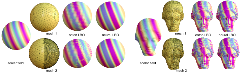
Figure 11. Robustness of Neural LBO. We demonstrate that our optimized eigenfunctions are largely unaffected by differences in mesh density on the starting mesh, because we work directly with a smooth surface. Here we show that while the cotan discretization can be very inconsistent across changes in mesh density, the neural LBO is more consistent when applied to a scalar field defined on an SNS that is generated from different meshes of the same surface.

We evaluate our proposed framework on standard geometry processing tasks. In the context of mesh input, we assess the robustness of our estimates to different meshing of the same underlying surfaces (Figure 11) and isometrically related shapes (Figure 10). We compare the results against ground truth values when they are computable (e.g., analytical functions - see Figure 3 and Figure 4) and contrast them against alternatives, where applicable (Figure 11).

Our main contribution is introducing a novel representation and associated operators to enable neural geometry processing.
We:

1. introduce spherical neural surfaces as a representation to encode genus-0 surfaces seamlessly as overfitted neural networks;

2. compute surface normals, First and Second Fundamental Forms, curvature, continuous Laplace Beltrami operators, and their smallest spectral modes without using any unnecessary discretization;

3. show illustrative applications towards scalar field manipulation and neural mean curvature flow; and

4. demonstrate the robustness and accuracy of the setup on different forms of input.

2. Related Works

Neural representations

Implicit neural representations, such as signed distance functions (SDFs) and occupancy networks, have recently been popularized to model 3D shapes. Notably, DeepSDF (Park et al., 2019) leverages a neural network to represent the SDF of a shape, enabling continuous and differentiable shape representations that can be used for shape completion and reconstruction tasks; (Davies et al., 2020) use neural networks to overfit to individual SDFs; Occupancy Networks (Mescheder et al., 2018) learn a continuous function to represent the occupancy status of points in space, providing a powerful tool for 3D shape modeling and reconstruction from sparse input data. Explicit neural representations, on the other hand, use neural networks to directly predict structured 3D data such as meshes or point clouds. Mesh R-CNN (Gkioxari et al., 2019) extends Mask-RCNN to predict 3D meshes from images by utilizing a voxel-based representation followed by mesh refinement with a graph convolution network operating over the mesh’s vertices and edges. In the context of point clouds, PointNet (Qi et al., 2016) and its variants are widely used as backbones for shape understanding tasks like shape classification and segmentation. Hybrid representations combine the strengths of both implicit and explicit methods. For example, Pixel2Mesh (Wang et al., 2018) generates 3D meshes from images by progressively deforming a template mesh using a graph convolutional network, integrating the detailed geometric structure typical of explicit methods with the continuous nature of implicit representations. More relevant to our work is the AtlasNet (Groueix et al., 2018) that models surfaces as a collection of parametric patches, balancing flexibility and precision in shape representation, and Neural Surface Maps (Morreale et al., 2021), which are overfitted to a flattened disc parametrization of surfaces to enable surface-to-surface mapping.

Estimating differential quantities

Traditionally, researchers have investigated how to carry over differential geometry concepts (do Carmo, 1976) to surface meshes, where differential geometry does not directly apply because mesh faces are flat, with all the ‘curvature’ being at sharp face intersections. Taubin (1995) introduce several signal processing operators on meshes. Meyer et al. (2002) used averaging Voronoi cells and the mixed Finite-Element/Finite-Volume method; (Cazals and Pouget, 2005) used osculating jets; while (de Goes et al., 2020) used discrete differential geometry (Desbrun et al., 2006) to compute gradients, curvatures, and Laplacians on meshes. Recently, researchers have used learning-based approaches to ‘learn’ differential quantities like normals and curvatures on point clouds (Guerrero et al., 2018; Ben-Shabat et al., 2019; Pistilli et al., 2020).

More related to ours is the work by Novello et al. (2022), who represent surfaces via implicit functions and analytically compute differential quantities such as normals and curvatures. With a similar motivation, Chetan et al. (2023) fit local polynomial patches to obtain more accurate derivatives from pre-trained hybrid neural fields; they also use these as higher-order constraints in the neural implicit fitting stage. A similar idea was explored by Bednarik et al. (2020), as a regularizer for the AtlasNet setup, by using implicit differential surface properties during training. The work by Yang and colleagues (2021) is closest to ours in motivation - they also mainly focus on normal and curvature estimates but they additionally demonstrate how to perform feature smoothing and exaggeration using the local differential quantities in the target loss functions and thus driving the modification of the underlying neural fields. However, we go beyond normal and curvature estimates and focus on operators such as surface gradient, surface divergence and Laplace Beltrami operators for processing scalar and vector fields defined on the surfaces.

Laplace Beltrami operators on meshes

The Laplace-Beltrami operator (LBO) is an indispensable tool in spectral geometry processing, as it can be used analyze and manipulate the intrinsic properties of shapes. Spectral mesh processing (Lévy and Zhang, 2010) leverages the eigenvalues and eigenfunctions of the LBO for tasks such as mesh smoothing and shape segmentation. Many subsequent efforts have demonstrated the use of LBO towards shape analysis and understanding (e.g., shapeDNA (Reuter et al., 2006), global point signatures (Rustamov, 2007), heat kernel signature (Sun et al., 2009)), eventually culminating into the functional map framework (Ovsjanikov et al., 2012). An earlier signal processing framework (Taubin, 1995) has been revisited with the LBO operator (Lévy and Zhang, 2010) for multi-scale processing applications (e.g., smoothing and feature enhancement). Although the Laplace-Beltrami operator on triangular meshes or, more generally, on polyhedral meshes, can be computed, these operators depend on the underlying discretization of the surface (i.e., placement of vertices and their connectivity). See (Bunge et al., 2023) for a discussion. In the case of triangular meshes, the commonly used discretizations are the Uniform LBO and the cotan LBO. In Section 6, we compare our neural LBO with the cotan discretization and discuss their relative merits.

3. Spherical Neural Surfaces

We introduce a new neural representation called a ‘Spherical Neural Surface’ (SNS) to represent continuous surfaces. An SNS is a Multi-Layer Perceptron (MLP) $S_{\theta}:\,\mathbb{R}^{3}\rightarrow\mathbb{R}^{3}$, which we train so that the restriction to the unit sphere ($\mathbb{S}^{2}\subset\mathbb{R}^{3}$) is a continuous parametrization of a given surface. In terms of notation, we will also use $S_{\theta}$ or $S$ as shorthand for the set $S_{\theta}(\mathbb{S}^{2})$. In our current work, we primarily focus on creating SNSs from input triangle-meshes and analytically-defined surfaces, but there is potential to create SNSs from other representations such as pointclouds, SDFs, etc. Figure 12 shows initial results for generating an SNS from a neural SDF.

3.1. Overfitting an SNS to a Triangle-Mesh

Given a genus-0 manifold triangle-mesh, we first find an injective embedding of the mesh vertices onto the unit sphere, using a spherical embedding algorithm (Schmidt et al., 2023; Praun and Hoppe, 2003). We extend the embedding to a continuous embedding by projecting points on the sphere to the discrete sphere, and employing barycentric coordinates so that every point $p_{i}$ on the sphere corresponds to a unique point $q_{i}$ on the target surface. We overfit the network $S_{\theta}$ to this parametrization by minimizing the MSE between the ground truth and predicted surface positions, as:

(1) $$\mathcal{L}_{MSE}:=\frac{1}{N}\sum\limits_{i=1}^{N}\left\|S_{\theta}(p_{i})-q_{i}\right\|^{2}.$$

Further, to improve the fitting, we encourage the normals derived from the spherical map to align with the normals of points on the mesh, via a regularization term,

(2) $$\mathcal{L}_{\textit{normal}}:=\frac{1}{N}\sum_{i=1}^{N}\left\|\mathbf{n}_{S_{\theta}}({p_{i}})-\mathbf{n}_{\textit{mesh}}({p_{i}})\right\|^{2}=\frac{2}{N}\sum_{i=1}^{N}(1-\cos{\alpha_{i}(p_{i})}).$$

In this expression, $\mathbf{n}_{\textit{mesh}}({p_{i}})$ is the (outwards) unit-normal on the mesh, and $\mathbf{n}_{S_{\theta}}({p_{i}})$ is the corresponding (outwards) unit-normal of the smooth parametrization at $p_{i}$, which is derived analytically from the Jacobian of $S_{\theta}$ at $p_{i}$ (see Section 3.2); the angle $\alpha(p_{i})$ is the angle between $\mathbf{n}_{\textit{mesh}}({p_{i}})$ and $\mathbf{n}_{S_{\theta}}({p_{i}})$. See Figure 2 for an example.

Figure 2. Spherical Neural Surface. Given an input surface — a mesh in this case — we progressively overfit an MLP to represent the surface as $S_{\theta}$. The loss term is simply the MSE between the ground truth and predicted surface positions, plus a (scaled) normals regularization term (Equation 2).

3.2. Computing Differential Quantities using SNS

One of the advantages of Spherical Neural Surfaces as a geometry representation is that it is extremely natural to compute many important quantities from continuous differential geometry - without any need for approximation or discretization. This is thanks to the automatic differentiation functionality built into modern machine learning setups and algebraically tracking some changes of variables.

For example, to compute the outwards-pointing normal $\mathbf{n}_{S}$, we simply compute the $3\times 3$ Jacobian of $S$ — $\mathbf{J}({S})$ — and then turn this into a Jacobian for a local 2D parametrization by composing it with a $3\times 2$ orthonormal matrix ($R$):

(3) $$\mathbf{J}^{\textit{local}}_{S}=\mathbf{J}({S})\,R=\begin{pmatrix}\textbar&\textbar\\ S_{u}&S_{v}\\ \textbar&\textbar\\ \end{pmatrix}.$$

The columns of $\mathbf{J}^{\textit{local}}_{S}$ are the partial derivatives $S_{u}$ and $S_{v}$. The matrix $R$ defines orthogonal unit vectors on the tangent plane of the sphere at each point, and the functions $u$ and $v$ are the corresponding orthonormal coordinates on the tangent plane of the sphere. Then, the normalized cross product of $S_{u}$ and $S_{v}$ is the outward-pointing unit normal to the surface:

(4) $$\mathbf{n}_{S}=\frac{S_{u}\times S_{v}}{\left\|S_{u}\times S_{v}\right\|}.$$

In terms of standard spherical polar coordinates ($\theta$ and $\phi$), we chose to use the following rotation matrix:

(5) $$R=\begin{pmatrix}\cos\theta\cos\phi&-\sin\phi\\ \cos\theta\sin\phi&\cos\phi\\ -\sin\theta&0\\ \end{pmatrix}.$$

This matrix is an orthonormal version of the usual spherical polar coordinates Jacobian. We avoid degeneracy at the poles by selectively re-labeling the $x$, $y$, and $z$ coordinates so that $\theta$ is never close to zero or $\pi$.

Now, from $\mathbf{J}^{\textit{local}}_{S}$, we can simply write the First Fundamental Form (FFF) of the sphere-to-surface map as:

(6) $$\mathbf{I}_{S}=\begin{pmatrix}E&F\\ F&G\\ \end{pmatrix}=(\mathbf{J}^{\textit{local}}_{S})^{T}\,\mathbf{J}^{\textit{local}}_{S}.$$

To compute the Second Fundamental Form (SFF), we first compute the second partial derivatives of the parametrization with respect to the local co-ordinates, and then find the dot products of the second derivatives with the normal, $\mathbf{n}=\mathbf{n}_{S_{\theta}}$. The second derivatives are:

(7) $$S_{uu}=\mathbf{J}(S_{u})S_{u},\quad S_{uv}=\mathbf{J}(S_{u})S_{v},\quad S_{uu}=\mathbf{J}(S_{v})S_{v}.$$

We can now express the SFF as:

(8) $$\mathbf{II}_{S}=\begin{pmatrix}e&f\\ f&g\\ \end{pmatrix}=\begin{pmatrix}S_{uu}\cdot\mathbf{n}&S_{uv}\cdot\mathbf{n}\\ S_{uv}\cdot\mathbf{n}&S_{vv}\cdot\mathbf{n}\\ \end{pmatrix}.$$

In terms of the FFF and SFF, the Gauss curvature is

(9) $$K=\frac{eg-f^{2}}{EG-F^{2}},$$

and the mean curvature is

(10) $$H=\frac{Eg-2Ff+Ge}{2(EG-F^{2})}.$$

Furthermore, we can algebraically solve the quadratic equation $\text{det}(\mathbf{I}_{S}-\lambda\mathbf{II}_{S})=0$, to obtain explicit expressions for the principal curvatures, that we then use to find the principal curvature directions directly on the Spherical Neural Surface. In Figure 3, we compare our differential estimates against analytical computations for an analytic surface; in Figure 6 we also show curvature estimates and principal curvature directions on other SNS approximations of input triangle meshes (ground truth values are not available).

Figure 3. First and Second Fundamental Forms. Here, we display the differential quantities computed using our framework, on an SNS that has been overfitted to the mesh of a surface with an analytical parametrization (bottom) and we show that the results are extremely close to the differential quantities that have been computed symbolically, using Matlab.

4. Mathematical Background

This section briefly summarizes the relevant background for continuous surfaces that we need to develop a computation framework for Laplace-Beltrami and spectral analysis using SNS (Section 5).

4.1. The Laplace Beltrami Operator on Smooth Surfaces

The (Euclidean) Laplacian $\Delta$ of a scalar field $f:\mathbb{R}^{n}\rightarrow\mathbb{R}$ is defined as the divergence of the gradient of the scalar field. Equivalently, $\Delta f$ is the sum of the unmixed second partial derivatives of the field $f$:

(11) $$\Delta f:=\nabla\cdot\nabla f=\sum_{i=1}^{n}\frac{\partial^{2}f}{\partial^{2}x_{i}}.$$

The Laplace-Beltrami operator, or surface Laplacian, is the natural generalization of the Laplacian to scalar fields defined on curved domains. If $\Sigma\subset\mathbb{R}^{3}$ is a regular surface and $f:\Sigma\rightarrow\mathbb{R}$ is a scalar field, then the Laplace-Beltrami operator on $f$ is defined as the surface divergence of the surface gradient of $f$, and we denote this by $\Delta_{\Sigma}f$ to emphasize the dependence on the surface $\Sigma$. Thus,

(12) $$\Delta_{\Sigma}f:=\nabla_{\Sigma}\cdot\nabla_{\Sigma}f.$$

The surface gradient of the scalar field $f$ (written $\nabla_{\Sigma}f$), and the surface divergence of a vector field ${\mathbf{F}}:\Sigma\rightarrow\mathbb{R}^{3}$ (written $\nabla_{\Sigma}\cdot F$), can be computed by smoothly extending the fields to fields $\tilde{f}$ and $\tilde{\mathbf{F}}$ respectively, which are defined on a neighborhood of $\Sigma$ in $\mathbb{R}^{3}$.

The surface gradient is defined as the projection of the gradient of $\tilde{f}$ into the local tangent plane:

(13) $$\nabla_{\Sigma}f=\nabla\tilde{f}-(\nabla\tilde{f}\cdot\mathbf{n})\mathbf{n},$$

where $\mathbf{n}$ is the unit surface normal at the point. The surface divergence of the vector field $\mathbf{F}$ is defined as

(14) $$\nabla_{\Sigma}\cdot\mathbf{F}=\nabla\cdot\tilde{\mathbf{F}}-\mathbf{n}^{T}{\mathbf{J}}(\tilde{\mathbf{F}})\mathbf{n},$$

where $\mathbf{J}(\tilde{\mathbf{F}}):=\begin{bmatrix}\frac{\partial{\tilde{\mathbf{F}}}}{\partial{x_{1}}},&\frac{\partial{\tilde{\mathbf{F}}}}{\partial{x_{2}}},&\frac{\partial{\tilde{\mathbf{F}}}}{\partial{x_{3}}}\\ \end{bmatrix}$ is the Jacobian of $\mathbf{F}$. Since $\mathbf{J}(\tilde{\mathbf{F}})\mathbf{n}$ is the directional derivative of $\tilde{\mathbf{F}}$ in the normal direction, then $\mathbf{n}^{T}\mathbf{J}(\tilde{\mathbf{F}})\mathbf{n}=\mathbf{J}(\tilde{\mathbf{F}})\mathbf{n}\cdot\mathbf{n}$ can be thought of as the contribution to the three-dimensional divergence of $\tilde{\mathbf{F}}$ that comes from the normal component of $\tilde{\mathbf{F}}$, and by ignoring the contribution from the normal component, we get the two-dimensional ‘surface divergence’. Although these expressions depend a-priori on the particular choice of extension, the surface gradient and surface divergence are in fact well-defined (i.e., any choice of extension will give the same result).

By expanding out the definitions of surface gradient and surface divergence, we can derive an alternative formula for the surface Laplacian ($\Delta_{\Sigma}f$) in terms of the (Euclidean) Laplacian ($\Delta\tilde{f}$), the gradient ($\nabla\tilde{f}$) and the Hessian ($\mathbf{H}(\tilde{f})=\mathbf{J}(\nabla\tilde{f})^{T}$) as,

(15) $$\Delta_{\Sigma}f=\Delta\tilde{f}-2H\nabla\tilde{f}\cdot\mathbf{n}-\mathbf{n}^{T}\mathbf{H}(\tilde{f})\mathbf{n}.$$

The dependence on the surface is captured by the normal function $\mathbf{n}$, and the mean curvature $H$. Please refer to (Reilly, 1982; Xu and Zhao, 2023) for a derivation. In the case when $\tilde{f}$ is a ‘normal extension’ — i.e., it is locally constant in the normal directions close to the surface — then the second and third terms disappear, meaning that $\Delta_{\Sigma}f$ is consistent with $\Delta\tilde{f}$.

If we substitute in the coordinate function $\mathbf{x}$, then the first and third terms disappear in the above equation, and we are left with the familiar equation,

(16) $$\Delta_{\Sigma}\mathbf{x}=-2H\mathbf{n}.$$

This formula is often used in the discrete setting to compute the mean curvature from the surface Laplacian.

4.2. Spectrum of the Laplace Beltrami Operator

Given two scalar functions, $f$ and $g$, defined on the same regular surface $\Sigma$, we can define their inner product to be,

(17) $$\left<f,g\right>_{L^{2}(\Sigma)}:=\int_{\Sigma}fg\,dA\,.$$

Then, the $L^{2}$ norm of a scalar function can be expressed as,

(18) $$\left\|f\right\|_{L^{2}(\Sigma)}=\sqrt{\left<f,f\right>_{L^{2}(\Sigma)}}=\sqrt{\int_{\Sigma}|f|^{2}\,dA}\,.$$

The Laplace Beltrami operator, $\Delta_{\Sigma}$, is a self-adjoint linear operator with respect to this inner product. This means that there is a set of eigenfunctions of $\Delta_{\Sigma}$ that form an orthonormal basis for the space $L^{2}(\Sigma)$ - the space of ‘well-behaved’ scalar functions on $\Sigma$ that have a finite $L^{2}$-norm. This basis is analogous to the Fourier basis for the space of periodic functions on an interval.

In the discrete mesh case, the eigenfunctions of the Laplace-Beltrami operator are computed by diagonalizing a sparse matrix (Lévy and Zhang, 2010; Bunge et al., 2023) based on the input mesh. In the continuous case, however, we no longer have a matrix representation for $\Delta_{\Sigma}$. Instead, we exploit a functional analysis result that describes the first $k$ eigenfunctions of $\Delta_{\Sigma}$ as the solution to a minimization problem, as described next.

First, we define the Rayleigh Quotient of a scalar function $f$ to be the Dirichlet energy of the scalar function, divided by the squared $L^{2}$-norm of the function:

(19) $$Q_{\Sigma}(f):=\frac{\left\|\nabla_{\Sigma}f\right\|_{L^{2}(\Sigma)}^{2}}{\left\|f\right\|^{2}_{L^{2}(\Sigma)}}.$$

Then, the eigenfunctions of $\Delta_{\Sigma}$ are the minimizers of the Rayleigh Quotient, as given by,

$$\Psi_{0},\Psi_{1},...,\Psi_{k-1}=\text{argmin}_{\Psi_{0}^{*},...,\Psi_{k-1}^{*}}\sum_{i=0}^{k-1}Q_{\Sigma}(\Psi_{i}^{*})$$

(20) $$\textit{such that}\quad\left<\Psi_{i},\Psi_{j}\right>_{L^{2}(\Sigma)}=0\quad\text{for all}\quad i\neq j.$$

We use $\Psi_{0}$ to represent the first eigenfunction, which is always a constant function. The constraint states that the eigenfunctions are orthogonal inside the inner-product space $L^{2}(\Sigma)$.

Figure 4. Neural Spectral Basis against Analytical Solutions. The sphere is a genus-0 surface for which the eigenspaces of the Laplace-Beltrami operator are very well understood: the eigenspaces are the spaces spanned by linear combinations of the spherical harmonics for each frequency. This means that each of our optimized eigenfunctions should belong to one of these eigenspaces, and therefore, the Rayleigh quotient should match the energy level of the corresponding spherical harmonics. For evaluation, we compute the Rayleigh quotient using a large number of samples for Monte Carlo integration, since we cannot analytically compute the integral. For reference, we present the ground truth Rayleigh quotients, in green.

In addition, the Rayleigh Quotient of the eigenfunction $\Psi_{i}$ is the positive of the corresponding eigenvalue, i.e.,

(21) $$\Delta_{\Sigma}\Psi_{i}(x)=-Q_{\Sigma}(\Psi_{i})\Psi_{i}(x)\quad\forall\,x\in\Sigma.$$

Physically, the eigenfunctions of $\Delta_{\Sigma}$ represent the fundamental modes of vibration of the surface $\Sigma$. The Rayleigh Quotient of $\Psi_{0}$ is zero, and as the Rayleigh quotient increases, the vibrational modes increase in energy and the eigenfunctions produce more ‘intricate’ (high frequency) patterns.

Figure 5. Encoding Scalar Fields on Neural Surfaces. We encode scalar fields on the sphere (and corresponding extensions into $\mathbb{R}^{3}$) as MLPs
$g_{\eta}:\mathbb{R}^{3}\rightarrow\mathbb{R}$. Because $S_{\theta}$, considered as a parametrization, is bijective, then we can implicitly define any smooth scalar field $h$ on the surface in terms of one of the functions $g_{\eta}$ (restricted to $\mathbb{S}^{2}$). We visualize the one-to-one correspondence between scalar fields defined on the surface, and scalar fields defined on the sphere, by using vertex-colors to display the fields.

Figure 6. First and Second Fundamental Forms. An SNS represents a smooth, seamless parametrization of a genus-0 surface, and we can compute the partial derivatives of this parametrization using automatic differentiation. We compute the normals and the First Fundamental Form of the parametrization from the first derivatives. Subsequently, computing the second derivatives enables us to construct the Second Fundamental Form of the parametrization. Hence, we compute Mean Curvature, Gaussian Curvature, and Principal Curvature Directions at any point without any unnecessary discretization error.

5. Spectral Analysis using SNS

To find the continuous eigenmodes of the Laplace-Beltrami operator on an SNS, we require a continuous and differentiable representation for scalar functions defined on the surface. In our framework, we represent such smooth scalar fields on $\mathbb{S}^{2}$ by MLPs, $g_{\eta}$, from $\mathbb{R}^{3}$ to $\mathbb{R}$. We only ever evaluate the MLP $g_{\eta}$ on $\mathbb{S}^{2}\in\mathbb{R}^{3}$, but because the domain is $\mathbb{R}^{3}$ then it defines an extension of the scalar field, and this allows us to compute $\nabla g_{\eta}$. Then, if $S_{\theta}:\mathbb{R}^{3}\rightarrow\mathbb{R}^{3}$ is an SNS, any smooth scalar field $h$ defined on $S_{\theta}$ can be defined implicitly by the equation,

(22) $$h\circ S_{\theta}=g_{\eta}.$$

Applying the chain rule to the implicit equation, we can compute the gradient of $h$:

(23) $$\nabla h=(\mathbf{J}(S_{\theta})^{T})^{-1}\nabla g_{\eta},$$

which allows us to compute $\nabla_{S_{\theta}}h$ (Equation 13) and $Q_{S_{\theta}}(h)$ (Equation 19) without explicitly computing $h$.

To optimize for a (smooth) scalar function $g_{\eta_{k}}$ so that $h$ approximates the $k$th non-constant eigenfunction of the Laplace-Beltrami operator, we use gradient descent to optimize the weights, $\eta_{k}$. We use a combination of two loss terms:

(24) $$\mathcal{L}_{Rayleigh}:=Q_{S}(h)\quad\text{and}\quad\mathcal{L}_{ortho}:=\sum_{i=0}^{k-1}\left<h,h_{i}\right>_{L^{2}(S)}^{2},$$

where we sequentially compute the eigenfunctions, and $h_{i}$ is the $i$th smallest eigenfunction to be found. Recall that we represent each such eigenfunction using a dedicated MLP (except for $h_{0}$, which is the constant eigenfunction). The loss term $\mathcal{L}_{ortho}$ encourages the scalar field $h$ to be orthogonal to all previously-found eigenfunctions (including the constant eigenfunction). The quantity $Q_{S_{\theta}}(h)$ depends on the Jacobian of $S_{\theta}$, through $\nabla_{S_{\theta}}h$ and $\nabla h$. However, since the surface does not change during optimization and $\theta$ stays fixed, we precompute $(\mathbf{J}(S_{\theta})^{T})^{-1}$. Note that, if we were to optimize over the subspace of the unit-norm functions in $L^{2}(\Sigma)$, then we could replace the Rayleigh Quotient with the Dirichlet energy. However, it was a more natural design choice for us to parametrize the entire space $L^{2}(\Sigma)$ and optimize the Rayleigh Quotient, rather than to parametrize only the space of unit-norm functions in $L^{2}(\Sigma)$ and minimize the Dirichlet Energy.

Additionally, for stability, we included a regularization term designed to keep the $L^{2}$-norm of $h$ close to one:

(25) $$\mathcal{L}_{unit}:=(\left\|h\right\|_{L^{2}(S)}-1)^{2}.$$

The combined loss term is expressed as,

(26) $$\mathcal{L}=\mathcal{L}_{Rayleigh}+\lambda_{ortho}\mathcal{L}_{ortho}+\lambda_{unit}\mathcal{L}_{unit}.$$

We choose large initial values for the coefficients because we find that this improves stability, and then we reduce the coefficients so that the Rayleigh Quotient is the dominant term during the later stages of optimization (see Section 6 for details).

Finally, since we cannot exactly compute the inner products in these loss terms, we approximate the inner products by Monte-Carlo sampling. Specifically, we approximate,

(27) $$\left<f,g\right>_{L^{2}(S)}\approx\frac{Area(S)}{N}\sum_{i=1}^{N}f(p_{i})g(p_{i}),$$

where $\{p_{i}\}_{1\leq i\leq N}$ is a set of uniformly distributed points on the surface $S_{\theta}$; $f(p_{i})$ and $g(p_{i})$ denote calls to the scalar field MLPs. (In the overfitting stage, we normalize all our Spherical Neural Surfaces to have an area equal to $4\pi$.) For the Monte Carlo step, we generate $N$ uniformly distributed points on the surface $S_{\theta}$ via the following steps (rejection sampling):

1. Generate $M\gg N_{target}$ samples ($p_{i}$) from the 3D normal distribution $\mathcal{N}(\mathbf{\mu}=\mathbf{0},\mathbf{\Sigma}=\mathbf{I})$. Normalize, to unit norm, to produce a dense uniform distribution of points on the sphere $\mathbb{S}^{2}\subset\mathbb{R}^{3}$.

2. Compute the local area distortion ($d_{i}=\sqrt{E_{i}G_{i}-F_{i}^{2}}$), for each point $p_{i}$, using the First Fundamental Form.

3. Perform rejection sampling, such that the probability of keeping point $p_{j}$ is equal to $\frac{d_{j}}{\sum_{i=1}^{M}d_{i}}N_{target}$.

Following this process, the expected number of points will equal $N_{target}$ — a specified parameter — however, the actual number of points ($N$) may vary.

Figure 7. Spectral Modes on Neural Surfaces. We propose how to compute the lowest few spectral modes of the neural Laplace Beltrami operator $\Delta_{S_{\theta}}$ via minimization of the Rayleigh quotient, without requiring any unnecessary discretization. Here we show the lowest few spectral modes of different SNSs. The lowest spectral mode is constant, and not included in this figure. Each of the spectral modes is represented by a dedicated MLP (see Equation 22).

Figure 8. Heat Flow (left) and Mean Curvature Flow (right). (Left) We can evolve a given scalar field, $f$, specified over the surface of an SNS, $S_{\theta}$, using the Partial Differential Equation (PDE) $f_{t}=\Delta_{S_{\theta}}f$ (the heat equation). We represent the evolving scalar field as a small MLP, whose weights are ‘finetuned’ for up to 100 epochs after every time step. Darker colors denote low values (cold) with lighter colors being high (hot). (Right) Taking advantage of the differentiable nature of our representation, we can also compute a mesh-free Mean Curvature Flow (MCF) in which the Mean Curvature and normals are updated at every iteration. We update the Spherical Neural Surface using a small number of finetuning steps, after every iteration of the flow. This formulation of MCF prevents singularities from forming, without any special handling to prevent them (Kazhdan et al., 2012).

Figure 9. Laplace Beltrami on Neural Scalar Fields. We present two ways to compute Laplace Beltrami operators on any smooth scalar field, $f$, defined on a neural surface $S_{\theta}$ (top): first, using mean curvature estimates (top-middle) (Equation 15) and second, using the divergence of gradient definition (divgrad) (bottom-middle) (Equation 12). We represent scalar fields on surfaces using dedicated MLPs. (Bottom) For comparison, we also show results using the cotan LBO (with a lumped mass matrix) on a dense mesh, whose vertices are the image of the vertices in a dense icosphere mesh under the transformation $S_{\theta}$.

Figure 10. Spectral SNS Modes across Isometric Poses. If we compute the first few eigenfunctions on SNSs that represent near-isometric surfaces, and order the functions according to their Rayleigh quotients, we see a clear correspondence between corresponding eigenfunctions on each surface. Although our computation of the LBO and its spectrum involves extrinsic terms such as mean curvature and normals, the Laplace Beltrami operator is intrinsic so its spectrum does not depend on the particular embedding of a surface into $\mathbb{R}^{3}$, therefore the eigenmodes of isometric SNSs should appear similar (up to a possible sign change).

6. Evaluation

Implementation Details

All of our networks in our experiments were trained on Nvidia GeForce P8 GPUs. The SNS network is a Residual MLP with input and output of size three, and eight hidden layers with 256 nodes each. The networks used to represent scalar fields (in the eigenfunction and heat flow experiments) are very small Residual MLPs with input size three, output size three and two hidden layers with 10 nodes each. (To make the output value a scalar, we take the mean of the three output values.) For both scalar fields and SNS, the activation function is ‘Softplus’. We use the RMSProp optimizer with a learning rate of $10^{-4}$ and a momentum of 0.9. We trained each SNS for up to 20,000 epochs (eight-to-ten hours), and we fixed the normals regularization coefficient to be $10^{-4}$. The time per epoch increases slightly with the number of vertices in the mesh, but for simpler shapes (such as the sphere) the optimization converges in fewer epochs.

Eigenfunction Optimization

In the eigenfunction experiment, we used the initial parameter values $\lambda_{ortho}=10^{3}$ and $\lambda_{unit}=10^{4}$ and then we reduced the coefficients linearly to $\lambda_{ortho}=1$ and $\lambda_{unit}=10^{2}$, over 10,000 epochs. These settings prevent the scalar field from collapsing to the zero-function during the initial stages of optimization, whilst allowing the Rayleigh Quotient to dominate the loss in the later stages. We optimized each eigenfunction for up to 40,000 epochs (approximately six hours on our setup).

We generate $M=100,000$ points for the initial uniform distribution on the sphere, and we use $N_{target}=10,000$ in the rejection sampling process. The points stay fixed during each optimization stage. We believe that this is a possible reason why the Rayleigh Quotient computed on the training points is often slightly lower than the Rayleigh Quotient that is computed with a different, larger set of uniform samples, and a better sampling strategy might improve the accuracy of our optimization.

Comparison against Analytic Functions

For some of our SNS computations, there exist special cases for which an exact analytic solution can be calculated. To test our estimates of curvature and principal curvature directions, we overfitted an SNS to a mesh of the closed surface with the parametrization

(28) $$\mathbf{r}(\theta,\phi)=(1+0.4\sin^{2}\theta\sin(6\theta)\sin(6\phi))\begin{pmatrix}\sin\theta\cos\phi;\sin\theta\sin\phi;\cos\theta\end{pmatrix}.$$

We used the Matlab Symbolic Math Toolbox™ to compute the normals, mean curvature, Gauss curvature and principal curvature directions in closed form. In Figure 3, we show these differential quantities on the mesh of the analytic surface and on the SNS. The computed curvatures align extremely closely, therefore the overfitting quality is very high and the curvature computations are accurate. There is a slight discrepancy at the poles, because we have used a global analytic parametrization which not valid where $\theta\in\{0,\pi\}$. On the other hand, in the SNS formulation we use selective co-ordinate relabelling to avoid issues related to using spherical polar co-ordinates close to the poles.

For evaluation of our optimized eigenfunctions, we overfitted an SNS to a sphere-mesh with 10,242 vertices and optimized for the first five non-constant eigenfunctions. The eigenspaces of the LBO on a sphere are the spaces spanned by the spherical harmonics of each frequency (refer to (Jarosz, 2008)). The first three spherical harmonics have eigenvalue -2 and the following five spherical harmonics have eigenvalue -6. Although the basis for each eigenspace is not unique, the first three eigenfunctions should also have an eigenvalue of -2 and the following five eigenfunctions should have an eigenvalue of -6, meaning that the Rayleigh Quotients should be equal to 2 and 6 (see Figure 4). We computed the ground-truth eigenvalues by manually integrating the Cartesian formulas (Jarosz, 2008) and we estimated the integral of the neural eigenfunctions using 100k Monte Carlo samples. Estimates were within $1\%$ of the ground-truth, and four out of five results were within $0.5\%$.

Neural LBO on Scalar Fields

To evaluate the accuracy of our Laplace-Beltrami operator on SNSs, we generated random scalar fields using sine waves, and visually compared the results of applying three different forms of the LBO, on five different surfaces (see Figure 9). To compute $\Delta_{S_{\theta}}f$ using the mean curvature formulation (Equation 15), we computed the gradient and Hessians of the scalar field analytically and combined these with the SNS estimates of the normals and mean curvature. We also computed $\Delta_{S_{\theta}}f$ using the ‘divergence of gradient’ definition (Equation 12) - in this version, all of the differential calculations were carried out by autograd. We show the results using vertex-colors, on a dense icosphere mesh.

Finally, we computed the result of applying the cotan LBO to the scalar field (sampled at the vertices of the dense icosphere mesh). At this resolution, all three versions of the LBO are extremely close, however, we notice that the cotan estimate on the ‘spike ball’ (column 2) contains a small discontinuity, not present in the SNS estimates. From a smooth shape and a smooth scalar field, the resulting $\Delta_{S}$ should be smooth, which is the case for SNS estimates.

Heat Flow and Mean Curvature Flow

We can approximate the evolution of any initial scalar field $f$ on an SNS $S_{\theta}$, according to the process defined by the heat equation, $f_{t}=\Delta_{S_{\theta}}f.$ In our implementation, we represent the field $f$ implicitly, using Equation 22. In each time step, we compute $\Delta_{S_{\theta}}f$ for the current scalar field $f$, using the divergence of gradient formula in Equation 12. Then we select a small value ($d=10^{-3}$) and we compute $f+d\Delta_{S_{\theta}}f$ at some fixed sample points (in Figure 8-left, we used 10,242 points). We then update the scalar field, by finetuning the network for up to 100 epochs to fit the new sample points, using a simple MSE loss. Qualitatively, the experiment aligns with our expectations. The scalar field gradually becomes more smooth over time, and cold areas warm up to a similar heat level as the surroundings.

Similarly, we approximate a Mean Curvature Flow of an SNS by updating the SNS to $S_{\theta}-dH\mathbf{n}$ at each time step, and finetuning for up to 100 epochs. The results in Figure 8-right show the spiky analytic shape becoming closer to a sphere, over 150 iterations.

Figure 12. Handling Neural Implicits. Spherical Neural Surfaces can be generated from other neural representations, such as DeepSDF. Here, we have produced an SNS from a DeepSDF representation for a camera, by overfitting the SNS to a low-resolution marching-cubes mesh reconstruction and then finetuning this SNS to better align with the SDF.

Neural Implicits

To demonstrate robustness to the input representation, we provide an illustratory example of an SNS generated from a DeepSDF (Park et al., 2019), and show the normals and principal curvature directions on its SNS. We took a pretrained DeepSDF network and the optimized latent code for the camera shape (Comi, 2023). Then, as initialization, we overfitted an SNS to a coarse marching-cubes mesh. Then we took a set of samples on the SNS and projected them to deepSDF representation defined by the signed distance function (SDF), by moving them in the direction of the gradient of the SDF (which approximates the surface normal) by the signed distance at that point, and use them to finetune the SNS.

7. Conclusion

We have presented spherical neural surfaces as a novel representation for genus-0 surfaces along with supporting operators in the form of differential geometry estimates (e.g., normals, First and Second Fundamental Forms), as well as surface gradients and surface divergence operators. We also presented how to compute a continuous Laplace Beltrami operator and its lowest spectral modes. We demonstrated that ours, by avoiding any unnecessary discretization, produces robust and consistent estimates even under different meshing concerning vertex sampling as well as their connectivity.

Limitations and Future Work

Beyond genus-0 surfaces

Since our SNSs rely on a sphere for the parametrization, it limits us to genus-0 surfaces. If we could choose from a range of canonical surfaces (e.g., torus), this would allow us to seamlessly process higher genus shapes and, possibly, to produce neural surfaces without such high distortions. Another option would be to rely on local parametrizations, but then we would have to consider blending across overlapping parametrizations.

Speed

A severe limitation of our current realization is its long running time. While we expect that better and optimized implementations would increase efficiency significantly, we also need to make changes to our formulation. Specifically, our current spectral estimation is sequential, which is not only slow, but leads to an accumulation of errors for later spectral modes. Hence, in the future, we would like to jointly optimize for multiple spectral modes.

SNS from neural representations

We demonstrated our setup mainly on mesh input and also on neural input in the form of deepSDF. In the future, we would like to extend our SNS to other neural representations in the form of occupancy fields or radiance fields. However, this will require locating and sampling points on the surfaces, which are implicitly encoded – we need the representation to provide a projection operator. We would also like to support neural surfaces that come with level-of-detail. Finally, an interesting direction would be to explore end-to-end formulation for dynamic surfaces encoding temporal surfaces with SNS, and enabling optimization with loss terms involving first/second fundamental forms as well as Laplace-Beltrami operators (e.g., neural deformation energy).

Acknowledgements

This project has received funding from the UCL AI Centre. RW wishes to thank Johannes Wallner for his constructive comments regarding Section 4.

References

- (1)
- Bednarik et al. (2020) Jan Bednarik, Shaifali Parashar, Erhan Gundogdu, Mathieu Salzmann, and Pascal Fua. 2020. Shape Reconstruction by Learning Differentiable Surface Representations. In Proceedings IEEE Conf. on Computer Vision and Pattern Recognition (CVPR).
- Ben-Shabat et al. (2019) Yizhak Ben-Shabat, Michael Lindenbaum, and Anath Fischer. 2019. Nesti-Net: Normal estimation for unstructured 3D point clouds using convolutional neural networks. In Proceedings of the IEEE/CVF Conference on Computer Vision and Pattern Recognition (CVPR). IEEE, 10112–10120.
- Bunge et al. (2023) Astrid Bunge, Marc Alexa, and Mario Botsch. 2023. Discrete Laplacians for General Polygonal and Polyhedral Meshes. In SIGGRAPH Asia 2023 Courses. Association for Computing Machinery, Article 7, 49 pages.
- Cazals and Pouget (2005) Frédéric Cazals and Mireille Pouget. 2005. Estimating differential quantities using polynomial fitting of osculating jets. Computer Aided Geometric Design 22, 2 (2005), 121–146. https://doi.org/10.1016/j.cagd.2004.06.003
- Chetan et al. (2023) Aditya Chetan, Guandao Yang, Zichen Wang, Steve Marschner, and Bharath Hariharan. 2023. Accurate Differential Operators for Hybrid Neural Fields. arXiv:2312.05984 [cs.CV]
- Comi (2023) Mauro Comi. 2023. DeepSDF-minimal. https://github.com/maurock/DeepSDF/.
- Davies et al. (2020) Thomas Davies, Derek Nowrouzezahrai, and Alec Jacobson. 2020. Overfit Neural Networks as a Compact Shape Representation. CoRR abs/2009.09808 (2020). arXiv:2009.09808 https://arxiv.org/abs/2009.09808
- de Goes et al. (2020) Fernando de Goes, Andrew Butts, and Mathieu Desbrun. 2020. Discrete differential operators on polygonal meshes. ACM Transactions on Graphics (TOG) 39 (2020), 110:1 – 110:14. https://api.semanticscholar.org/CorpusID:221105828
- Desbrun et al. (2006) Mathieu Desbrun, Konrad Polthier, Peter Schröder, and Ari Stern. 2006. Discrete differential geometry - an applied introduction. In ACM SIGGRAPH course notes.
- do Carmo (1976) Manfredo P. do Carmo. 1976. Differential Geometry of Curves and Surfaces. Prentice-Hall.
- Gkioxari et al. (2019) Georgia Gkioxari, Jitendra Malik, and Justin Johnson. 2019. Mesh R-CNN. CoRR abs/1906.02739 (2019). arXiv:1906.02739 http://arxiv.org/abs/1906.02739
- Groueix et al. (2018) Thibault Groueix, Matthew Fisher, Vladimir G. Kim, Bryan Russell, and Mathieu Aubry. 2018. AtlasNet: A Papier-Mâché Approach to Learning 3D Surface Generation. In Proc. CVPR.
- Guerrero et al. (2018) Paul Guerrero, Yanir Kleiman, Maks Ovsjanikov, and Niloy J. Mitra. 2018. PCPNet: Learning Local Shape Properties from Raw Point Clouds. Computer Graphics Forum 37, 2 (2018), 75–85. https://doi.org/10.1111/cgf.13343
- Jarosz (2008) Wojciech Jarosz. 2008. Efficient Monte Carlo Methods for Light Transport in Scattering Media. Ph. D. Dissertation. UC San Diego.
- Kazhdan et al. (2012) Michael Kazhdan, Jake Solomon, and Mirela Ben-Chen. 2012. Can Mean-Curvature Flow Be Made Non-Singular? arXiv:1203.6819 [math.DG]
- Lévy and Zhang (2010) Bruno Lévy and Hao (Richard) Zhang. 2010. Spectral mesh processing. In ACM SIGGRAPH 2010 Courses (Los Angeles, California) (SIGGRAPH ’10). Article 8, 312 pages.
- Mescheder et al. (2018) Lars M. Mescheder, Michael Oechsle, Michael Niemeyer, Sebastian Nowozin, and Andreas Geiger. 2018. Occupancy Networks: Learning 3D Reconstruction in Function Space. CoRR abs/1812.03828 (2018).
- Meyer et al. (2002) Mark Meyer, Mathieu Desbrun, Peter Schröder, and Alan H. Barr. 2002. Discrete Differential-Geometry Operators for Triangulated 2-Manifolds. In International Workshop on Visualization and Mathematics. https://api.semanticscholar.org/CorpusID:11850545
- Mildenhall et al. (2021) Ben Mildenhall, Pratul P. Srinivasan, Matthew Tancik, Jonathan T. Barron, Ravi Ramamoorthi, and Ren Ng. 2021. NeRF: representing scenes as neural radiance fields for view synthesis. Commun. ACM 65, 1 (Dec 2021), 99–106.
- Morreale et al. (2021) Luca Morreale, Noam Aigerman, Vladimir G Kim, and Niloy J Mitra. 2021. Neural Surface Maps. In Proceedings of the IEEE/CVF Conference on Computer Vision and Pattern Recognition. 4639–4648.
- Novello et al. (2022) Tiago Novello, Guilherme Schardong, Luiz Schirmer, Vinícius da Silva, Hélio Lopes, and Luiz Velho. 2022. Exploring differential geometry in neural implicits. Computers and Graphics 108 (2022), 49–60.
- Nsampi et al. (2023) Ntumba Elie Nsampi, Adarsh Djeacoumar, Hans-Peter Seidel, Tobias Ritschel, and Thomas Leimkühler. 2023. Neural Field Convolutions by Repeated Differentiation. ACM Trans. Graph. 42, 6, Article 206 (Dec 2023), 11 pages. https://doi.org/10.1145/3618340
- Ovsjanikov et al. (2012) Maks Ovsjanikov, Mirela Ben-Chen, Justin Solomon, Adrian Butscher, and Leonidas Guibas. 2012. Functional maps: a flexible representation of maps between shapes. ACM Transactions on Graphics (ToG) 31, 4 (2012), 1–11.
- Park et al. (2019) Jeong Joon Park, Peter R. Florence, Julian Straub, Richard A. Newcombe, and Steven Lovegrove. 2019. DeepSDF: Learning Continuous Signed Distance Functions for Shape Representation. CoRR abs/1901.05103 (2019).
- Pistilli et al. (2020) Federico Pistilli, Giulia Fracastoro, Diego Valsesia, and Enrico Magli. 2020. Point Cloud Normal Estimation with Graph-Convolutional Neural Networks. In 2020 IEEE International Conference on Multimedia & Expo Workshops (ICMEW). IEEE, 1–6.
- Praun and Hoppe (2003) Emil Praun and Hugues Hoppe. 2003. Spherical parametrization and remeshing. ACM Trans. Graph. 22, 3 (jul 2003), 340–349.
- Qi et al. (2016) Charles R Qi, Hao Su, Kaichun Mo, and Leonidas J Guibas. 2016. PointNet: Deep Learning on Point Sets for 3D Classification and Segmentation. arXiv preprint arXiv:1612.00593 (2016).
- Reilly (1982) Robert C. Reilly. 1982. Mean Curvature, The Laplacian, and Soap Bubbles. The American Mathematical Monthly 89 (1982), 180–98.
- Reuter et al. (2006) Martin Reuter, Franz-Erich Wolter, and Niklas Peinecke. 2006. Laplace–Beltrami spectra as ‘Shape-DNA’ of surfaces and solids. Computer-Aided Design 38, 4 (2006), 342–366. Symposium on Solid and Physical Modeling 2005.
- Rustamov (2007) Raif Rustamov. 2007. Laplace-Beltrami eigenfunctions for deformation invariant shape representation. In Proceedings of the Symposium on Geometry Processing. Eurographics Association, 225–233.
- Sawhney and Crane (2020) Rohan Sawhney and Keenan Crane. 2020. Monte Carlo geometry processing: a grid-free approach to PDE-based methods on volumetric domains. ACM Trans. Graph. 39, 4, Article 123 (aug 2020), 18 pages.
- Schmidt et al. (2023) Patrick Schmidt, Dörte Pieper, and Leif Kobbelt. 2023. Surface Maps via Adaptive Triangulations. Computer Graphics Forum 42, 2 (2023).
- Sun et al. (2009) Jian Sun, Maks Ovsjanikov, and Leonidas Guibas. 2009. A concise and provably informative multi-scale signature based on heat diffusion. Computer Graphics Forum 28, 5 (2009), 1383–1392.
- Taubin (1995) Gabriel Taubin. 1995. A signal processing approach to fair surface design. In Proceedings of the 22nd Annual Conference on Computer Graphics and Interactive Techniques (SIGGRAPH ’95). Association for Computing Machinery, New York, NY, USA, 351–358. https://doi.org/10.1145/218380.218473
- Wang et al. (2018) Nanyang Wang, Yinda Zhang, Zhuwen Li, Yanwei Fu, Wei Liu, and Yu-Gang Jiang. 2018. Pixel2Mesh: Generating 3D Mesh Models from Single RGB Images. CoRR abs/1804.01654 (2018). http://arxiv.org/abs/1804.01654
- Wardetzky et al. (2007) Max Wardetzky, Saurabh Mathur, Felix Kälberer, and Eitan Grinspun. 2007. Discrete Laplace operators: No free lunch. Proc. SGP 07, 33–37.
- Xu and Zhao (2023) JJ. Xu and HK. Zhao. 2023. An Eulerian Formulation for Solving Partial Differential Equations Along a Moving Interface. Journal of Scientific Computing 19 (2023), 573–594.
- Yang et al. (2021) Guandao Yang, Serge Belongie, Bharath Hariharan, and Vladlen Koltun. 2021. Geometry Processing with Neural Fields. In Thirty-Fifth Conference on Neural Information Processing Systems.