Random unitaries in extremely low depth

Abstract

We prove that random quantum circuits on any geometry, including a 1D line, can form approximate unitary designs over $n$ qubits in $\log n$ depth. In a similar manner, we construct pseudorandom unitaries (PRUs) in 1D circuits in $\text{poly}\log n$ depth, and in all-to-all-connected circuits in $\text{poly}\log\log n$ depth. In all three cases, the $n$ dependence is optimal and improves exponentially over known results. These shallow quantum circuits have low complexity and create only short-range entanglement, yet are indistinguishable from unitaries with exponential complexity. Our construction glues local random unitaries on $\log n$-sized or $\text{poly}\log n$-sized patches of qubits to form a global random unitary on all $n$ qubits. In the case of designs, the local unitaries are drawn from existing constructions of approximate unitary $k$-designs, and hence also inherit an optimal scaling in $k$. In the case of PRUs, the local unitaries are drawn from existing unitary ensembles conjectured to form PRUs. Applications of our results include proving that classical shadows with 1D log-depth Clifford circuits are as powerful as those with deep circuits, demonstrating superpolynomial quantum advantage in learning low-complexity physical systems, and establishing quantum hardness for recognizing phases of matter with topological order.

1 Introduction

Random processes are central to computing technologies [1, 2, 3, 4, 5, 6, 7] and our understanding of the natural world [8, 9, 10, 11, 12, 13, 14]. In quantum systems, the analog of a random process is a Haar-random unitary operation. Random unitaries form the backbone of numerous components of quantum technologies, including quantum device benchmarking [15, 16, 17], efficient observable estimation [18, 19, 20, 21], quantum supremacy demonstrations [22, 23, 24, 25], and quantum cryptography [26, 27, 28]. They also serve as indispensable toy models for complex processes in quantum many-body physics, underlying recent breakthroughs in quantum chaos [29, 30, 31, 32, 33, 34], quantum machine learning [35, 36, 37], and quantum gravity [38, 39, 40, 41, 42, 43].

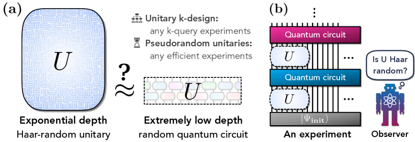
Figure 1: (a) The central question we seek to answer is: How shallow can a random quantum circuit be while replicating the behavior of a Haar-random unitary? A Haar-random unitary over $n$ qubits requires a circuit depth that grows exponentially in $n$. Approximate unitary $k$-designs replicate the behavior of Haar-random unitaries within any quantum experiment that queries the unitary $k$ times. Pseudorandom unitaries replicate the behavior of Haar-random unitaries within any efficient quantum experiment. (b) Any quantum experiment can be represented as follows: an observer prepares an initial state $\ket{\Psi_{\mathrm{init}}}$, applies the unitary $U$ many times, interleaved with many quantum circuits for quantum information processing, and concludes by performing a measurement (not shown).

In all of these applications, a crucial consideration is in what circuit depth a random unitary can be generated. Since a Haar-random unitary requires a depth exponential in the number of qubits, any efficient construction of random unitaries requires a notion of approximation. To this end, approximate unitary designs [44, 45, 46] and pseudorandom unitaries [47] are defined to approximate the action of a Haar-random unitary within any quantum experiment that makes at most $k$ queries to the unitary $U$ (for unitary $k$-designs), or any efficient quantum experiment (for pseudorandom unitaries); see Fig. 1. Enormous effort has gone into constructing approximate unitary designs and pseudorandom unitaries in as low a depth as possible [48, 49, 50, 51, 52, 53, 54, 55, 56, 57, 58, 59, 60, 61, 62, 47, 63, 64, 65]. To date, for both unitary designs and pseudorandom unitaries, all known constructions require a depth polynomial in the number of qubits $n$.

In this work, we show that, in fact, local quantum circuits can form random unitaries in exponentially lower circuit depths on any circuit geometry including a 1D line. We do so by providing a simple construction, which glues together small random unitaries on local patches of $\log n$ or $\operatorname{poly}\log n$ qubits to create an approximate unitary design or pseudorandom unitary on $n$ qubits (Fig. 2). The small random unitaries are drawn from existing constructions of approximate unitary designs [62] acting on $\log n$ qubits, or pseudorandom unitaries [60, 65] acting on $\operatorname{poly}\log n$ qubits. Using the former [62], we construct approximate unitary $k$-designs with relative error $\varepsilon$ and depth $\tilde{\mathcal{O}}(k)\cdot\log(n/\varepsilon)$ on any circuit geometry. Using the latter [60, 65], we construct pseudorandom unitaries with $\text{poly}\log n$ depth on any geometry, and $\text{poly}\log\log n$ depth in all-to-all-connected circuits. In all three cases, we show that our achieved scaling in the number of qubits $n$ is optimal.

Our results have wide-ranging applications, owing to the ubiquity of random unitaries across quantum science. In classical shadow tomography [19, 66, 67, 68, 69, 70, 71, 72, 73], our approximate unitary designs enable fidelity estimation using log-depth Clifford circuits instead of linear-depth circuits, with equivalent accuracy guarantees. This drastically reduces the experimental resources for classical shadows, opening the door to near-term implementations on many qubits. In many-body physics, our pseudorandom construction allows us to rigorously establish that recognizing the topological order of a quantum state [74, 75, 76, 77, 78, 79, 80, 81, 82, 83, 84, 85, 86, 87, 88] is super-polynomially hard for any quantum experiment. We describe a number of additional applications, including novel quantum advantages for learning low-complexity dynamics and improved hardness results for random circuit sampling, within the main text and Appendix E.

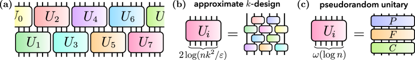
Figure 2: (a) Our random unitary ensemble corresponds to a two-layer brickwork circuit, where each small unitary acts on $2\xi$ qubits in each layer. (b) To generate $\varepsilon$-approximate unitary $k$-designs in $\log n$ depth, we draw each small unitary from an approximate unitary $k$-design on $2\xi=2\log(nk^{2}/\varepsilon)$ qubits. (c) To generate pseudorandom unitaries in $\text{poly}\log n$ depth, we draw each small unitary from a pseudorandom unitary ensemble, such as the $PFC$ ensemble [60, 65], on $2\xi=\omega(\log n)$ qubits.

At first glance, the fact that one can create random unitaries in such low depth may seem surprising. Indeed, many properties of 1D circuits, such as the light-cone volume and entanglement entropy, require at least linear depth to reach their Haar-random values. The key insight to reconcile this with our results is that such properties cannot be efficiently measured in any quantum experiment involving the random unitary $U$ [89]. For this reason, these properties do not form obstacles to realizing pseudorandom unitaries or approximate unitary designs.

2 Main Results

We now introduce our random circuit construction (Fig. 2) and present our main results characterizing the circuit depth. For simplicity, we focus at first on the simplest possible circuit geometry, a 1D line. Later, we show how to extend our construction to any geometry using graph-theoretic techniques.

Our construction organizes the $n$ qubits along a 1D line into $m$ local patches of $\xi=n/m$ qubits each. Our random unitary ensemble $\mathcal{E}$ corresponds to a two-layer circuit, in which each small random unitary acts on two neighboring patches of qubits, and the small random unitaries are arranged in a brickwork fashion between the two layers. When the small random unitaries over local patches have depth $d$ in terms of two-qubit gates, our proposed random circuit construction has circuit depth $2d$.

2.1 Random unitary designs

We can quantify how close the two-layer brickwork ensemble $\mathcal{E}$ is to an $n$-qubit Haar-random unitary using the notion of approximate unitary designs. An ensemble $\mathcal{E}$ forms an approximate unitary $k$-design if it approximates the Haar ensemble $H$ up to the $k$-th moment. The gold standard for quantifying the approximation error is given in [50]: A random unitary ensemble $\mathcal{E}$ forms an $\varepsilon$-approximate unitary $k$-design if the following holds,

$$(1-\varepsilon)\,\Phi_{H}\,\preceq\,\Phi_{\mathcal{E}}\,\preceq\,(1+\varepsilon)\,\Phi_{H},$$ (2.1)

where the quantum channel $\Phi_{\mathcal{E}}(\cdot)$ is defined via

$$\Phi_{\mathcal{E}}(A)\coloneqq\operatorname*{{\mathbb{E}}}_{U\sim\mathcal{E}}\left[U^{\otimes k}AU^{\dagger,\otimes k}\right],$$ (2.2)

and similarly for the Haar ensemble. Here, $\Phi\preceq\Phi^{\prime}$ denotes that $\Phi^{\prime}-\Phi$ is a completely-positive map. The error $\varepsilon$ is commonly known as the relative error or multiplicative error. Operationally, the relative error guarantees that any quantum experiment that involves $k$ queries to a unitary $U$ sampled from $\mathcal{E}$, produces an output state that is $2\varepsilon$-close in trace distance to the output state when $U$ is sampled from the Haar ensemble; see Appendix B.1.

Let us assume that each small random unitary in the two-layer brickwork ensemble $\mathcal{E}$ is drawn randomly and independently from an $\frac{\varepsilon}{n}$-approximate unitary $k$-design on $2\xi$ qubits. Our main result is that $\mathcal{E}$ forms an $\varepsilon$-approximate unitary $k$-design whenever the number $\xi$ of qubits in each local patch is at least logarithmic in $n,k$ and $\varepsilon^{-1}$.

Theorem 1 (Gluing small random unitary designs).

Given any approximation error $\varepsilon\leq 1$. Suppose each small random unitary in the two-layer brickwork ensemble $\mathcal{E}$ is drawn from an $\frac{\varepsilon}{n}$-approximate unitary $k$-design on $2\xi$ qubits with circuit depth $d$. Then $\mathcal{E}$ forms an $\varepsilon$-approximate unitary $k$-design on $n$ qubits with depth $2d$, whenever the local patch size is at least $\xi\geq\log_{2}(nk^{2}/\varepsilon)$.

We describe the main ideas and technical lemmas behind the theorem in Section 4 and Fig. 5. The proof details are provided in Appendix B.3.

By utilizing existing constructions of random unitary designs to instantiate each small random unitary, Theorem 1 immediately allows us to construct designs in very low depth.

Corollary 1 (Low-depth random unitary designs).

Random quantum circuits over $n$ qubits can form $\varepsilon$-approximate unitary $k$-designs in circuit depth

• $d=\mathcal{O}\big{(}\!\log\left(n/\varepsilon\right)\cdot k\,\mathrm{poly}\log(k)\big{)}$, for 1D circuits without ancilla qubits,

• $d=\mathcal{O}\big{(}\!\log\log(n/\varepsilon)\big{)}$, for all-to-all circuits with $\mathcal{O}(n\log(n/\varepsilon))$ ancilla qubits and $k\leq 3$.

For general $k$, we take each small unitary to be a 1D local random circuit on $2\xi$ qubits, which form $\frac{\varepsilon}{n}$-approximate $k$-designs in depth $d=\mathcal{O}((k\xi+\log(n/\varepsilon))\,\text{poly}\log k)$ [62]. For $k\leq 3$, we take each small unitary to be a random Clifford unitary [90, 91], which can be implemented in depth $d=\mathcal{O}(\log\xi)$ using ancilla qubits and non-local two-qubit gates [92, 93]. In both cases, our result exponentially improves the system size $n$ dependence over all known constructions. We provide a detailed discussion and additional constructions in Appendix B.4.

Finally, we confirm that the system size $n$ dependence of our approximate unitary designs is optimal for both 1D circuits and general all-to-all circuit architectures.

Proposition 1.

(Depth lower bound for unitary designs) Any quantum circuit ensemble over $n$ qubits that forms an approximate unitary $2$-design requires circuit depth

• $d=\Omega\big{(}\!\log n\big{)}$, for 1D circuits with any number of ancilla qubits,

• $d=\Omega\big{(}\!\log\log n\big{)}$, for all-to-all circuits with any number of ancilla qubits.

The proposition follows by analyzing the output distribution when a state $U\ket{0^{n}}$ is measured in a random product basis. When $U$ has too low of a depth, the output distribution features large fluctuations in its low-weight marginals that differ from those of a Haar-random unitary (Appendix B.5).

2.2 Pseudorandom unitaries

We can also quantify how close $\mathcal{E}$ is to a Haar-random unitary using the concept of a pseudorandom unitary (PRU) [47, 60, 59]. Pseudorandom unitaries are random unitary ensembles that are indistinguishable from the Haar-random ensemble by any efficient quantum algorithm that can query $U$ for any number of times. In more detail, an $n$-qubit pseudorandom unitary is secure against a $t(n)$-time adversary if it is indistinguishable from a Haar-random unitary by all $t(n)$-time quantum algorithms. A formal introduction to pseudorandom unitaries is provided in Appendix C.

While several constructions of pseudorandom unitaries have been proposed [47, 60, 59], thus far their security has only been shown for non-adaptive quantum algorithms. Thus, the existence of pseudorandom unitaries has remained a conjecture. This conjecture is recently resolved in Ref. [65] using the so-called $PFC$ construction proposed in Ref. [60]. Here, $P$ is a quantum-secure pseudorandom permutation, $F$ is a quantum-secure pseudorandom function, and $C$ is a random Clifford unitary. Assuming no subexponential-time quantum algorithm can solve the Learning With Errors (LWE) problem [94], one can efficiently construct $P$ and $F$ such that they are indistinguishable from a truly random permutation and function by any subexponential-time quantum adversary [95, 96]. The analysis in Refs. [65] then shows that $PFC$ is a pseudorandom unitary with security against any subexponential-time quantum adversary. This $n$-qubit PRU can be implemented in circuit depth $\operatorname{poly}(n)$ in 1D circuits and $\operatorname{poly}\log(n)$ in all-to-all circuits.

To construct pseudorandom unitaries with even lower circuit depth, let us draw each small random unitary in the two-layer brickwork ensemble $\mathcal{E}$ from a PRU ensemble on $2\xi$ qubits, and set $\xi=\omega(\log n)$. We assume each small unitary is secure against $\operatorname{poly}(n)$-time quantum adversaries. Since $\xi=\omega(\log n)$, a $\operatorname{poly}(n)$-time adversary is an $\exp(o(\xi))$-time adversary; hence, this is automatically satisfied by drawing each small unitary from a PRU ensemble with subexponential security, as above. Our main finding is that the resulting ensemble $\mathcal{E}$ is an $n$-qubit pseudorandom unitary ensemble.

Theorem 2 (Gluing small pseudorandom unitaries).

Let $n$ be the number of qubits in the whole system and $\xi=\omega(\log n)$ be the number of qubits in each local patch. Suppose each small random unitary in the two-layer brickwork ensemble $\mathcal{E}$ is a $2\xi$-qubit pseudorandom unitary secure against $\operatorname{poly}(n)$-time adversaries. Then $\mathcal{E}$ forms an $n$-qubit pseudorandom unitary secure against $\operatorname{poly}(n)$-time adversaries.

An overview of our proof is provided in Section 4, and details are given in Appendix C.3.

Using the $PFC$ construction [60, 65] to instantiate each small random unitary, we obtain $n$-qubit pseudorandom unitaries in the following low circuit depths. A detailed proof is given in Appendix C.4.

Corollary 2 (Low-depth pseudorandom unitaries).

Under the conjecture that no subexponential-time quantum algorithm can solve LWE, random quantum circuits over $n$ qubits can form pseudorandom unitaries secure against any polynomial-time quantum adversary in circuit depth

• $d=\mathrm{poly}\log n$, for 1D circuits,

• $d=\mathrm{poly}\log\log n$, for all-to-all circuits.

Our depth scaling improves exponentially over all known proposals for pseudorandom unitaries [47, 60, 59, 65], which require $\mathrm{poly}(n)$-depth for 1D circuits and $\mathrm{poly}\log(n)$-depth for general circuits.

As in the previous section, our scaling of the depth is in fact optimal. This follows from recent work on shallow quantum circuits, which provides a polynomial-time algorithm to learn any 1D circuit of depth $\mathcal{O}(\log n)$, and any general circuit of depth $\mathcal{O}(\log\log n)$ [97]. If one can learn a circuit, one can trivially distinguish it from a Haar-random unitary. Thus, 1D circuits require $\mathrm{poly}\log n$ depth to form PRUs, and general circuits require $\mathrm{poly}\log\log n$ depth. We remark that the precise polynomial degree in Corollary 2 depends on the specific LWE problem one conjectures to be hard.

Figure 3: (a) Shallow random classical circuits cannot look uniformly random. In contrast, our results show that shallow random quantum circuits can already look Haar-random. (b) To create random unitaries on any circuit geometry, we implement a 1D random circuit along a Hamiltonian path of the geometry. While Hamiltonian paths do not exist in any geometry, when jumping to constant-distance neighbor is allowed, they always exist and are efficient to construct.

2.3 Comparison between quantum and classical reversible circuits

To gain a better intuition for our findings, it is helpful to contrast our results on random quantum circuits with the behavior of random classical circuits [Fig. 3(a)]. A classical reversible circuit over $n$ bits corresponds to a permutation on the $2^{n}$ bitstrings, $\{0,1\}^{n}$. To determine how quickly a classical circuit can resemble a random permutation, let us consider the output of such a circuit when applied to two input bitstrings, $b_{0},b_{1}\in\{0,1\}^{n}$, that differ only in their first bit. For these inputs, a random permutation will output two bitstrings with almost no correlation between them. In contrast, any classical circuit with depth less than $n/4$ in 1D, or less than $\log_{2}(n/4)$ in all-to-all circuits, will produce two output strings that are identical on $3n/4$ bits. This follows because the light-cone of the first bit has size at most $n/4$. Hence, to match even the second moment of a random permutation, reversible classical circuits require depth $d=\Omega(n)$ in 1D, and $d=\Omega(\log n)$ in all-to-all circuits. These classical circuit depths are exponentially larger than our obtained quantum circuit depths.

Physically, this exponential reduction in the quantum circuit depth is made possible by the abundance of non-commuting observables in quantum mechanics. To distinguish a classical or quantum circuit from a random permutation or unitary, an observer must eventually measure the state of the system in some chosen basis. In a classical circuit, all observables commute. Thus, information about input bits far from the first bit can only scramble into observables that commute with the measurement basis (i.e. the computational basis). This causes the information to impact the measurement results, which allows the observer to easily distinguish whether two input strings have the same values far from the first bit.

In contrast, quantum circuits are able to locally hide information into non-commuting observables. When applied to a quantum state within an experiment, a random unitary from our ensemble will scramble information about the quantum state over local regions of $4\xi$ qubits. There are a large number, $e^{\mathcal{O}(\xi)}$, of observables on these qubits that information can scramble into; moreover, most of these observables do not commute with one another. This means that it is exceedingly unlikely that the randomly scrambled information will be contained in observables that commute with the observer’s measurement basis. This causes the measurement outcome to become nearly independent of details about the initial quantum state, in such a way that the unitary appears Haar-random. In this manner, non-commuting observables allow quantum circuits to appear quantumly random exponentially faster than classical circuits can appear classically random.

2.4 Creating random unitaries on any geometry

We provide two methods to extend our construction from 1D circuits to any circuit geometry (see Appendix D for complete details). We consider a geometry to be any connected bounded-degree graph, where each qubit is a node on the graph and two nodes are connected by an edge if one can implement a two-qubit gate between the two qubits [98, 99]. This graph-theoretic definition includes all common physical geometries, such as a 1D circle, a 3D plane, a torus, a binary tree, a hyperbolic space, and a highly connected expander graph.

Our first method shows that a depth-$d$ quantum circuit on a 1D line can be implemented on any geometry in circuit depth $\mathcal{O}(d)$. We do so by efficiently constructing a Hamiltonian path that goes through every node in the graph of the geometry exactly once. Although a Hamiltonian path does not always exist and is generally hard to find, we show that when one allows jumps to a constant-distance neighbor on the graph, a Hamiltonian path always exists and can be found efficiently [Fig. 3(b)]. The two-qubit gates between constant-distance neighbors can then be implemented using a carefully-designed swap network. Our second method extends Theorem 1 to general two-layer brickwork circuits. This allows one to glue together small random unitaries on a wide variety of geometries of interest, such as a 2D circuit consisting of many overlapping squares [Fig. 5(c)]. Both methods apply both to our construction of low-depth unitary designs and low-depth PRUs.

3 Applications

Let us now turn to applications of our results. We summarize a handful of the most prominent applications below, and provide full details in Appendix E.

Provably-efficient shallow classical shadows: Classical shadow estimation utilizes random measurements to achieve rapid estimations of many non-commuting observables [19]. Traditionally, these measurements utilize random Clifford unitaries on $n$ qubits, which require a linear circuit depth to implement. In Appendix E.1, we show that these deep Clifford unitaries can be replaced by Clifford circuits with $\log n$ depth from our construction, while retaining essentially the same guarantees on the protocol’s sample complexity. This depth scaling confirms prior conjectures in Refs. [67, 69].

A key motivation for these shallow shadow protocols is to address experimental limitations due to noise in quantum devices. To this end, we provide a rough estimate for the number of qubits that can be reached with our shallow circuit construction as opposed to the traditional approach. For leading current noise rates $\gamma\approx 0.5\%$, one can perform roughly $1/\gamma\approx 200$ circuit gates to within good many-body fidelity. With linear-depth Clifford circuits, this limits shadow tomography to small numbers of qubits, $n\approx 15$ (i.e. $n^{2}\approx 200$). On the other hand, our approach opens the door to high-fidelity shadow estimation on up to $n\approx 40$ qubits (i.e. $n\log_{2}n\approx 200$). Due to its favorable scaling, the advantage of our approach will become even more stark as noise rates improve.

Quantum hardness of recognizing topological order: The detection of topologically-ordered phases of matter has remained a notoriously difficult challenge across both materials and atomic, molecular, and optical experiments [77, 78, 79, 80, 81, 82, 83, 84, 85, 86, 87, 88]. From a quantum information perspective, one of the defining features of topological order is its invariance under the application of any low-depth local unitary circuit [74, 75, 76]. From this defining property, we apply Corollary 2 to prove that recognizing topological order is, in fact, quantumly hard at any poly-logarithmic depth (Appendix E.2):

Corollary 3 (Hardness of recognizing topological order).

Consider any definition of topological order such that (i) the product state has trivial order and the toric code state has non-trivial topological order, and (ii) the topological order of these states is preserved under any depth-$\ell$ geometrically-local circuit. Then, recognizing topological order is quantum computationally hard for any $\ell=\Omega(\mathrm{poly}\log n)$.

The criteria of the corollary apply to nearly every existent definition of topological order [100].

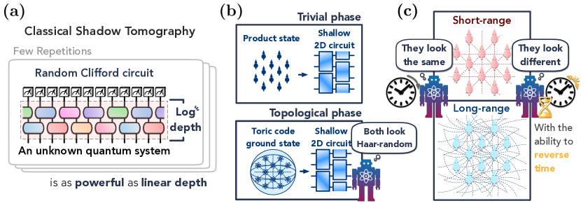
Figure 4: The low-depth unitary designs and pseudorandom unitaries that we construct have broad applications, several of which are depicted here. (a) Log-depth classical shadows: Our shallow unitary 3-designs enable provably-efficient classical shadow tomography using $\log(n)$-depth random Clifford circuits instead of linear depth. (b) Quantum hardness of recognizing topological order: By applying our shallow pseudorandom unitaries to product and toric code states, we generate pseudorandom states with trivial and topological order, respectively. This demonstrates that recognizing topological order in an unknown state is quantumly hard. (c) Power of time-reversal in learning: We establish that quantum experiments capable of reversing time-evolution can exhibit super-polynomial advantages over conventional experiments. We prove this in a simple example where one wishes to detect whether long-range couplings are present in a strongly-interacting dynamical quantum system.

Quantum advantage for learning low-complexity quantum systems: Our results immediately imply that several well-known quantum learning advantages [101, 102, 103, 104] that so far only apply to highly-complex systems also hold in low-complexity systems. A particularly relevant example concerns the task of distinguishing a random unitary process from a fully depolarizing channel [103, 104]. This can be solved efficiently by an observer with quantum access to the process of interest, but requires super-polynomially many queries for any classical observer [103, 104]. Thus far, this advantage has only been known for Haar-random unitaries, which require $\exp(\mathcal{O}(n))$ circuit depth and are thus poor models for quantum processes encountered in the physical world. Our results show that this separation holds computationally for circuits with double-exponentially smaller depth, $\text{poly}\log n$. Moreover, we show a similar quantum-classical separation for learning the entanglement structure of states generated by shallow quantum circuits. We refer to Appendix E.3 for additional details.

The power of time-reversal in learning: Leveraging an assortment of interaction engineering techniques, many modern quantum experiments have the ability to time-reverse their dynamics [105, 106, 107, 108, 109, 110, 111, 112, 113, 114]. One surprising application of our results is to show that such experiments allow one to learn properties of quantum dynamics exponentially more efficiently than conventional experiments without time-reversal [115, 116]. We demonstrate this in a simple physically-motivated example. Suppose one wishes to detect whether a quantum circuit contains only local interactions (e.g. in 2D), or instead, a combination of local interactions and small long-range couplings. From Corollary 2, this task is immediately hard for circuits with poly-logarithmic depth, since at such depths one cannot distinguish either circuit from a Haar-random unitary. On the other hand, in Appendix E.4, we show that this task is easy for experiments that can implement both the circuit $U$ and its time-reverse $U^{\dagger}$. This follows from standard measurement protocols for so-called out-of-time-order correlors [117, 118, 119, 120, 121]. We remark that this separation is intrinsically quantum mechanical, by similar light-cone arguments as below Theorem 1.

Output distributions of random quantum circuits: Random circuit sampling (RCS) is a leading current candidate for quantum computational supremacy [22]. Hardness results on RCS typically rely on two ingredients: worst-case hardness, and anti-concentration of the random circuits’ output distributions [122, 23, 24]. Thus far, these two ingredients have only coincided in relatively deep, $d=\Omega(\sqrt{n})$, 2D random circuits [123, 55]. Our construction of approximate unitary 2-designs [Fig. 2(c)] yields a 2D random circuit ensemble with anti-concentration and worst-case hardness in depth $\log n$. We can also prove several stronger statements about the output distributions of random quantum circuits by building upon our approximate $k$-designs for larger $k$. Namely, we show that, at depth $\Omega(\log n)$, the output distributions of random circuits are far-from-uniform with probability close to one, and that at depth $\mathrm{poly}\log(n)$, the output distributions are both far-from-uniform and yet computationally-indistinguishable from the uniform distribution; see Appendix E.5.

4 Proof overview

In this section, we overview the key ideas that lead to our proofs of Theorems 1, 2 and Proposition 1. We refer to the Appendix for full details of each proof.

4.1 Gluing small random unitary designs (Theorem 1)

Our proof proceeds in several steps. As the first step, we utilize a technical lemma that bounds the relative error $\varepsilon$ [see Eq. (2.1)] of any approximate unitary $k$-design in terms of its additive error when applied to the EPR state. The proof is given in Appendix B.2.2.

Lemma 1 (Unitary designs from EPR states).

A random unitary ensemble $\mathcal{E}$ acting on an $n$-qubit Hilbert space $\mathcal{H}$ forms an $\varepsilon$-approximate unitary $k$-design with error

$$\varepsilon=\frac{4^{nk}}{k!}\cdot\left(1+\frac{k^{2}}{2^{n+1}}\right)\cdot\big{\lVert}\,[(\Phi_{\mathcal{E}}-\Phi_{H})\otimes\mathbbm{1}](P^{\mathrm{EPR}})\,\big{\rVert}_{\infty},$$ (4.1)

where $P^{\mathrm{EPR}}$ is the projector onto the EPR state on $\mathcal{H}^{\otimes k}\otimes\mathcal{H}^{\otimes k}$.

The lemma is useful because bounding the additive error is, in most cases, substantially easier than bounding the relative error. We note that the lemma improves existing bounds [50] by a factor of $k!$. This factor of $k!$ improvement is essential for our construction of low-depth pseudorandom unitaries, in which we take $k$ to be superpolynomial in $n$.

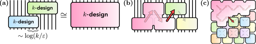
Figure 5: (a) A key step in our proof is to show that one can “glue” two approximate unitary $k$-designs into a larger $\varepsilon$-approximate unitary $k$-design. This holds whenever the two unitaries are applied in sequence and overlap on at least $\sim\!\text{log}(k/\varepsilon)$ qubits. (b) To prove Theorems 1, 2, we apply this gluing lemma $n/\xi$ times as shown (arrows). At each application, we glue one additional small unitary (green) into a larger unitary design on all qubits to its left (pink). (c) The gluing lemma also enables us to immediately extend our theorems to 2D circuits, by applying the lemma in the order shown (arrows), as well as other geometries.

The second step in our proof arrives at the critical difference between quantum and classical circuits. We show that one can “glue” two unitary designs together to form a larger unitary design, as long as the two unitaries overlap on a relatively small number of qubits; see Fig. 5(a).

Lemma 2 (Gluing two random unitaries; informal).

Let $A$, $B$, $C$ be three disjoint subsystems. Consider a random unitary given by $V_{ABC}=U_{AB}U_{BC}$, where $U_{AB}$ and $U_{BC}$ are drawn from $\varepsilon_{1}$ and $\varepsilon_{2}$-approximate unitary $k$-designs, respectively. Then $V_{ABC}$ is an $\varepsilon$-approximate unitary $k$-design with

$$1+\varepsilon\leq(1+\varepsilon_{1})(1+\varepsilon_{2})\left(1+\frac{5k^{2}}{2^{|B|}}\right),$$ (4.2)

as long as the number of qubits in $B$ satisfies $|B|\geq\log_{2}(5k^{2})$.

In classical circuits, such a lemma cannot exist because any two input bitstrings that differ only on $A$ would have outputs that do not differ on $C$. In quantum circuits, this is not an issue, because information on $C$ is scrambled into random non-commuting observables. As long as $|B|\gtrsim\log(k/\varepsilon)$, this information is effectively hidden from any quantum experiment [124].

Our proof of Lemma 2 follows relatively quickly upon expressing the state in Lemma 1 in terms of permutation operators that act on $\mathcal{H}^{\otimes k}$. Applying the standard formula for the twirl over a unitary $k$-design [125], we find (see Appendix B.3.2 for full details)

$$[\Phi_{\mathcal{E}}\otimes\mathbbm{1}](P^{EPR})=2^{-nk}\sum_{\sigma,\tilde{\sigma},\tau,\tilde{\tau}}\text{Wg}_{\sigma,\tau}(2^{|B|+|C|})\,G_{\tau,\tilde{\sigma}}(2^{|B|})\,\text{Wg}_{\tilde{\sigma},\tilde{\tau}}(2^{|A|+|B|})\,\big{[}\tilde{\tau}_{AB}\tau_{C}\otimes\tilde{\sigma}_{A}\sigma_{BC}\big{]},$$ (4.3)

where $\sigma,\tau\in S_{k}$ and $\tilde{\sigma},\tilde{\tau}\in S_{k}$ are permutation operators arising from the twirl over $U_{BC}$ and $U_{AB}$, respectively, in Lemma 2. Here, the Gram matrix, $G_{\sigma,\tau}(D)=\text{tr}(\sigma\tau^{-1})$ is equal to the inner products of permutation operators, and the Weingarten matrix, $\text{Wg}_{\sigma,\tau}(D)$, is the inverse of the Gram matrix. Crucially, when the Hilbert space dimension $D$ is large, the permutation operators are approximately orthogonal to one another [55]. This implies that the Gram and Weingarten matrices are nearly proportional to the identity, $G_{\sigma,\tau}(D)\approx D^{k}\cdot\mathbbm{1}_{\sigma,\tau}$ and $\text{Wg}_{\sigma,\tau}(D)\approx D^{-k}\cdot\mathbbm{1}_{\sigma,\tau}$, up to small corrections of order $\mathcal{O}(k^{2}/D)$. In this limit, the only terms that contribute to Eq. (4.3) obey $\sigma=\tau=\tilde{\sigma}=\tilde{\tau}$. However, these are exactly the same terms that appear when twirling over a Haar unitary on the entire system $ABC$. By making this intuition precise, we bound the operator norm in Lemma 1 and thus show that the ensemble forms an approximate unitary design.

Our proof of Theorem 1 follows immediately from Lemma 2. We proceed unitary-by-unitary from left to right as in Fig. 5(b). At each step, we apply Lemma 2 to glue the next unitary into a large design formed by all of the preceding unitaries. After $m-2$ steps, this produces an approximate design on all $n$ qubits. The design has relative error

$$\approx(m-1)\cdot\frac{\varepsilon}{n}+(m-2)\cdot\frac{5k^{2}}{2^{\xi}},$$ (4.4)

since there are $m-1$ small random unitaries, each drawn from an $\frac{\varepsilon}{n}$-approximate $k$-design, and we applied Lemma 2 a total of $m-2$ times. Setting $\xi=\Omega(\log_{2}(nk^{2}/\varepsilon))$ and recalling $\xi=n/m$ gives Theorem 1. We refer to Appendix B.3 for a detailed proof including tight constant factors.

4.2 Depth lower bound for unitary designs (Proposition 1)

To lower bound the depth of any approximate unitary 2-design, we apply a random unitary from the ensemble to the zero state, and consider the output distribution, $p_{U,v}(x)=|\bra{x}v^{\dagger}U\ket{0^{n}}|^{2}$, when the resulting state, $U\ket{0^{n}}$, is measured in a random product basis, $\{v\ket{x}\}$. Here $v$ is a tensor product of random single-qubit unitaries, and $x\in\{0,1\}^{n}$. When $U$ is Haar-random, the distribution is nearly flat across the $2^{n}$ basis states. This implies that the expected collision probability, $\mathbbm{E}_{U,v}[\sum_{x}p_{U,v}(x)^{2}]\approx 2/2^{n}$, is almost maximally small. Since the collision probability corresponds to the expectation value of a positive operator, $\mathbbm{E}_{v}[\sum_{x}(v\outerproduct{x}{x}v^{\dagger})^{\otimes 2}]$, in the state $\Phi_{\mathcal{E}}(\outerproduct{0^{n}}{0^{n}}^{\otimes 2})$, this small value must be replicated by any approximate unitary 2-design.

Let us now analyze what happens when $U$ has too low a depth. We will track how local information about the initial state $\ket{0^{n}}$ affects the distribution $p_{U,v}(x)$. Consider the $n$ single-qubit stabilizers of $\ket{0^{n}}$. Each stabilizer can scramble to at most $L$ qubits under $U$, where $L$ is the size of the light-cone of $U$. Intuitively, each scrambled stabilizer will commute with the basis of the random product measurement with probability at least $1/3^{L}$. This leads to small bias, $\Omega(1/3^{L})$, in the marginals of $p_{U,v}(x)$ that contain the stabilizer, which, we find, leads to a small increase, $\Omega(1/3^{L}\cdot 1/2^{n})$, in the collision probability. Summing over the $n$ single-qubit stabilizers, we obtain a strict lower bound on the expected collision probability, $\mathbbm{E}_{U,v}[\sum_{x}p_{U,v}(x)^{2}]\geq(n/3^{L})/2^{n}$ (see Appendix B.5 for details). For 1D circuits, the light-cone grows linearly, $L=2d$, so one requires $d=\Omega(\log n)$ to replicate the Haar collision probability. For all-to-all circuits, the light-cone grows exponentially, $L=2^{d}$, so one requires $d=\Omega(\log\log n)$.

4.3 Gluing small pseudorandom unitaries (Theorem 2)

To prove that $\mathcal{E}$ forms a pseudorandom unitary ensemble, we introduce an additional unitary ensemble, $\mathcal{E}^{*}$, in which each small random unitary in the two-layer brickwork ensemble is drawn from the Haar ensemble on $2\xi$ qubits. We establish Theorem 2 in two steps: (1) we show that $\mathcal{E}$ and $\mathcal{E}^{*}$ cannot be distinguished from one another, and (2) we show that $\mathcal{E}^{*}$ and the $n$-qubit Haar ensemble also cannot be distinguished. The proof of Theorem 2 is complete after combining claims (1) and (2).

Intuitively, claim (1) follows because each small pseudorandom unitary in $\mathcal{E}$ cannot be distinguished from a small Haar-random unitary by any $\operatorname{poly}(n)$-time adversary. To establish the claim precisely, we show that the security of the individual small PRUs also implies the security of the collection of small PRUs. We do so via a hybrid argument, where we use the fact that any quantum algorithm involving $k$ queries to a set of Haar-random unitaries can be efficiently simulated using unitary $k$-designs, despite the fact that Haar-random unitaries have exponential circuit complexity.

To establish claim (2), we apply Theorem 1 to compare $\mathcal{E}^{*}$ and the $n$-qubit Haar ensemble. Note that each small Haar-random unitary in $\mathcal{E}^{*}$ is trivially a $0$-approximate unitary $\infty$-design. Therefore, by Theorem 1, $\mathcal{E}^{*}$ is an $\varepsilon$-approximate unitary $k$-design for any $\varepsilon,k$ such that $\log_{2}(nk^{2}/\varepsilon)\leq\xi$. To complete the proof, we note that any $\varepsilon$-approximate unitary $k$-design is indistinguishable from a Haar-random unitary by $\operatorname{poly}(n)$-time adversaries, as long as $\varepsilon=1/\exp(\omega(\log n))$ is smaller than any inverse-polynomial function in $n$, and $k=\exp(\omega(\log n))$ is larger than any polynomial function in $n$. We achieve such $\varepsilon,k$ whenever $\xi=\omega(\log n)$. For such $\xi$, no $\operatorname{poly}(n)$-time quantum algorithm can distinguish between $\mathcal{E}^{*}$ and the $n$-qubit Haar ensemble, establishing claim (2). We emphasize that this claim requires taking $k$ to be superpolynomial in $n$, and hence the $\log k$ dependence in Lemma 2, achieved using Lemma 1, instead of a $\mathrm{poly}(k)$ dependence is crucial to establish Theorem 2.

5 Discussion

We have shown that random unitaries can be naturally generated in extremely low circuit depths. Our results reveal a surprising and profound property of quantum circuits, which differs fundamentally from classical systems. Moreover, our construction of random unitaries is both exceptionally simple and highly versatile, from either an experimental or theoretical perspective. We showcase these features by applying our results to a handful of prominent applications across quantum science, including: rigorous guarantees for classical shadows with log-depth Clifford circuits, strict lower bounds on the complexity of detecting many-body topological phases, quantum advantages for learning low-complexity physical systems, improved bounds on the output distributions of quantum supremacy circuits, and an exponential separation between quantum experiments that have access to forward time-evolution, $U$, and those that have access to both $U$ and its time-reversal, $U^{\dagger}$.

Our results open up numerous avenues for future work. Most importantly, we expect that the list of applications explored in our work is far from exhaustive. Random unitaries are a ubiquitous tool in quantum information theory and in understanding complex quantum processes. In quantum benchmarking, efficient learning using random unitaries extends to fermionic, bosonic, and Hamiltonian systems [20, 126, 127, 128, 33, 129, 130]. Can one show that the formation of random unitaries in extremely short times applies to these systems as well? In quantum gravity, a widespread conjecture states that black holes are the fastest scramblers in nature [38]. If we consider scrambling to be the formation of random unitary designs, could the surprisingly fast formation of designs on any geometry found in our work provide new insight into quantum black holes and the AdS/CFT correspondence [131, 132, 133]?

On the mathematical side, an obvious open question concerns the optimality of our unitary design construction. While we have proven in Proposition 1 that our $n$-dependence is optimal, and we inherit the optimal $k$-dependence of Ref. [62] up to polylogarithmic factors, the relation between these two dependencies is not known. More precisely, we cannot yet rule out the possibility that $\varepsilon$-approximate unitary $k$-designs over $n$ qubits can be created in depth $\mathcal{O}(k)+\mathcal{O}(\log(n/\varepsilon))$, whereas our construction requires a depth of $\tilde{\mathcal{O}}(k)\times\mathcal{O}(\log(n/\varepsilon))$. Achieving a matching upper and lower bound on the circuit depth with respect to all three parameters $n,k,\varepsilon$ remains an outstanding challenge.

Lastly, it would be interesting to determine whether the same design depth applies to brickwork local random circuits with independent and identically-distributed gates. When we insert local random circuits into each small random unitary in our construction (as in Corollary 1), we obtain a local random circuit on a brickwork architecture, but with a small subset of the gates set to the identity. Intuitively, it seems unlikely that drawing these gates from the Haar measure on $\mathrm{SU}(4)$ would increase the depth at which random quantum circuits converge to designs, but we cannot rule this out. In fact, this suggests a more general open question: Is it possible for the deletion of random quantum gates to speed up the formation of unitary designs? This question was also raised in Ref. [55] relating to so-called censoring inequalities in Markov chains.

Acknowledgments:

We are grateful to Eric Anschuetz, Ryan Babbush, Christian Bertoni, Adam Bouland, Sergio Boixo, Fernando Brandão, Xie Chen, Soonwon Choi, Jordan Cotler, Jens Eisert, Bill Fefferman, David Gosset, Soumik Goush, Patrick Hayden, Nicholas Hunter-Jones, Marios Ioannou, Matteo Ippoliti, Vedika Khemani, William Kretschmer, Dominik Kufel, Fermi Ma, Jarrod R. McClean, Tony Metger, Ramis Movassagh, Quynh Nguyen, Mehdi Soleimanifar, Nathanan Tantivasadakarn, Umesh Vazirani, and Norman Yao for valuable discussions and insights. We would like to thank Soonwon Choi in particular for introducing TS and JH to each other, which was vital for this work. Part of this work was conducted while JH and HH were visiting the Simons Institute for the Theory of Computing. TS acknowledges support from the Walter Burke Institute for Theoretical Physics at Caltech. JH acknowledges funding from the Harvard Quantum Initiative. HH acknowledges the visiting associate position at the Massachusetts Institute of Technology. The Institute for Quantum Information and Matter, with which TS and HH are affiliated, is an NSF Physics Frontiers Center.

Note added: We extend our gratitude to Nicholas LaRacuente and Felix Leditzky for bringing their independent concurrent work on unitary designs [134] to our attention. Their approach, motivated by quantum communication, demonstrates that approximate $k$-designs can be created across two parties by exchanging only $\mathcal{O}(k\log k)$ qubits, independent of system size. Building on this, they showed that $n$-qubit $k$-designs can be generated in $\tilde{\mathcal{O}}(k^{2})\log(n)$ depth. Our work employs different constructions and analyses, yielding additional findings on low-depth pseudorandom unitaries that require an improved $\mathcal{O}(\log k)$ qubit scaling. We also provide circuit depth lower bounds and explore applications in classical shadows, quantum advantages, and many-body physics.

Appendices

We provide a road map to help the readers navigate through our appendices. Appendix A presents a brief literature review of existing results relevant to this work. Appendix B establishes our main results regarding random unitary designs. Appendix C establishes our results regarding pseudorandom unitaries. Appendix D shows how to generalize our results from 1D circuits to any circuit geometry. Finally, Appendix E presents the technical details of the applications considered in the main text.

Contents

1. 1 Introduction
2. 2 Main Results
   1. 2.1 Random unitary designs
   2. 2.2 Pseudorandom unitaries
   3. 2.3 Comparison between quantum and classical reversible circuits
   4. 2.4 Creating random unitaries on any geometry
3. 3 Applications
4. 4 Proof overview
   1. 4.1 Gluing small random unitary designs (Theorem 1)
   2. 4.2 Depth lower bound for unitary designs (Proposition 1)
   3. 4.3 Gluing small pseudorandom unitaries (Theorem 2)
5. 5 Discussion
6. A Literature review
   1. A.1 Unitary designs
   2. A.2 Pseudorandom states and unitaries
   3. A.3 Classical shadows with low-depth random circuits
   4. A.4 Recognizing topological order
   5. A.5 Quantum advantage in learning from experiments
   6. A.6 The power of time-reversal in learning
7. B Random unitary designs
   1. B.1 A brief review of approximate unitary designs
      1. B.1.1 Definitions
      2. B.1.2 Operational meaning
   2. B.2 A brief review of Haar random unitaries
      1. B.2.1 Permutation operators and the Weingarten calculus
      2. B.2.2 The Schur-Weyl duality
   3. B.3 Proof of Theorem 1: Gluing small random unitary designs
      1. B.3.1 Residual of the Haar twirl
      2. B.3.2 Gluing two random unitaries
      3. B.3.3 Completing the proof of Theorem 1
   4. B.4 Proof of Corollary 1: Low-depth random unitary designs
   5. B.5 Proof of Proposition 1: Lower bounds for unitary designs
8. C Pseudorandom unitaries
   1. C.1 Definition of pseudorandom unitaries
   2. C.2 The $PFC$ construction for pseudorandom unitaries
   3. C.3 Proof of Theorem 2: Gluing small pseudorandom unitaries
   4. C.4 Proof of Corollary 2: Low-depth pseudorandom unitaries
9. D Creating random unitaries on any geometry
   1. D.1 From 1D lines to any geometry
   2. D.2 Extension of Theorem 1 to general two-layer circuits
10. E Applications
    1. E.1 Classical shadows with 1D log-depth Clifford circuits
    2. E.2 Proof of Corollary 3: Quantum hardness of recognizing topological order
    3. E.3 Quantum advantage in learning low-complexity physical systems
       1. E.3.1 Distinguishing random pure states from maximally mixed states
       2. E.3.2 Distinguishing random unitary channels from completely depolarizing channels
       3. E.3.3 Distinguishing entangled states from unentangled states
    4. E.4 The power of time-reversal in learning
    5. E.5 Output distributions of shallow quantum circuits

Appendix A Literature review

A.1 Unitary designs

Unitary designs [44, 45, 46] are a ubiquitous tool throughout quantum information. Early work [48] established that local random quantum circuits can form approximate unitary $2$-designs in depth $\mathcal{O}(n+\log(1/\varepsilon))$. This was shown by proving the existence of a gap in the spectrum of the moment operators, $\operatorname*{{\mathbb{E}}}[U^{\otimes k}\otimes\overline{U}^{\otimes k}]$, for $k=2$. Later work [49] provided evidence for such a gap at higher $k$ using a mean-field analysis, in which the moment operators can be interpreted as frustration-free Hamiltonians. Using techniques to bound spectral gaps of quantum-many body systems, Brandão, Harrow and Horodecki [50] proved that local random quantum circuits indeed generate approximate unitary $k$-designs in depth $\mathcal{O}(k^{9.5}(nk+\log(1/\varepsilon))$ for any $k$.

Since these seminal early works, a tremendous effort has been devoted to improving the $k$ dependence of the circuit depth. To begin, Ref. [54] showed that the bound in Ref. [50] can be improved to $\mathcal{O}(k^{4+o(1)}(nk+\log(1/\varepsilon))$, where $o(1)$ goes to zero as $k\to\infty$. More recently, Ref. [61] constructed approximate unitary designs with relative error using circuits of depth $\mathcal{O}(\log(n)(nk^{2}+\log(1/\varepsilon))$ which grows only quadratically in $k$. Instead of local random circuits, Ref. [61] considered the use of random Pauli rotations, $e^{\mathrm{i}\theta P}$; these rotations can then be decomposed into local circuits if desired. Even more recently, Refs. [59, 60] constructed approximate unitary designs with depth linear in $k$; however, these constructions only achieved additive error and not relative error. (We recall that relative errors are necessary to match Haar-random behavior in any quantum experiment that adaptively queries the random unitary $k$ times; see Appendix B.1.2.) A wide array of works suggested that approximate unitary designs with relative errors can be generated in depth $\mathcal{O}(nk)$ [52, 49, 58, 51]. Finally, Ref. [62] resolved this conjecture up to poly-logarithmic factors by showing that local random quantum circuits generate $\varepsilon$-approximate unitary designs in depth $\mathcal{O}(\mathrm{poly}\log(k)(nk+\log(1/\varepsilon))$ for $k=\mathcal{O}(2^{2n/5})$.

In every case above, the circuit depth of the unitary ensemble grows linearly in $n$. For additive error designs, Ref. [55] showed that the $n$-dependence can be improved to $\mathcal{O}(n^{1/\mathcal{D}})$, if one considers local random quantum circuits on $\mathcal{D}$-dimensional lattices. Another work that focuses on the $n$-dependence is Ref. [53], which uses circuits of linear depth but only an $n$-independent number of non-Clifford gates, $\mathcal{O}(k^{4}+k\log(1/\varepsilon))$, again for additive error designs. Finally, we recall that for the specific case of Clifford unitaries and all-to-all-connected circuit architectures, exact unitary 2- and 3-designs can be generated in $\log n$ depth using ancilla qubits [92, 93].

Our work improves the $n$ dependence exponentially compared to every prior work above. Fundamentally, this is because our work is the first that does not require circuits with extensive light-cones.

A.2 Pseudorandom states and unitaries

Pseudorandom states and unitaries were introduced in Ref. [47]. Ref. [47] also provides the first examples of pseudorandom states, which assume only the existence of quantum-secure one-way functions, and provides a potential construction of pseudorandom unitaries. By assuming the quantum hardness of the Learning With Error problems [94], one can establish the existence of quantum-secure one-way functions. These quantum-secure one-way functions can then be used to construction quantum-secure pseudorandom functions [95] and quantum-secure pseudorandom permutations [96], which are important building blocks for most proposals for pseudorandom states and unitaries. Pseudorandom states and unitaries have since become a crucial concept in quantum learning theory [103, 135], cryptography [27, 136] and the AdS/CFT correspondence [133].

Towards constructing pseudorandom unitaries, Ref. [63] proved the existence of quantum pseudorandom scramblers, i.e. an ensemble of unitaries which, applied to any input state, generates an ensemble of pseudorandom states. Refs. [59, 60] constructed ensembles of unitaries that are pseudorandom with non-adaptive security. That is, such unitary ensembles are indistinguishable from the Haar ensemble by any non-adaptive polynomial-time quantum algorithm that can query $\mathrm{poly}(n)$ copies of $U$ in parallel, but only in a single round. Pseudorandom unitaries with non-adaptive security can be seen as a stronger version of quantum pseudorandom scramblers, but they still do not resolve the conjecture regarding the existence of pseudorandom unitaries. Similar to pseudorandom states [26], these works [63, 59, 60] rely on the cryptographic assumption that quantum-secure one-way functions exist in order to instantiate quantum-secure pseudorandom functions and permutations.

In an upcoming work [65], the authors resolve the conjecture regarding the existence of pseudorandom unitaries by proving that the $PFC$ construction proposed in Ref. [60] forms a pseudorandom unitary. Furthermore, Ref. [65] gives new constructions for pseudorandom unitaries that are secure against any efficient quantum algorithms that can query both the unitary $U$, its time-reversal $U^{\dagger}$, and the controlled versions of both $U$ and $U^{\dagger}$. As shown in Section 3, obtaining time-reversal in a quantum experiment is powerful. Nonetheless, Ref. [65] provides an efficient construction of pseudorandom unitaries secure against access to both time-reversal and controlled operations.

All known proposals for constructing pseudorandom states or unitaries require the implementation of pseudorandom functions or permutations. When placed in a 1D circuit layout, these require $\operatorname{poly}(n)$ depth for $n$-qubit systems. Our work provides the first construction of both pseudorandom states and pseudorandom unitaries that only requires $\operatorname{poly}\log n$ depth in 1D, which improves exponentially over all known constructions. For all-to-all-connected circuits, there are pseudorandom states that can be constructed in $\operatorname{poly}\log n$ depth [137]. For such circuits, our construction only requires circuit depth $\operatorname{poly}\log\log n$, again an exponential improvement over all known constructions of pseudorandom states and unitaries.

By building on the concept of pseudorandom states, researchers have also constructed pseudoentangled states, which are states that have low entanglement, but are computationally indistinguishable from states with high entanglement [137]. Because geometrically-local shallow quantum circuits only alter the entanglement structures of the input states up to area-law fluctuations, applying our low-depth PRUs to an initial state $\ket{\psi}$ creates pseudorandom states with almost the same entanglement structure as $\ket{\psi}$. As a special case, when $\ket{\psi}$ is any product state, applying our low-depth PRUs to $\ket{\psi}$ generates pseudoentangled states [137]. Adam Bouland has suggested to us the notion of pseudoentangling unitaries, which are unitaries that can only create short-range entanglement, but which are indistinguishable from unitaries that create volume-law entanglement. The low-depth pseudorandom unitaries we constructed are the first known construction of pseudoentangling unitaries.

A.3 Classical shadows with low-depth random circuits

Classical shadow tomography [19, 138, 102, 139, 140, 70, 72, 73] for estimating non-local observables such as fidelities requires the preparation of random Clifford unitaries. When restricted to geometrically-local circuit architectures, these random Clifford unitaries require circuits of linear depth, which limits their realization in current experiments due to the presence of noise in existing experimental platforms. Recently, multiple works [66, 67, 72, 68, 69, 141] have considered classical shadow estimation using shallow random Clifford circuits instead of linear-depth random Clifford unitaries. These proposals are known as “shallow shadows”.

It was suggested in Ref. [67] that the depth $d=\Theta(\log(n))$ achieves “an ideal middle ground” between random product measurements (depth $0$) and uniformly random Clifford unitaries (linear depth). In particular, Ref. [67] shows that random log-depth Clifford circuits reproduce the same guarantees as global Cliffords for most states drawn from a 1-design. They moreover conjectures that this scaling holds for all states. Ref. [69] proposes a physical explanation for this improvement using ideas from quantum many-body dynamics. They show that the capabilities of shallow shadows can be understood in terms of a competition between two physical processes, operator spreading and operator relaxation. Using these ideas, Ref. [69] proved that for Frobenius-normalized Pauli observables $P/\sqrt{2^{n}}$, the squared shadow norm is bounded above by $1.14^{n}$ at any circuit depth, with an optimal depth given by $\log(n)$. They conjecture that this upper bound can be further tightened to a constant at $\log(n)$ circuit depth. The conjecture is supported by numerical evidence and analytic calculations under a physically-motivated mean-field assumption, which assumes that Pauli densities on different qubits are independently identically distributed (i.i.d.) binomial random variables. However, the conjecture remains unproven due to the difficulty in formally justifying the mean-field approximation. In our work, we show that any Frobenius-norm-bounded observable, including $P/\sqrt{2^{n}}$, has a squared shadow norm of a constant at $\log(n)$ circuit depth. This resolves the conjectures posed in Refs. [67, 69].

A.4 Recognizing topological order

There exist innumerably many works across condensed matter and many-body physics on recognizing the topological order of a quantum state [80, 81, 82, 83, 84, 85, 86, 142, 143, 144, 145, 88, 146, 147, 148, 149]. In nearly all cases, the proposed approaches are heuristic and are often motivated by specific details about the quantum states that one is seeking to characterize. For example, several prominent approaches include measuring the topological entanglement entropy [86], measuring or re-constructing the expectation values of Wilson loop operators [81, 82, 146, 84, 85], and methods inspired by quantum error correction and the renormalization group [142, 149, 147]. These approaches have all been shown to succeed in small-scale numerical studies, typically involving low-entangled quantum states that are also nearby so-called “fixed points” of the topological orders of interest.

Our work shows that for even moderately more complex quantum states, all of these approaches must incur a super-polynomial overhead. In the case of the topological entanglement entropy, this is easily understood because measuring entropies in general requires an exponential sample complexity. In the case of Wilson loop and renormalization group approaches, the difficulty stems from the lack of a simple nearby fixed-point on which to begin ones’ analysis. Looking forward, several important open questions remain. Do our hardness lower bounds extend to recognizing topological phases of matter in the presence of a protecting symmetry group [76, 147]? And can we extend our results even closer to the topologically-ordered states that might arise in the physical world—e.g. what is the complexity of recognizing topological order in the ground states of 2-local Hamiltonians?

A.5 Quantum advantage in learning from experiments

Understanding how to efficiently learn from experiments is a fundamental problem in physics and has attracted significant attention recently in the quantum world. In particular, recent works have built on quantum information theory and learning theory [150] to provide rigorous theoretical foundation to understand the power and limitations in learning from quantum experiments using both classical and quantum algorithms [102, 103, 151, 88, 103, 101, 104, 152]. These efforts can be separated into two lines of work: (1) understanding the power of classical algorithms that can learn from data to solve challenging problems, and (2) proving separations between classical and quantum learning algorithms to yield rigorous quantum advantages in learning from experiments.

Ref. [152] showed that a problem can be easy to solve for a classical machine learning (ML) algorithm that can learn from quantum data even when a problem is classically-hard to solve. At a formal level, this claim is shown using the fact that training data can be viewed as a restricted form of advice strings in computational complexity theory [153], which can enhance algorithms that utilize them. Building on the computational power of data, Ref. [88] gave the first efficient classical ML algorithm to predict ground state properties from a new unseen Hamiltonian by training on a dataset collected from quantum experiments. The same problem is computationally hard for classical algorithms that do not learn from data. The sample complexity of this algorithm is $\mathcal{O}(n^{1/\epsilon})$, where $\epsilon$ denotes the prediction error. This was subsequently improved to $\log(n)e^{\mathrm{poly}\log(1/\epsilon)}$ in Ref. [154, 155] and then to $e^{\mathrm{poly}\log(1/\epsilon)}$ in Ref. [156]. When one can measure ground states of gapped quantum many-body systems, Refs. [157, 158] show that one can predict a large number of ground state properties using classical data collected from $\mathrm{poly}\log n$ local measurements. In the special case of learning states generated from shallow quantum circuits, a computationally-efficient classical algorithm to do so was developed in Ref. [97]. In addition to predicting ground states of quantum systems, Ref. [159] also showed that classical ML algorithms can efficiently predict many output state properties of arbitrary quantum processes, even when the quantum process has exponentially high complexity.

While many recent works have established the power of classical algorithms for learning from quantum experiments, a large body of work suggest that the full suite of quantum technologies can provide a significant advantage over classical methods. Refs. [103, 104, 160, 101] provide the first set of learning problems that are are easy to solve with quantum learning agents that can receive quantum information using quantum sensors, process quantum information using quantum computation, and store quantum information in quantum memory, but are provably hard to solve with classical learning agents that can receive classical information using measurements, process classical information using classical computation, and store classical information in classical memory. Refs. [103, 104] establish an exponential separation between quantum and classical learning agents for predicting highly-incompatible observables [139], performing quantum principal component analysis [161], distinguishing between the completely depolarizing channel and Haar-random unitaries [104], and learning polynomial-time quantum processes to within small average gate fidelity [103]. In Ref. [160], the authors construct a distinguishing task that is easy with access to entangled measurements over many copies of an unknown state, but hard with entangled measurements over at most $k$ copies. Refs. [151, 162] showed that some of these exponential separations become very large polynomial separations when the quantum learning agent is noisy. Finally, Refs. [163, 164, 165, 166] extended such quantum advantages to learning Pauli channels in many-qubit systems and learning displacement channels in bosonic systems.

In every existing work above, the quantum advantage is established by considering physical systems with highly non-local correlations across all $n$ qubits of the system. This is not a common condition in many physical settings, where correlation lengths are much smaller in $n$. Furthermore, in many of the learning separations above, such as distinguishing between a completely depolarizing channel and a Haar-random unitary, existing proofs require the physical system to have an exponential circuit complexity. This is also highly nonphysical. In our work, we present the first superpolynomial separation between quantum and classical agents for learning geometrically-local physical systems with correlation length $\operatorname{poly}\log n$ and circuit complexity (i.e. depth) $\operatorname{poly}\log n$.

A.6 The power of time-reversal in learning

The idea that time-reversal experiments can reveal fundamentally new aspects of many-body systems dates back to the foundations of thermodynamics [167]. The formal study of this advantage in quantum systems began in Ref. [115], which introduced a simple learning task that featured an exponential advantage in sample complexity for experiments with time-reversal over those without. However, this learning task had one significant limitation: It could also be efficiently solved without time-reversal when the experiment has access to a quantum memory. Our work significantly strengthens this separation by introducing a learning task that cannot be solved by any quantum experiment that queries $U$, including those with arbitrarily large quantum memories. Our task builds upon the physical intuition introduced in Ref. [116], which showed that time-reversal experiments are particularly advantageous for learning properties such as the connectivity of an unknown Hamiltonian.

Appendix B Random unitary designs

B.1 A brief review of approximate unitary designs

Let $\mathcal{E}$ denote an ensemble of $n$-qubit unitaries, and $\mathcal{E}_{H}$ denote the Haar-random ensemble, which samples $U$ uniformly over all $n$-qubit unitaries.

B.1.1 Definitions

A random unitary ensemble $\mathcal{E}$ forms an approximate unitary $k$-design if it approximately matches Haar-random unitaries up to the $k$-th moments. The gold standard for quantifying the approximate error in the random unitary literature [50] is given by the following.

Definition 1 (Approximate unitary design).

An ensemble $\mathcal{E}$ is an $\varepsilon$-approximate unitary $k$-design if

$$(1-\varepsilon)\,\Phi_{H}\,\preceq\,\Phi_{\mathcal{E}}\,\preceq\,(1+\varepsilon)\,\Phi_{H},$$ (B.1)

where the quantum channel $\Phi_{\mathcal{E}}(\cdot)$ is defined via

$$\Phi_{\mathcal{E}}(A)\coloneqq\operatorname*{{\mathbb{E}}}_{U\sim\mathcal{E}}\left[U^{\otimes k}AU^{\dagger,\otimes k}\right],$$ (B.2)

and similarly for the Haar ensemble. Here, $\Phi\preceq\Phi^{\prime}$ denotes that $\Phi^{\prime}-\Phi$ is a completely-positive map.

The error $\varepsilon$ in the above definition is commonly referred to as the relative error. A small relative error has an important operational meaning, in that it implies indistinguishability from a Haar-random unitary under any $k$ queries to the random unitary $U$, which we prove in Lemma 5. There also exists a weaker notion of approximation error, which we refer to as the additive error. Let $\norm{\cdot}_{\diamond}$ denote the diamond norm. The additive and relative errors are given as follows,

additive error $$\varepsilon \quad\norm{\Phi_{\mathcal{E}}-\Phi_{H}}_{\diamond}\leq\varepsilon,$$: (B.3)

relative error $$\varepsilon -\varepsilon\,\Phi_{H}\, \preceq\,\Phi_{\mathcal{E}}-\Phi_{H}\,\preceq\,\varepsilon\,\Phi_{H}.$$: (B.4)

A small relative error always implies a small additive error. However, the converse is not always true and even a superpolynomially small additive error could have a large relative error. In general, one needs to have an exponentially small additive error to guarantee a small relative error.

Lemma 3 (Additive vs relative error; Lemma 3 in Ref. [50]).

Any unitary $k$-design with relative error $\varepsilon$ is a unitary $k$-design with an additive error $2\varepsilon$. Conversely, any unitary $k$-design with additive error $\varepsilon$ is a unitary $k$-design with a relative error $2^{2nk}\varepsilon$.

We note that our work improves the latter conversion by a factor of $k!$ through Lemma 1.

B.1.2 Operational meaning

As aforementioned, there is a simple operational interpretation of the definition of approximate unitary $k$-designs. Namely, for any quantum algorithm that applies $U$ $k$ times, the output states when $U$ is sampled from $\mathcal{E}$ and when $U$ is sampled from the Haar-random ensemble $\mathcal{E}_{H}$ are close. This is captured by the following two lemmas. The first lemma states that a small additive error is equivalent to indistinguishability under $k$ nonadaptive/parallel queries to $U$.

Lemma 4 (Indistinguishability under additive error).

An approximate unitary $k$-design $\mathcal{E}$ has an additive error $\varepsilon$ if and only if for all quantum algorithms that make only one query to $U^{\otimes k}$, the output state when $U$ is sampled from $\mathcal{E}$ or from $\mathcal{E}_{H}$ is at most $\varepsilon$-far in $\norm{\cdot}_{1}$.

The second lemma states that a small relative error implies indistinguishability under any $k$ queries to $U$. These $k$ queries can depend adaptively and quantumly on all previous queries and are not restricted to querying $U$ in parallel. Hence, a small relative error is operationally much stronger than a small additive error.

Lemma 5 (Indistinguishability under relative error).

An approximate unitary $k$-design $\mathcal{E}$ with a relative error $\varepsilon$ implies that for all quantum algorithms that make $k$ queries to $U$, the output state when $U$ is sampled from $\mathcal{E}$ or from $\mathcal{E}_{H}$ is at most $2\varepsilon$-far in $\norm{\cdot}_{1}$.

Proof of Lemma 4.

The claim regarding additive error follows from the definition of diamond norm,

$$\norm{\Phi_{\mathcal{E}}-\Phi_{H}}_{\diamond}=\max_{\rho}\norm{\operatorname*{{\mathbb{E}}}_{U\sim\mathcal{E}}\left[(U^{\otimes k}\otimes\mathbbm{1})\rho(U^{\dagger,\otimes k}\otimes\mathbbm{1})\right]-\operatorname*{{\mathbb{E}}}_{U\sim\mathcal{E}_{H}}\left[(U^{\otimes k}\otimes\mathbbm{1})\rho(U^{\dagger,\otimes k}\otimes\mathbbm{1})\right]}_{1},$$ (B.5)

where the maximization is over all $(nk+m)$-qubit pure states $\rho$, with $m$ being an arbitrarily large integer and the identity $\mathbbm{1}$ is over $m$ qubits. Note that the definition of diamond distance is the same when we restrict $\rho$ to be pure or when we consider any density matrix $\rho$. For any quantum algorithm that makes only one query to $U^{\otimes k}$, we can write the output state as,

$$W_{2}\cdot(U^{\otimes k}\otimes\mathbbm{1})\cdot\underset{\text{denote as $\rho$}}{\underbrace{W_{1}\outerproduct*{0^{nk+m}}{0^{nk+m}}W_{1}^{\dagger}}}\cdot(U^{\dagger,\otimes k}\otimes\mathbbm{1})\cdot W_{2}^{\dagger},$$ (B.6)

for any $(nk+m)$-qubit unitaries, $W_{1}$ and $W_{2}$. Because $\norm{WMW^{\dagger}}_{1}=\norm{M}_{1}$ for any unitary $W$ and any Hermitian matrix $M$, we obtain the equivalence between additive error and indistinguishability under parallel/nonadaptive queries to $U$. ∎

Proof of Lemma 5.

The claim regarding relative error can be shown as follows; see also Fig. 6 for a visual depiction. We denote the $n$-qubit system register that a single copy of $U$ acts on (see Fig. 1 of the main text) to be $A$. We denote $m$ as the number of ancilla qubits used by the algorithm, and denote the ancillary space as $A^{\prime}$. The (pure) output state $\ket{\phi_{U}}$ of any quantum algorithm that makes $k$ queries to $U$ can be written as follows,

$$\ket{\psi_{U}}\coloneqq W_{k+1}\cdot\prod_{i=1}^{k}((U\otimes\mathbbm{1}_{A^{\prime}})\cdot W_{i})\ket{0^{n+m}},$$ (B.7)

where $W_{1},\ldots,W_{k+1}$ are $(n+m)$-qubit unitaries acting on both $A$ and $A^{\prime}$, and $\mathbbm{1}_{A^{\prime}}$ is the identity acting on the ancilla register $A^{\prime}$. We can write $U=\sum_{x,y\in\{0,1\}^{n}}\bra{y}U\ket{x}\outerproduct{y}{x}$ to obtain

$$\ket{\psi_{U}}=\sum_{\begin{subarray}{c}x_{1},\ldots,x_{k}\in\{0,1\}^{n}\\ y_{1},\ldots,y_{k}\in\{0,1\}^{n}\end{subarray}}W_{k+1}\cdot\prod_{i=1}^{k}((\outerproduct{y_{i}}{x_{i}}\otimes\mathbbm{1}_{A^{\prime}})\cdot W_{i})\ket{0^{n+m}}\cdot\bra{y_{1},\ldots,y_{k}}U^{\otimes k}\ket{x_{1},\ldots,x_{k}}.$$ (B.8)

This expanded expression allows us to rewrite $\ket*{\psi_{U}}$ as the partial inner product between two unnormalized pure states.

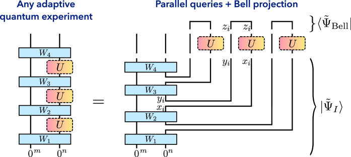
Figure 6: Visualization of the proof of Lemma 5, which relates the output state of any adaptive experiment involving $k$ queries to a unitary $U$ interleaved with arbitrary quantum circuits $W_{1},\ldots,W_{k+1}$, to the output of an experiment with only a single parallel query to $U^{\otimes k}$ (shown for $k=3$). The latter experiment applies $W_{1},\ldots,W_{k+1}$ to a series of Bell states (corresponding to the sums over $y_{i}$ in the text; shown for $i=2$) and swaps the output of each $W_{i}$ to an additional ancilla register (corresponding to the sums over $x_{i}$). After querying $U^{\otimes k}$, the additional ancilla registers are projected onto Bell states as shown (corresponding to the sums over $z_{i}$). By viewing each Bell state and Bell projector using tensor network notation, where each line denotes the entire Hilbert space of either a system or ancilla register, it becomes clear that the two experiments are equivalent. The normalization of the input state, $|\tilde{\Psi}_{I}\rangle$, and the Bell projector, $|\tilde{\Psi}_{\text{Bell}}\rangle$, are each $2^{nk}$. Hence, achieving a relative error in $U^{\otimes k}$ is crucial for capturing adaptive quantum experiments.

We define the following two unnormalized pure states,

$$\ket*{\widetilde{\Psi}_{U}} \coloneqq\sum_{\begin{subarray}{c}x_{1},\ldots,x_{k}\in\{0,1\}^{n}\\ y_{1},\ldots,y_{k}\in\{0,1\}^{n}\end{subarray}}W_{k+1}\cdot\prod_{i=1}^{k}((\outerproduct{y_{i}}{x_{i}}\otimes\mathbbm{1}_{A^{\prime}})\cdot W_{i})\ket{0^{n+m}}\otimes U^{\otimes k}\ket{x_{1},\ldots,x_{k}}\otimes\ket{y_{1},\ldots,y_{k}},$$ (B.9)

$$\ket*{\widetilde{\Psi}_{\mathrm{Bell}}} \coloneqq\sum_{\begin{subarray}{c}z_{1},\ldots,z_{k}\in\{0,1\}^{n}\end{subarray}}\ket{z_{1},\ldots,z_{k}}\otimes\ket{z_{1},\ldots,z_{k}}.$$ (B.10)

We can isolate the dependence on $U$ in the $(n+m+2kn)$-qubit unnormalized state $\ket*{\widetilde{\Psi}_{U}}$,

$$\ket*{\widetilde{\Psi}_{U}}=(\mathbbm{1}_{A,A^{\prime}}\otimes(U^{\otimes k}\otimes\mathbbm{1}_{A^{\otimes k}}))\ket*{\widetilde{\Psi}_{I}},$$ (B.11)

where $\mathbbm{1}_{A^{\otimes k}}$ acts as identity on $k$ copies of the $n$-qubit system. The output state $\ket*{\psi_{U}}$ can now be written as the partial inner product between the two unnormalized states,

$$\ket*{\psi_{U}}=(\mathbbm{1}_{A,A^{\prime}}\otimes\bra*{\widetilde{\Psi}_{\mathrm{Bell}}})\ket*{\widetilde{\Psi}_{U}}=(\mathbbm{1}_{A,A^{\prime}}\otimes\bra*{\widetilde{\Psi}_{\mathrm{Bell}}})(\mathbbm{1}_{A,A^{\prime}}\otimes(U^{\otimes k}\otimes\mathbbm{1}_{A^{\otimes k}}))\ket*{\widetilde{\Psi}_{I}}.$$ (B.12)

Recall that $\Phi_{\mathcal{E}}(A)\coloneqq\operatorname*{{\mathbb{E}}}_{U\sim\mathcal{E}}\left[U^{\otimes k}AU^{\dagger,\otimes k}\right]$. Using the above identity, we can write the output state $\outerproduct*{\psi_{U}}{\psi_{U}}$ averaged over random unitary $U$ sampled from the ensemble $\mathcal{E}$ as

$$\operatorname*{{\mathbb{E}}}_{U\sim\mathcal{E}}\outerproduct*{\psi_{U}}{\psi_{U}}=(I_{A,A^{\prime}}\otimes\bra*{\widetilde{\Psi}_{\mathrm{Bell}}})\cdot(\mathcal{I}_{A,A^{\prime}}\otimes\Phi_{\mathcal{E}}\otimes\mathcal{I}_{A^{\otimes k}})(\outerproduct*{\widetilde{\Psi}_{I}}{\widetilde{\Psi}_{I}})\cdot(I_{A,A^{\prime}}\otimes\ket*{\widetilde{\Psi}_{\mathrm{Bell}}}),$$ (B.13)

where $\mathcal{I}_{A,A^{\prime}}$ and $\mathcal{I}_{A^{\otimes k}}$ are the identity CPTP maps acting on register $A,A^{\prime}$ and the $k$-copy register $A^{\otimes k}$. Using the definition of relative error $(1-\varepsilon)\,\Phi_{H}\,\preceq\,\Phi_{\mathcal{E}}\,\preceq\,(1+\varepsilon)\,\Phi_{H}$, we have

$$(1-\varepsilon)\operatorname*{{\mathbb{E}}}_{U\sim\mathcal{E}_{H}}\outerproduct*{\psi_{U}}{\psi_{U}}\preceq\operatorname*{{\mathbb{E}}}_{U\sim\mathcal{E}}\outerproduct*{\psi_{U}}{\psi_{U}}\preceq(1+\varepsilon)\operatorname*{{\mathbb{E}}}_{U\sim\mathcal{E}_{H}}\outerproduct*{\psi_{U}}{\psi_{U}},$$ (B.14)

where for two positive-semidefinite matrices $A,B$, the relation $A\preceq B$ denotes that $B-A$ is positive semidefinite. Therefore, using the definition of $\norm{\cdot}_{1}$, we have

$$\begin{split}&\norm{\operatorname*{{\mathbb{E}}}_{U\sim\mathcal{E}}\outerproduct*{\psi_{U}}{\psi_{U}}-\operatorname*{{\mathbb{E}}}_{U\sim\mathcal{E}_{H}}\outerproduct*{\psi_{U}}{\psi_{U}}}_{1}\\ &\leq\max_{0\preceq M_{+},M_{-}\preceq I}\Tr\left(M_{+}\left[\operatorname*{{\mathbb{E}}}_{U\sim\mathcal{E}}\outerproduct*{\psi_{U}}{\psi_{U}}-\operatorname*{{\mathbb{E}}}_{U\sim\mathcal{E}_{H}}\outerproduct*{\psi_{U}}{\psi_{U}}\right]\right)\\ &\quad\quad\quad\quad\quad\,\,-\Tr\left(M_{-}\left[\operatorname*{{\mathbb{E}}}_{U\sim\mathcal{E}}\outerproduct*{\psi_{U}}{\psi_{U}}-\operatorname*{{\mathbb{E}}}_{U\sim\mathcal{E}_{H}}\outerproduct*{\psi_{U}}{\psi_{U}}\right]\right)\\ &\leq\max_{0\preceq M_{+},M_{-}\preceq I}\epsilon\Tr\left(M_{+}\operatorname*{{\mathbb{E}}}_{U\sim\mathcal{E}_{H}}\outerproduct*{\psi_{U}}{\psi_{U}}\right)+\epsilon\Tr\left(M_{-}\operatorname*{{\mathbb{E}}}_{U\sim\mathcal{E}_{H}}\outerproduct*{\psi_{U}}{\psi_{U}}\right)\\ &=2\varepsilon\norm{\operatorname*{{\mathbb{E}}}_{U\sim\mathcal{E}_{H}}\outerproduct*{\psi_{U}}{\psi_{U}}}_{1}=2\varepsilon.\end{split}$$ (B.15)

This concludes the proof of this lemma. ∎

B.2 A brief review of Haar random unitaries

In this appendix, we review several properties of Haar random unitaries. We let $\mathcal{H}$ be the Hilbert space of an $n$-qubit system, with Hilbert space dimension $D=2^{n}$, and $\mathcal{E}_{H}$ be the Haar-random unitary ensemble on $\mathcal{H}$. We begin by reviewing the expression for the Haar twirl, $\Phi_{H}$ [Eq. (B.2)], as a sum over permutation operators on $\mathcal{H}^{\otimes k}$. We then review the representation theory of the unitary and symmetric groups, and write the action of the twirl in the basis of irreducible representations.

B.2.1 Permutation operators and the Weingarten calculus

The $k$-fold Haar-random twirling channel can be expressed as the sum,

$$\Phi_{H}(A)\equiv\operatorname*{{\mathbb{E}}}_{U\sim\mathcal{E}_{H}}[U^{\otimes k}A\,(U^{\dagger})^{\otimes k}]=\sum_{\sigma,\tau\in S_{k}}\Tr(A\,\sigma^{-1})\,\text{Wg}(\sigma\tau^{-1};D)\,{\tau}.$$ (B.16)

Here, $\sigma,\tau\in S_{k}$ are permutations of $k$ elements. In a slight abuse of notation, we use the same symbols to denote the permutations’ representation on $\mathcal{H}^{\otimes k}$. The coefficients in the sum, $\text{Wg}(\,\cdot\,;D):S_{k}\to\mathbb{R}$, are known as the Weingarten function [168].

When $k\leq D$, the Weingarten function can be constructed as follows. Consider two permutations $\sigma,\tau\in S_{k}$ and define the function

$$G(\sigma\tau^{-1};D)\equiv\Tr(\sigma\tau^{-1})=D^{\#(\sigma\tau^{-1})}=D^{k-|\sigma\tau^{-1}|}$$ (B.17)

where $\#(\sigma\tau^{-1})$ is the number of cycles in $\sigma\tau^{-1}$, and $|\sigma\tau^{-1}|\equiv k-\#(\sigma\tau^{-1})$ defines a distance measure on the permutation group. The function $G(\cdot;D)$ can be viewed as a $k!\times k!$ symmetric Gram matrix, $\hat{G}(D)$, with matrix elements $G_{\sigma,\tau}(D)=G(\sigma\tau^{-1};D)$. We can similarly view the Weingarten function as a symmetric matrix, $\hat{\operatorname{Wg}}(D)$, with elements $\operatorname{Wg}_{\sigma,\tau}(D)=\operatorname{Wg}(\sigma\tau^{-1};D)$. For $k\leq D$, the Weingarten matrix is defined as the matrix inverse of $G_{\sigma,\tau}$. That is, we have

$$\sum_{\tau\in S^{k}}\operatorname{Wg}_{\sigma,\tau}(D)\,G_{\tau,\pi}(D)=\delta_{\sigma,\pi}\,.$$ (B.18)

While $G_{\sigma,\tau}(D)\geq 0$, the Weingarten matrix elements $\operatorname{Wg}_{\sigma,\tau}(D)$ may take negative values. In particular, we have $\operatorname{Wg}_{\sigma,\tau}(D)=(-1)^{|\sigma|}|\!\operatorname{Wg}_{\sigma,\tau}(D)|(-1)^{|\tau|}$.

A key property of the permutation operators is that they are approximately orthogonal when the Hilbert space dimension $D$ is large. This allows one to approximate $G_{\sigma,\tau}(D)\approx D^{k}\delta_{\sigma,\tau}$ and $\operatorname{Wg}_{\sigma,\tau}(D)\approx D^{-k}\delta_{\sigma,\tau}$ in many settings. This is captured by the following result from Ref. [55]:

Corollary of [55] (Approximate orthogonality).

Viewing $G_{\sigma,\tau}(D)$ as a $k!\times k!$ matrix $\hat{G}(D)$, its distance from the $k!\times k!$ identity matrix, $\hat{\mathbbm{1}}$, is bounded as

$$\left\lVert\frac{1}{D^{k}}\hat{G}(D)-\hat{\mathbbm{1}}\right\rVert_{\infty}\leq\frac{k^{2}}{D},\,\,\,\,\,\,\,\,\text{ for }k^{2}\leq D.$$ (B.19)

Viewing $\operatorname{Wg}_{\sigma,\tau}(D)$ and $|\!\operatorname{Wg}_{\sigma,\tau}(D)|$ similarly, we have

$$\left\lVert D^{k}\hat{\emph{W}}\emph{g}(D)-\hat{\mathbbm{1}}\right\rVert_{\infty}\leq\frac{\frac{k^{2}}{2D}}{1-\frac{k^{2}}{2D}}\,\,\,\,\,\text{and}\,\,\,\,\,\left\lVert D^{k}|\hat{\emph{W}}\emph{g}(D)|-\hat{\mathbbm{1}}\right\rVert_{\infty}\leq\frac{\frac{k^{2}}{2D}}{1-\frac{k^{2}}{2D}},\,\,\,\,\,\,\,\,\text{ for }k^{2}\leq D.$$ (B.20)

Proof.

Eq. (B.19) is shown in Lemma 1 of Ref. [55]. To derive Eq. (B.20), let us denote the maximum eigenvalue of $\hat{G}(D)$ as $\lambda_{\text{max}}$ and the minimum eigenvalue as $\lambda_{\text{min}}$. Since $\hat{\text{W}}\text{g}(D)$ is the inverse of $\hat{G}(D)$, its maximum and minimum eigenvalues are $\lambda_{\text{min}}^{-1}$ and $\lambda_{\text{max}}^{-1}$, respectively. These are the maximum and minimum eigenvalues of $|\hat{\text{W}}\text{g}(D)|$ as well, since $|\hat{\text{W}}\text{g}(D)|$ is related to $\hat{\text{W}}\text{g}(D)$ by a unitary rotation, $\hat{\text{W}}\text{g}(D)=\hat{P}|\hat{\text{W}}\text{g}(D)|\hat{P}$ with $P_{\sigma,\tau}=(-1)^{|\sigma|}\delta_{\sigma,\tau}$ [101]. From Lemma 1 of Ref. [55], we have $\lambda_{\text{max}}\leq e^{k^{2}/2D}$ and $\lambda_{\text{min}}\geq 1-\frac{k^{2}}{2D}$ when $k^{2}\leq D$, which immediately give Eq. (B.20). ∎

Before proceeding, we recall several properties of sums over $G(\cdot;D)$ and $\operatorname{Wg}(\cdot;D)$ that will be useful in our proofs. We have [101],

$$\sum_{\sigma}G(\sigma;D)=\frac{1}{\sum_{\sigma}\operatorname{Wg}(\sigma;D)}=\frac{(k+D-1)!}{D!}\leq D^{k}\left(1+\frac{k^{2}}{D}\right).$$ (B.21)

where the inequality holds for $k^{2}\leq D$. The sum over $G(\cdot;D)$ is the reciprocal of the sum over $\operatorname{Wg}(\cdot;D)$ because, in matrix notation, the sum corresponds to the eigenvalue of the constant vector, $v_{\sigma}=1/(\sqrt{k!})$ [101]. For the absolute value of the Weingarten function, we have [101]

$$\sum_{\tau\in S_{k}}|\text{\rm Wg}(\tau;D)|=\frac{(D-k)!}{D!}\leq\frac{1}{D^{k}}\left(1+\frac{k^{2}}{D}\right),$$ (B.22)

where the inequality holds for $k^{2}\leq D$.

B.2.2 The Schur-Weyl duality

Let us now introduce the representation theory of the symmetric group $S_{k}$ on the Hilbert space $\mathcal{H}^{\otimes k}$ [169, 170]. This material is needed only for our proof of Lemma 1 from the results of Ref. [50], which we provide at the end of this section.

The Schur-Weyl duality states that we can decompose $\mathcal{H}^{\otimes k}$ as a tensor sum,

$$\mathcal{H}^{\otimes k}=\bigoplus_{\lambda}\mathcal{Q}^{D}_{\lambda}\otimes\mathcal{P}_{\lambda}$$ (B.23)

where $\lambda$ labels the irreducible representations of the symmetric group $S_{k}$. Each $\lambda$ corresponds to a partition of $k$ and can be represented by a Young diagram. The space $\mathcal{P}_{\lambda}$ corresponds to an irreducible representation of $S_{k}$, with dimension given by the hook length formula,

$$\mathrm{dim}\mathcal{P}_{\lambda}=\text{dim}(\lambda)=\frac{k!}{\prod_{(i,j)\in\lambda}h_{i,j}},$$ (B.24)

where $h_{i,j}$ is the hook length of the box in the $i$-th row and $j$-th column of the Young diagram of $\lambda$. The space $\mathcal{Q}^{D}_{\lambda}$ labels the degeneracies of this representation, with a dimension

$$\mathrm{dim}\mathcal{Q}^{D}_{\lambda}=D_{\lambda}[k]=\frac{\text{dim}(\lambda)D^{\uparrow\lambda}}{k!}$$ (B.25)

that depends on both $\lambda$ and the total dimension $D$. Here, $D^{\uparrow\lambda}$ denotes the rising factorial of the partition $\lambda$; see Ref. [170]. Observing the definition of $D^{\uparrow\lambda}$ in Ref. [170], we can upper bound

$$D^{\uparrow\lambda}\leq D^{k}\left(1+\frac{k^{2}}{2D}\right).$$ (B.26)

The space $\mathcal{Q}^{D}_{\lambda}$ also corresponds to an irreducible representation of $\mathrm{SU}(D)$. Using the three equations characterizing the dimensions given above, we have

$$\max_{\lambda}\left[\frac{D^{k}\cdot\mathrm{dim}\mathcal{Q}_{\lambda}^{2^{n}}}{\mathrm{dim}\mathcal{P}_{\lambda}}\right]\leq\frac{D^{2k}}{k!}\left(1+\frac{k^{2}}{2D}\right).$$ (B.27)

By following the proof of Lemma 30 of [50] without lower bounding $\frac{\mathrm{dim}\mathcal{P}_{\lambda}}{D^{k}\cdot\mathrm{dim}\mathcal{Q}_{\lambda}^{2^{n}}}$ using the lossy inequality $\binom{N+t-1}{t}\leq N^{t}$, we obtain the following lemma.

Lemma 6 (Lemma 30 of [50] without bounding the eigenvalues).

A random unitary ensemble $\mathcal{E}$ acting on an $n$-qubit Hilbert space $\mathcal{H}$ forms an $\varepsilon$-approximate unitary $k$-design with error

$$\varepsilon=\max_{\lambda}\left[\frac{2^{nk}\cdot\mathrm{dim}\mathcal{Q}_{\lambda}^{2^{n}}}{\mathrm{dim}\mathcal{P}_{\lambda}}\right]\cdot\big{\lVert}\,[(\Phi_{\mathcal{E}}-\Phi_{H})\otimes\mathbbm{1}](P^{\mathrm{EPR}})\,\big{\rVert}_{\infty},$$ (B.28)

where $P^{\mathrm{EPR}}$ is the projector onto the EPR state on $\mathcal{H}^{\otimes k}\otimes\mathcal{H}^{\otimes k}$.

Lemma 1 follows from this lemma after plugging Eq. (B.27) into Eq. (B.28).

B.3 Proof of Theorem 1: Gluing small random unitary designs

This appendix provides the details for proving Theorem 1. We refer the readers to Section 4 in the main text for an overview of the proof.

B.3.1 Residual of the Haar twirl

To simplify our analysis of the spectral norm in Lemma 1, we first prove the following lemma. We call $\Phi^{r}_{\mathcal{E}}$ the residual of the Haar twirl.

Lemma 7 (Residual of the Haar twirl).

Consider a unitary ensemble $\mathcal{E}$, and suppose we can decompose $\Phi_{\mathcal{E}}=\Phi_{\mathcal{E}}^{i}+\Phi_{\mathcal{E}}^{r}$, where $\Phi_{\mathcal{E}}^{i}$ is invariant under the Haar twirl, i.e. $\Phi_{\mathcal{E}}^{i}\circ\Phi_{H}=\Phi_{\mathcal{E}}^{i}$. Then

$$\norm{[(\Phi_{\mathcal{E}}-\Phi_{H})\otimes\mathbbm{1}](P^{\mathrm{EPR}})}_{\infty}\leq 2\norm{[\Phi_{\mathcal{E}}^{r}\otimes\mathbbm{1}](P^{\mathrm{EPR}})}_{\infty}.$$ (B.29)

Proof.

We know that $\Phi_{\mathcal{E}}\circ\Phi_{H}=\Phi_{H}$ for any unitary ensemble $\mathcal{E}$. Applied to $\Phi_{\mathcal{E}}=\Phi_{\mathcal{E}}^{i}+\Phi_{\mathcal{E}}^{r}$, we have $\Phi_{\mathcal{E}}^{i}=\Phi_{H}-\Phi_{\mathcal{E}}^{r}\circ\Phi_{H}$, and thus $\Phi_{\mathcal{E}}-\Phi_{H}=\Phi_{\mathcal{E}}^{r}-\Phi_{\mathcal{E}}^{r}\circ\Phi_{H}$. We now have $[(\Phi_{\mathcal{E}}-\Phi_{H})\otimes\mathbbm{1}](P^{\mathrm{EPR}})=[\Phi_{\mathcal{E}}^{r}\otimes\mathbbm{1}](P^{\mathrm{EPR}})-[\Phi_{H}\otimes\mathbbm{1}]\circ[\Phi_{\mathcal{E}}^{r}\otimes\mathbbm{1}](P^{\mathrm{EPR}})$. By the triangle inequality and the fact that $\norm{[\Phi_{H}\otimes\mathbbm{1}](A)}_{\infty}\leq\norm{A}_{\infty}$, we obtain the desired claim. ∎

B.3.2 Gluing two random unitaries

We now prove Lemma 2 of the main text, which allows us to “glue” together approximate designs on local patches of qubits to form larger approximate designs. We first re-state the lemma with an error bound that yields tighter constants for the applications.

Lemma 8 (Gluing two random unitaries, formal).

Let $A$, $B$, $C$ be three disjoint subsystems. Consider a random unitary given by $V_{ABC}=U_{AB}U_{BC}$, where $U_{AB}$ and $U_{BC}$ are drawn from $\varepsilon_{AB}$ and $\varepsilon_{BC}$-approximate unitary $k$-designs, respectively. Then $V_{ABC}$ is an $\varepsilon$-approximate unitary $k$-design for

$$1+\varepsilon=(1+\varepsilon_{AB})(1+\varepsilon_{BC})\left(1+2\left(\frac{k^{2}}{D_{B}}+\frac{k^{2}}{D_{BC}}+\frac{k^{4}}{D_{B}D_{BC}}+\frac{\frac{k^{2}}{2D_{BC}}}{1-\frac{k^{2}}{2D_{BC}}}\right)\left(1+\frac{k^{2}}{D_{AB}}\right)\right),$$ (B.30)

as long as $k^{2}\leq D_{B}$, where $D_{\alpha}=2^{|\alpha|}$ is the Hilbert space dimension of subsystem $\alpha$.

Proof.

Let us first consider the case when $U_{AB}$ and $U_{BC}$ are Haar-random, and let $\mathcal{E}^{*}$ denote the corresponding ensemble of $V_{ABC}$. Let $\Phi_{\mathcal{E}^{*}}$ denote the $k$-wise twirl over $V_{ABC}$. From Lemma 1 and Lemma 7, the relative error of $\mathcal{E}^{*}$ is bounded by the spectral norm when the residual channel, $\Phi^{r}_{\mathcal{E}^{*}}$, is applied to the EPR state. From Eq. (B.16), we can write $\Phi_{\mathcal{E}}$ as

$$\Phi_{\mathcal{E}^{*}}(\cdot)=\sum_{\sigma,\tau,\tilde{\sigma},\tilde{\tau}}\Tr_{ABC}\left((\cdot)(\tilde{\sigma}_{A}\sigma_{BC})^{-1}\right)\,\text{Wg}_{BC}(\sigma\tau^{-1})\,\Tr_{B}(\tau_{B}\tilde{\sigma}_{B}^{-1})\,\text{Wg}_{AB}(\tilde{\sigma}\tilde{\tau}^{-1})\,\tilde{\tau}_{AB}\tau_{C}$$ (B.31)

where the subscripts denote which subsystem the permutations act upon. To define the residual channel, we note that the subset of terms in Eq. (B.31) with $\tau=\tilde{\tau}$ are invariant under the Haar twirl. Thus, we can define $\Phi^{r}_{\mathcal{E}^{*}}$ as the sum of the remaining terms with $\tau\neq\tilde{\tau}$. We have

$$[\Phi^{r}_{\mathcal{E}^{*}}\otimes\mathbbm{1}](P^{EPR})=D^{-k}\sum_{\sigma,\tilde{\sigma},\tau\neq\tilde{\tau}}\text{Wg}_{BC}(\sigma\tau^{-1})\,\Tr_{B}(\tau_{B}\tilde{\sigma}_{B}^{-1})\,\text{Wg}_{AB}(\tilde{\sigma}\tilde{\tau}^{-1})\,[\tilde{\tau}_{AB}\tau_{C}\otimes\tilde{\sigma}_{A}\sigma_{BC}],$$ (B.32)

where $D=2^{|A|+|B|+|C|}$ is the total Hilbert space dimension, and we use that $\Tr_{1}([A\otimes\mathbbm{1}]P^{\mathrm{EPR}})=D^{-k}[\mathbbm{1}\otimes A^{T}]$ for any operator $A$ on $\mathcal{H}^{\otimes k}$, where the trace is over the first copy of $\mathcal{H}^{\otimes k}$.

We can bound the spectral norm via the triangle inequality,

$$\begin{split}\lVert[\Phi^{r}_{\mathcal{E}^{*}}\otimes\mathbbm{1}](P^{EPR})\rVert_{\infty}&\leq D^{-k}\sum_{\sigma,\tilde{\sigma},\tau\neq\tilde{\tau}}|\text{Wg}_{BC}(\sigma\tau^{-1})|\,\Tr_{B}(\tau_{B}\tilde{\sigma}_{B}^{-1})\,|\text{Wg}_{AB}(\tilde{\sigma}\tilde{\tau}^{-1})|\\ \end{split}$$ (B.33)

We decompose the remaining sum as $\sum_{\tau\neq\tilde{\tau}}=\sum_{\tau,\tilde{\tau}}-\sum_{\tau=\tilde{\tau}}$. The first term is

$$\begin{split}\sum_{\sigma,\tilde{\sigma},\tau,\tilde{\tau}}|\text{Wg}_{BC}(\sigma\tau^{-1})|\,\Tr_{B}(\tau_{B}\tilde{\sigma}_{B}^{-1})\,|\text{Wg}_{AB}(\tilde{\sigma}\tilde{\tau}^{-1})|&=k!\frac{(D_{AB}-k)!}{D_{AB}!}\frac{(k+D_{B}-1)!}{D_{B}!}\frac{(D_{BC}-k)!}{D_{BC}!}\\ &\leq\frac{k!}{D_{C}^{k}}\frac{(D_{AB}-k)!}{D_{AB}!}\left(1+\frac{k^{2}}{D_{B}}\right)\left(1+\frac{k^{2}}{D_{BC}}\right),\end{split}$$ (B.34)

where we use Eq. (B.22) to compute the sums over $\sigma,\tilde{\tau}$ and Eq. (B.21) to compute the sum over $\tau$. The second term is

$$\sum_{\sigma,\tilde{\sigma},\tilde{\tau}}|\text{Wg}_{BC}(\sigma\tilde{\tau}^{-1})|\,\Tr_{B}(\tilde{\tau}_{B}\tilde{\sigma}_{B}^{-1})\,|\text{Wg}_{AB}(\tilde{\sigma}\tilde{\tau}^{-1})|\geq\frac{k!}{D_{C}^{k}}\frac{(D_{AB}-k)!}{D_{AB}!}\left(1-\frac{\frac{k^{2}}{2D_{BC}}}{1-\frac{k^{2}}{2D_{BC}}}\right),$$ (B.35)

where we again use Eq. (B.22) to compute the sum over $\sigma$. To bound the remaining sum over $\tilde{\sigma}$ and $\tilde{\tau}$, we write $|\text{Wg}_{BC}(\tilde{\sigma}\tilde{\tau}^{-1})|=D_{BC}^{-k}(\delta_{\tilde{\sigma},\tilde{\tau}}+\delta W_{\tilde{\sigma},\tilde{\tau}})$, where $\lVert\delta W\rVert_{\infty}\leq f/(1-f)$, $f=k^{2}/2D_{BC}$ by Eq. (B.20). We then apply $\sum_{\tilde{\sigma},\tilde{\tau}}G_{\tilde{\tau},\tilde{\sigma}}(D_{B})\delta W_{\tilde{\sigma},\tilde{\tau}}\leq\lVert\hat{G}(D_{B})\rVert_{1}\lVert\delta W\rVert_{\infty}$, where we recall $G_{\tilde{\tau},\tilde{\sigma}}(D_{B})=\Tr_{B}(\tilde{\tau}_{B}\tilde{\sigma}_{B}^{-1})$ and we have $\lVert\hat{G}(D_{B})\rVert_{1}=\sum_{\tilde{\sigma}}G_{\tilde{\sigma},\tilde{\sigma}}=k!D_{B}^{k}$ since $\hat{G}(D_{B})$ is a positive matrix. Together with Eq. (B.33), we have

$$\begin{split}\lVert[\Phi^{r}_{\mathcal{E}^{*}}\otimes\mathbbm{1}](P^{EPR})\rVert_{\infty}&\leq\frac{k!}{D^{k}D_{C}^{k}}\frac{(D_{AB}-k)!}{D_{AB}!}\left(\frac{k^{2}}{D_{B}}+\frac{k^{2}}{D_{BC}}+\frac{k^{4}}{D_{B}D_{BC}}+\frac{\frac{k^{2}}{2D_{BC}}}{1-\frac{k^{2}}{2D_{BC}}}\right)\\ &\leq\frac{k!}{D^{2k}}\left(1+\frac{k^{2}}{D_{AB}}\right)\left(\frac{k^{2}}{D_{B}}+\frac{k^{2}}{D_{BC}}+\frac{k^{4}}{D_{B}D_{BC}}+\frac{\frac{k^{2}}{2D_{BC}}}{1-\frac{k^{2}}{2D_{BC}}}\right)\\ \end{split}$$ (B.36)

Applying Lemmas 1 and 7 shows that $\mathcal{E}^{*}$ is a design with error given by the last term in Eq. (B.30).

We can now return to the case when $U_{AB}$, $U_{BC}$ are drawn from approximate designs. Let $\mathcal{E}$ denote the corresponding ensemble of $V_{ABC}$. From the definition of approximate designs, we have

$$(1-\varepsilon_{AB})(1-\varepsilon_{BC})\Phi_{\mathcal{E}^{*}}\preceq\Phi_{\mathcal{E}}\preceq(1+\varepsilon_{AB})(1+\varepsilon_{BC})\Phi_{\mathcal{E}^{*}}.$$ (B.37)

Combined with Eq. (B.36), $\mathcal{E}$ forms an $\varepsilon$-approximate unitary $k$-design with $\varepsilon$ as in Eq. (B.30). ∎

B.3.3 Completing the proof of Theorem 1

Proof of Theorem 1.

We apply Lemma 2 (Lemma 8) patch-by-patch as described in Section 4 in the main text and Fig. 5. Recall that $m$ is the number of local patches in the $n$-qubit system, and the number of small random unitaries is equal to $m-1$. After all $m-2$ applications of Lemma 8, we find that the two-layer brickwork ensemble forms an approximate unitary $k$-design with error

$$\begin{split}(1+\varepsilon/n)^{m-1}\left(1+f(k,q)\right)^{m-2}-1&\leq e^{(m-1)\varepsilon/n+(m-2)f(k,q)}-1\\ &\leq\frac{1}{\log(2)}\left((m-1)\varepsilon/n+(m-2)f(k,q)\right),\end{split}$$ (B.38)

where we use the inequality $e^{x}-1\leq x/\log(2)$ for $x\leq\log(2)$, and we abbreviate,

$$f(k,q)=2\left(\frac{k^{2}}{q}+\frac{k^{2}}{q^{2}}+\frac{k^{4}}{q^{3}}+\frac{k^{2}/2q^{2}}{1-k^{2}/2q^{2}}\right)\left(1+\frac{k^{2}}{q^{2}}\right).$$ (B.39)

To establish the theorem, we will show that the error, Eq. (B.38), is less than $\varepsilon$.

We take $k\geq 2$ and $n\geq 3\xi$ since otherwise the theorem holds trivially. Combined with the assumptions $q\geq nk^{2}/\varepsilon$ and $\varepsilon\leq 1$, these imply that $\xi\geq 7$, i.e. $q\geq 128$. Observing the first term in Eq. (B.38), we have

$$\frac{(m-1)\varepsilon}{n\log(2)}\leq\frac{\varepsilon}{7\log(2)},$$ (B.40)

since $m\leq n/\xi\leq n/7$. Meanwhile, applying $q\geq nk^{2}/\varepsilon$ to the second term in Eq. (B.38), we have

$$\begin{split}e(m-2)f(k,q)&\leq\frac{n}{7\log(2)}\cdot 2\left(\frac{\varepsilon}{n}+\frac{\varepsilon}{nq}+\frac{\varepsilon^{2}}{n^{2}q}+\frac{\frac{\varepsilon}{2nq}}{1-\frac{\varepsilon}{2nq}}\right)\left(1+\frac{\varepsilon}{nq}\right)\leq\varepsilon\cdot\frac{3}{7\log(2)}.\end{split}$$ (B.41)

Taking the sum of the two terms shows that the error is less than $\varepsilon\cdot 4/7\log(2)\leq\varepsilon$ as desired. ∎

B.4 Proof of Corollary 1: Low-depth random unitary designs

Our construction in Theorem 1 enables one to exponentially improve the $n$ dependence of the depth of random unitary designs compared to existing constructions. In this appendix, we present several examples of low-depth random unitary designs that can be realized by inserting existing constructions of unitary designs into the small random unitaries in our own construction.

Proof of Corollary 1: We begin with the proof of Corollary 1. To obtain the stated depth for 1D circuits, we replace each small random unitary in Theorem 1 with a 1D local random circuit on $2\xi$ qubits. From Ref. [62], such circuits form $\frac{\varepsilon}{n}$-approximate $k$-designs in depth $\mathcal{O}(\log^{7}(k)(k\xi+\log(n/\varepsilon)))$, for $k\leq c2^{2\xi/5}$, $c=\mathcal{O}(1)$. Setting $\xi=\log_{2}(nk^{2}/\varepsilon)$, we obtain an $\varepsilon$-approximate $k$-design in depth $d=\mathcal{O}(\log(nk/\varepsilon)\cdot k\log^{7}(k))=\mathcal{O}(\log(n/\varepsilon)\cdot k\,\text{poly}\log(k))$, as claimed.

In the specific case of $k=2,3$, we can take the small random unitaries to be random Clifford unitaries, since the Clifford unitaries form exact 2- and 3-designs [90, 91]. We can then exploit the fact that, for circuits with all-to-all connected (i.e. geometrically non-local) two-qubit gates, any Clifford circuit on $2\xi$ qubits can be implemented in depth $\mathcal{O}(\log\xi)$ using non-local CNOT gates and $(2\xi)^{2}$ ancilla qubits [92, 93]. Setting $\xi=\log_{2}(9n/\varepsilon)$, we obtain $\varepsilon$-approximate 2- and 3-designs in depth $\mathcal{O}(\log\log(n/\varepsilon))$ using $\mathcal{O}(n\log(n/\varepsilon))$ ancilla qubits. This proves the second claim of Corollary 1.

1D log-depth Clifford circuits: Ref. [90] proved that Clifford circuits form exact $3$-designs and Refs. [171, 172, 173] showed that all Clifford circuits over $2\xi$ qubits can be implemented in 1D with depth $\mathcal{O}(\xi)$. Hence, using our construction, one can create $\varepsilon$-approximate unitary $3$-designs over $n$ qubits using 1D Clifford circuits of depth

$$d=\mathcal{O}\left(\log(n/\varepsilon)\right).$$ (B.42)

This is particularly useful in classical shadow tomography [19].

Low-depth unitary designs with explicit constants: Ref. [61] constructs $\frac{\varepsilon}{n}$-approximate unitary $k$-designs on $2\xi$ qubits with depth $\mathcal{O}(k^{2}\xi^{2}+k\xi\log(n/\varepsilon))$ for 1D circuits and $\mathcal{O}(k^{2}\xi\log(\xi)+k\log(\xi)\log(n/\varepsilon))$ for general circuits. While the $k$-dependence is not optimal as in Ref. [62], the design depth in Ref. [61] comes with very small constants, which may make the bound more practical. More concretely, plugging the design depth of $(4\log(8)(2\xi)k^{2}+4k\log(n/\varepsilon))\cdot 2\log_{2}(2\xi)$ for general circuits [61] into Theorem 1, we obtain $\varepsilon$-approximate unitary $k$-designs over $n$ qubits with depth

$$d =8\log(2\log(nk^{2}/\varepsilon))(2\log(8)k^{2}\log(nk^{2}/\varepsilon)+k\log(n/\varepsilon)),$$ (B.43)

which is nearly quadratic in $k$ and nearly linear in $\log(n)$.

B.5 Proof of Proposition 1: Lower bounds for unitary designs

We now provide our proof of Proposition 1, as described in the main text.

Proof.

We consider the output distribution when a random unitary $U$ from the ensemble of interest is applied to the zero state, and the resulting state is measured in a random product basis. Let us denote the random basis states as $\{v\ket{x}\}$, where $v$ is a tensor product of single-qubit unitaries and $x\in\{0,1\}^{n}$. Each outcome $x$ occurs with probability

$$p_{U,v}(x)=\left|\bra{x}v^{\dagger}U\ket{0^{n}}\right|^{2}.$$ (B.44)

We consider the expectation value of the collision probability over both the random unitary and the random basis, multiplied by $2^{n}$ for convenience,

$$Z_{\mathcal{E}}=2^{n}\operatorname*{{\mathbb{E}}}_{U\sim\mathcal{E},v}\left[\sum_{x}p_{U,v}(x)^{2}\right].$$ (B.45)

For a Haar-random unitary, one finds $Z_{H}=2$ [22, 123]. Hence, for $\mathcal{E}$ to form a 2-design with relative error $\varepsilon$, we require $Z_{\mathcal{E}}\leq 2(1+\varepsilon)$.

We can further analyze the collision probability by performing the average over the random basis $v$. Applying a standard formula for the twirl over a tensor product of single-qubit 2-designs [17], we have

$$Z_{\mathcal{E}}=2^{n}\operatorname*{{\mathbb{E}}}_{U\sim\mathcal{E}}\left[\,\sum_{\ell=0}^{n}3^{-\ell}\tr\big(U\outerproduct{0^{n}}{0^{n}}U^{\dagger}\cdot\mathcal{P}_{\ell}\big{\{}U\outerproduct{0^{n}}{0^{n}}U^{\dagger}\big{\}}\big{missing})\right],$$ (B.46)

where $\mathcal{P}_{\ell}$ is a super-operator that projects onto Pauli operators with weight $\ell$. The contribution of each Pauli operator is damped exponentially in its weight, by $3^{-\ell}$, which is equal to the probability that the Pauli commutes with the random measurement basis.

To proceed, let us decompose the initial state $\outerproduct{0^{n}}{0^{n}}$ as a sum of three operators,

$$\outerproduct{0^{n}}{0^{n}}=\frac{1}{2^{n}}\mathbbm{1}+\rho_{1}+\rho_{>}.$$ (B.47)

The first operator is the identity component of the state, which has weight zero. The second operator is defined to contain all stabilizers of the state with weight one, $\rho_{1}=\frac{1}{2^{n}}\sum_{i}Z_{i}$. The third operator, $\rho_{>}$, contains all of the remaining stabilizers, which have weight greater than one. The three operators are orthogonal by definition.

After $U$ is applied, the first operator is unchanged and the second operator is evolved into an operator with weight at most $L$, where $L$ is the number of qubits in the light-cone of the unitary $U$. In 1D circuits, we have $L=2d$ where $d$ is the depth of $U$. In all-to-all circuits, we have $L=2^{d}$.

To lower bound the collision probability in terms of the circuit depth $d$, let us consider the total support of $U\outerproduct{0^{n}}{0^{n}}U^{\dagger}$ on weights between 1 and $L$,

$$P_{L}\equiv\sum_{\ell=1}^{L}\tr(U\outerproduct{0^{n}}{0^{n}}U^{\dagger}\cdot\mathcal{P}_{\ell}\{U\outerproduct{0^{n}}{0^{n}}U^{\dagger}\}).$$ (B.48)

The restriction to $\ell\geq 1$ eliminates the first operator in Eq. (B.47). Since the second and third operators are orthogonal before we apply $U$, they are also orthogonal after we apply $U$. Moreover, they remain orthogonal even after projecting to weights $\ell\leq L$, since $\rho_{1}$ only has support on such weights. Thus, we have

$$P_{L}=\tr(\rho_{1}^{2})+\sum_{\ell=0}^{L}\tr(U\rho_{>}U^{\dagger}\cdot\mathcal{P}_{\ell}\{U\rho_{>}U^{\dagger}\})\geq\frac{n}{2^{n}}.$$ (B.49)

The lower bound follows because the second term is non-negative and the first term is equal to $n/2^{n}$. This in turn lower bounds the expected collision probability,

$$\begin{split}Z_{\mathcal{E}}&\geq 1+2^{n}3^{-L}P_{L}\geq 1+\frac{n}{3^{L}}.\end{split}$$ (B.50)

For $\mathcal{E}$ to form an $\varepsilon$-approximate 2-design, we require $n/3^{L}\leq 1+2\varepsilon$. This requires depth

$$d\geq\frac{1}{2}\log_{3}\left(\frac{n}{1+2\varepsilon}\right)$$ (B.51)

in 1D circuits, and depth

$$d\geq\log_{2}\left(\log_{3}\left(\frac{n}{1+2\varepsilon}\right)\right),$$ (B.52)

in general all-to-all circuit architectures. ∎

Appendix C Pseudorandom unitaries

In this appendix, we present the definition of pseudorandom unitaries, a simple construction for pseudorandom unitaries, a proof of our main theorem (Theorem 2) for gluing small pseudorandom unitaries, and a proof of Corollary 2 for constructing low-depth pseudorandom unitaries.

C.1 Definition of pseudorandom unitaries

We begin with the formal definition of pseudorandom unitaries with security against $t(n)$-time adversaries, based on the definitions proposed in [47, 60, 59].

Definition 2 (Pseudorandom unitaries).

Let $n\in\mathbb{N}$ be the number of qubits. An infinite sequence $\{\mathcal{U}_{n}\}_{n\in\mathbb{N}}$ of $n$-qubit unitary ensembles $\mathcal{U}_{n}=\{U_{\mathsf{key}}\}_{\mathsf{key}\in\mathcal{K}_{n}}$ for the key space $\mathcal{K}_{n}$ is a pseudorandom unitary secure against any $t(n)$-time adversary if it satisfies the following.

• Efficient computation: There exists a $\mathrm{poly}(n)$-time quantum algorithm that implements the $n$-qubit unitary $U_{\mathsf{key}}$ for all $\mathsf{key}\in\mathcal{K}_{n}$.

• Indistinguishability from Haar: Any quantum algorithm $\mathcal{A}^{U}(1^{n})$ that runs in time $\leq t(n)$, queries an $n$-qubit unitary $U$ for any number of times, and outputs $\{0,1\}$ satisfies

  $$\left|\Pr_{\mathsf{key}\sim\mathcal{K}_{n}}\left[\mathcal{A}^{U_{\mathsf{key}}}(1^{n})=1\right]-\Pr_{U\sim\mathcal{E}_{H}}\left[\mathcal{A}^{U}(1^{n})=1\right]\right|\leq\mathrm{negl}(n),$$ (C.1)

  where $\mathcal{E}_{H}$ is the Haar-random unitary ensemble and $\mathrm{negl}(n)$ is the negligible function, i.e., a function that is asymptotically smaller than any inverse-polynomial function $1/\mathrm{poly}(n)$.

A $t(n)$-time algorithm $\mathcal{A}^{U}(1^{n})$ is referred to as a $t(n)$-time adversary. The difference between the probability under $\mathcal{U}_{n}$ and Haar ensemble is referred to as the advantage of $\mathcal{A}^{U}(1^{n})$.

When the pseudorandom unitary is secure against a $\operatorname{poly}(n_{\mathrm{big}})$-time adversary, where $n_{\mathrm{big}}$ is a function of $n$ that grows faster than $n$, $\mathrm{negl}(n)$ can be strengthened to $\mathrm{negl}(n_{\mathrm{big}})$.

Fact 1 (Strengthening the negligible function).

Let $n_{\mathrm{big}}$ be a function of $n$ such that $n_{\mathrm{big}}=\Omega(n)$. For any $n$-qubit pseudorandom unitary secure against $\operatorname{poly}(n_{\mathrm{big}})$-time adversary, we can show that any quantum algorithm $\mathcal{A}^{U}(1^{n})$ that runs in $\operatorname{poly}(n_{\mathrm{big}})$ time, queries an $n$-qubit unitary $U$ for any number of times, and outputs $\{0,1\}$ must satisfy

$$\left|\Pr_{\mathsf{key}\sim\mathcal{K}_{n}}\left[\mathcal{A}^{U_{\mathsf{key}}}(1^{n})=1\right]-\Pr_{U\sim\mathcal{E}_{H}}\left[\mathcal{A}^{U}(1^{n})=1\right]\right|\leq\mathrm{negl}(n_{\mathrm{big}}),$$ (C.2)

where $\mathrm{negl}(n_{\mathrm{big}})$ is a function asymptotically smaller than any inverse-polynomial function in $n_{\mathrm{big}}$.

Proof.

If the advantage of a $\operatorname{poly}(n_{\mathrm{big}})$-time algorithm $\mathcal{A}$ is at least $1/\operatorname{poly}(n_{\mathrm{big}})$, then one could construct another $\operatorname{poly}(n_{\mathrm{big}})$-time algorithm that repeats $\mathcal{A}$ for $\operatorname{poly}(n_{\mathrm{big}})$ many times and votes on the outputs of the repetitions to achieve a constant advantage. This contradicts with the condition Eq. (C.1). Hence, the advantage of any $\operatorname{poly}(n_{\mathrm{big}})$-time algorithm $\mathcal{A}$ is negligible in $n_{\mathrm{big}}$. ∎

C.2 The $PFC$ construction for pseudorandom unitaries

A proposed construction of pseudorandom unitaries [60] is the $PFC$ ensemble, where $C$ is a random Clifford circuit over $n$ qubits, $F$ is a quantum-secure pseudorandom function (PRF) over $n$ bits given by a random real diagonal unitary with diagonal elements $\pm 1$ [95], and $P$ is a quantum-secure pseudorandom permutation (PRP) [96] over $n$ bits. Assuming no subexponential-time quantum algorithms can solve the Learning With Errors (LWE) problem [94], existing works [96, 95] have constructed quantum-secure pseudorandom functions $F$ and quantum-secure pseudorandom permutations $P$ that are secure against any subexponential-time quantum algorithms.

Fact 2 (Circuit depth of $P$ and $F$; [96, 95]).

The $n$-qubit unitaries $P$ and $F$ can both be implemented using quantum circuit depth $\mathrm{poly}(n)$ in 1D circuits and circuit depth $\mathrm{poly}\log(n)$ in all-to-all-connected circuits. The number of ancilla qubits scales as $\mathrm{poly}(n)$.

Fact 3 (Circuit depth of Clifford $C$; [92, 93]).

Any $n$-qubit Clifford circuit $C$ can be implemented in $\mathcal{O}(n)$ depth in 1D circuits without using any ancilla qubits and $\mathcal{O}(\log n)$ depth in all-to-all-connected circuits using $\mathcal{O}(n^{2})$ ancilla qubits.

Using the two facts above, we arrive at the following fact.

Fact 4 (Circuit depth of $PFC$).

Any $n$-qubit unitary $U=PFC$ can be implemented using quantum circuit depth $\mathrm{poly}(n)$ in 1D circuits and circuit depth $\mathrm{poly}\log(n)$ in all-to-all-connected circuits. The number of ancilla qubits scales as $\mathrm{poly}(n)$.

While establishing indistinguishability between the $PFC$ ensemble and the Haar ensemble under the hardness assumption of LWE remains a conjecture in Ref. [60], a forthcoming work [65] has resolved this conjecture using a surprisingly simple proof. The formal statement [65] is given below.

Theorem 3 ($PFC$ is a pseudorandom unitary; [65]).

Let $n$ be the number of qubits. Consider any subexponential function $t(n)=\exp(o(n))$. Given a quantum-secure pseudorandom function $F$ over $n$ bits secure against $t(n)$-time adversary, a quantum-secure pseudorandom permutation $P$ over $n$ bits secure against $t(n)$-time adversary, and a random $n$-qubit Clifford circuit $C$. The $n$-qubit random unitary ensemble $U=PFC$ is a pseudorandom unitary secure against any $t(n)$-time adversary.

As a result, under the cryptographic assumption that there are no subexponential-time quantum algorithms for solving LWE, one can show that the random unitary ensemble $PFC$ is a pseudorandom unitary secure against any subexponential-time quantum algorithms, i.e., $t(n)=\exp(o(n))$ in Def. 2.

C.3 Proof of Theorem 2: Gluing small pseudorandom unitaries

We re-state and prove Theorem 2, which shows that we can use the two-layer brickwork ensemble to glue small pseudorandom unitaries over $\omega(\log n)$ local patches of qubits into a pseudorandom unitary on $n$ qubits.

Theorem 4 (Gluing small pseudorandom unitaries).

Let $n$ be the number of qubits in the whole system and $\xi=\omega(\log n)$ be the number of qubits in each local patch. Suppose each small random unitary in the two-layer brickwork ensemble $\mathcal{E}$ is a $2\xi$-qubit pseudorandom unitary secure against $\operatorname{poly}(n)$-time adversaries. Then $\mathcal{E}$ is an $n$-qubit pseudorandom unitary secure against $\operatorname{poly}(n)$-time adversaries.

Proof.

Let us consider a two-layer brickwork ensemble $\mathcal{E}^{*}$ over $n$ qubits, where each of the small random unitaries over $2\xi$ qubits are Haar-random. We will prove the following two claims: (1) any $\mathrm{poly}(n)$-time quantum algorithm cannot distinguish between $\mathcal{E}$ and $\mathcal{E}^{*}$, (2) any $\mathrm{poly}(n)$-time quantum algorithm cannot distinguish between $\mathcal{E}^{*}$ and Haar-random ensemble. Hence, any $\mathrm{poly}(n)$-time quantum algorithm cannot distinguish between $\mathcal{E}$ and Haar-random ensemble.

Proving Claim (1). We use a hybrid argument to establish the claim. Recall that $m-1$ is the number of small random unitaries in the two-layer brickwork. We consider a sequence of $m$ ensembles $\mathcal{E}_{0},\ldots,\mathcal{E}_{m-1}$, where $\mathcal{E}_{j}$ corresponds to having the first $j$ small random unitaries sampled from a $2\xi$-qubit pseudorandom unitary secure against $\operatorname{poly}(n)$-time adversaries, and the rest of the $m-1-j$ small random unitaries sampled from the Haar ensemble. By definition, we have $\mathcal{E}_{0}=\mathcal{E}$ and $\mathcal{E}_{m-1}=\mathcal{E}^{*}$. The advantage of any $\mathrm{poly}(n)$-time quantum algorithm $\mathcal{A}$ to distinguish between $\mathcal{E}_{j-1}$ and $\mathcal{E}_{j}$ can be bounded above using a proof of contradiction.

Using Fact 1 with $n,n_{\mathrm{big}}\leftarrow 2\xi,n$, for any $2\xi$-qubit pseudorandom unitary ensemble $\mathcal{V}$ secure against $\operatorname{poly}(n)$-time adversaries, we can bound the advantage of any algorithm $\mathcal{A}^{V}$ that runs in $\operatorname{poly}(n)$ time, queries a $2\xi$-qubit unitary $V\sim\mathcal{V}$ for any number of times, and outputs $\{0,1\}$, as follows,

$$\left|\Pr_{V\sim\mathcal{V}}\left[\mathcal{A}^{V}=1\right]-\Pr_{V\sim\mathcal{E}_{H}}\left[\mathcal{A}^{V}=1\right]\right|\leq\mathrm{negl}(n),$$ (C.3)

where $\mathcal{E}_{H}$ is the Haar ensemble. Suppose there exists a polynomial function $p(n)$, such that

$$\left|\Pr_{U\sim\mathcal{E}_{j}}\left[\mathcal{A}^{U}=1\right]-\Pr_{U\sim\mathcal{E}_{j-1}}\left[\mathcal{A}^{U}=1\right]\right|>\frac{1}{p(n)}.$$ (C.4)

The two ensembles $\mathcal{E}_{j-1}$ and $\mathcal{E}_{j}$ differ by a single small random unitary over $2\xi$ qubits, where the small unitary is a $2\xi$-qubit pseudorandom unitary secure against $\operatorname{poly}(n)$-time algorithm in $\mathcal{E}_{j-1}$ and is a Haar-random unitary in $\mathcal{E}_{j}$. We now show that Eq. (C.4) contradicts Eq. (C.3).

We note that every small random unitary except for the $j$-th one is sampled from the same ensemble, either pseudorandom or Haar-random, between $\mathcal{E}_{j-1}$ and $\mathcal{E}_{j}$. The pseudorandom unitaries can be implemented in time $\mathrm{poly}(\xi)$. While the Haar-random unitaries require time $\mathrm{exp}(\xi)$ to implement, we can simulate their effect efficiently because any $\exp(o(\xi))$-time algorithm can make at most $\exp(o(\xi))$ queries to the Haar-random unitaries. Using unitary $\exp(o(\xi))$-designs [50], we can simulate $\exp(o(\xi))$ queries to a Haar-random unitary over $2\xi$ qubits in $\exp(o(\xi))$ time. Together, we have devised a subexponential-time algorithm yielding an inverse-subexponential advantage in distinguishing between a pseudorandom unitary and a Haar-random unitary, which contradicts the assumption that the $2\xi$-qubit pseudorandom unitary in $\mathcal{E}_{j-1}$ is secure against any $\exp(o(\xi))$-time adversary.

By contradiction, we have the following upper bound on the advantage for any $\mathrm{poly}(n)$-time quantum algorithm $\mathcal{A}$ to distinguish between $\mathcal{E}_{j-1}$ and $\mathcal{E}_{j}$,

$$\left|\Pr_{U\sim\mathcal{E}_{j}}\left[\mathcal{A}^{U}=1\right]-\Pr_{U\sim\mathcal{E}_{j-1}}\left[\mathcal{A}^{U}=1\right]\right|\leq\mathrm{negl}(n).$$ (C.5)

Because $m=\mathcal{O}(n)$, the advantage of any $\mathrm{poly}(n)$-time quantum algorithm $\mathcal{A}$ to distinguish between $\mathcal{E}$ and $\mathcal{E}^{*}$ can be bounded above as follows,

$$\left|\Pr_{U\sim\mathcal{E}}\left[\mathcal{A}^{U}=1\right]-\Pr_{U\sim\mathcal{E}^{*}}\left[\mathcal{A}^{U}=1\right]\right| \leq\sum_{j=1}^{m-1}\left|\Pr_{U\sim\mathcal{E}_{j}}\left[\mathcal{A}^{U}=1\right]-\Pr_{U\sim\mathcal{E}_{j-1}}\left[\mathcal{A}^{U}=1\right]\right|$$ (C.6)

$$\leq(m-1)\cdot\mathrm{negl}(n)=\mathcal{O}(n)\cdot\mathrm{negl}(n)=\mathrm{negl}(n).$$ (C.7)

This concludes the proof of Claim (1) that no $\mathrm{poly}(n)$-time quantum algorithm can distinguish between the two random unitary ensembles, $\mathcal{E}$ and $\mathcal{E}^{*}$.

Proving Claim (2). We use Theorem 1 to prove that no $\mathrm{poly}(n)$-time quantum algorithm can distinguish between $\mathcal{E}^{*}$ and Haar-random ensemble. Because $\xi=\omega(\log n)$, we can consider $k=\exp({\omega(\log n)})=n^{\omega(1)}$ and $\varepsilon=1/\exp({\omega(\log n)})=1/n^{\omega(1)}=\mathrm{negl}(n)$ while satisfying $\xi\geq\log_{2}(nk^{2}/\varepsilon)$. Because small Haar-random unitaries over $2\xi$ qubits are $\varepsilon$-approximate unitary $k$ designs, the two-layer brickwork ensemble $\mathcal{E}^{*}$ consisting of small Haar-random unitaries forms an $\varepsilon$-approximate unitary $k$-design on $n$ qubits. Using the operational property of approximate unitary designs given in Lemma 5, any quantum algorithm $\mathcal{A}$ that makes a $\mathrm{poly}(n)=o(k)$ number of queries to a unitary $U$ drawn from either the ensemble $\mathcal{E}^{*}$ or the Haar ensemble will yield an advantage of at most

$$\left|\Pr_{U\sim\mathcal{E}^{*}}\left[\mathcal{A}^{U}=1\right]-\Pr_{U\sim\mathcal{E}_{H}}\left[\mathcal{A}^{U}=1\right]\right|\leq 2\varepsilon=\mathrm{negl}(n).$$ (C.8)

As a result, any quantum algorithm $\mathcal{A}^{U}$ that runs in time $\mathrm{poly}(n)$, queries an $n$-qubit unitary $U$ for any number of times, and outputs $\{0,1\}$ can only achieve a negligible advantage for distinguishing a unitary $U$ sampled from $\mathcal{E}^{*}$ from a unitary $U$ sampled from the Haar ensemble. This establishes Claim (2).

By combining Claim (1) and (2), we can see that the two-layer brickwork ensemble $\mathcal{E}$ is indistinguishable from Haar ensemble by any polynomial-time quantum algorithm. Because all the small pseudorandom unitaries are also efficiently implementable, the two-layer brickwork ensemble $\mathcal{E}$ can be efficiently implemented. Together, we have established the main theorem stating that $\mathcal{E}$ forms an $n$-qubit pseudorandom unitary secure against any polynomial-time adversary. ∎

C.4 Proof of Corollary 2: Low-depth pseudorandom unitaries

Corollary 2 follows directly from the properties of the $PFC$ construction and Theorem 2.

Let $n$ be the number of qubits and $\xi=(\log n)^{1+c}$ be the local patch size for any constant $c>0$. Using Fact 4 and Theorem 3, under the cryptographic assumption that LWE cannot be solved by any subexponential-time quantum algorithm, we can construct $2\xi$-qubit pseudorandom unitaries secure against any $\exp(o(\xi))$-time adversary in circuit depth $\operatorname{poly}(\xi)$ in 1D and depth $\operatorname{poly}\log(\xi)$ in all-to-all circuits. From the condition that $\xi=(\log n)^{1+c}$ for a constant $c>0$, any $\operatorname{poly}(n)$-time algorithm is an $\exp(o(\xi))$-time algorithm. Hence, the constructed $2\xi$-qubit pseudorandom unitaries are secure against any $\operatorname{poly}(n)$-time adversaries.

Using the relation $\xi=(\log n)^{1+c}$, the depth $d(n)$ of the small random unitaries scales as $\operatorname{poly}\log n$ in 1D and $\operatorname{poly}\log\log n$ in all-to-all geometry. Hence, from Theorem 2, the two-layer brickwork ensemble $\mathcal{E}$ with small random unitaries drawn from independently random $PFC$ circuits on $2\xi$ qubits forms an $n$-qubit pseudorandom unitary secure against any polynomial-time adversary in circuit depth $\operatorname{poly}\log n$ in 1D and $\operatorname{poly}\log\log n$ in all-to-all circuits.

Appendix D Creating random unitaries on any geometry

In Appendix D.1, we present a method that allows one to take a depth-$d$ random unitary on a 1D line and create a depth-$\mathcal{O}(d)$ random unitary on any geometric structure. This method can be applied to both random unitary designs and pseudorandom unitaries.

In Appendix D.2, we present a generalization of Theorem 1 that allows us to glue small random unitary designs using general two-layer brickwork ensembles, such as a 2D circuit consisting of two layers of overlapping squares. Because Theorem 2 follows from Theorem 1, we can immediately generalize Theorem 2 to general two-layer brickwork ensembles as well.

D.1 From 1D lines to any geometry

We consider a geometry over $n$ qubits to be described by a connected graph $G=(V,E)$ with the number of vertices $|V|=n$. For simplicity, we restrict attention to graphs of bounded degree, where the number of neighboring nodes is order one $|\mathcal{N}(v)|=\mathcal{O}(1)$ for all $v\in V$. The graph represents the neighborhood structure of the geometry. Two qubits are neighboring if they are connected by an edge. The geometry can be a 1D chain, a 2D plane, any finite-dimensional lattice, or any finite-dimensional manifold, such as a 1D circle, a torus, a hyperbolic space, or a highly-connected expander graph.

In Theorems 1 and 2, we have shown how to create random unitaries on a 1D line. In order to create random unitaries on any geometry, we need an approach to draw a line on any geometry such that the line goes through every vertex exactly once. This is known as a Hamiltonian path of the graph. For a general bounded-degree graph, there may not be a Hamiltonian path. Furthermore, even if one exists, finding a Hamiltonian path is known to be NP-hard.

Luckily, when we can jump from one vertex to another vertex within a small distance, we can always efficiently find a Hamiltonian path. To capture this, we define a new graph $G^{(k)}$ where edges are added between any two vertices that are not too far away, i.e. if the distance between them is at most $k$.

Definition 3 (Neighborhood graph).

Given any graph $G=(V,E)$ and any integer $k\geq 1$. We define $G^{(k)}=(V,E^{(k)})$ to be the graph with the same set of vertices and an expanded set $E^{(k)}$ of edges, where

$$(v_{1},v_{2})\in E^{(k)}$$ (D.1)

if the distance between the vertices $v_{1}$ and $v_{2}$ satisfies $d_{G}(v_{1},v_{2})\leq k$.

We show that one can always efficiently create a Hamiltonian path on $G^{(4)}$.

Lemma 9 (Hamiltonian path with jumps).

For any connected graph $G=(V,E)$, we can efficiently find a Hamiltonian path on $G^{(4)}$.

Proof.

First, we pick any vertex $r\in V$ as the root. Then, we perform a depth-first search on the graph $G$ starting from the root $r$. The depth-first search creates a tree $T$ over all the vertices in $V$ with $r$ as the root. We prove by induction that:

For any tree $T$ of size $\geq 2$, we can create a Hamiltonian path on $T^{(4)}$ starting at the root $r$ of the tree $T$, followed by the leftmost child node, and ending at the rightmost child node of the root $r$.

We perform induction based on the depth of the tree $T$.

Base case (depth of $T=2$). Let $r$ be the root, and $c_{1},\ldots,c_{\ell}$ be the child nodes of $r$, where $c_{\ell}$ is the rightmost child node. The Hamiltonian path is given by $(r,c_{1},\ldots,c_{\ell})$.

Inductive step (depth of $T=k$). Assume the inductive hypothesis holds for depth $\leq k-1$. Let $r$ be the root of the tree $T$, and the child nodes of $r$ be $c_{1},\ldots,c_{\ell}$, and $\mathcal{T}_{1},\ldots,\mathcal{T}_{\ell}$ be the subtree for each of the child nodes. If $\mathcal{T}_{l}$ is of size one with only one vertex $c_{l}$, we consider $\mathcal{P}_{l}=(c_{l})$. Otherwise, we use the inductive hypothesis to find the Hamiltonian path $\mathcal{P}_{l}$ for the subtree $\mathcal{T}_{l}$ that starts at $c_{l}$, travels first to the leftmost child node of $c_{l}$, and ends at the rightmost child node of $c_{l}$. Given a path $\mathcal{P}=(u_{1},\ldots,u_{p})$. We denote $\mathcal{P}^{-}$ to be $(u_{2},\ldots,u_{p},u_{1})$ to be the path with the first vertex moved to the last. The path given by

$$r,\mathcal{P}_{1},\mathcal{P}_{2},\ldots,\mathcal{P}_{\ell-1},\mathcal{P}^{-}_{\ell}$$ (D.2)

is a Hamiltonian path on $T^{(4)}$. The longest jump is the step from the last vertex of $\mathcal{P}_{\ell-1}$ to the first vertex of $\mathcal{P}^{-}_{\ell}$, which requires a distance at most four.

Together, we have efficiently found a Hamiltonian path on $T^{(4)}$ for the tree $T$. Because $T$ is a subgraph of $G$, the expanded graph $T^{(4)}$ is a subgraph of $G^{(4)}$. Therefore, we have efficiently found a Hamiltonian path on $G^{(4)}$. ∎

The following lemma shows that if we can create an $n$-qubit unitary $U$ using a depth-$d$ quantum circuit on the distance-four neighborhood graph $G^{(4)}$, then we can implement the same unitary $U$ in $\mathcal{O}(d)$-depth on the original graph $G$. We show this by demonstrating that each circuit layer of $U$ on $G^{(4)}$ can be implemented in constant depth on $G$. Together, Lemma 9 and 10 allow us to implement a random quantum circuit with depth $d$ on a 1D line on any geometry in depth $\mathcal{O}(d)$.

Lemma 10 (Implementing jumps).

For any graph $G=(V,E)$ with $|\mathcal{N}(v)|=\mathcal{O}(1),\forall v\in V$, a depth-$1$ circuit on $G^{(4)}$ can be implemented by a constant-depth circuit on $G$.

Proof.

A depth-$1$ circuit on $G^{(4)}$ consists of two-qubit gates acting on disjoint pairs of vertices $\{u_{a}\leftrightarrow u_{b}\}$, where the distance $d_{G}(u_{a},u_{b})$ between $u_{a}$ and $u_{b}$ on $G$ is at most four. To implement a gate between $u_{a}$ and $u_{b}$ on $G$, we can implement $d_{G}(u_{a},u_{b})-1$ swap gates moving $u_{a}$ to a neighbor of $u_{b}$, apply the desired gate, and implement $d_{G}(u_{a},u_{b})-1$ swap gates to move back to $u_{a}$. We can apply the swapping operations in parallel for a set of pairs $u_{a}\leftrightarrow u_{b}$ that have no intersection in the shortest path $p(u_{a},u_{b})$ between $u_{a}$ and $u_{b}$.

For the disjoint pairs of vertices $\{u_{a}\leftrightarrow u_{b}\}$ associated to the depth-$1$ circuit on $G^{(4)}$, we can consider a graph $G^{\mathrm{pair}}$, where each vertex is a pair $u_{a}\leftrightarrow u_{b}$ and an edge between $u_{a}\leftrightarrow u_{b}$ and $v_{a}\leftrightarrow v_{b}$ is added if their shortest paths intersect, i.e. if $p(u_{a},u_{b})\cap p(v_{a},v_{b})\neq\varnothing$. Because $d_{G}(u_{a},u_{b})\leq 4$ for each pair $u_{a}\leftrightarrow u_{b}$, we can see that if there is an edge between $u_{a}\leftrightarrow u_{b}$ and $v_{a}\leftrightarrow v_{b}$, then $u_{a},u_{b},v_{a},v_{b}$ must all be within a constant distance on $G$. Since $G$ is a graph with a constant maximum degree, $G^{\mathrm{pair}}$ is also a graph with a constant maximum degree. Therefore, we can color the graph $G^{\mathrm{pair}}$ with a constant number of colors.

The last step is to consider each color on $G^{\mathrm{pair}}$ individually. For all pairs $u_{a}\leftrightarrow u_{b}$ with the same color, we can apply the swap networks in parallel to implement the gate between $u_{a}$ and $u_{b}$ in constant depth on the circuit geometry $G$. Because there are only a constant number of colors, implementing a depth-$1$ circuit on $G^{(4)}$ can be done in constant depth on $G$. ∎

D.2 Extension of Theorem 1 to general two-layer circuits

We provide the following extension of Theorem 1, which applies to general two-layer circuits with gates that sufficiently overlap between the two layers. Because the proof of Theorem 2 relies essentially on Theorem 1, we can immediately extend Theorem 2 to general two-layer brickwork ensembles as well.

Theorem 5 (Gluing small unitary designs with general two-layer circuits).

Consider any two-layer brickwork circuit consisting of small random unitaries, in which every qubit is acted on by at least one small random unitary, and each small random unitary is drawn from an $\frac{\varepsilon}{n}$-approximate unitary $k$-design on the qubits that it acts on. Let $G$ denote the graph obtained by associating each small random unitary $g$ with a vertex, and adding an edge between the vertex of a first-layer unitary $g_{1}$, and that of a second-layer unitary $g_{2}$, if and only if the small random unitaries $g_{1}$ and $g_{2}$ overlap on at least $\xi$ qubits. Then the random unitary ensemble obtained from the two-layer brickwork circuit is an $\varepsilon$-approximate unitary $k$-design as long as the graph $G$ is connected and $\xi\geq\log_{2}(2nk^{2}/\varepsilon)$, $\varepsilon\leq 1$.

Proof.

Let us first describe the manner in which we apply Lemma 2, and then analyze the error. Let $T=(V,E)$ denote any tree sub-graph of $G$ that contains every vertex in $G$; for example, one could obtain $T$ via a depth-first search. We apply Lemma 2 once for every edge in $T$. For simplicity, we sort these applications, $\{e_{1},e_{2},\ldots,e_{m}\}$, in order of the edges’ depth in the tree. (The relative order of applications between edges at the same depth does not matter.) Here, each edge, $e_{\ell}=(g_{1,\ell},g_{2,\ell})$, connects a first-layer vertex $g_{1,\ell}$ with a second-layer vertex $g_{2,\ell}$.

At the first application of Lemma 2, we assign $U_{BC}$ to equal the small unitary $g_{1,1}$, and $U_{AB}$ to equal the small unitary $g_{2,1}$. This produces an approximate unitary design on all qubits that are acted on by the small unitaries $g_{1,1}$ and $g_{2,1}$, i.e. all qubits in the edge $e_{1}$. We proceed by induction. At the $\ell$-th application we assign $U_{BC}$ to equal the small unitary $g_{1,\ell}$ if $g_{1,\ell}$ is not contained in the edges $\{e_{1},e_{2},\ldots,e_{\ell-1}\}$, and $U_{AB}$ to equal the small unitary $g_{2,\ell}$ otherwise. We then assign the other unitary (i.e. $U_{AB}$ in the first case, $U_{BC}$ in the second case) to equal the product of all small unitaries that are contained in the edges $\{e_{1},e_{2},\ldots,e_{\ell-1}\}$ traversed thus far. By the inductive hypothesis, the latter unitary is drawn from an approximate unitary design on the qubits contained in $\{e_{1},e_{2},\ldots,e_{\ell-1}\}$. Thus, by Lemma 2, the product of the two random unitaries corresponds to an approximate unitary design on the qubits in $\{e_{1},e_{2},\ldots,e_{\ell}\}$. After the $|E|$-th application, we obtain an approximate unitary design on all qubits.

Our analysis of the error proceeds nearly identically to the proof of Theorem 1. Let $m=|V|=|E|+1$. We have applied Lemma 2 $m-1$ times to $m$ gates with error $\frac{\varepsilon}{n}$. This produces an approximate unitary $k$-design with error

$$(1+\varepsilon/n)^{m}\left(1+\tilde{f}(k,q)\right)^{m-1}-1\leq\frac{1}{\log(2)}\left(m\varepsilon/n+(m-1)\tilde{f}(k,q)\right),$$ (D.3)

where we follow the proof of Theorem 1, and we abbreviate

$$\tilde{f}(k,q)=2\left(\frac{k^{2}}{q}+\frac{k^{2}}{2q}+\frac{k^{4}}{2q^{2}}+\frac{k^{2}/4q}{1-k^{2}/4q}\right)\left(1+\frac{k^{2}}{2q}\right).$$ (D.4)

The quantity $\tilde{f}(k,q)$ is slightly larger than $f(k,q)$ in Theorem 1 because we make no assumption on the size of the subsystems $A,C$. (We do assume $D_{A},D_{C}\geq 2$, without loss of generality.)

We proceed as in Theorem 1. We have $k\geq 2$ and $n\geq(m-1)\xi$. Combined with the assumptions $q\geq 2nk^{2}/\varepsilon$, $\varepsilon\leq 1$, these imply $\xi\geq 6$, i.e. $q\geq 64$. From this, the first term in Eq. (D.3) is less than

$$\frac{m\varepsilon}{n\log(2)}\leq\frac{\varepsilon}{6\log(2)}.$$ (D.5)

Meanwhile, the second term is less than

$$e(m-1)\tilde{f}(k,q)\leq\frac{n}{6\log(2)}\cdot 2\left(\frac{\varepsilon}{2n}+\frac{\varepsilon}{4n}+\frac{\varepsilon^{2}}{8n^{2}}+\frac{\frac{\varepsilon}{4n}}{1-\frac{\varepsilon}{8n}}\right)\left(1+\frac{\varepsilon}{4n}\right)\leq\varepsilon\cdot\frac{2}{6\log(2)}\\$$ (D.6)

Taking the sum of the two terms, we have an error $\varepsilon\cdot 1/2\log(2)\leq\varepsilon$ as desired. ∎

Appendix E Applications

In this appendix, we present additional details and results on applications of our construction. The applications are discussed in the same order that they appear in the main text.

E.1 Classical shadows with 1D log-depth Clifford circuits

We begin with a brief review of classical shadow estimation following Ref. [19], and then turn to our results. Classical shadow estimation seeks to estimate the expectation values of many observables from very few measurements on the quantum state of interest. The general classical shadows protocol proceeds as follows: We draw a random unitary $U$ from some ensemble (to be specified), apply it to the state, and measure in the computational basis. The measurement outputs a bitstring $b$ with probability $p_{U}(b)=\bra{b}U\rho U^{\dagger}\ket{b}$. From this bitstring, one constructs a ‘classical snapshot’ of the density matrix,

$$\hat{\rho}_{U,b}=\mathcal{M}^{-1}(U^{\dagger}\outerproduct{b}{b}U),$$ (E.1)

where the linear map $\mathcal{M}$ is chosen, dependent on the ensemble of $U$, such that the expectation value, $\hat{\rho}$, of the snapshot is equal to the actual density matrix $\rho$,

$$\hat{\rho}=\operatorname*{{\mathbb{E}}}_{U}[\sum_{b\in\{0,1\}^{n}}p_{U}(b)\,\hat{\rho}_{U,b}\,]=2^{n}\cdot\operatorname*{{\mathbb{E}}}_{U,b}[\,\bra{b}U\rho U^{\dagger}\ket{b}\cdot\mathcal{M}^{-1}(U^{\dagger}\outerproduct{b}{b}U)\,]=\rho.$$ (E.2)

Here, we use $\operatorname*{{\mathbb{E}}}_{U,b}[\cdot]$ to denote the expectation value when $U$ is drawn from the ensemble and $b$ is drawn from uniformly from the computational basis. To obtain accurate classical shadow estimates, the procedure above is repeated many times. The true density matrix $\rho$ is estimated via the sample mean of the received snapshots, from which estimates of expectation values can also be computed.

The accuracy of classical shadow estimation can be quantified by computing the variance of the classical estimates. The variance will depend both on the ensemble of $U$ as well as the observable being estimated. For estimating an expectation value $\tr(\rho O)$ of an observable $O$, one finds a variance

$$\begin{split}\text{Var}\left[\tr(\hat{\rho}_{U,b}O)\right]&=2^{n}\operatorname*{{\mathbb{E}}}_{U,b}[p_{U}(b)\cdot\tr(\hat{\rho}_{U,b}O)^{2}]-2^{2n}\operatorname*{{\mathbb{E}}}_{U,b}[p_{U}(b)\cdot\tr(\hat{\rho}_{U,b}O)]^{2}\\ &\leq 2^{n}\operatorname*{{\mathbb{E}}}_{U,b}[p_{U}(b)\cdot\tr(\hat{\rho}_{U,b}O)^{2}]\\ &\leq\max_{\sigma}\left(2^{n}\operatorname*{{\mathbb{E}}}_{U,b}\left[\bra{b}U\sigma U^{\dagger}\ket{b}\cdot\bra{b}U\mathcal{M}^{-1}(O)U^{\dagger}\ket{b}^{2}\right]\right)\\ &\equiv\lVert O\rVert^{2}_{\text{shadow}}.\\ \end{split}$$ (E.3)

In the final line, we define the shadow norm, $\lVert O\rVert_{\text{shadow}}$, whose square upper bounds the variance for any quantum state $\rho$. From this upper bound on the variance, one can form estimates of $O$ using median-of-means estimation that are guaranteed to be accurate with high probability by  [19]. As one can see, the shadow norm depends on the choice of unitary ensemble.

Let us now address the ensemble that $U$ is drawn from. The hallmark application of classical shadows is to estimate fidelities of a quantum state $\rho$ with respect to many target states $\ket{\psi}$. Naively, this task appears extraordinarly difficult: There are many possible target states $\ket{\psi}$, which may be highly-entangled and may also not share a common eigenbasis. Nevertheless, Ref. [19] shows that this estimation can be done efficiently, by drawing $U$ as a random $n$-qubit Clifford unitary. The estimation relies on two essential properties of the $n$-qubit Clifford group: (i) any Clifford unitary can be simulated classically, and (ii) the Clifford unitary group forms an exact unitary 3-design. Property (i) guarantees that the snapshots $\hat{\rho_{U,b}}$ can be efficiently estimated and stored by a classical observer. Property (ii) is used to show that the variances of the shadow estimates are small.

To elaborate on the latter fact, when $U$ is drawn as an $n$-qubit random Clifford unitary, we choose the inverse map

$$\mathcal{M}^{-1}(O)=(2^{n}+1)O-\tr(O)\mathbbm{1}.$$ (E.4)

The map preserves the operator trace and multiplies traceless operators by a factor $(2^{n}+1)$. From this definition, the shadow norm can be bounded as follows [19],

$$\tr(O_{0}^{2})\leq\lVert O\rVert^{2}_{\text{shadow}}\leq 3\tr(O_{0}^{2}),$$ (E.5)

where $O_{0}=O-\mathbbm{1}\cdot\tr(O)/2^{n}$ is the traceless part of $O$. The computation of this bounded uses solely the fact that the Clifford unitaries form an exact unitary 3-design, which allows one to exactly evaluate the expression inside the maximum in Eq. (E.3) since it contains 3 copies of the unitary $U$. The shadow norm is small whenever the observable of interest is low-rank. For example, any rank-1 projector has shadow norm

$$\left\lVert\outerproduct{\psi}{\psi}\right\rVert^{2}_{\text{shadow}}=1-1/2^{n}.$$ (E.6)

This allows one to accurately estimate many rank-1 expectation values from a moderate number of classical snapshots [19].

Despite this promise, a key drawback of the above approach with respect to near-term implementations is the depth required to implement the random Clifford unitary $U$. A random Clifford unitary requires linear depth in $n$ to implement from two-qubit unitary gates (for example, in 1D, or in any geometry without ancilla qubits). However, in near-term devices, such deep circuits will be accumulate many experimental errors, which will cause the fidelity of classical shadow estimation to decay exponentially in the depth of the circuit. For this reason, recent works have considered the possibility of lower-depth implementations of classical shadows [66, 67, 69].

Let us now show how our construction of low-depth approximate unitary designs can be used to perform provably-efficient classical shadows with low-depth Clifford circuits. To do so, we simply replace the random Clifford unitary $U$ (which forms an exact unitary 3-design) with a low-depth random Clifford circuit from our construction (which forms an $\varepsilon$-approximate unitary 3-design). This reduces the depth of the unitary from linear in $n$ to merely logarithmic in $n$. It remains only to analyze how the approximation error $\varepsilon$ affects the classical shadow protocol.

At a high level, the use of an approximate design will have two effects, both of which are controlled by the magnitude of the approximation error $\varepsilon$. We note that $\varepsilon$ can be decreased exponentially by increasing the depth of the circuit; see e.g. Corollary 1 of the main text. First, our bound on the shadow norm, and thus the variance of the estimate, will slightly increase, by an amount proportional to $\varepsilon$. Second, the approximation error can lead to a small bias in the estimation, since the map $\mathcal{M}^{-1}$ that inverts the twirl over an exact 3-design [Eq. (E.4)] will only approximately invert the twirl over an approximate 3-design [Eq. (E.2)]. If desired, this bias can be eliminated by choosing a new map, $\tilde{\mathcal{M}}$, that exactly inverts the twirl over the approximate design. It is not clear that such an inverse can be found efficiently, but heuristic algorithms for finding this inverse map were deviced in Refs. [66, 67]. For brevity, we do not do so here, and we instead simply show that the bias in the estimate can easily be made very small.

We summarize our results in the following lemma.

Theorem 6.

(Classical shadows with 1D log-depth Clifford circuits) Consider the classical shadows protocol, where the random unitary $U$ is drawn from any $\varepsilon$-approximate unitary 3-design. Any positive observable $O$ can be estimated with variance

$$\text{\emph{Var}}\left[\tr(\hat{\rho}_{U,b}O)\right]\leq\lVert O\rVert_{\text{shadow}}^{2}\leq 3\tr(O_{0}^{2})+10\varepsilon\tr(O)^{2},$$ (E.7)

and bias,

$$\left|\tr(O\hat{\rho})-\tr(O\rho)\right|\leq 2\varepsilon\tr(O),$$ (E.8)

where $O_{0}=O-\mathbbm{1}\cdot\tr(O)/d$ is the traceless part of $O$. Applying Corollary 1, this allows provably accurate classical shadow estimation with Clifford circuits of depth $\mathcal{O}(\log(n/\varepsilon))$ in 1D and depth $\mathcal{O}(\log\log(n/\varepsilon))$ in all-to-all-connected circuits.

We emphasize that in the regime of interest where $O$ is low-rank, the additional terms proportional to $\varepsilon$ are sub-leading compared to the variance term that is independent of $\varepsilon$, i.e. the variance that arises even when using a deep random Clifford unitary. Thus, the performance of classical shadow estimation with log-depth random Clifford circuits is essentially equivalent to that with linear-depth random Clifford unitaries.

Proof.

Let $\mathcal{E}$ denote the approximate unitary 3-design. We bound the bias of the estimator as follows,

$$\begin{split}\left|\tr(O\hat{\rho})-\tr(O\rho)\right|&=\left|2^{n}\operatorname*{{\mathbb{E}}}_{U,b}[\,\bra{b}U\rho U^{\dagger}\ket{b}\bra{b}U\mathcal{M}^{-1}(O)U^{\dagger}\ket{b}\,]-\tr(O\rho)\right|\\ &=\left|2^{n}(2^{n}+1)\operatorname*{{\mathbb{E}}}_{U,b}[\,\bra{b}U\rho U^{\dagger}\ket{b}\bra{b}UOU^{\dagger}\ket{b}\,]-2^{n}\operatorname*{{\mathbb{E}}}_{U,b}[\,\bra{b}U\rho U^{\dagger}\ket{b}]\tr(O)-\tr(O\rho)\right|\\ &=\left|2^{n}(2^{n}+1)\tr\big(\operatorname*{{\mathbb{E}}}_{U,b}[(U^{\dagger}\outerproduct{b}{b}U)^{\otimes 2}]\rho\otimes O\big{missing})-\tr(\rho)\tr(O)-\tr(O\rho)\right|\\ &=2^{n}(2^{n}+1)\left|\tr\big(\Phi_{\mathcal{E}}(\operatorname*{{\mathbb{E}}}_{b}[\outerproduct{b}{b}^{\otimes 2}])\rho\otimes O\big{missing})-\tr\big(\Phi_{H}(\operatorname*{{\mathbb{E}}}_{b}[\outerproduct{b}{b}^{\otimes 2}])\rho\otimes O\big{missing})\right|\\ &\leq\varepsilon 2^{n}(2^{n}+1)\cdot\tr\big(\Phi_{H}(\operatorname*{{\mathbb{E}}}_{b}[\outerproduct{b}{b}^{\otimes 2}])\rho\otimes O\big{missing})\\ &=\varepsilon\left(\tr(\rho)\tr(O)+\tr(O\rho)\right)\\ &\leq 2\varepsilon\tr(O).\\ \end{split}$$ (E.9)

In going from the third to fourth line, and the fifth to sixth line, we use the identity $2^{n}(2^{n}+1)\tr\big(\Phi_{H}(\operatorname*{{\mathbb{E}}}_{b}[\outerproduct{b}{b}^{\otimes 2}])\rho\otimes O\big{missing})=\tr(\rho)\tr(O)+\tr(O\rho)$. This identity must hold in order for the bias to be zero when using an exact unitary 2-design, i.e. when $\mathcal{E}=H$. In going from the fourth to fifth line, we apply the definition of an $\varepsilon$-approximate unitary 2-design.

We now turn to the variance, which is bounded by the shadow norm via Eq. (E.3). Note that the variance of our estimate of $O$ is the same as that of $O_{0}$, since they differ only by an identity component. We have

$$\begin{split}\text{Var}\left[\tr(\hat{\rho}_{U,b}O)\right]&=\text{Var}\left[\tr(\hat{\rho}_{U,b}O_{0})\right]\\ &\leq\left\lVert O_{0}\right\rVert_{\text{shadow}}^{2}\\ &=\max_{\sigma}\left(2^{n}\operatorname*{{\mathbb{E}}}_{U,b}\left[\bra{b}U\sigma U^{\dagger}\ket{b}\bra{b}U\mathcal{M}^{-1}(O_{0})U^{\dagger}\ket{b}^{2}\right]\right)\\ &=2^{n}(2^{n}+1)^{2}\max_{\sigma}\tr(\operatorname*{{\mathbb{E}}}_{U,b}\left[(U\outerproduct{b}{b}U^{\dagger})^{\otimes 3}\right]\sigma\otimes O_{0}\otimes O_{0}).\end{split}$$ (E.10)

To bound this expression, we replace $O_{0}=O-\mathbbm{1}\cdot\tr(O)/2^{n}$ and use the fact that $\mathcal{E}$ is an $\varepsilon$-approximate 3-design. We have

$$2^{n}(2^{n}+1)^{2}\tr(\operatorname*{{\mathbb{E}}}_{U,b}\left[(U\outerproduct{b}{b}U^{\dagger})^{\otimes 3}\right]\sigma\otimes O_{0}\otimes O_{0})$$ (E.11)

$$=2^{n}(2^{n}+1)^{2}\bigg{[}\tr(\operatorname*{{\mathbb{E}}}_{U,b}\left[(U\outerproduct{b}{b}U^{\dagger})^{\otimes 3}\right]\sigma\otimes O\otimes O)-\frac{2\tr(O)}{2^{n}}\tr(\operatorname*{{\mathbb{E}}}_{U,b}\left[(U\outerproduct{b}{b}U^{\dagger})^{\otimes 2}\right]\sigma\otimes O)$$

$$\,\,\,\,\,\,\,\,\,\,\,\,\,\,\,+\frac{\tr(O)^{2}}{2^{2n}}\tr(\operatorname*{{\mathbb{E}}}_{U,b}\left[(U\outerproduct{b}{b}U^{\dagger})\right]\sigma)\bigg{]}$$ (E.12)

$$\leq 3\tr(O_{0}^{2})+\varepsilon\,2^{n}(2^{n}+1)^{2}\bigg{[}\tr(\Phi_{H}(\operatorname*{{\mathbb{E}}}_{b}[\outerproduct{b}{b}^{\otimes 3}])\sigma\otimes O\otimes O)+\frac{2\tr(O)}{2^{n}}\tr(\Phi_{H}(\operatorname*{{\mathbb{E}}}_{b}[\outerproduct{b}{b}^{\otimes 2}])\sigma\otimes O)\bigg{]}$$

$$\leq 3\tr(O_{0}^{2})+\varepsilon\,2^{n}(2^{n}+1)^{2}\bigg{[}\tr(O)^{2}\lVert\Phi_{H}(\operatorname*{{\mathbb{E}}}_{b}[\outerproduct{b}{b}^{\otimes 3}])\rVert_{\infty}+\frac{2\tr(O)^{2}}{2^{n}}\lVert\Phi_{H}(\operatorname*{{\mathbb{E}}}_{b}[\outerproduct{b}{b}^{\otimes 2}])\rVert_{\infty}\bigg{]}$$ (E.13)

$$\leq 3\tr(O_{0}^{2})+\varepsilon 2^{n}(2^{n}+1)^{2}\left(\frac{6\tr(O)^{2}}{2^{n}(2^{n}+1)(2^{n}+2)}+\frac{4\tr(O)^{2}}{2^{2n}(2^{n}+1)}\right)$$ (E.14)

$$\leq 3\tr(O_{0}^{2})+10\varepsilon\tr(O)^{2}.$$ (E.15)

The first term in the third line corresponds to the variance when $U$ is drawn from an exact unitary 3-design. The latter terms, proportional to $\varepsilon$, correspond to the absolute values of the first two terms in the second line when $U$ is drawn from an exact unitary 3-design. From the definition of approximate designs, these upper bound the errors in the approximation. We note that the third term in the second line involves the twirl over an exact 1-design, and so incurs no error. In going from the third to fourth line, we upper bound each trace via Holder’s inequality, and use that $\lVert\sigma\rVert_{1}=1$ and $\lVert O\rVert_{1}=\tr(O)$. From the fourth to fifth line, we upper bound the spectral norm of the Haar twirls by using $\Phi_{H}(\outerproduct{b}{b}^{\otimes 3})=\frac{1}{2^{n}(2^{n}+1)(2^{n}+2)}\sum_{\tau\in S_{3}}\tau$ and $\Phi_{H}(\outerproduct{b}{b}^{\otimes 2})=\frac{1}{2^{n}(2^{n}+1)}\sum_{\tau\in S_{2}}\tau$ and noting that each permutation operator has spectral norm 1. Note that there are $3!=6$ permutation operators in the first sum and $2!=2$ permutation operators in the second sum. This concludes our proof. ∎

E.2 Proof of Corollary 3: Quantum hardness of recognizing topological order

Topological order is a property of many-body quantum states that feature exotic patterns of entanglement between local degrees of freedom [174]. In principle, there are many different inequivalent classes of topological order, such as trivial order, toric code topological order, double-semion topological order, D4 topological order, etc. Sparked by recent experimental progress [80, 81, 82, 83, 84, 85], a flurry of works have asked: Given access to a quantum state $\rho$, how can one efficiently recognize the topological order of the state [86, 142, 143, 144, 145, 88, 146, 147, 148, 149]? However, despite a range of heuristic approaches, rigorous theoretical results on this question are lacking.

Our construction of low-depth pseudorandom unitaries implies that recognizing topological order is, in fact, quantum computationally hard. To show this, we use a defining property of topological order: invariance under the application of low-depth geometrically-local unitary circuits [74, 75, 76]. This property allows us to create pseudorandom states within any class of topological order, by applying a low-depth pseudorandom unitary circuit $U$ to a representative state $\ket{\psi}$ from the class. Since two pseudorandom states with different topological order cannot be distinguished from one another by any polynomial-time quantum algorithm, it follows that recognizing topological order is hard.

We remark that, if the representative state $\ket{\psi}$ is the ground state of a Hamiltonian $H$, one can view the low-depth pseudorandom unitary circuit as transforming the entire Hamiltonian and all of its eigenstates as well. That is, we map $H\rightarrow UHU^{\dagger}$ and $\ket{\psi_{\lambda}}\rightarrow U\ket{\psi_{\lambda}}$ for every eigenstate $\ket{\psi_{\lambda}}$ of $H$. If $H$ is geometrically $r$-local, this produces a geometrically $\mathcal{O}(r\xi)$-local Hamiltonian. The important point is that the pseudorandom states that we create, $U\ket{\psi}$, are ground states of geometrically-local Hamiltonians, $UHU^{\dagger}$, which have an identical ground and excited state structure to the original Hamiltonian $H$. We discuss this further in the context of several precise definitions of topological order later on.

Let us now provide a short formal proof of Corollary 3 in the main text. The corollary concerns the simplest possible relevant task: distinguishing whether a state has trivial order (as does the product state) or non-trivial topological order (as does the toric code state). The corollary can also, trivially, be extended to the task of distinguishing any two classes of topological order, provided the existence of a representative state $\ket{\psi}$ from each class.

Proof of Corollary 3.

We proceed by contradiction. Consider a binary classification task in which one is given many copies of a random quantum state, which is drawn from one of two ensembles with equal probability. The first ensemble, $\mathcal{E}_{\text{triv}}$, is obtained by applying a low-depth pseudorandom unitary to the zero state, $\mathcal{E}_{\text{triv}}=\{U\ket{0^{n}}|\,U\sim\mathcal{E}\}$. Here, $\mathcal{E}$ is the pseudorandom two-layer brickwork ensemble in Corollary 2 with $\xi=\omega(\log n)$. The second ensemble, $\mathcal{E}_{\text{topo}}$, is obtained similarly, applying a low-depth pseudorandom unitary to the toric code ground state. The goal of the task is to distinguish which ensemble the state was drawn from.

By definition, all of the states in $\mathcal{E}_{\text{triv}}$ have trivial topological order, while all of the states in $\mathcal{E}_{\text{topo}}$ have non-trivial topological order. Thus, if one could recognize topological order, the task would be solved. However, since the applied unitaries are pseudorandom, no polynomial-time quantum computation can distinguish either ensemble from the Haar-random ensemble of states. This implies that the two ensembles also cannot be distinguished from each other. Hence topological order cannot be recognized in polynomial time. ∎

We conclude with a brief discussion of several of the most common definitions of non-trivial topological order, and how they apply to the pseudorandom topologically-ordered quantum states that we construct.

• Ground state degeneracy & Local invisibility: Hamiltonians with non-trivial topological order have degenerate ground states on certain geometries [174, 76]. A key property of topological order is that this degeneracy is invisible to local operators [175, 176, 177]. We say that a ground state manifold has $(l,\epsilon)$-topological order if the matrix $M_{ij}=\bra{\psi_{j}}O\ket{\psi_{i}}$ is $\epsilon$-close to a multiple of the identity for any operator $O$ of diameter $l$ [177]. Typically, one wants this condition to hold for some $l$ scaling with the diameter of entire $n$-qubit system, $l=\Theta(\sqrt{n})$.

  The toric code Hamiltonian has ground state degeneracy 4 when placed on a torus. The Hamiltonian from our construction does as well, since it has an identical spectrum.

  The toric code ground states have $(\sqrt{n}/2,0)$-topological order. The pseudorandom toric code ground states that we create have $(\sqrt{n}/2-4\sqrt{2\xi},0)$-topological order. This is identical to that of the toric code states up to a small sub-leading term, $\mathcal{O}(\sqrt{\omega(\log n)})$.

• Far from product state under local circuits: As previously noted, another common definition of topological order says that a state has non-trivial topological order if it cannot be mapped to a product state by any low-depth unitary circuit. This condition is typically combined with a further restriction, that the state should be the ground state of a geometrically-local Hamiltonian [74, 75, 76].

  The toric code state cannot be mapped to a product state by any local circuit of depth less than $\sqrt{n}/4$. Similarly, the pseudorandom toric code states that we create cannot be mapped to a product state by any local circuit of depth less than $\sqrt{n}/4-2\sqrt{2\xi}$. (This follows from simple light-cone arguments.) Again, the depth is identical between the two cases up to a small sub-leading term.

  Moreover, the states we create are ground states of geometrically $\mathcal{O}(\xi)$-local Hamiltonians.

• Fractionalized quasiparticles: A final, more physical criteria for topological order says that a Hamiltonian whose ground state has topological order should feature fractionalized quasiparticle excitations [174, 76]. In 2D, these quasiparticle excitations are generated by one-dimensional “string” operators $W_{i\rightarrow j}$, which create excitations with $\mathcal{O}(1)$ energy at their ends $i$ and $j$, but do not excite the Hamiltonian in their bulk. The excitations are fractionalized in the sense that an individual excitation cannot be created or destroyed in isolation. For example, in the toric code Hamiltonian, excitations can only be created and destroyed in pairs.

  The toric code Hamiltonian features string operators, $W^{TC}_{i\rightarrow j}$, with width $1$ in the transverse direction. The pseudorandom toric code Hamiltonians that we create feature “fattened” string operators, $UW^{TC}_{i\rightarrow j}U^{\dagger}$, with width $2\xi$ in the transverse direction. At all length scales greater than $2\xi$, the two sets of string operators behave identically.

E.3 Quantum advantage in learning low-complexity physical systems

The low-depth construction of pseudorandom unitaries given in Corollary 2 implies that several large separations [104, 103] between learning with and without an external quantum memory (or, said differently, between classical and quantum agents) hold even for geometrically-local physical systems with low circuit complexity. Here, we consider circuit complexity to be defined in terms of the minimum depth among all geometrically-local circuits that generate the physical system.

E.3.1 Distinguishing random pure states from maximally mixed states

A prototypical example of such a learning separation is the task of distinguishing a Haar-random pure state $\ket{\psi}$ from the maximally mixed state $\mathbbm{1}/2^{n}$ [104, 103]. With access to a quantum memory and therefore entangled measurements, a quantum agent can efficiently solve this problem by performing a SWAP test on $\mathcal{O}(1)$ copies to estimate the purity, $\tr(\rho^{2})$, up to constant accuracy. At the same time, Refs. [104, 103] proved that a classical agent, i.e. one with access only to single-copy measurements, requires $\Theta(2^{n/2})$ measurements on $\rho$. By replacing the Haar-random pure state $\ket{\psi}$ with a pseudorandom state generated by our geometrically-local $\operatorname{poly}\log(n)$-depth circuits secure against $\operatorname{poly}(n)$-time adversaries (Corollary 2), we have that a classical agent requires a superpolynomial time to solve this distinguishing task while quantum agents remain computationally efficient. This establishes a superpolynomial quantum computational advantage in learning low-complexity physical systems. We note that Ref. [103] has also considered using pseudorandom states [26] to instantiate Haar-random states in a realistic setting. However, before our work, all known constructions of pseudorandom states required circuit depth at least linear in $n$ on geometrically-local circuit architectures. Our low-depth PRUs show that the quantum advantage already appears in physical systems with exponentially lower geometrically-local circuit depth.

E.3.2 Distinguishing random unitary channels from completely depolarizing channels

Another task with an exponential separation between classical and quantum learning agents is that of distinguishing the unitary channel, $U(\cdot)U^{\dagger}$, for an $n$-qubit Haar random unitary $U$ from an $n$-qubit completely depolarizing channel. Refs. [103, 104, 101] proved that $2^{\Omega(n)}$ experiments involving the unknown channel are required by any classical agent. Here, each experiment conducted by the classical agent involves state preparation, a single evolution under the unknown channel, and measurement on the output state. In contrast, a quantum agent can coherently retrieve and store the output state of the unknown channel in a quantum memory in each experiment. Again, by utilizing SWAP tests, quantum agents can distinguish the two cases using $\mathcal{O}(1)$ experiments involving the unknown channel. By instantiating the Haar-random unitary channel with the geometrically-local $\operatorname{poly}\log(n)$-depth circuits secure against $\operatorname{poly}(n)$-time adversaries in Corollary 2, one finds that there is also a superpolynomial quantum computational advantage for distinguishing between a random $\operatorname{poly}\log n$ geometrically-local quantum circuit and a completely depolarizing channel.

E.3.3 Distinguishing entangled states from unentangled states

A similar argument shows a superpolynomial quantum computational advantage in learning the entanglement structure of a low-complexity physical system. More concretely, let us partition $n$ qubits into two subsets $A$ and $B$ such that $|A|=|B|=n/2$. We consider the following two settings: (1) The unknown $n$-qubit state $|\psi\rangle$ is entangled across the two subsystems $A$ and $B$, or (2) $|\psi\rangle=|\psi_{A}\rangle\otimes|\psi_{B}\rangle$ are unentangled across $A$ and $B$. With access to an external quantum memory, a quantum agent can simply discard subsystem $B$ and perform a SWAP test on the reduced density matrix, $\mathrm{Tr}_{A}[|\psi\rangle\langle\psi|]$. Meanwhile, when $\ket{\psi},\ket{\psi_{A}},\ket{\psi_{B}}$ are Haar-random, a classical agent that can perform any single-copy measurement cannot efficiently distinguish $|\psi_{A}\rangle\otimes|\psi_{B}\rangle$ from $\mathbbm{1}/2^{n}=\mathbbm{1}_{A}/2^{n/2}\otimes\mathbbm{1}_{B}/2^{n/2}$. Otherwise, a classical agent could efficiently distinguish a Haar-random state, $|\psi_{A}\rangle$, from the maximally mixed state, $\mathbbm{1}_{A}/2^{n/2}$, by preparing another state, $\ket{\psi_{B}}$, which we have seen in the previous section is not true. Since $\mathbbm{1}/2^{n}$ and $|\psi\rangle$ are indistinguishable by classical agents with a subexponential number of measurements, so are (1) and (2). Again, our low-depth PRU construction from Corollary 2 allows us to instantiate Haar-random states $\ket{\psi},\ket{\psi_{A}},\ket{\psi_{B}}$ using pseudorandom states generated from circuits of depth $\operatorname{poly}\log n$ in 1D. Hence, there is a superpolynomial quantum advantage in distinguishing between entangled and unentangled low-complexity physical systems.

E.4 The power of time-reversal in learning

In conventional quantum dynamics experiments, one characterizes properties of a unitary $U$ through experiments that apply $U$ to a quantum state. These include experiments that apply $U$ a single time and then measure the state, as well as experiments that apply $U$ several times with controlled operations in between [Fig. 1(b)]. More recently, an array of quantum experiments have begun to break this paradigm [105, 106, 107, 108, 109, 110, 111, 112, 113, 114]. These experiments have the power to apply both a unitary $U$ and its inverse $U^{\dagger}$, and thus reverse time for the system under study. Time-reversal experiments are by now widespread in many quantum technologies, including superconducting [109, 110], trapped ion [107], nuclear magnetic resonance [105, 111, 112], and cold atom [113, 114] platforms. In nearly every case, time-reversal is achieved solely through knowledge of the type of interaction present in the system (e.g. dipolar interactions, or a Raman-induced transition), with no dependence on the connectivity or microscopic Hamiltonian (see within Ref. [116] for a review).

Here, we rigorously investigate the power of such experiments [115]. We consider two classes of quantum experiments to characterize properties of a unitary $U$. The first class, time-forward quantum experiments, encapsulate any experiment that queries $U$, possibly interspersed with polynomial-time quantum circuits. The second class, time-reversal quantum experiments, corresponds to any experiment that queries both $U$ and $U^{\dagger}$. These correspond to the “time-ordered” and “out-of-time-order” experiments introduced in Ref. [115], respectively.

We now show that time-reversal quantum experiments can learn physically-relevant features of quantum dynamics exponentially more efficiently than time-forward experiments. To do so, we formalize the example introduced in the main text as follows. We consider the task of distinguishing between two unitary circuits. In the first, the unitary $U_{2D}$ is any local 2D circuit of depth $d$, applied to a $\sqrt{n}\times\sqrt{n}$ array of $n$ qubits. In the second, the unitary $U_{2D,LR}$ is any local 2D circuit augmented with long-range couplings of strength $\theta$. Specifically, we take

$$U_{2D,LR}=U_{2D}^{\prime}U_{LR},$$ (E.16)

where $U_{2D}^{\prime}$ is any local 2D circuit, and

$$U_{LR}=\prod_{(i,j(i))}e^{-i\theta Z_{i}Z_{j(i)}}$$ (E.17)

implements a long-range $ZZ$-rotation of strength $\theta$ between each qubit $i$ and a single additional qubit $j(i)$ a distance at least $\sqrt{n}/2$ away from $i$. We choose this simple long-range interaction merely to have a specific example which is easy to analyze; the precise nature of the couplings will not qualitatively change our result.

We prove the following super-polynomial separation between time-reversal and time-forward experiments.

Theorem 7.

Consider the task of distinguishing a 2D local unitary circuit of depth $d$, $U_{2D}$, from a 2D local unitary circuit of depth $d$ augmented by long-range couplings, $U_{2D,LR}$. A time-forward experiment cannot solve this task in polynomial-time whenever $d=\Omega(\emph{poly}\log n)$. Meanwhile, a time-reversal experiment can solve this task for any unitary circuits in time $\mathcal{O}(\theta^{-2})$ whenever $d<\sqrt{n}/2$.

Proof.

The first statement of the theorem follows directly from our results. We suppose that the 2D local unitary circuit $U_{2D}$ is drawn from the 2D brickwork ensemble in Fig. 5(c), where each small random unitary is pseudorandom. From Corollary 2, this implies that $U_{2D}$ is pseudorandom and thus cannot be distinguished from a Haar-random unitary in polynomial time. Similarly, we suppose that $U_{2D}^{\prime}$ in Eq. (E.16) is drawn from the same ensemble and thus is also pseudorandom. Since $U_{LR}$ is fixed and has circuit depth one, this implies that $U_{2D,LR}$ is also pseudorandom. Thus, $U_{2D,LR}$ cannot be distinguished from a Haar-random unitary in polynomial time, and hence $U_{2D}$ and $U_{2D,LR}$ cannot be distinguished from one another in polynomial time.

To establish the second statement of the theorem, we consider the following experimental protocol [115, 116]: One first prepares a random stabilizer product state $\ket{v}$, then applies the time-reversed unitary $U^{\dagger}$, then perturbs a single qubit $i$ via a spin flip $X_{i}$, then applies the unitary $U$, and then measures each qubit in the same basis as $\ket{v}$. Each run of the protocol produces a single output bitstring drawn from the probability distribution

$$q_{v,U}(x)=\big{|}\!\bra{x}v\,UX_{i}U^{\dagger}v^{\dagger}\ket{0^{n}}\!\big{|}^{2},$$ (E.18)

where $x\in\{0,1\}^{n}$ and we denote $\ket{v}=v^{\dagger}\ket{0^{n}}$, where $v$ is a tensor product of random single-qubit Clifford unitaries. We assume the protocol run $M$ times, each time with an independently random $\ket{v}$.

When $U=U_{2D}$ is a local 2D circuit, the operator $UX_{i}U^{\dagger}$ can only have support within a distance $d$ of the qubit $i$. This implies that the output bitstrings will always be $0$ on sites that are at least a distance $d$ from $i$.

We will now show that when $U=U_{2D,LR}$ contains long-range couplings, the output bitstrings contain at least one $1$ on sites far from $i$ with high probability. Thus, one can distinguish $U_{2D}$ from $U_{2D,LR}$ simply by viewing whether a single faraway $1$ was received. This follows because the operator $UX_{i}U^{\dagger}$ will inevitably gain support on faraway qubits. In particular, we have

$$UX_{i}U^{\dagger}=U_{2D}U_{LR}X_{i}U_{LR}^{\dagger}U_{2D}^{\dagger}=U_{2D}\left(\cos\theta\,X_{i}+\sin\theta\,Y_{i}Z_{j(i)}\right)U_{2D}^{\dagger}.$$ (E.19)

Since $U_{2D}$ is a local 2D circuit, the operators $U_{2D}X_{i}U_{2D}^{\dagger}$ and $U_{2D}Y_{i}U_{2D}^{\dagger}$ only have support within distance $d$ of $i$, and the operator $U_{2D}Z_{j(i)}U_{2D}^{\dagger}$ only has support within distance $d$ of $j(i)$. By assumption, we have $d<\sqrt{n}/2$ and $\text{dist}(i,j)=\sqrt{n}/2$, so these two regions of support are non-overlapping.

To establish our claim, let us analyze the probability distribution $q_{v,U}(x)$ on the faraway qubits by expanding $UX_{i}U^{\dagger}$ in the Pauli basis,

$$UX_{i}U^{\dagger}=\sum_{P}c_{P}P,$$ (E.20)

where $\sum_{P}|c_{P}|^{2}=1$. Applying standard formulas for the twirl over a tensor product of single-qubit Clifford unitaries [17], we have

$$\mathbbm{E}_{v}\left[q_{v,U}(x)\right]=\sum_{P}|c_{P}|^{2}\cdot\prod_{i}\bigg{(}\delta_{x_{i},0}\cdot\left(\delta_{P_{i}=\mathbbm{1}}+\frac{1}{3}\delta_{P_{i}\neq\mathbbm{1}}\right)+\delta_{x_{i},1}\cdot\frac{2}{3}\delta_{P_{i}\neq\mathbbm{1}}\bigg{)},$$ (E.21)

where $P_{i}\in\{\mathbbm{1},X,Y,Z\}$ denotes the support of $P$ on qubit $i$. Intuitively, a Pauli operator $P$ cannot flip bit $i$ if it has identity support on $i$; hence, in this case, we receive the output $x_{i}=0$. On the other hand, if $P$ has non-identity support on $i$, then $P$ anti-commutes with the Clifford measurement basis on $i$ with probability $2/3$; hence, the output is flipped to $x_{i}=1$ with probability $2/3$ and left at $x_{i}=0$ with probability $1/3$. The total expected output distribution is a mixture of the distributions obtained for each individual Pauli operator $P$.

We can now compute the probability that even a single $1$ appears faraway from $i$. In a single run of the experiment, this event occurs with probability

$$P(\text{any faraway 1's})=\sum_{P}|c_{P}|^{2}\cdot\left(1-\left(\frac{1}{3}\right)^{w[P_{f}]}\right)\geq\frac{2}{3}\sum_{P}|c_{P}|^{2}\cdot\delta_{w[P_{f}]>0},$$ (E.22)

where $P_{f}$ denotes the restriction of $P$ to qubits farther than distance $\xi$ from $i$, and $w[P_{f}]$ denotes the number of non-identity elements of $P_{f}$. On the right-hand side, we lower bound the sum by the probability that $P_{f}$ has any non-identity support.

We finally arrive at our desired result. The probability that a Pauli $P$ drawn $UX_{i}U^{\dagger}$ will have support faraway from $i$ is simply given by $\sin^{2}\theta$,

$$\sum_{P}|c_{P}|^{2}\cdot\delta_{w[P_{f}]>0}=\sin^{2}\theta,$$ (E.23)

since $U_{2D}X_{i}U_{2D}^{\dagger}$, $U_{2D}Y_{i}U_{2D}^{\dagger}$ never have support far from $i$ and $U_{2D}Z_{j(i)}U_{2D}^{\dagger}$ always has support far from $i$. Thus, each run of the protocol produces at least one faraway $1$ with probability $(2/3)\sin^{2}(\theta)$. Repeated $M$ times, the experiment will output at least one faraway $1$ with probability $1-\delta\geq 1-(1-(2/3)\sin^{2}(\theta))^{M}$. Thus, to distinguish the two unitaries with success probability $1-\delta$, it suffices to repeat the protocol $M=\mathcal{O}(\theta^{-2}\log(1/\delta))$ times. Setting $\delta^{-1}=\mathcal{O}(1)$ gives our stated result. ∎

E.5 Output distributions of shallow quantum circuits

We consider the output distribution when a random quantum circuit $U$ is applied to the zero state and measured in the computational basis,

$$p_{U}(x)=|\langle x|U|0^{n}\rangle|^{2},$$ (E.24)

where $p_{U}(x)$ is a probability and $x\in\{0,1\}^{n}$. Sampling from precisely such output distributions is the foundation of many quantum supremacy experiments [22].

The output distributions of local random circuits are interesting objects. In order for an output distribution to be hard to sample from, it must be sufficiently far in distance from the uniform distribution. Otherwise, one could simply sample from the uniform distribution to mimic the output. In keeping with this intuition, the output distributions of local random circuits are known to be far-from-uniform in total variation distance with probability $1-\mathrm{negl}(n)$ after depth $\mathcal{O}(n)$ [178, 179]. At the same time, the bitstrings outputted by random quantum circuits tend to feel similar to uniformly random bitstrings. For example, this underlies a curious property of sampling-based quantum supremacy experiments, in which all known methods to verify that one has sampled from the correct output distribution require a computationally-hard classical simulation of the circuit of interest. Without such a simulation, the received bitstrings simply appear random.

In the following, we prove that both of these intuitions are accurate, even for local random circuits of very low depth.

Theorem 8 (Output distributions of shallow local random quantum circuits).

The output distributions of local random circuits on any geometry with depth $\Omega(\log n)$ are far-from-uniform with probability approaching one. At the same time, under the cryptographic assumption that no quantum algorithm can solve LWE in subexponential time, no $\mathrm{poly}(n)$-time quantum algorithm can distinguish the output distribution of local random circuits with depth $\emph{poly}\log n$ from the uniform distribution, while using only the sampled bitstrings.

Proof.

We will utilize our construction of low-depth approximate unitary designs to prove the first statement of the theorem, and our construction of low-depth pseudorandom unitaries to prove the second statement. If desired, both statements can be proven for the same random circuit ensemble by defining a local random circuit $U=U_{\text{pseudo}}U_{\text{design}}$ where $U_{\text{pseudo}}$ is a $\text{poly}\log n$ depth pseudorandom unitary and $U_{\text{design}}$ is a $\log n$ depth design. This circuit ensemble has depth $\text{poly}\log n$ and is both pseudorandom and an approximate unitary $k$-design for any $k=\mathcal{O}(1)$.

The first statement of the theorem is proven in Proposition 2 below. The statement holds for any approximate unitary $8$-design with relative error. From Corollary 1, this includes shallow random quantum circuits of depth $\omega(\log n)$.

The second statement of the theorem follows from Corollary 2 and Lemma 11. The lemma shows that the output distributions of Haar-random circuits are computationally indistinguishable from uniform, and is proven below. We consider the pseudorandom unitary circuits with $\mathrm{poly}\log(n)$ depth constructed in Appendix C.3. The statement follows because no polynomial-time quantum algorithm can distinguish such pseudorandom circuits from Haar-random unitaries, and no algorithm can distinguish the output distributions of Haar-random unitaries from uniform. Thus, no polynomial-time quantum algorithm can distinguish the output distributions of $\text{poly}\log n$ depth random circuits from uniform. ∎

Let us begin by proving Lemma 11, which lower bounds the sample complexity needed to distinguish the output distribution of a Haar-random unitary from the uniform distribution.

Lemma 11 (Distinguishing the output distribution of a Haar-random unitary from uniform).

Given $N$ samples $x_{1},\ldots,x_{N}\in\{0,1\}^{n}$ drawn from either the uniform distribution over $n$ bits (Unif) or the output distribution after measuring $U\ket{0^{n}}$ in the computational basis for an unknown $n$-qubit unitary $U$ drawn from the Haar measure (Haar). For any algorithm $\mathcal{A}$ taking in $N$ samples and outputting $\{0,1\}$ to distinguish the two settings, we have

$$\left|\Pr_{x_{i}\sim\mathrm{Unif}}[\mathcal{A}=1]-\Pr_{x_{i}\sim\mathrm{Haar}}[\mathcal{A}=1]\right|\leq\frac{N^{2}}{2^{n-1}}.$$ (E.25)

When $N=\mathrm{poly}(n)$, no algorithm can distinguish the two settings with more than negligible probability.

In our proof, we will use the following lemma from Ref. [104] for summing over all $N!$ permutations.

Lemma 12 (Lemma 5.12 in [104]).

For any collection of pure states $\ket{\psi_{1}},\ldots,\ket{\psi_{N}}$,

$$\sum_{\pi\in S_{N}}\Tr\left(\pi\bigotimes^{N}_{i=1}\outerproduct{\psi_{i}}{\psi_{i}}\right)\geq 1.$$ (E.26)

Proof of Lemma 11.

The maximum success probability of any algorithm for distinguishing between the uniform distribution and the output distribution of a Haar-random unitary is determined by the total variation distance between the following two distributions,

$$p_{\mathrm{Unif}}(x_{1},\ldots,x_{N}) =\left(\frac{1}{2^{n}}\right)^{N},$$ (E.27)

$$p_{\mathrm{Haar}}(x_{1},\ldots,x_{N}) =\operatorname*{{\mathbb{E}}}_{U\sim\mathcal{E}_{H}}\left[\,\prod_{i=1}^{N}\bra{x_{i}}U\outerproduct{0^{n}}{0^{n}}U^{\dagger}\ket{x_{i}}\,\right],$$ (E.28)

where $\mathcal{E}_{H}$ is the Haar random unitary ensemble. In particular, the optimal success probability is equal to the total variation distance,

$$\max_{\mathcal{A}}\left|\Pr_{x_{i}\sim\mathrm{Unif}}[\mathcal{A}=1]-\Pr_{x_{i}\sim\mathrm{Haar}}[\mathcal{A}=1]\right|=\sum_{x_{1},\ldots,x_{N}}\left|p_{\mathrm{Unif}}(x_{1},\ldots,x_{N})-p_{\mathrm{Haar}}(x_{1},\ldots,x_{N})\right|.$$ (E.29)

Using the reformulation of total variation distance, we have $\sum_{z}\left|p_{1}(z)-p_{2}(z)\right|=2\sum_{z}\max(p_{1}(z)-p_{2}(z),0)$ for any distributions $p_{1},p_{2}$. Hence, the optimal success probability can be written as

$$2\sum_{x_{1},\ldots,x_{N}\in\{0,1\}^{n}}\max\left(\left(\frac{1}{2^{n}}\right)^{N}-\operatorname*{{\mathbb{E}}}_{\ket{\psi}}\left[\prod_{i=1}^{N}\innerproduct{x_{i}}{\psi}\!\innerproduct{\psi}{x_{i}}\right],0\right),$$ (E.30)

where $\operatorname*{{\mathbb{E}}}_{U}$ is over the Haar measure and $\operatorname*{{\mathbb{E}}}_{\ket{\psi}}$ is over the uniform measure on pure $n$-qubit states. We rewrite the term in the $\max(\cdot,0)$ using the fact that $\operatorname*{{\mathbb{E}}}[\outerproduct{\psi}{\psi}^{\otimes N}]=\frac{1}{2^{n}(2^{n}+1)\cdots(2^{n}+N-1)}\sum_{\pi\in S_{N}}\pi$,

$$\operatorname*{{\mathbb{E}}}_{\ket{\psi}}\left[\prod_{i=1}^{N}\innerproduct{x_{i}}{\psi}\!\innerproduct{\psi}{x_{i}}\right]=\frac{1}{2^{n}(2^{n}+1)\cdots(2^{n}+N-1)}\sum_{\pi\in S_{N}}\Tr\left(\pi\bigotimes_{i=1}^{N}\outerproduct{x_{i}}{x_{i}}\right).$$ (E.31)

Using Lemma 12, we have

$$\operatorname*{{\mathbb{E}}}_{\ket{\psi}}\left[\prod_{i=1}^{N}\innerproduct{x_{i}}{\psi}\!\innerproduct{\psi}{x_{i}}\right]\geq\frac{1}{2^{n}(2^{n}+1)\cdots(2^{n}+N-1)}.$$ (E.32)

Together, this implies that

$$\max\left(\left(\frac{1}{2^{n}}\right)^{N}-\operatorname*{{\mathbb{E}}}_{\ket{\psi}}\left[\prod_{i=1}^{N}\innerproduct{x_{i}}{\psi}\!\innerproduct{\psi}{x_{i}}\right],0\right)\leq\frac{1}{2^{nN}}\left(1-\frac{1}{\left(1+\frac{1}{2^{n}}\right)\ldots\left(1+\frac{N-1}{2^{n}}\right)}\right).$$ (E.33)

Therefore, the success probability is upper bounded by

$$2\sum_{x_{1},\ldots,x_{N}\in\{0,1\}^{n}}\frac{1}{2^{nN}}\left(1-\frac{1}{\left(1+\frac{1}{2^{n}}\right)\ldots\left(1+\frac{N-1}{2^{n}}\right)}\right) \leq 2\left(1-\frac{1}{\left(1+\frac{N}{2^{n}}\right)^{N}}\right)\leq\frac{N^{2}}{2^{n-1}}.$$ (E.34)

This concludes the proof. ∎

We now return to the first statement of the theorem. Building upon the methods in Ref. [179], we prove that the output distributions of the two-layer brickwork ensemble with $\xi=\omega(\log n)$ are far-from-uniform with high probability over the circuit ensemble.

Proposition 2 (Far from uniformity).

When $U$ is drawn from an $\varepsilon$-approximate unitary $8$-design with relative error, the output distributions $P_{U}$ satisfy

$$\mathrm{Pr}[\mathrm{TV}(P_{U},(2^{-n})_{x\in\{0,1\}^{n}})]\geq\Omega(1)]\geq 1-O(\varepsilon+2^{-n}),$$ (E.35)

where $\mathrm{TV}$ denotes the total variation distance defined by $\mathrm{TV}(v,w)=\frac{1}{2}||v-w||_{1}$.

We note that $\varepsilon=\mathrm{negl}(n)$ can be achieved with $\omega(\log n)$ depth quantum circuits.

We will prove the far-from-uniform property as in Ref. [179], which makes use of a more general concentration inequality for $k$-norms of output distributions:

Theorem 9.

Let $\mathcal{E}$ be an $\varepsilon$-approximate unitary $2k$-design with relative error. Then,

$$\Pr_{U\sim\mathcal{E}}\left[\left|\sum_{x\in\{0,1\}^{n}}P_{U}(x)^{k}-\frac{k!}{2^{(k-1)n}}\right|\geq\frac{ak!}{2^{(k-1)n}}\right]\leq O(\varepsilon+k^{2}2^{-n})\times a^{-2}.$$ (E.36)

The proof consists of a straightforward moment calculation, where Eq. (E.36) is obtained by applying Chebyshev’s inequality for the random variable $X=\sum_{x\in\{0,1\}^{n}}P_{U}(x)^{k}$. We also use the following lemma (see e.g. [179]):

Lemma 13.

For any positive integer $t$ and for $U\sim\mathcal{E}_{H}$ sampled from the Haar ensemble, the moments of the output probability values satisfy

$$\operatorname*{{\mathbb{E}}}_{U\sim\mathcal{E}_{H}}\bigg{[}\prod_{i=1}^{\ell}|P_{U}(x_{i})|^{\lambda_{i}}\bigg{]}=\frac{\prod_{i=1}^{\ell}(\lambda_{i})!}{\prod_{i=0}^{k-1}(D+i)}\,.$$ (E.37)

where the $x_{i}$’s are distinct and $\lambda\vdash k$ is an integer partition of $k$, i.e. $\lambda=(\lambda_{1},\ldots,\lambda_{\ell})$.

Proof of Theorem 9.

We calculate:

$$\begin{split}\mathrm{Var}_{U\sim\mathcal{E}}(X)&=\operatorname*{{\mathbb{E}}}_{U\sim\mathcal{E}}X^{2}-\left(\operatorname*{{\mathbb{E}}}_{U\sim\mathcal{E}}X\right)^{2}\\ &\leq(1+\varepsilon)\operatorname*{{\mathbb{E}}}_{U\sim\mathcal{E}_{H}}X^{2}-(1-\varepsilon)^{2}\left(\operatorname*{{\mathbb{E}}}_{U\sim\mathcal{E}_{H}}X\right)^{2}\\ &=(1+\varepsilon)\sum_{x,y\in\{0,1\}^{n}}\operatorname*{{\mathbb{E}}}P_{U}(x)^{k}P_{U}(y)^{k}-(1-\varepsilon)^{2}\frac{k!^{2}}{\prod_{i=0}^{k-1}(D+i)^{2}}\\ &=(1+\varepsilon)\left(\sum_{x\in\{0,1\}^{n}}\operatorname*{{\mathbb{E}}}P_{U}(x)^{2k}+\sum_{x\neq y\in\{0,1\}^{n}}\operatorname*{{\mathbb{E}}}P_{U}(x)^{k}P_{U}(y)^{k}\right)-(1-\varepsilon)^{2}\frac{2^{2n}k!^{2}}{\prod_{i=0}^{k-1}(D+i)^{2}}\\ &=(1+\varepsilon)\left(2^{n}\frac{k!}{\prod_{i=0}^{2k-1}(D+i)}+2^{n}(2^{n}-1)\frac{k!^{2}}{\prod_{i=0}^{2k-1}(D+i)}\right)-(1-\varepsilon)^{2}\frac{2^{2n}k!^{2}}{\prod_{i=0}^{k-1}(D+i)^{2}}\\ &\leq\frac{k!^{2}}{2^{2n(k-1)}}\left(O(\varepsilon)+O(k^{2}2^{-n})\right).\end{split}$$ (E.38)

We can now apply Chebyshev’s inequality stated as

$$\mathrm{Pr}_{U\sim\mathcal{E}}[|X-\operatorname*{{\mathbb{E}}}X|\geq a^{\prime}]\leq\frac{\mathrm{Var}X}{a^{\prime 2}}$$ (E.39)

with $a^{\prime}=a\operatorname*{{\mathbb{E}}}X$. ∎

Proof of Proposition 2.

The proof proceeds extremely similarly to the proof of Theorem 10 in Ref. [179], so we only briefly describe it here. We apply Berger’s inequality [180]

$$||\bullet||_{1}\geq\frac{||\bullet||^{3}_{2}}{||\bullet||^{2}_{4}}$$ (E.40)

for $\bullet=P_{U}-2^{-n}$. We then apply Eq. (E.36) to prove concentration of both the numerator and denominator in Eq. (E.40). Concentration by at most a constant relative error then holds with probability $\mathcal{O}(\varepsilon+2^{-n})$. A union bound over the numerator and denominator yields Eq. (E.35). ∎

References

- [1] Manuel Blum and Silvio Micali. How to generate cryptographically strong sequences of pseudorandom bits. SIAM Journal on Computing, 13(4):850–864, 1984.
- [2] S. K. Park and Keith W. Miller. Random number generators: good ones are hard to find. Commun. ACM, 31:1192–1201, 1988.
- [3] Lenore Blum, Manuel Blum, and Mike Shub. A simple unpredictable pseudo-random number generator. SIAM Journal on computing, 15(2):364–383, 1986.
- [4] Reuven Y Rubinstein and Dirk P Kroese. Simulation and the Monte Carlo method. John Wiley & Sons, 2016.
- [5] Miklos Santha and Umesh V. Vazirani. Generating quasi-random sequences from semi-random sources. J. Comput. Syst. Sci., 33:75–87, 1986.
- [6] Oded Goldreich. Computational complexity: a conceptual perspective. ACM Sigact News, 39(3):35–39, 2008.
- [7] Johan Håstad, Russell Impagliazzo, Leonid A Levin, and Michael Luby. A pseudorandom generator from any one-way function. SIAM Journal on Computing, 28(4):1364–1396, 1999.
- [8] Albert Einstein. On the movement of particles suspended in liquids at rest required by the molecular kinetic theory of heat. Annals of physics, 4, 1905.
- [9] MS Bartlett. Some evolutionary stochastic processes. Journal of the Royal Statistical Society. Series B (Methodological), 11(2):211–229, 1949.
- [10] Linda JS Allen. An introduction to stochastic processes with applications to biology. CRC press, 2010.
- [11] Joseph L Doob and JI Doob. Classical potential theory and its probabilistic counterpart, volume 262. Springer, 1984.
- [12] Eugene P Wigner. Random matrices in physics. SIAM review, 9(1):1–23, 1967.
- [13] Jörgen W Weibull. Evolutionary game theory. MIT press, 1997.
- [14] Josef Hofbauer and Karl Sigmund. Evolutionary games and population dynamics. Cambridge university press, 1998.
- [15] Emanuel Knill, Dietrich Leibfried, Rolf Reichle, Joe Britton, R Brad Blakestad, John D Jost, Chris Langer, Roee Ozeri, Signe Seidelin, and David J Wineland. Randomized benchmarking of quantum gates. Physical Review A, 77(1):012307, 2008.
- [16] Andreas Elben, Richard Kueng, Hsin-Yuan (Robert) Huang, Rick van Bijnen, Christian Kokail, Marcello Dalmonte, Pasquale Calabrese, Barbara Kraus, John Preskill, Peter Zoller, and Benoît Vermersch. Mixed-state entanglement from local randomized measurements. Phys. Rev. Lett., 125:200501, Nov 2020.
- [17] Andreas Elben, Steven T Flammia, Hsin-Yuan Huang, Richard Kueng, John Preskill, Benoît Vermersch, and Peter Zoller. The randomized measurement toolbox. Nature Reviews Physics, 5(1):9–24, 2023.
- [18] Tiff Brydges, Andreas Elben, Petar Jurcevic, Benoît Vermersch, Christine Maier, Ben P Lanyon, Peter Zoller, Rainer Blatt, and Christian F Roos. Probing rényi entanglement entropy via randomized measurements. Science, 364(6437):260–263, 2019.
- [19] Hsin-Yuan Huang, Richard Kueng, and John Preskill. Predicting many properties of a quantum system from very few measurements. Nature Physics, 16(10):1050–1057, 2020.
- [20] Andrew Zhao, Nicholas C Rubin, and Akimasa Miyake. Fermionic partial tomography via classical shadows. Physical Review Letters, 127(11):110504, 2021.
- [21] Hsin-Yuan Huang. Learning quantum states from their classical shadows. Nature Reviews Physics, 4(2):81–81, 2022.
- [22] Frank Arute, Kunal Arya, Ryan Babbush, Dave Bacon, Joseph C Bardin, Rami Barends, Rupak Biswas, Sergio Boixo, Fernando GSL Brandao, David A Buell, et al. Quantum supremacy using a programmable superconducting processor. Nature, 574(7779):505–510, 2019.
- [23] Ramis Movassagh. The hardness of random quantum circuits. Nature Physics, 19(11):1719–1724, 2023.
- [24] Adam Bouland, Bill Fefferman, Chinmay Nirkhe, and Umesh Vazirani. On the complexity and verification of quantum random circuit sampling. Nature Physics, 15(2):159–163, 2019.
- [25] Alexis Morvan, B Villalonga, X Mi, S Mandra, A Bengtsson, PV Klimov, Z Chen, S Hong, C Erickson, IK Drozdov, et al. Phase transition in random circuit sampling. arXiv preprint arXiv:2304.11119, 2023.
- [26] Zhengfeng Ji, Yi-Kai Liu, and Fang Song. Pseudorandom quantum states. In Advances in Cryptology–CRYPTO 2018: 38th Annual International Cryptology Conference, Santa Barbara, CA, USA, August 19–23, 2018, Proceedings, Part III 38, pages 126–152. Springer, 2018.
- [27] Prabhanjan Ananth, Luowen Qian, and Henry Yuen. Cryptography from pseudorandom quantum states. In Annual International Cryptology Conference, pages 208–236. Springer, 2022.
- [28] William Kretschmer, Luowen Qian, Makrand Sinha, and Avishay Tal. Quantum cryptography in algorithmica. In Proceedings of the 55th Annual ACM Symposium on Theory of Computing, pages 1589–1602, 2023.
- [29] Matthew PA Fisher, Vedika Khemani, Adam Nahum, and Sagar Vijay. Random quantum circuits. Annual Review of Condensed Matter Physics, 14:335–379, 2023.
- [30] Adam Nahum, Jonathan Ruhman, Sagar Vijay, and Jeongwan Haah. Quantum Entanglement Growth Under Random Unitary Dynamics. Phys. Rev. X, 7:031016, 2017.
- [31] Adam Nahum, Sagar Vijay, and Jeongwan Haah. Operator spreading in random unitary circuits. Physical Review X, 8(2):021014, 2018.
- [32] Jordan Cotler, Nicholas Hunter-Jones, and Daniel Ranard. Fluctuations of subsystem entropies at late times. Physical Review A, 105(2):022416, 2022.
- [33] Joonhee Choi, Adam L Shaw, Ivaylo S Madjarov, Xin Xie, Ran Finkelstein, Jacob P Covey, Jordan S Cotler, Daniel K Mark, Hsin-Yuan Huang, Anant Kale, et al. Preparing random states and benchmarking with many-body quantum chaos. Nature, 613(7944):468–473, 2023.
- [34] Jordan S Cotler, Daniel K Mark, Hsin-Yuan Huang, Felipe Hernandez, Joonhee Choi, Adam L Shaw, Manuel Endres, and Soonwon Choi. Emergent quantum state designs from individual many-body wave functions. PRX quantum, 4(1):010311, 2023.
- [35] Jarrod R McClean, Sergio Boixo, Vadim N Smelyanskiy, Ryan Babbush, and Hartmut Neven. Barren plateaus in quantum neural network training landscapes. Nat. Commun., 9(1):1–6, 2018.
- [36] Eric R Anschuetz and Bobak T Kiani. Quantum variational algorithms are swamped with traps. Nature Communications, 13(1):7760, 2022.
- [37] Martin Larocca, Supanut Thanasilp, Samson Wang, Kunal Sharma, Jacob Biamonte, Patrick J Coles, Lukasz Cincio, Jarrod R McClean, Zoë Holmes, and M Cerezo. A review of barren plateaus in variational quantum computing. arXiv preprint arXiv:2405.00781, 2024.
- [38] Yasuhiro Sekino and Leonard Susskind. Fast scramblers. Journal of High Energy Physics, 2008(10):065, 2008.
- [39] Patrick Hayden and John Preskill. Black holes as mirrors: quantum information in random subsystems. JHEP, 2007(09):120, 2007.
- [40] Beni Yoshida and Alexei Kitaev. Efficient decoding for the hayden-preskill protocol. arXiv preprint arXiv:1710.03363, 2017.
- [41] Thomas Schuster, Bryce Kobrin, Ping Gao, Iris Cong, Emil T Khabiboulline, Norbert M Linke, Mikhail D Lukin, Christopher Monroe, Beni Yoshida, and Norman Y Yao. Many-body quantum teleportation via operator spreading in the traversable wormhole protocol. Physical Review X, 12(3):031013, 2022.
- [42] Adam R Brown, Hrant Gharibyan, Stefan Leichenauer, Henry W Lin, Sepehr Nezami, Grant Salton, Leonard Susskind, Brian Swingle, and Michael Walter. Quantum gravity in the lab. i. teleportation by size and traversable wormholes. PRX quantum, 4(1):010320, 2023.
- [43] Chris Akers, Netta Engelhardt, Daniel Harlow, Geoff Penington, and Shreya Vardhan. The black hole interior from non-isometric codes and complexity. arXiv preprint arXiv:2207.06536, 2022.
- [44] David Gross, Koenraad Audenaert, and Jens Eisert. Evenly distributed unitaries: On the structure of unitary designs. Journal of mathematical physics, 48(5), 2007.
- [45] Christoph Dankert. Efficient simulation of random quantum states and operators. arXiv preprint quant-ph/0512217, 2005.
- [46] Christoph Dankert, Richard Cleve, Joseph Emerson, and Etera Livine. Exact and approximate unitary 2-designs and their application to fidelity estimation. Physical Review A, 80(1):012304, 2009.
- [47] Zhengfeng Ji, Yi-Kai Liu, and Fang Song. Pseudorandom quantum states. In Advances in Cryptology–CRYPTO 2018: 38th Annual International Cryptology Conference, Santa Barbara, CA, USA, August 19–23, 2018, Proceedings, Part III 38, pages 126–152. Springer, 2018.
- [48] Aram W Harrow and Richard A Low. Random quantum circuits are approximate 2-designs. Communications in Mathematical Physics, 291:257–302, 2009.
- [49] Winton G Brown and Lorenza Viola. Convergence rates for arbitrary statistical moments of random quantum circuits. Physical review letters, 104(25):250501, 2010.
- [50] Fernando GSL Brandao, Aram W Harrow, and Michał Horodecki. Local random quantum circuits are approximate polynomial-designs. Communications in Mathematical Physics, 346:397–434, 2016.
- [51] Yoshifumi Nakata, Christoph Hirche, Masato Koashi, and Andreas Winter. Efficient Quantum Pseudorandomness with Nearly Time-Independent Hamiltonian Dynamics. Phys. Rev. X, 7:021006, 2017.
- [52] Nicholas Hunter-Jones. Unitary designs from statistical mechanics in random quantum circuits. arXiv preprint arXiv:1905.12053, 2019.
- [53] Jonas Haferkamp, Felipe Montealegre-Mora, Markus Heinrich, Jens Eisert, David Gross, and Ingo Roth. Efficient unitary designs with a system-size independent number of non-clifford gates. Communications in Mathematical Physics, 397(3):995–1041, 2023.
- [54] Jonas Haferkamp. Random quantum circuits are approximate unitary -designs in depth . Quantum, 6:795, September 2022.
- [55] Aram W Harrow and Saeed Mehraban. Approximate unitary t-designs by short random quantum circuits using nearest-neighbor and long-range gates. Communications in Mathematical Physics, pages 1–96, 2023.
- [56] Jonas Haferkamp and Nicholas Hunter-Jones. Improved spectral gaps for random quantum circuits: Large local dimensions and all-to-all interactions. Physical Review A, 104(2):022417, 2021.
- [57] Wen Wei Ho and Soonwon Choi. Exact emergent quantum state designs from quantum chaotic dynamics. Physical Review Letters, 128(6):060601, 2022.
- [58] Shao-Kai Jian, Gregory Bentsen, and Brian Swingle. Linear growth of circuit complexity from brownian dynamics. Journal of High Energy Physics, 2023(8):1–42, 2023.
- [59] Chi-Fang Chen, Adam Bouland, Fernando GSL Brandão, Jordan Docter, Patrick Hayden, and Michelle Xu. Efficient unitary designs and pseudorandom unitaries from permutations. arXiv preprint arXiv:2404.16751, 2024.
- [60] Tony Metger, Alexander Poremba, Makrand Sinha, and Henry Yuen. Simple constructions of linear-depth t-designs and pseudorandom unitaries. arXiv preprint arXiv:2404.12647, 2024.
- [61] Jeongwan Haah, Yunchao Liu, and Xinyu Tan. Efficient approximate unitary designs from random pauli rotations. arXiv preprint arXiv:2402.05239, 2024.
- [62] Chi-Fang Chen, Jeongwan Haah, Jonas Haferkamp, Yunchao Liu, Tony Metger, and Xinyu Tan. Incompressibility and spectral gaps of random circuits. arXiv preprint arXiv:2406.07478, 2024.
- [63] Chuhan Lu, Minglong Qin, Fang Song, Penghui Yao, and Mingnan Zhao. Quantum pseudorandom scramblers. arXiv preprint arXiv:2309.08941, 2023.
- [64] Claudio Chamon, Eduardo R Mucciolo, Andrei E Ruckenstein, and Zhi-Cheng Yang. Fast pseudorandom quantum state generators via inflationary quantum gates. npj Quantum Information, 10(1):37, 2024.
- [65] Fermi Ma and Hsin-Yuan Huang. Pseudorandom unitaries. Upcoming, 2024.
- [66] Ahmed A Akhtar, Hong-Ye Hu, and Yi-Zhuang You. Scalable and flexible classical shadow tomography with tensor networks. Quantum, 7:1026, 2023.
- [67] Christian Bertoni, Jonas Haferkamp, Marcel Hinsche, Marios Ioannou, Jens Eisert, and Hakop Pashayan. Shallow shadows: Expectation estimation using low-depth random clifford circuits. arXiv preprint arXiv:2209.12924, 2022.
- [68] Hong-Ye Hu, Andi Gu, Swarnadeep Majumder, Hang Ren, Yipei Zhang, Derek S Wang, Yi-Zhuang You, Zlatko Minev, Susanne F Yelin, and Alireza Seif. Demonstration of robust and efficient quantum property learning with shallow shadows. arXiv preprint arXiv:2402.17911, 2024.
- [69] Matteo Ippoliti, Yaodong Li, Tibor Rakovszky, and Vedika Khemani. Operator relaxation and the optimal depth of classical shadows. Physical Review Letters, 130(23):230403, 2023.
- [70] Senrui Chen, Wenjun Yu, Pei Zeng, and Steven T Flammia. Robust shadow estimation. arXiv:2011.09636, 2020.
- [71] G.I. Struchalin, Ya. A. Zagorovskii, E.V. Kovlakov, S.S. Straupe, and S.P. Kulik. Experimental estimation of quantum state properties from classical shadows. PRX Quantum, 2:010307, Jan 2021.
- [72] Hong-Ye Hu, Soonwon Choi, and Yi-Zhuang You. Classical shadow tomography with locally scrambled quantum dynamics. Physical Review Research, 5(2):023027, 2023.
- [73] Dax Enshan Koh and Sabee Grewal. Classical shadows with noise. Quantum, 6:776, 2022.
- [74] Xie Chen, Zheng-Cheng Gu, and Xiao-Gang Wen. Local unitary transformation, long-range quantum entanglement, wave function renormalization, and topological order. Physical Review B—Condensed Matter and Materials Physics, 82(15):155138, 2010.
- [75] Xiao-Gang Wen. Colloquium: Zoo of quantum-topological phases of matter. Reviews of Modern Physics, 89(4):041004, 2017.
- [76] Bei Zeng, Xie Chen, Duan-Lu Zhou, Xiao-Gang Wen, et al. Quantum information meets quantum matter. Springer, 2019.
- [77] Chetan Nayak, Steven H Simon, Ady Stern, Michael Freedman, and Sankar Das Sarma. Non-abelian anyons and topological quantum computation. Reviews of Modern Physics, 80(3):1083–1159, 2008.
- [78] MR Norman. Colloquium: Herbertsmithite and the search for the quantum spin liquid. Reviews of Modern Physics, 88(4):041002, 2016.
- [79] C Broholm, RJ Cava, SA Kivelson, DG Nocera, MR Norman, and T Senthil. Quantum spin liquids. Science, 367(6475):eaay0668, 2020.
- [80] Logan W Clark, Nathan Schine, Claire Baum, Ningyuan Jia, and Jonathan Simon. Observation of laughlin states made of light. Nature, 582(7810):41–45, 2020.
- [81] Giulia Semeghini, Harry Levine, Alexander Keesling, Sepehr Ebadi, Tout T Wang, Dolev Bluvstein, Ruben Verresen, Hannes Pichler, Marcin Kalinowski, Rhine Samajdar, et al. Probing topological spin liquids on a programmable quantum simulator. Science, 374(6572):1242–1247, 2021.
- [82] KJ Satzinger, Y-J Liu, A Smith, C Knapp, M Newman, C Jones, Z Chen, C Quintana, X Mi, A Dunsworth, et al. Realizing topologically ordered states on a quantum processor. Science, 374(6572):1237–1241, 2021.
- [83] Julian Léonard, Sooshin Kim, Joyce Kwan, Perrin Segura, Fabian Grusdt, Cécile Repellin, Nathan Goldman, and Markus Greiner. Realization of a fractional quantum hall state with ultracold atoms. Nature, 619(7970):495–499, 2023.
- [84] Mohsin Iqbal, Nathanan Tantivasadakarn, Thomas M Gatterman, Justin A Gerber, Kevin Gilmore, Dan Gresh, Aaron Hankin, Nathan Hewitt, Chandler V Horst, Mitchell Matheny, et al. Topological order from measurements and feed-forward on a trapped ion quantum computer. Communications Physics, 7(1):205, 2024.
- [85] Mohsin Iqbal, Nathanan Tantivasadakarn, Ruben Verresen, Sara L Campbell, Joan M Dreiling, Caroline Figgatt, John P Gaebler, Jacob Johansen, Michael Mills, Steven A Moses, et al. Non-abelian topological order and anyons on a trapped-ion processor. Nature, 626(7999):505–511, 2024.
- [86] Hong-Chen Jiang, Zhenghan Wang, and Leon Balents. Identifying topological order by entanglement entropy. Nature Physics, 8(12):902–905, 2012.
- [87] Isaac H Kim, Michael Levin, Ting-Chun Lin, Daniel Ranard, and Bowen Shi. Universal lower bound on topological entanglement entropy. Physical Review Letters, 131(16):166601, 2023.
- [88] Hsin-Yuan Huang, Richard Kueng, Giacomo Torlai, Victor V Albert, and John Preskill. Provably efficient machine learning for quantum many-body problems. Science, 377(6613):eabk3333, 2022.
- [89] Intriguingly, this essential point does not carry over to experiments that query both the unitary and its inverse, [115, 116]. See Section 3 and Appendix E.4 for further discussions.
- [90] Zak Webb. The clifford group forms a unitary 3-design. arXiv preprint arXiv:1510.02769, 2015.
- [91] Huangjun Zhu. Multiqubit clifford groups are unitary 3-designs. Physical Review A, 96(6):062336, 2017.
- [92] Cristopher Moore and Martin Nilsson. Parallel quantum computation and quantum codes. SIAM journal on computing, 31(3):799–815, 2001.
- [93] Jiaqing Jiang, Xiaoming Sun, Shang-Hua Teng, Bujiao Wu, Kewen Wu, and Jialin Zhang. Optimal space-depth trade-off of cnot circuits in quantum logic synthesis. In Proceedings of the Fourteenth Annual ACM-SIAM Symposium on Discrete Algorithms, pages 213–229. SIAM, 2020.
- [94] Oded Regev. On lattices, learning with errors, random linear codes, and cryptography. Journal of the ACM (JACM), 56(6):1–40, 2009.
- [95] Mark Zhandry. How to construct quantum random functions. J. ACM, 68(5), aug 2021.
- [96] Mark Zhandry. A note on quantum-secure prps. arXiv preprint arXiv:1611.05564, 2016.
- [97] Hsin-Yuan Huang, Yunchao Liu, Michael Broughton, Isaac Kim, Anurag Anshu, Zeph Landau, and Jarrod R McClean. Learning shallow quantum circuits. In Proceedings of the 56th Annual ACM Symposium on Theory of Computing, pages 1343–1351, 2024.
- [98] Jeongwan Haah, Robin Kothari, and Ewin Tang. Learning quantum hamiltonians from high-temperature gibbs states and real-time evolutions. Nature Physics, pages 1–5, 2024.
- [99] Hsin-Yuan Huang, Yu Tong, Di Fang, and Yuan Su. Learning many-body hamiltonians with heisenberg-limited scaling. Physical Review Letters, 130(20):200403, 2023.
- [100] Oftentimes, definitions of topological order are stated colloquially in terms of constant-depth circuits, i.e. . However, more precise definitions are nearly always robust up to any depth that is sub-extensive in the system diameter, e.g. in 2D. We refer to Appendix E.2 for a detailed discussion.
- [101] Dorit Aharonov, Jordan Cotler, and Xiao-Liang Qi. Quantum algorithmic measurement. Nature communications, 13(1):1–9, 2022.
- [102] Hsin-Yuan Huang, Richard Kueng, and John Preskill. Information-theoretic bounds on quantum advantage in machine learning. Phys. Rev. Lett., 126:190505, May 2021.
- [103] Hsin-Yuan Huang, Michael Broughton, Jordan Cotler, Sitan Chen, Jerry Li, Masoud Mohseni, Hartmut Neven, Ryan Babbush, Richard Kueng, John Preskill, et al. Quantum advantage in learning from experiments. Science, 376(6598):1182–1186, 2022.
- [104] Sitan Chen, Jordan Cotler, Hsin-Yuan Huang, and Jerry Li. Exponential separations between learning with and without quantum memory. In 2021 IEEE 62nd Annual Symposium on Foundations of Computer Science (FOCS), pages 574–585. IEEE, 2022.
- [105] Jean Baum, Michael Munowitz, Allen N Garroway, and Alex Pines. Multiple-quantum dynamics in solid state nmr. The Journal of chemical physics, 83(5):2015–2025, 1985.
- [106] Soonwon Choi, Norman Y Yao, and Mikhail D Lukin. Dynamical engineering of interactions in qudit ensembles. Physical review letters, 119(18):183603, 2017.
- [107] Martin Gärttner, Justin G Bohnet, Arghavan Safavi-Naini, Michael L Wall, John J Bollinger, and Ana Maria Rey. Measuring out-of-time-order correlations and multiple quantum spectra in a trapped-ion quantum magnet. Nature Physics, 13(8):781–786, 2017.
- [108] Emily J Davis, Gregory Bentsen, Lukas Homeier, Tracy Li, and Monika H Schleier-Smith. Photon-mediated spin-exchange dynamics of spin-1 atoms. Physical review letters, 122(1):010405, 2019.
- [109] Xiao Mi, Pedram Roushan, Chris Quintana, Salvatore Mandra, Jeffrey Marshall, Charles Neill, Frank Arute, Kunal Arya, Juan Atalaya, Ryan Babbush, et al. Information scrambling in quantum circuits. Science, 374(6574):1479–1483, 2021.
- [110] Jochen Braumüller, Amir H Karamlou, Yariv Yanay, Bharath Kannan, David Kim, Morten Kjaergaard, Alexander Melville, Bethany M Niedzielski, Youngkyu Sung, Antti Vepsäläinen, et al. Probing quantum information propagation with out-of-time-ordered correlators. Nature Physics, 18(2):172–178, 2022.
- [111] Claudia M Sánchez, Ana Karina Chattah, and Horacio M Pastawski. Emergent decoherence induced by quantum chaos in a many-body system: A Loschmidt echo observation through NMR. arXiv:2112.00607, 2021.
- [112] Federico D Domínguez, María Cristina Rodríguez, Robin Kaiser, Dieter Suter, and Gonzalo A Álvarez. Decoherence scaling transition in the dynamics of quantum information scrambling. Physical Review A, 104(1):012402, 2021.
- [113] Simone Colombo, Edwin Pedrozo-Penafiel, Albert F Adiyatullin, Zeyang Li, Enrique Mendez, Chi Shu, and Vladan Vuletić. Time-reversal-based quantum metrology with many-body entangled states. Nature Physics, 18(8):925–930, 2022.
- [114] Zeyang Li, Simone Colombo, Chi Shu, Gustavo Velez, Saúl Pilatowsky-Cameo, Roman Schmied, Soonwon Choi, Mikhail Lukin, Edwin Pedrozo-Peñafiel, and Vladan Vuletić. Improving metrology with quantum scrambling. Science, 380(6652):1381–1384, 2023.
- [115] Jordan Cotler, Thomas Schuster, and Masoud Mohseni. Information-theoretic hardness of out-of-time-order correlators. Physical Review A, 108(6):062608, 2023.
- [116] Thomas Schuster, Murphy Niu, Jordan Cotler, Thomas O’Brien, Jarrod R McClean, and Masoud Mohseni. Learning quantum systems via out-of-time-order correlators. Physical Review Research, 5(4):043284, 2023.
- [117] Stephen H Shenker and Douglas Stanford. Black holes and the butterfly effect. Journal of High Energy Physics, 2014(3):67, 2014.
- [118] Brian Swingle, Gregory Bentsen, Monika Schleier-Smith, and Patrick Hayden. Measuring the scrambling of quantum information. Physical Review A, 94(4):040302, 2016.
- [119] Norman Y Yao, Fabian Grusdt, Brian Swingle, Mikhail D Lukin, Dan M Stamper-Kurn, Joel E Moore, and Eugene A Demler. Interferometric approach to probing fast scrambling. arXiv:1607.01801, 2016.
- [120] Benoît Vermersch, Andreas Elben, Lukas M Sieberer, Norman Y Yao, and Peter Zoller. Probing scrambling using statistical correlations between randomized measurements. Physical Review X, 9(2):021061, 2019.
- [121] Shenglong Xu and Brian Swingle. Scrambling dynamics and out-of-time-ordered correlators in quantum many-body systems. PRX quantum, 5(1):010201, 2024.
- [122] Scott Aaronson and Alex Arkhipov. The computational complexity of linear optics. In Proceedings of the forty-third annual ACM symposium on Theory of computing, pages 333–342, 2011.
- [123] Alexander M Dalzell, Nicholas Hunter-Jones, and Fernando GSL Brandão. Random quantum circuits anticoncentrate in log depth. PRX Quantum, 3(1):010333, 2022.
- [124] For smaller , for example at , one can apply to a product state and perform a SWAP test on either or , which will detect that information has remained localized and not scrambled to the larger system.
- [125] Antonio Anna Mele. Introduction to haar measure tools in quantum information: A beginner’s tutorial. Quantum, 8:1340, 2024.
- [126] Kianna Wan, William J Huggins, Joonho Lee, and Ryan Babbush. Matchgate shadows for fermionic quantum simulation. Communications in Mathematical Physics, 404(2):629–700, 2023.
- [127] Srilekha Gandhari, Victor V Albert, Thomas Gerrits, Jacob M Taylor, and Michael J Gullans. Precision bounds on continuous-variable state tomography using classical shadows. PRX Quantum, 5(1):010346, 2024.
- [128] Simon Becker, Nilanjana Datta, Ludovico Lami, and Cambyse Rouzé. Classical shadow tomography for continuous variables quantum systems. IEEE Transactions on Information Theory, 2024.
- [129] Minh C Tran, Daniel K Mark, Wen Wei Ho, and Soonwon Choi. Measuring arbitrary physical properties in analog quantum simulation. Physical Review X, 13(1):011049, 2023.
- [130] Adam L Shaw, Zhuo Chen, Joonhee Choi, Daniel K Mark, Pascal Scholl, Ran Finkelstein, Andreas Elben, Soonwon Choi, and Manuel Endres. Benchmarking highly entangled states on a 60-atom analogue quantum simulator. Nature, 628(8006):71–77, 2024.
- [131] Juan Maldacena. The large-n limit of superconformal field theories and supergravity. International journal of theoretical physics, 38(4):1113–1133, 1999.
- [132] Igor R Klebanov and Edward Witten. Ads/cft correspondence and symmetry breaking. Nuclear Physics B, 556(1-2):89–114, 1999.
- [133] Adam Bouland, Bill Fefferman, and Umesh Vazirani. Computational pseudorandomness, the wormhole growth paradox, and constraints on the ads/cft duality. arXiv preprint arXiv:1910.14646, 2019.
- [134] Nicholas LaRacuente and Felix Leditzky. Approximate unitary k-designs from shallow, low-communication circuits. arXiv, 2024.
- [135] Haimeng Zhao, Laura Lewis, Ishaan Kannan, Yihui Quek, Hsin-Yuan Huang, and Matthias C Caro. Learning quantum states and unitaries of bounded gate complexity. arXiv preprint arXiv:2310.19882, 2023.
- [136] Tomoyuki Morimae and Takashi Yamakawa. Quantum commitments and signatures without one-way functions. In Annual International Cryptology Conference, pages 269–295. Springer, 2022.
- [137] Scott Aaronson, Adam Bouland, Bill Fefferman, Soumik Ghosh, Umesh Vazirani, Chenyi Zhang, and Zixin Zhou. Quantum pseudoentanglement. arXiv preprint arXiv:2211.00747, 2022.
- [138] Hsin-Yuan Huang, Richard Kueng, and John Preskill. Efficient estimation of pauli observables by derandomization. Physical review letters, 127 3:030503, 2021.
- [139] Scott Aaronson. Shadow tomography of quantum states. In STOC, pages 325–338, 2018.
- [140] Costin Bădescu and Ryan O’Donnell. Improved quantum data analysis. arXiv:2011.10908, 2020.
- [141] Renato Farias, Raghavendra D Peddinti, Ingo Roth, and Leandro Aolita. Robust shallow shadows. arXiv preprint arXiv:2405.06022, 2024.
- [142] Iris Cong, Soonwon Choi, and Mikhail D Lukin. Quantum convolutional neural networks. Nature Physics, 15(12):1273–1278, 2019.
- [143] Joaquin F Rodriguez-Nieva and Mathias S Scheurer. Identifying topological order through unsupervised machine learning. Nature Physics, 15(8):790–795, 2019.
- [144] Ze-Pei Cian, Hossein Dehghani, Andreas Elben, Benoît Vermersch, Guanyu Zhu, Maissam Barkeshli, Peter Zoller, and Mohammad Hafezi. Many-body chern number from statistical correlations of randomized measurements. Physical Review Letters, 126(5):050501, 2021.
- [145] Johannes Herrmann, Sergi Masot Llima, Ants Remm, Petr Zapletal, Nathan A McMahon, Colin Scarato, François Swiadek, Christian Kraglund Andersen, Christoph Hellings, Sebastian Krinner, et al. Realizing quantum convolutional neural networks on a superconducting quantum processor to recognize quantum phases. Nature communications, 13(1):4144, 2022.
- [146] Ze-Pei Cian, Mohammad Hafezi, and Maissam Barkeshli. Extracting wilson loop operators and fractional statistics from a single bulk ground state. arXiv preprint arXiv:2209.14302, 2022.
- [147] Ethan Lake, Shankar Balasubramanian, and Soonwon Choi. Exact quantum algorithms for quantum phase recognition: Renormalization group and error correction. arXiv preprint arXiv:2211.09803, 2022.
- [148] Adam Bouland, Bill Fefferman, Soumik Ghosh, Tony Metger, Umesh Vazirani, Chenyi Zhang, and Zixin Zhou. Public-key pseudoentanglement and the hardness of learning ground state entanglement structure. arXiv preprint arXiv:2311.12017, 2023.
- [149] Iris Cong, Nishad Maskara, Minh C Tran, Hannes Pichler, Giulia Semeghini, Susanne F Yelin, Soonwon Choi, and Mikhail D Lukin. Enhancing detection of topological order by local error correction. Nature Communications, 15(1):1527, 2024.
- [150] Mehryar Mohri, Afshin Rostamizadeh, and Ameet Talwalkar. Foundations of machine learning. The MIT Press, 2018.
- [151] Hsin-Yuan Huang, Steven T Flammia, and John Preskill. Foundations for learning from noisy quantum experiments. arXiv preprint arXiv:2204.13691, 2022.
- [152] Hsin-Yuan Huang, Michael Broughton, Masoud Mohseni, Ryan Babbush, Sergio Boixo, Hartmut Neven, and Jarrod R McClean. Power of data in quantum machine learning. Nature Communications, 12(1):1–9, 2021.
- [153] Sanjeev Arora and Boaz Barak. Computational complexity: a modern approach. Cambridge University Press, 2009.
- [154] Laura Lewis, Hsin-Yuan Huang, Viet T Tran, Sebastian Lehner, Richard Kueng, and John Preskill. Improved machine learning algorithm for predicting ground state properties. nature communications, 15(1):895, 2024.
- [155] Emilio Onorati, Cambyse Rouzé, Daniel Stilck França, and James D Watson. Efficient learning of ground & thermal states within phases of matter. arXiv preprint arXiv:2301.12946, 2023.
- [156] Marc Wanner, Laura Lewis, Chiranjib Bhattacharyya, Devdatt Dubhashi, and Alexandru Gheorghiu. Predicting ground state properties: Constant sample complexity and deep learning algorithms. arXiv preprint arXiv:2405.18489, 2024.
- [157] Cambyse Rouzé and Daniel Stilck França. Learning quantum many-body systems from a few copies. Quantum, 8:1319, 2024.
- [158] Nengkun Yu and Tzu-Chieh Wei. Learning marginals suffices! arXiv preprint arXiv:2303.08938, 2023.
- [159] Hsin-Yuan Huang, Sitan Chen, and John Preskill. Learning to predict arbitrary quantum processes. PRX Quantum, 4(4):040337, 2023.
- [160] Sitan Chen, Jordan Cotler, Hsin-Yuan Huang, and Jerry Li. A hierarchy for replica quantum advantage. arXiv:2111.05874, 2021.
- [161] Seth Lloyd, Masoud Mohseni, and Patrick Rebentrost. Quantum principal component analysis. Nat. Phys., 10(9):631–633, 2014.
- [162] Sitan Chen, Jordan Cotler, Hsin-Yuan Huang, and Jerry Li. The complexity of nisq. Nature Communications, 14(1):6001, 2023.
- [163] Senrui Chen, Sisi Zhou, Alireza Seif, and Liang Jiang. Quantum advantages for pauli channel estimation. arXiv:2108.08488, 2021.
- [164] Senrui Chen, Changhun Oh, Sisi Zhou, Hsin-Yuan Huang, and Liang Jiang. Tight bounds on pauli channel learning without entanglement. Physical Review Letters, 132(18):180805, 2024.
- [165] Changhun Oh, Senrui Chen, Yat Wong, Sisi Zhou, Hsin-Yuan Huang, Jens AH Nielsen, Zheng-Hao Liu, Jonas S Neergaard-Nielsen, Ulrik L Andersen, Liang Jiang, et al. Entanglement-enabled advantage for learning a bosonic random displacement channel. arXiv preprint arXiv:2402.18809, 2024.
- [166] Sitan Chen and Weiyuan Gong. Futility and utility of a few ancillas for pauli channel learning. arXiv preprint arXiv:2309.14326, 2023.
- [167] J Loschmidt. volume 73 of sitzungsber. Kais. Akad. Wiss. Wien, Math. Naturwiss, pages 128–142, 1876.
- [168] Georg Köstenberger. Weingarten Calculus. arXiv:2101.00921, 2021.
- [169] Aram W Harrow. Applications of coherent classical communication and the schur transform to quantum information theory. arXiv preprint quant-ph/0512255, 2005.
- [170] Ryan O’Donnell and John Wright. Quantum spectrum testing. In Proceedings of the forty-seventh annual ACM symposium on Theory of computing, pages 529–538, 2015.
- [171] Scott Aaronson and Daniel Gottesman. Improved simulation of stabilizer circuits. Phys. Rev. A, 70(5):052328, 2004.
- [172] Samuel A Kutin, David Petrie Moulton, and Lawren M Smithline. Computation at a distance. arXiv preprint quant-ph/0701194, 2007.
- [173] Sergey Bravyi and Dmitri Maslov. Hadamard-free circuits expose the structure of the clifford group. IEEE Transactions on Information Theory, 67(7):4546–4563, 2021.
- [174] Xiao-Gang Wen. Quantum field theory of many-body systems: From the origin of sound to an origin of light and electrons. Oxford university press, 2004.
- [175] Sergey Bravyi, Matthew B Hastings, and Frank Verstraete. Lieb-robinson bounds and the generation of correlations and topological quantum order. Physical review letters, 97(5):050401, 2006.
- [176] Sergey Bravyi, Matthew B Hastings, and Spyridon Michalakis. Topological quantum order: stability under local perturbations. Journal of mathematical physics, 51(9), 2010.
- [177] Matthew B Hastings. Locality in quantum systems. Quantum Theory from Small to Large Scales, 95:171–212, 2010.
- [178] Scott Aaronson and Lijie Chen. Complexity-theoretic foundations of quantum supremacy experiments. arXiv preprint arXiv:1612.05903, 2016.
- [179] Alexander Nietner, Marios Ioannou, Ryan Sweke, Richard Kueng, Jens Eisert, Marcel Hinsche, and Jonas Haferkamp. On the average-case complexity of learning output distributions of quantum circuits. arXiv preprint arXiv:2305.05765, 2023.
- [180] Bonnie Berger. The fourth moment method. SIAM Journal on Computing, 26(4):1188–1207, 1997.