Layer Resolved Magnetotransport Properties in Antiferromagnetic/Paramagnetic Superlattices
Abstract
We investigate the layer resolved magnetotransport properties of the antiferromagnetic/paramagnetic superlattices based on one band half-filled Hubbard model in three dimensions. In our set up the correlated layers (with on-site repulsion strength 0) are intercalated between the uncorrelated (U = 0) layers. Our calculations based on the semi-classical Monte-Carlo technique show that the magnetic moments are induced in the uncorrelated layers at low temperatures due to kinetic hopping of the carriers across the interface. The average induced magnetic moment in the uncorrelated layer varies nonmonotonically with the values of the correlated layer. Interestingly, the induced magnetic moments are antiferromagnetically arranged in uncorrelated layers and mediates the antiferromagnetic ordering between correlated layers. As a result the whole SL system turns out to be antiferromagnetic insulating at low temperatures. For bandwidth the local moments in the correlated planes increases as a function of the distance from the interface. Expectedly our in-plane resistivity calculations show that the metal insulator transition temperature of the central plane is larger than the edge planes in the correlated layers. On the other hand, although the induced moments in uncorrelated planes decreases considerably as move from edge planes to center planes the metal insulator transition temperature remains more or less same for all planes. The induced moments in uncorrelated layers gradually dissipates with increasing the thickness of uncorrelated layer and as a result the long range antiferromagnetic ordering vanishes in the superlattices similar to the experiments.
I Introduction
Correlated transition metal oxide heterostructures are extensively studied nowadays due to their unusual intriguing interfacial properties Hwang ; Chakhalian ; Chakhalian1 ; Bhattacharya ; Zubko ; Schlom ; Middey ; Stahn ; Chakhalian2 ; Takahashi ; Boris . Various reconstructions such as electronic Okamoto ; Okamoto1 ; Cao ; Wang , magnetic Bruno ; Lee , orbitals Tebano ; Tebano1 ; Chakhalian3 ; Peng ; Liu ; Liu1 ; Chen and structural reconstructions Dekker ; Boschker ; XLi at the interface give rise to many fascinating and promising phenomena that are absent in the constituent bulk materials May ; Chakhalian2 ; Qin ; Grisolia ; Ohtomo ; Brinkman ; Reyren ; Ohtomo1 ; Zheng ; Takamura ; Hoffman1 ; Garcia ; Hwang . These emerging phenomena like metallicity Ohtomo ; Nakagawa , magnetism Koida ; Brinkman and superconductivity Reyren ; Gozer and their coexistence Dikin ; Li ; Bert in the heterostructures, metallicity in the interfaces of Mott insulator and band insulator Ohtomo1 ; Seo , induced magnetism in the paramagnetic layers in magnetic/paramagnetic superlattices Gibert ; Gibert1 ; Lee1 ; Dong ; Hoffman2 ; Piamonteze ; Grutter ; Zhou , and ferromagnetism at the interfaces of paramagnetic/paramagnetic superlattices Zheng pose many elemental scientific questions that need to be addressed. Pinning down the underlying mechanism remains a challenging task for both theory and experiments and remains a subject of active research Mannhart . A very good knowledge about the structural and/or the chemical complexity and the modulation of the elementary phases at the interfaces are crucial to design artificially new functional materials based on oxide heterostructures Bhattacharya ; Zubko .
In (LTO/STO) superlattices (SL), where LTO is an antiferromagnetic Mott-insulator and STO is a nonmagnetic band insulator, an unexpected conducting and magnetic phase appears at the interfaces Ohtomo1 ; Seo . As a matter of fact the electrochemical potential difference at the interface facilitate the leakage of the charge from the filled LTO Ti- band to the empty STO Ti- band and promote the magnetic and conducting state at the interface Okamoto . Interestingly, the amount of charge transfer across the interface can be controlled by the relative thickness of the STO layer Garcia1 . Induced magnetic moments are also observed in STO layer in (LSMO/STO) and (LMO/STO) SLs Bruno ; Garcia . These induced magnetic moments in Ti controls the overall magnetic and transport properties of the superlattice system when the thickness of the STO layer is less than 1 nm Bruno . At the same time the thickness of LMO layer, due to the orbital reconstructions at the interface of LMO/STO superlattices Garcia ; Garcia1 , provides a new pathway to tune the interaction between the manganite and the titanate Garcia . Density functional theory studies of LMO/STO superlattices also show that the magnetic and electronic properties can be controlled by the thickness of the LMO and STO layers Jilili ; Cossu .
Charge transfer from the Mn to the Ni atoms also plays a vital role in LMO and LNO () superlattices Gibert ; Gibert1 ; Lee1 ; Dong ; Hoffman2 ; Piamonteze ; Grutter in inducing magnetic moments in LNO layer. These induced magnetic moments drives a metal-insulator transition when the thickness of the LNO layers reduces to 2 unit cells or less Hoffman2 ; Boris ; Chaloupka ; Zhou . Superlattices comprised of doped Mott-Hubbard insulator and LNO also offers an unusual electronic structure at the interfaces facilitated by the charge transfer from to sites Cao . Consequently an insulating ground state along with orbital polarization and orbital band splitting like mechanisms are observed at the interface. Further, it is observed that the metal-insulator transition temperature decreases as one increases the width of the layer in SLs Nguyen . On the other hand it is shown that the antiferromagnetic transition temperature decreases with decreasing the layer thickness of the antiferromagnetic layer in / (antiferromagnetic/metallic) SLs Shishido . In fact, the antiferromagnetic order vanishes when the thickness of reaches as thin as 2 unit cells.
In superlattices, a type of antiferromagnetic/paramagnetic superlattices, magnetization is induced in the interfacial metallic layers due to the proximity effect of the AF Saha ; Manago ; Manago1 ; Manago2 ; Manago3 . It is also observed that the induced magnetic moment in layers decreases with distance from the interfaces and vanishes at a distance away from interface Manago1 . Induced magnetic moments are also observed in the metallic interfacial layers in (AF/PM) superlattices Munakata . Model Hamiltonian based calculations indicate that the magnetic moments are induced in the metallic layers due to the proximity of the AF insulating layers Jiang ; Zujev ; Euverte ; Mondaini . In addition, it is also proposed that the metallicity penetrates in to the insulating AF layers Jiang , but details of the transport calculations are not provided. More and more theoretical studies are needed to understand the magnetotransport properties of magnetic/paramagnetic SLs.
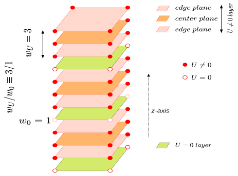
Motivated by the fascinating experimental results in complex oxide superlattices we investigate the magnetotransport properties of the correlated/uncorrelated (antiferromagnetic/paramagnetic) superlattices. In order to explore various phenomena we analyze a range of 3D superlattices based on one band Hubbard model where correlated () layers of width and the uncorrelated () layers of width are periodically arranged as shown in Fig. 1. At half-filling our uncorrelated layers mimics the paramagnetic metallic (PM-M) state where as the correlated layers imitate the antiferromagnetic insulating state (AF-I) layers. Overall, our study unveils the key role of mutual cooperation of the induced magnetic moments in the uncorrelated (paramagnetic) layers and the local moment in the correlated (antiferromagnetic) layers in establishing the antiferromagnetic insulating nature of the whole antiferromagnetic/paramagnetic superlattices. In addition, we emphasize that the induced moments in uncorrelated planes decreases considerably as a function of the distance from the interface. As a result the induced moments completely dissipates with increasing the thickness of uncorrelated layers and nullifies the antiferromagnetic ordering among correlated layers. We comprehensively show that the strength of the local moments and the metal-insulator transition temperature increases as one moves from the edge planes to the center plane in correlated layers.
We organize the paper in the following way: In section II we layout the model Hamiltonian associated with the correlated/uncorrelated superlattices and briefly discuss the numerical methodology. We outline different physical observables to study magnetotransport properties of the antiferromagnetic/paramagnetic SLs in section III. Then in section IV we present the magnetic and transport properties and construct the phase diagrams for different /1 superlattices. We establish the mutual cooperation between the magnetic ordering between the correlated and the uncorrelated layers in section V and present the plane resolved magnetic and transport properties of individual layers in section VI. In section VII we briefly analyze the 1/ SLs and then outline the phase diagram in section VII. We thoroughly study 3/3 SL in section VII. At the end, we summarize our results in section X.
II Model Hamiltonian and Method
To study of the magnetotransport properties of antiferromagnetic/paramagnetic superlattices (SLs) we consider following electron-hole symmetric one orbital Hubbard model:
where is the electron creation (annihilation) operator at site with spin ( or, ) and is the hopping amplitude between the nearest neighbors sites. In the second term is the strength of on-site Coulomb repulsion between two electrons of opposite spin at site and is the spin sum occupation number operator at site . is the chemical potential which controls the overall density of the system. In our electron-hole symmetric model Hamiltonian for half-filling case. Then neglecting the constant term we write down the Hamiltonian in the following form:
where contains the one body part (i.e. quadratic terms) and denotes the interacting part (i.e. quartic term) of the Hamiltonian. Now to solve the Hamiltonian using Monte Carlo method the quartic interaction term can be transformed into combination of two different quadratic terms to set up the Hubbard-Stratonovich (HS) decomposition:
where ; are the Pauli matrices) is the spin at site and is the arbitrary unit vector. The partition function of the model Hamiltonian is written as where and the Boltzmann constant and are set to . The interval is divided into equally spaced slices of width such that . For large values of i.e. in the limit , using Suzuki-Trotter transformation we can write up to first order in . After that by implementing the Hubbard-Stratonovich transformation the interacting part of the partition function for a generic time slice ‘’ can be expressed as
The auxiliary field [] introduced by the Hubbard-Stratonovich decomposition is coupled with the charge density (spin vector ). Now we define a new vector auxiliary field . Finally we obtain the total partition function as
The product follows the time ordered product, where the time slice runs from to . From the partition function we can extract an effective Hamiltonian. At this moment we make two major approximations: (i) by freezing the dependence of the auxiliary fields and retaining the spatial fluctuations of the auxiliary fields, (ii) using the saddle point value of . After all by redefining , we obtain the following effective Hamiltonian Mukherjee ; Chakraborty1 :
| (1) |
We simulate the effective model Hamiltonian using semi-classical Monte Carlo (s-MC) Mukherjee ; Chakraborty1 ; Mukherjee1 ; Patel ; Tiwari method by diagonalizing the fermionic sector in the background of fix and configurations. The classical variables are updated by visiting every lattice site sequentially by implementing metropolis algorithm. We determine self-consistently at every step of the MC system sweep which is then used in the next MC sweeps. We measure physical quantities at every step after the thermal equilibrium to discard illicit correlation in the data. We compute the effective Hamiltonian in a large system size with the help of travelling cluster approximation (TCA) Kumar ; Pradhan ; Chakraborty ; Halder based Monte Carlo technique using TCA cluster.
In the bulk system (where all the sites have finite ), the ground state remains in an antiferromagnetic insulating (AF-I) state for and in a paramagnetic metallic (PM-M) state for , at half-filling. We have designed AF/PM (correlated/uncorrelated) superlattices (SLs) where the AF layer () of width and the PM layer () of width are periodically arranged to form the superlattices. We call the superlattices as SLs, illustrated schematically in Fig. 1. We define () as the fraction of correlated planes in the SL.
III Physical Observables
We evaluate various physical observables to investigate the magnetotransport properties of the whole antiferromagnetic/paramagnetic superlattices. For all superlattices we calculate the layer resolved (separately for correlated layers and uncorrelated layers) observables. In some cases we also calculate plane resolved properties of a given layer (correlated or uncorrelated).
The system averaged magnetization squared is calculated as where . The average magnetic moment irrespective of its direction is inferred from this indicator . The angular brackets represent quantum mechanical and thermal averages throughout the Monte Carlo generated equilibrium configurations. To analyze the long range antiferromagnetic order in superlattices we calculate the structure factor S(q) for as follows:
where is the total number of sites of the system and and run all over the sites of the system. We also calculate the specific heat of the system by differentiating the total energy with respect to temperature, . We apply central difference formula to evaluate the specific heat numerically.
Density of states (DOS) of the system at frequency is determined by using the expression , where are the single particle eigen values and runs over the total number () of eigen values of the system. In our simulation, Lorenzian representation of the delta function with broadening ( is the bare bandwidth) is applied to evaluate the DOS.
The longitudinal (along -axis) and transverse (along -axis) resistivity of the superlattice are calculated by using dc limit of the optical conductivity through Kubo-Greenwood formalism Pradhan ; Mahan ; Kumar1 , represented by
where ( is the lattice parameter). represents the matrix elements of the current operator or, between the eigen states and with corresponding eigen energies and , respectively and is the Fermi function associated with the single particle energy level . Afterwards the dc conductivity is computed by averaging over the low-frequency interval as follows:
where is selected three to five times larger than the average eigen value separation of the system, defined as the ratio of the bare bandwidth to the total number of eigen values. All the physical parameters like , , are measured in units of .
IV Phase diagrams for various superlattices
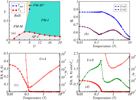
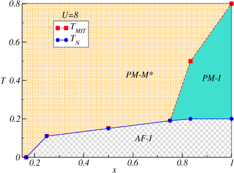
First we briefly discuss the physics of the bulk system ( for all the sites) before analyzing the intriguing phenomena in AF/PM superlattices. We present the phase diagram for bulk system in Fig. 2(a). The ground state of the bulk system shows a G-type antiferromagnetic (G-AF) insulating phase at low temperatures for all values. Please notice that the Neel temperature () varies nonmonotonically with values. Specifically, increases with up to and decreases thereafter. For the system transits from a paramagnetic metallic (PM-M) phase to an AF insulating phase (AF-I) with decreasing the temperature and the metal insulator transition temperature () coincides with the . On the other hand, for or more the system encounters a paramagnetic insulating (PM-I) region above the . As we increase the temperature further the system crosses over to a slightly different kind of paramagnetic metallic phase (abbreviated as PM-M*) above (denoted by dashed line). In order to characterize the properties of PM-M (for 6) and PM-M* (for 8) phases we focus on the vs plot (see Fig. 2(d)). In PM-M* phase (for case), the magnetic moment increases with decreasing temperature whereas the magnetic moment decreases in the PM-M phase (for case) as we go below down to in our phase diagram. In other words local magnetic moments are preformed in PM-M* phase at high temperatures ( 1) unlike the PM-M phase. Although not necessary, we differentiate PM-M and PM-M* phases in the phase diagram for brevity, which will be useful in discussing the phase diagrams of SL systems.
We plot the magnetic and transport properties in Fig. 2(b)-(d) that we used to set up the phase diagram presented in Fig. 2(a). Mainly, we focus on two values ( and ) which represent two different regimes in our phase diagram. As we mentioned earlier the structure factor calculations show that the for is smaller than the for [see Figs. 2(c) and (d)]. The and the of the bulk system are equal to each other for . On the other hand the is much larger than for . A paramagnetic insulating (PM-I) phase intervenes between the PM-M* and AF-I phase at larger values. We also plot the specific heat vs temperature for case in Fig. 2(d). The high-temperature peak associated with charge-fluctuations coincides with the whereas the low-T peak of associated with spin-fluctuations matches well with the Duffy ; Paiva . It is also apparent that, for , the local magnetic moment in PM-M phase decreases upon decreasing the temperature from up to with the enhancement of the metallicity as shown in Fig. 2(b). Below the local magnetic moment increases again with decreasing the temperature. For the magnetic moment gradually increases with decreasing the temperature barring a small peak around and saturates at low temperatures. The small drop just below is due to the delocalization of the electrons assisted by virtual hopping facilitated by the antiferromagnetic correlations. The local moment for both and converge to the asymptotic value at very high temperatures. So, the system directly transforms to an AF-I state from PM-M state upon cooling for whereas the system switches to an AF-I from PM-M* via a PM-I state for larger values as shown in our phase diagram. Overall, the bulk phase diagram obtained in our semi-classical Monte-Carlo (s-MC) approach is consistent with the DQMC Blankenbecler ; Rohringer , 2D cluster-DMFT (C-DMFT) Fratino , 3D cluster-DMFT (C-DMFT) Sato with vortex corrections and QMC simulations Staudt .
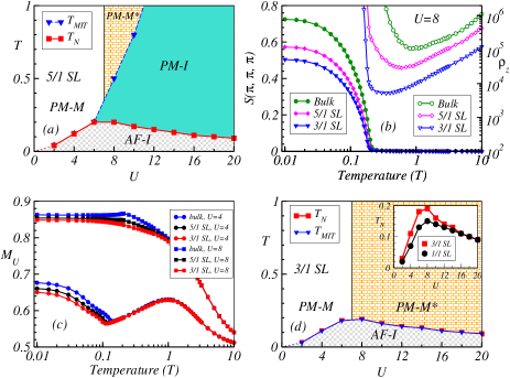
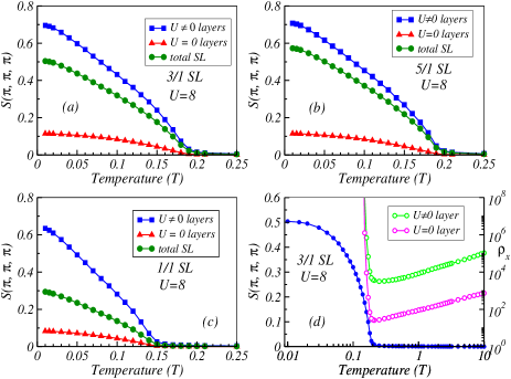
Next, we discuss the phase diagram for different AF/PM superlattices, namely 5/1, 3/1 and 1/1 SLs where ( denotes fraction of correlated planes). We start our analysis with the 5/1 SL [see Fig. 3(a)]. The nonmonotonic behavior of with remains intact for 5/1 SL, similar to the bulk systems although the values decreases very slightly. The for also coincides with the (i.e. the SL system is metallic above the ) and the local magnetic moment decreases as we approach the from the high temperature [see Fig. 3(c) for case]. As a result the PM-M phase, observed in 5/1 SL, remains very similar to the bulk system. PM-M* phase is enlarged for intermediate values as compared to the bulk phase diagram [please compare Fig. 3(a) and Fig. 2(a)]. To analyze the enlarged PM-M* phase further we compare the and obtained from the antiferromagnetic correlations and the resistivity curves, respectively in Fig. 3(b). Interestingly for reduction in is hardly noticeable. On the other hand the decreases considerably due to the insertion of the uncorrelated layers. But, still remains larger than the . Magnetotransport properties of individual layers (comprised of and ) will be discussed later. In this PM-M* phase the magnetic moments in the correlated layer gets more and more localized as we decrease the temperature (see case in Fig. 3(c)] unlike the case.
Now we outline the magnetotransport properties and the phase diagram of 3/1 SL. The profile of 3/1 SL remains more or less the same to that of 5/1 SL (see Fig. 3(d)). We show the comparison of the of 3/1 and 5/1 SLs in Fig. 3(b) for . Interestingly, the coincides with the at in 3/1 SL (unlike 5/1 SL and the bulk systems) as shown in Fig. 3(b). In fact the also coincides with at larger values. As a result the intervening PM-I phase seen between PM-M* and AF-I in 5/1 SL is overtaken by PM-M* phase. So, one directly enters into an antiferromagnetic insulating (AF-I) phase from a paramagnetic metallic (PM-M*) phase in the 3/1 SL system with decrease in temperature. Similar phase diagram is also obtained for the 1/1 SL but the [see the inset of Fig. 3(d)] gets reduced as compared to the 3/1 SL.
V Long range antiferromagnetic ordering: Mutual cooperation between correlated and uncorrelated layers
In this section we analyze the magnetic and transport properties of the individual layers (i.e. separately for correlated () and uncorrelated () layers) of our SL systems to establish a mutual cooperation between the magnetic ordering of the correlated and uncorrelated layers. We plot the local moment profile of the correlated layers for and for 5/1, 3/1 and 1/1 SLs in Fig. 4(a). The local moment (calculated exclusively for correlated layers) gradually increases with decreasing the temperature for both the values and saturates at low temperatures. The local moment in the correlated layer for 1/1 SL is visibly smaller than the 5/1 and 3/1 SLs below . The bidirectional coupling of the correlated plane with the adjacent uncorrelated planes in 1/1 SL suppresses the local moment in the correlated layers. As we increase the values the local moment in the correlated layer for 1/1 SL approaches to that of the 3/1 and 5/1 SLs due to enhancement of the localization in the correlated layers. At low temperature , the local moment of the correlated layers increases monotonically with increase of (since the double occupancy reduces with increase of ) and saturates at large values as shown in Fig. 4(b). But, the local moment in the correlated layer for 1/1 SL is smaller than the 3/1 and 5/1 SLs for intermediate values as mentioned above. Otherwise, the qualitative nature of the local moments profile in the correlated layers remains similar for the 5/1, 3/1 and 1/1 SLs.
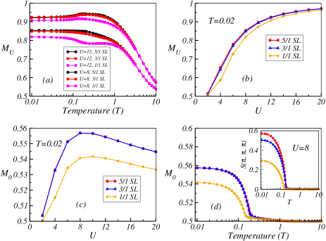
On the other hand, the average induced moment in the uncorrelated layer () shows nonmonotonic behavior with increase of values and the maximum moment is obtained for for all the three SLs [see Fig. 4(c)]. These induced moments in the uncorrelated layer are generated due to the kinetic hopping of the charge carriers from the correlated layers. In addition, it is apparently clear that the induced moment in uncorrelated layers for 1/1 SL is substantially smaller than the 3/1 and 5/1 superlattices. The induced magnetic moment in the uncorrelated layer is similar to the experimentally observed induced magnetic moment in the paramagnetic layer in NiO/Pd multilayers Saha ; Manago ; Manago1 ; Manago2 ; Manago3 and the induced magnetic moment in layer in CuO/Cu multilayers Munakata .
In order to extract the temperature scale at which magnetic moments are actually induced in the uncorrelated layers we plot the local moment of uncorrelated layers vs temperature for 5/1, 3/1, and 1/1 SLs for case in Fig. 4(d). Local moments are induced in the uncorrelated layer at very low temperatures (the temperature where becomes greater than 0.5) as compared to the correlated layers. The onset temperature of the induced moment in the uncorrelated layer () around matches well with the of these SL systems (see the inset of Fig. 4(d)). So our calculations show a one-to-one correspondence between antiferromagnetic ordering and onset of induced moments in uncorrelated layers in the SL systems.
To further analyze the correspondence between the onset of antiferromagnetic ordering in correlated and uncorrelated layers we plot structure factor of both the layers separately and compare it with the structure factor of the total SL system in Figs. 5(a)-(c). The structure factors show that the antiferromagnetic order appears at the same temperature for both correlated layers ( layers) and uncorrelated layers ( layers) and matches well with the of the whole superlattice system. This also indicates that the correlations among the induced moments in the uncorrelated layer play an important role in mediating the long range interactions between the correlated layers. So, overall the cooperation between the correlated and uncorrelated layers helps to sustain the global long range AF order in the superlattices. We also plot the layer resolved resistivities for the 3/1 SL in Fig. 5 (d). of whole 3/1 SL is re-plotted in the same figure for comparing the transition temperatures. The obtained from correlated layers and uncorrelated layers are equal to each other and coincides with the for the SL system.
VI Plane resolved transport properties of the superlattices
Here, we investigate the plane resolved transport properties of the correlated and uncorrelated layers of the superlattices. First we focus on 3/1 SL where only one uncorrelated plane () is intercalated between the correlated layers made up of three correlated planes. For this we evaluate the in-plane resistivity () of individual planes (three correlated planes and one uncorrelated plane) for as shown in Fig. 6(a). Interestingly, the metal-insulator transition temperature of the edge correlated planes () is smaller than the center () correlated planes (i.e, ) in 3/1 SL. It is clearly observed that the center correlated plane exhibits MIT above whereas the of both the edge planes coincides with the . The of the uncorrelated plane also matches with the . Expectedly the value of in the uncorrelated plane is much smaller than the correlated plane.
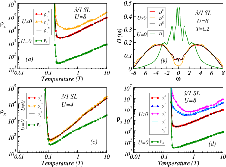
Next, we calculate plane-resolved density of states (DOS) to further deliberate the transport properties. Plane-resolved DOS of the correlated layer at (see Fig. 6(b)) indicate that weight of the DOS of the edge correlated planes at the Fermi level (set at ) are larger as compared to the central correlated plane (i.e. at ). Expectedly the weight of DOS of the uncorrelated plane at Fermi level is significantly greater than all the correlated planes. Hence, our plane-resolved DOS calculations are coherent with the in-plane resistivity calculations of the individual planes of the superlattice.
For smaller values all the planes (comprised of three correlated planes and one uncorrelated plane) show metal-insulator transition at the same temperature [see Fig. 6(c)] and this temperature coincides with the . In fact, the resistivity curves of all three correlated planes overlap with each other. This shows that all the correlated planes are equally affected by the insertion of uncorrelated layer for smaller values where moments are much more delocalized as compared to higher values. Our magnetotransport results qualitatively follow the QMC Jiang and DQMC Euverte studies of the correlated superlattices where it was shown that the correlated layer is affected by the uncorrelated layer and the effect increases with decrease of . But, the detailed transport properties were not reported earlier. The transport properties of 5/1 SL [see Fig. 6(d)] remains qualitatively similar to that of 3/1 SL where the increases as we move from the edge plane to the center plane.
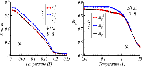
In our 3/1 SL the correlated layer is made up of three planes. So the obvious question arises at this point: Does all the three correlated planes (two edge planes and one center plane) that constitute the correlated layer align antiferromagntically at the same temperature or not? To answer this question we plot the antiferromagnetic structure factor of all the three correlated planes separately using in Fig. 7(a). The AF correlations of individual planes vanish at the same temperature. But, the reduction in the low-temperature saturation value in edge plane as compared to center plane is very clear. This may be due to the larger magnetic moment in the center plane than the edge planes. To confirm this we plot the local magnetic moment of individual correlated planes vs temperature in Fig. 7(b). In fact, the for the center plane is larger than the edge plane at low temperatures.
The uncorrelated plane affects the local magnetic moments of the correlated planes differently ( is larger for central plane) due to the proximity effect as we discussed earlier. Apparently the profiles indicate that the resulting effective () of center plane is larger than the edge plane. This is also supported from resistivity plots where of the center plane is larger than the edge plane (see Fig. 6 (a)). From all these analysis one would naively expect that the of the edge plane should be smaller than the center plane but this difference is beyond the resolution of our calculations and we get more or less same [see Fig. 7(a)].
VII Magnetotransport properties of 1/3 and 1/5 superlattices
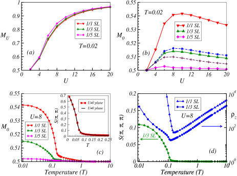
Now we briefly analyze the transport and magnetic properties of 1/3 and 1/5 SLs to present a diagram. We plot the local moment of the correlated layers for 1/1, 1/3 and 1/5 SLs with different values at . The local moments of the correlated layers increases monotonically with increase of and saturates at large values as shown in Fig. 8(a) for all three SLs. So, the qualitative nature of the local moments profile in the correlated planes remains the same as we increase the thickness of uncorrelated layer. We also plot the induced magnetic moment in uncorrelated layers in Fig. 8(b). Induced magnetic moment shows nonmonotonic behavior for 1/1 and 1/3 SLs. But, induced magnetic moment decreases drastically for 1/5 SL. The average induced moment in the edge and center uncorrelated () planes are also plotted (see Fig. 8(b)) for 1/3 SL. The nonmonotonic behavior remains intact for both edge and center plane and expectedly the induced moment in the edge uncorrelated plane is larger than the center uncorrelated plane.
The induced moments in the uncorrelated layer decreases as we shift from 1/1 to 1/3 SL as shown in Fig. 8(b). But, there is a clear onset temperature of the induced moment in the uncorrelated layer () around for 1/3 SL as shown in Fig. 8(c). So, one expect long range antiferromagnetic correlations in 1/3 SL. In fact, magnetic structure factor S(,,) for 1/3 SL (see Fig. 8(d)) shows that the SL system is antiferromagnetic at low temperatures. Resistivity curve, plotted in same figure, shows that the matches well with the . Expectedly the resistivity of 1/3 SL is much lower than the 1/1 SL due to participations of thicker uncorrelated layer (see Fig. 8(d)).
Does the 1/5 SL system have an antiferromagnetic ordering at low temperatures? Our calculations show that the induced moment in uncorrelated layers for 1/5 SL is negligible (see Fig. 8 (b) and (c)) and as result the long range antiferromagnetic correlation between the correlated layers cease to exist. To gain more insight of magnetic correlations of correlated planes separated by five uncorrelated planes we plot the magnetic structure factor S(,) for individual correlated planes in the inset of Fig. 8(c). It is apparent that the individual correlated layers are antiferromagnetically ordered by themselves but due to insufficient induced moments in uncorrelated planes the long range antiferromagnetic order between them is not established.
VIII phase diagram
Thereafter, we present the phase diagram for the correlated/uncorrelated SLs for where = 1 or/and = 1. The Neel temperature [from plots] and the metal-insulator transition temperature [from plot] for different SLs are used to construct this phase diagram. Fraction of correlated planes is varied in our SLs. We plot the for 1/5 SL (), 1/3 SL (), 1/1 SL (), 3/1 SL (), 5/1 SL () and bulk () in Fig. 9. For bulk case () the system transits from PM-I phase to an AF-I phase as we discussed earlier. This PM-I to AF-I transition remains intact for 5/1 SL () although the decreases considerably. For the PM-I phase above AF-I phase disappears and as a result the matches well with the . Lastly, the antiferromagnetic ordering vanishes for 1/5 SL (i.e. for ). So, to summarize, the superlattice system directly transits from AF-I state to - state with increase of temperature for whereas the SL system converts to - state from AF-I state via the PM-I state upon increasing the temperature for at . This phase diagram is similar to the very recently reported phase diagram in Ref. 72, where randomly diluted systems were studied.
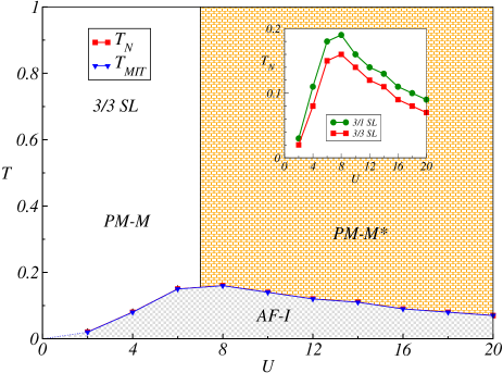
IX Magnetotransport properties of 3/3 SL
Now we proceed to study the plane resolved magnetic and transport properties for 3/3 SL ( = 0.5). First, we plot the phase diagram for 3/3 SL in Fig. 10. This phase diagram is very similar to 3/1 and 1/1 SLs that we presented in Fig. 3(d). We plot the antiferromagnetic structure factor and resistivities ( and ) for the 3/3 SL in Fig. 11(a) for . The of 3/3 SL remains more or less same to that of 1/1 SL. The obtained from and are also equal to each other and matches well with the . Obviously, the value of out-of-plane resistivity is larger than in-plane resistivity . The plane resolved resistivities of the correlated and uncorrelated layers are shown in Fig. 11(b). The of central correlated plane is larger than the edge correlated planes. Interestingly, only the of the edge correlated plane matches with the . On the other hand, all the uncorrelated planes show the metal-insulator transition at . In addition it is clear that the central correlated (uncorrelated) plane is more (less) resistive than the edge correlated (uncorrelated) planes in correlated (uncorrelated) layer. The coupling of the correlated edge plane with the nearest uncorrelated plane reduces its resistivity as compared to the central correlated plane. In other words metallicity penetrates to the correlated edge layer above the due to the interfacial coupling between the correlated and uncorrelated layers. This interfacial coupling is also reflected in the plane resolved magnetic moments profile of the correlated layer shown in Fig. 11(c). We find that the center plane has larger moment as compared to the edge planes at low temperatures. Expectedly the edge plane of the uncorrelated layer also has comparatively larger induced magnetic moment to that of center plane as shown in the same figure.
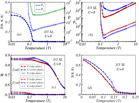
Now, the same question that we addressed for 3/1 SL arises here: Does all the three correlated planes (two edge planes and one center plane) that constitute the correlated layer in the 3/3 SL align antiferromagntically at the same temperature? To answer this question we plot the antiferromagnetic structure factor of the three correlated planes for in Fig. 11(d). The of the center plane is slightly higher than the edge planes which is expected. So, one can firmly claim that the effective () of the central plane is somewhat larger than the edge planes.
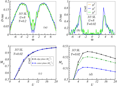
To analyze the plane resolved magnetic and transport properties further we have calculated the density of states (DOS) of the individual correlated planes of the 3/3 SL. The DOS () of the individual planes of the correlated layer are shown in Fig. 12(a) for at temperature (just above ). Emergence of Mott lobes at is apparent in all the three correlated planes. But the weight of DOS at the Fermi level () for the edge correlated plane is comparatively larger than to that of the central correlated plane. This larger weight at the Fermi level enforces the edge correlated planes to have smaller resistivity than the center correlated plane. At low temperature a clear Mott gap opens in the DOS of center correlated plane as shown in Fig. 12(b). Although same kind of gap is noticed for both the edge plane and center plane, some very tiny satellite patterned structures appear in the band-gap of edge planes.
At low temperatures () the local moment of the correlated planes increases monotonically with increase of and saturates at large values as shown in Fig. 12(c). The local moments in the center plane is slightly larger than the edge plane for intermediate values. Otherwise, the qualitative monotonic nature of the local moments profile in the correlated planes remains the same. On the other hand the induced magnetic moment in uncorrelated layer shows nonmonotonic behavior (for both edge and center plane) with at low temperatures. The induced local moment in the edge uncorrelated plane is significantly larger than the center uncorrelated plane as shown in Fig. 12(d). This is due to the fact that the uncorrelated edge plane which is adjacent to the correlated plane gets more affected by the correlated layer.
X Conclusions
In this paper we have implemented one band Hubbard model at half-filling to investigate the AF/PM superlattices by using semi-classical Monte Carlo approach. We analyze various superlattices in three dimensions where correlated (with on-site repulsion strength ) and uncorrelated ( = 0) layers are arranged periodically. First, we explore the phase diagrams for various /1 SLs ( = 5, 3, 1) and compare the results with the bulk systems. We show that the magnetic moments are induced in the uncorrelated layers at low temperatures due to the kinetic hopping of carriers and optimum magnetic moment is induced for . The antiferromagnetic ordering among the induced moments in uncorrelated layers mediates the long range antiferromagnetic ordering between the correlated layers and as a result the antiferromagnetic insulating nature of the bulk systems remains intact in the SLs. In other words, the long range antiferromagnetic order survives in the superlattices through the mutual cooperation of the induced moment in the uncorrelated layer and the local moment in the correlated layer. Thus, the induced moments in the uncorrelated layer play an important role in determining the global long range antiferromagnetic order in the superlattices.
To analyze the plane resolved magnetotransport properties we focus on the regime. Interestingly, the average local moments in the edge planes are comparatively smaller than the central plane in the correlated layer. The coupling of the edge planes of correlated and uncorrelated layers reduces the local magnetic moments of the edge correlated plane but induces magnetic moments in uncorrelated layer. In-plane resistivity calculations of the individual constituent planes of the superlattices show that the increases as we move from edge plane to center plane inside the correlated layers, which is consistent with the local moment profile of the individual constituent planes. So overall our plane resolved calculations establish an one-to-one connection between the local moment profile and the in-plane transport properties of the superlattices. Plane-resolved density of states calculations of the individual planes of the correlated layer are also concomitant with the in-plane resistivities. On the other hand the induced moments in uncorrelated planes decreases considerably as a function of the distance from the interface, but the metal-insulator transition temperature of edge and center planes remain more or less unaffected. In the end, we show that the induced moments in uncorrelated layers dissipates with increasing the thickness of uncorrelated layers as a result the antiferromagnetic ordering among correlated layers vanishes.
ACKNOWLEDGMENT
We acknowledge use of the Meghnad2019 computer cluster at SINP.
References
- (1) H. Y. Hwang, Y. Iwasa, M. Kawasaki, B. Keimer, N. Nagaosa, and Y. Tokura, Nat. Mater. 11, 103 (2012).
- (2) J. Chakhalian, A. J. Millis, and J. Rondinelli, Nat. Mater. 11, 92 (2012).
- (3) J. Chakhalian, J. W. Freeland, A. J. Millis, C. Panagopoulos, and J. M. Rondinelli, Rev. Mod. Phys. 86, 1189 (2014).
- (4) A. Bhattacharya and S. J. May, Annu. Rev. Mater. Res. 44, 65 (2014).
- (5) P. Zubko, S. Gariglio, M. Gabay, P. Ghosez, and J. M. Triscone, Annu. Rev. Condens. Matter Phys. 2, 141 (2011).
- (6) D. G. Schlom, D. G., L.-Q. Chen, X. Pan, A. Schmehl, and M. A. Zurbuchen, J. Am. Ceram. Soc. 91, 2429 (2008).
- (7) S. Middey, J. Chakhalian, P. Mahadevan, J.W. Freeland, A.J. Millis, and D.D. Sarma, Annu. Rev. Mater. Res. 46, 305 (2016).
- (8) J. Stahn, J. Chakhalian, C. Niedermayer, J. Hoppler, T. Gutberlet, J. Voigt, F. Treubel, H.-U. Habermeier, G. Cristiani, B. Keimer, and C. Bernhard, Phys. Rev. B 71, 140509(R) (2005).
- (9) J. Chakhalian, J. W. Freeland, G. Srajer, J. Strempfer, G. Khaliullin, J. C. Cezar, T. Charlton, R. Dalgliesh, C. Bernhard, G. Cristian, H. -U. Habermeier, and B. Keimer, Nat. Phys. 2, 244 (2006).
- (10) K. S. Takahashi, M. Kawasaki, Y. Tokura, Appl. Phys. Lett. 79, 1324 (2001).
- (11) A. V. Boris, Y. Matiks, E. Benckiser, A. Frano, P. Popovich, V. Hinkov, P. Wochner, M. Castro-Colin, E. Detemple, V. K. Malik, C. Bernhard, T. Prokscha, A. Suter, Z. Salman, E. Morenzoni, G. Cristiani, H. -U. Habermeier, B. Keimer, Science 332, 937 (2011).
- (12) S. Okamoto, and A. Millis, Nature 428, 630 (2004).
- (13) S. Okamoto, Phys. Rev. B 82, 024427 (2010).
- (14) Y. Cao, Xiaoran Liu, M. Kareev, D. Choudhury, S. Middey, D. Meyers, J. -W. Kim, P. J. Ryan, J. W. Freeland, and J. Chakhalian, Nat. Commun. 7, 10418 (2016).
- (15) X. R. Wang, C. J. Li, W. M. Lü, T. R. Paudel, D. P. Leusink, M. Hoek, N. Poccia, A. Vailionis, T. Venkatesan, J. M. D. Coey, E. Y. Tsymbal, Ariando, and H. Hilgenkamp, Science 349, 716 (2015).
- (16) F. Y. Bruno, J. Garcia-Barriocanal, M. Varela, N. M. Nemes, P. Thakur, J. C. Cezar, N. B. Brookes, A. Rivera-Calzada, M. Garcia-Hernandez, C. Leon, S. Okamoto, S. J. Pennycook, and J. Santamaria, Phys. Rev. Lett. 106, 147205 (2011).
- (17) J. S. Lee, D. A. Arena, P. Yu, C. S. Nelson, R. Fan, C. J. Kinane, S. Langridge, M. D. Rossell, R. Ramesh, and C. C. Kao, Phys. Rev. Lett. 105, 257204 (2010).
- (18) A. Tebano, A. Orsini, P. G. Medaglia, D. DiCastro, G. Balestrino, B. Freelon, A. Bostwick, Y. J. Chang, G. Gaines, E. Rotenberg, and N. L. Saini, Phys. Rev. B 82, 214407 (2010).
- (19) A. Tebano, C. Aruta, S. Sanna, P. G. Medaglia, G. Balestrino, A. A. Sidorenko, R. DeRenzi, G. Ghiringhelli, L. Braicovich, V. Bisogni, and N. B. Brookes, Phys. Rev. Lett. 100, 137401 (2008).
- (20) J. Chakhalian, J. W. Freeland, H.-U. Habermeier, G. Cristiani, G. Khaliullin, M. van Veenendaal, B. Keimer Chakhalian, Science 318, 1114 (2007).
- (21) J. J. Peng, C. Song, F. Li, B. Cui, H. J. Mao, Y. Y. Wang, G. Y. Wang, F. Pan, ACS Appl. Mater. Interfaces 7, 17700 (2015).
- (22) J. Liu, S. Okamoto, M. van Veenendaal, M. Kareev, B. Gray, P. Ryan, J. W. Freeland, and J. Chakhalian, Phys. Rev. B 83, 161102 (2011).
- (23) J. Liu, M. Kareev, D. Meyers, B. Gray, P. Ryan, J. W. Freeland, and J. Chakhalian, Phys. Rev. Lett. 109, 107402 (2012).
- (24) H. Chen, D. P. Kumah, A. S. Disa, F. J. Walker, C. H. Ahn, and S. Ismail-Beigi, Phys. Rev. Lett. 110, 186402 (2013).
- (25) M. C. Dekker, A. Herklotz, L. Schultz, M. Reibold, K. Vogel, M. D. Biegalski, H. M. Christen, and K. Dorr, Phys. Rev. B 84, 054463 (2011).
- (26) H. Boschker, J. Kautz, E. P. Houwman, W. Siemons, D. H. A. Blank, M. Huijben, G. Koster, A. Vailionis, and G. Rijnders, Phys. Rev. Lett. 109, 157207 (2012).
- (27) X. Li, I. L. Vrejoiu, M. Ziese, A. Gloter, and P. A. van Aken, Scientific Reports 7, 40068 (2017).
- (28) S. J. May, P. J. Ryan, J. L. Robertson, J. -W. Kim, T. S. Santos, E. Karapetrova, J. L. Zarestky, X. Zhai, S. G. E. te Velthuis, J. N. Eckstein, S. D. Bader, and A. Bhattacharya, Nat. Mater. 8, 892 (2009).
- (29) Q. H. Qin, L. Äkäslompolo, N. Tuomisto, L. Yao, S. Majumdar, J. Vijayakumar, A. Casiraghi, S. Inkinen, B. Chen, A. Zugarramurdi, M. Puska, and S. van Dijken, Adv. Mater. 28, 6852 (2016).
- (30) M. N. Grisolia, J. Varignon, G. Sanchez-Santolino, A. Arora, S. Valencia, M. Varela, R. Abrudan, E. Weschke, E. Schierle, J. E. Rault, J. -P. Rueff, A. Barthélémy, J. Santamaria and M. Bibes, Nat. Phys. 12, 484 (2016).
- (31) A. Ohtomo, H. Y. Hwang, Nature 427, 423 (2004).
- (32) A. Brinkman, M. Huijben, M. V. Zalk, J. Huijben, U. Zeitler, J. C. Maan, W. G. V. der Wiel, G. Rijnders, D. H. A. Blank, and H. Hilgenkamp, Nat. Mater. 6, 493 (2007).
- (33) N. Reyren, S. Thiel, A. D. Caviglia, L. Fitting-Kourkoutis, G. Hammerl, C. Richter, C. W. Schneider, T. Kopp, A. S. Ruetschi, D. Jaccard, M. Gabay, D. A. Muller, J. M. Triscone, and J. Mannhart, Science 317, 1196 (2007).
- (34) A. Ohtomo, D. A. Muller, J. L. Grazul, H. Hwang, Nature 419, 378 (2002).
- (35) J. Zheng, W. Shi, Z. Li, J. Zhang, C. -Y. Yang, Z. Zhu, M. Wang, J. Zhang, F. Han, H. Zhang, Y. Chen, F. Hu, B. Shen, Y. Chen, and J. Sun, ACS Nano 18, 9232 (2024).
- (36) Y. Takamura, F. Yang, N. Kemik, E. Arenholz, M. D. Biegalski, and H. M. Christen, Phys. Rev. B 80, 180417(R) (2009).
- (37) J. D. Hoffman, B. J. Kirby, J. Kwon, Gilberto Fabbris, D. Meyers, J. W. Freeland, I. Martin, O. G. Heinonen, P. Steadman, H. Zhou, C. M. Schlepütz, M. P. M. Dean, S. G. E. te Velthuis, J. -M. Zuo, and A. Bhattacharya, Phys. Rev. X 6, 041038 (2016).
- (38) J. Garcia-Barriocanal, J. C. Cezar, F. Y. Bruno, P. Thakur, N. B. Brookes, C. Utfeld, A. Rivera-Calzada, S. R. Giblin, J. W. Taylor, J. A. Duffy, S. B. Dugdale, T. Nakamura, K. Kodama, C. Leon, S. Okamoto, and J. Santamaria, Nat. Commun. 1, 82 (2010).
- (39) N. Nakagawa, H. Y. Hwang, D. A. Muller, Nat. Mater. 5, 204 (2006).
- (40) T. Koida, M. Lippmaa, T. Fukumura, K. Itaka, Y. Matsumoto, M. Kawasaki, and H. Koinuma, Phys. Rev. B 66, 144418 (2002).
- (41) A. Gozar, G. Logvenov, L. Fitting Kourkoutis, A. T. Bollinger, L. A. Giannuzzi, D. A. Muller, I. Bozovic, Nature 455, 782 (2008).
- (42) D. A. Dikin, M. Mehta, C. W. Bark, C. M. Folkman, C. B. Eom, and V. Chandrasekhar, Phys. Rev. Lett. 107, 056802 (2011).
- (43) L. Li, C. Richter, J. Mannhart, and R. C. Ashoori, Nat. Phys. 7, 762 (2011).
- (44) J. A. Bert, B. Kalisky, C. Bell, M. Kim, Y. Hikita, H. Y. Hwang, and K. A. Moler, Nat. Phys. 7, 767 (2011).
- (45) S. S. A. Seo, W. S. Choi, H. N. Lee, L. Yu, K. W. Kim, C. Bernhard, T. W. Noh, Phys. Rev. Lett. 99, 266801 (2007).
- (46) G. Zhou, C. Song, Y. Bai, Z. Quan, F. Jiang, W. Liu, Y. Xu, S. S. Dhesi, X. Xu, ACS Appl. Mater. Interfaces 9, 3156 (2017).
- (47) M. Gibert, P. Zubko, R. Scherwitzl, J. niguez, J. -M. Triscone, Nat. Mater. 11, 195 (2012).
- (48) M. Gibert, M. Viret, A. Torres-Pardo, C. Piamonteze, P. Zubko, N. Jaouen, J. -M. Tonnerre, A. Mougin, J. Fowlie, S. Catalano, A. Gloter, O. Stephan, and J. -M. Triscone, Nano Lett. 15, 7355 (2015).
- (49) A. T. Lee, M. J. Han, Phys. Rev. B 88, 035126 (2013).
- (50) S. Dong, E. Dagotto, Phys. Rev. B 87, 195116 (2013).
- (51) J. Hoffman, I. C. Tung, B. B. Nelson-Cheeseman, M. Liu, J. W. Freeland, A. Bhattacharya, Phys. Rev. B 88, 144411 (2013).
- (52) C. Piamonteze, M. Gibert, J. Heirdler, S. Rusponi, H. Brune, H. -M. Triscone, F. Nolting, U. Staub, Phys. Rev. B 92, 014426 (2015).
- (53) A. J. Grutter, H. Yang, B. J. Kirby, M. R. Fitzsimmons, J. A. Aguiar, N. D. Browning, C. A. Jenkins, E. Arenholz, V. V. Mehta, U. S. Alaan, and Y. Suzuki, Phys. Rev. Lett. 111, 087202 (2013).
- (54) J. Mannhart and D. G. Schlom, Sciences 327, 1607 (2010).
- (55) J. Garcia-Barriocanal, F. Y. Bruno, A. Rivera-Calzada, Z. Sefrioui, N. M. Nemes, M. Garcia-Hernandez, J. Rubio-Zuazo, G. R. Castro, M. Varela, S. J. Pennycook, C. Leon, and J. Santamaria, Adv. Mater. 22, 627 (2010).
- (56) J. Jilili, F. Cossu, and U. Schwingenschlögl, Scientific Reports 5, 13762 (2015).
- (57) F. Cossu, J. Jilili, and U. Schwingenschlögl, Adv. Mater. Interfaces 1, 1400057 (2014).
- (58) J. Chaloupka, G. Khaliullin, Phys. Rev. Lett. 100, 016404 (2008).
- (59) T. Nguyen, V. H. Huang, T. -Y. Koo, N. -S. Lee, and H. -J. Kim, Scientific Reports 9, 20145 (2019).
- (60) H. Shishido, T. Shibauchi, K. Yasu, T. Kato, H. Kontani, T. Terashima, and Y. Matsuda, Science 327, 980 (2010).
- (61) S. K. Saha, V. S. Stepanyuk, and J. Kirschner, Physics Letters A 378, 3642 (2014).
- (62) T. Manago, T. Ono, H. Miyajima, K. Kawaguchi, and M. Sohma, J. Phys. Soc. Japan 68, 3677 (1999).
- (63) T. Manago, T. Ono, H. Miyajima, K. Kawaguchi, M. Sohma, J. Phys. Soc. Japan 68, 334 (1999).
- (64) T. Manago, T. Ono, H. Miyajima, K. Kawaguchi, M. Sohma, Solid State Commun. 109, 621 (1999).
- (65) T. Manago, H. Miyajima, K. Kawaguchi, M. Sohma, I. Yamaguchi, J. Magn. Magn. Mater. 177, 1191 (1998).
- (66) K. Munakata, T. H. Geballe, and M. R. Beasley, Phys. Rev. B 84, 161405(R) (2011).
- (67) M. Jiang, G. G. Batrouni, and R. T. Scalettar, Phys. Rev. B 86, 195117 (2012).
- (68) A. Zujev and P. Sengupta, Phys. Rev. B 88, 094415 (2013).
- (69) A. Euverte, F. Hebert, S. Chiesa, R. T. Scalettar, and G. G. Batrouni Phys. Rev. Lett. 108, 246401 (2012).
- (70) R. Mondaini and T. Paiva, Phys. Rev. B 95, 075142 (2017).
- (71) A. Mukherjee, N. D. Patel, S. Dong, S. Johnston, A. Moreo, and E. Dagotto, Phys. Rev. B 90, 205133 (2014).
- (72) S. Chakraborty, A. Mukherjee, and K. Pradhan, Phys. Rev. B 106, 075146 (2022).
- (73) A. Mukherjee, N. D. Patel, C. Bishop, and E. Dagotto, Phys. Rev. E 91, 063303 (2015).
- (74) N. D. Patel, A. Mukherjee, N. Kaushal, A. Moreo, and E. Dagotto, Phys. Rev. Lett. 119, 086601 (2017).
- (75) R. Tiwari and P. Majumdar, Europhys. Lett. 108, 27007 (2014).
- (76) S. Kumar, P. Majumdar, Eur. Phys. J. B 50, 571 (2006).
- (77) K. Pradhan and A. P. Kampf, Phys. Rev. B 87, 155152 (2013).
- (78) S. Chakraborty, S. Halder, and K. Pradhan, Phys. Rev. B 108, 165110 (2023)
- (79) S. Halder, Subrat K. Das, and K. Pradhan, Phys. Rev. B 108, 235111 (2023).
- (80) G. D. Mahan, Quantum Many Particle Physics (Plenum, New York, 1990).
- (81) S. Kumar and P. Majumdar, Europhys. Lett. 65, 75 (2004).
- (82) D. Duffy and A. Moreo, Phys. Rev. B 55, 12918 (1997).
- (83) T. Paiva, R. T. Scalettar, C. Huscroft, and A. K. McMahan, Phys. Rev. B 63, 125116 (2001).
- (84) R. Blankenbecler, D. J. Scalapino, and R. L. Sugar, Phys. Rev. D: Part. Fields 24, 2278 (1981).
- (85) G. Rohringer, A. Toschi, A. A. Katanin, and K. Held, Phys. Rev. Lett. 107, 256402 (2011).
- (86) L. Fratino, P. Semon, M. Charlebois, G. Sordi, and A. M. S. Tremblay, Phys. Rev. B 95, 235109 (2017).
- (87) T. Sato and H. Tsunetsugu, Phys. Rev. B 94, 085110 (2016).
- (88) R. Staudt, M. Dzierzawa, and A. Muramatsu, Eur. Phys. J. B 17, 411 (2000).