A Finite Element Method by Patch Reconstruction for the Quad-Curl Problem Using Mixed Formulations

Abstract.

We develop a high order reconstructed discontinuous approximation (RDA) method for solving a mixed formulation of the quad-curl problem in two and three dimensions. This mixed formulation is established by adding an auxiliary variable to control the divergence of the field. The approximation space for the original variables is constructed by patch reconstruction with exactly one degree of freedom per element in each dimension and the auxiliary variable is approximated by the piecewise constant space. We prove the optimal convergence rate under the energy norm and also suboptimal $L^{2}$ convergence using a duality approach. Numerical results are provided to verify the theoretical analysis.
keywords: quad-curl problem, mixed formulation, patch reconstruction

1. Introduction

The quad-curl problem arises in many multiphysics simulations, especially in inverse electromagnetic scattering for inhomogeneous media ,magnetohydrodynamics and also Maxwell transmission eigenvalue problems. Therefore, it is important to design highly efficient and accurate numerical methods for quad-curl problems.

Finite element methods (FEMs) are a widely used numerical scheme for solving partial differential equations. The presence of the quad-curl operator makes it difficult and challenging to design the conforming finite element space for quad-curl problems. We refer to [21, 10, 22] for somes recent works in constructing $H(\mathrm{curl}^{2})$-conforming finite element spaces in two and three dimensions. Due to the difficulties in discretizations of the quad-curl operator, much attentions have been paid on using nonconforming elements such as Nédélec ’s elements and completely discontinuous piecewise polynomials. We refer to [24, 9, 7] and the reference therein for works of this type. Another approach is devoted to mixed formulations. Some discussions can be found in [23, 19, 18]. Specifically, [23] reduces the original problem to systems of low order equations by introducing intermediate variables, which makes the solution easier to approximate.

In this paper, we propose a mixed discontinuous Galerkin finite element method for the quad-curl problem with divergence-free variable. A significant drawback of DG space is the large number of degrees of freedom in DG space, which results in high computational costs. This drawback is a matter of concern. We follow the methodology in [13, 12, 14, 11] to apply the patch reconstruction finite element method to the quad-curl problem. The construction of the approximation space includes creating an element patch for each element and solving a local least squares problem to obtain a polynomial basis function locally. Methods based on the reconstructed spaces are called reconstructed discontinuous approximation methods, which can approximate functions to high-order accuracy meanwhile inherits the flexibility on the mesh partition. One advantage of this space is that it has very few degrees of freedom, which gives high approximation efficiency of finite element. The reconstructed space is a subspace of the standard DG space, so that we can borrow ideas from the interior penalty formulations to solve the quad-curl problem. For the auxiliary variable, we use the piecewise constant space as the approximation space. Therefore, the mixed systems not grow much in size compared to the original system. By adding penalty terms for both spaces, we do not need the two space to satisfy the discrete inf-sup condition. We prove the convergence rates under the energy norm and the $L^{2}$ norm, and numerical experiments are conducted to verify the theoretical analysis and show that our algorithm is simple to implement and can reach high-order accuracy.

The rest of this paper is organized as follows. In Section 2, we introduce the quad-curl problem with div-free condition and give the basic notations about the Sobolev spaces and the partition. In Section 3, we introdude the RDA based finite element method. In Section 4, we describe the mixed finite element method for the quad-curl problem, and prove that the convergence rate is optimal with respect to the energy norm and suboptimal with respect to the $L^{2}$ norm. In Section 5, we carry out some numerical examples to verify our theoretical results. A brief conclusion is given in Section 6.

2. preliminaries

Let $\Omega\subset\mathbb{R}^{d}(d=2,3)$ be a bounded polygonal (polyhedral) domain with a Lipschitz boundary $\partial\Omega$.

Given $\boldsymbol{f}\in H(\mathrm{div}^{0},\Omega)$, we consider the following quad-curl problem

(1) $$\left\{\begin{aligned} \mathrm{curl}^{4}\boldsymbol{u}=\boldsymbol{f},&\quad\text{ in }\Omega,\\ \nabla\cdot\boldsymbol{u}=0,&\quad\text{ in }\Omega,\\ \boldsymbol{u}\times\boldsymbol{n}=0,&\quad\text{ on }\partial\Omega,\\ (\nabla\times\boldsymbol{u})\times\boldsymbol{n}=0,&\quad\text{ on }\partial\Omega,\end{aligned}\right.$$

We introduce an auxiliary variable $p$ to rewrite the problem as

(2) $$\left\{\begin{aligned} \mathrm{curl}^{4}\boldsymbol{u}+\nabla p=\boldsymbol{f},&\quad\text{ in }\Omega,\\ \nabla\cdot\boldsymbol{u}=0,&\quad\text{ in }\Omega,\\ \boldsymbol{u}\times\boldsymbol{n}=0,&\quad\text{ on }\partial\Omega,\\ (\nabla\times\boldsymbol{u})\times\boldsymbol{n}=0,&\quad\text{ on }\partial\Omega,\\ p=0,&\quad\text{on }\partial\Omega.\end{aligned}\right.$$

The weak form to the problem (2) is to find $(\boldsymbol{u},p)\in H_{0}(\mathrm{curl}^{2},\Omega)\times H_{0}^{1}(\Omega)$ such that

$$(\mathrm{curl}^{2}\boldsymbol{u},\mathrm{curl}^{2}\boldsymbol{v})+(\boldsymbol{v},\nabla p) =(\boldsymbol{f},\boldsymbol{v}),\ \forall\boldsymbol{v}\in H_{0}(\mathrm{curl}^{2},\Omega),$$

$$-(\boldsymbol{u},\nabla q) =0,\ \forall q\in H_{0}^{1}(\Omega),$$

For the problem domain $\Omega$, we define

$$H(\mathrm{curl}^{s},\Omega) :=\left\{\boldsymbol{v}\in L^{2}(\Omega)^{d}\ |\ \mathrm{curl}^{j}\boldsymbol{v}\in L^{2}(\Omega),1\leq j\leq s\right\},$$

$$H_{0}(\mathrm{curl}^{s},\Omega) :=\left\{\boldsymbol{v}\in L^{2}(\Omega)^{d}\ |\ \mathrm{curl}^{j}\boldsymbol{v}\in L^{2}(\Omega),\ \mathrm{curl}^{j-1}\boldsymbol{v}=0\ \text{on}\ \partial\Omega,1\leq j\leq s\right\},$$

Theorem 1.

[25] Given $\boldsymbol{f}\in H(\mathrm{div}^{0},\Omega)$, the problem (2) admits a unique solution $(\boldsymbol{u},p)\in H_{0}(\mathrm{curl}^{2},\Omega)\times H_{0}^{1}(\Omega)$ with

$$\|\boldsymbol{u}\|_{H(\mathrm{curl}^{2},\Omega)}\leq C\|\boldsymbol{f}\|,$$

and $p=0$.

Let

$$Y :=\left\{\boldsymbol{v}\in H_{0}(\mathrm{curl},\Omega)\ |\ (\boldsymbol{v},\nabla p)=0,\forall p\in H_{0}^{1}(\Omega),\right\},$$

Lemma 1.

(Corollary 3.51 of [15]) Suppose that $\Omega$ is a bounded Lipschitz domain. If $\Omega$ is simply connected and has a connected boundary, there is a $C>0$ such that for every $\boldsymbol{u}\in Y$

(3) $$\|\boldsymbol{v}\|\leq\|\mathrm{curl}\boldsymbol{v}\|$$

Next, we define some notations about the mesh. Let $\mathcal{T}_{h}$ be a regular and quasi-uniform partition $\Omega$ into disjoint open triangles (tetrahedra). Let $\mathcal{E}_{h}$ denote the set of all $d-1$ dimensional faces of $\mathcal{T}_{h}$, and we decompose $\mathcal{E}_{h}$ into $\mathcal{E}_{h}=\mathcal{E}_{h}^{i}\cup\mathcal{E}_{h}^{b}$, where $\mathcal{E}_{h}^{i}$ and $\mathcal{E}_{h}^{b}$ are the sets of interior faces and boundary faces, respectively. We let

$$h_{K}:=\text{diam}(K),\quad\forall K\in\mathcal{T}_{h},\quad h_{e}:=\text{diam}(e),\quad\forall e\in\mathcal{E}_{h},$$

and define $h:=\max_{K\in\mathcal{T}_{h}}h_{K}$. The quasi-uniformity of the mesh $\mathcal{T}_{h}$ is in the sense that there exists a constant $\nu>0$ such that $h\leq\nu\min_{K\in\mathcal{T}_{h}}\rho_{K}$, where $\rho_{K}$ is the diameter of the largest ball inscribed in $K$.

3. Reconstructed Discontinuous Space

Now we introduce the local reconstruction operator to obtain the Reconstructed Discontinuous Approximation space. The first step is to construct an element patch for each $K\in\mathcal{T}_{h}$.

For any element $K\in\mathcal{T}_{h}$ we construct an element patch $S(K)$ which is an agglomeration of elements that contain $K$ itself and some elements around $K$. There are a variety of approaches to build the element patch and in this paper we agglomerate elements to form the element patch recursively. For element $K$, we first let $S_{0}(K)=\left\{K\right\}$ and we define $S_{t}(K)$ as

$$S_{t}(K)=S_{t-1}(K)\cup\left\{K^{\prime}\ |\ \exists\widetilde{K}\in S_{t-1}(K)\ \text{s.t.}\ K^{\prime}\cap\widetilde{K}=e\in\mathcal{E}_{h}\right\},\quad t=1,2,\cdots$$

In the implementation of our code, at the depth $t$ we enlarge $S_{t}(K)$ element by element and once $S_{t}(K)$ has collected sufficiently large number of elements we stop the recursive procedure and let $S(K)=S_{t}(K)$, otherwise we let $t=t+1$ and continue the recursion. The cardinality of $S(K)$ is denoted by $\#S(K)$.

We denote $\boldsymbol{x}_{K}$ the barycenter of the element $K$ and mark barycenters of all elements as

$$I(K):=\{\boldsymbol{x}_{K^{\prime}}\ |\ K^{\prime}\in S(K)\},$$

Let $U_{h}^{0}$ be the piecewise constant space, i.e.,

$$U_{h}^{0}:=\{v_{h}\in L^{2}(\Omega)\ |\ v_{h}|_{K}\in\mathbb{P}_{0}(K),\ \forall K\in\mathcal{T}_{h}\}.$$

and $\boldsymbol{U}_{h}^{0}$ the $d$-dimensional piecewise constant space.

For any function $g\in\boldsymbol{U}_{h}^{0}$, we reconstruct a polynomial $\mathcal{R}_{K}g$ of degree $m$ on $S(K)$ by solving the least squares problem

(4) $$\mathcal{R}_{K}g=\mathop{\arg\min}_{p\in\mathbb{P}_{m}(S(K))}\ \sum_{\boldsymbol{x}\in\mathcal{I}_{K}}\|\boldsymbol{g}(\boldsymbol{x})-\boldsymbol{p}(\boldsymbol{x})\|^{2}\quad\text{s.t. }\boldsymbol{g}(\boldsymbol{x}_{K})=\boldsymbol{p}(\boldsymbol{x}_{K}),$$

The uniqueness condition for Problem (4) relates to the location of the collocation points and $\#S(K)$. Following [13, 12], we make the following assumption:

Assumption 1.

For all $K\in\mathcal{T}_{h}$ and $p\in\mathbb{P}_{m}(S(K))$,

(5) $$p|_{\mathcal{I}_{K}}=0\quad\text{implies\quad}p|_{S(K)}\equiv 0,$$

The above assumption guarantees the uniqueness of the solution of Problem (4) if $\#S(K)$ is greater than $\text{dim}\,\mathbb{P}_{m}$. Hereafter, we assume that this assumption is always valid.

The linear operator $\mathcal{R}$ can also be extended to act on smooth functions in the following way. For any $\boldsymbol{g}\in H^{m+1}(\Omega)^{d}$, we define a $\boldsymbol{g}_{h}\in\boldsymbol{\mathrm{U}}_{h}^{0}$ as

$$\boldsymbol{g}_{h}(\boldsymbol{x}_{K}):=\boldsymbol{g}(\boldsymbol{x}_{K}),\quad\forall K\in\mathcal{T}_{h},$$

and define $\mathcal{R}\boldsymbol{g}:=\mathcal{R}\boldsymbol{g}_{h}$. Now we obtain the global reconstruction operator $\mathcal{R}$.

Next, we will focus on the approximation properties of the operator $\mathcal{R}$. We first define a constant for each element patch,

$$\Lambda(m,S(K)):=\max_{p\in\mathbb{P}_{m}(S(K))}\frac{\max_{\boldsymbol{x}\in S(K)}|p(\boldsymbol{x})|}{\max_{\boldsymbol{x}\in I(K)}|p(\boldsymbol{x})|},$$

and we refer to [12, 11, 13] for some discussions on the constants. Assumption 1 as well as the norm equivalence in finite dimensional spaces actually ensures $\Lambda(m,S(K))<\infty$.

Lemma 2.

For any element $K\in\mathcal{T}_{h}$, there holds

(6) $$\|\mathcal{R}_{K}\boldsymbol{g}\|_{L^{\infty}(K)}\leq(1+2\Lambda(m,S(K))\sqrt{\#I(K)d})\max_{\boldsymbol{x}\in I(K)}|\boldsymbol{g}|,\quad\forall\boldsymbol{g}\in H^{m+1}(\Omega)^{d}.$$

Proof.

Since $\boldsymbol{p}:=\mathcal{R}\boldsymbol{g}$ is the solution to (4), for any $\varepsilon\in\mathbb{R}$ and any $\boldsymbol{q}$ satisfying the constraint in (4), so does $\boldsymbol{p}+\varepsilon(\boldsymbol{q}-\boldsymbol{g}(\boldsymbol{x}_{K}))$ and

$$\sum_{\boldsymbol{x}\in I(K)}\|\boldsymbol{p}(\boldsymbol{x})+\varepsilon(\boldsymbol{q}(\boldsymbol{x})-\boldsymbol{g}(\boldsymbol{x}_{K}))-\boldsymbol{g}(\boldsymbol{x})\|_{l^{2}}^{2}\geq\sum_{\boldsymbol{x}\in I(K)}\|\boldsymbol{p}(\boldsymbol{x})-\boldsymbol{g}(\boldsymbol{x})\|_{l^{2}}^{2}.$$

Since $\varepsilon$ is arbitrary, the above inequality implies

$$\sum_{\boldsymbol{x}\in I(K)}(\boldsymbol{p}(\boldsymbol{x})-\boldsymbol{g}(\boldsymbol{x}))\cdot(\boldsymbol{q}(\boldsymbol{x})-\boldsymbol{g}(\boldsymbol{x}_{K}))=0.$$

By letting $\boldsymbol{q}=\boldsymbol{p}$, this orthogonal property indicates that

(7) $$\sum_{\boldsymbol{x}\in I(K)}\|\boldsymbol{p}(\boldsymbol{x})-\boldsymbol{g}(\boldsymbol{x}_{K})\|_{l^{2}}^{2}\leq\sum_{\boldsymbol{x}\in I(K)}\|\boldsymbol{g}(\boldsymbol{x})-\boldsymbol{g}(\boldsymbol{x}_{K})\|_{l^{2}}^{2}.$$

By definitions of the constants $\Lambda(m,S(K))$, we get

$$\|\boldsymbol{p}-\boldsymbol{g}(\boldsymbol{x}_{K})\|_{L^{\infty}(K)}^{2} \leq\Lambda^{2}(m,S(K))\max_{\boldsymbol{x}\in I(K)}\|\boldsymbol{p}(\boldsymbol{x})-\boldsymbol{g}(\boldsymbol{x}_{K})\|_{l^{2}}^{2}\leq\Lambda^{2}(m,S(K))\sum_{\boldsymbol{x}\in I(K)}\|\boldsymbol{g}(\boldsymbol{x})-\boldsymbol{g}(\boldsymbol{x}_{K})\|_{l^{2}}^{2}$$

$$\leq 4d\Lambda^{2}(m,S(K))\#I(K)\max_{\boldsymbol{x}\in I(K)}|\boldsymbol{g}|^{2},$$

hence

$$\|\boldsymbol{p}\|_{L^{\infty}(K)} \leq\|\boldsymbol{p}-\boldsymbol{g}(\boldsymbol{x}_{K})\|_{L^{\infty}(K)}+|\boldsymbol{g}(\boldsymbol{x}_{K})| \leq(1+2\Lambda(m,S(K))\sqrt{\#I(K)d})\max_{\boldsymbol{x}\in I(K)}|\boldsymbol{g}|,$$

and completes the proof. ∎

Assumption 2.

For every element patch $S(K)(K\in\mathcal{T}_{h})$, there exist constants $R$ and $r$ which are independent of $K$ such that $B_{r}\subset S(K)\subset B_{R}$, and $S(K)$ is star-shaped with respect to $B_{r}$, where $B_{\rho}$ is a disk with the radius $\rho$.

From the stability result (6), we can prove the approximation results.

Lemma 3.

For any $K\in\mathcal{T}_{h}$, there exists a constant $C$ such that

(8) $$\|\boldsymbol{g}-\mathcal{R}\boldsymbol{g}\|_{H^{q}(K)} \leq C\Lambda_{m}h_{K}^{m+1-q}\|\boldsymbol{g}\|_{H^{m+1}(S(K))},\quad 0\leq q\leq m,$$

for any $\boldsymbol{g}\in H^{m+1}(\Omega)^{d}$, where we set

(9) $$\Lambda_{m}:=\max_{K\in\mathcal{T}_{h}}\left(1+\Lambda(m,S(K))\sqrt{\#I(K)d}\right).$$

We also present some useful lemmas commonly used in analyses concerning the curl operator.

Lemma 4.

Let $\boldsymbol{v}_{h}\in\boldsymbol{\mathrm{U}}_{h}^{m}$, then there exists a $\boldsymbol{v}_{h}^{c}\in H_{0}(\mathrm{curl},\Omega)$, such that

(10) $$h^{-2}\|\boldsymbol{v}_{h}-\boldsymbol{v}_{h}^{c}\|^{2}+\|\mathrm{curl}_{h}(\boldsymbol{v}-\boldsymbol{v}_{h}^{c})\|^{2}\lesssim\sum_{e\in\mathcal{E}_{h}}h_{e}^{-1}\|[[\boldsymbol{v}_{h}\times\boldsymbol{\mathrm{n}}]]\|_{L^{2}(e)}^{2}$$

Lemma 5.

For any $\boldsymbol{v}_{h}\in\boldsymbol{\mathrm{U}}_{h}^{m}$, there exists a constant $C$ independent of the mesh size $h$, such that

(11) $$\|\mathrm{curl}_{h}\boldsymbol{v}_{h}\|^{2}\lesssim\|\mathrm{curl}_{h}^{2}\boldsymbol{v}_{h}\|^{2}+\sum_{e\in\mathcal{E}_{h}}h_{e}^{-1}\|[[\mathrm{curl}\boldsymbol{v}_{h}\times\boldsymbol{\mathrm{n}}]]\|_{L^{2}(e)}^{2}+h_{e}^{-2}\|[[\boldsymbol{v}_{h}\times\boldsymbol{\mathrm{n}}]]\|_{L^{2}(e)}^{2}$$

The above two lemmas can be found in [8].

4. Approximation to Quad-Curl Problem

The mixed discontinuous finite element method reads as follow: find $\boldsymbol{u}_{h}\in\boldsymbol{\mathrm{U}}_{h}^{m}$ and $p\in U_{h}^{0}$, such that

(12) $$\begin{cases}&a(\boldsymbol{u}_{h},\boldsymbol{v}_{h})+b(p_{h},\boldsymbol{v}_{h})=F(\boldsymbol{v}_{h})\quad\forall\boldsymbol{v}_{h}\in\boldsymbol{\mathrm{U}}_{h}^{m},\\ &b(q_{h},\boldsymbol{u}_{h})-c(p_{h},q_{h})=0\quad\forall q_{h}\in U_{h}^{0}.\end{cases}$$

where

$$a(\boldsymbol{u}_{h},\boldsymbol{v}_{h}) =\sum_{K\in\mathcal{T}_{h}}\int_{K}\mathrm{curl}^{2}\boldsymbol{u}\cdot\mathrm{curl}^{2}\boldsymbol{v}\ \mathrm{d}\boldsymbol{\boldsymbol{x}}+\sum_{e\in\mathcal{E}_{h}}\int_{e}\left([[\boldsymbol{u}\times\boldsymbol{\mathrm{n}}]]\cdot\{\mathrm{curl}^{3}\boldsymbol{v}\}+[[\mathrm{curl}\boldsymbol{u}\times\boldsymbol{\mathrm{n}}]]\cdot\{\mathrm{curl}^{2}\boldsymbol{v}\}\right)\mathrm{d}\boldsymbol{\boldsymbol{s}}$$

$$+\sum_{e\in\mathcal{E}_{h}}\int_{e}\left([[\boldsymbol{v}\times\boldsymbol{\mathrm{n}}]]\cdot\{\mathrm{curl}^{3}\boldsymbol{u}\}+[[\mathrm{curl}\boldsymbol{v}\times\boldsymbol{\mathrm{n}}]]\cdot\{\mathrm{curl}^{2}\boldsymbol{u}\}\right)\mathrm{d}\boldsymbol{\boldsymbol{s}}$$

$$+\sum_{e\in\mathcal{E}_{h}}\int_{e}\left(\mu_{1}[[\boldsymbol{u}\times\boldsymbol{\mathrm{n}}]]\cdot[[\boldsymbol{v}\times\boldsymbol{\mathrm{n}}]]+\mu_{2}[[\mathrm{curl}\boldsymbol{u}\times\boldsymbol{\mathrm{n}}]]\cdot[[\mathrm{curl}\boldsymbol{v}\times\boldsymbol{\mathrm{n}}]]\right)\mathrm{d}\boldsymbol{\boldsymbol{s}}$$

$$+\sum_{K\in\mathcal{T}_{h}}\int_{K}(\nabla\cdot\boldsymbol{u}_{h})(\nabla\cdot\boldsymbol{v}_{h})\mathrm{d}\boldsymbol{\boldsymbol{s}}+\sum_{e\in\mathcal{E}_{h}^{I}}\frac{\eta}{h_{e}}\int_{e}[[\boldsymbol{\mathrm{n}}\cdot\boldsymbol{u}_{h}]][[\boldsymbol{\mathrm{n}}\cdot\boldsymbol{v}_{h}]]\mathrm{d}\boldsymbol{\boldsymbol{s}},$$

$$b(p_{h},\boldsymbol{v}_{h}) =\sum_{K\in\mathcal{T}_{h}}\int_{K}(\nabla\cdot\boldsymbol{v}_{h})p_{h}\mathrm{d}\boldsymbol{\boldsymbol{x}}-\sum_{e\in\mathcal{E}_{h}^{I}}\int_{e}[[\boldsymbol{\mathrm{n}}\cdot\boldsymbol{v}_{h}]]\{p_{h}\}\mathrm{d}\boldsymbol{\boldsymbol{s}},$$

$$c(p_{h},q_{h}) =\sum_{e\in\mathcal{E}_{h}}h_{e}\int_{e}[[p_{h}]][[q_{h}]]\mathrm{d}\boldsymbol{\boldsymbol{s}},$$

$$F(\boldsymbol{v}_{h}) =\sum_{K\in\mathcal{T}_{h}}\int_{K}\boldsymbol{f}\cdot\boldsymbol{v}\mathrm{d}\boldsymbol{\boldsymbol{x}}.$$

The parameter $\mu_{1}$ and $\mu_{2}$ are positive penalties which are set by

$$\mu_{1}|_{e}=\frac{\eta}{h_{e}^{3}},\quad\mu_{2}|_{e}=\frac{\eta}{h_{e}}.\quad\text{ for }e\in\mathcal{E}_{h}.$$

The global form of (12) is defined by

(13) $$E(\boldsymbol{u}_{h},p_{h};\boldsymbol{v}_{h},q_{h})=F(\boldsymbol{v}_{h}),\quad\forall\boldsymbol{v}_{h}\in\boldsymbol{\mathrm{U}}_{h}^{m},\quad q_{h}\in U_{h}^{0},$$

where

$$E(\boldsymbol{u},p;\boldsymbol{v},q)=a(\boldsymbol{u},\boldsymbol{v})+b(p,\boldsymbol{v})-b(q,\boldsymbol{u})+c(p,q),$$

and the coefficient matrix of $E$ can be written as

$$\begin{bmatrix}A&B^{T}\\ B&-C\\ \end{bmatrix}$$

where the matrices $A$, $B$ and $C$ associate with the bilinear form $a(\cdot,\cdot)$, $b(\cdot,\cdot)$ and $c(\cdot,\cdot)$, respectively. We denote $n_{e}$ the number of elements in $\mathcal{T}_{h}$, then

$$A\in\mathbb{R}^{n_{e}d\times{n_{e}d}},\quad B\in\mathbb{R}^{n_{e}\times n_{e}d},\quad C\in\mathbb{R}^{n_{e}\times n_{e}}.$$

We define the spaces $\boldsymbol{\mathrm{V}}_{h}:=H(\mathrm{curl}^{3},\Omega)\cap H(\mathrm{div}^{0},\Omega)+\boldsymbol{\mathrm{U}}_{h}^{m}$ and $Q_{h}:=H_{0}^{1}(\Omega)+U_{h}^{0}$, and introduce the corresponding norms on $\boldsymbol{\mathrm{U}}_{h}^{m}$, $U_{h}^{0}$, and $\boldsymbol{\mathrm{U}}_{h}^{m}\times U_{h}^{0}$,

$$\|\boldsymbol{v}\|_{\mathrm{DG}}^{2} :=\sum_{K\in\mathcal{T}_{h}}\left(\|\mathrm{curl}^{2}\boldsymbol{v}\|_{L^{2}(K)}^{2}+\|\nabla\cdot\boldsymbol{v}\|_{L^{2}(K)}^{2}\right)$$

$$+\sum_{e\in\mathcal{E}_{h}}h_{e}^{-3}\|[[\boldsymbol{v}\times\boldsymbol{\mathrm{n}}]]\|_{L^{2}(e)}^{2}+\sum_{e\in\mathcal{E}_{h}}h_{e}^{-1}\|[[\mathrm{curl}\boldsymbol{v}\times\boldsymbol{\mathrm{n}}]]\|_{L^{2}(e)}^{2}+\sum_{e\in\mathcal{E}_{h}^{I}}h_{e}^{-1}\|[[\boldsymbol{\mathrm{n}}\cdot\boldsymbol{v}]]\|_{L^{2}(e)}^{2},$$

$$\|p\|_{\mathrm{DG}}^{2} :=\sum_{e\in\mathcal{E}_{h}}h_{e}\|[[p]]\|_{L^{2}(e)}^{2},$$

$$\|(\boldsymbol{v},p)\|_{\mathrm{DG}} :=\|\boldsymbol{v}\|_{\mathrm{DG}}+\|p\|_{\mathrm{DG}}.$$

Apparently $\|\boldsymbol{v}\|_{\mathrm{DG}}$ is a seminorm on $\boldsymbol{\mathrm{U}}_{h}^{m}$. We claim that the seminorm is a norm. Given any $\|\boldsymbol{v}\|_{\mathrm{DG}}=0$, by definition

(14) $$\sum_{K\in\mathcal{T}_{h}}\|\mathrm{curl}^{2}\boldsymbol{v}\|_{L^{2}(K)}=0;$$

(15) $$\sum_{K\in\mathcal{T}_{h}}\|\nabla\cdot\boldsymbol{v}\|_{L^{2}(K)}=0;\,\sum_{e\in\mathcal{E}_{h}^{I}}\|[[\boldsymbol{v}\cdot\boldsymbol{\mathrm{n}}]]\|_{L^{2}(e)}^{2}=0;$$

(16) $$\sum_{e\in\mathcal{E}_{h}}\|[[\boldsymbol{v}\times\boldsymbol{\mathrm{n}}]]\|_{L^{2}(e)}^{2}=0;\,\,\sum_{e\in\mathcal{E}_{h}}\|[[\mathrm{curl}\boldsymbol{v}\times\boldsymbol{\mathrm{n}}]]\|_{L^{2}(e)}^{2}=0.$$

By Lemma 10 and (16), $\boldsymbol{v}\in H_{0}(\mathrm{curl},\Omega)$. Considering (15), we can prove

$$(\boldsymbol{v},\nabla p)=-\sum_{K\in\mathcal{T}_{h}}\int_{K}p(\nabla\cdot\boldsymbol{v})\mathrm{d}\boldsymbol{\boldsymbol{x}}+\sum_{e\in\mathcal{E}_{h}^{I}}\int_{e}\{p\}[[\boldsymbol{v}\cdot\boldsymbol{\mathrm{n}}]]=0,\,\forall p\in H_{0}^{1}(\Omega),$$

which means $\boldsymbol{v}\in Y$. Lemma 11 together with (14) and (16) gives $\|\mathrm{curl}\boldsymbol{v}\|_{L^{2}(\Omega)}=0$. Finally Lemma 3 gives $\boldsymbol{v}=\boldsymbol{0}$, which means $|\!|\!|\boldsymbol{v}|\!|\!|$ is indeed a norm.

For the analyses we need another norm

$$|\!|\!|\boldsymbol{v}|\!|\!|^{2}:=\|\boldsymbol{v}\|_{\mathrm{DG}}^{2}+\sum_{e\in\mathcal{E}_{h}}\|h_{e}^{3/2}\{\mathrm{curl}^{3}\boldsymbol{v}\}\|_{L^{2}(e)}^{2}+\sum_{e\in\mathcal{E}_{h}}\|h_{e}^{1/2}\{\mathrm{curl}^{2}\boldsymbol{v}\}\|_{L^{2}(e)}^{2},$$

$$|\!|\!|p|\!|\!|:=\|p\|_{\mathrm{DG}},\quad|\!|\!|(\boldsymbol{v},p)|\!|\!|:=|\!|\!|\boldsymbol{v}|\!|\!|+|\!|\!|p|\!|\!|.$$

The norms $\|\cdot\|_{\mathrm{DG}}$ and $|\!|\!|\cdot|\!|\!|$ are equivalent restricted on the space $\boldsymbol{\mathrm{U}}_{h}^{m}$. Obviously, $\|\cdot\|_{\mathrm{DG}}\leq|\!|\!|\cdot|\!|\!|$. To verify $|\!|\!|\cdot|\!|\!|\leq C\|\cdot\|_{\mathrm{DG}}$, for $e\in\mathcal{E}_{h}^{i}$, we denote $e=K^{+}\cap K^{-}$

$$\|h_{e}^{3/2}\{\mathrm{curl}^{3}\boldsymbol{u_{h}}\}\|_{L^{2}(e)}\leq C(\|h_{e}^{3/2}\mathrm{curl}^{3}\boldsymbol{u_{h}}\|_{L^{2}(e\cap\partial K^{+})}+\|h_{e}^{3/2}\mathrm{curl}^{3}\boldsymbol{u_{h}}\|_{L^{2}(e\cap\partial K^{-})}).$$

By the trace inequalities , and the inverse inequality , we obtain that

$$\|h_{e}^{3/2}\mathrm{curl}^{3}\boldsymbol{u_{h}}\|_{L^{2}(e\cap\partial K^{\pm})}\leq C\|\mathrm{curl}^{2}\boldsymbol{u_{h}}\|_{L^{2}(K^{\pm})}.$$

For $e\in\mathcal{E}_{h}^{b}$, let $e\subset K$, and

$$\|h_{e}^{3/2}\mathrm{curl}^{3}\boldsymbol{u_{h}}\|_{L^{2}(e\cap\partial K)}\leq C\|\mathrm{curl}^{2}\boldsymbol{u_{h}}\|_{L^{2}(K)}.$$

The term $\|h_{e}^{1/2}\{\mathrm{curl}^{2}\boldsymbol{u_{h}}\}\|_{L^{2}(e)}$ can be bounded similarly. Thus, by summing over all $e\in\mathcal{E}_{h}$ , we conclude that

$$\sum_{e\in\mathcal{E}_{h}}\|h_{e}^{1/2}\{\mathrm{curl}^{2}\boldsymbol{u_{h}}\}\|_{L^{2}(e)}^{2}+\sum_{e\in\mathcal{E}_{h}}\|h_{e}^{3/2}\{\mathrm{curl}^{3}\boldsymbol{u_{h}}\}\|_{L^{2}(e)}^{2}\leq C\sum_{K\in\mathcal{T}_{h}}\|\mathrm{curl}^{2}\boldsymbol{u_{h}}\|_{L^{2}(K)}^{2}.$$

Next, we can prove the coercivity for the form $E$,

Theorem 2.

There exists a positive constant $C$ independent of $h$ such that, for all $(\boldsymbol{v}_{h},q_{h})\in\boldsymbol{\mathrm{U}}_{h}^{m}\times U_{h}^{0}$,

$$E(\boldsymbol{v}_{h},q_{h};\boldsymbol{v}_{h},q_{h})\geq C|\!|\!|(\boldsymbol{v}_{h},q_{h})|\!|\!|^{2}.$$

Proof.

We first note that

$$E(\boldsymbol{v}_{h},q_{h};\boldsymbol{v}_{h},q_{h})=a(\boldsymbol{v}_{h},\boldsymbol{v}_{h})+c(q_{h},q_{h}).$$

From the norm equivalence claimed above we only need to establish the coercivity of $a$ over the norm $\|\cdot\|_{\mathrm{DG}}$. From Cauchy-Schwartz inequalities, trace inequalities , and inverse inequalities,

(17) $$-\sum_{e\in\mathcal{E}_{h}}\int_{e}2[[\boldsymbol{u_{h}}\times\boldsymbol{\mathrm{n}}]]\cdot\{\mathrm{curl}^{3}\boldsymbol{u_{h}}\}\mathrm{d}\boldsymbol{\boldsymbol{s}}\geq-\sum_{e\in\mathcal{E}_{h}^{b}}\frac{1}{\epsilon}\|h_{e}^{-3/2}[[\boldsymbol{u_{h}}\times\boldsymbol{\mathrm{n}}]]\|^{2}_{L^{2}(e)}-C\epsilon\sum_{K\in\mathcal{T}_{h}}\|\mathrm{curl}^{2}\boldsymbol{u_{h}}\|^{2}_{L^{2}(K)}.$$

also

(18) $$-\sum_{e\in\mathcal{E}_{h}}\int_{e}2[[\mathrm{curl}\boldsymbol{u_{h}}\times\boldsymbol{\mathrm{n}}]]\{\mathrm{curl}^{2}\boldsymbol{u_{h}}\}\mathrm{d}\boldsymbol{\boldsymbol{s}}\geq-\frac{1}{\epsilon}\sum_{e\in\mathcal{E}_{h}}\|h_{e}^{-1/2}[[\mathrm{curl}\boldsymbol{u_{h}}\times\boldsymbol{\mathrm{n}}]]\|^{2}_{L^{2}(e)}-C\epsilon\sum_{K\in\mathcal{T}_{h}}\|\mathrm{curl}^{2}\boldsymbol{u_{h}}\|^{2}_{L^{2}(K)},$$

Therefore

$$a(\boldsymbol{u_{h}},\boldsymbol{u_{h}}) \geq(1-C\epsilon)\sum_{K\in\mathcal{T}_{h}}\|\mathrm{curl}^{2}\boldsymbol{u_{h}}\|^{2}_{L^{2}(K)}+\sum_{K\in\mathcal{T}_{h}}\|\nabla\cdot\boldsymbol{u_{h}}\|^{2}_{L^{2}(K)}$$

$$+(\eta-\frac{1}{\epsilon})\sum_{e\in\mathcal{E}_{h}}(\|h_{e}^{-1/2}[[\mathrm{curl}\boldsymbol{u_{h}}\times\boldsymbol{\mathrm{n}}]]\|^{2}_{L^{2}(e)}+\|h_{e}^{-3/2}[[\boldsymbol{u_{h}}\times\boldsymbol{\mathrm{n}}]]\|^{2}_{L^{2}(e)})+\sum_{e\in\mathcal{E}_{h}^{I}}\|h_{e}^{-1/2}[[\boldsymbol{u_{h}}\cdot\boldsymbol{\mathrm{n}}]]\|^{2}_{L^{2}(e)}$$

for any $\epsilon>0$. We can let $\epsilon=1/(2C)$ and select a sufficiently large $\eta$ to ensure $a(\boldsymbol{u_{h}},\boldsymbol{u_{h}})\geq C\|\boldsymbol{u_{h}}\|_{\mathrm{DG}}^{2}$, which completes the proof. ∎

Theorem 3.

Let $(\boldsymbol{u},p)$ be the solution of the quad-curl equations (2), $(\boldsymbol{u}_{h},p_{h})$ be the solution of the approximation problem (12). Then for all $(\boldsymbol{v}_{h},q_{h})\in\boldsymbol{\mathrm{U}}_{h}^{m}\times U_{h}^{0}$, we have

$$E(\boldsymbol{u}-\boldsymbol{u}_{h},p-p_{h};\boldsymbol{v}_{h},q_{h})=0.$$

Proof.

$$E(\boldsymbol{u}-\boldsymbol{u}_{h}, p-p_{h};\boldsymbol{v}_{h},q_{h})=\sum_{K\in\mathcal{T}_{h}}\int_{K}\mathrm{curl}^{2}(\boldsymbol{u}-\boldsymbol{u}_{h})\cdot\mathrm{curl}^{2}\boldsymbol{v}_{h}\mathrm{d}\boldsymbol{\boldsymbol{x}}$$

$$-\sum_{e\in\mathcal{E}_{h}}\int_{e}[[\boldsymbol{v}_{h}\times\boldsymbol{\mathrm{n}}]]\cdot\{\mathrm{curl}^{3}(\boldsymbol{u}-\boldsymbol{u}_{h})\}\mathrm{d}\boldsymbol{\boldsymbol{s}}-\sum_{e\in\mathcal{E}_{h}}\int_{e}[[\boldsymbol{u}_{h}\times\boldsymbol{\mathrm{n}}]]\cdot\{\mathrm{curl}^{3}\boldsymbol{v}_{h}\}\mathrm{d}\boldsymbol{\boldsymbol{s}}$$

$$-\sum_{e\in\mathcal{E}_{h}}\int_{e}[[\mathrm{curl}\boldsymbol{v}_{h}\times\boldsymbol{\mathrm{n}}]]\cdot\{\mathrm{curl}^{2}(\boldsymbol{u}-\boldsymbol{u}_{h})\}\mathrm{d}\boldsymbol{\boldsymbol{s}}-\sum_{e\in\mathcal{E}_{h}}\int_{e}[[\mathrm{curl}\boldsymbol{u}_{h}\times\boldsymbol{\mathrm{n}}]]\cdot\{\mathrm{curl}^{2}\boldsymbol{v}_{h}\}\mathrm{d}\boldsymbol{\boldsymbol{s}}$$

$$-\sum_{e\in\mathcal{E}_{h}}\mu_{1}\int_{e}[[\boldsymbol{u}_{h}\times\boldsymbol{\mathrm{n}}]]\cdot[[\boldsymbol{v}_{h}\times\boldsymbol{\mathrm{n}}]]\mathrm{d}\boldsymbol{\boldsymbol{s}}-\sum_{e\in\mathcal{E}_{h}}\mu_{2}\int_{e}[[\mathrm{curl}\boldsymbol{u}_{h}\times\boldsymbol{\mathrm{n}}]]\cdot[[\mathrm{curl}\boldsymbol{v}_{h}\times\boldsymbol{\mathrm{n}}]]\mathrm{d}\boldsymbol{\boldsymbol{s}}$$

$$+\sum_{K\in\mathcal{T}_{h}}\int_{K}\nabla\cdot((\boldsymbol{u}-\boldsymbol{u}_{h}))\nabla\cdot\boldsymbol{v}_{h}\mathrm{d}\boldsymbol{\boldsymbol{x}}.-\sum_{e\in\mathcal{E}_{h}^{I}}\frac{\eta}{h_{e}}\int_{e}[[\boldsymbol{\mathrm{n}}\cdot\boldsymbol{u}_{h}]][[\boldsymbol{\mathrm{n}}\cdot\boldsymbol{v}_{h}]]\mathrm{d}\boldsymbol{\boldsymbol{s}}$$

$$+b(p-p_{h},\boldsymbol{v}_{h})-b(q_{h},\boldsymbol{u}-\boldsymbol{u}_{h})+c(p-p_{h},q_{h})$$

$$\quad=\sum_{K\in\mathcal{T}_{h}}\int_{K}\mathrm{curl}^{2}\boldsymbol{u}\cdot\mathrm{curl}^{2}\boldsymbol{v}_{h}\mathrm{d}\boldsymbol{\boldsymbol{x}}+\sum_{K\in\mathcal{T}_{h}}\int_{K}(\nabla\cdot\boldsymbol{u})(\nabla\cdot\boldsymbol{v}_{h})\mathrm{d}\boldsymbol{\boldsymbol{x}}$$

$$-\sum_{e\in\mathcal{E}_{h}}\int_{e}[[\boldsymbol{v}_{h}\times\boldsymbol{\mathrm{n}}]]\cdot\{\mathrm{curl}^{3}\boldsymbol{u}\}\mathrm{d}\boldsymbol{\boldsymbol{s}}-\sum_{e\in\mathcal{E}_{h}}\int_{e}[[\mathrm{curl}\boldsymbol{v}_{h}\times\boldsymbol{\mathrm{n}}]]\cdot\{\mathrm{curl}^{2}\boldsymbol{u}\}\mathrm{d}\boldsymbol{\boldsymbol{s}}$$

$$-\int_{\Omega}\boldsymbol{f}\cdot\boldsymbol{v}_{h}\mathrm{d}\boldsymbol{\boldsymbol{x}}+b(p,\boldsymbol{v}_{h})-b(q_{h},\boldsymbol{u})+c(p,q_{h}).$$

Since $p=0$ and $\mathrm{div}\boldsymbol{u}=0$, we have

$$b(p,\boldsymbol{v}_{h})=b(q_{h},\boldsymbol{u})=c(p,q_{h})=0,$$

which implies $E(\boldsymbol{u}-\boldsymbol{u}_{h},p-p_{h};\boldsymbol{v}_{h},q_{h})=0$, and completes the proof. ∎

Before proving the error estimates, we need to establish the interpolation error estimate of the reconstruction operator.

Lemma 6.

For $0\leq h\leq h_{0}$ and $m\geq 2$, there exists a constant $C$ such that

(19) $$|\!|\!|\boldsymbol{v}-\mathcal{R}\boldsymbol{v}|\!|\!|\leq C\Lambda_{m}h^{m-1}\|\boldsymbol{v}\|_{H^{m+1}(\Omega)},\quad\forall\boldsymbol{v}\in H^{s}(\Omega),\quad s=\max(4,m+1).$$

Proof.

From Lemma 9, we can show that

$$\sum_{K\in\mathcal{T}_{h}}\|\mathrm{curl}^{2}\boldsymbol{v}-\mathrm{curl}^{2}(\mathcal{R}\boldsymbol{v})\|^{2}_{L^{2}(K)} \leq\sum_{K\in\mathcal{T}_{h}}C\Lambda_{m}^{2}h_{K}^{2m-2}\|\boldsymbol{v}\|^{2}_{H^{m+1}(S(K))}$$

$$\leq C\Lambda_{m}^{2}h^{2m-2}\|\boldsymbol{v}\|^{2}_{H^{m+1}(\Omega)},$$

also

$$\sum_{K\in\mathcal{T}_{h}}\|\nabla\cdot\boldsymbol{v}-\nabla\cdot(\mathcal{R}\boldsymbol{v})\|^{2}_{L^{2}(K)} \leq C\Lambda_{m}^{2}h^{2m}\|\boldsymbol{v}\|^{2}_{H^{m+1}(\Omega)},$$

By the trace estimate and the mesh regularity,

$$\sum_{e\in\mathcal{E}_{h}}h_{e}^{-1}\|[[\mathrm{curl}(\boldsymbol{v}-\mathcal{R}\boldsymbol{v})\times\boldsymbol{\mathrm{n}}]]\|^{2}_{L^{2}(e)} \leq C\sum_{K\in\mathcal{T}_{h}}\left(h_{K}^{-2}\|\mathrm{curl}(\boldsymbol{v}-\mathcal{R}\boldsymbol{v})\|^{2}_{L^{2}(K)}+\|\mathrm{curl}(\boldsymbol{v}-\mathcal{R}\boldsymbol{v})\|^{2}_{H^{1}(K)}\right)$$

$$\leq C\Lambda_{m}^{2}h^{2m-2}\|\boldsymbol{v}\|^{2}_{H^{m+1}(\Omega)},$$

$$\sum_{e\in\mathcal{E}_{h}}h_{e}^{-3}\|[[(\boldsymbol{v}-\mathcal{R}\boldsymbol{v})\times\boldsymbol{\mathrm{n}}]]\|^{2}_{L^{2}(e)} \leq C\Lambda_{m}^{2}h^{2m-2}\|\boldsymbol{v}\|^{2}_{H^{m+1}(\Omega)},$$

and also

$$\sum_{e\in\mathcal{E}_{h}^{I}}h_{e}^{-1}\|[[(\boldsymbol{v}-\mathcal{R}\boldsymbol{v})\cdot\boldsymbol{\mathrm{n}}]]\|^{2}_{L^{2}(e)} \leq C\Lambda_{m}^{2}h^{2m}\|\boldsymbol{v}\|^{2}_{H^{m+1}(\Omega)}.$$

The other terms can be estimated by trace estimates and interpolation error estimates similarly. ∎

Theorem 4.

Let $(\boldsymbol{u},p)$ be the solution of the quad-curl equations (2),and suppose $\boldsymbol{u}\in H^{s}(\Omega)$, where $s=\max(4,m+1)$. For sufficient large $\eta>0$, the error $(\boldsymbol{u}-\boldsymbol{u}_{h},p-p_{h})$ satisfies

(20) $$|\!|\!|(\boldsymbol{u}-\boldsymbol{u}_{h},p-p_{h})|\!|\!|\leq C\Lambda_{m}h^{m-1}\|\boldsymbol{u}\|_{H^{m+1}(\Omega)}.$$

Proof.

$$C|\!|\!|(\boldsymbol{u}_{h}-\mathcal{R}\boldsymbol{u},p_{h})|\!|\!|^{2} \leq E(\boldsymbol{u}_{h}-\mathcal{R}\boldsymbol{u},p_{h},\boldsymbol{u}_{h}-\mathcal{R}\boldsymbol{u},p_{h})=E(\boldsymbol{u}-\mathcal{R}\boldsymbol{u},0;\boldsymbol{u}_{h}-\mathcal{R}\boldsymbol{u},p_{h})$$

$$=a(\boldsymbol{u}-\mathcal{R}\boldsymbol{u},\boldsymbol{u}_{h}-\mathcal{R}\boldsymbol{u})-b(p_{h},\boldsymbol{u}-\mathcal{R}\boldsymbol{u})$$

$$=:E_{1}+E_{2}.$$

By Cauchy-Schwartz inequality,

$$E_{1} \leq|\!|\!|\boldsymbol{u}-\mathcal{R}\boldsymbol{u}|\!|\!||\!|\!|\boldsymbol{u}_{h}-\mathcal{R}\boldsymbol{u}|\!|\!|$$

$$\leq C\Lambda_{m}h^{m-1}\|\boldsymbol{u}\|_{H^{m+1}(\Omega)}|\!|\!|\boldsymbol{u}_{h}-\mathcal{R}\boldsymbol{u}|\!|\!|.$$

Then we estimate $E_{2}$,

$$E_{2} =\sum_{K\in\mathcal{T}_{h}}\int_{\partial K}p_{h}(\boldsymbol{u}-\mathcal{R}\boldsymbol{u})\cdot\boldsymbol{n}\mathrm{d}\boldsymbol{\boldsymbol{s}}-\sum_{e\in\mathcal{E}_{h}^{I}}\int_{e}\{p_{h}\}[[(\boldsymbol{u}-\mathcal{R}\boldsymbol{u})\cdot\boldsymbol{\mathrm{n}}]]$$

$$=\sum_{e\in\mathcal{E}_{h}}\int_{e}[[p_{h}]]\{\boldsymbol{u}-\mathcal{R}\boldsymbol{u}\}$$

$$\leq|\!|\!|p_{h}|\!|\!|\left(\sum_{e\in\mathcal{E}_{h}}\int_{e}h^{-1}|\{\boldsymbol{u}-\mathcal{R}\boldsymbol{u}\}|^{2}\mathrm{d}\boldsymbol{\boldsymbol{s}}\right)^{1/2}$$

$$\leq C\Lambda_{m}h^{m}\|\boldsymbol{u}\|_{H^{m+1}(\Omega)}|\!|\!|p_{h}|\!|\!|.$$

Therefore

$$|\!|\!|(\boldsymbol{u}_{h}-\mathcal{R}\boldsymbol{u},p_{h})|\!|\!|\leq C\Lambda_{m}h^{m-1}\|\boldsymbol{u}\|_{H^{m+1}(\Omega)}.$$

The proof is complished by

$$|\!|\!|(\boldsymbol{u}_{h}-\boldsymbol{u}_{h},p_{h})|\!|\!|\leq|\!|\!|\boldsymbol{u}-\mathcal{R}\boldsymbol{u}|\!|\!|+|\!|\!|(\boldsymbol{u}_{h}-\mathcal{R}\boldsymbol{u},p_{h})|\!|\!|,$$

using Lemma 19. ∎

Now we turn to $L^{2}$ estimates. We introduce an auxiliary problem

(21) $$\left\{\begin{aligned} \mathrm{curl}^{4}\boldsymbol{w}+\nabla\xi&=\boldsymbol{u}-\boldsymbol{u}_{h}\quad\text{in }\Omega,\\ \nabla\cdot\boldsymbol{w}&=0,\quad\text{in }\Omega,\\ \boldsymbol{w}\times\boldsymbol{n}&=0,\quad\text{on }\partial\Omega,\\ \nabla\times\boldsymbol{w}&=0,\quad\text{on }\partial\Omega,\\ \xi&=0,\quad\text{on }\partial\Omega.\end{aligned}\right.$$

We assume the regularity estimate as in [20, 7].

(22) $$\|\boldsymbol{w}\|_{H^{4}(\Omega)}+\|\xi\|_{H^{1}(\Omega)}\leq C\|\boldsymbol{u}-\boldsymbol{u}_{h}\|.$$

Theorem 5.

Under the same assumptions as Theorem 20, the $L^{2}$ error satisfies

(23) $$\|\boldsymbol{u}-\boldsymbol{u}_{h}\|\leq C\Lambda_{m}h^{m}\|\boldsymbol{u}\|_{H^{m+1}(\Omega)}.$$

Proof.

By taking inner product with respect to $\boldsymbol{u}-\boldsymbol{u}_{h}$ in the first equation of (21)

$$\|\boldsymbol{u}-\boldsymbol{u}_{h}\|^{2} =a(\boldsymbol{w},\boldsymbol{u}-\boldsymbol{u}_{h})+b(\xi,\boldsymbol{u}-\boldsymbol{u}_{h})$$

$$=a(\boldsymbol{w}-\mathcal{R}\boldsymbol{w},\boldsymbol{u}-\boldsymbol{u}_{h})-b(p-p_{h},\mathcal{R}\boldsymbol{w})+b(\xi-R\xi,\boldsymbol{u}-\boldsymbol{u}_{h})+b(R\xi,\boldsymbol{u}-\boldsymbol{u}_{h})$$

$$=:e_{1}+e_{2}+e_{3}+e_{4},$$

where $R:H^{1}(\Omega)\rightarrow U_{h}^{0}$ is the local $L^{2}$ projection, satisfying

$$\|\xi-R\xi\|\leq Ch\|\nabla\xi\|,\,\forall\xi\in H^{1}(\Omega).$$

We estimate the four terms respectively. First

$$e_{1} \leq C|\!|\!|\boldsymbol{w}-\mathcal{R}\boldsymbol{w}|\!|\!||\!|\!|\boldsymbol{u}-\boldsymbol{u}_{h}|\!|\!|$$

$$\leq C\Lambda_{m}h^{m+1}\|\boldsymbol{u}\|_{H^{m+1}(\Omega)}\|\boldsymbol{w}\|_{H^{4}(\Omega)}.$$

Since $p=0$ and $\mathrm{div}\boldsymbol{w}=0$, we have

$$e_{2} =b(p_{h},\mathcal{R}\boldsymbol{w})=-b(p_{h},\boldsymbol{w}-\mathcal{R}\boldsymbol{w})$$

$$=\sum_{e\in\mathcal{E}_{h}}\int_{e}[[p_{h}]]\{\boldsymbol{w}-\mathcal{R}\boldsymbol{w}\}\mathrm{d}\boldsymbol{\boldsymbol{s}}$$

$$\leq|\!|\!|p_{h}|\!|\!|\left(\sum_{e\in\mathcal{E}_{h}}\int_{e}h^{-1}|\{\boldsymbol{w}-\mathcal{R}\boldsymbol{w}\}|^{2}\mathrm{d}\boldsymbol{\boldsymbol{s}}\right)^{1/2}$$

$$\leq C\Lambda_{m}h^{m+2}\|\boldsymbol{u}\|_{H^{m+1}(\Omega)}\|\boldsymbol{w}\|_{H^{4}(\Omega)}.$$

Also by definition,

$$e_{3}= \sum_{K\in\mathcal{T}_{h}}\int_{K}(\nabla\cdot(\boldsymbol{u}-\boldsymbol{u}_{h}))(\xi-R\xi)\mathrm{d}\boldsymbol{\boldsymbol{x}}-\sum_{e\in\mathcal{E}_{h}^{I}}\int_{e}[[\boldsymbol{\mathrm{n}}\cdot(\boldsymbol{u}-\boldsymbol{u}_{h})]]\{\xi-R\xi\}\mathrm{d}\boldsymbol{\boldsymbol{s}}$$

$$\leq\|\xi-R\xi\|\|\mathrm{div}(\boldsymbol{u}-\boldsymbol{u}_{h})\|+\left(\sum_{e\in\mathcal{E}_{h}^{I}}\int_{e}h|\{\xi-R\xi\}|^{2}\mathrm{d}\boldsymbol{\boldsymbol{s}}\right)^{1/2}|\!|\!|\boldsymbol{u}-\boldsymbol{u}_{h}|\!|\!|$$

$$\leq C\Lambda_{m}h^{m}\|\boldsymbol{u}\|_{H^{m+1}(\Omega)}\|\xi\|_{H^{1}(\Omega)}.$$

The error of the numerical solution satisfies

$$-b(q_{h},\boldsymbol{u}-\boldsymbol{u}_{h})+\sum_{e\in\mathcal{E}_{h}}\int_{e}h[[p-p_{h}]]\cdot[[q_{h}]]\mathrm{d}\boldsymbol{\boldsymbol{s}}=0,\,\forall q_{h}\in U_{h}^{0}.$$

Using trace inequality,

$$e_{4} =-\sum_{e\in\mathcal{E}_{h}}\int_{e}h[[p-p_{h}]]\cdot[[\xi-R\xi]]\mathrm{d}\boldsymbol{\boldsymbol{s}}\leq\left(\sum_{e\in\mathcal{E}_{h}}\int_{e}h|[[p_{h}]]|^{2}\mathrm{d}\boldsymbol{\boldsymbol{s}}\right)^{1/2}\left(\sum_{e\in\mathcal{E}_{h}}\int_{e}h|[[\xi-R\xi]]|^{2}\mathrm{d}\boldsymbol{\boldsymbol{s}}\right)^{1/2}$$

$$\leq h\|\xi\|_{H^{1}(\Omega)}|\!|\!|p_{h}|\!|\!|\leq C\Lambda_{m}h^{m}\|\boldsymbol{u}\|_{H^{m+1}(\Omega)}\|\xi\|_{H^{1}(\Omega)}.$$

The proof is accomplished by combining the estimates of $e_{1},e_{2},e_{3},e_{4}$ and the regularity assumption (22). ∎

5. Numerical Results

In this section, we perform numerical experiments to test the performance of our method. We shall solve the following quad-curl problem with non-homogeneous boundary conditions:

(24) $$\left\{\begin{aligned} \mathrm{curl}^{4}\boldsymbol{u}=\boldsymbol{f},&\quad\text{ in }\Omega,\\ \nabla\cdot\boldsymbol{u}=0,&\quad\text{ in }\Omega,\\ \boldsymbol{u}\times\boldsymbol{n}=\boldsymbol{g}_{1},&\quad\text{ on }\partial\Omega,\\ (\nabla\times\boldsymbol{u})\times\boldsymbol{n}=\boldsymbol{g}_{2},&\quad\text{ on }\partial\Omega,\end{aligned}\right.$$

in such case the right hand side $F$ takes the form

(25) $$F(\boldsymbol{v}_{h})=\sum_{K\in\mathcal{T}_{h}}\int_{K}\boldsymbol{f}\cdot\boldsymbol{v}\mathrm{d}\boldsymbol{\boldsymbol{x}}+\sum_{e\in\mathcal{E}_{h}^{b}}\int_{e}\left(\boldsymbol{g}_{1}\cdot(\mathrm{curl}^{3}\boldsymbol{v_{h}}+\mu_{1}\,\boldsymbol{v_{h}}\times\boldsymbol{\mathrm{n}})+\boldsymbol{g}_{2}\cdot(\mathrm{curl}^{2}\boldsymbol{v_{h}}+\mu_{2}\,\mathrm{curl}\boldsymbol{v_{h}}\times\boldsymbol{\mathrm{n}})\right)\mathrm{d}\boldsymbol{\boldsymbol{s}}.$$

In the test examples, the right hand side as well as boundary conditions are chosen according to the exact solution.

Example 1. We first give an example on the 2D domain $\Omega=(0,1)^{2}$

$$\boldsymbol{u}(x,y)=\begin{bmatrix}3\pi\sin^{2}(\pi y)\cos(\pi y)\sin^{3}(\pi x)\\ -3\pi\sin^{2}(\pi x)\cos(\pi x)\sin^{3}(\pi y)\\ \end{bmatrix},$$

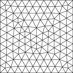
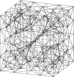
Figure 1. 2d triangular partition with $h=1/10$ (left) / 3d tetrahedral partition with $h=1/4$ (right).

We solve the quad-curl problem on a sequence of meshes with $h=1/10,1/20,1/40,1/80$. The convergence histories under the $\|\cdot\|_{\mathrm{DG}}$ and $\|\cdot\|_{L^{2}(\Omega)}$ are shown in Fig. 2. We observe the optimal convergence of DG norm and suboptimal convergence of $L^{2}$ norm.

$m$	2	3	4
$\eta$	30	30	30
$\#S$	12	20	25

$m$	2	3
$\eta$	40	40
$\#S$	20	40

Table 1. The $\#S$ used in 2D and 3D examples.

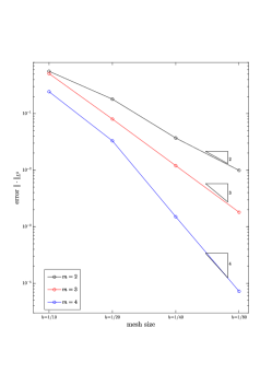
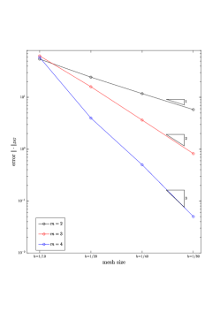
Figure 2. The convergence histories under the $\|\cdot\|_{L^{2}(\Omega)}$ (left) and the$\|\cdot\|_{\mathrm{DG}}$ (right) in Example 1.

Example 2. Here we solve a 3D problem on $\Omega=(0,1)^{3}$. We select the exact solution as

$$\boldsymbol{u}(x,y,z)=\begin{bmatrix}\sin(\pi y)\sin(\pi z)\\ \sin(\pi z)\sin(\pi x)\\ \sin(\pi x)\sin(\pi y)\\ \end{bmatrix},$$

We discretize the problem on successively refined meshes with $h=1/4,1/8,1/16$. The convergence order is shown in Fig. 3, which confirms our theoretical result.

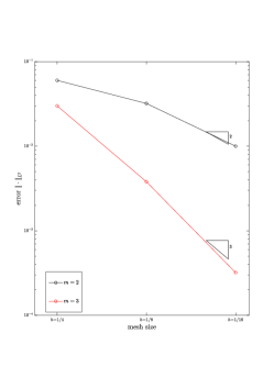
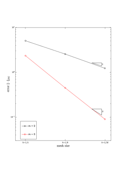
Figure 3. The convergence histories under the $\|\cdot\|_{L^{2}(\Omega)}$ (left) and the $\|\cdot\|_{\mathrm{DG}}$(right) in Example 2.

6. Conclusion

In this paper, we introduce an arbitrary order discontinuous Galerkin finite element method to address the quad-curl problem. The discretization is based on a mixed method approach. The approximation space is built using a patch reconstruction operator, ensuring that the number of degrees of freedom remains unaffected by the approximation order. We establish optimal convergence in the energy norm and suboptimal convergence in the $L^{2}$ norm. Furthermore, we conduct numerical experiments in both two and three dimensions to validate our theoretical findings.

References

- [1] N. Ben Salah, A. Soulaimani, and W. G. Habashi, A finite element method for magnetohydrodynamics, Comput. Methods Appl. Mech. Engrg. 190 (2001), no. 43-44, 5867–5892. MR 1848902
- [2] S. C. Brenner and L. R. Scott, The Mathematical Theory of Finite Element Methods, third ed., Texts in Applied Mathematics, vol. 15, Springer, New York, 2008.
- [3] F. Cakoni, D. Colton, P. Monk, and J. Sun, The inverse electromagnetic scattering problem for anisotropic media, Inverse Problems 26 (2010), no. 7, 074004, 14. MR 2644031
- [4] F. Cakoni and H. Haddar, A variational approach for the solution of the electromagnetic interior transmission problem for anisotropic media, Inverse Probl. Imaging 1 (2007), no. 3, 443–456. MR 2308973
- [5] C. Geuzaine and J. F. Remacle, Gmsh: A 3-D finite element mesh generator with built-in pre- and post-processing facilities, Internat. J. Numer. Methods Engrg. 79 (2009), no. 11, 1309–1331.
- [6] J.-L. Guermond, R. Laguerre, J. Léorat, and C. Nore, An interior penalty Galerkin method for the MHD equations in heterogeneous domains, J. Comput. Phys. 221 (2007), no. 1, 349–369. MR 2290574
- [7] J. Han and Z. Zhang, An -version interior penalty discontinuous Galerkin method for the quad-curl eigenvalue problem, BIT 63 (2023), no. 4, Paper No. 56, 29. MR 4666352
- [8] Jiayu Han and Zhimin Zhang, An hp-version interior penalty discontinuous galerkin method for the quad-curl eigenvalue problem, BIT Numerical Mathematics 63 (2023), article number 56.
- [9] Q. Hong, J. Hu, S. Shu, and J. Xu, A discontinuous Galerkin method for the fourth-order curl problem, J. Comput. Math. 30 (2012), no. 6, 565–578. MR 3041683
- [10] K. Hu, Q. Zhang, and Z. Zhang, Simple curl-curl-conforming finite elements in two dimensions, SIAM J. Sci. Comput. 42 (2020), no. 6, A3859–A3877. MR 4186537
- [11] R. Li, Q. Liu, and F. Yang, A reconstructed discontinuous approximation on unfitted meshes to and interface problems, Comput. Methods Appl. Mech. Engrg. 403 (2023), no. part A, Paper No. 115723, 27.
- [12] R. Li, P. Ming, Z. Sun, and Z. Yang, An arbitrary-order discontinuous Galerkin method with one unknown per element, J. Sci. Comput. 80 (2019), no. 1, 268–288.
- [13] R. Li, P. Ming, and F. Tang, An efficient high order heterogeneous multiscale method for elliptic problems, Multiscale Model. Simul. 10 (2012), no. 1, 259–283.
- [14] R. Li and F. Yang, A reconstructed discontinuous approximation to Monge-Ampère equation in least square formulation, Adv. Appl. Math. Mech. 15 (2023), no. 5, 1109–1141. MR 4613677
- [15] P. Monk, Finite element methods for Maxwell’s equations, Numerical Mathematics and Scientific Computation, Oxford University Press, New York, 2003.
- [16] P. Monk and J. Sun, Finite element methods for Maxwell’s transmission eigenvalues, SIAM J. Sci. Comput. 34 (2012), no. 3, B247–B264. MR 2970278
- [17] M. J. D. Powell, Approximation theory and methods, Cambridge University Press, Cambridge-New York, 1981.
- [18] J. Sun, A mixed FEM for the quad-curl eigenvalue problem, Numer. Math. 132 (2016), no. 1, 185–200. MR 3439219
- [19] C. Wang, Z. Sun, and J. Cui, A new error analysis of a mixed finite element method for the quad-curl problem, Appl. Math. Comput. 349 (2019), 23–38. MR 3894188
- [20] Chunmei Wang, Wang Junping, and Shangyou Zhang, Weak galerkin finite element methods for quad-curl problems, Journal of Computational and Applied Mathematics 428 (2023), 115186.
- [21] Q. Zhang, L. Wang, and Z. Zhang, -conforming finite elements in 2 dimensions and applications to the quad-curl problem, SIAM J. Sci. Comput. 41 (2019), no. 3, A1527–A1547. MR 3949709
- [22] Qian Zhang, A family of curl-curl conforming finite elements on tetrahedral meshes, CSIAM Transactions on Applied Mathematics 1 (2020), 639–663.
- [23] S. Zhang, Mixed schemes for quad-curl equations, ESAIM Math. Model. Numer. Anal. 52 (2018), no. 1, 147–161. MR 3808156
- [24] B. Zheng, Q. Hu, and J. Xu, A nonconforming finite element method for fourth order curl equations in , Math. Comp. 80 (2011), no. 276, 1871–1886. MR 2813342
- [25] Jiguang Sun, Qian Zhang, and Zhimin Zhang, A curl-conforming weak galerkin method for the quad-curl problem, BIT Numerical Mathematics 59 (2019).