Nonlinear Langevin functionals for a driven probe

Abstract

When a probe particle immersed in a fluid with nonlinear interactions is subject to strong driving, the cumulants of the stochastic force acting on the probe are nonlinear functionals of the driving protocol. We present a Volterra series for these nonlinear functionals, by applying nonlinear response theory in a path integral formalism, where the emerging kernels are shown to be expressed in terms of connected equilibrium correlation functions. The first cumulant is the mean force, the second cumulant characterizes the non-equilibrium force fluctuations (noise), and higher order cumulants quantify non-Gaussian fluctuations. We discuss the interpretation of this formalism in relation to Langevin dynamics. We highlight two example scenarios of this formalism: i) For a particle driven with prescribed trajectory, the formalism yields the non-equilibrium statistics of the interaction force with the fluid. ii) For a particle confined in a moving trapping potential, the formalism yields the non-equilibrium statistics of the trapping force. In simulations of a model of nonlinearly interacting Brownian particles, we find that nonlinear phenomena, such as shear-thinning and oscillating noise covariance, appear in third or second order response, respectively.

I Introduction

The jittery motion of a Brownian particle in a Newtonian fluid is well described by a Markovian Langevin equation, since the time scales of the relaxation of the solvent and that of a Brownian particle are separated [1]. More complex fluids, such as colloidal suspensions, polymer solutions or others, can, in contrast, exhibit structural relaxation times on the order of seconds or longer [1, 2, 3]. Brownian particles in such surroundings thus experience memory, and a non-Markovian description is required, achieved, e.g., via projection operator techniques [4, 5, 6, 7], in which a set of degrees of freedom are projected out. For linear systems, such as the famous Caldeira-Leggett model [8, 6], using a bath of harmonic oscillators, such techniques can be applied explicitly to obtain exact non-Markovian Langevin equations. Projection-operator techniques have also been applied in mode-coupling theory (MCT) [9, 10], including predictions of the sub-diffusive plateau in mean squared displacements [11] observed experimentally [12, 13, 14, 15].

Going beyond equilibrium and harmonic cases, i.e., by considering a driven probe particle surrounded by fluid particles with anharmonic interactions, the probe will excite the bath (the fluid particles) out of equilibrium, such that the probe may in general be expected to be subject to non-equilibrium, non-Markovian, and non-Gaussian forces and noise. This can manifest itself, for example, in particle oscillations [16, 17], shear-thinning [18, 19, 20] observed in experiments with micellar fluids [21, 22, 23, 24], superdiffusive behavior [20, 25, 26] or effective temperature [27, 28, 29, 30].

Theoretical description of nonlinear stochastic dynamics of a driven probe is challenging, both conceptually as well as practically, and subject of intense research in recent years. The mentioned projection operator techniques have been extended to nonlinear and non-equilibrium cases [31, 32, 19, 33, 34, 35, 36, 37, 38, 39, 40, 41]; field theory approaches [28, 17], dynamical density functional theory [42, 43, 44, 45, 46, 47, 40], lattice models [26] and nonlinear response theory [48, 49, 50] within path integral formalism [51, 52, 53] have been applied.

In this manuscript, we present a formalism, based on the methods developed in Refs. 49, 50, for systematic expansion of the force cumulants experienced by a probe driven in a fluid of nonlinearly interacting Brownian particles. We therefore derive Volterra series for these cumulants, and find explicit expressions for the respective kernels. Notably, it is the connected equilibrium correlation functions that appear in these kernels. We interpret the resulting Langevin functionals in relation to Langevin dynamics. We evaluate the kernels in a specific nonlinear model, the stochastic Prandtl-Tomlinson model [54, 24, 55], and discuss two different driving modes.

This paper is organized as follows: we start with an explanation of the setup in Sec. II. In Sec. III we move to a path integral representation and present the expansion scheme. We derive the Volterra series for the nonlinear Langevin functionals, the interpretation of which we discuss in Sec. IV. In Sec. V we discuss the application to a specific system, the stochastic Prandtl-Tomlinson model and confirm theoretical predictions with simulations of steady velocity driving in two scenarios of direct and indirect driving.

II Setup

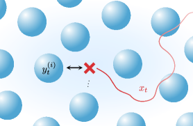
Figure 1: Setup of $N$ Brownian overdamped degrees of freedom (blue) and one external control parameter $x_{t}$ (red). The $i$-th Brownian degree of freedom $y^{(i)}$ experiences a potential gradient $-\partial_{y^{(i)}}U(\{y^{(i)}-x\})$ that can encompass pairwise interactions and coupling to the control parameter.

We consider $N$ Brownian, overdamped degrees of freedom y, with $y^{(i)}$, $i=1\dots N$, the $i$th component, see Fig. 1. These are subject to a potential $U(\{y^{(i)}_{t}-x_{t}\})$, which encompasses mutual interactions between the Brownian degrees as well as interactions with an external control parameter $x_{t}$, with time index $t$: $x_{t}$ is deterministic, and it takes the role of the time-dependent perturbation that is applied to the system (the protocol). Degree $i$ is subject to a bare friction coefficient $\gamma_{i}$, so that it follows the equations of motion,

$$\gamma_{i}\dot{y}_{t}^{(i)} =-\partial_{y^{(i)}_{t}}U(\{y^{(i)}_{t}-x_{t}\})+\xi_{t}^{(i)}$$ (1)

with Gaussian white noise $\xi_{t}^{(i)}$,

$$\left\langle\xi_{t}^{(i)}\right\rangle=0\quad\text{and}\quad\left\langle\xi_{t}^{(i)}\xi_{t^{\prime}}^{(j)}\right\rangle=2k_{B}T\gamma_{i}\delta_{ij}\delta(t-t^{\prime}).$$ (2)

The observable of our interest is $\partial_{x}U(\{y^{(i)}-x\})$, i.e., (minus) the stochastic force that acts on the controlled parameter $x$ . We will find a Volterra series for its cumulants. This setup encompasses, among others, the following two explicit cases. In example (i) $x$ parametrises the position of a trapping potential that acts on one of the particles, say particle 1 [27, 23, 24]. In this case, $\partial_{x}U(\{y^{(i)}-x\})$ is the force acting on this particle by the trapping potential, accessible in experiments [27, 23, 24]. In example (ii), $x$ is the position of a probe particle that is driven with controlled velocity. In this case, $\partial_{x}U(\{y^{(i)}-x\})$ is (minus) the stochastic force the driven particle feels from the Brownian degrees of freedom, i.e., the resulting ”frictional force“. This case may be accessible in experiments with feedback control [57].

We note that the observable of interest, $\partial_{x_{t}}U(\{y^{(i)}_{t}-x_{t}\})$, depends explicitly on time, via $x_{t}$. This makes a perturbative expansion of it in powers of displacements of $x_{t}$ cumbersome [52, 53, 50], because the expansion also includes explicit expansion of the observable. Identifying entropy production (see below) appears also nontrivial in this case [53, 58]. It is thus beneficial to introduce relative coordinates $q^{(i)}=y^{(i)}-x$ and to transform to a frame comoving with $x_{t}$. In this frame, the $q^{(i)}$ follow

$$\gamma_{i}\dot{q}_{t}^{(i)} =-\gamma_{i}\dot{x}_{t}-\partial_{q^{(i)}_{t}}U(\mathbf{q}_{t})+\xi_{t}^{(i)}.$$ (3)

We note that the simple transformation of Eq. (1) to the moving frame is the main reason to restrict to overdamped, Brownian degrees of freedom.

Using translational invariance of the potential $U$, the observable $\partial_{x_{t}}U(\{y_{t}^{(i)}-x_{t}\})$ reads in these coordinates

$$\begin{split}F_{t}&\equiv\partial_{x_{t}}U(\{y_{t}^{(i)}-x_{t}\})=-\sum_{i}\partial_{y^{(i)}_{t}}U(\{y^{(i)}_{t}-x_{t}\})\\ &=-\sum_{i}\partial_{q^{(i)}_{t}}U(\mathbf{q}_{t}).\end{split}$$ (4)

The explicit dependence on time $t$ thus disappeared in this frame, easing the expansion.

III Volterra Series

We aim to expand the cumulants of the force $\partial_{x_{t}}U(\{y_{t}^{(i)}-x_{t}\})=F(\textbf{q}_{t})\equiv F_{t}$ in a Volterra series in the driving by applying a path integral formalism [52, 53]. Therefore consider paths $\omega=(\textbf{q}_{s},t_{0}\leq s\leq t)$ of the $N$ Brownian degrees of freedom over a time-interval $[t_{0},t]$ with $\textbf{q}_{s}$ the state of $N$ Brownian degrees of freedom at time $s$, prepared, at $t_{0}$, in the equilibrium distribution corresponding to $x$ at rest at $x_{t_{0}}$. The expectation value of observable $O(\omega)$ under the protocol $\scaleobj{.65}{{\mathcal{X}}}=(x_{s},t_{0}\leq s\leq t)$ is given by the path integral

$$\langle O(\omega)\rangle=\int\mathcal{D}\omega\,\mathcal{P}(\scaleobj{.65}{{\mathcal{X}}},\omega)O(\omega),$$ (5)

with $\mathcal{D}\omega$ the path element and $\mathcal{P}(\scaleobj{.65}{{\mathcal{X}}},\omega)$ the path weight, a functional of $\omega$ depending on protocol $\scaleobj{.65}{{\mathcal{X}}}$. The latter is expressed in terms of the equilibrium path weight $\mathcal{P}_{\mathrm{eq}}$ and perturbation action $\mathcal{A}$,

$$\mathcal{P}(\scaleobj{.65}{{\mathcal{X}}},\omega)=e^{-\mathcal{A}(\scaleobj{.65}{{\mathcal{X}}},\omega)}\mathcal{P}_{\mathrm{eq}}(\omega).$$ (6)

$\mathcal{P}_{\mathrm{eq}}(\omega)$ contains the Boltzmann distribution. The action $\mathcal{A}$ follows from the difference of the Onsager-Machlup action functional [59] corresponding to Eq. (3) for finite and zero velocity of $x$,

$$\begin{split}\mathcal{A}(\scaleobj{.65}{{\mathcal{X}}},\omega)=\sum_{i}\frac{\gamma_{i}}{4k_{B}T}\int_{t_{0}}^{t}\mathrm{d}s\,\Bigg{[}-\left(\dot{q}_{s}^{(i)}+\frac{\partial_{q^{(i)}_{s}}U(\mathbf{q}_{s})}{\gamma_{i}}\right)^{2}&\\ +\left(\dot{q}_{s}^{(i)}+\dot{x}_{s}+\frac{\partial_{q^{(i)}_{s}}U(\mathbf{q}_{s})}{\gamma_{i}}\right)^{2}\Bigg{]}&\end{split}$$ (7)

$$=\frac{1}{2k_{B}T}\int_{t_{0}}^{t}\mathrm{d}s\left[-\dot{x}_{s}F_{s}+\sum_{i}\frac{\gamma_{i}}{2}\left(2\dot{x}_{s}\dot{q}_{s}^{(i)}+\dot{x}_{s}^{2}\right)\right]$$ . (8)

Eq. (8) contains the driving $\dot{x}$ up to second order for the model of Brownian degrees. It is insightful to decompose $\mathcal{A}$ into its time-antisymmetric part $S(\omega)$, termed the entropic component, and its time-symmetric part $D(\omega)$. The latter, named frenetic part [60], has no thermodynamic meaning, and we refer to it as non-thermodynamic (NT) component in the following: $\mathcal{A}\coloneqq D-S/2$ [61, 51, 60, 52, 53, 58, 50]. $S(\theta\omega)=-S(\omega)$ and $D(\theta\omega)=D(\omega)$, with time reversal operator $\theta$, i.e., $(\theta\scaleobj{.65}{{\mathcal{X}}},\theta\omega)_{s}=\pi(x_{t-s},\mathbf{q}_{t-s})$ with $\pi$ denoting the kinematical time-reversal. Taking into account the change of sign of velocities under time reversal, we can read off the respective entropic and NT components (denoting by ^′ and ^′′ the terms in first and second order of driving, respectively),

$$S=S^{\prime} =\frac{1}{k_{B}T}\int_{t_{0}}^{t}\mathrm{d}s\,\dot{x}_{s}F_{s}$$ (9)

$$D^{\prime} =\sum_{i}\frac{\gamma_{i}}{2k_{B}T}\int_{t_{0}}^{t}\mathrm{d}s\,\dot{x}_{s}\dot{q}_{s}^{(i)}$$ (10)

$$D^{\prime\prime} =\frac{\sum_{i}\gamma_{i}}{2k_{B}T}\int_{t_{0}}^{t}\mathrm{d}s\int_{t_{0}}^{t}\mathrm{d}s^{\prime}\,\dot{x}_{s}\dot{x}_{s^{\prime}}\delta(s-s^{\prime}).$$ (11)

Eq. (9) thus corresponds to the entropy change with respect to the reference equilibrium ensemble, $S=\ln\frac{\mathcal{P}(\scaleobj{.65}{{\mathcal{X}}},\omega)}{\mathcal{P}(\theta\scaleobj{.65}{{\mathcal{X}}},\theta\omega)}$ [53, 62]. It is inherently linear in the perturbation, $S=S^{\prime}$, which also appears to be specific for the Brownian system [53]. For the NT components, Eqs. (10) and (11), we introduce abbreviations $\mathcal{D}_{s}\coloneqq\sum_{i}\frac{\gamma_{i}}{2k_{B}T}\dot{q}_{s}^{(i)}$ and $\mathcal{D}_{s,s^{\prime}}\coloneqq\frac{\sum_{i}\gamma_{i}}{2k_{B}T}\delta(s-s^{\prime})$, i.e.,

$$D^{\prime} =\int_{t_{0}}^{t}\mathrm{d}s\,\dot{x}_{s}\mathcal{D}_{s}$$ (12)

$$D^{\prime\prime} =\int_{t_{0}}^{t}\mathrm{d}s\int_{t_{0}}^{t}\mathrm{d}s^{\prime}\,\dot{x}_{x}\dot{x}_{s^{\prime}}\mathcal{D}_{s,s^{\prime}}.$$ (13)

Expanding also the exponential in Eq. (6), the response for any path observable $O=O(\omega)$ is given by [51, 52, 53]

$$\begin{split}\langle O\rangle&=\langle O\rangle_{\mathrm{eq}}-\langle(D^{\prime}-S^{\prime}/2)O\rangle_{\mathrm{eq}}\\ &\quad+\frac{1}{2}\langle(D^{\prime 2}-D^{\prime\prime}-D^{\prime}S^{\prime}+S^{\prime 2}/4)O\rangle_{\mathrm{eq}}+\dots\end{split}$$ (14)

While Eq. (14) holds for path observables, considering state observables $O_{t}\coloneqq O(\mathbf{q}_{t})$ allows for simplifications: taking the difference $\langle O_{t}\rangle-\langle O(\theta\omega)\rangle$ yields, because of initial preparation in equilibrium [52, 53, 50]

$$\begin{split}&\langle O_{t}\rangle-\langle O_{t}\rangle_{\mathrm{eq}}=\langle S^{\prime}O_{t}\rangle_{\mathrm{eq}}-\langle D^{\prime}S^{\prime}O_{t}\rangle_{\mathrm{eq}}\\ &\quad+\frac{1}{6}\left\langle\left[3D^{\prime 2}-3D^{\prime\prime}+\frac{S^{\prime 2}}{4}\right]S^{\prime}O_{t}\right\rangle_{\mathrm{eq}}+\dots\end{split}$$ (15)

See Eq. (49) in Appendix B [63] for the higher order terms of Eq. (15), which, for any order $n$, can be given in closed form.

Notably, the terms shown in Eq. (15) may individually diverge for large $t$ for specific cases, see discussion in Appendix C. We can however show that these divergences analytically cancel, and that Eq. (15) can be expressed in terms of connected correlation functions $\langle\cdot;\dots;\cdot\rangle$, which are mathematically equivalent to joint cumulants (see Appendix A for the definition), i.e.

$$\begin{split}\langle O_{t}\rangle-\langle O_{t}\rangle_{\mathrm{eq}}&=\langle S^{\prime};O_{t}\rangle_{\mathrm{eq}}-\langle D^{\prime};S^{\prime};O_{t}\rangle_{\mathrm{eq}}\\ &\quad+\frac{1}{2}\left[\langle D^{\prime};D^{\prime};S^{\prime};O_{t}\rangle_{\mathrm{eq}}-\langle D^{\prime\prime};S^{\prime};O_{t}\rangle_{\mathrm{eq}}\right]\\ &\quad+\frac{1}{24}\langle S^{\prime};S^{\prime};S^{\prime};O_{t}\rangle_{\mathrm{eq}}+\dots\end{split}$$ (16)

Note that we have only shown this up to including third order, and we do not know whether the higher order terms can be written in terms of connected correlation functions as well. For the derivation we refer to Appendix A.

The notion of connected correlation functions is reminiscent of connected Feynman diagrams in field theoretic approaches [64]. It will be worth exploring this connection in future work. We illustrate the resulting cancellations in Appendix C for the specific example discussed in Sec. V.3.

The occurrence of connected correlations is not restricted to state observables. For path observables $O(\omega)$ we can equally express the response (here proven up to second order)

$$\begin{split}&\langle O\rangle-\langle O\rangle_{\mathrm{eq}}=\left[\frac{1}{2}\langle S^{\prime};O\rangle_{\mathrm{eq}}-\langle D^{\prime};O\rangle_{\mathrm{eq}}\right]-\frac{1}{2}\langle D^{\prime\prime};O\rangle_{\mathrm{eq}}\\ &+\frac{1}{2}\Big{[}\langle D^{\prime};D^{\prime};O\rangle_{\mathrm{eq}}-\langle D^{\prime};S^{\prime};O\rangle_{\mathrm{eq}}+\frac{1}{4}\langle S^{\prime};S^{\prime};O\rangle_{\mathrm{eq}}\Big{]}+\dots\end{split}$$ (17)

It is also worth noting that all response relations presented in this section are independent of the assumption of Brownian overdamped degrees of freedom. Mathematically, they are solely based on the expansion $\mathcal{A}=D^{\prime}-S^{\prime}/2+D^{\prime\prime}/2+\dots$. To our knowledge Eqs. (16) and (17) have not been given in literature.

In the following, we will apply Eqs. (16), (17), and (9)-(11) to find the cumulants of the stochastic force $F_{t}$. Eq. (16) is used to obtain the mean force $\langle F_{t}\rangle$, while higher cumulants $\langle F_{t};F_{t^{\prime}}\rangle$, $\langle F_{t};F_{t^{\prime}};F_{t^{\prime\prime}}\rangle,\dots$ follow from Eq. (17). We formally take the limit $t_{0}\to-\infty$ in Eqs. (9)-(11) to allow for arbitrary driving protocols $\dot{x}_{t}$. For example, steady-state averages follow then with a time independent driving velocity, and transient ones are obtained by use of a step function $\dot{x}_{t}\propto\Theta(t)$. Noting that the mean force vanishes for the equilibrium case, the resulting Volterra series take on the form (with $\beta=(k_{B}T)^{-1}$)

$$\beta\langle F_{t}\rangle =\int_{-\infty}^{t}\mathrm{d}s\,\dot{x}_{s}\Gamma_{t-s}^{(0,1)}+\int_{-\infty}^{t}\mathrm{d}s\int_{-\infty}^{t}\mathrm{d}s^{\prime}\,\dot{x}_{s}\dot{x}_{s^{\prime}}\Gamma_{t-s,t-s^{\prime}}^{(0,2)}+\int_{-\infty}^{t}\mathrm{d}s\int_{-\infty}^{t}\mathrm{d}s^{\prime}\int_{-\infty}^{t}\mathrm{d}s^{\prime\prime}\,\dot{x}_{s}\dot{x}_{s^{\prime}}\dot{x}_{s^{\prime\prime}}\Gamma_{t-s,t-s^{\prime},t-s^{\prime\prime}}^{(0,3)}+\dots$$ (18)

$$\beta^{2}\langle F_{t};F_{t^{\prime}}\rangle =\Gamma_{t-t^{\prime}}^{(1,0)}+\int_{-\infty}^{t}\mathrm{d}s\,\dot{x}_{s}\Gamma^{(1,1)}_{t-s;t-t^{\prime}}+\int_{-\infty}^{t}\mathrm{d}s\int_{-\infty}^{t}\mathrm{d}s^{\prime}\,\dot{x}_{s}\dot{x}_{s^{\prime}}\Gamma^{(1,2)}_{t-s,t-s^{\prime};t-t^{\prime}}+\dots$$ (19)

$$\beta^{3}\langle F_{t};F_{t^{\prime}};F_{t^{\prime\prime}}\rangle =\Gamma^{(2,0)}_{t-t^{\prime},t-t^{\prime\prime}}+\int_{-\infty}^{t}\mathrm{d}s\,\dot{x}_{s}\Gamma^{(2,1)}_{t-s;t-t^{\prime},t-t^{\prime\prime}}+\dots$$ (20)

$$\;\;\vdots$$

Here we have assumed the existence of response kernels $\Gamma^{(m,n)}$, with $m+1$ and $n$ indicating the order of cumulant and order of perturbation, respectively. The forms (18) - (20) and higher orders are so far pure definitions, not related to the system at hand,

$$\begin{split}\Gamma^{(m,n)}&{}_{t-s_{1},\dots,t-s_{n};t-t_{1},\dots,t-t_{m}}\\ &\coloneqq\frac{\beta^{m+1}}{n!}\frac{\delta^{n}}{\delta\dot{x}_{s_{1}}\cdots\delta\dot{x}_{s_{n}}}\langle F_{t};F_{t_{1}};\dots;F_{t_{m}}\rangle\Big{|}_{\{\dot{x}\}=0}.\end{split}$$ (21)

The novelty of this manuscript is now contained in obtaining these kernels in terms of correlation functions. These follow from the above laid out expansion. Explicitly, the leading order kernels for the mean force, i.e., $m=0$, read

$$\Gamma_{s}^{(0,1)} =\beta^{2}\langle F_{s};F_{0}\rangle_{\mathrm{eq}},$$ (22)

$$\Gamma_{s,s^{\prime}}^{(0,2)} =\frac{\beta^{2}}{2}\left(\left\langle\mathcal{D}_{s};F_{s^{\prime}};F_{0}\right\rangle_{\mathrm{eq}}+\langle\mathcal{D}_{s^{\prime}};F_{s};F_{0}\rangle_{\mathrm{eq}}\right),$$ (23)

$$\begin{split}\Gamma_{s_{1},s_{2},s_{3}}^{(0,3)}&=\frac{1}{6}\sum_{\pi\in S_{3}}\Bigg{(}\frac{\beta^{2}}{2}\Big{[}\left\langle\mathcal{D}_{s_{\pi(1)}};\mathcal{D}_{s_{\pi(2)}};F_{s_{\pi(3)}};F_{0}\right\rangle_{\mathrm{eq}}\\ &\quad\quad\quad\quad\quad\quad-\left\langle\mathcal{D}_{s_{\pi(1)},s_{\pi(2)}};F_{s_{\pi(3)}};F_{0}\right\rangle_{\mathrm{eq}}\Big{]}\\ &\quad\quad\quad\quad+\frac{\beta^{4}}{24}\langle F_{s_{\pi(1)}};F_{s_{\pi(2)}};F_{s_{\pi(3)}};F_{0}\rangle_{\mathrm{eq}}\Bigg{)},\end{split}$$ (24)

$$\;\;\vdots$$

where the sum in $\Gamma^{(0,3)}$ goes over all elements of the permutation group $S_{3}$. The first kernels entering the force covariance $\langle F_{t};F_{t^{\prime}}\rangle$, i.e., $m=1$ are given by

$$\Gamma^{(1,0)}_{t-t^{\prime}} =\beta^{2}\langle F_{t-t^{\prime}};F_{0}\rangle_{\mathrm{eq}},$$ (25)

$$\Gamma^{(1,1)}_{s;t-t^{\prime}} =\beta^{2}\left\langle\left(\mathcal{D}_{s}+\frac{\beta F_{s}}{2}\right);F_{t-t^{\prime}};F_{0}\right\rangle_{\mathrm{eq}},$$ (26)

$$\begin{split}\Gamma^{(1,2)}_{s_{1},s_{2};t-t^{\prime}}&=\frac{\beta^{2}}{4}\sum_{\pi\in S_{2}}\Bigg{[}\langle\mathcal{D}_{s_{\pi(1)}};\mathcal{D}_{s_{\pi(2)}};F_{t-t^{\prime}};F_{0}\rangle_{\mathrm{eq}}\\ &\quad\quad\quad\quad-\langle\mathcal{D}_{s_{\pi(1)},s_{\pi(2)}};F_{t-t^{\prime}};F_{0}\rangle_{\mathrm{eq}}\\ &\quad\quad\quad\quad+\beta\langle\mathcal{D}_{s_{\pi(1)}};F_{s_{\pi(2)}};F_{t-t^{\prime}};F_{0}\rangle_{\mathrm{eq}}\\ &\quad\quad\quad\quad+\frac{\beta^{2}}{4}\langle F_{s_{\pi(1)}};F_{s_{\pi(2)}};F_{t-t^{\prime}};F_{0}\rangle_{\mathrm{eq}}\Bigg{]}.\end{split}$$ (27)

$$\;\;\vdots$$

These thus quantify how the force covariance changes due to the driving. The kernels for the third cumulant $\langle F_{t};F_{t^{\prime}};F_{t^{\prime\prime}}\rangle$ ($m=2$) read

$$\Gamma^{(2,0)}_{t-t^{\prime},t-t^{\prime\prime}} =\beta^{3}\langle F_{t-t^{\prime}};F_{t-t^{\prime\prime}};F_{0}\rangle_{\mathrm{eq}},$$ (28)

$$\Gamma^{(2,1)}_{s;t-t^{\prime},t-t^{\prime\prime}} =\beta^{3}\left\langle\left(\mathcal{D}_{s}+\frac{\beta F_{s}}{2}\right);F_{t-t^{\prime}};F_{t-t^{\prime\prime}};F_{0}\right\rangle_{\mathrm{eq}}.$$ (29)

$$\;\;\vdots$$

The kernels with $m=2$ are thus the leading measure how non-Gaussianity occurs due to, or is affected by driving.

Due to the determinacy of the protocol $\dot{x}_{t}$, $x_{t}$ can be moved out of averages, and the kernels only contain forces $F_{s}$ and NT coefficients $\mathcal{D}_{s}$, $\mathcal{D}_{s,s^{\prime}}$. We have applied time-reversal symmetry and stationarity of equilibrium correlation functions, thereby finding that all kernels $\Gamma^{(m,n)}_{t-s_{1},\dots,t-s_{n};t-t_{1},\dots,t-t_{m}}$ only depend on time differences $t-s_{1}$, $t-s_{2}$, …, as already assumed in Eqs. (18) - (20). From the definition, Eq. (21), it becomes clear that the kernels are separately symmetric under exchange of the time arguments within one block, i.e. under changes of time arguments $s_{1},\dots,s_{n}$ and, separately, under changes of time arguments $t_{1},\dots,t_{m}$. The symmetry with respect to changes of time arguments $s_{i}$ is enforced by hand, namely through the sums over all elements of respective permutation groups in Eqs. (22)-(29). We note that Eqs. (25) and Eqs. (22) display the equality $\Gamma^{(0,1)}=\Gamma^{(1,0)}$, which is the fluctuation dissipation theorem.

We derive a general expression for the $n-$th order memory kernel $\Gamma^{(0,n)}$ in Appendix B. This expression uses Eq. (15), i.e., it is not given in terms of connected correlation functions. We thus provide a framework to study non-Gaussian fluctuations in non-equilibrium.

IV Interpretation of nonlinear Langevin functionals

We have in the introduction mentioned that nonlinear stochastic motion is conceptually and practically challenging, with intense efforts and developments [38, 39, 35, 36, 37, 41].

How are Eqs. (18)-(21) interpreted? These are the non-equilibrium force cumulants, which characterize the non-Gaussian, non-equilibrium statistics of the force acting on an externally driven control parameter $x_{t}$. This is relevant and experimentally observable, for example via a Brownian particle confined in a moving trapping potential [27, 23, 24].

It is however important to keep in mind that $\dot{x}$ appearing in Eqs. (18)-(21) is the deterministic velocity of the control parameter. Our formulation is thus nonlinear in this control parameter. It is not a nonlinear equation for a stochastic degree of freedom. This formulation is thus, a priori, not an equation of motion of a Brownian particle. It may however, in certain scenarios or limits, for example the Markovian limit, turn into a nonlinear equation for a stochastic degree. This is not known to us and needs to be investigated in future work.

What we derive here is thus not a Langevin equation, and we refer to Eqs. (18)-(20) as nonlinear Langevin functionals.

V Driving in the stochastic Prandtl-Tomlinson model

V.1 Introduction and protocol

In this section we will discuss simulation results for a specific system of Brownian overdamped degrees of freedom, the so-called stochastic Prandtl-Tomlinson model [54, 24, 55]. In previous works, this model was shown to contain several nonlinear phenomena experimentally observed in viscoelastic systems such as shear-thinning, particle oscillations [24] and a trap stiffness dependent memory kernel [54]. We will study the nonlinear force functionals for two driving modes: direct and indirect driving. These correspond to two different controlled degrees of freedom as will be detailed below.

We restrict to steady driving velocity, i.e., a protocol of

$$\dot{x}_{t}=v\Theta(t-t_{0}),$$ (30)

and we denote the corresponding averages by $\langle\dots\rangle^{(-t_{0})}$. Using $t_{0}=0$ and $t_{0}\to-\infty$ yields transient and steady state averages, respectively.

V.2 Model and driving modes

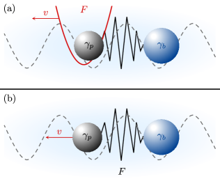
Figure 2: Sketch of the Stochastic Prandtl-Tomlinson model: a probe particle (gray) with friction coefficient $\gamma_{p}$ is coupled to a bath particle (blue) with friction coefficient $\gamma_{b}$ via a sinusoidal interaction potential (dashed line). The upper panel (a) highlights the scenario of indirect driving, in which the probe is confined in a harmonic trapping potential (red), i.e. experiences a trapping force $F$. The center of the trapping potential is driven with velocity $v$. The lower panel (b) shows the scenario of direct driving in which the position of the probe particle corresponds to the protocol, hence follows a given velocity $v$. In this scenario, the force $F$ of the laid out formalism is the interaction force between probe and bath.

Consider two coupled Brownian particles: one probe particle at position $y^{(p)}$ and one bath particle at position $y^{(b)}$. Each of the particles is characterized by a friction coefficient $\gamma_{p}$ or $\gamma_{b}$, respectively. The two particles interact via a sinusoidal potential [54]

$$U_{\mathrm{int}}\left(y^{(b)}-y^{(p)}\right)=-U_{0}\cos\left(\frac{2\pi}{d}\left(y^{(b)}-y^{(p)}\right)\right)$$ (31)

with amplitude $U_{0}$ and length scale $d$, see dashed line in Fig. 2. The interaction potential is thus a non-binding potential, such that probe and bath particle can move with different (mean) velocities, when the probe is driven [54]. This is for example required to observe shear-thinning [55, 24]. This model was termed stochastic Prandtl-Tomlinson model [54].

In indirect driving, the probe particle is confined in a trapping potential, whose center is the controlled parameter $x_{t}$, see Fig. 2(a). In this mode, $y^{(1)}=y^{(p)}$ and $y^{(2)}=y^{(b)}$ are the two Brownian overdamped degrees of freedom with $\gamma_{1}=\gamma_{p}$ and $\gamma_{2}=\gamma_{b}$ that obey Eq. (1). Here, we choose a harmonic trapping potential $U_{\mathrm{ext}}\left(y^{(1)}-x\right)=\frac{1}{2}\kappa\left(y^{(1)}-x\right)^{2}$. In direct driving, the position of the probe particle is deterministic and follows the protocol, i.e. $y^{(p)}=x$ (Fig. 2(b)). In this driving mode we have one Brownian overdamped degree of freedom, the position of the bath particle, i.e. $y^{(1)}=y^{(b)}$ and $\gamma_{1}=\gamma_{b}$.

The two driving modes correspond to the following potential $U=U(\{y^{(i)}-x\})$ in Eq. (1),

$$U=\begin{cases}U_{\mathrm{int}}\left(y^{(2)}-y^{(1)}\right)+U_{\mathrm{ext}}\left(y^{(1)}-x\right),&\text{indirect}\\ U_{\mathrm{int}}\left(y^{(1)}-x\right),&\text{direct}.\end{cases}$$ (32)

The resulting force $F_{t}=\partial_{x_{t}}U(\{y^{(i)}_{t}-x_{t}\})$ reads in the two cases

$$F_{t}=\begin{cases}-\kappa q_{t}^{(1)},&\text{indirect driving}\\ -\frac{2\pi}{d}U_{0}\sin\left(\frac{2\pi}{d}q_{t}^{(1)}\right),&\text{direct driving},\end{cases}$$ (33)

expressed in terms of the relative coordinates $q^{(i)}=y^{(i)}-x$. We follow the protocol in Eq. (30), and we fix the choices $\gamma_{b}=10\,\gamma_{p}$ and $U_{0}=2\,k_{B}T$ throughout: Using $\gamma_{b}$ large compared to $\gamma_{p}$ yields pronounced nonlinear effects. We have found that $U_{0}$ slightly larger than thermal energy is the most interesting regime of the Prandtl Tomlinson model [55]: For $U_{0}\ll k_{B}T$, the effects of the coupling vanish, and for $U_{0}\gg k_{B}T$, the coupling becomes nearly that of a harmonic spring.

V.3 1st Cumulant: Flow Curve

We start by considering the mean force, i.e., we evaluate Eq. (18) in steady state conditions. Dividing the mean force by the driving velocity yields the velocity dependent friction coefficient $\gamma(v)$, or flow curve [24]. For the two scenarios of direct and indirect driving we define [24, 50]

$$\gamma(v)=\frac{\left|\langle F\rangle^{(\infty)}\right|}{v}+\begin{cases}0,&\text{indirect driving}\\ \gamma_{p},&\text{direct driving}.\end{cases}$$ (34)

For a better comparison between the two scenarios we added $\gamma_{p}$ to the case of direct driving in Eq. (34). With this, $\gamma(v)$ of the two cases approach each other for $\kappa\to\infty$, as we shall see below.

From Eq. (18) we find for $\langle F\rangle^{(\infty)}$,

$$\beta\frac{\left|\langle F\rangle^{(\infty)}\right|}{v}=\hat{\Gamma}_{z=0}^{(0,1)}+v^{2}\hat{\Gamma}_{z=0,z=0,z=0}^{(0,3)}+\mathcal{O}(v^{4})$$ (35)

with Laplace transforms defined as $\hat{f}_{z}=\int_{0}^{\infty}\mathrm{d}t\,e^{-zt}f_{t}$; with definitions for multiple time dependencies accordingly. We note that $\Gamma^{(0,2)}$ misses in Eq. (35) as it is zero due to symmetries. The flow curve is an expansion in even powers of $v$.

In Appendix C we discuss in detail how to efficiently compute time-integrated memory kernels, considering the example of $\hat{\Gamma}^{(0,3)}_{z=0,z=0,z=0}$. Moreover, we compare two different ways to do this, based on (i) the ”naive” response relation, Eq. (15), and (ii) the response relation in terms of connected correlation functions, Eq. (16). As mentioned above, connected correlation functions are advantageous as they analytically cancel divergences in individual response terms.

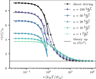
Figure 3: Flow curve $\gamma(v)$ (open symbols with dashed lines) and response curves up to second order according to Eq. (35) (solid lines) for direct driving (black) and indirect driving (colors) with velocity $v$. Different colors correspond to different stiffness $\kappa$ of the harmonic potential.

Fig. 3 shows the resulting comparison of Eq. (34) computed from non-equilibrium simulations (symbols with dashed lines) and response curves up to third order in driving velocity $v$ using equilibrium simulations (according to Eq. (35)). The figure shows flow curves for different stiffness $\kappa$ of the trapping potential (colors) and for direct driving (black). All flow curves exhibit shear-thinning, as extensively discussed for the stochastic Prandtl-Tomlinson model in Refs. 55, 50. We find that shear-thinning, as might be expected, indeed appears in the response curves (solid lines) up to third order. The first-order kernel $\hat{\Gamma}^{(0,1)}_{z=0}$ (with $\gamma_{p}$ added in the direct case) characterizes the plateau $\gamma(v\to 0)$ and increases monotonously with $\kappa$; the probe experiences stronger interaction with the bath particle, if the confinement is strong [54]. The third-order kernel $\hat{\Gamma}_{z=0,z=0,z=0}^{(0,3)}$ characterizes the onset of shear-thinning and shows a non-monotonous behavior in $\kappa$. This is shown in Fig. 7 (discussed in Sec. V.6), displaying that, when the trap stiffness matches the curvature of the interaction potential, nonlinear effects set in most early as a function of $v$.

V.4 2nd Cumulant: Force fluctuations

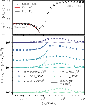
Figure 4: Steady-state force variance as a function of driving velocity for the scenario of direct (top) and indirect (bottom) driving. Open symbols show results from non-equilibrium simulations, the lines correspond to response curves up to $\mathcal{O}(v^{2})$. In the top panel two response curves according to Eq. (19) using Eq. (36) (black dashed line) and Eq. (27) (red line) are shown, demonstrating that they yield identical results as expected. The gray lines depict the limits $v\to 0$ and $v\to\infty$ according to Eqs. (37) and (38). For the scenario of indirect driving the limit of $v\to 0$ given by Eq. (39) is indicated by the colored dotted lines in the bottom panel.

We continue by exploiting Eq. (19) to study the force covariance $\langle F_{t};F_{t^{\prime}}\rangle^{(-t_{0})}$ in various cases, starting with steady-state, i.e., $t_{0}\to-\infty$ and $t=t^{\prime}$. For this case, the second order memory kernel in Eq. (19) can be simplified to

$$\begin{split}\Gamma^{(1,2)}_{s_{1},s_{2};0}=\frac{\beta^{2}}{2}\sum_{\pi\in S_{2}}\left\langle\mathcal{D}_{s_{\pi(1)}};F_{s_{\pi(2)}};F_{0};F_{0}\right\rangle_{\mathrm{eq}},\end{split}$$ (36)

compare Eq. (16). In Fig. 4 we explore the force variance as a function of driving velocity for the two scenarios of direct (top panel) and indirect (lower panel) driving. Open symbols show results from non-equilibrium simulations; lines show response curves up to second order in driving velocity obtained from equilibrium simulations.

In the scenario of direct driving (Fig. 4, top panel) the force variance converges to plateaus in the two limiting cases of $v\to 0$ and $v\to\infty$ and exhibits a minimum in between. The limits $v\to 0$ and $v\to\infty$ can be found analytically, see gray lines in the top panel in Fig. 4. In equilibrium the relative coordinate $q^{(1)}$ between bath and probe particle obeys a Boltzmann distribution with the interaction potential $U_{\mathrm{int}}(q^{(1)})$ (Eq. (31)) which yields

$$\lim_{v\to 0}\langle F_{t};F_{t}\rangle^{(\infty)}=\langle F_{t};F_{t}\rangle_{\mathrm{eq}}=\frac{4\pi^{2}U_{0}I_{1}(\beta U_{0})}{\beta d^{2}I_{0}(\beta U_{0})},$$ (37)

where $I_{n}(z)$ denotes the Bessel function of first kind. In the limit of infinite velocity the distribution of the distance between probe and bath particle can be assumed flat, such that

$$\begin{split}\lim_{v\to\infty}\langle F_{t};F_{t}\rangle^{(\infty)}&=\int_{0}^{d}\mathrm{d}q^{(1)}\left(\frac{2\pi U_{0}}{d}\sin\left(\frac{2\pi}{d}q^{(1)}\right)\right)^{2}\\ &=\frac{2\pi^{2}U_{0}^{2}}{d^{2}},\end{split}$$ (38)

which is also shown in the figure. Notably, $\lim_{v\to\infty}\langle F_{t};F_{t}\rangle^{(\infty)}\geq\langle F_{t};F_{t}\rangle_{\mathrm{eq}}$ for any $\beta U_{0}$, with equality being approached for $\beta U_{0}\to 0$.

The behavior for finite velocity can be understood in the following picture: with increasing driving velocity the probe experiences the anharmonic part of the interaction potential ($\sim-x^{4}$) and the effective curvature decreases, resulting in a decay of the force variance. For larger driving velocities, when shear-thinning takes place, the probe can hop over the barrier and explore the full range of forces, so that the force variance increases. We find that the nonlinear phenomenon of initial decay of the force variance appears in the second-order kernel of the force covariance, $\Gamma^{(1,2)}$. Moreover, we confirm Eq. (36) by comparing response curves using Eq. (36) (dashed black line) and using the original expression, Eq. (27) (red line) in Fig. 4 (top panel).

In the scenario of indirect driving (Fig. 4, bottom panel) we observe a maximum at finite driving velocity for all different values of trap stiffness $\kappa$ (colors). This is feature has been characterized by an increased effective temperature [29, 30, 27]. Also here, the initial increase is captured by the second order memory kernel $\Gamma^{(1,2)}$. The dotted lines in the bottom panel in Fig. 4 correspond to the limit $v\to 0$, found from the Boltzmann distribution with the harmonic trapping potential,

$$\lim_{v\to 0}\langle F_{t};F_{t}\rangle^{(\infty)}=\langle F_{t};F_{t}\rangle_{\mathrm{eq}}=\kappa k_{B}T.$$ (39)

We observe that in the limit of infinite velocity, when probe and bath particle are decoupled, the data points of $\langle F_{t};F_{t}\rangle^{(\infty)}$ appear to approach the dotted line of equilibrium values. This may be understood as the interaction with the bath particle acts as a fixed periodic potential background in this limit. When the probe particle is dragged over this background, the force thus rapidly switches sign and cancels out. Notably, the force fluctuations within the two scenarios are inherently different: in the scenario of direct driving they characterize the interaction between probe and bath out of equilibrium, while they characterize the statistics of the trapping force in the scenario of indirect driving.

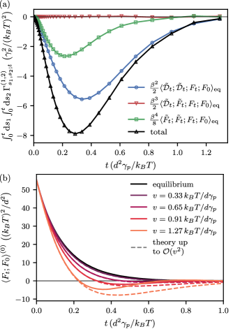
Figure 5: (a) Time-dependence of second order response terms for the transient force covariance in the scenario of direct driving according to Eq. (19). Note that $\tilde{f}_{t}=\int_{0}^{t}\mathrm{d}s\,f_{s}$ is defined as the running integral up to time $t$. (b) Resulting comparison of the transient force covariance (solid lines) with the theoretical response curves up to $\mathcal{O}(v^{2})$ (dashed lines) according to Eq. (19) for several driving velocities in the scenario of direct driving.

Next, we study Eq. (19) for $t^{\prime}=0$ and finite $t$, i.e. consider the transient force covariance $\langle F_{t};F_{0}\rangle^{(0)}$ where the system is prepared in equilibrium at time $t=0$. Therefore, we require the time-dependence of the second-order memory kernel, Eq. (27). The resulting curves for the scenario of direct driving are shown in Fig. 5(a) and exhibit a minimum at short times. Adding the black curve times velocity squared to the equilibrium force covariance $\langle F_{t};F_{0}\rangle_{\mathrm{eq}}$ we obtain the response curves according to Eq. (19), that we can compare to the transient force covariance for several driving velocities. This comparison is shown in Fig. 5(b), where solid lines correspond to the transient force covariance obtained from non-equilibrium simulations and the dashed lines give response curves calculated from equilibrium simulations. While in equilibrium the force covariance monotonously decays to zero, we observe a minimum for finite driving velocities. Furthermore, $\langle F_{t};F_{0}\rangle^{(0)}$ is negative for intermediate times. This phenomenon has been discussed extensively in previous works for indirect driving [23, 24, 55]. Here, we also observe it for direct driving, which awaits experimental testing. The case of indirect driving shows the same behavior, i.e., the previously found oscillations [23] emerge in third order, see Fig. 9 in Appendix D.

We observe that, in this case, the convergence of the Volterra series also depends on time $t$. The response curve, for the transient case, is by construction exact for $t=0$ for all driving velocities (as this corresponds to the equilibrium case), and the deviation naturally increases with increasing $t$ for a given fixed $v$, as seen in Fig. 5.

V.5 3rd Cumulant: Non-Gaussian force fluctuations

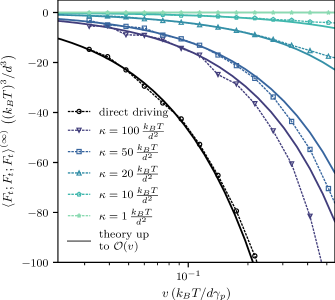
Figure 6: Third force cumulant as a function of driving velocity for the scenario of direct (black) and indirect driving (colors). Open symbols with dashed lines show results from non-equilibrium simulations. Lines correspond to response curves up to linear order obtained from equilibrium simulations (according to Eq. (20)). In the limit $v\to 0$ all curves converge to zero due to the symmetries of the equilibrium case.

Higher-order force cumulants quantify non-Gaussian fluctuations. As an example we consider the steady-state third force cumulant $\langle F_{t};F_{t};F_{t}\rangle^{(\infty)}$ evaluated at equal times, found from Eq. (20). Due to the equal times the expression for the respective first-order memory kernels simplifies to

$$\Gamma^{(2,1)}_{s;0,0}=\beta^{4}\left\langle F_{s};F_{0};F_{0};F_{0}\right\rangle_{\mathrm{eq}}.$$ (40)

Fig. 6 shows $\langle F_{t};F_{t};F_{t}\rangle^{(\infty)}$ as a function of driving velocity for direct driving (black) and indirect driving for different stiffness $\kappa$ (colors). We compare curves from non-equilibrium simulations (open symbols with dashed lines) with theoretical response curves up to linear order according to Eq. (20) (solid lines). In the limit $v\to 0$ the third force cumulant vanishes for both scenarios due to symmetry; the force distributions are symmetric in equilibrium. For finite driving Fig. 6 shows non-Gaussian behavior, whose amplitude increases with $\kappa$ and is particularly strong in the scenario of direct driving. We attribute this to the fact that in the scenario of direct driving the interaction potential is nonlinear.

V.6 Non-commutation of limits $\kappa\to\infty$ and $t\to 0$

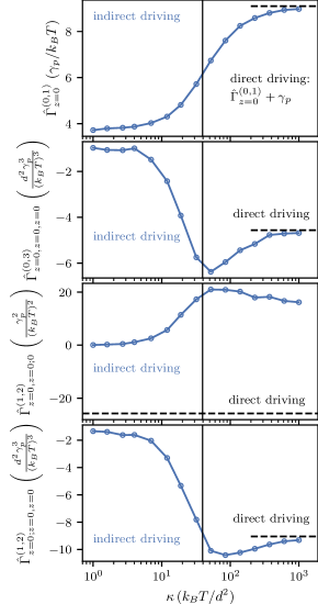
Figure 7: Integrated memory kernels $\hat{\Gamma}_{z=0}^{(0,1)}$ (top), $\hat{\Gamma}^{(0,3)}_{z=0,z=0,z=0}$ (second), $\hat{\Gamma}^{(1,2)}_{z=0,z=0;0}$ (third) and $\hat{\Gamma}^{(1,2)}_{z=0;z=0,z=0}$ (bottom) of mean force $\beta\langle F_{t}\rangle^{(\infty)}$, force variance $\beta^{2}\langle F_{t};F_{t}\rangle^{(\infty)}$ and integrated force covariance $\beta^{2}\langle\hat{F}_{z=0};F_{0}\rangle^{(\infty)}$ as a function of $\kappa$ for the scenario of indirect driving. The black dashed lines show resulting values for the scenario of direct driving. In the first panel $\gamma_{p}$ has been added to $\hat{\Gamma}^{(0,1)}_{z=0}$ for direct driving. The vertical line corresponds to $\kappa=\frac{2\pi^{2}U_{0}}{d^{2}}\approx 39k_{B}T/d^{2}$, half the curvature of the interaction potential $U_{\mathrm{int}}$ in the minimum.

We have in Secs. V.3-V.5 observed that in some cases, the limit of $\kappa\to\infty$ agrees with the case of direct driving, and in some cases, it does not. In this subsection, we analyze this in more detail, along with Fig. 7.

In the limit of $\kappa\to\infty$, the probe particle follows a prescribed velocity, so that the scenarios are expected to be identical. Furthermore, the force balance between bath particle and probe particle implies that the first cumulant, i.e., the mean force, agrees in that limit in the two cases. Indeed, the flow curve $\gamma(v)$ for indirect driving approaches the one of direct driving in the limit of $\kappa\to\infty$, see the two upper panels in Fig. 7; $\hat{\Gamma}_{z=0}^{(0,1)}$ and $\hat{\Gamma}^{(0,3)}_{z=0,z=0,z=0}$ are the leading contributions to the flow curve for small $v$ (compare Eq. (35), with $\gamma_{p}$ added in the direct case), and the graphs show that the cases of indirect driving reaches the direct case for large $\kappa$.

The situation is different for the force variance. Here, even in equilibrium, $\langle F_{t};F_{t}\rangle_{\rm eq}$ in Eq. (37) does not approach the case of direct driving of Eq. (39) for large $\kappa$ (as observed in Fig. 4). We recall that this difference in the force variance is an interesting feature showing that the direct case may allow experimental investigation of the interaction potential between particle and its surrounding. Also for finite velocity, $\langle F_{t};F_{t}\rangle^{(\infty)}$ for the indirect case does not approach the direct case for large $\kappa$, as demonstrated in Fig. 4 and in the third panel of Fig. 7; $\hat{\Gamma}^{(1,2)}_{z=0,z=0;0}$ describes the leading non-equilibrium contribution to that quantity, and, as seen, the two cases do not agree for large $\kappa$.

Does this observation of the limit of $\kappa\to\infty$ not reaching the case of direct driving violate the mentioned force balance? This might be understood by using the equilibrium case, Eqs. (37) and (39). These two equations result of equilibrium Boltzmann distributions of two distinct potentials, the harmonic trapping potential on one side, and the nonlinear interaction potential on the other. These thus lead to distinctly different results for the variance. The force balance comes however into play for finite time $t$ in $\langle F_{t};F_{0}\rangle^{(\infty)}$. If $\kappa$ is large, we observe the force covariance for the indirect case to follow $\langle F_{t};F_{0}\rangle^{(\infty)}\propto e^{-\frac{\kappa}{\gamma_{p}}t}$ for $t\ll\gamma_{p}/\kappa$, and to agree with the result of the direct case for $t\gtrsim\gamma_{p}/\kappa$. In other words the time period, where the two functions disagree, gets shorter and shorter, as $\kappa$ increases. We can thus state that limits of $\kappa\to\infty$ and $t\to 0$ seem not to commute. Setting $t=0$ in $\langle F_{t};F_{0}\rangle^{(\infty)}$ yields no agreement of the two cases for any $\kappa$, while, for any finite $t$, the two cases approach each other in the limit of $\kappa\to\infty$.

This can be illustrated by regarding the time integral, $\int_{0}^{\infty}\mathrm{d}t\,\langle F_{t};F_{0}\rangle^{(\infty)}$. For $v=0$, i.e., in equilibrium, this equals the $v\to 0$ limit of the flow curve, via FDT; thus, indeed, the cases approach each other in the limit of $\kappa\to\infty$ (taking into account the addition of $\gamma_{p}$ in the direct case). The leading non-equilibrium contribution to $\int_{0}^{\infty}\mathrm{d}t\,\langle F_{t};F_{0}\rangle^{(\infty)}$ is given by the integrated kernel $\hat{\Gamma}^{(1,2)}_{z=0;z=0,z=0}$, shown in the lowest panel of Fig. 7. We see that the two cases indeed approach each other for $\kappa\to\infty$.

The non-commutativity of the limits $\kappa\to\infty$ and $t\to 0$ can be further illustrated by comparing Figs. 5(b) and 9 in Appendix D, i.e. the transient force covariance in the two scenarios, using a quite large value of $\kappa=100\,k_{B}T/d^{2}$. The two graphs are similar despite an additional fast initial decay in the scenario of indirect driving, following the mentioned behavior $\langle F_{t};F_{0}\rangle\approx\kappa k_{B}Te^{-\frac{\kappa}{\gamma_{p}}t}$. For longer times the curves for the two scenarios fall on top of each other.

We conclude with another interesting aspect of Fig. 7. The graphs include vertical lines marking the point where $\kappa$ equals half the curvature of the interaction potential, i.e., $\kappa=\frac{1}{2}U_{\rm int}^{\prime\prime}(0)=\frac{2\pi^{2}U_{0}}{d^{2}}$. Interestingly, the curves show pronounced changes around this value. We may thus expect that, in experiments, the kernels strongly depend on $\kappa$ when $\kappa$ is comparable to the curvature of the interaction potential with the surrounding.

VI Conclusion

We derive nonlinear Langevin functionals for the cumulants of the stochastic force acting on a driven controlled degree of freedom, in a surrounding of Brownian particles. These nonlinear Langevin funtionals, Eqs. (18)-(20), are of the form of Volterra series in the velocity of the control parameter. We provide them explicitly up to third order in driving velocity, and highlight that respective kernels are given in terms of connected correlation functions; These follow from general nonlinear response formulas in terms of connected correlation functions derived here, and which we find to cancel divergences in the examples investigated.

We highlighted and discussed the specific scenarios of direct and indirect driving of a Brownian probe, using simulations of the stochastic Prandtl-Tomlinson model to explicitly evaluate and verify the kernels of Eqs. (18)-(20) in several limiting cases for the two scenarios. We find that qualitative nonlinear phenomena, such as shear-thinning and oscillations in the force covariance already appear in the memory kernels of third or second order.

We find that the force variance reveals interesting differences between the two cases of direct and indirect driving, and in particular, the direct case allows to infer information about the interaction potential of probe and surrounding. When regarded as a function of time difference $t$, this variance appears to be continuous in $\kappa$ for finite time $t$, meaning that the indirect case approaches the direct one for $\kappa\to\infty$, while the two cases remain different at $t=0$. We interpret that the limits of $\kappa\to\infty$ and $t\to 0$ do not commute, an effect which becomes apparent in the force fluctuations, but not in the mean force.

With Eqs. (18)-(21) we have established a complete theoretical framework for studying nonlinear and non-equilibrium fluctuations in overdamped Brownian baths, which opens up rich possibilities for further investigations, for example different driving protocols or coupling of different driven degrees of freedom, i.e., multidimensional controlled degrees. It will also be important to find whether the series expansion in terms of connected correlation functions can be extended to higher orders. One may also investigate whether time derivatives appearing in the correlation functions can be replaced [65].

Author declarations

Conflict of interest

The authors have no conflicts to disclose.

Author Contributions

Juliana Caspers: Formal Analysis, Investigation, Software, Visualization, Writing - Original Draft.
Matthias Krüger: Conceptualization, Methodology, Writing – Review & Editing.

Data availability

The data that support the findings of this study are available from the corresponding author upon reasonable request.

Appendix A Connected correlation functions

The response relations Eqs. (14) and (15) must hold for any state observable $O_{t}$, e.g. also for $O=1$. We can thus retrieve a list of identities that entropic and NT components must obey,

$$\langle S^{\prime}\rangle_{\mathrm{eq}}=\langle D^{\prime}\rangle_{\mathrm{eq}} =0$$ (41)

$$\langle D^{\prime}S^{\prime}\rangle_{\mathrm{eq}} =0$$ (42)

$$\left\langle D^{\prime\prime}-D^{\prime 2}-\frac{S^{\prime}}{4}\right\rangle_{\mathrm{eq}} =0$$ (43)

$$\left\langle D^{\prime 2}S^{\prime}-D^{\prime\prime}S^{\prime}+\frac{S^{\prime 2}}{12}\right\rangle_{\mathrm{eq}} =0.$$ (44)

$$\;\;\vdots$$

Let us calculate the covariance $\langle A;B\rangle\coloneqq\langle AB\rangle-\langle A\rangle\langle B\rangle$ for the first-order term in the response relation for a state observable, Eq. (15). We find $\langle S^{\prime};O_{t}\rangle_{\mathrm{eq}}=\langle S^{\prime}O_{t}\rangle_{\mathrm{eq}}$ using Eq. (41). For the second-order response we consider the joint cumulant or connected correlation function of third order, which is defined according to

$$\begin{split}\langle A;B;C\rangle&\coloneqq\langle ABC\rangle-\langle AB\rangle\langle C\rangle-\langle AC\rangle\langle B\rangle\\ &\quad-\langle A\rangle\langle BC\rangle+2\langle A\rangle\langle B\rangle\langle C\rangle.\end{split}$$ (45)

We find $\langle D^{\prime};S^{\prime};O_{t}\rangle_{\mathrm{eq}}=\langle D^{\prime}S^{\prime}O_{t}\rangle_{\mathrm{eq}}$ using Eqs. (41),(42). For the first two orders the expressions in terms of connected correlation functions follow trivially, because additional terms vanish individually. This is different for the third-order terms. We find

$$\begin{split}\frac{1}{6}\left\langle\left[3D^{\prime 2}-3D^{\prime\prime}+\frac{S^{\prime 2}}{4}\right]S^{\prime}O_{t}\right\rangle_{\mathrm{eq}}\quad\quad\quad\quad&\\ =\frac{1}{2}\Big{[}\langle D^{\prime};D^{\prime};S^{\prime};O_{t}\rangle_{\mathrm{eq}}-\langle D^{\prime\prime};S^{\prime};O_{t}\rangle_{\mathrm{eq}}&\\ +\frac{1}{12}\langle S^{\prime};S^{\prime};S^{\prime};O_{t}\rangle_{\mathrm{eq}}&\Big{]},\end{split}$$ (46)

but the three terms cannot be replaced with connected correlation functions individually, i.e. $\langle D^{\prime};D^{\prime};S^{\prime};O_{t}\rangle\neq\langle D^{\prime 2}S^{\prime}O_{t}\rangle_{\mathrm{eq}}$, $\langle D^{\prime\prime};S^{\prime};O_{t}\rangle_{\mathrm{eq}}\neq\langle D^{\prime\prime}S^{\prime}O_{t}\rangle_{\mathrm{eq}}$ and $\langle S^{\prime};S^{\prime};S^{\prime};O_{t}\rangle_{\mathrm{eq}}\neq\langle S^{\prime 3}O_{t}\rangle_{\mathrm{eq}}$. Eq. (46) contains the connected correlation function of fourth order. We do not give its definition explicitly, but provide the general definition of the connected correlation function of order $n$ [66],

$$\langle A_{1};\dots;A_{n}\rangle\coloneqq\sum_{\pi}(|\pi|-1)!(-1)^{|\pi|-1}\prod_{B\in\pi}\left\langle\prod_{i\in B}A_{i}\right\rangle$$ (47)

with the sum over all partitions $\{1,\dots,n\}$. $|\pi|$ denotes the number of parts in a partition and $B$ refers to all blocks of a partition.

Inserting all relations, we can express Eq. (15) in terms of connected correlation functions only and arrive at Eq. (16). The derivation of a response relation for a general path observable up to second order, Eq. (17), follows in analogy.

Appendix B $n-$th order memory kernel

In this appendix we set $\dot{x}_{t}\coloneqq\varepsilon\dot{\tilde{x}}_{t}$, with $\varepsilon$ defined as the dimensionless strength of perturbation. This allows to expand and take derivatives with respect to $\varepsilon$, which is simpler than considering time-dependent velocities. With this setting the non-equilibrium average of the force can be expressed as

$$\begin{split}\langle F_{t}\rangle=\underbrace{\langle F_{t}\rangle_{\mathrm{eq}}}_{=0}+\sum_{n=1}^{\infty}\frac{\varepsilon^{n}}{n!}\Bigg{\langle}\frac{\mathrm{d}^{n}}{\mathrm{d}\varepsilon^{n}}\Big{(}e^{-\varepsilon D^{\prime}(\omega)+\frac{\varepsilon}{2}S^{\prime}(\omega)-\frac{\varepsilon^{2}}{2}D^{\prime\prime}(\omega)}\quad&\\ -e^{-\varepsilon D^{\prime}(\omega)-\frac{\varepsilon}{2}S^{\prime}(\omega)-\frac{\varepsilon^{2}}{2}D^{\prime\prime}(\omega)}\Big{)}\Bigg{|}_{\varepsilon=0}F_{t}\Bigg{\rangle}_{\mathrm{eq}}&\end{split}$$ (48)

by expanding the perturbed action $\mathcal{A}_{\varepsilon}$ in a Taylor series in $\varepsilon$, $\mathcal{A}_{\varepsilon}=\varepsilon D^{\prime}-\varepsilon S^{\prime}/2+\varepsilon^{2}D^{\prime\prime}/2$ [63].

Applying general Leibniz rule on the $n-$th derivative of the exponential we can write [63]

$$\begin{split}\langle F_{t}\rangle&=\sum_{n=1}^{\infty}\frac{\varepsilon^{n}}{n!}\Bigg{\langle}\sum_{i=0}^{n}\binom{n}{i}\frac{\mathrm{d}^{n-i}}{\mathrm{d}\varepsilon^{n-i}}e^{-\varepsilon D^{\prime}(\omega)-\frac{\varepsilon^{2}}{2}D^{\prime\prime}(\omega)}\Bigg{|}_{\varepsilon=0}\\ &\quad\times\left[\left(\frac{S^{\prime}(\omega)}{2}\right)^{i}-\left(-\frac{S^{\prime}(\omega)}{2}\right)^{i}\right]F_{t}\Bigg{\rangle}_{\mathrm{eq}}.\end{split}$$ (49)

Let us first consider the NT part. From Faà di Bruno’s formula expressed in terms of complete Bell polynomials $B_{n}$, $\frac{\mathrm{d}^{n}}{\mathrm{d}x^{n}}e^{f(x)}=e^{f(x)}B_{n}(f^{\prime}(x),f^{\prime\prime}(x),\dots,f^{(n)}(x))$ [67] we find

$$\begin{split}\frac{\mathrm{d}^{n-i}}{\mathrm{d}\varepsilon^{n-i}}&e^{-\varepsilon D^{\prime}(\omega)-\frac{\varepsilon^{2}}{2}D^{\prime\prime}(\omega)}\Bigg{|}_{\varepsilon=0}\\ &\quad\quad\quad=B_{n-i}\left(-D^{\prime},-D^{\prime\prime},0,\dots,0\right).\end{split}$$ (50)

Eq. (50) thus contains $n-i$ integrals which can be taken out of the Bell polynomials when functional derivatives are applied,

$$\frac{\mathrm{d}^{n-i}}{\mathrm{d}\varepsilon^{n-i}}e^{-D(\omega)}\Bigg{|}_{\varepsilon=0}=\frac{1}{(n-i)!}\int_{t_{0}}^{t}\mathrm{d}s_{1}\cdots\int_{t_{0}}^{t}\mathrm{d}s_{n-i}\,\dot{x}_{s_{1}}\cdots\dot{x}_{s_{n-i}}\frac{\delta^{n-i}}{\delta\dot{x}_{s_{1}}\cdots\delta\dot{x}_{s_{n-i}}}B_{n-i}\left(-D^{\prime},-D^{\prime\prime},0,\dots,0\right).$$ (51)

The entropic part takes on the form

$$\left(\frac{S^{\prime}(\omega)}{2}\right)^{i}-\left(-\frac{S^{\prime}(\omega)}{2}\right)^{i}=\left(\frac{\beta}{2}\right)^{i}\left(1-(-1)^{i}\right)\int_{t_{0}}^{t}\mathrm{d}s_{1}\cdots\int_{t_{0}}^{t}\mathrm{d}s_{i}\,\dot{x}_{s_{1}}\cdots\dot{x}_{s_{i}}F_{s_{1}}\cdots F_{s_{i}}.$$ (52)

Inserting Eqs. (51) and (52) back into Eq. (49) we obtain

$$\begin{split}\langle F_{t}\rangle&=\sum_{n=1}^{\infty}\frac{\varepsilon^{n}}{n!}\int_{t_{0}}^{t}\mathrm{d}s_{1}\cdots\int_{t_{0}}^{t}\mathrm{d}s_{n}\,\dot{x}_{s_{1}}\cdots\dot{x}_{s_{n}}\sum_{i=1}^{n}\frac{\left(1-(-1)^{i}\right)}{(n-i)!}\binom{n}{i}\left(\frac{\beta}{2}\right)^{i}\\ &\quad\times\left\langle\frac{\delta^{n-i}}{\delta\dot{x}_{t-s_{1}}\cdots\delta\dot{x}_{t-s_{n-i}}}B_{n-i}\left(D^{\prime},-D^{\prime\prime},0,\dots,0\right)F_{t-s_{n-i+1}}\cdots F_{t-s_{n}}F_{0}\right\rangle_{\mathrm{eq}},\end{split}$$ (53)

where we have shifted all time arguments by time $t$ and applied time-reversal (resulting in a change of sign of NT components of even order) to follow the notation in Eqs. (18)-(20). Applying Eq. (21), the $n-$th order memory kernel for the mean force can thus be expressed as

$$\begin{split}\Gamma_{s_{1},\dots,s_{n}}^{(0,n)}=&\frac{\beta}{(n!)^{2}}\sum_{\pi\in S_{n}}\sum_{i=1}^{n}\frac{\left(1-(-1)^{i}\right)}{(n-i)!}\binom{n}{i}\left(\frac{\beta}{2}\right)^{i}\\ &\times\left\langle\frac{\delta^{n-i}}{\delta\dot{x}_{s_{\pi(1)}}\cdots\delta\dot{x}_{s_{\pi(n-i)}}}B_{n-i}\left(D^{\prime},-D^{\prime\prime},0,\dots,0\right)F_{s_{\pi(n-i+1)}}\cdots F_{s_{\pi(n)}}F_{0}\right\rangle_{\mathrm{eq}}.\end{split}$$ (54)

Note that the notion of connected correlation functions is not included in the above derivation. Eq. (54) expresses $\Gamma^{(0,n)}$ in terms of equilibrium correlation functions only.

Appendix C Convergence of connected correlation functions

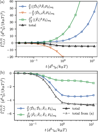
Figure 8: Running integral of the third-order memory kernel $\tilde{\Gamma}^{(0,3)}_{t,t,t}=\int_{0}^{t}\mathrm{d}s\int_{0}^{t}\mathrm{d}s^{\prime}\int_{0}^{t}\mathrm{d}s^{\prime\prime}\,\Gamma_{s,s^{\prime},s^{\prime\prime}}^{(0,3)}$ calculated using (a) the (standard) response relation, Eq. (15), and (b) the response relation in terms of connected correlation functions, Eq. (16). Colored curves show individual terms and black curves their total. The dotted lines are identical in (a) and (b) and indicate the limit $\lim_{t\to\infty}\tilde{\Gamma}_{t,t,t}^{(0,3)}$ used for further analysis. The black line from (a) is added as dashed gray line to (b).

How can we obtain the time-integrated kernel $\hat{\Gamma}^{(0,3)}_{z=0,z=0,z=0}$ given by Eq. (24) efficiently? We first calculate running integrals $\tilde{A}_{t}\coloneqq\int_{0}^{t}\mathrm{d}s\,A_{s}$ and afterwards compute respective (connected) correlation functions as function of time $t$. We then check convergence and read off the long-time limit. First, we follow this approach to naively compute the running integral of $\Gamma^{(0,3)}$ over all times, $\tilde{\Gamma}^{(0,3)}_{t,t,t}=\int_{0}^{t}\mathrm{d}s\int_{0}^{t}\mathrm{d}s^{\prime}\int_{0}^{t}\mathrm{d}s^{\prime\prime}\,\Gamma_{s,s^{\prime},s^{\prime\prime}}^{(0,3)}$, via the response relation in terms of correlation functions, Eq. (15), i.e. Eq. (54) in Appendix B. The result for the scenario of direct driving is shown in Fig. 8(a). We observe convergence to $\hat{\Gamma}^{(0,3)}_{z=0,z=0,z=0}\approx-4.5\,d^{2}\gamma_{p}^{3}/(k_{B}T)^{3}$ for the total (black line), however the three individual terms diverge (colored lines). In contrast, when applying the response relation in terms of connected correlation functions, Eq. (16), we observe convergence of the individual terms as well, see Fig. 8(b). The curves for Fig. 8(a) and (b) were obtained in the same simulation, i.e. with identical statistics. The two total curves (black and gray lines) are almost identical and converge to the same limiting value. Connected correlation functions therefore have an important interpretation, but little influence on the convergence of the total response.

Appendix D Transient force covariance for the scenario of indirect driving

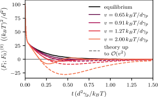
Figure 9: Transient force covariance for different driving velocities $v$ (colored lines) for the scenario of indirect driving with $\kappa=100\,k_{B}T/d^{2}$. Dashed lines show response curves according to Eq. (19) up to $\mathcal{O}(v^{2})$.

Fig. 9 shows simulations of the transient force covariance for different driving velocities $v$ (solid lines) for the scenario of indirect driving with $\kappa=100\,k_{B}T/d^{2}$. The dashed lines correspond to theoretical response curves up to second order according to Eq. (19). At time zero, we find $\langle F_{0};F_{0}\rangle^{(0)}=\kappa k_{B}T$ (compare Eq. (39)) which is followed by a fast decay $\propto e^{-\frac{\kappa}{\gamma_{p}}t}$ with the relaxation time of the bare probe in the trap. For larger driving velocity the force covariance exhibits clear oscillations in agreement with experiments in micellar systems [23, 24]. This phenomenon already appears in the second-order response (dashed lines).

References

References

- Dhont [1996] J. Dhont, An Introduction to Dynamics of Colloids (Elsevier Science, 1996).
- Baiesi, Iubini, and Orlandini [2021] M. Baiesi, S. Iubini, and E. Orlandini, “The rise and fall of branching: A slowing down mechanism in relaxing wormlike micellar networks,” The Journal of Chemical Physics 155, 214905 (2021).
- Ginot et al. [2022] F. Ginot, J. Caspers, L. F. Reinalter, K. K. Kumar, M. Krüger, and C. Bechinger, “Recoil experiments determine the eigenmodes of viscoelastic fluids,” New J. Phys. 24, 123013 (2022).
- Zwanzig [1961] R. Zwanzig, “Memory Effects in Irreversible Thermodynamics,” Phys. Rev. 124, 983–992 (1961).
- Mori [1965] H. Mori, “Transport, Collective Motion, and Brownian Motion,” Progress of Theoretical Physics 33, 423–455 (1965).
- Zwanzig [2001] R. Zwanzig, Nonequilibrium Statistical Mechanics (Oxford University Press, 2001).
- Grabert [1982] H. Grabert, Projection Operator Techniques in Nonequilibrium Statistical Mechanics, Springer Tracts in Modern Physics, Vol. 95 (Springer, Berlin, Heidelberg, 1982).
- Caldeira and Leggett [1981] A. O. Caldeira and A. J. Leggett, “Influence of Dissipation on Quantum Tunneling in Macroscopic Systems,” Phys. Rev. Lett. 46, 211–214 (1981).
- Götze [2008] W. Götze, Complex Dynamics of Glass-Forming Liquids: A Mode-Coupling Theory (Oxford University Press, 2008).
- Janssen [2018] L. M. C. Janssen, “Mode-Coupling Theory of the Glass Transition: A Primer,” Frontiers in Physics 6 (2018).
- Fuchs, Götze, and Mayr [1998] M. Fuchs, W. Götze, and M. R. Mayr, “Asymptotic laws for tagged-particle motion in glassy systems,” Phys. Rev. E 58, 3384–3399 (1998).
- van Zanten and Rufener [2000] J. H. van Zanten and K. P. Rufener, “Brownian motion in a single relaxation time Maxwell fluid,” Phys. Rev. E 62, 5389–5396 (2000).
- Lu and Solomon [2002] Q. Lu and M. J. Solomon, “Probe size effects on the microrheology of associating polymer solutions,” Phys. Rev. E 66, 061504 (2002).
- Van Der Gucht et al. [2003] J. Van Der Gucht, N. A. M. Besseling, W. Knoben, L. Bouteiller, and M. A. Cohen Stuart, “Brownian particles in supramolecular polymer solutions,” Phys. Rev. E 67, 051106 (2003).
- Caspers et al. [2023] J. Caspers, N. Ditz, K. Krishna Kumar, F. Ginot, C. Bechinger, M. Fuchs, and M. Krüger, “How are mobility and friction related in viscoelastic fluids?” J. Chem. Phys. 158, 024901 (2023).
- Doerries, Loos, and Klapp [2021] T. J. Doerries, S. A. M. Loos, and S. H. L. Klapp, Correlation functions of non-Markovian systems out of equilibrium: analytical expressions beyond single-exponential memory, J. Stat. Mech. 2021, 033202 (2021).
- Venturelli and Gambassi [2023] D. Venturelli and A. Gambassi, “Memory-induced oscillations of a driven particle in a dissipative correlated medium,” New J. Phys. 25, 093025 (2023).
- Squires and Brady [2005] T. M. Squires and J. F. Brady, “A simple paradigm for active and nonlinear microrheology,” Physics of Fluids 17, 073101 (2005).
- Gazuz et al. [2009] I. Gazuz, A. M. Puertas, T. Voigtmann, and M. Fuchs, “Active and Nonlinear Microrheology in Dense Colloidal Suspensions,” Phys. Rev. Lett. 102, 248302 (2009).
- Harrer et al. [2012] C. J. Harrer, D. Winter, J. Horbach, M. Fuchs, and T. Voigtmann, “Force-induced diffusion in microrheology,” J. Phys.: Condens. Matter 24, 464105 (2012).
- Jayaraman and Belmonte [2003] A. Jayaraman and A. Belmonte, “Oscillations of a solid sphere falling through a wormlike micellar fluid,” Phys. Rev. E 67, 065301 (2003).
- Handzy and Belmonte [2004] N. Z. Handzy and A. Belmonte, “Oscillatory Rise of Bubbles in Wormlike Micellar Fluids with Different Microstructures,” Phys. Rev. Lett. 92, 124501 (2004).
- Berner et al. [2018] J. Berner, B. Müller, J. R. Gomez-Solano, M. Krüger, and C. Bechinger, “Oscillating modes of driven colloids in overdamped systems,” Nat Commun 9, 999 (2018).
- Jain et al. [2021] R. Jain, F. Ginot, J. Berner, C. Bechinger, and M. Krüger, “Two step micro-rheological behavior in a viscoelastic fluid,” J. Chem. Phys. 154, 184904 (2021).
- Winter et al. [2012] D. Winter, J. Horbach, P. Virnau, and K. Binder, “Active Nonlinear Microrheology in a Glass-Forming Yukawa Fluid,” Phys. Rev. Lett. 108, 028303 (2012).
- Bénichou et al. [2013] O. Bénichou, A. Bodrova, D. Chakraborty, P. Illien, A. Law, C. Mejía-Monasterio, G. Oshanin, and R. Voituriez, “Geometry-Induced Superdiffusion in Driven Crowded Systems,” Phys. Rev. Lett. 111, 260601 (2013).
- Wilson and Poon [2011] L. G. Wilson and W. C. K. Poon, “Small-world rheology: an introduction to probe-based active microrheology,” Phys. Chem. Chem. Phys. 13, 10617–10630 (2011).
- Démery and Fodor [2019] V. Démery and E. Fodor, “Driven probe under harmonic confinement in a colloidal bath,” J. Stat. Mech. 2019, 033202 (2019).
- Cugliandolo [2011] L. F. Cugliandolo, “The effective temperature,” J. Phys. A: Math. Theor. 44, 483001 (2011).
- Puglisi, Sarracino, and Vulpiani [2017] A. Puglisi, A. Sarracino, and A. Vulpiani, “Temperature in and out of equilibrium: A review of concepts, tools and attempts,” Physics Reports 709-710, 1–60 (2017).
- Brader, Cates, and Fuchs [2008] J. M. Brader, M. E. Cates, and M. Fuchs, “First-Principles Constitutive Equation for Suspension Rheology,” Phys. Rev. Lett. 101, 138301 (2008).
- Krüger, Weysser, and Fuchs [2011] M. Krüger, F. Weysser, and M. Fuchs, “Tagged-particle motion in glassy systems under shear: Comparison of mode coupling theory and Brownian dynamics simulations,” Eur. Phys. J. E 34, 88 (2011).
- Gazuz and Fuchs [2013] I. Gazuz and M. Fuchs, “Nonlinear microrheology of dense colloidal suspensions: A mode-coupling theory,” Phys. Rev. E 87, 032304 (2013).
- Gruber et al. [2016] M. Gruber, G. C. Abade, A. M. Puertas, and M. Fuchs, “Active microrheology in a colloidal glass,” Phys. Rev. E 94, 042602 (2016).
- Meyer, Voigtmann, and Schilling [2017] H. Meyer, T. Voigtmann, and T. Schilling, “On the non-stationary generalized Langevin equation,” The Journal of Chemical Physics 147, 214110 (2017).
- te Vrugt and Wittkowski [2019] M. te Vrugt and R. Wittkowski, “Mori-Zwanzig projection operator formalism for far-from-equilibrium systems with time-dependent Hamiltonians,” Phys. Rev. E 99, 062118 (2019).
- Meyer, Voigtmann, and Schilling [2019] H. Meyer, T. Voigtmann, and T. Schilling, “On the dynamics of reaction coordinates in classical, time-dependent, many-body processes,” The Journal of Chemical Physics 150, 174118 (2019).
- Glatzel and Schilling [2021] F. Glatzel and T. Schilling, “The interplay between memory and potentials of mean force: A discussion on the structure of equations of motion for coarse-grained observables,” EPL 136, 36001 (2021).
- Vroylandt and Monmarché [2022] H. Vroylandt and P. Monmarché, “Position-dependent memory kernel in generalized Langevin equations: theory and numerical estimation,” J. Chem. Phys. 156, 244105 (2022).
- Schilling [2022] T. Schilling, “Coarse-grained modelling out of equilibrium,” Physics Reports Coarse-Grained Modelling Out of Equilibrium, 972, 1–45 (2022).
- Netz [2023] R. R. Netz, “Derivation of the non-equilibrium generalized Langevin equation from a generic time-dependent Hamiltonian,” (2023), arXiv:2310.00748 [cond-mat].
- Penna, Dzubiella, and Tarazona [2003] F. Penna, J. Dzubiella, and P. Tarazona, “Dynamic density functional study of a driven colloidal particle in polymer solutions,” Phys. Rev. E 68, 061407 (2003).
- Rauscher et al. [2007] M. Rauscher, A. Domínguez, M. Krüger, and F. Penna, “A dynamic density functional theory for particles in a flowing solvent,” The Journal of Chemical Physics 127, 244906 (2007).
- Gutsche et al. [2008] C. Gutsche, F. Kremer, M. Krüger, M. Rauscher, R. Weeber, and J. Harting, “Colloids dragged through a polymer solution: Experiment, theory, and simulation,” The Journal of Chemical Physics 129, 084902 (2008).
- De Las Heras and Schmidt [2018] D. De Las Heras and M. Schmidt, “Velocity Gradient Power Functional for Brownian Dynamics,” Phys. Rev. Lett. 120, 028001 (2018).
- De Las Heras and Schmidt [2020] D. De Las Heras and M. Schmidt, “Flow and Structure in Nonequilibrium Brownian Many-Body Systems,” Phys. Rev. Lett. 125, 018001 (2020).
- Schmidt [2022] M. Schmidt, “Power functional theory for many-body dynamics,” Rev. Mod. Phys. 94, 015007 (2022).
- Asheichyk, Fuchs, and Krüger [2021] K. Asheichyk, M. Fuchs, and M. Krüger, “Brownian systems perturbed by mild shear: comparing response relations,” J. Phys.: Condens. Matter 33, 405101 (2021).
- Krüger and Maes [2016] M. Krüger and C. Maes, “The modified Langevin description for probes in a nonlinear medium,” J. Phys.: Condens. Matter 29, 064004 (2016).
- Müller [2020] B. Müller, Brownian Particles in Nonequilibrium Solvents, Ph.D. thesis, Georg-August-Universität Göttingen (2020).
- Colangeli, Maes, and Wynants [2011] M. Colangeli, C. Maes, and B. Wynants, “A meaningful expansion around detailed balance,” J. Phys. A: Math. Theor. 44, 095001 (2011).
- Basu et al. [2015] U. Basu, M. Krüger, A. Lazarescu, and C. Maes, “Frenetic aspects of second order response,” Phys. Chem. Chem. Phys. 17, 6653–6666 (2015).
- Maes [2020a] C. Maes, “Response Theory: A Trajectory-Based Approach,” Frontiers in Physics 8 (2020a).
- Müller et al. [2020] B. Müller, J. Berner, C. Bechinger, and M. Krüger, “Properties of a nonlinear bath: experiments, theory, and a stochastic Prandtl–Tomlinson model,” New J. Phys. 22, 023014 (2020).
- Jain, Ginot, and Krüger [2021] R. Jain, F. Ginot, and M. Krüger, “Micro-rheology of a particle in a nonlinear bath: Stochastic Prandtl-Tomlinson model,” Physics of Fluids 33, 103101 (2021).
- Note [1] The minus sign is included because it will yield the familiar sign convention for the case of indirect driving introduced below.
- [57] Clemens Bechinger, personal communication, 2024.
- Maes [2020b] C. Maes, “Frenesy: Time-symmetric dynamical activity in nonequilibria,” Physics Reports Frenesy: time-symmetric dynamical activity in nonequilibria, 850, 1–33 (2020b).
- Onsager and Machlup [1953] L. Onsager and S. Machlup, “Fluctuations and Irreversible Processes,” Phys. Rev. 91, 1505–1512 (1953).
- Baiesi, Maes, and Wynants [2009] M. Baiesi, C. Maes, and B. Wynants, “Fluctuations and Response of Nonequilibrium States,” Phys. Rev. Lett. 103, 010602 (2009).
- Maes and Netočný [2003] C. Maes and K. Netočný, “Time-Reversal and Entropy,” Journal of Statistical Physics 110, 269–310 (2003).
- Seifert [2012] U. Seifert, “Stochastic thermodynamics, fluctuation theorems and molecular machines,” Rep. Prog. Phys. 75, 126001 (2012).
- Holsten and Krüger [2021] T. Holsten and M. Krüger, “Thermodynamic nonlinear response relation,” Phys. Rev. E 103, 032116 (2021).
- Kardar [2007] M. Kardar, Statistical Physics of Fields (Cambridge University Press, Cambridge, 2007).
- Asheichyk et al. [2019] K. Asheichyk, A. P. Solon, C. M. Rohwer, and M. Krüger, “Response of active Brownian particles to shear flow,” J. Chem. Phys. 150, 144111 (2019).
- Peccati and Taqqu [2011] G. Peccati and M. S. Taqqu, Wiener Chaos: Moments, Cumulants and Diagrams, Bocconi & Springer Series, Vol. 1 (Springer Milan, Milano, 2011).
- di Bruno [1855] F. di Bruno, “Sullo sviluppo delle funzioni,” Ann. Sci. Mat. Fis., Roma 6, 479–480 (1855).