Unraveling the role of merger histories in the population of Insitu stars: linking IllustrisTNG cosmological simulation to H3 survey

Abstract

We undertake a comprehensive investigation into the distribution of insitu stars within Milky Way-like galaxies, leveraging TNG50 simulations and comparing their predictions with data from the H3 survey. Our analysis reveals that 28% of galaxies demonstrate reasonable agreement with H3, while only 12% exhibit excellent alignment in their profiles, regardless of the specific spatial cut employed to define insitu stars. To uncover the underlying factors contributing to deviations between TNG50 and H3 distributions, we scrutinize correlation coefficients among internal drivers(e.g., virial radius, star formation rate [SFR]) and merger-related parameters (such as the effective mass-ratio, mean distance, average redshift, total number of mergers, average spin-ratio and maximum spin alignment between merging galaxies). Notably, we identify significant correlations between deviations from observational data and key parameters such as the median slope of virial radius, mean SFR values, and the rate of SFR change across different redshift scans. Furthermore, positive correlations emerge between deviations from observational data and parameters related to galaxy mergers. We validate these correlations using the Random Forest Regression method. Our findings underscore the invaluable insights provided by the H3 survey in unraveling the cosmic history of galaxies akin to the Milky Way, thereby advancing our understanding of galactic evolution and shedding light on the formation and evolution of Milky Way-like galaxies in cosmological simulations.

revtex4-1.clsrevtex4-2.cls

1 Introduction

The stellar distribution within the Milky Way (MW) galaxy offers valuable insights into its merger history. By combining photometric observations with stellar kinematics, we can reconstruct the accretion history of the MW. Within the MW, stellar components may originate from its main galaxy, including those formed from accreted gas, known as insitu stars, or they may be accreted from satellite galaxies, termed ex-situ stars. Understanding whether the MW is predominantly composed of insitu stars or enriched by ex-situ components provides a crucial avenue for advancing theories of galaxy formation and evolution.

The origin of the Milky Way’s stellar halo has been a focus of theoretical investigation in several studies. Utilizing Sloan Digital Sky Survey (SDSS) Data Release 5 (DR5), Bell et al. (2008) observed that the structure of the MW’s stellar halo resembles debris from a disrupted satellite galaxy, suggesting a substantial contribution from tidally disrupted galaxies. This conclusion was supported by Mackereth et al. (2019), who employed abundance data from APOGEE-DR14 and kinematic data from Gaia-DR. Additionally, Kisku et al. (2021) analyzed APOGEE data, focusing on the chemical composition of N-rich stars, and estimated that approximately 30% of the inner galactic stars originated from disrupted globular clusters (GCs). Furthermore, Matsuno et al. (2019) identified a population of retrograde, metal-poor stars potentially originating from accreted dwarf galaxies, contributing to the understanding of the MW’s stellar halo formation.

Numerous studies have investigated the fraction of insitu stars in the Milky Way galaxy (see, for example, Zolotov et al., 2009; Purcell et al., 2010; Cooper et al., 2015; Pillepich et al., 2015; Monachesi et al., 2019; Fattahi et al., 2020, and references therein). These analyses have yielded a wide range of inferred values for the insitu component, with simulations suggesting it can vary greatly, from being relatively negligible to nearly comparable to the accreted stellar components.

Observationally, recent advancements in stellar spectroscopic surveys, including RAVE (Steinmetz et al., 2006), SEGUE (Yanny et al., 2009), LAMOST (Cui et al., 2012), GALAH (De Silva et al., 2015), APOGEE (Majewski et al., 2017), Gaia (Gaia Collaboration et al., 2016), and H3 (Conroy et al., 2019b, a), have provided precise information regarding the position, velocity, and chemical abundances of millions of stars in the solar neighborhood.

Building upon insights from the H3 survey, Naidu et al. (2020) demonstrated that the MW is predominantly composed of substructures that have been accreted onto the galaxy. They specifically analyzed the chemical abundance of stars spanning from the local halo to the extended stellar halo, shedding light on their origins.

Expanding on these findings regarding the origins of individual stars, the question arises concerning the origin and nature of the stellar halo. Specifically, there is a debate over whether the halo consists mainly of insitu or ex-situ stars (see, for example, Eggen et al., 1962; Searle & Zinn, 1978; Ishigaki et al., 2021; Carollo & Chiba, 2021; Matteucci, 2021, and references therein). Additionally, understanding the radial extent of insitu and ex-situ stars, along with their relative ratios in the MW galaxy, provides insights into the MW’s accretion history. Recent studies, such as Han et al. (2022), have shown that the accreted stellar halo in the MW is tilted, adding further complexity to our understanding of its formation and evolution.

In this study, we conduct an in-depth analysis of insitu stars in 25 Milky Way-like galaxies simulated using the TNG50 run of the IllustrisTNG simulation (Pillepich et al., 2019; Nelson et al., 2019a). We quantify the distribution of the insitu star fraction and compare it with recent observational data from the Hectochelle in Halo at the High Resolution survey, hereafter the H3 survey, Naidu et al. (2020). By employing various spatial cuts, we find that 28% of galaxies in our sample exhibit reasonable agreement with the observational data, while only 12% show excellent alignment between theory and observation. We investigate the underlying factors contributing to the deviation between TNG50 results and the H3 survey outcomes for the scale height dependencies of the insitu star fraction. This analysis involves correlating the deviation with internal drivers such as the virial radius and star formation rate, along with external parameters related to mergers, including merger mass-ratio, mean merging galaxy distance, effective merger redshift, total number of mergers, mean spin fraction, and maximum alignment of merging galaxy spins. Our findings reveal significant correlations between these parameters and the deviation from H3 observations, underscoring the utility of H3 results in providing valuable constraints on galaxy evolution.

The paper is organized as follows. Section 2 presents an overview of the TNG simulation as well as the H3 survey. Section 3, introduces the insitu stars from the TNG50 simulation, and Section 4, explores the origin of the discrepancies between the simulation and observations. Section 5 presents the conclusion of the paper. Several technical details are presented in Appendices A and B.

2 Sample selection in TNG vs the selection functions in H3

In this section, we provide a summary of the sample selections made from both the TNG50 simulation and the H3 survey. These selections form the foundation of the analysis presented throughout the remainder of the paper.

2.1 Milky Way-like galaxies in TNG50

The IllustrisTNG simulations represent the next generation of cosmological hydrodynamical simulations designed to model galaxy formation and evolution within the framework of the $\Lambda$CDM paradigm (Pillepich et al., 2019; Nelson et al., 2019a). Building upon the foundations laid by the earlier Illustris simulations (Vogelsberger et al., 2014a, b; Genel et al., 2014; Sijacki et al., 2015), IllustrisTNG incorporates significant improvements, particularly in the modeling of AGN feedback, chemical enrichment, and the evolution of seed magnetic fields (Weinberger et al., 2017; Pillepich et al., 2018).

In this paper, we concentrate on the TNG50 simulation that operates within a periodic box with a size of L_box = 35 Mpc/h, containing 2160³ gas and dark matter particles with mass resolutions of [0.85, 4.5] $\times 10^{5}M_{\odot}$, respectively. Moreover, TNG50 adopts the cosmological parameters specified by Planck Collaboration et al. (2016). This simulation provides a detailed and comprehensive framework for studying the formation and evolution of galaxies across cosmic time.

We examine a carefully selected sample of 25 Milky Way-like galaxies from TNG50 identified and characterized in previous works (Emami et al., 2020a, b, 2022; Waters et al., 2024). Our sample selection adheres to two primary criteria. Firstly, we constrain the dark matter halo mass to fall within the range of (1-1.6)$\times 10^{12}M_{\odot}$, motivated by recent observational constraints on the dark matter halo mass of the Milky Way galaxy (Posti & Helmi, 2019). Secondly, we limit our galaxy sample to rotationally supported galaxies exhibiting a predominant stellar disk structure, identified using the orbital circularity parameter (see, e.g. Abadi et al., 2003; El-Badry et al., 2018). These selection criteria have been extensively discussed in prior studies (Emami et al., 2020a, b), with detailed formulations provided in Eqs. (1-2) of Emami et al. (2020b).

2.2 H3 observation and selection functions

The H3 (Hectochelle in Halo at the High Resolution) Survey is an ongoing stellar spectroscopic survey that offers an unbiased measurement of stellar parameters (Conroy et al., 2019b, a). It provides spectro-photometric distances for approximately 2$\times 10^{5}$ stars within the photometric magnitude range of $15<r<18$, with a 3D heliocentric distance of d${}_{\mathrm{helio}}>$ 3 kpc, $|b|>40^{\circ}$, and Dec $>-20^{\circ}$. H3 survey outputs radial velocities, spectroscopic distances, [Fe/H], and [$\alpha$/Fe] abundances for the aforementioned stellar sample. By combining this data with the Gaia proper motion measurements, enables the determination of the full 6D phase-space information and 2D chemical-space information for these stars.

In a related study, Naidu et al. (2020) focused on 5684 K giants from the H3 survey and conducted an extensive exploration of the structure of distant galaxies up to 50 kpc from the galactic center. They analyzed the scale-height dependence of the insitu stars. Naidu et al. (2020) used a dedicated approach, combining the kinematics information as well as the metallicity and made a general class of insitu stars including the contributions from different parts such as the high-$\alpha$ disk, insitu halo, the metal-weak thick disk, Aleph, and unclassified disk debris.

Motivated by these observational findings, our study investigates insitu stars within a selected sample of Milky Way-like galaxies from the TNG50 simulation. We focus on assessing the scale height dependence of the insitu star fraction and contrasting our results with those from the H3 survey. While the H3 survey employed a combination of the kinematics and chemical cuts involving [Fe/H] and [$\alpha$/Fe] abundances, alongside photometric magnitude, in this first study, our approach to identifying insitu stars within the TNG50 simulations is based on their birth location within the first progenitor throughout the cosmic evolution and within a given radial cut. Following the notation of De Lucia & Blaizot (2007), the first progenitor is the one with the “most massive history" behind it, while the second progenitor is defined as the galaxy with the second massive history behind it. In this paper, we often refer to the first ($f$) and second progenitor ($s$). Furthermore, to facilitate comparison with the H3 findings, we add similar spatial selection functions and study the role of varying radial cutoffs to compile a sample of insitu stars in our galaxy dataset. Subsequently, we conduct a comparative analysis of the scale height profile of insitu stars with the H3 survey results, representing their distance from the galactic disk plane.

3 Theoretical estimation of insitu stars

3.1 Inferring the insitu stars from TNG50 simulation

The insitu stellar component comprises stars born within the disk of their galactic host halo, as well as stars formed from streams of stripped gas originating from infalling satellites (Benson et al., 2004; Zolotov et al., 2009; Purcell et al., 2010; McCarthy et al., 2012; Tissera et al., 2014; Pillepich et al., 2015; Rodriguez-Gomez et al., 2016; Monachesi et al., 2019). Insitu stars born in the disk may be ejected to larger distances due to interactions with the molecular clouds. The amount of ejected mass strongly depends on subgrid physics and stellar feedback (see, for instance, Zolotov et al., 2009; Cooper et al., 2015, and references therein). Consequently, the radial profile of the fraction of insitu stars varies among different simulations, ranging from negligible at larger distances ($>5$ kpc) (Zolotov et al., 2009; Pillepich et al., 2015) to dominant at larger radii (Font et al., 2011; Monachesi et al., 2016b, a; Elias et al., 2018; Monachesi et al., 2019). On the contrary, accreted stars are born in satellite galaxies, with the satellite either bound to the main progenitor from the outset or accreted into the main progenitor at a later time (see, for example, Tissera et al., 2014; Monachesi et al., 2019, and references therein).

In the following, we present our strategy for selecting the insitu stars for a sample of 25 MW-like galaxies in the TNG50 simulation. The insitu star fraction is defined as the ratio of insitu stars to the total number of stars at that location. For more details about our sample selection, please refer to Sec. 2.1.

We utilize merger trees constructed from the sublink algorithm (Rodriguez-Gomez et al., 2015, 2016) to identify the main progenitors of the subhalo, which are defined as the most massive progenitor of the target subhalo at any given cosmic time (De Lucia & Blaizot, 2007). Furthermore, we employ baryonic merger trees, tracking only the stellar components in our analysis. As previously mentioned, we exclusively consider stars belonging to the main progenitor. Specifically, we initiate with the stellar components bound to the main halo at zero redshift, $z=0$, and trace their birth locations backward in time. Subsequently, we ascertain whether each star was part of the main progenitor at its birth time. Finally, we determine the distance of the star from its host galaxy at its birth time and compare it with a radial threshold, denoted as $r_{\mathrm{cut}}$. We employ four different selections for $r_{\mathrm{cut}}$, encompassing either a constant value of $30$ kpc or three time-dependent distances defined as some fixed coefficient of the virial distance (hereafter $R_{\mathrm{vir}}$) at the star’s birth time; further details are provided below. If the star is situated within the specified threshold, we categorize it as an insitu star; otherwise, it is considered as being accreted onto the main halo.

3.2 Redshift evolution of the main progenitor

As previously mentioned, we utilize the merger trees generated by the sublink algorithm to investigate the merger history for the first and second progenitors of all halos in our MW-like sample. Through this process, we determine the mass-ratio and merger time for each merger event. Following the standard methodology outlined in Rodriguez-Gomez et al. (2015, 2016), the mass-ratio in a merger system is determined when the second progenitor reaches its maximum mass. However, estimating the precise merger time is more intricate, as the second progenitor may orbit around the first progenitor and subsequently lose a significant portion of its mass. In our analysis below, we compute all correlation coefficients at the point when the second progenitor achieves its maximum mass.

When analyzing the influence of galaxy mergers on variables such as the star formation rate (SFR) and the comoving virial radius ($R_{\mathrm{vir}}$), we categorize mergers into minor and major categories. Minor mergers are defined as those with a mass-ratio between 0.05 and 0.2, while major mergers are those with a mass-ratio above 0.2. However, for the computation of correlation coefficients, as described below, we focus exclusively on two scenarios: one involving mergers with a mass-ratio above 0.05 and the other involving mergers with a mass-ratio above 0.2.

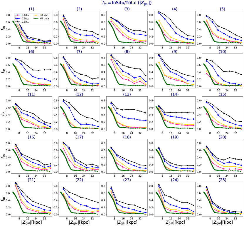
Figure 1: The |Z| profile depicts the fraction of insitu stars for different cutoffs, including (0.1, 0.2, 0.5) R_vir and 30 kpc, for a sample of 25 MW-like galaxies in the TNG50 simulation. In each panel, we have averaged over four different orientations for the Sun, located 8 kpc from the center in the disk plane, spanning $\pm{\hat{i}}$ and $\pm{\hat{j}}$. This averaging process helps reduce noise from various orientations. Overlaid on each panel, the solid green line represents the results from the H3 survey. Notably, there is a fair general agreement between the TNG50 results and the H3 survey, particularly for lower radial cuts. However, the level of agreement diminishes with increasing the threshold radius.

3.3 The insitu stars from TNG50 vs H3

Having outlined our general methodology for inferring the insitu stars from the TNG50 simulation, we proceed to compare our theoretical predictions with the actual observational results from the H3 survey.

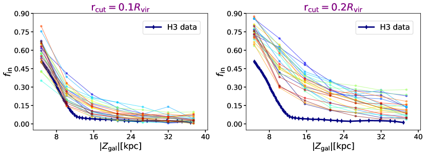
Figure 2: The |Z_gal| profile illustrates the fraction of insitu stars to the total number of stars derived from the TNG50 simulation using two different radial cutoffs: $r{\mathrm{cut}}=0.1R_{\mathrm{vir}}$ (left) and $r_{\mathrm{cut}}=0.2R_{\mathrm{vir}}$ (right). Each panel encompasses the entirety of TNG50 results, with the observational results from the H3 survey overlaid on each plot.

Figure 1 illustrates the |Z| profile of the fraction of insitu stars in various halos within our sample. Hereafter Z denotes the vertical height away from the disk. To establish the Z direction, we perform a coordinate transformation from the simulation frame to a coordinate system wherein the Z direction aligns with the total angular momentum of the stellar disk. We maintain flexibility in selecting the new X-Y directions within the disk plane. Since the H3 survey provides results in the Heliocentric coordinate system, with the Sun located approximately 8 kpc away from the center along the X direction, and given the absence of a real Sun in the TNG50 simulation, we repeat our analysis four times, placing the Sun in four arbitrary orientations along the ($\pm{\hat{i}}$ and $\pm{\hat{j}}$) directions. Subsequently, we average the final results obtained from the different orientations.

In each panel, solid lines of different colors [pink, blue, black] represent results using $r_{\mathrm{cut}}=[0.1,0.2,0.5]R_{\mathrm{vir}}$, respectively, while the solid yellow line depicts results using $r_{\mathrm{cut}}=30$ kpc. Additionally, the solid green line overlaid in each panel represents results from the H3 survey.

From the plot, several observations can be made:

$\bullet$ Increasing the radial cutoff does not drive the ratio of insitu stars to zero, indicating that insitu stars are present throughout most galaxies.

$\bullet$ The |Z| profile of the ratio of insitu stars varies among different galaxies. While some galaxies exhibit a significant decrease in $f_{\mathrm{in}}$ towards larger |Z|s, others display a smoother profile.

$\bullet$ Different galaxies exhibit varying sensitivity to different radial cutoffs. In some cases, increasing the radial cutoff notably enhances $f_{\mathrm{in}}$, whereas in others, it demonstrates less sensitivity.

$\bullet$ A constant cutoff of 30 kpc yields results similar to those obtained with a low radial cut of 0.1 $R_{\mathrm{vir}}$. This observation is intriguing as the curvature of the profile remains largely consistent across most cases, despite the former choice being a constant independent of individual galaxy specifics or the exact birth time of stars.

$\bullet$ In summary, a few galaxies [1, 11, 16, 18, 19, 23, 25] reasonably explain the trend in H3 results. Among these, only galaxies [1, 19, 25] match the observational results both in terms of the shape as well as the values of the insitu fraction regardless of the particular spatial cut for inferring the insitu fraction.

Figure 2 displays the Z profile of the fraction of insitu stars for all galaxies using two different radial cutoffs. The left panel corresponds to $r_{\mathrm{cut}}=0.1R_{\mathrm{vir}}$, while the right panel depicts $r_{\mathrm{cut}}=0.2R_{\mathrm{vir}}$. It is evident from the plot that increasing $r_{\mathrm{cut}}$ leads to a greater deviation of the inferred insitu fraction from the observational results obtained from the H3 survey. Conversely, at $r_{\mathrm{cut}}=0.1R_{\mathrm{vir}}$, most galaxies align well with the observational results. The lower cutoff appears more consistent with the constant cutoff utilized in previous literature (see for example Bonaca et al., 2017).

In the subsequent sections, we establish a connection between the deviation of the insitu fraction from the observational results and the merger history of different galaxies in our sample.

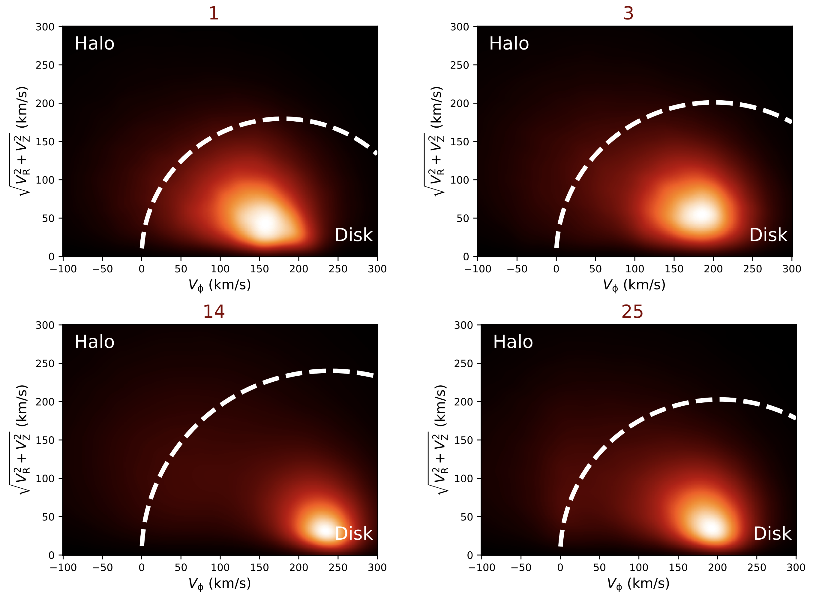
Figure 3: The Toomre diagram depicting the distribution of stars in four galaxies from our MW-like galaxy sample. The dashed line in each panel shows the boundary between halo-like and disk-like stars.

3.4 On the Origin of insitu stars

There have been various hypotheses proposed regarding the origin of insitu stars in galaxies. Gao et al. (2010); Griffen et al. (2018) suggested that the insitu component might originate from the collapse of cold gas, which is brought in from numerous gas-rich mergers. Conversely, they proposed that accreted stars could form from stellar sub-halos accreted onto the host galaxy. However, recent advancements, particularly through the analysis of Gaia DR1 and DR2, have significantly expanded our understanding beyond the solar neighborhood, providing insights into the galactic halo as well. Gaia data suggests that the insitu component of the galactic halo might be associated with a population of heated disk stars (see for example Bonaca et al., 2017; Haywood et al., 2018; Di Matteo et al., 2019; Belokurov et al., 2020; Sestito et al., 2019, and references therein). These observational findings align well with N-body analyses (see for instance Zolotov et al., 2010; Purcell et al., 2010; Font et al., 2011; Qu et al., 2011; McCarthy et al., 2012; Jean-Baptiste et al., 2017, and references therein).

The Toomre diagram is commonly employed to discern whether stars are part of the stellar halo or members of the stellar disk (see for example Bonaca et al., 2017; Di Matteo et al., 2020, and references therein). Motivated by these insights, we utilize the Toomre diagram to investigate the redshift evolution of stars in various orbits, encompassing both members of the stellar halo and the stellar disk. As a part of our analysis, we construct the Toomre diagram for a subset of galaxies in our MW-like galaxy sample at redshift zero. Subsequently, we leverage this diagram across the entire redshift evolution to classify stars into halo-like and disk-like components. Furthermore, we explore the role of galaxy mergers in influencing the evolution of the halo-like and disk-like components.

Figure 3 illustrates the Toomre diagram at redshift zero for a subset of 4 galaxies in our sample, with all stars being included in the plot. Each panel displays an overlaid dashed line representing the boundary between the stars in the disk-like and those on the halo-like orbits, defined as:

$$|V-V_{\mathrm{LSR}}|\geq V_{\mathrm{LSR}}~{},~{}~{}~{}~{}~{}~{}~{}~{}~{}\mathrm{Halo}$$

$$|V-V_{\mathrm{LSR}}|< V_{\mathrm{LSR}}~{},~{}~{}~{}~{}~{}~{}~{}~{}~{}\mathrm{Disk}$$ (1)

where we define $V_{\mathrm{LSR}}$ as the local standard of rest (LSR) speed, which is equivalent to the circular speed, $V_{\mathrm{cir}}(r)$, at the location of the Sun. Here, $V_{\mathrm{cir}}(r)\equiv\sqrt{GM_{\mathrm{tot}}(r)/r}$, where $M_{\mathrm{tot}}(r)$ refers to the total mass interior to distance $r$ including DM, star and gas particles. We consider the sun to be located at 8 kpc away from the galactic center at redshift zero. The x-axis of the Toomre diagram depicts the orbital speed along the stellar angular momentum, while the y-axis showcases the velocity orthogonal to the stellar disk angular momentum.

The selection of these galaxies is based on their insitu fraction profiles from Figure 1. Galaxies 1 and 25 exhibit profiles closely resembling the H3 observations, while galaxies 3 and 14 show progressively greater deviations from the observations as the spatial cut increases. Unexpectedly, galaxies 1 and 3 display more similar profiles, while galaxies 14 and 25 share greater similarities. Therefore the Toomre diagram may not be a sufficient metric to measure the similarities of simulated galaxies to the H3 observation. Moving forward we will use alternative metrics to quantify the observed deviations between the MW-like galaxies from the TNG50 simulations and the H3 observation.

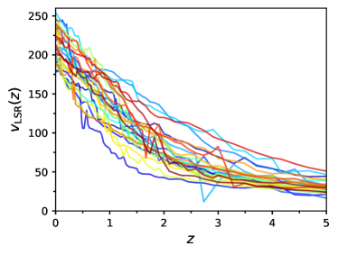
Figure 4: The redshift evolution of the local standard of rest (LSR) velocity for 25 MW-like galaxies in our sample. The velocity is in the unit of km/s.

As $V_{\mathrm{LSR}}$ speed is essential in the distinction between the halo-like and disk-like stars, in Figure 4 we present the redshift evolution of this quantity, defined as the circular speed $V_{\mathrm{cir}}$ evaluated at $r=A_{0}R_{\mathrm{h}}(z)$. Here, $R_{\mathrm{h}}(z)$ represents the redshift-dependent half-light radius, and $A_{0}$ is a constant determined such that $r=8$ kpc at redshift zero. Thus, we have $A_{0}=8/R_{\mathrm{h}}(z=0)$. The choice of 8 kpc ensures that the $V_{\mathrm{LSR}}$ is computed at the Sun’s location at present. While this choice is not unique, we expect the results to be relatively insensitive to it.

Figure 5: The redshift evolution of the fraction of the number of disk (represented by grey-circle) and halo (depicted by red-diamond) insitu stars between $r=17-23$ kpc to the total number of insitu stars at redshift zero with a cutoff of 0.2 $R_{\mathrm{vir}}$. Additionally, minor and major mergers are indicated by dashed-plum and solid-purple lines, respectively. The thresholds for minor and major mergers are set as 0.05-0.2 and above 0.2, respectively. It is seen that both the major and minor mergers change the slope of the evolution of the fraction of insitu stars.

Figure 5 illustrates the redshift evolution of the ratio of halo (denoted by diamond-red markers) and disk (represented by grey-circle markers) insitu stars as identified at redshift zero. While the insitu stars are defined using a spatial cut at 0.2 $R_{\mathrm{vir}}$, we only show the evolutionary trajectory of their number at $r=17-23$ kpc at zero redshifts, to the total number of insitu stars at redshift zero within the same radial range. We have chosen this range, $r=17-23$ kpc, as according to Figure 1, the insitu stellar fraction diminishes significantly in this interval. Furthermore, to simplify delivering the picture, we only present the results for a case with the Sun located at 8 kpc in the +X direction.

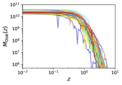
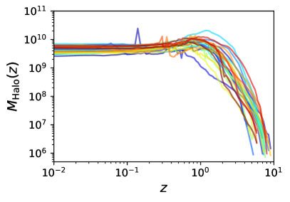
Figure 6: The redshift evolution of the total mass of the disk insitu stars (left panel) and halo insitu stars (right panel), defined with a spatial cutoff of 0.2 $R_{\mathrm{vir}}$.

For each galaxy, we start with the total number of ‘observed’ insitu stars from the H3 survey and trace them back in time. At each redshift, we compute the $V_{\mathrm{LSR}}$ and categorize the stars into halo (diamond-red) and disk (grey-circle) components. Additionally, major mergers are depicted by solid-purple lines, while minor mergers are represented by dashed-plum lines.

The two ratios are complementary as expected. It is evident that stars on disk orbits begin with a negligible fraction at high redshifts and gradually increase in their percentage towards lower redshifts. Ultimately, at redshift zero, the insitu stellar fraction is predominantly dominated by stars in disk-like orbits, which aligns with the predominant stellar disk characteristic of MW-like galaxies. Galaxy mergers play a role in altering the growth/decline slope for both halo and disk stars.

Figure 6 illustrates the redshift evolution of the insitu stellar mass in disk orbits (left panel) and halo orbits (right panel). The original insitu stars are traced back in time, and in each snapshot, the stellar mass in the disk and halo orbits is inferred. It is observed that throughout the galaxy’s evolution, the total stellar mass in both disk and halo orbits increases, with the final mass in disk stars being dominant over their values in halo orbits.

3.5 Redshift Evolution of R_vir and SFR

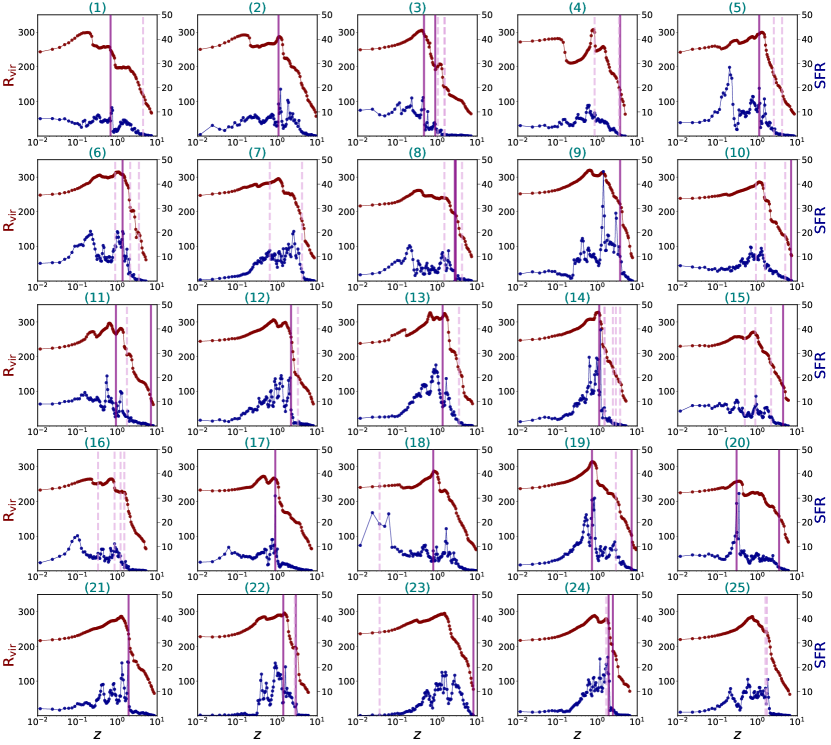
Figure 7: Redshift evolution of the comoving virial radius (R${\mathrm{vir}}$) (left) and the star formation rate (SFR) (right) for our sample of MW-like galaxies. Vertical solid lines (purple) indicate major mergers, while dashed lines (plum) represent minor mergers. It is observed that both R${\mathrm{vir}}$ and SFR are enhanced during merger events.

With the merger history of the first progenitor elucidated, we now delve into the redshift evolution of two key parameters in our analysis: the comoving virial radius $R_{\mathrm{vir}}$ and the star formation rate (SFR). The comoving virial radius is pertinent as it influences the radial cutoff used to infer the insitu stars at each redshift. On the other hand, the SFR is linked to the insitu stellar budget at any given time. Both of these quantities are impacted by merger events.

Figure 7 presents the redshift evolution of $R_{\mathrm{vir}}$ and the SFR for our entire MW-like sample. In each plot, the time of major mergers is indicated by a solid purple line, while minor mergers are represented by dashed plum lines.

Throughout the galaxy’s evolutionary trajectory, instances arise where either or both $R_{\mathrm{vir}}$ and SFR change their amplitude and slope. While there are various reasons for these slope variations, e.g. owing to galaxy-galaxy mergers, due to pseudo-evolution owing to cosmic evolution, below we mainly focus on their impact on the evolution of insitu star fraction. More specifically, we embark on an analysis to explore the correlation between the evolution of these quantities and the deviation between the insitu fraction inferred from the TNG50 simulations and the H3 survey.

3.5.1 Quantitative comparison between TNG50 and H3 results

As already mentioned above, our main goal is to make a comparison between the scale dependence of the insitu halo stars from the H3 survey and the TNG simulation. Since the H3 survey gives the insitu halo stars at a few different scale heights from the disk plane, to make the comparison more robust, we should present an effective quantity that encodes both the difference between the fraction of insitu stars between the simulation and data as well as the difference between their (spatial) slope. In addition, since the theoretically inferred insitu fraction depends on the actual cutoff, we may want to try different deviations at the level of 0.1$R_{\rm{vir}}$, 0.2$R_{\rm{vir}}$, and 0.5$R_{\rm{vir}}$. This suggests the following effective quantity at different levels:

$$\Delta f^{j}_{\mathrm{eff}}\equiv ~{}\bigg{|}\frac{\sum_{i=1}^{\mathrm{N_{1}}}\bigg{(}f^{j}_{\mathrm{in}}(i)-f_{\mathrm{H3}}(i)\bigg{)}}{2\mathrm{N_{1}}}\bigg{|}+\bigg{|}\frac{\sum_{i=1}^{\mathrm{N}}\bigg{(}f^{\prime j}_{\mathrm{in}}(i)-f^{\prime}_{\mathrm{H3}}(i)\bigg{)}}{\mathrm{N_{2}}}\bigg{|}$$

$$\equiv ~{}\Delta f^{j}_{\mathrm{Amp}}+\Delta f^{j}_{\mathrm{Slope}}~{}~{}~{},~{}~{}~{}j=(0.1,0.2,0.5).$$ (2)

where to compare between the insitu star fraction from the TNG50 and the H3 observation we make some bins along the scale height. To define these spatial bins, we tried two different metrics. One is the regular bins covering the scale heights from 3-20 kpc and the other is focusing on larger distances (between 17-20kpc) for the amplitude deviation, with the total number of bins with the total bin numbers $\mathrm{N_{1}}=23$, and on smaller distances (between 5-7.5 kpc) for its derivatives, with the total bin numbers $\mathrm{N_{1}}=10$. As it turns out, the second metric gives us better correlation matrix coefficients. We therefore choose this metric in our following analysis. In Eq. 3.5.1, $i$ refers to the indices associated with these bins. Using $\Delta f^{j}_{\mathrm{eff}}$, we can associate one number to every galaxy and use it as a proxy to judge how close the simulated galaxy is to the observations. Another advantage of this metric is that we can make an automated way to accurately infer the proximity between the theory and H3 observation.

Below, we extensively make use of $\Delta f^{j}_{\mathrm{eff}}$ when we connect the above deviations to the merger history and the actual properties of individual halos. Our goal is to find some possible correlations between how small/large is $\Delta f^{j}_{\mathrm{eff}}$ and the closeness of different MW-like galaxies chosen from the TNG and the actual MW from the H3.

4 Exploring different drivers for the insitu stars

Having quantified the effective deviation in the insitu stellar fraction between the TNG50 and H3 survey datasets, our objective is to establish a correlation between this metric and the key parameter characterizing each galaxy, as well as its assembly history. This analysis involves two main categories of parameters: internal drivers and external factors. Below, we investigate the influence of these drivers and their association with the $\Delta f^{j}_{\mathrm{eff}},j=(0.1,0.2,0.5)$ quantity derived from Eq. 3.5.1.

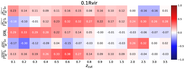
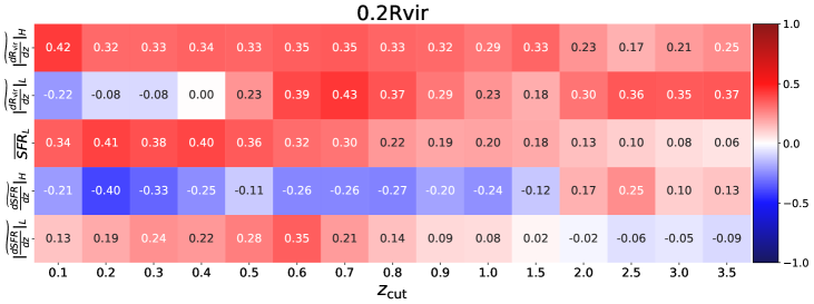
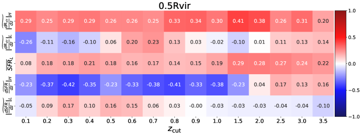
Figure 8: The correlation coefficient of $\widetilde{|\frac{dR_{\mathrm{vir}}}{dz}|}_{H}$, $\widetilde{|\frac{dR_{\mathrm{vir}}}{dz}|}_{L}$, $\overline{\mathrm{SFR}}_{L}$, $\widetilde{\frac{d\mathrm{SFR}}{dz}}|_{H}$ and $\widetilde{|\frac{d\mathrm{SFR}}{dz}|}_{L}$ with $\Delta f^{j}_{\mathrm{eff}}$. Different matrices from top to bottom correspond to various spatial cuts of $j=(0.1,0.2,0.5)$, respectively.

4.1 Internal drivers for the insitu fraction

As discussed in Section 3.5, $R_{\mathrm{vir}}$ and the SFR are fundamental internal parameters with direct implications for galaxy evolution. Building upon this insight, we investigate the correlation matrix between these parameters and Eq. 3.5.1. Given the evolutionary nature of these internal drivers over a galaxy’s lifespan, we segment the data into redshift bins to analyze their significance at different epochs. Specifically, we compute the mean, median, and slope of these parameters using two distinct approaches: either from an initial redshift to $z_{\mathrm{cut}}$ (referred to as $H$), or from $z_{\mathrm{cut}}$ to redshift zero (named as $L$). Subsequently, we assess the correlation between these metrics and $\Delta f^{j}_{\mathrm{eff}},j=(0.1,0.2,0.5)$ derived from Eq. 3.5.1.

Figure 8 illustrates the correlation coefficient matrix for both the $H$ and $L$ redshift segments across varying $z_{\mathrm{cut}}$ values. Each row represents a spatial cut, progressively increasing from $0.1R_{\mathrm{vir}}$ to $0.5R_{\mathrm{vir}}$. While there are discernible variations in correlation coefficients between the smallest ($0.1R_{\mathrm{vir}}$) and largest ($0.5R_{\mathrm{vir}}$) cuts, overall trends, including magnitude and sign, remain consistent. The median and mean of the X quantity are denoted by $\tilde{\mathrm{X}}$ and $\overline{\mathrm{X}}$, respectively.

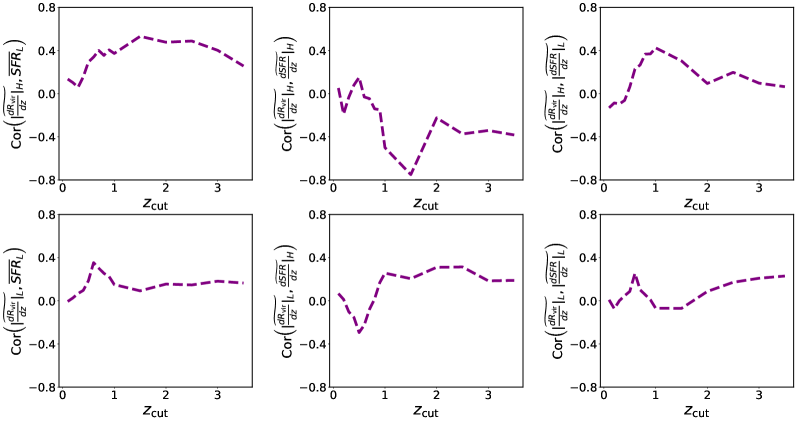
Figure 9: The cross-correlation coefficient between different internal metrics. In top/bottom row, from left to right, we present the correlation of $\widetilde{\frac{dR_{\mathrm{vir}}}{dz}}|_{H}$/$\widetilde{\frac{dR_{\mathrm{vir}}}{dz}}|_{L}$ with $\overline{SFR}_{L}$, $\widetilde{\frac{dSFR}{dz}}|_{H}$ and $\widetilde{\frac{dSFR}{dz}}|_{L}$, respectively.

Within each correlation matrix, the importance of different metrics fluctuates across $z_{\mathrm{cut}}$ values, underscoring the significance of both amplitude and slope in delineating deviations between theory and observation. Notably, the mean value of the SFR demonstrates a significant correlation, while the slope of $R_{\mathrm{vir}}$ holds greater significance than its absolute value. Additionally, the median slope for both the SFR and $R_{\mathrm{vir}}$ emerges as more influential than their mean counterparts, suggesting that gradual variations in these quantities carry more weight than outliers. Moreover, our expanded metric, incorporating both mean and median values alongside absolute valued parameters, unveiled intriguing correlations. Notably, for $\frac{dR_{\mathrm{vir}}}{dz}$, absolute valued medians exhibited stronger correlations, contrasting with the SFR and $\frac{d\mathrm{SFR}}{dz}|_{H}$, where mean and median absolute values yielded weaker correlations. This discovery prompted a flexible approach, alternating between normal and absolute values for different parameters. As expected, the handling of negative values revealed disparities in the correlation coefficient sign between normal and absolute valued quantities, highlighting the nuanced nature of these relationships.

It is evident that in most cases, $\widetilde{|\frac{dR_{\mathrm{vir}}}{dz}|}_{H}$ is positively correlated with $\Delta f^{j}_{\mathrm{eff}},j=(0.1,0.2,0.5)$. To elucidate the underlying reason for this positive correlation, we delve deeper into Figure 7, where it becomes apparent that $R_{\mathrm{vir}}$ undergoes two distinct evolutionary phases: a growth phase followed by a diminishment phase. The transition point from the former to the latter phase varies across different galaxies. An earlier rapid growth expands the boundaries of $R_{\mathrm{vir}}$ to larger distances, consequently increasing the fraction of insitu stars and thereby elevating the value of $\Delta f^{j}_{\mathrm{eff}},j=(0.1,0.2,0.5)$. Moreover, Figure 8 suggests that for a very early redshift cut, i.e., the higher values of $z_{\mathrm{cut}}$, larger spatial cuts are more correlated than the lower values. We posit that this phenomenon is associated with the inclusion of the transitional phase from an increasing to diminishing evolutionary phase of $R_{\mathrm{vir}}$.

At lower values of $z_{\mathrm{cut}}$, $\widetilde{|\frac{dR_{\mathrm{vir}}}{dz}|}_{L}$ is anti-correlated with $\Delta f^{j}_{\mathrm{eff}},j=(0.1,0.2,0.5)$, indicating that as $R_{\mathrm{vir}}$ diminishes, the spatial boundaries contract, resulting in a more concentrated distribution of stars and thus lower values of $\Delta f^{j}_{\mathrm{eff}},j=(0.1,0.2,0.5)$. Conversely, at higher values of $z_{\mathrm{cut}}$, this anti-correlation transitions to a positive correlation. We interpret this shift as a consequence of changes in the slope of $R_{\mathrm{vir}}$ corresponding to increasing $z_{\mathrm{cut}}$.

Figure 8 illustrates a positive correlation between $\overline{\mathrm{SFR}}_{L}$ and $\Delta f^{j}_{\mathrm{eff}},j=(0.1,0.2,0.5)$. This correlation signifies the potential for higher $\overline{\mathrm{SFR}}_{L}$ values to stimulate star formation across various regions of galaxies. Notably, the strength of this correlation fluctuates with $z_{\mathrm{cut}}$: stronger correlations are evident at smaller spatial cuts for lower $z_{\mathrm{cut}}$ values, while stronger correlations occur at larger spatial cuts for higher $z_{\mathrm{cut}}$ values. We postulate that this behavior can be attributed to the evolutionary dynamics of galaxies. After disk formation, stars tend to concentrate closer to the center, leading to stronger correlations for smaller spatial cuts. Conversely, as redshift increases, stars formed at larger distances become more influential, migrating towards the central regions of galaxies and reinforcing correlations at larger spatial cuts. The lower correlation observed for lower spatial cuts may be attributed to the fact that stars migrate closer to the center, diminishing their contribution to $\Delta f^{j}_{\mathrm{eff}},j=(0.1,0.2,0.5)$.

The behavior of $\widetilde{\frac{d\mathrm{SFR}}{dz}}|_{H}$ closely mirrors that of $\widetilde{|\frac{dR{\mathrm{vir}}}{dz}|}_{H}$, with one notable exception: to enhance the correlation level, we omit the median of the absolute value of $\widetilde{\frac{d\mathrm{SFR}}{dz}}|_{H}$, resulting in a reversal of the correlation coefficient’s sign. This trend is also observed in $\widetilde{|\frac{d\mathrm{SFR}}{dz}|}_{L}$, where the median is computed over the absolute value.

In summary, the correlation coefficient structure exhibits remarkable consistency between $R_{\mathrm{vir}}$ and SFR. In most cases, the median of the absolute valued derivative shows a positive correlation with $\Delta f^{j}_{\mathrm{eff}},j=(0.1,0.2,0.5)$, underscoring the role of enhancements in these values in amplifying the insitu stellar fraction across galaxies.

Figure 9 showcases the cross-correlation between various internal metrics and $z_{\mathrm{cut}}$. The top and bottom rows correspond to $\widetilde{\frac{dR_{\mathrm{vir}}}{dz}}|_{H}$ and $\widetilde{\frac{dR{\mathrm{vir}}}{dz}}|_{L}$, respectively, in conjunction with stellar-driven metrics. Within each row, from left to right, we demonstrate the correlation of $\widetilde{|\frac{dR{\mathrm{vir}}}{dz}|}_{i=(H,L)}$ with $\overline{\mathrm{SFR}}_{L}$, $\widetilde{\frac{d\mathrm{SFR}}{dz}}|_{H}$, and $\widetilde{|\frac{d\mathrm{SFR}}{dz}|}_{L}$, respectively. The presence of non-zero cross-correlations between different components suggests their shared contributions to $\Delta f^{j}_{\mathrm{eff}},j=(0.1,0.2,0.5)$.

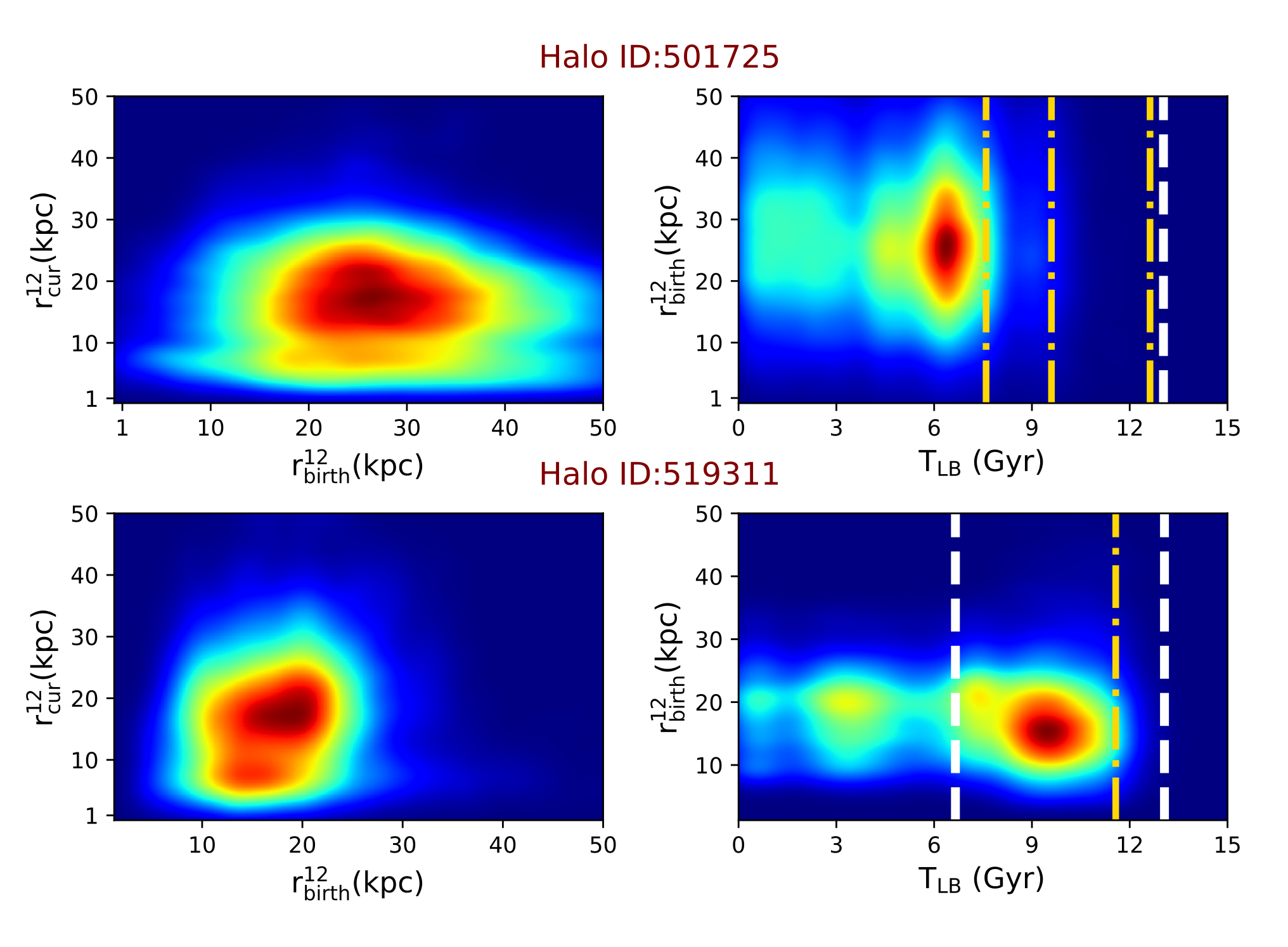
Figure 10: Rows present the birth location vs the current location (left panels) as well as the look-back time (T_LB) vs the birth location (right panels) of the insitu stars located between the 0.1 R_vir and 0.2 R_vir in two galaxies of the sample analyzed in this work. The dotted-dashed-gold and dashed-white lines refer to the minor and major mergers, respectively. Both minor and major mergers are important in elevating star formation and producing insitu stars. In addition, insitu stars get closer to the center after their birth.

4.2 External drivers for the insitu fraction

During the evolutionary trajectory of galaxies, numerous external events, including mergers and disruptions, play pivotal roles in shaping their dynamics. These events significantly influence star formation rates and redistribute stars within galaxies. Our objective here is to investigate how galaxy mergers impact the distribution of insitu stars.

Figure 10 illustrates the influence of galaxy mergers on the creation and distribution of insitu stars in two galaxies (depicted in the top and bottom rows) of our galaxy sample. The left panels depict the birth location versus the current location, while the right panels display the look-back time (TLB) versus the birth location of the insitu stars located between 0.1-0.2 $R_{\mathrm{vir}}$. The dotted-dashed-gold and dashed-white lines denote minor and major mergers, respectively. Both minor and major mergers play a significant role in enhancing star formation and generating insitu stars. Moreover, the analysis suggests that insitu stars tend to migrate closer to the center following their birth. Motivated by this, in the following, we compile a comprehensive list of potentially influential parameters and analyze their correlation coefficients with $\Delta f^{j}_{\mathrm{eff}},j=(0.1,0.2,0.5)$. We provide detailed definitions of each parameter and elucidate their respective contributions to the observed deviations between the TNG50 and H3 datasets.

$\bullet$ Effective mass-ratio: One of the crucial parameters significantly influencing $\Delta f^{j}_{\mathrm{eff}}$, $j=(0.1,0.2,0.5)$, is the mass-ratio of galaxy mergers. Motivated by this insight, we introduce a metric termed the effective mass-ratio of galaxy mergers, $\overline{\mathrm{MR}}$, which encompasses both stellar mass and star-forming gas mass-ratios. While the role of the stellar mass-ratio, between first and second progenitors, is relatively well-understood, the influence of star-forming gas warrants further investigation. We posit that a gas-rich galaxy merger collectively enhances star formation. Consequently, we incorporate this additional contribution into our metric and observe a consistent correlation coefficient across all cases.

For each of these contributions, we compute the average mass-ratio above a specified threshold, denoted as $f_{\mathrm{MM}}$, after a designated redshift threshold. In subsequent analyses, we explore the impact of two values for the mass-ratio threshold, specifically $f_{\mathrm{MM}}=(0.05,0.2)$. Additionally, through exploratory investigations, we determine that a redshift threshold of $z\leq 4$ effectively provides a better correlation, as the majority of galaxy evolution occurs below this threshold. Furthermore, it is observed that this threshold is consistent with the mass-weighted mass-ratio as defined in Appendix A.

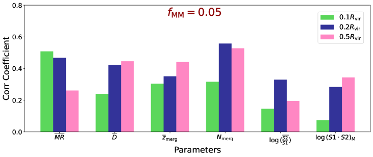
Figure 11: The correlation coefficient between parameters associated with galaxy mergers and $\Delta f^{j}_{\mathrm{eff}},j=(0.1,0.2,0.5)$. The top row presents the correlation coefficient for the galaxy mergers above the effective mass-ratio 0.05, while the bottom row depicts the correlation coefficient for mergers with mass-ratio above 0.2.

$\overline{\mathrm{MR}}$ is defined as:

$$\overline{\mathrm{MR}}=\frac{1}{N}\sum_{i}^{N}\left(\mathrm{MR}_{*}+\mathrm{MR}_{g}\right)_{i},$$ (3)

where the summation index $i$ is over the total number of the mergers with the mass-ration above $f_{\mathrm{MM}}$. In each merger event, we identify the first and the second progenitors with $M^{f}_{i}$ and $M^{s}_{i}$, respectively. Furthermore, $\mathrm{MR}_{j}\equiv M^{s}_{i}/M^{f}_{i}$, $j=*$, and $j=g$ denote the mass-ratio of stars to star-forming gas, respectively.

$\bullet$ Mean distance: The second crucial parameter, correlated with $\Delta f^{j}_{\mathrm{eff}},j=(0.1,0.2,0.5)$, pertains to the impact parameter in galaxy mergers. In the event of a galaxy merger, the distance between the first and second galaxy significantly influences the redistribution of stars. Our analysis involves computing the average distance, hereafter referred to as $\overline{D}$, between the first and second galaxy of any galaxy mergers with mass-ratio above $f_{\mathrm{MM}}$ happening below the $z\leq 4$. The distance is inferred at the time when the second progenitor gets to the peak of its mass. Since we do not have enough time resolution in the cosmological simulations, it is common to approximate this snapshot, or its subsequent snapshot, at the time of the merger.

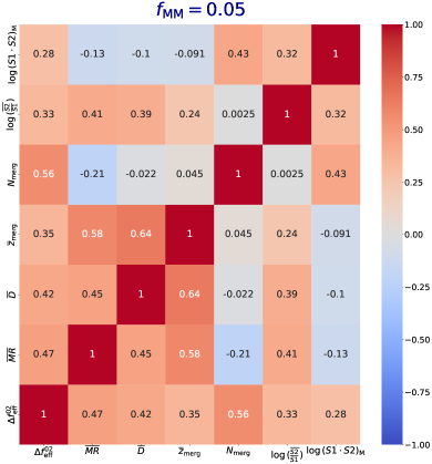
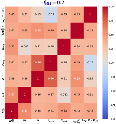
Figure 12: Depiction of the correlation coefficient matrix illustrating the relationships between external parameters and $\Delta f^{j}_{\mathrm{eff}}$, as well as among themselves. The left panel corresponds to $f_{\mathrm{MM}}=0.05$, while the right panel illustrates the case with $f_{\mathrm{MM}}=0.2$.

$\bullet$ Effective redshift: The third critical parameter influencing $\Delta f^{j}_{\mathrm{eff}},j=(0.1,0.2,0.5)$, is the timing of galaxy mergers. The occurrence of a galaxy merger during the primary epoch of galaxy evolution may exert a more pronounced effect on the stellar profile compared to mergers happening later. We establish an effective redshift of mergers, denoted as $z_{\mathrm{eff}}$, for mergers transpiring below $z\leq 4$ and surpassing a certain merger fraction threshold $f_{\mathrm{MM}}$. This effective redshift is calculated as $z_{\mathrm{eff}}=(1/N)\sum_{i}^{N}z_{i}$, where $N$ represents the total number of galaxy mergers.

$\bullet$ Number of mergers: The fourth pivotal parameter is the total number of mergers with mass-ratios exceeding $f_{\mathrm{MM}}$ occurring below $z\leq 4$. We denote this quantity as $N_{\mathrm{merg}}$ and explore its correlation with $\Delta f^{j}_{\mathrm{eff}},j=(0.1,0.2,0.5)$.

$\bullet$ Mean spin ratio: The fifth pivotal parameter associated with $\Delta f^{j}_{\mathrm{eff}},j=(0.1,0.2,0.5)$, is the spin ratio between the first and second progenitors at the moment of a merger. We define the average value of this spin ratio, incorporating all galaxy mergers with mass-ratios exceeding $f_{\mathrm{MM}}$ occurring below $z\leq 4$ throughout the merger history of galaxies, and denote this quantity as $\overline{\left(\frac{S2}{S1}\right)}$. Our investigation revealed that taking the logarithm of this quantity yields a stronger correlation. Therefore, we employ $\log{(\overline{\frac{S2}{S1}})}$ when computing the correlation coefficients.

$\bullet$ Maximum spin alignment: The final critical parameter associated with $\Delta f^{j}_{\mathrm{eff}},j=(0.1,0.2,0.5)$, is the spin alignment between the first and second progenitors. We differentiate between the impact of face-on and edge-on galaxy mergers on the redistribution of stars across galaxies. Our investigation has demonstrated that the maximum alignment, derived from a subset of galaxy mergers meeting the aforementioned criteria, yields a stronger correlation coefficient. Furthermore, it has been observed that the logarithm of this quantity provides an even higher correlation. We define this parameter as $\log{(S1\cdot S2)_{\mathrm{M}}}$.

4.2.1 Corr(External driver, $\Delta f^{j}_{\mathrm{eff}}$)

Figure 11 illustrates the correlation function between individual external parameters and $\Delta f^{j}_{\mathrm{eff}}$. The first and second rows present the correlation coefficients for $f_{\mathrm{MM}}=0.05$ and $f_{\mathrm{MM}}=0.2$, respectively. Within each row, different colors represent distinct spatial cuts: green, blue, and pink correspond to 0.1$R_{\mathrm{vir}}$, 0.2$R_{\mathrm{vir}}$, and 0.5$R_{\mathrm{vir}}$, respectively.

From the plot, it is evident that all external drivers are positively correlated with $\Delta f^{j}_{\mathrm{eff}}$, although the strength of correlation coefficients varies across different spatial cuts and mass-ratio merger thresholds. While it is anticipated that higher values of $\overline{\mathrm{MR}}$ and $N_{\mathrm{merg}}$ result in larger $\Delta f^{j}_{\mathrm{eff}}$, it is less intuitive how much a larger $\overline{D}$ and $z_{\mathrm{eff}}$ positively correlate with $\Delta f^{j}_{\mathrm{eff}}$. In the former case, we propose that galaxy mergers with larger impact parameters extract stars from individual galaxies as well as leave star-forming gas in larger distances, causing them to become more extended. Regarding the latter case, our analysis suggests that having galaxy mergers at higher redshifts, albeit below $z=4$, is crucial for transporting gas to the outer regions of galaxies, thus facilitating star formation at subsequent redshifts.

The highest correlation coefficient at $f_{\mathrm{MM}}=0.05$ is attributed to $N_{\mathrm{merg}}$, suggesting its strongest association with $\Delta f^{j}_{\mathrm{eff}}$. Nevertheless, both $\overline{\mathrm{MR}}$ and $z_{\mathrm{eff}}$ also exhibit significant importance.

At $f_{\mathrm{MM}}=0.05$, the lowest correlation coefficient is linked to the spin-driven quantities, although this changes at $f_{\mathrm{MM}}=0.2$. At this level, the correlation coefficients for all quantities at 0.2$R_{\mathrm{vir}}$ increase, while some of them decrease for 0.1$R_{\mathrm{vir}}$. This intricate pattern underscores the complexities involved in shaping the stellar distribution across galaxies and highlights the intricacies of galaxy evolution.

While Figure 11 illustrates the significance of individual parameters in influencing $\Delta f^{j}_{\mathrm{eff}}$, it does not quantify the extent to which these external drivers may overlap or exhibit degeneracy in their correlation coefficients. To quantify potential levels of degeneracy between different external drivers, we proceed by computing the cross-correlation between these quantities.

4.2.2 Corr(External driver, External driver)

Figure 12 depicts the correlation coefficient matrix, illustrating the relationships between external parameters and $\Delta f^{j}_{\mathrm{eff}}$, as well as among themselves. The left panel corresponds to $f_{\mathrm{MM}}=0.05$, while the right panel illustrates the case with $f_{\mathrm{MM}}=0.2$.

Positive and negative cross-correlations are reported, although the statistical significance of negative correlations is notably smaller than that of positive cases. Hence, our focus lies solely on positive correlations. Notably, $\overline{\mathrm{MR}}$ exhibits strong correlations with $\overline{D}$, $z_{\mathrm{eff}}$, and $\log{(\overline{\frac{S2}{S1}})}$. This is attributed to higher mass-ratios potentially exerting stronger impacts on average impact parameter values. Additionally, the positive correlation with $z_{\mathrm{eff}}$ suggests that mergers with higher mass-ratios may tend to occur at higher redshifts. Furthermore, a positive correlation with $\log{(\overline{\frac{S2}{S1}})}$ indicates that galaxy mergers with higher mass-ratios may also correspond to higher spin fractions, although alignment is not necessarily guaranteed.

$\overline{D}$ is correlated with $z_{\mathrm{eff}}$, hinting that galaxy mergers at higher redshifts may involve larger impact parameters. While this observation is intriguing, further justification will be pursued in future work with a larger galaxy sample.

Additionally, the number of mergers shows a positive correlation with $\log{(S1\cdot S2)_{\mathrm{M}}}$, suggesting that a larger number of galaxy mergers statistically facilitates the occurrence of more aligned systems. Moreover, there are positive correlations between $\log{(\overline{\frac{S2}{S1}})}$ and $\log{(S1\cdot S2)_{\mathrm{M}}}$, indicating that, on average, systems with higher spin fractions may exhibit higher alignments.

These observations reveal overlapping effects between key drivers, ultimately enhancing their correlation coefficients with $\Delta f^{j}_{\mathrm{eff}}$. Consequently, it is imperative to be cautious when listing the key external parameters, as their impacts may be lower due to the aforementioned degeneracy with other parameters.

5 Conclusions

In this study, we conducted a comprehensive analysis of the distribution of insitu stars from a sample of Milky Way-like galaxies from the TNG50 simulation. The identification process relied solely on the stellar birth location within the first progenitor throughout the galaxy’s evolution. We investigated the effects of various spatial cuts, including 30 kpc, 0.1$R_{\mathrm{vir}}$, 0.2$R_{\mathrm{vir}}$, and 0.5$R_{\mathrm{vir}}$, on the profile distribution of insitu stars, along with an additional spatial cut akin to the heliocentric coordinate of the H3 survey. Subsequently, we compared the scale height distribution of insitu stars from TNG50 with the latest observational outcomes from the H3 survey, identifying the impact of different internal and external parameters in inducing deviations between theory and observation.

Below, we summarize some of the key steps and highlight a few takeaways from this exploratory investigation.

1. We conducted an analysis to determine the correlation coefficient between $\Delta f^{j}_{\mathrm{eff}}$ from Eq. 3.5.1 and internal drivers, such as the mean/median of the amplitude and derivatives $R_{\mathrm{vir}}$ and the SFR over various time intervals. These intervals encompassed either the period from an initial redshift to $z_{\mathrm{cut}}$ or from $z_{\mathrm{cut}}$ to redshift zero.

2. The observed positive correlation between $\widetilde{|\frac{dR_{\mathrm{vir}}}{dz}|}_{H}$ and $\Delta f^{j}_{\mathrm{eff}}$ in Figure 8, particularly at higher $z_{\mathrm{cut}}$ values, indicates that the expansion of $R_{\mathrm{vir}}$ encompasses more insitu stars, leading to an increase in $\Delta f^{j}_{\mathrm{eff}}$.

3. At lower $z_{\mathrm{cut}}$ values, Figure 8 implies that $\widetilde{|\frac{dR_{\mathrm{vir}}}{dz}|}_{L}$ inversely correlates with $\Delta f^{j}_{\mathrm{eff}}$, indicating a contraction of spatial boundaries with decreasing $R_{\mathrm{vir}}$ and lower $\Delta f^{j}_{\mathrm{eff}}$ values. Conversely, at higher $z_{\mathrm{cut}}$, this correlation shifts to a positive correlation, possibly due to changes in $R_{\mathrm{vir}}$ slope with increasing $z_{\mathrm{cut}}$.

4. Figure 8 illustrates varying correlations between $\overline{\mathrm{SFR}}_{L}$ and $\Delta f^{j}_{\mathrm{eff}}$ across different $z_{\mathrm{cut}}$ values. Stronger correlations are evident at smaller spatial cuts for lower $z_{\mathrm{cut}}$, whereas they occur at larger spatial cuts for higher $z_{\mathrm{cut}}$. This suggests an influence of galaxy evolution dynamics, with stars tending to concentrate closer to the center after disk formation, reinforcing correlations for smaller spatial cuts. Conversely, stars formed at larger distances become more influential with increasing redshift, strengthening correlations at larger spatial cuts.

5. The non-zero cross-correlation observed among different internal drivers, as depicted in Figure 9, indicates their shared influence on $\Delta f^{j}_{\mathrm{eff}}$.

6. Our analysis, as depicted in Figure 10, emphasizes the considerable impact of mergers on star formation. Additionally, it reveals a consistent pattern of insitu stars migrating towards the galactic center post-formation.

7. Moreover, our analysis revealed six key parameters linked to galaxy mergers that notably influence the creation and distribution of insitu stars. These parameters include the merger effective mass-ratio, mean distance between galaxy mergers, effective redshift of mergers, number of mergers, mean spin ratio of galaxy mergers, and maximum spin alignments from galaxy mergers.

8. The correlation analysis, presented in Figure 11, reveals positive correlations between all external drivers and $\Delta f^{j}_{\mathrm{eff}}$, albeit with varying strengths across different spatial cuts and mass-ratio merger thresholds. Higher values of $\overline{\mathrm{MR}}$ and $N_{\mathrm{merg}}$ are expected to increase $\Delta f^{j}_{\mathrm{eff}}$. However, the impact of larger $\overline{D}$ and $z_{\mathrm{eff}}$ on $\Delta f^{j}_{\mathrm{eff}}$ is less straightforward. Larger impact parameters in galaxy mergers pushes stars to larger distances, resulting in extended distributions. Moreover, galaxy mergers at higher redshifts, below $z=4$, facilitate gas transportation to the outer regions of galaxies, promoting subsequent star formation.

9. Our analysis, illustrated in Figure 12, reveals positive cross-correlations between different external parameters, suggesting some degree of degeneracy in influencing $\Delta f^{j}_{\mathrm{eff}}$. Notably, a strong correlation is observed between $\overline{\mathrm{MR}}$ and $\overline{D}$, $z_{\mathrm{eff}}$, and $\log{(\overline{\frac{S2}{S1}})}$. Additionally, $\overline{D}$ is correlated with $z_{\mathrm{eff}}$. Lastly, $N_{\mathrm{merg}}$ exhibits a positive correlation with $\log{(S1\cdot S2)_{\mathrm{M}}}$, while $\log{(S1\cdot S2)_{\mathrm{M}}}$ is also correlated with $\log{(S1\cdot S2)_{\mathrm{M}}}$.

10. While the significant correlations observed between external parameters and $\Delta f^{j}_{\mathrm{eff}}$, as well as among themselves, are intriguing, it is important to note that the statistical reliability of some correlation coefficients may be impacted by the small sample size. To address this concern, we employed a Random Forest Regression method in Appendix B to assess the generalizability of these results using a machine learning approach. The results, depicted in Figure 13, indicate that the correlation strengths between these parameters and $\Delta f^{j}_{\mathrm{eff}}$ remain relatively consistent after conducting the Random Forest Regression.

Future Directions

In future studies, we aim to expand our galaxy sample size to a bigger sample to further validate our conclusions. Additionally, we plan to investigate the influence of mergers on individual galaxy spins and star formation by utilizing isolated galaxy merger simulations and zoom-in simulations with increased spatial and temporal resolution. Finally, while in the current study, we mainly followed a theoretically driven approach to identify the insitu stars based on a spatial cut, in a follow-up work we plan to extend this fundamental study by taking a more chemically oriented approach in defining the insitu stars. While our initial investigations demonstrated that the results are not heavily sensitive to this choice, it is worth checking how much this conclusion might be changed if we use an alternative cosmological simulation with a better-defined stellar population.

Data Availability

Data directly associated with this manuscript and its figures can be provided upon reasonable request from the corresponding author. The IllustrisTNG and TNG50 simulations are publicly available and accessible at www.tng-project.org/data (Nelson et al., 2019b).

Appendix A Effective mass-ratio

As already stated in Eq. 3, the mass-ratio is defined by combining the stellar mass-ratio and star-forming gas ratio. While this quantity is closely connected to the other external parameters, as well as $\Delta f^{j}_{\mathrm{eff}}$, we chose a redshift threshold of $z\leq 4$ for including mergers in the system. This threshold was chosen to ensure that we consider enough prior galaxy evolution while also incorporating the main evolution of galaxies into account. To verify the justification of this threshold, we extend beyond the former definition and define a mass-weighted merger mass-ratio without requiring a specific redshift threshold. More explicitly, for each merger event, in the numerator, we add an extra factor of the mass of the second progenitor. This is given as:

$$\mathrm{MR}_{\mathrm{eff}}\equiv\frac{\sum_{i=1}^{N}\left(\frac{\left(M^{s}_{*}\right)^{2}}{M^{f}_{*}}\right)_{i}}{\sum_{i=1}^{N}(M^{s}_{*})_{i}}+\frac{\sum_{i=1}^{N}\left(\frac{\left(M^{s}_{g}\right)^{2}}{M^{f}_{g}}\right)_{i}}{\sum_{i=1}^{N}(M^{s}_{g})_{i}}.$$ (A1)

where $M^{j}_{*},j=(f,s)$ refers to the stellar mass in the first and second progenitors, while $M^{j}_{g},j=(f,s)$ describes the gaseous mass in the first/second progenitor, respectively. Our analysis demonstrated that the correlation level between this new mass-ratio and $\Delta f^{j}_{\mathrm{eff}}$ is compatible with that of $\overline{\mathrm{MR}}$. Consequently, we focus exclusively on using the former quantity throughout our analysis.

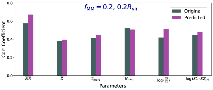
Figure 13: Comparison between the original correlation matrix and the predicted one using the Random Forest Regression for external drivers for the major merger mass-ratio above 0.2 and at $0.2R_{\mathrm{vir}}$ spatial cut. The fit corresponds to a $R^{2}=0.9$.

Appendix B Generalization to bigger sample: Random Forest Regression

In the main body of the paper, we analyzed the correlation coefficients between different internal and external parameters with $\Delta f^{j}_{\mathrm{eff}}$. While the level of correlation is significant for the parameter sets used, it is important to exercise caution regarding the generalizability of this analysis, given that our galaxy sample only includes 25 members.

To address the generalizability of the correlation coefficients between the external drivers and $\Delta f^{02}_{\mathrm{eff}}$, we employed Random Forest Regression to infer the predicted correlation coefficients between these quantities. Since the sample size is limited, instead of splitting the sample into training and test datasets, we utilized k-fold cross-validation. Our analysis indicated that using a k-fold value of 3 yielded a reasonable $R^{2}\simeq 0.34$, where $R^{2}$ represents the proportion of the variance in the dependent variable that is explained by the independent variables in the regression model. Consequently, we employed Random Forest Regression to infer the correlation coefficients.

Figure 13 compares the correlation coefficients from the original galaxy sample with those predicted by Random Forest Regression. The level of correlation is consistent between these methods. Furthermore, the model reported a reliable value for $R^{2}\simeq 0.9$, ensuring that these correlation coefficients can be representative of a larger system.

References

- Abadi et al. (2003) Abadi, M. G., Navarro, J. F., Steinmetz, M., & Eke, V. R. 2003, ApJ, 591, 499, doi: 10.1086/375512
- Bell et al. (2008) Bell, E. F., Zucker, D. B., Belokurov, V., et al. 2008, ApJ, 680, 295, doi: 10.1086/588032
- Belokurov et al. (2020) Belokurov, V., Sanders, J. L., Fattahi, A., et al. 2020, MNRAS, 494, 3880, doi: 10.1093/mnras/staa876
- Benson et al. (2004) Benson, A. J., Lacey, C. G., Frenk, C. S., Baugh, C. M., & Cole, S. 2004, MNRAS, 351, 1215, doi: 10.1111/j.1365-2966.2004.07870.x
- Bonaca et al. (2017) Bonaca, A., Conroy, C., Wetzel, A., Hopkins, P. F., & Kereš, D. 2017, ApJ, 845, 101, doi: 10.3847/1538-4357/aa7d0c
- Carollo & Chiba (2021) Carollo, D., & Chiba, M. 2021, ApJ, 908, 191, doi: 10.3847/1538-4357/abd7a4
- Conroy et al. (2019a) Conroy, C., Naidu, R. P., Zaritsky, D., et al. 2019a, ApJ, 887, 237, doi: 10.3847/1538-4357/ab5710
- Conroy et al. (2019b) Conroy, C., Bonaca, A., Cargile, P., et al. 2019b, ApJ, 883, 107, doi: 10.3847/1538-4357/ab38b8
- Cooper et al. (2015) Cooper, A. P., Parry, O. H., Lowing, B., Cole, S., & Frenk, C. 2015, MNRAS, 454, 3185, doi: 10.1093/mnras/stv2057
- Cui et al. (2012) Cui, X.-Q., Zhao, Y.-H., Chu, Y.-Q., et al. 2012, Research in Astronomy and Astrophysics, 12, 1197, doi: 10.1088/1674-4527/12/9/003
- de Buyl et al. (2016) de Buyl, P., Huang, M.-J., & Deprez, L. 2016, arXiv e-prints, arXiv:1608.04904. https://arxiv.org/abs/1608.04904
- De Lucia & Blaizot (2007) De Lucia, G., & Blaizot, J. 2007, MNRAS, 375, 2, doi: 10.1111/j.1365-2966.2006.11287.x
- De Silva et al. (2015) De Silva, G. M., Freeman, K. C., Bland-Hawthorn, J., et al. 2015, MNRAS, 449, 2604, doi: 10.1093/mnras/stv327
- Di Matteo et al. (2019) Di Matteo, P., Haywood, M., Lehnert, M. D., et al. 2019, A&A, 632, A4, doi: 10.1051/0004-6361/201834929
- Di Matteo et al. (2020) Di Matteo, P., Spite, M., Haywood, M., et al. 2020, A&A, 636, A115, doi: 10.1051/0004-6361/201937016
- Eggen et al. (1962) Eggen, O. J., Lynden-Bell, D., & Sandage, A. R. 1962, ApJ, 136, 748, doi: 10.1086/147433
- El-Badry et al. (2018) El-Badry, K., Quataert, E., Wetzel, A., et al. 2018, MNRAS, 473, 1930, doi: 10.1093/mnras/stx2482
- Elias et al. (2018) Elias, L. M., Sales, L. V., Creasey, P., et al. 2018, MNRAS, 479, 4004, doi: 10.1093/mnras/sty1718
- Emami et al. (2020a) Emami, R., Genel, S., Hernquist, L., et al. 2020a, arXiv e-prints, arXiv:2009.09220. https://arxiv.org/abs/2009.09220
- Emami et al. (2020b) Emami, R., Hernquist, L., Alcock, C., et al. 2020b, arXiv e-prints, arXiv:2012.12284. https://arxiv.org/abs/2012.12284
- Emami et al. (2022) Emami, R., Hernquist, L., Vogelsberger, M., et al. 2022, ApJ, 937, 20, doi: 10.3847/1538-4357/ac86c7
- Fattahi et al. (2020) Fattahi, A., Deason, A. J., Frenk, C. S., et al. 2020, MNRAS, 497, 4459, doi: 10.1093/mnras/staa2221
- Font et al. (2011) Font, A. S., McCarthy, I. G., Crain, R. A., et al. 2011, MNRAS, 416, 2802, doi: 10.1111/j.1365-2966.2011.19227.x
- Gaia Collaboration et al. (2016) Gaia Collaboration, Prusti, T., de Bruijne, J. H. J., et al. 2016, A&A, 595, A1, doi: 10.1051/0004-6361/201629272
- Gao et al. (2010) Gao, L., Theuns, T., Frenk, C. S., et al. 2010, MNRAS, 403, 1283, doi: 10.1111/j.1365-2966.2009.16225.x
- Genel et al. (2014) Genel, S., Vogelsberger, M., Springel, V., et al. 2014, MNRAS, 445, 175, doi: 10.1093/mnras/stu1654
- Griffen et al. (2018) Griffen, B. F., Dooley, G. A., Ji, A. P., et al. 2018, MNRAS, 474, 443, doi: 10.1093/mnras/stx2749
- Han et al. (2022) Han, J. J., Conroy, C., Johnson, B. D., et al. 2022, arXiv e-prints, arXiv:2208.04327. https://arxiv.org/abs/2208.04327
- Haywood et al. (2018) Haywood, M., Di Matteo, P., Lehnert, M. D., et al. 2018, ApJ, 863, 113, doi: 10.3847/1538-4357/aad235
- Hunter (2007) Hunter, J. D. 2007, Computing in Science and Engineering, 9, 90, doi: 10.1109/MCSE.2007.55
- Ishigaki et al. (2021) Ishigaki, M. N., Hartwig, T., Tarumi, Y., et al. 2021, MNRAS, 506, 5410, doi: 10.1093/mnras/stab1982
- Jean-Baptiste et al. (2017) Jean-Baptiste, I., Di Matteo, P., Haywood, M., et al. 2017, A&A, 604, A106, doi: 10.1051/0004-6361/201629691
- Kisku et al. (2021) Kisku, S., Schiavon, R. P., Horta, D., et al. 2021, MNRAS, 504, 1657, doi: 10.1093/mnras/stab525
- Mackereth et al. (2019) Mackereth, J. T., Schiavon, R. P., Pfeffer, J., et al. 2019, MNRAS, 482, 3426, doi: 10.1093/mnras/sty2955
- Majewski et al. (2017) Majewski, S. R., Schiavon, R. P., Frinchaboy, P. M., et al. 2017, AJ, 154, 94, doi: 10.3847/1538-3881/aa784d
- Matsuno et al. (2019) Matsuno, T., Aoki, W., & Suda, T. 2019, ApJ, 874, L35, doi: 10.3847/2041-8213/ab0ec0
- Matteucci (2021) Matteucci, F. 2021, A&A Rev., 29, 5, doi: 10.1007/s00159-021-00133-8
- McCarthy et al. (2012) McCarthy, I. G., Font, A. S., Crain, R. A., et al. 2012, MNRAS, 420, 2245, doi: 10.1111/j.1365-2966.2011.20189.x
- Monachesi et al. (2016a) Monachesi, A., Bell, E. F., Radburn-Smith, D. J., et al. 2016a, MNRAS, 457, 1419, doi: 10.1093/mnras/stv2987
- Monachesi et al. (2016b) Monachesi, A., Gómez, F. A., Grand, R. J. J., et al. 2016b, MNRAS, 459, L46, doi: 10.1093/mnrasl/slw052
- Monachesi et al. (2019) —. 2019, MNRAS, 485, 2589, doi: 10.1093/mnras/stz538
- Naidu et al. (2020) Naidu, R. P., Conroy, C., Bonaca, A., et al. 2020, ApJ, 901, 48, doi: 10.3847/1538-4357/abaef4
- Nelson et al. (2019a) Nelson, D., Pillepich, A., Springel, V., et al. 2019a, MNRAS, 490, 3234, doi: 10.1093/mnras/stz2306
- Nelson et al. (2019b) Nelson, D., Springel, V., Pillepich, A., et al. 2019b, Computational Astrophysics and Cosmology, 6, 2, doi: 10.1186/s40668-019-0028-x
- Oliphant (2007) Oliphant, T. E. 2007, Computing in Science and Engineering, 9, 10, doi: 10.1109/MCSE.2007.58
- Pillepich et al. (2015) Pillepich, A., Madau, P., & Mayer, L. 2015, ApJ, 799, 184, doi: 10.1088/0004-637X/799/2/184
- Pillepich et al. (2018) Pillepich, A., Springel, V., Nelson, D., et al. 2018, MNRAS, 473, 4077, doi: 10.1093/mnras/stx2656
- Pillepich et al. (2019) Pillepich, A., Nelson, D., Springel, V., et al. 2019, MNRAS, 490, 3196, doi: 10.1093/mnras/stz2338
- Planck Collaboration et al. (2016) Planck Collaboration, Ade, P. A. R., Aghanim, N., et al. 2016, A&A, 594, A13, doi: 10.1051/0004-6361/201525830
- Posti & Helmi (2019) Posti, L., & Helmi, A. 2019, A&A, 621, A56, doi: 10.1051/0004-6361/201833355
- Purcell et al. (2010) Purcell, C. W., Bullock, J. S., & Kazantzidis, S. 2010, MNRAS, 404, 1711, doi: 10.1111/j.1365-2966.2010.16429.x
- Qu et al. (2011) Qu, Y., Di Matteo, P., Lehnert, M. D., van Driel, W., & Jog, C. J. 2011, A&A, 535, A5, doi: 10.1051/0004-6361/201116502
- Rodriguez-Gomez et al. (2015) Rodriguez-Gomez, V., Genel, S., Vogelsberger, M., et al. 2015, MNRAS, 449, 49, doi: 10.1093/mnras/stv264
- Rodriguez-Gomez et al. (2016) Rodriguez-Gomez, V., Pillepich, A., Sales, L. V., et al. 2016, MNRAS, 458, 2371, doi: 10.1093/mnras/stw456
- Searle & Zinn (1978) Searle, L., & Zinn, R. 1978, ApJ, 225, 357, doi: 10.1086/156499
- Sestito et al. (2019) Sestito, F., Longeard, N., Martin, N. F., et al. 2019, MNRAS, 484, 2166, doi: 10.1093/mnras/stz043
- Sijacki et al. (2015) Sijacki, D., Vogelsberger, M., Genel, S., et al. 2015, MNRAS, 452, 575, doi: 10.1093/mnras/stv1340
- Steinmetz et al. (2006) Steinmetz, M., Zwitter, T., Siebert, A., et al. 2006, AJ, 132, 1645, doi: 10.1086/506564
- Tissera et al. (2014) Tissera, P. B., Beers, T. C., Carollo, D., & Scannapieco, C. 2014, MNRAS, 439, 3128, doi: 10.1093/mnras/stu181
- van der Walt et al. (2011) van der Walt, S., Colbert, S. C., & Varoquaux, G. 2011, Computing in Science and Engineering, 13, 22, doi: 10.1109/MCSE.2011.37
- Vogelsberger et al. (2014a) Vogelsberger, M., Genel, S., Springel, V., et al. 2014a, MNRAS, 444, 1518, doi: 10.1093/mnras/stu1536
- Vogelsberger et al. (2014b) —. 2014b, Nature, 509, 177, doi: 10.1038/nature13316
- Waskom et al. (2020) Waskom, M., Botvinnik, O., Ostblom, J., et al. 2020, mwaskom/seaborn: v0.10.0 (January 2020), v0.10.0, Zenodo, doi: 10.5281/zenodo.3629446
- Waters et al. (2024) Waters, T. K., Peterson, C., Emami, R., et al. 2024, ApJ, 961, 193, doi: 10.3847/1538-4357/ad165a
- Weinberger et al. (2017) Weinberger, R., Springel, V., Hernquist, L., et al. 2017, MNRAS, 465, 3291, doi: 10.1093/mnras/stw2944
- Yanny et al. (2009) Yanny, B., Rockosi, C., Newberg, H. J., et al. 2009, AJ, 137, 4377, doi: 10.1088/0004-6256/137/5/4377
- Zolotov et al. (2009) Zolotov, A., Willman, B., Brooks, A. M., et al. 2009, ApJ, 702, 1058, doi: 10.1088/0004-637X/702/2/1058
- Zolotov et al. (2010) —. 2010, ApJ, 721, 738, doi: 10.1088/0004-637X/721/1/738