Statistical mechanics of transfer learning in fully-connected networks in the proportional limit

Alessandro Ingrosso ingrosso@ictp.it The Abdus Salam International Centre for Theoretical Physics (ICTP), Trieste, Italy Rosalba Pacelli I.N.F.N., sezione di Padova, Via Marzolo 8, 35131, Padova, Italy Pietro Rotondo Dipartimento di Scienze Matematiche, Fisiche e Informatiche, Universitร  degli Studi di Parma, Parco Area delle Scienze, 7/A 43124 Parma, Italy Federica Gerace federica.gerace@unibo.it Dipartimento di Matematica, Universitร  di Bologna, Piazza di Porta San Donato 5, 40126, Bologna (BO), Italy
Abstract

Transfer learning (TL) is a well-established machine learning technique to boost the generalization performance on a specific (target) task using information gained from a related (source) task, and it crucially depends on the ability of a network to learn useful features. Leveraging recent analytical progress in the proportional regime of deep learning theory (i.e. the limit where the size of the training set $P$ and the size of the hidden layers $N$ are taken to infinity keeping their ratioย ฮฑ=P/N๐›ผ๐‘ƒ๐‘\alpha=P/N finite), in this work we develop a novel single-instance Franz-Parisi formalism that yields an effective theory for TL in fully-connected neural networks. Unlike the (lazy-training) infinite-width limit, where TL is ineffective, we demonstrate that in the proportional limit TL occurs due to a renormalized source-target kernel that quantifies their relatedness and determines whether TL is beneficial for generalization.

1 Introduction

Modern deep learning relies on foundation models that are pre-trained on tasks closely related to the one of interest but much richer in training examples. In this way, the generalization performance of a neural network trained on a data-scarce target task can consistently improve by leveraging the knowledge that the pre-trained model has previously acquired on a close but data-abundant source task. This Transfer Learning (TL) practice has amply demonstrated to enhance the generalization performance of deep learning models, especially in those settings where data is scarce or labelling is demandingย [1, 2].

Despite being among the dominating paradigms in deep learning applications, TL remains poorly understood from a theoretical perspective, with several fundamental questions still open. For instance, (i) how does the source-target similarity affect TL efficiency? (ii) how does the width of the transferred layers impact generalization performance?

Most theoretical results in this direction hold for a parallel form of TL in the framework of classical learning theory, and rely on proofs of worst-case bounds, based on the Vapnik-Chervonenkis dimensionย [3], covering number, stability, and Rademacher complexityย [4] (seeย [5, 6, 7] for review). A recent line of research has approached TL using statistical mechanicsย [8, 9, 10]. However its applicability is limited, since its focus is on linear NNs and source-target data models are overly simplistic. Inย [11], the authors went one step further by proposing a theoretical framework to study TL in one-hidden layer (1HL) and non-linear networks. Here, pre-training is purely numerical, the interaction between the source and target is encoded implicitly in the empirical covariance of the hidden units, and the first layer weights are always kept fixed to the source configurations.

The analytically tractable lazy-training infinite-width limitย [12, 13, 14, 15, 16], one of the recent milestones in deep learning theory, is also not a viable option to theoretically investigate pre-training and transfer stages: since the statistics of the weights remains unchanged during training, no features can be transferred from the source to the target taskย [17]. One possibility to overcome this issue is to consider the feature-learning phase of infinite-width networksย [18, 19, 20, 21, 22, 23, 24], where TL is still possibleย [25]. To investigate more realistic settings than the infinite-width limit, one could analyze TL in the recently-explored proportional regime of deep NNs, formally defined as the limit where both the size of the training set $P$ and the width of the hidden layers $N_{\ell}$ ($\ell=1,\dots,L$, $L$ being the depth of the network) scale to infinity while keeping the ratios $\alpha_{\ell}=P/N_{\ell}$ fixed. This limit has been firstly studied in linear networksย [26, 27, 28, 29] and then extended to non-linear modelsย [30, 31, 32]. One major advantage of such a setting is the possibility of corroborating its analytical predictions with the outcome of Bayesian learning experiments in finite-width networks, as recently done for fully-connected 1HL modelsย [33].

Refer to caption
Figure 1: Transfer learning in one-hidden layer networks through the lens of a single-instance Franz-Parisi framework. (a) Sketch of transfer learning with 1HL networks. The first-layers weights of the source (left) and target (right) networks are coupled, while the readout layers are optimized independently. The coupling strength is modulated by the parameter $\gamma$ (wavy yellow lines). The vertical displacement between the source and target networks represents the temporal displacement in their training, physically implemented by quenched averaging of the free-energy (equation above). (b) Learning curves of target 1HL networks. Experimental test loss (top) and squared norm of last layer weights (bottom) are shown as a function of source/target interaction strength $\gamma$ for different sizes $N_{1}$ and magnitudes of Gaussian prior $\lambda_{t,2}$ of the last layer. Markers are shown in comparison to solid lines, which represent theoretical predictions from the theory. The networks are trained on Ps=800subscript๐‘ƒ๐‘ 800P_{s}=800, $P_{t}=100$ examples from C-EMNIST (left) and C-CIFAR (right) tasks (see Appendix for more details on the tasks). Bars represent one standard deviation. The curves at $N_{1}=1000$ were obtained with source networks pre-trained on $784$-dimensional examples. The curves with $N_{1}=500$ refer to data projected in $D=300$ dimensions.

In this manuscript, we leverage the results established in the proportional limit, combining this approach with a novel single-instance Franz-Parisi formalismย [34] to investigate TL effectiveness in Bayesian NNs. In particular, we argue that the posterior over the weights of the source task plays the role of the quenched disorder in spin-glass theoryย [35], which can be thus integrated out using the well-known replica method. This leads to an explicit formula for the free-energy in the proportional limit, describing the learning scenario of a neural network trained on the target task while coupled to a quenched copy, pre-trained on the source task.

2 Single-instance Franz-Parisi formalism for Transfer Learning

In the standard TL pipeline, a neural network is trained on a $P_{t}$-dimensional target set $\mathcal{T}=(X_{t},y_{t})$ while keeping some of its layers frozen to the ones transferred from the Pssubscript๐‘ƒ๐‘ P_{s}-dimensional source set ๐’ฎ=(Xs,ys)๐’ฎsubscript๐‘‹๐‘ subscript๐‘ฆ๐‘ \mathcal{S}=(X_{s},y_{s}). Deep learning practitioners can later add a fine-tuning stage, where the transferred layers are unfrozen and the whole network is trained on the target set using a smaller learning rate.

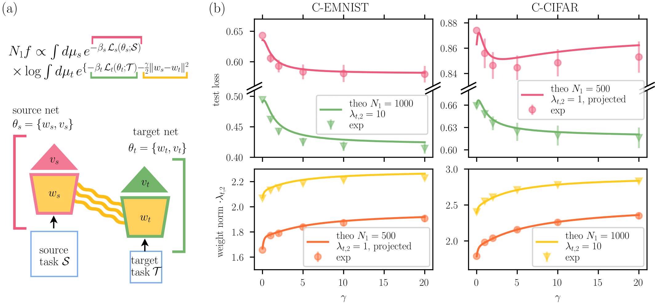
To rationalize the effectiveness of TL in the proportional limit of fully-connected networks, we introduce a novel approach based on statistical mechanics of learning [36]. Specifically, we consider a setting involving a one-hidden layer neural network $\phi_{t}$ whose first-layer weights adapt to the target task while coupled to those learned by another network ฯ•ssubscriptitalic-ฯ•๐‘ \phi_{s} on the source task. A sketch of the learning setting is shown in Fig.ย 1a. In the framework of statistical mechanics, this learning paradigm can be effectively described by the following free-energy density:

f=1N1โ€‹๐”ผฮธsโ€‹[logโ€‹โˆซ๐‘‘ฮผโ€‹(ฮธt)โ€‹eโˆ’ฮฒtโ€‹โ„’tโ€‹(ฮธt;๐’ฏ)โˆ’ฮณ2โ€‹โ€–wsโˆ’wtโ€–2],๐‘“1subscript๐‘1subscript๐”ผsubscript๐œƒ๐‘ delimited-[]differential-d๐œ‡subscript๐œƒ๐‘กsuperscript๐‘’subscript๐›ฝ๐‘กsubscriptโ„’๐‘กsubscript๐œƒ๐‘ก๐’ฏ๐›พ2superscriptnormsubscript๐‘ค๐‘ subscript๐‘ค๐‘ก2f=\frac{1}{N_{1}}\mathbb{E}_{\theta_{s}}\left[\log\int d\mu(\theta_{t})e^{-\beta_{t}\mathcal{L}_{t}\left(\theta_{t};\mathcal{T}\right)-\frac{\gamma}{2}\left\|w_{s}-w_{t}\right\|^{2}}\right], (1)

where $N_{1}$ is the number of hidden units, ฮธs/tsubscript๐œƒ๐‘ ๐‘ก\theta_{s/t} are the collections of the first and second-layer weights ws/tsubscript๐‘ค๐‘ ๐‘กw_{s/t} and vs/tsubscript๐‘ฃ๐‘ ๐‘กv_{s/t} of ฯ•s/tsubscriptitalic-ฯ•๐‘ ๐‘ก\phi_{s/t} respectively, $\mu(\theta_{t})$ is the Gaussian prior over the target weights, $\mathcal{L}_{t}$ is the target training loss, and $\beta_{t}$ is the target inverse temperature. The limit $\beta_{t}\to\infty$ can eventually enforce perfect interpolation of the target training set. The coupling between the source and the target network is controlled by a parameter $\gamma$. This allows for continuous interpolation between two regimes: one where the network is trained from scratch on the target set with no knowledge transfer from the source task ($\gamma=0$), and another one where the first-layer weights of the target network are kept frozen to the source weights, while the second-layer weights adapt to the target set ($\gamma\to\infty$). The intermediate values of $\gamma$ describe the fine-tuning stage, where the first-layer weights $w_{t}$ are first initialized to the source configuration wssubscript๐‘ค๐‘ w_{s} and then trained on the target set, together with the second-layer ones $v_{t}$. The expectation over the source configurations ฮธssubscript๐œƒ๐‘ \theta_{s} ensures we describe the typical TL behavior.

To guarantee that the source configurations effectively solve the source task, we take this expectation over the posterior distribution of the source weights. This corresponds to a Boltzmann-Gibbs measure whose partition function only involves the source task:

Zsโ€‹(ฮฒs)=โˆซ๐‘‘ฮผโ€‹(ฮธs)โ€‹eโˆ’ฮฒsโ€‹โ„’sโ€‹(ฮธs,๐’ฎ),subscript๐‘๐‘ subscript๐›ฝ๐‘ differential-d๐œ‡subscript๐œƒ๐‘ superscript๐‘’subscript๐›ฝ๐‘ subscriptโ„’๐‘ subscript๐œƒ๐‘ ๐’ฎZ_{s}\left(\beta_{s}\right)=\int d\mu\left(\theta_{s}\right)e^{-\beta_{s}\mathcal{L}_{s}\left(\theta_{s},\mathcal{S}\right)}, (2)

where ฮผโ€‹(ฮธs)๐œ‡subscript๐œƒ๐‘ \mu(\theta_{s}) is the Gaussian prior over the source weights and ฮฒssubscript๐›ฝ๐‘ \beta_{s} is the source inverse temperature. It is important to emphasize that, since the source and target training are not performed simultaneously, the expectation over the source configurations is quenched. This is crucial to ensure that the source posterior is not affected by the source-target coupling: in a TL pipeline, the source network is indeed trained on the source task without relying on any information on the target data.

As anticipated, the free-energy density in Eq.ย (1) closely resembles the Franz-Parisi potential, originally introduced to analyze metastable states in spin-glass systemsย [34] and later used to characterize the properties of energy landscapes in machine learning problemsย [37, 38] or knowledge distillationย [39] and curriculum learningย [40].

At variance with previous literatureย [41, 42], we refrain from averaging the free-energy density over the input data distribution, in the same spirit of Refs. ย [26, 30, 32, 31, 23] (note that a similar approach has been put forward to investigate Markov proximal learningย [43], in an attempt to connect the neural tangent and the neural network Gaussian process kernels).

For this reason, we name our new theoretical framework single instance Franz-Parisi. The quenched expectation over the source weights is tackled using the replica method, while the integral over the replicated target configurations in Eq.ย (1) is performed via the standard kernel renormalization approach, which is exact for deep linear networksย [26, 32], and can be justified using a Gaussian equivalence for non-linear activation function. In the following, we provide a sketch of the derivation [full details can be found in the Appendix], which is valid for quadratic loss function (mean squared error).

2.1 Free-energy in the proportional limit

To evaluate the quenched free-energy in Eq.ย (1) in the proportional thermodynamic limit described in the introduction, we make use of the replica trick:

f=1N1โ€‹1Zsโ€‹(ฮฒs)โ€‹limnโ†’0โˆ‚nZn.๐‘“1subscript๐‘11subscript๐‘๐‘ subscript๐›ฝ๐‘ subscriptโ†’๐‘›0subscript๐‘›superscript๐‘๐‘›f=\frac{1}{N_{1}}\frac{1}{Z_{s}\left(\beta_{s}\right)}\lim_{n\to 0}\partial_{n}Z^{n}. (3)

The calculation yields a compact expression for the replicated partition function in terms of an effective finite-$n$ action $S_{n}$, which, for the sake of simplicity and lighter notation, we here show in the case ฮฒt=ฮฒs=ฮฒsubscript๐›ฝ๐‘กsubscript๐›ฝ๐‘ ๐›ฝ\beta_{t}=\beta_{s}=\beta and ฮปs,2=ฮปt,2=ฮปsubscript๐œ†๐‘ 2subscript๐œ†๐‘ก2๐œ†\lambda_{s,2}=\lambda_{t,2}=\lambda:

$\displaystyle Z^{n}$ $\displaystyle\sim\mathrm{exp}\left\{N_{1}S_{n}(\mathcal{Q},\bar{\mathcal{Q}};n)\right\}$ (4)
$\displaystyle S_{n}$ $\displaystyle=\mathrm{Tr}\left(\lambda\mathcal{Q}\mathcal{\bar{Q}}\right)-\log\det\left(\mathbb{1}+\mathcal{\bar{Q}}\right)-\frac{1}{N_{1}}\log\det\left(\mathbb{1}+\beta\mathcal{K}\right)-\frac{\beta}{N_{1}}y^{T}\left(\mathbb{1}+\beta\mathcal{K}\right)^{-1}y$ (5)

where $\mathcal{Q}$ and its conjugate $\bar{\mathcal{Q}}$ are $(n+1)\times(n+1)$ order parameters matrices (see Appendix for the most general expression). At this level, $\mathcal{K}$ is a (Ps+nโ€‹Pt)ร—(Ps+nโ€‹Pt)subscript๐‘ƒ๐‘ ๐‘›subscript๐‘ƒ๐‘กsubscript๐‘ƒ๐‘ ๐‘›subscript๐‘ƒ๐‘ก\left(P_{s}+nP_{t}\right)\times\left(P_{s}+nP_{t}\right) replicated renormalized kernel matrix:

$\displaystyle\mathcal{K}_{\mu\nu}^{ab}=\mathcal{Q}^{ab}K^{ab}_{\mu\nu},\qquad\,\,K^{ab}_{\mu\nu}=\left\langle\sigma\left(h_{\mu}^{a}\right)\sigma\left(h_{\nu}^{b}\right)\right\rangle,$ (6)

where the expectations are taken over an effective distribution of the first-layer hidden representations $h$, and where the 00-th replica identifies the source network. Given the replica-symmetric nature of this problem, there are only four distinct order parameters ๐’ฌ={Qs,Qt,Qsโ€‹t,Qtโ€‹t}๐’ฌsubscript๐‘„๐‘ subscript๐‘„๐‘กsubscript๐‘„๐‘ ๐‘กsubscript๐‘„๐‘ก๐‘ก\mathcal{Q}=\{Q_{s},Q_{t},Q_{st},Q_{tt}\} โ€“ along with their conjugates $\bar{\mathcal{Q}}$ โ€“ mediating the interaction between the source and the target posterior distributions, via their coupling with four distinct kernels Kssubscript๐พ๐‘ K_{s}, $K_{t}$, Ksโ€‹tsubscript๐พ๐‘ ๐‘กK_{st}, $K_{tt}$. Of these, the crucial one is the effective source-target kernel Ksโ€‹tsubscript๐พ๐‘ ๐‘กK_{st}, computed on Gaussian pre-activations with covariance that depends on the overlap matrix between the inputs in the source and target task Csโ€‹t=Xsโ€‹XtT/N0subscript๐ถ๐‘ ๐‘กsubscript๐‘‹๐‘ superscriptsubscript๐‘‹๐‘ก๐‘‡subscript๐‘0C_{st}={X_{s}X_{t}^{T}}/{N_{0}}, with $N_{0}$ being the input dimension.

The $\mathcal{O}(1)$ terms of $S_{n}$ conspire to rebuild the effective action of the source task aloneย [30], while the $\mathcal{O}(n)$ terms in $S_{n}$ in the $n\to 0$ yield the genuine source-target action, incorporating the effect of transfer. Through appropriate derivatives of such transfer action, we can compute relevant observables in the equilibrium ensemble, e.g. the test loss or the statistics of the last-layer weights $\langle v^{2}\rangle$ (see Appendix).

Refer to caption
Figure 2: Effectiveness of fine-tuning is linked to correlation between source/target tasks. Top panel: test loss of 1HL target network is shown as a function of interaction strength with source network $\gamma$ for two values of correlation between source/target $\rho=0.1,0.5$. The source task comprises $P_{\textrm{source}}=800$ examples generated with a hidden manifold model with $N=500$ and latent dimension $D=300$. The $P_{\textrm{target}}=200$ target examples are build using a fraction $1-\rho$ of the source features, and a fraction $\rho$ of new ones. Middle and bottom panels: the order parameter $Q$ is shown as a function of $\gamma$ respectively for $\rho=0.1$ and $\rho=0.5$.

3 TL on benchmark tasks

Fig.ย 1b illustrates the good agreement between theoretical predictions (solid lines) and numerical simulations (dots) for both the test loss (first row) and the norm of the last-layer weights (second row), as a function of the coupling parameter $\gamma$, for two different values of $N_{1}$ and last-layer regularization strength $\lambda_{t,2}$. The two columns refer to TL scenarios with two different source-target pairs of binary tasks, namely C-EMNIST (left) and C-CIFAR (right), built from the well-known benchmark computer vision datasets EMNIST and CIFAR10. In particular, in the same spirit ofย [11], we build the source task by first dividing some classes of the original dataset into two groups, and then assigning one label per group. The target task is then obtained from the source task by changing one class per group. In this way, some of the features characterizing the source data are absent in the target set. This case is thus meant to describe settings where the source and target tasks are related but differ because of style or geometric structure of the input dataย [11].

The effectiveness of TL and fine-tuning strongly depends on data structure, and thus on the specific source-target relation, but also on the network size, as shown in Figย 1b. For instance, while there exists an optimal $\gamma$ minimizing the test loss in the C-CIFAR setup (right pink curve), the same does not occur with C-EMNIST (left pink curve), where the generalization performance steadily improves with $\gamma$, eventually reaching a plateau for $\gamma\to\infty$. At larger network sizes, the optimum in the C-CIFAR setup (left green curve) is attained at very large $\gamma$: fine-tuning is thus less beneficial than just freezing the features when converging towards the infinite-width limit. In the next two sections, we will focus on the impact of data structure and network width on TL.

3.1 Fine-Tuning and source-target similarity

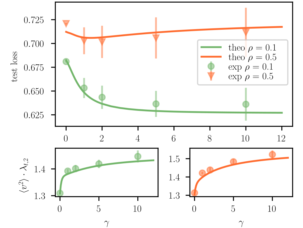
The level of source-target similarity is a crucial aspect in TL settings. If two tasks are poorly related, it is not unusual to observe negative transfer effectsย [44], up to the point where fixing the model parameters at random is more convenient than transferring those learned on the source taskย [11]. To analyze these aspects, we use the correlated hidden manifold (CHMM), a synthetic data model where source-target correlations are tuned via a set of parameters meant to mimic different and realistic TL scenarios. For instance, the source-target datasets may differ because of structure and style, as in the example in Fig.ย 1. In the model, this is described by the parameter $\rho$, which controls the fraction of source features that are replaced by new ones in the target set (more details on the CHMM can be found in Appendix).

Fig.ย 2 shows the test loss (top row) and norm of the weights (bottom row) as a function of $\gamma$, when training on a CHMM source-target pair with two distinct values of $\rho$. When a larger number of features are common to both tasks (green curve), the test loss decreases with the strength of the source-target coupling, showing that it is always convenient to constrain the first-layer weights to the source ones ($\gamma\to\infty$) rather than training from scratch ($\gamma$ = 0) or slightly fine-tuning the network on the target set (small $\gamma\to 0$). Instead, when the two tasks share only half of the features (orange curve), one clearly sees that freezing the first-layer weights does not lead to better generalization performance than training from scratch. In this case, a slight improvement is only attained by fine-tuning the network on the target set at $\gamma\simeq 1$.

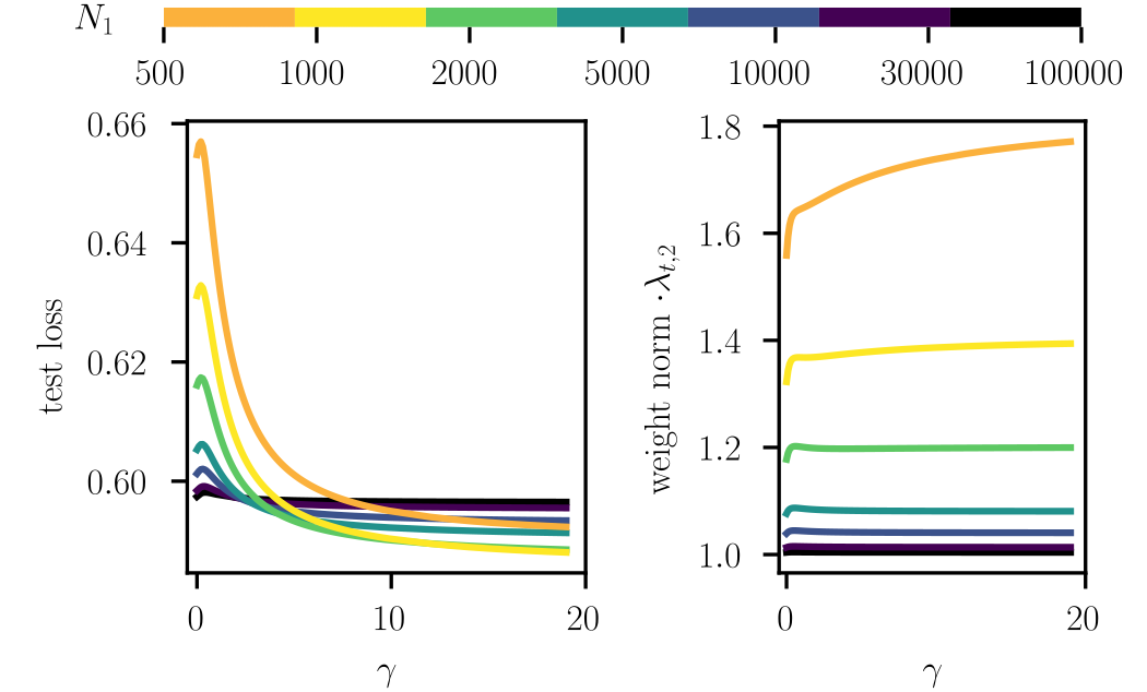
3.2 TL at proportional width VS infinite-width

Fig.ย 3 shows a comparison between the single-instance Franz-Parisi in the proportional regime and the infinite-width one. Specifically, we show test losses (left) and last-layer weight norms (right) of target networks for different values of $N_{1}$. Consistently, the theory reproduces the infinite-width limit behaviour in the regime where N1โ‰ซPs,Ptmuch-greater-thansubscript๐‘1subscript๐‘ƒ๐‘ subscript๐‘ƒ๐‘กN_{1}\gg P_{s},\,P_{t}. Already at N1โˆผ10โ€‹Pssimilar-tosubscript๐‘110subscript๐‘ƒ๐‘ N_{1}\sim 10P_{s}, there is less than $2\%$ gain in terms of generalization performance between uncoupled model to the best (completely transferred) model, and the last-layer weights have the same average norm as before the training ($1/\lambda_{t,2}$). This behavior is compatible with the lazy-training infinite-width regime, where the statistics of the weights of the source and target networks does not change during training, forbidding TL from being beneficial. More interestingly, already at $\gamma\sim 1$ smaller architectures do surpass the infinite-width performance, which is the best one for the uncoupled model. The fact that finite coupled networks outperform their best uncoupled predictor signals that the performance improvement is genuinely due to transfer and is not an artifact of effective regularization.

Refer to caption
Figure 3: Transfer learning is ineffective in the lazy-training infinite-width limit. Predicted test loss (left) and norm of last-layer weights (right) of the target network are shown as a function of the interaction strength $\gamma$ for different values of $N_{1}$. The task pair is C-EMNIST with Ps=800subscript๐‘ƒ๐‘ 800P_{s}=800, $P_{t}=100$. As the infinite-width limit is approached (N1โ‰ซPs,Ptmuch-greater-thansubscript๐‘1subscript๐‘ƒ๐‘ subscript๐‘ƒ๐‘กN_{1}\gg P_{s},P_{t} ), TL becomes ineffective, with no gain in terms of performance between the uncoupled model ($\gamma=0$) and the TL model ($\gamma>0$). Coherently, as $N_{1}$ grows, the last layer average weight norm converges to its prior value $1/\lambda_{t,1}$, corresponding to the infinite-width lazy-training solution $\mathcal{Q}=\mathbb{1}$ (Qs=Qt=1subscript๐‘„๐‘ subscript๐‘„๐‘ก1Q_{s}=Q_{t}=1, Qsโ€‹t=Qtโ€‹t=0subscript๐‘„๐‘ ๐‘กsubscript๐‘„๐‘ก๐‘ก0Q_{st}=Q_{tt}=0).

4 Discussion and Conclusions

In this work, we introduced a new theoretical approach to study TL in the proportional limit that leverages techniques used in the theory of spin glasses and kernel methods, and showcased it for 1HL fully connected networks. Our theory predicts the emergence of a source-target kernel Ksโ€‹tsubscript๐พ๐‘ ๐‘กK_{st}, whose renormalization in the proportional limit captures the improvement on generalization performance of the target network, when source and target tasks share some structure. More interestingly, the effect of transfer allows target networks to outperform the best predictor of the uncoupled models.

A transfer pipeline can also be formulated in convex problems where there is a strong imbalance between available data for two different learning tasks: linear regression tasks is arguably the simplest example of such a case where analytical expressions for TL can be derived without resorting to the replica method (see Appendix C and fig.ย 4 for a simple example in a teacher-student setting). The generalization to deep networks and more complex layer structures โ€“ where kernel renormalization has been shown to depend on a local mechanismย [31] โ€“ are interesting avenues for future work we are currently pursuing. In particular, we show in the Appendix how kernels would change for a convolutional layer, and sketch a tentative derivation for multi-layer architectures, which we conjecture to be exact in the case of deep linear networks.

Finally, it is reasonable to expect that the proposed effective theory breaks down in the large $P$ regimeย [45, 41, 46], i.e. when the number of training patterns is proportional to the total number of parameters of the network. Addressing this regime can be considered a major challenge for scientists working in deep learning theory.

Aknlowledgements

P.R. is supported by #NEXTGENERATIONEU (NGEU) and funded by the Ministry of University and Research (MUR), National Recovery and Resilience Plan (NRRP), project MNESYS (PE0000006) โ€œA Multiscale integrated approach to the study of the nervous system in health and diseaseโ€ (DN. 1553 11.10.2022). R.P. and P.R. thank Paolo Baglioni for fruitful discussions.

References

  • [1] Mรฉlanie Bernhardt, Danielย C Castro, Ryutaro Tanno, Anton Schwaighofer, Keremย C Tezcan, Miguel Monteiro, Shruthi Bannur, Matthewย P Lungren, Aditya Nori, Ben Glocker, etย al. Active label cleaning for improved dataset quality under resource constraints. Nature communications, 13(1):1161, 2022.
  • [2] Diana Mincu and Subhrajit Roy. Developing robust benchmarks for driving forward ai innovation in healthcare. Nature Machine Intelligence, 4(11):916โ€“921, 2022.
  • [3] Vladimir Vapnik. The nature of statistical learning theory. Springer science & business media, 2013.
  • [4] Peterย L Bartlett and Shahar Mendelson. Rademacher and gaussian complexities: Risk bounds and structural results. Journal of Machine Learning Research, 3(Nov):463โ€“482, 2002.
  • [5] Lei Zhang and Xinbo Gao. Transfer adaptation learning: A decade survey. IEEE Transactions on Neural Networks and Learning Systems, 2022.
  • [6] Yaqing Wang, Quanming Yao, Jamesย T Kwok, and Lionelย M Ni. Generalizing from a few examples: A survey on few-shot learning. ACM computing surveys (csur), 53(3):1โ€“34, 2020.
  • [7] Yuย Zhang and Qiang Yang. A survey on multi-task learning. IEEE Transactions on Knowledge and Data Engineering, 34(12):5586โ€“5609, 2021.
  • [8] Andrewย K Lampinen and Surya Ganguli. An analytic theory of generalization dynamics and transfer learning in deep linear networks. arXiv preprint arXiv:1809.10374, 2018.
  • [9] Yehuda Dar and Richardย G Baraniuk. Double double descent: on generalization errors in transfer learning between linear regression tasks. SIAM Journal on Mathematics of Data Science, 4(4):1447โ€“1472, 2022.
  • [10] Oussama Dhifallah and Yueย M Lu. Phase transitions in transfer learning for high-dimensional perceptrons. Entropy, 23(4):400, 2021.
  • [11] Federica Gerace, Luca Saglietti, Stefanoย Sarao Mannelli, Andrew Saxe, and Lenka Zdeborovรก. Probing transfer learning with a model of synthetic correlated datasets. Machine Learning: Science and Technology, 3(1):015030, 2022.
  • [12] Radfordย M. Neal. Priors for Infinite Networks, pages 29โ€“53. Springer New York, New York, NY, 1996.
  • [13] Jaehoon Lee, Jascha Sohl-dickstein, Jeffrey Pennington, Roman Novak, Sam Schoenholz, and Yasaman Bahri. Deep neural networks as gaussian processes. In International Conference on Learning Representations, 2018.
  • [14] Arthur Jacot, Franck Gabriel, and Clement Hongler. Neural tangent kernel: Convergence and generalization in neural networks. In S.ย Bengio, H.ย Wallach, H.ย Larochelle, K.ย Grauman, N.ย Cesa-Bianchi, and R.ย Garnett, editors, Advances in Neural Information Processing Systems, volumeย 31. Curran Associates, Inc., 2018.
  • [15] Alexanderย G. deย G.ย Matthews, Jiri Hron, Mark Rowland, Richardย E. Turner, and Zoubin Ghahramani. Gaussian process behaviour in wide deep neural networks. In International Conference on Learning Representations, 2018.
  • [16] Boris Hanin. Random neural networks in the infinite width limit as Gaussian processes. Ann. Appl. Probab., 33(6A):4798โ€“4819, 2023.
  • [17] Greg Yang and J.ย Edward Hu. Tensor programs iv: Feature learning in infinite-width neural networks. In International Conference on Machine Learning, 2021.
  • [18] Song Mei, Andrea Montanari, and Phan-Minh Nguyen. A mean field view of the landscape of two-layer neural networks. Proceedings of the National Academy of Sciences, 115(33):E7665โ€“E7671, 2018.
  • [19] Blake Bordelon and Cengiz Pehlevan. Self-consistent dynamical field theory of kernel evolution in wide neural networks. In S.ย Koyejo, S.ย Mohamed, A.ย Agarwal, D.ย Belgrave, K.ย Cho, and A.ย Oh, editors, Advances in Neural Information Processing Systems, volumeย 35, pages 32240โ€“32256. Curran Associates, Inc., 2022.
  • [20] Grant Rotskoff and Eric Vanden-Eijnden. Trainability and accuracy of artificial neural networks: An interacting particle system approach. Communications on Pure and Applied Mathematics, 75(9):1889โ€“1935, 2022.
  • [21] Justin Sirignano and Konstantinos Spiliopoulos. Mean field analysis of neural networks: A law of large numbers. SIAM Journal on Applied Mathematics, 80(2):725โ€“752, 2020.
  • [22] Lรฉnaรฏc Chizat and Francis Bach. On the global convergence of gradient descent for over-parameterized models using optimal transport. In S.ย Bengio, H.ย Wallach, H.ย Larochelle, K.ย Grauman, N.ย Cesa-Bianchi, and R.ย Garnett, editors, Advances in Neural Information Processing Systems, volumeย 31. Curran Associates, Inc., 2018.
  • [23] Inbar Seroussi, Gadi Naveh, and Zohar Ringel. Separation of scales and a thermodynamic description of feature learning in some cnns. Nature Communications, 14(1):908, 02 2023.
  • [24] Gadi Naveh and Zohar Ringel. A self consistent theory of gaussian processes captures feature learning effects in finite cnns. In M.ย Ranzato, A.ย Beygelzimer, Y.ย Dauphin, P.S. Liang, and J.ย Wortman Vaughan, editors, Advances in Neural Information Processing Systems, volumeย 34, pages 21352โ€“21364. Curran Associates, Inc., 2021.
  • [25] Greg Yang and Edwardย J Hu. Feature learning in infinite-width neural networks. arXiv preprint arXiv:2011.14522, 2020.
  • [26] Qianyi Li and Haim Sompolinsky. Statistical mechanics of deep linear neural networks: The backpropagating kernel renormalization. Phys. Rev. X, 11:031059, Sep 2021.
  • [27] Boris Hanin and Alexander Zlokapa. Bayesian interpolation with deep linear networks. Proceedings of the National Academy of Sciences, 120(23):e2301345120, 2023.
  • [28] Federico Bassetti, Marco Gherardi, Alessandro Ingrosso, Mauro Pastore, and Pietro Rotondo. Feature learning in finite-width bayesian deep linear networks with multiple outputs and convolutional layers. arXiv preprint arXiv:2406.03260, 2024.
  • [29] Lorenzo Tiberi, Francesca Mignacco, Kazuki Irie, and Haim Sompolinsky. Dissecting the interplay of attention paths in a statistical mechanics theory of transformers. arXiv preprint arXiv:2405.15926, 2024.
  • [30] Rย Pacelli, Sย Ariosto, Mย Pastore, Fย Ginelli, Mย Gherardi, and Pย Rotondo. A statistical mechanics framework for bayesian deep neural networks beyond the infinite-width limit. Nature Machine Intelligence, 5(12):1497โ€“1507, 2023.
  • [31] R.ย Aiudi, R.ย Pacelli, A.ย Vezzani, R.ย Burioni, and P.ย Rotondo. Local Kernel Renormalization as a mechanism for feature learning in overparametrized Convolutional Neural Networks. arXiv e-prints, page arXiv:2307.11807, July 2023.
  • [32] Qianyi Li and Haim Sompolinsky. Globally gated deep linear networks. Advances in Neural Information Processing Systems, 35:34789โ€“34801, 2022.
  • [33] P.ย Baglioni, R.ย Pacelli, R.ย Aiudi, F.ย Di Renzo, A.ย Vezzani, R.ย Burioni, and P.ย Rotondo. Predictive power of a bayesian effective action for fully-connected one hidden layer neural networks in the proportional limit, 2024.
  • [34] Silvio Franz and Giorgio Parisi. Recipes for metastable states in spin glasses. Journal de Physique I, 5(11):1401โ€“1415, 1995.
  • [35] Marc Mรฉzard, Giorgio Parisi, and Miguelย Angel Virasoro. Spin glass theory and beyond: An Introduction to the Replica Method and Its Applications, volumeย 9. World Scientific Publishing Company, 1987.
  • [36] Andreas Engel and Christian Vanย den Broeck. Statistical mechanics of learning. Cambridge University Press, 2001.
  • [37] Carlo Baldassi, Alessandro Ingrosso, Carlo Lucibello, Luca Saglietti, and Riccardo Zecchina. Subdominant dense clusters allow for simple learning and high computational performance in neural networks with discrete synapses. Physical review letters, 115(12):128101, 2015.
  • [38] Carlo Baldassi, Federica Gerace, Carlo Lucibello, Luca Saglietti, and Riccardo Zecchina. Learning may need only a few bits of synaptic precision. Physical Review E, 93(5):052313, 2016.
  • [39] Luca Saglietti and Lenka Zdeborovรก. Solvable model for inheriting the regularization through knowledge distillation. In Mathematical and Scientific Machine Learning, pages 809โ€“846. PMLR, 2022.
  • [40] Luca Saglietti, Stefano Mannelli, and Andrew Saxe. An analytical theory of curriculum learning in teacher-student networks. Advances in Neural Information Processing Systems, 35:21113โ€“21127, 2022.
  • [41] Hugo Cui, Florent Krzakala, and Lenka Zdeborova. Bayes-optimal learning of deep random networks of extensive-width. In Andreas Krause, Emma Brunskill, Kyunghyun Cho, Barbara Engelhardt, Sivan Sabato, and Jonathan Scarlett, editors, Proceedings of the 40th International Conference on Machine Learning, volume 202 of Proceedings of Machine Learning Research, pages 6468โ€“6521. PMLR, 23โ€“29 Jul 2023.
  • [42] Francesco Camilli, Daria Tieplova, and Jean Barbier. Fundamental limits of overparametrized shallow neural networks for supervised learning. arXiv preprint arXiv:2307.05635, 2023.
  • [43] Yehonatan Avidan, Qianyi Li, and Haim Sompolinsky. Connecting ntk and nngp: A unified theoretical framework for neural network learning dynamics in the kernel regime. arXiv preprint arXiv:2309.04522, 2023.
  • [44] Federica Gerace, Diego Doimo, Stefanoย Sarao Mannelli, Luca Saglietti, and Alessandro Laio. Optimal transfer protocol by incremental layer defrosting. arXiv preprint arXiv:2303.01429, 2023.
  • [45] Qianyi Li, Ben Sorscher, and Haim Sompolinsky. Representations and generalization in artificial and brain neural networks. Proceedings of the National Academy of Sciences, 121(27):e2311805121, 2024.
  • [46] Fabiรกn Aguirre-Lรณpez, Silvio Franz, and Mauro Pastore. Random features and polynomial rules, 2024.
  • [47] Christopher Williams. Computing with infinite networks. In M.C. Mozer, M.ย Jordan, and T.ย Petsche, editors, Advances in Neural Information Processing Systems, volumeย 9. MIT Press, 1996.

Appendix

Appendix A Setting and notation

The output of a one-hidden layer fully connected network given a data point $x\in R^{N_{0}}$ is:

$$\phi\left(x\right)=\frac{1}{\sqrt{N_{1}}}\sum_{k=1}^{N_{1}}v_{k}\sigma\left(\sum_{i=1}^{N_{0}}w_{ki}x_{i}\right)$$ (7)

with $\sigma$ a non-linear function. We will use erf as an example of a symmetric, saturating function: generalization to other nonlinearities is straightforward. Given a dataset of inputs and outputs $\mathcal{D}=\left\{X,y\right\}$, with $X$ the usual design matrix $X=\left(X\right)_{\mu i}$, the loss function reads:

$$\mathcal{L}\left(\theta,\mathcal{D}\right)=\frac{1}{2}\sum_{x,y\in\mathcal{D}}\left[y-\phi\left(\theta,x\right)\right]^{2}$$ (8)

where $\theta\equiv\left\{w,v\right\}$ is a shorthand for the collection of first and second layer weights.

We consider the learning problem of a one-hidden layer target network whose first-layer weights are coupled via a parameter $\gamma$ to those of a previously trained source network. Let us consider three datasets Xssubscript๐‘‹๐‘ X_{s}, $X_{t}$, $X_{\tau}$ of size Pssubscript๐‘ƒ๐‘ P_{s}, $P_{t}$, $P_{\tau}$, respectively the training set for the source and target task, and test set for the target task, with their respective outputs yssubscript๐‘ฆ๐‘ y_{s}, $y_{t}$, $y_{\tau}$.

Performing the quenched average over the source posterior weights of the log-partition function of the transfer weight, we get to the following expression:

N1โ€‹f=1Zsโ€‹โˆซ๐‘‘ฮผsโ€‹(ws)โ€‹eโˆ’ฮฒsโ€‹โ„’sโ€‹(ws)โ€‹logโ€‹โˆซ๐‘‘ฮผtโ€‹(wt)โ€‹eโˆ’ฮฒtโ€‹โ„’tโ€‹(wt)โˆ’ฮณ2โ€‹โ€–wsโˆ’wtโ€–2subscript๐‘1๐‘“1subscript๐‘๐‘ differential-dsubscript๐œ‡๐‘ subscript๐‘ค๐‘ superscript๐‘’subscript๐›ฝ๐‘ subscriptโ„’๐‘ subscript๐‘ค๐‘ differential-dsubscript๐œ‡๐‘กsubscript๐‘ค๐‘กsuperscript๐‘’subscript๐›ฝ๐‘กsubscriptโ„’๐‘กsubscript๐‘ค๐‘ก๐›พ2superscriptnormsubscript๐‘ค๐‘ subscript๐‘ค๐‘ก2N_{1}f=\frac{1}{Z_{s}}\int d\mu_{s}\left(w_{s}\right)e^{-\beta_{s}\mathcal{L}_{s}\left(w_{s}\right)}\log\int d\mu_{t}\left(w_{t}\right)e^{-\beta_{t}\mathcal{L}_{t}\left(w_{t}\right)-\frac{\gamma}{2}\left\|w_{s}-w_{t}\right\|^{2}} (9)

where

dโ€‹ฮผs/tโ€‹(w)=dโ€‹wโ€‹eโˆ’ฮปs/t,12โ€‹โ€–wโ€–2โˆ’ฮปs/t,22โ€‹โ€–vโ€–2๐‘‘subscript๐œ‡๐‘ ๐‘ก๐‘ค๐‘‘๐‘คsuperscript๐‘’subscript๐œ†๐‘ ๐‘ก12superscriptnorm๐‘ค2subscript๐œ†๐‘ ๐‘ก22superscriptnorm๐‘ฃ2d\mu_{s/t}\left(w\right)=dwe^{-\frac{\lambda_{s/t,1}}{2}\left\|w\right\|^{2}-\frac{\lambda_{s/t,2}}{2}\left\|v\right\|^{2}} (10)

and

Zsโ€‹(ฮฒs)=โˆซ๐‘‘ฮผsโ€‹(ws)โ€‹eโˆ’ฮฒsโ€‹โ„’sโ€‹(ws)subscript๐‘๐‘ subscript๐›ฝ๐‘ differential-dsubscript๐œ‡๐‘ subscript๐‘ค๐‘ superscript๐‘’subscript๐›ฝ๐‘ subscriptโ„’๐‘ subscript๐‘ค๐‘ Z_{s}\left(\beta_{s}\right)=\int d\mu_{s}\left(w_{s}\right)e^{-\beta_{s}\mathcal{L}_{s}\left(w_{s}\right)} (11)

is the source partition function. To deal with the $\log$, we make use of the replica trick:

$$\log Z=\lim_{n\to 0}\partial_{n}Z^{n}$$ (12)

and we write the transfer free-entropy in terms of replicated variables as

$\displaystyle N_{1}f$ =1Zsโ€‹(ฮฒs)โ€‹limnโ†’0โˆ‚nโˆซ๐‘‘ฮผsโ€‹(ws)โ€‹โˆa=1ndโ€‹ฮผtโ€‹(wta)โ€‹eโˆ’ฮฒsโ€‹โ„’sโ€‹(ws)absent1subscript๐‘๐‘ subscript๐›ฝ๐‘ subscriptโ†’๐‘›0subscript๐‘›differential-dsubscript๐œ‡๐‘ subscript๐‘ค๐‘ superscriptsubscriptproduct๐‘Ž1๐‘›๐‘‘subscript๐œ‡๐‘กsuperscriptsubscript๐‘ค๐‘ก๐‘Žsuperscript๐‘’subscript๐›ฝ๐‘ subscriptโ„’๐‘ subscript๐‘ค๐‘ \displaystyle=\frac{1}{Z_{s}\left(\beta_{s}\right)}\lim_{n\to 0}\partial_{n}\int d\mu_{s}\left(w_{s}\right)\prod_{a=1}^{n}d\mu_{t}\left(w_{t}^{a}\right)e^{-\beta_{s}\mathcal{L}_{s}\left(w_{s}\right)}
eโˆ’ฮฒtโ€‹โˆ‘a=1nโ„’tโ€‹({wta})โˆ’ฮณ2โ€‹โˆ‘aโ€–wsโˆ’wtaโ€–2.superscript๐‘’subscript๐›ฝ๐‘กsuperscriptsubscript๐‘Ž1๐‘›subscriptโ„’๐‘กsuperscriptsubscript๐‘ค๐‘ก๐‘Ž๐›พ2subscript๐‘Žsuperscriptnormsubscript๐‘ค๐‘ superscriptsubscript๐‘ค๐‘ก๐‘Ž2\displaystyle e^{-\beta_{t}\sum_{a=1}^{n}\mathcal{L}_{t}\left(\left\{w_{t}^{a}\right\}\right)-\frac{\gamma}{2}\sum_{a}\left\|w_{s}-w_{t}^{a}\right\|^{2}}\,. (13)

Eq. (13) represents a single-instance generalization of the classic disordered-averaged Franz-Parisi approach, originally developed to study metastable states in spin-glasses. We can employ $f$ to compute the posterior average of relevant quantities, such as training error, weight norms and distance across weight matrices, using simple differentiation:

$\displaystyle\mathcal{\epsilon}_{t}\equiv\left\langle\mathcal{L}_{t}\right\rangle=-\frac{N_{1}}{P_{t}}\partial_{\beta_{t}}f\,,$ (14)
$\displaystyle\left\|w_{t}\right\|^{2}=-2N_{1}\partial_{\lambda}f\,,$ (15)
โ€–wsโˆ’wtโ€–2=2โ€‹N1โ€‹โˆ‚ฮณf.superscriptnormsubscript๐‘ค๐‘ subscript๐‘ค๐‘ก22subscript๐‘1subscript๐›พ๐‘“\displaystyle\left\|w_{s}-w_{t}\right\|^{2}=2N_{1}\partial_{\gamma}f\,. (16)

The calculation of the generalization error is slightly more involved: we introduce and additional term $\beta_{\tau}\mathcal{L}_{\tau}\left(\left\{w_{t}\right\}\right)$ in the target Hamiltonian, where $\mathcal{L}_{\tau}\left(\left\{w_{t}\right\}\right)=\frac{1}{2}\sum_{\mu=1}^{P_{\tau}}\left[y_{\tau}^{\mu}-\phi\left(\theta_{t},x_{\tau}^{\mu}\right)\right]^{2}$ is the loss computed on a test set composed of $P_{\tau}$ patterns, and evaluate the test error with the expression $\mathcal{\epsilon}_{\tau}\equiv\left\langle\mathcal{L}_{\tau}\right\rangle=-\frac{N_{1}}{P_{\tau}}\partial_{\beta_{\tau}}f|_{\beta_{\tau}=0}$.

Generalization to a one-hidden layer convolutional neural network

The output of a one-hidden layer convolutional neural network (CNN) with filters of size $M$ and stride $S$ can be written as:

$$\phi^{CNN}\left(x;\left\{w,v\right\}\right)=\frac{1}{\sqrt{N_{c}}}\sum_{i=1}^{N_{0}/S}\sum_{c}^{N_{c}}v_{i}^{c}\sigma\left(\frac{1}{\sqrt{M}}\sum_{m}w_{cm}x_{Si+m}\right)\,.$$ (17)

Very few changes are in order to generalize our calculation to the case of a shallow CNN, which we will thus highlight along the way.

A.1 Notation

We use the 00 index for all weights and parameters involving the source, thus denoting the prior inverse variances in each layer $l$ as ฮปl0=ฮปs,lsuperscriptsubscript๐œ†๐‘™0subscript๐œ†๐‘ ๐‘™\lambda_{l}^{0}=\lambda_{s,l} and $\lambda_{l}^{a}\equiv\lambda_{t,l}$ for $a>0$. We thus treat $\left(a,\mu\right)$ as a multi-index over a construction with concatenated source and replicated target inputs [Xs,Xt,โ€ฆโ€‹XtโŸn]subscript๐‘‹๐‘ subscriptโŸsubscript๐‘‹๐‘กโ€ฆsubscript๐‘‹๐‘ก๐‘›[X_{s},\underbrace{X_{t},...X_{t}}_{n}], and trust the context to make the summation over $\mu$ clear. The same is done for the inverse temperatures, i.e. we have ฮฒฮผ0=ฮฒssuperscriptsubscript๐›ฝ๐œ‡0subscript๐›ฝ๐‘ \beta_{\mu}^{0}=\beta_{s} and $\beta_{\mu}^{a}=\beta_{t}$ for $a>0$. All sums over $a$ will implicitly run from 00 to $n$, unless specified by the subscript.

We will denote by $\mathbb{1}_{m}$ the identity matrix in dimension $m$, the vector $\left(e_{m}^{j}\right)_{i}=\delta_{ij}$ is the canonical base vector and $\left(\mathbb{I}_{m}\right)_{i}=1$ the constant vector of value $1$. We will usually drop the subscript when the dimension $m$ is implied by the context. We denote by $\mathcal{N}\left(h;m,C\right)$ a Gaussian distribution with mean $m$ and covariance $C$ over the vector $h$. All subleading factors will be discarded to reduce clutter.

Appendix B Transfer learning in a one-hidden layer networks

Our aim is to compute the following replicated partition function:

$\displaystyle Z^{n}=$ $\displaystyle\int\prod_{ki}dw_{ki}e^{-\frac{1}{2}\sum_{a}\lambda_{1}^{a}\left\|w^{a}\right\|^{2}-\frac{\gamma}{2}\sum_{a}\left\|w^{0}-w^{a}\right\|^{2}}$
$\displaystyle\int\prod_{ak}dv_{k}^{a}e^{-\frac{1}{2}\sum\lambda_{2}^{a}\left\|v^{a}\right\|^{2}-\frac{1}{2}\sum_{a\mu}\beta_{\mu}^{a}\left(\sum_{k}\frac{v_{k}^{a}}{\sqrt{N_{1}}}\sigma\left(\frac{1}{\sqrt{N_{0}}}\sum_{i}w_{ki}^{a}x_{\mu i}^{a}\right)-y_{\mu}^{a}\right)^{2}}\,.$ (18)

We expect that the final form will read

$$Z^{n}\sim\int\mathcal{DQ}\mathcal{D\bar{Q}}e^{\frac{N_{1}}{2}nS\left(\mathcal{Q},\bar{\mathcal{Q}}\right)}\,,$$ (19)

with $\mathcal{Q}$ and $\mathcal{\bar{Q}}$ a set of order parameters whose values will be determined by saddle-point equations. The $\mathcal{O}\left(1\right)$ component eN12โ€‹Ssโ€‹(Qs,Qยฏs)superscript๐‘’subscript๐‘12subscript๐‘†๐‘ subscript๐‘„๐‘ subscriptยฏ๐‘„๐‘ e^{\frac{N_{1}}{2}S_{s}\left(Q_{s},\bar{Q}_{s}\right)} of the replicated partition function $Z^{n}$ only depends on source order parameters and will cancel out with the term Zsโˆ’1superscriptsubscript๐‘๐‘ 1Z_{s}^{-1} at the saddle point.

B.1 Integrating first layer weights

Introducing the definition for the first-layer replicated pre-activations $h_{\mu k}^{a}=\frac{1}{\sqrt{N_{0}}}\sum_{i}w_{ki}^{a}x_{i}^{\mu a}$, we have:

$\displaystyle Z^{n}=$ $\displaystyle\int\prod_{ki}w_{ki}e^{-\frac{1}{2}\sum_{a}\lambda_{1}^{a}\left\|w\right\|^{2}-\frac{\gamma}{2}\sum_{a}\left\|w^{0}-w^{a}\right\|^{2}}$
$\displaystyle\int\prod_{\mu ak}d\bar{h}_{\mu k}^{a}dh_{\mu k}^{a}e^{i\sum_{a\mu k}\bar{h}_{\mu k}^{a}\left(\bar{h}_{k}^{a}-\frac{1}{\sqrt{N_{0}}}\sum_{i}w_{ki}^{a}x_{\mu i}^{a}\right)}$
$\displaystyle\int\prod_{ak}dv_{k}^{a}e^{-\frac{\lambda_{2}^{a}}{2}\sum_{a}\left\|v^{a}\right\|^{2}-\frac{1}{2}\sum_{a\mu}\beta_{\mu}^{a}\left(\sum_{k}\frac{v_{k}^{a}}{\sqrt{N_{1}}}\sigma\left(h_{\mu k}^{a}\right)-y_{\mu}^{a}\right)^{2}}\,.$ (20)

Let us isolate the dependence over the first layer pre-activations $h$ in the function $\psi$:

$\displaystyle\psi\left(h\right)$ $\displaystyle=\int\prod_{a\mu k}d\bar{h}_{\mu k}^{a}e^{i\sum_{a\mu k}\bar{h}_{\mu k}^{a}h_{\mu k}^{a}}$
$\displaystyle\int\mathcal{D}w\prod_{ki}e^{-\frac{1}{2}\sum_{ab}\Lambda_{1}^{ab}w_{ki}^{a}w_{ki}^{b}-\frac{i}{\sqrt{N_{0}}}\sum_{a\mu}w_{ki}^{a}\bar{h}_{\mu k}^{a}x_{\mu i}^{a}}$ (21)

where we have defined the following coupling matrix:

ฮ›1=(ฮปs,1โˆ’ฮณโˆ’ฮณโ€ฆโˆ’ฮณโˆ’ฮณฮปt,10โ€ฆ0โˆ’ฮณ0ฮปt,1โ€ฆโ€ฆโ€ฆโ€ฆโ€ฆโ€ฆ0โˆ’ฮณ0โ€ฆ0ฮปt,1)subscriptฮ›1subscript๐œ†๐‘ 1๐›พ๐›พโ€ฆ๐›พ๐›พsubscript๐œ†๐‘ก10โ€ฆ0๐›พ0subscript๐œ†๐‘ก1โ€ฆโ€ฆโ€ฆโ€ฆโ€ฆโ€ฆ0๐›พ0โ€ฆ0subscript๐œ†๐‘ก1\Lambda_{1}=\left(\begin{array}[]{ccccc}\lambda_{s,1}&-\gamma&-\gamma&...&-\gamma\\ -\gamma&\lambda_{t,1}&0&...&0\\ -\gamma&0&\lambda_{t,1}&...&...\\ ...&...&...&...&0\\ -\gamma&0&...&0&\lambda_{t,1}\end{array}\right) (22)

and $\mathcal{D}w\equiv\prod_{aki}dw_{ki}^{a}$. We thus write compactly:

$$Z^{n}=\int\mathcal{D}h\psi\left(h\right)\int\prod_{ak}dv_{l}^{a}e^{-\frac{1}{2}\sum_{a\mu}\beta_{\mu}^{a}\left(\sum_{k}\frac{v_{k}^{a}}{\sqrt{N_{1}}}\sigma\left(h_{\mu k}^{a}\right)-y_{\mu}^{a}\right)^{2}-\frac{\lambda_{2}^{a}}{2}\sum_{a}\left\|v^{a}\right\|^{2}}$$ (23)

and integrate over the weights

$$\psi\left(h\right)=\Delta_{1}\prod_{ki}\int\prod_{a\mu}d\bar{h}_{\mu k}^{a}e^{i\sum_{a\mu k}\bar{h}_{\mu k}^{a}\bar{h}_{\mu k}^{a}-\frac{1}{2}\sum_{ab}\Lambda_{ab}^{-1}\bar{q}_{ki}^{a}\left(\bar{h}\right)\bar{q}_{ki}^{b}\left(\bar{h}\right)}$$ (24)

with the definitions

$\displaystyle\bar{q}_{ki}^{a}\left(\bar{h}\right)=\frac{1}{\sqrt{N_{0}}}\sum_{\mu}\bar{h}_{\mu k}^{a}x_{\mu i}^{a}$ (25)
$\displaystyle\Delta_{1}=e^{-\frac{N_{1}N_{0}}{2}\log\det\Lambda}\,.$ (26)

We can write $Z^{n}$ in terms of the zero-mean, Gaussian distributed variables $h_{\mu k}^{a}$, whose covariance matrices $\tilde{C}$ read, for each $k$:

$$\tilde{C}_{\mu\nu}^{ab}=\left\langle h_{\mu k}^{a}h_{\mu k}^{b}\right\rangle=\Lambda_{ab}^{-1}C_{\mu\nu}^{ab}$$ (27)

where $C_{\mu\nu}^{ab}$ are replicated input covariances:

$$C_{\mu\nu}^{ab}=\frac{1}{N_{0}}\sum_{i=1}^{N_{0}}x_{\mu i}^{a}x_{\mu i}^{b}\,.$$ (28)

We thus have:

$$Z^{n}=\Delta_{1}\int\prod_{k}\mathcal{D}h_{k}\mathcal{D}v_{k}\mathcal{N}\left(h_{k};0,\tilde{C}\right)e^{-\frac{\lambda_{2}^{a}}{2}\sum_{a}\left\|v^{a}\right\|^{2}-\frac{1}{2}\sum_{a\mu}\beta_{\mu}^{a}\left(\sum_{k}\frac{v_{k}^{a}}{\sqrt{N_{1}}}\sigma\left(h_{\mu k}^{a}\right)-y_{\mu}^{a}\right)^{2}}$$ (29)

with $\mathcal{D}h_{k}\mathcal{D}v_{k}\equiv\prod_{a\mu}dh_{\mu k}^{a}\prod_{a}dv_{k}^{a}$.

Generalization to a 1-hl convolutional neural network

In the case of a convolutional layer, we would operate in the same manner and find $\bar{q}_{cm}^{a}=\frac{1}{\sqrt{M}}\sum_{\mu i}\bar{h}_{\mu ci}^{a}x_{Si+m}^{\mu}$. Note that variables $\bar{q}$ carry an additional index $c$ for each patch, so that $\mathcal{\bar{Q}}_{ab}$ is an $N_{c}\times N_{c}$ dimensional matrices, with $N_{c}$ the number of patches. The inter-patch input covariances reads:

$\displaystyle\tilde{C}_{\mu\nu}^{ab,ij}=\left\langle h_{\mu i}^{a}h_{\nu j}^{b}\right\rangle=\left(\Lambda^{-1}\right)^{ab}C_{\mu\nu}^{ab,ij}$ (30)
$\displaystyle C_{\mu\nu}^{ab,ij}=\frac{1}{M}\sum_{m}x_{Si+m}^{a,\mu}x_{Sj+m}^{b,\nu}\,.$ (31)

B.2 Integrating readout weights

Introducing the definition of the readout outputs sฮผa=โˆ‘kvkaN1โ€‹ฯƒโ€‹(hฮผโ€‹ka)superscriptsubscript๐‘ ๐œ‡๐‘Žsubscript๐‘˜superscriptsubscript๐‘ฃ๐‘˜๐‘Žsubscript๐‘1๐œŽsuperscriptsubscriptโ„Ž๐œ‡๐‘˜๐‘Žs_{\mu}^{a}=\sum_{k}\frac{v_{k}^{a}}{\sqrt{N_{1}}}\sigma\left(h_{\mu k}^{a}\right) with appropriate $\delta$ functions, we obtain an expression of the form

Zn=ฮ”1โ€‹โˆซ๐’Ÿโ€‹sโ€‹ฯˆโ€‹(s)superscript๐‘๐‘›subscriptฮ”1๐’Ÿ๐‘ ๐œ“๐‘ Z^{n}=\Delta_{1}\int\mathcal{D}s\psi\left(s\right) (32)

where

ฯˆโ€‹(s)=๐œ“๐‘ absent\displaystyle\psi\left(s\right)= โˆซ๐’Ÿโ€‹sโ€‹๐’Ÿโ€‹sยฏโ€‹โˆk๐’Ÿโ€‹hkโ€‹๐’Ÿโ€‹vkโ€‹๐’ฉโ€‹(hk;0,C~)๐’Ÿ๐‘ ๐’Ÿยฏ๐‘ subscriptproduct๐‘˜๐’Ÿsubscriptโ„Ž๐‘˜๐’Ÿsubscript๐‘ฃ๐‘˜๐’ฉsubscriptโ„Ž๐‘˜0~๐ถ\displaystyle\int\mathcal{D}s\mathcal{D}\bar{s}\prod_{k}\mathcal{D}h_{k}\mathcal{D}v_{k}\mathcal{N}\left(h_{k};0,\tilde{C}\right)
โˆkeโˆ’12โ€‹โˆ‘aฮป2aโ€‹(vka)2โ€‹eโˆ’iN1โ€‹โˆ‘aโ€‹ฮผsยฏฮผaโ€‹โˆ‘kvkaโ€‹ฯƒโ€‹(hฮผโ€‹ka)subscriptproduct๐‘˜superscript๐‘’12subscript๐‘Žsuperscriptsubscript๐œ†2๐‘Žsuperscriptsuperscriptsubscript๐‘ฃ๐‘˜๐‘Ž2superscript๐‘’๐‘–subscript๐‘1subscript๐‘Ž๐œ‡superscriptsubscriptยฏ๐‘ ๐œ‡๐‘Žsubscript๐‘˜superscriptsubscript๐‘ฃ๐‘˜๐‘Ž๐œŽsuperscriptsubscriptโ„Ž๐œ‡๐‘˜๐‘Ž\displaystyle\prod_{k}e^{-\frac{1}{2}\sum_{a}\lambda_{2}^{a}\left(v_{k}^{a}\right)^{2}}e^{-\frac{i}{\sqrt{N_{1}}}\sum_{a\mu}\bar{s}_{\mu}^{a}\sum_{k}v_{k}^{a}\sigma\left(h_{\mu k}^{a}\right)}
eiโ€‹โˆ‘aโ€‹ฮผsยฏฮผaโ€‹sฮผaโˆ’12โ€‹โˆ‘aโ€‹ฮผฮฒฮผaโ€‹(sฮผaโˆ’yฮผa)2superscript๐‘’๐‘–subscript๐‘Ž๐œ‡superscriptsubscriptยฏ๐‘ ๐œ‡๐‘Žsuperscriptsubscript๐‘ ๐œ‡๐‘Ž12subscript๐‘Ž๐œ‡superscriptsubscript๐›ฝ๐œ‡๐‘Žsuperscriptsuperscriptsubscript๐‘ ๐œ‡๐‘Žsuperscriptsubscript๐‘ฆ๐œ‡๐‘Ž2\displaystyle e^{i\sum_{a\mu}\bar{s}_{\mu}^{a}s_{\mu}^{a}-\frac{1}{2}\sum_{a\mu}\beta_{\mu}^{a}\left(s_{\mu}^{a}-y_{\mu}^{a}\right)^{2}} (33)

with the shorthand ๐’Ÿโ€‹sโ€‹๐’Ÿโ€‹sยฏ=โˆaโ€‹ฮผโ€‹kdโ€‹sฮผโ€‹kaโ€‹dโ€‹sยฏฮผโ€‹ka๐’Ÿ๐‘ ๐’Ÿยฏ๐‘ subscriptproduct๐‘Ž๐œ‡๐‘˜๐‘‘superscriptsubscript๐‘ ๐œ‡๐‘˜๐‘Ž๐‘‘superscriptsubscriptยฏ๐‘ ๐œ‡๐‘˜๐‘Ž\mathcal{D}s\mathcal{D}\bar{s}=\prod_{a\mu k}ds_{\mu k}^{a}d\bar{s}_{\mu k}^{a}. After a straghtforward integration over the uncoupled second-layer weights, we have:

ฯˆโ€‹(s)=๐œ“๐‘ absent\displaystyle\psi\left(s\right)= โˆซ๐’Ÿโ€‹sโ€‹๐’Ÿโ€‹sยฏโ€‹โˆk๐’Ÿโ€‹hkโ€‹๐’Ÿโ€‹vkโ€‹๐’ฉโ€‹(hk;0,C~)๐’Ÿ๐‘ ๐’Ÿยฏ๐‘ subscriptproduct๐‘˜๐’Ÿsubscriptโ„Ž๐‘˜๐’Ÿsubscript๐‘ฃ๐‘˜๐’ฉsubscriptโ„Ž๐‘˜0~๐ถ\displaystyle\int\mathcal{D}s\mathcal{D}\bar{s}\prod_{k}\mathcal{D}h_{k}\mathcal{D}v_{k}\mathcal{N}\left(h_{k};0,\tilde{C}\right)
ฮ”2โ€‹โˆkeโˆ’iN1โ€‹โˆ‘aโ€‹ฮผsยฏฮผaโ€‹sยฏฮฝaฮป2aโ€‹ฯƒโ€‹(hฮผโ€‹ka)โ€‹ฯƒโ€‹(hฮผโ€‹ka)subscriptฮ”2subscriptproduct๐‘˜superscript๐‘’๐‘–subscript๐‘1subscript๐‘Ž๐œ‡superscriptsubscriptยฏ๐‘ ๐œ‡๐‘Žsuperscriptsubscriptยฏ๐‘ ๐œˆ๐‘Žsuperscriptsubscript๐œ†2๐‘Ž๐œŽsuperscriptsubscriptโ„Ž๐œ‡๐‘˜๐‘Ž๐œŽsuperscriptsubscriptโ„Ž๐œ‡๐‘˜๐‘Ž\displaystyle\Delta_{2}\prod_{k}e^{-\frac{i}{N_{1}}\sum_{a\mu}\frac{\bar{s}_{\mu}^{a}\bar{s}_{\nu}^{a}}{\lambda_{2}^{a}}\sigma\left(h_{\mu k}^{a}\right)\sigma\left(h_{\mu k}^{a}\right)}
eiโ€‹โˆ‘aโ€‹ฮผsยฏฮผaโ€‹sฮผaโˆ’12โ€‹โˆ‘aโ€‹ฮผฮฒฮผaโ€‹(sฮผaโˆ’yฮผa)2superscript๐‘’๐‘–subscript๐‘Ž๐œ‡superscriptsubscriptยฏ๐‘ ๐œ‡๐‘Žsuperscriptsubscript๐‘ ๐œ‡๐‘Ž12subscript๐‘Ž๐œ‡superscriptsubscript๐›ฝ๐œ‡๐‘Žsuperscriptsuperscriptsubscript๐‘ ๐œ‡๐‘Žsuperscriptsubscript๐‘ฆ๐œ‡๐‘Ž2\displaystyle e^{i\sum_{a\mu}\bar{s}_{\mu}^{a}s_{\mu}^{a}-\frac{1}{2}\sum_{a\mu}\beta_{\mu}^{a}\left(s_{\mu}^{a}-y_{\mu}^{a}\right)^{2}} (34)

where we have introduced $\Delta_{2}=e^{-\frac{N_{1}}{2}\log\Lambda_{2}}$ using the second-layer coupling matrix

ฮ›2=(ฮปs,200โ€ฆ00ฮปt,20โ€ฆ000ฮปt,2โ€ฆโ€ฆโ€ฆโ€ฆโ€ฆโ€ฆ000โ€ฆ0ฮปt,2).subscriptฮ›2subscript๐œ†๐‘ 200โ€ฆ00subscript๐œ†๐‘ก20โ€ฆ000subscript๐œ†๐‘ก2โ€ฆโ€ฆโ€ฆโ€ฆโ€ฆโ€ฆ000โ€ฆ0subscript๐œ†๐‘ก2\Lambda_{2}=\left(\begin{array}[]{ccccc}\lambda_{s,2}&0&0&...&0\\ 0&\lambda_{t,2}&0&...&0\\ 0&0&\lambda_{t,2}&...&...\\ ...&...&...&...&0\\ 0&0&...&0&\lambda_{t,2}\end{array}\right)\,. (35)

We are now ready to employ the factorization over the first hidden layer index $k$ and consider the Gaussian variables $h_{\mu}^{a}$. Following the same strategy of Refs. [30, 31], we perform a self-consistent Gaussian approximation on the set of variables qยฏa=1ฮป2aโ€‹N1โ€‹โˆ‘ฮผsยฏฮผaโ€‹ฯƒโ€‹(hฮผa)superscriptยฏ๐‘ž๐‘Ž1superscriptsubscript๐œ†2๐‘Žsubscript๐‘1subscript๐œ‡superscriptsubscriptยฏ๐‘ ๐œ‡๐‘Ž๐œŽsuperscriptsubscriptโ„Ž๐œ‡๐‘Ž\bar{q}^{a}=\frac{1}{\sqrt{\lambda_{2}^{a}N_{1}}}\sum_{\mu}\bar{s}_{\mu}^{a}\sigma\left(h_{\mu}^{a}\right) in replica space, with order-parameter covariance matrix:

๐’ฌยฏaโ€‹b=โŸจqยฏaโ€‹qยฏbโŸฉ=1N1โ€‹ฮป2aโ€‹ฮป2bโ€‹โˆ‘ฮผโ€‹ฮฝsยฏฮผโ€‹ฮฝaโ€‹Kฮผโ€‹ฮฝaโ€‹bโ€‹sยฏฮผโ€‹ฮฝbsuperscriptยฏ๐’ฌ๐‘Ž๐‘delimited-โŸจโŸฉsuperscriptยฏ๐‘ž๐‘Žsuperscriptยฏ๐‘ž๐‘1subscript๐‘1superscriptsubscript๐œ†2๐‘Žsuperscriptsubscript๐œ†2๐‘subscript๐œ‡๐œˆsuperscriptsubscriptยฏ๐‘ ๐œ‡๐œˆ๐‘Žsuperscriptsubscript๐พ๐œ‡๐œˆ๐‘Ž๐‘superscriptsubscriptยฏ๐‘ ๐œ‡๐œˆ๐‘\mathcal{\bar{Q}}^{ab}=\left\langle\bar{q}^{a}\bar{q}^{b}\right\rangle=\frac{1}{N_{1}\sqrt{\lambda_{2}^{a}\lambda_{2}^{b}}}\sum_{\mu\nu}\bar{s}_{\mu\nu}^{a}K_{\mu\nu}^{ab}\bar{s}_{\mu\nu}^{b} (36)

and kernels:

$$K_{\mu\nu}^{ab}=\left\langle\sigma\left(h_{\mu}^{a}\right)\sigma\left(h_{\nu}^{a}\right)\right\rangle_{\mathcal{N}\left(h;0,\tilde{C}\right)}\,.$$ (37)

The relevant replicated kernels are:

K~s,ฮผโ€‹ฮฝ=subscript~๐พ๐‘ ๐œ‡๐œˆabsent\displaystyle\tilde{K}_{s,\mu\nu}= $\displaystyle\left\langle\sigma\left(h_{\mu}^{0}\right)\sigma\left(h_{\nu}^{0}\right)\right\rangle_{\mathcal{N}\left(h;0,\tilde{C}\right)}$ (38)
Ksโ€‹t,ฮผโ€‹ฮฝ=subscript๐พ๐‘ ๐‘ก๐œ‡๐œˆabsent\displaystyle K_{st,\mu\nu}= $\displaystyle\left\langle\sigma\left(h_{\mu}^{0}\right)\sigma\left(h_{\nu}^{a}\right)\right\rangle_{\mathcal{N}\left(h;0,\tilde{C}\right)}\qquad a>0$ (39)
$\displaystyle K_{t,\mu\nu}=$ $\displaystyle\left\langle\sigma\left(h_{\mu}^{a}\right)\sigma\left(h_{\nu}^{a}\right)\right\rangle_{\mathcal{N}\left(h;0,\tilde{C}\right)}\qquad a>0$ (40)
$\displaystyle K_{tt,\mu\nu}=$ โŸจฯƒโ€‹(hฮผa)โ€‹ฯƒโ€‹(hฮฝb)โŸฉ๐’ฉโ€‹(h;0,C~)aโ‰ b;a,b>0formulae-sequencesubscriptdelimited-โŸจโŸฉ๐œŽsuperscriptsubscriptโ„Ž๐œ‡๐‘Ž๐œŽsuperscriptsubscriptโ„Ž๐œˆ๐‘๐’ฉโ„Ž0~๐ถ๐‘Ž๐‘๐‘Ž๐‘0\displaystyle\left\langle\sigma\left(h_{\mu}^{a}\right)\sigma\left(h_{\nu}^{b}\right)\right\rangle_{\mathcal{N}\left(h;0,\tilde{C}\right)}\qquad a\neq b;a,b>0 (41)

with order parameters:

Qยฏs=๐’ฌยฏ00subscriptยฏ๐‘„๐‘ superscriptยฏ๐’ฌ00\displaystyle\bar{Q}_{s}=\bar{\mathcal{Q}}^{00} (42)
Qยฏsโ€‹t=๐’ฌยฏ0โ€‹aa>0formulae-sequencesubscriptยฏ๐‘„๐‘ ๐‘กsuperscriptยฏ๐’ฌ0๐‘Ž๐‘Ž0\displaystyle\bar{Q}_{st}=\mathcal{\bar{Q}}^{0a}\quad a>0 (43)
$\displaystyle\bar{Q}_{t}=\mathcal{\bar{Q}}^{aa}\quad\;a>0$ (44)
Qยฏtโ€‹t=๐’ฌยฏaโ€‹baโ‰ b;a,b>0.formulae-sequencesubscriptยฏ๐‘„๐‘ก๐‘กsuperscriptยฏ๐’ฌ๐‘Ž๐‘formulae-sequence๐‘Ž๐‘๐‘Ž๐‘0\displaystyle\bar{Q}_{tt}=\mathcal{\bar{Q}}^{ab}\quad a\neq b;\;a,b>0\,. (45)

Note that, at this stage, the kernels explicitly depend on the replica number $n$. Introducing the definitions of the order parameters with the help of appropriate $\delta$ functions and conjugate parameters $\mathcal{Q}$, we finally obtain:

$\displaystyle Z^{n}$ $\displaystyle=\Delta_{1}\Delta_{2}\int\mathcal{D}\mathcal{Q}\mathcal{D}\bar{\mathcal{Q}}e^{\frac{N_{1}}{2}\mathop{}\!\mathrm{Tr}\left(\tilde{\Lambda}_{2}\mathcal{Q}\mathcal{\bar{Q}}\right)-\frac{1}{2}\log\det\left(\mathbb{1}+\mathcal{\bar{Q}}\right)}$
โˆซ๐’Ÿโ€‹sโ€‹๐’Ÿโ€‹sยฏโ€‹eiโ€‹sยฏTโ€‹sโˆ’12โ€‹sยฏTโ€‹๐’ฆโ€‹sยฏโˆ’12โ€‹(sโˆ’y)Tโ€‹Bโ€‹(sโˆ’y)๐’Ÿ๐‘ ๐’Ÿยฏ๐‘ superscript๐‘’๐‘–superscriptยฏ๐‘ ๐‘‡๐‘ 12superscriptยฏ๐‘ ๐‘‡๐’ฆยฏ๐‘ 12superscript๐‘ ๐‘ฆ๐‘‡๐ต๐‘ ๐‘ฆ\displaystyle\int\mathcal{D}s\mathcal{D}\bar{s}e^{i\bar{s}^{T}s-\frac{1}{2}\bar{s}^{T}\mathcal{K}\bar{s}-\frac{1}{2}\left(s-y\right)^{T}B\left(s-y\right)} (46)

where $\mathcal{K}$ is the renormalized kernel $\mathcal{K}_{\mu\nu}^{ab}=\mathcal{Q}^{ab}K_{\mu\nu}^{ab}$ and $\left(\tilde{\Lambda}_{2}\right)_{ab}=\sqrt{\lambda_{2}^{a}\lambda_{2}^{b}}$. To simplify notation, we introduced a replicated vector (s)aโ€‹ฮผ=sฮผasubscript๐‘ ๐‘Ž๐œ‡superscriptsubscript๐‘ ๐œ‡๐‘Ž\left(s\right)_{a\mu}=s_{\mu}^{a} for the readout variables and targets $y_{\mu}^{a}$, and correspondingly for the diagonal matrix $B_{\mu\nu}^{ab}$ containing the inverse temperatures. More concretely, we have:

B=(ฮฒsโ€‹๐Ÿ™Ps00โ€ฆ00ฮฒtโ€‹๐Ÿ™Pt0โ€ฆ000ฮฒtโ€‹๐Ÿ™Ptโ€ฆโ€ฆโ€ฆโ€ฆโ€ฆโ€ฆ000ฮฒtโ€‹๐Ÿ™Pt)๐ตsubscript๐›ฝ๐‘ subscriptdouble-struck-๐Ÿ™subscript๐‘ƒ๐‘ 00โ€ฆ00subscript๐›ฝ๐‘กsubscriptdouble-struck-๐Ÿ™subscript๐‘ƒ๐‘ก0โ€ฆ000subscript๐›ฝ๐‘กsubscriptdouble-struck-๐Ÿ™subscript๐‘ƒ๐‘กmissing-subexpressionโ€ฆโ€ฆโ€ฆโ€ฆโ€ฆโ€ฆ000missing-subexpressionsubscript๐›ฝ๐‘กsubscriptdouble-struck-๐Ÿ™subscript๐‘ƒ๐‘กB=\left(\begin{array}[]{ccccc}\beta_{s}\mathbb{1}_{P_{s}}&0&0&...&0\\ 0&\beta_{t}\mathbb{1}_{P_{t}}&0&...&0\\ 0&0&\beta_{t}\mathbb{1}_{P_{t}}&&...\\ ...&...&...&...&...\\ 0&0&0&&\beta_{t}\mathbb{1}_{P_{t}}\end{array}\right) (47)

Integrating over sยฏยฏ๐‘ \bar{s} is straightforward:

$\displaystyle Z^{n}$ $\displaystyle=\Delta_{1}\Delta_{2}e^{-\frac{1}{2}y^{T}By}\int\mathcal{D}\mathcal{Q}\mathcal{D}\mathcal{\bar{Q}}e^{\frac{N_{1}}{2}\mathop{}\!\mathrm{Tr}\left(\tilde{\Lambda}_{2}\mathcal{Q}\mathcal{\bar{Q}}\right)-\frac{1}{2}\log\det\left(\mathbb{1}+\mathcal{\bar{Q}}\right)}$
eโˆ’12โ€‹sTโ€‹(B+๐’ฆโˆ’1)โ€‹s+sTโ€‹Bโ€‹yโˆ’12โ€‹logโ€‹det๐’ฆ.superscript๐‘’12superscript๐‘ ๐‘‡๐ตsuperscript๐’ฆ1๐‘ superscript๐‘ ๐‘‡๐ต๐‘ฆ12๐’ฆ\displaystyle e^{-\frac{1}{2}s^{T}\left(B+\mathcal{K}^{-1}\right)s+s^{T}By-\frac{1}{2}\log\det\mathcal{K}}\,. (48)

Further integrating over s๐‘ s, we find the final form valid for integer number replicas

$$Z^{n}=\int\mathcal{D}\mathcal{Q}\mathcal{D}\bar{\mathcal{Q}}e^{\frac{N_{1}}{2}S\left(\mathcal{Q},\mathcal{\bar{Q}}\right)}$$ (49)

where the finite-$n$ action is given by:

$\displaystyle S$ $\displaystyle=-N_{0}\log\det\Lambda_{1}-\log\det\Lambda_{2}+\mathop{}\!\mathrm{Tr}\left(\tilde{\Lambda}_{2}\mathcal{Q}\mathcal{\bar{Q}}\right)-\log\det\left(\mathbb{1}+\mathcal{\bar{Q}}\right)$
$\displaystyle-\frac{1}{N_{1}}\log\det{B\Sigma}-\frac{1}{N_{1}}y^{T}\Sigma^{-1}y,$ (50)

with

$$\Sigma=B^{-1}+\mathcal{K}$$ (51)
Generalization to a one-hidden layer convolutional neural network

In the case of a convolutional network, we would operate in the same manner and find $\bar{q}_{0,cm}^{CNN,a}=\frac{1}{\sqrt{M}}\sum_{\mu i}\bar{h}_{\mu ci}^{a}x_{Si+m}^{\mu}$, from which the replicated renormalized local kernel $\mathcal{K}_{\mu\nu}^{ab}=\sum_{ij}\mathcal{Q}_{ij}^{ab}K_{ij,\mu\nu}^{ab}$ is found.

B.3 Source and target action

As explained at the beginning of this section, the source-only action Sssubscript๐‘†๐‘ S_{s} can be easily obtained from the $\mathcal{O}\left(1\right)$ terms in $n$:

Sssubscript๐‘†๐‘ \displaystyle S_{s} =ฮปs,2โ€‹Qsโ€‹Qยฏsโˆ’logโก(1+Qยฏs)โˆ’1N1โ€‹logโ€‹detฮฒsโ€‹ฮฃsโˆ’1N1โ€‹ysโ€‹ฮฃsโˆ’1Tโ€‹ys+absentsubscript๐œ†๐‘ 2subscript๐‘„๐‘ subscriptยฏ๐‘„๐‘ 1subscriptยฏ๐‘„๐‘ 1subscript๐‘1subscript๐›ฝ๐‘ subscriptฮฃ๐‘ limit-from1subscript๐‘1subscript๐‘ฆ๐‘ superscriptsuperscriptsubscriptฮฃ๐‘ 1๐‘‡subscript๐‘ฆ๐‘ \displaystyle=\lambda_{s,2}Q_{s}\bar{Q}_{s}-\log\left(1+\bar{Q}_{s}\right)-\frac{1}{N_{1}}\log\det\beta_{s}\Sigma_{s}-\frac{1}{N_{1}}y_{s}{}^{T}\Sigma_{s}^{-1}y_{s}+
โˆ’N0โ€‹logโ€‹detฮปs,1โˆ’logโ€‹detฮปs,2subscript๐‘0subscript๐œ†๐‘ 1subscript๐œ†๐‘ 2\displaystyle-N_{0}\log\det\lambda_{s,1}-\log\det\lambda_{s,2} (52)

with

ฮฃs=๐Ÿ™ฮฒs+Qsโ€‹Kssubscriptฮฃ๐‘ double-struck-๐Ÿ™subscript๐›ฝ๐‘ subscript๐‘„๐‘ subscript๐พ๐‘ \Sigma_{s}=\frac{\mathbb{1}}{\beta_{s}}+Q_{s}K_{s} (53)

and Kssubscript๐พ๐‘ K_{s} the source-only first-layer kernel:

Ks,ฮผโ€‹ฮฝ=โŸจฯƒโ€‹(hฮผ)โ€‹ฯƒโ€‹(hฮฝ)โŸฉ๐’ฉโ€‹(h;0,Csฮปs,1)subscript๐พ๐‘ ๐œ‡๐œˆsubscriptdelimited-โŸจโŸฉ๐œŽsubscriptโ„Ž๐œ‡๐œŽsubscriptโ„Ž๐œˆ๐’ฉโ„Ž0subscript๐ถ๐‘ subscript๐œ†๐‘ 1K_{s,\mu\nu}=\left\langle\sigma\left(h_{\mu}\right)\sigma\left(h_{\nu}\right)\right\rangle_{\mathcal{N}\left(h;0,\frac{C_{s}}{\lambda_{s,1}}\right)} (54)

The values of Qssubscript๐‘„๐‘ Q_{s}, Qยฏssubscriptยฏ๐‘„๐‘ \bar{Q}_{s} are taken from the source-only saddle-point equations involved in determining Zssubscript๐‘๐‘ Z_{s}, as in the classic Franz-Parisi approach.

The genuine transfer action is obtained collecting the $\mathcal{O}\left(n\right)$ terms. The algebraic details involved in the diagonalization of the $\mathcal{Q}$ and $\Sigma$ matrices are collected in section B.6. Introducing the modified kernel matrices

$\displaystyle\Sigma_{t}=\frac{\mathcal{\mathbb{1}}}{\beta_{t}}+Q_{t}K_{t}$ (55)
$\displaystyle\Delta\Sigma_{t}=\Sigma_{t}-Q_{tt}K_{tt}$ (56)

and taking the $n\to 0$ limit, we finally have:

$$S=\Psi_{T}-\Psi_{\Delta}-\frac{1}{N_{1}}\Psi_{S}-\frac{1}{N_{1}}\Psi_{\mathcal{L}}$$ (57)

where

ฮจT=2โ€‹ฮปs,2โ€‹ฮปt,2โ€‹Qยฏsโ€‹tโ€‹Qsโ€‹t+ฮปt,2โ€‹(Qยฏtโ€‹Qtโˆ’Qยฏtโ€‹tโ€‹Qtโ€‹t)subscriptฮจ๐‘‡2subscript๐œ†๐‘ 2subscript๐œ†๐‘ก2subscriptยฏ๐‘„๐‘ ๐‘กsubscript๐‘„๐‘ ๐‘กsubscript๐œ†๐‘ก2subscriptยฏ๐‘„๐‘กsubscript๐‘„๐‘กsubscriptยฏ๐‘„๐‘ก๐‘กsubscript๐‘„๐‘ก๐‘ก\displaystyle\Psi_{T}=2\sqrt{\lambda_{s,2}\lambda_{t,2}}\bar{Q}_{st}Q_{st}+\lambda_{t,2}\left(\bar{Q}_{t}Q_{t}-\bar{Q}_{tt}Q_{tt}\right)
โˆ’logโก(1+Qยฏtโˆ’Qยฏtโ€‹t)โˆ’(1+Qยฏs)โ€‹Qยฏtโ€‹tโˆ’Qยฏsโ€‹t2(1+Qยฏs)โ€‹(1+Qยฏtโˆ’Qยฏtโ€‹t)1subscriptยฏ๐‘„๐‘กsubscriptยฏ๐‘„๐‘ก๐‘ก1subscriptยฏ๐‘„๐‘ subscriptยฏ๐‘„๐‘ก๐‘กsuperscriptsubscriptยฏ๐‘„๐‘ ๐‘ก21subscriptยฏ๐‘„๐‘ 1subscriptยฏ๐‘„๐‘กsubscriptยฏ๐‘„๐‘ก๐‘ก\displaystyle-\log\left(1+\bar{Q}_{t}-\bar{Q}_{tt}\right)-\frac{\left(1+\bar{Q}_{s}\right)\bar{Q}_{tt}-\bar{Q}_{st}^{2}}{\left(1+\bar{Q}_{s}\right)\left(1+\bar{Q}_{t}-\bar{Q}_{tt}\right)} (58)
ฮจฮ”=N0โ€‹(logโกฮป~+ฮปt,1โ€‹ฮณฮป~โ€‹ฮปs,1)+logโ€‹detฮปt,2subscriptฮจฮ”subscript๐‘0~๐œ†subscript๐œ†๐‘ก1๐›พ~๐œ†subscript๐œ†๐‘ 1subscript๐œ†๐‘ก2\displaystyle\Psi_{\Delta}=N_{0}\left(\log\tilde{\lambda}+\frac{\lambda_{t,1}\gamma}{\tilde{\lambda}\lambda_{s,1}}\right)+\log\det\lambda_{t,2} (59)
ฮจS=logโ€‹detฮฒtโ€‹ฮ”โ€‹ฮฃt+Qtโ€‹tโ€‹Trโ€‹(ฮ”โ€‹ฮฃtโˆ’1โ€‹Ktโ€‹t)โˆ’Qsโ€‹t2โ€‹Trโ€‹(ฮฃsโˆ’1โ€‹Ksโ€‹tโ€‹ฮ”โ€‹ฮฃtโˆ’1โ€‹Ksโ€‹tT)subscriptฮจ๐‘†subscript๐›ฝ๐‘กฮ”subscriptฮฃ๐‘กsubscript๐‘„๐‘ก๐‘กTrฮ”superscriptsubscriptฮฃ๐‘ก1subscript๐พ๐‘ก๐‘กsuperscriptsubscript๐‘„๐‘ ๐‘ก2Trsuperscriptsubscriptฮฃ๐‘ 1subscript๐พ๐‘ ๐‘กฮ”superscriptsubscriptฮฃ๐‘ก1superscriptsubscript๐พ๐‘ ๐‘ก๐‘‡\displaystyle\Psi_{S}=\log\det\beta_{t}\Delta\Sigma_{t}+Q_{tt}\mathop{}\!\mathrm{Tr}\left(\Delta\Sigma_{t}^{-1}K_{tt}\right)-Q_{st}^{2}\mathop{}\!\mathrm{Tr}\left(\Sigma_{s}^{-1}K_{st}\Delta\Sigma_{t}^{-1}K_{st}^{T}\right) (60)
ฮจโ„’=ytTโ€‹ฮ”โ€‹ฮฃtโˆ’1โ€‹ytTโˆ’2โ€‹Qsโ€‹tโ€‹ysTโ€‹ฮฃsโˆ’1โ€‹Ksโ€‹tโ€‹ฮ”โ€‹ฮฃtโˆ’1โ€‹yt+Qsโ€‹t2โ€‹ysTโ€‹ฮฃsโˆ’1โ€‹Ksโ€‹tโ€‹ฮ”โ€‹ฮฃtโˆ’1โ€‹Ksโ€‹tTโ€‹ฮฃsโˆ’1โ€‹yssubscriptฮจโ„’superscriptsubscript๐‘ฆ๐‘ก๐‘‡ฮ”superscriptsubscriptฮฃ๐‘ก1superscriptsubscript๐‘ฆ๐‘ก๐‘‡2subscript๐‘„๐‘ ๐‘กsuperscriptsubscript๐‘ฆ๐‘ ๐‘‡superscriptsubscriptฮฃ๐‘ 1subscript๐พ๐‘ ๐‘กฮ”superscriptsubscriptฮฃ๐‘ก1subscript๐‘ฆ๐‘กsuperscriptsubscript๐‘„๐‘ ๐‘ก2superscriptsubscript๐‘ฆ๐‘ ๐‘‡superscriptsubscriptฮฃ๐‘ 1subscript๐พ๐‘ ๐‘กฮ”superscriptsubscriptฮฃ๐‘ก1superscriptsubscript๐พ๐‘ ๐‘ก๐‘‡superscriptsubscriptฮฃ๐‘ 1subscript๐‘ฆ๐‘ \displaystyle\Psi_{\mathcal{L}}=y_{t}^{T}\Delta\Sigma_{t}^{-1}y_{t}^{T}-2Q_{st}y_{s}^{T}\Sigma_{s}^{-1}K_{st}\Delta\Sigma_{t}^{-1}y_{t}+Q_{st}^{2}y_{s}^{T}\Sigma_{s}^{-1}K_{st}\Delta\Sigma_{t}^{-1}K_{st}^{T}\Sigma_{s}^{-1}y_{s} (61)

with $\tilde{\lambda}=\lambda_{t,1}+\gamma$. The three relevant kernels for the target action are the following:

Ksโ€‹t,ฮผโ€‹ฮฝ=โŸจฯƒโ€‹(hฮผ)โ€‹ฯƒโ€‹(hฮฝ)โŸฉ๐’ฉโ€‹(h;0,C~sโ€‹t)subscript๐พ๐‘ ๐‘ก๐œ‡๐œˆsubscriptdelimited-โŸจโŸฉ๐œŽsubscriptโ„Ž๐œ‡๐œŽsubscriptโ„Ž๐œˆ๐’ฉโ„Ž0subscript~๐ถ๐‘ ๐‘ก\displaystyle K_{st,\mu\nu}=\left\langle\sigma\left(h_{\mu}\right)\sigma\left(h_{\nu}\right)\right\rangle_{\mathcal{N}\left(h;0,\tilde{C}_{st}\right)} (62)
$\displaystyle K_{t,\mu\nu}=\left\langle\sigma\left(h_{\mu}\right)\sigma\left(h_{\nu}\right)\right\rangle_{\mathcal{N}\left(h;0,\tilde{C}_{t}\right)}$ (63)
$\displaystyle K_{tt,\mu\nu}=\left\langle\sigma\left(h_{\mu}\right)\sigma\left(h_{\nu}\right)\right\rangle_{\mathcal{N}\left(h;0,\tilde{C}_{tt}\right)}$ (64)

where the source-target and target modified covariance matrices are given by

C~sโ€‹t=ฮณฮป~โ€‹ฮปs,1โ€‹Csโ€‹tsubscript~๐ถ๐‘ ๐‘ก๐›พ~๐œ†subscript๐œ†๐‘ 1subscript๐ถ๐‘ ๐‘ก\displaystyle\tilde{C}_{st}=\frac{\gamma}{\tilde{\lambda}\lambda_{s,1}}C_{st} (65)
C~t=1ฮป~โ€‹(1+ฮณ2ฮป~โ€‹ฮปs,1)โ€‹Ctsubscript~๐ถ๐‘ก1~๐œ†1superscript๐›พ2~๐œ†subscript๐œ†๐‘ 1subscript๐ถ๐‘ก\displaystyle\tilde{C}_{t}=\frac{1}{\tilde{\lambda}}\left(1+\frac{\gamma^{2}}{\tilde{\lambda}\lambda_{s,1}}\right)C_{t} (66)

and the inter-replica target kernel is computed using a matrix $\tilde{C}_{tt}$ with entries

C~tโ€‹t,ฮผโ€‹ฮฝ=ฮดฮผโ€‹ฮฝโ€‹C~t,ฮผโ€‹ฮผ+(1โˆ’ฮดฮผโ€‹ฮฝ)โ€‹ฮณ2ฮป~2โ€‹ฮปs,1โ€‹Ct,ฮผโ€‹ฮฝsubscript~๐ถ๐‘ก๐‘ก๐œ‡๐œˆsubscript๐›ฟ๐œ‡๐œˆsubscript~๐ถ๐‘ก๐œ‡๐œ‡1subscript๐›ฟ๐œ‡๐œˆsuperscript๐›พ2superscript~๐œ†2subscript๐œ†๐‘ 1subscript๐ถ๐‘ก๐œ‡๐œˆ\tilde{C}_{tt,\mu\nu}=\delta_{\mu\nu}\tilde{C}_{t,\mu\mu}+\left(1-\delta_{\mu\nu}\right)\frac{\gamma^{2}}{\tilde{\lambda}^{2}\lambda_{s,1}}C_{t,\mu\nu} (67)

where $\tilde{\lambda}\equiv\lambda_{t,1}+\gamma$. In the case of erf activation, we use the well known expression for the NNGP kernel [47]

$$\left\langle\sigma\left(h_{\mu}\right)\sigma\left(h_{\nu}\right)\right\rangle_{\mathcal{N}\left(h;0,C\right)}=\frac{2}{\pi}\arcsin\left(\frac{2C_{\mu\nu}}{\sqrt{\left(1+2C_{\mu\mu}\right)\left(1+2C_{\nu\nu}\right)}}\right).$$ (68)

B.4 SP equations

The SP equations for the order parameters read

ฮปs,2โ€‹ฮปt,2โ€‹Qsโ€‹t+Qยฏsโ€‹t(1+Qยฏs)โ€‹(1+Qยฏtโˆ’Qยฏtโ€‹t)=0subscript๐œ†๐‘ 2subscript๐œ†๐‘ก2subscript๐‘„๐‘ ๐‘กsubscriptยฏ๐‘„๐‘ ๐‘ก1subscriptยฏ๐‘„๐‘ 1subscriptยฏ๐‘„๐‘กsubscriptยฏ๐‘„๐‘ก๐‘ก0\displaystyle\sqrt{\lambda_{s,2}\lambda_{t,2}}Q_{st}+\frac{\bar{Q}_{st}}{\left(1+\bar{Q}_{s}\right)\left(1+\bar{Q}_{t}-\bar{Q}_{tt}\right)}=0 (69)
ฮปt,2โ€‹Qt=Qยฏsโ€‹t2+(1+Qยฏs)โ€‹(1+Qยฏtโˆ’2โ€‹Qยฏtโ€‹t)(1+Qยฏs)โ€‹(1+Qยฏtโˆ’Qยฏtโ€‹t)2subscript๐œ†๐‘ก2subscript๐‘„๐‘กsuperscriptsubscriptยฏ๐‘„๐‘ ๐‘ก21subscriptยฏ๐‘„๐‘ 1subscriptยฏ๐‘„๐‘ก2subscriptยฏ๐‘„๐‘ก๐‘ก1subscriptยฏ๐‘„๐‘ superscript1subscriptยฏ๐‘„๐‘กsubscriptยฏ๐‘„๐‘ก๐‘ก2\displaystyle\lambda_{t,2}Q_{t}=\frac{\bar{Q}_{st}^{2}+\left(1+\bar{Q}_{s}\right)\left(1+\bar{Q}_{t}-2\bar{Q}_{tt}\right)}{\left(1+\bar{Q}_{s}\right)\left(1+\bar{Q}_{t}-\bar{Q}_{tt}\right)^{2}} (70)
ฮปt,2โ€‹Qtโ€‹t=Qยฏsโ€‹t2โˆ’(1+Qยฏs)โ€‹Qยฏtโ€‹t(1+Qยฏs)โ€‹(1+Qยฏtโˆ’Qยฏtโ€‹t)2subscript๐œ†๐‘ก2subscript๐‘„๐‘ก๐‘กsuperscriptsubscriptยฏ๐‘„๐‘ ๐‘ก21subscriptยฏ๐‘„๐‘ subscriptยฏ๐‘„๐‘ก๐‘ก1subscriptยฏ๐‘„๐‘ superscript1subscriptยฏ๐‘„๐‘กsubscriptยฏ๐‘„๐‘ก๐‘ก2\displaystyle\lambda_{t,2}Q_{tt}=\frac{\bar{Q}_{st}^{2}-\left(1+\bar{Q}_{s}\right)\bar{Q}_{tt}}{\left(1+\bar{Q}_{s}\right)\left(1+\bar{Q}_{t}-\bar{Q}_{tt}\right)^{2}} (71)

whereas for the conjugate variables we have:

N1โ€‹ฮปs,2โ€‹ฮปt,2โ€‹Qยฏsโ€‹t=โˆ’Qsโ€‹tโ€‹Trโ€‹(ฮฃsโˆ’1โ€‹Ksโ€‹tโ€‹ฮ”โ€‹ฮฃtโˆ’1โ€‹Ksโ€‹tT)+Qsโ€‹tโ€‹ysTโ€‹ฮฃsโˆ’1โ€‹Ksโ€‹tโ€‹ฮ”โ€‹ฮฃtโˆ’1โ€‹Ksโ€‹tTโ€‹ฮฃsโˆ’1โ€‹yssubscript๐‘1subscript๐œ†๐‘ 2subscript๐œ†๐‘ก2subscriptยฏ๐‘„๐‘ ๐‘กsubscript๐‘„๐‘ ๐‘กTrsuperscriptsubscriptฮฃ๐‘ 1subscript๐พ๐‘ ๐‘กฮ”superscriptsubscriptฮฃ๐‘ก1superscriptsubscript๐พ๐‘ ๐‘ก๐‘‡subscript๐‘„๐‘ ๐‘กsuperscriptsubscript๐‘ฆ๐‘ ๐‘‡superscriptsubscriptฮฃ๐‘ 1subscript๐พ๐‘ ๐‘กฮ”superscriptsubscriptฮฃ๐‘ก1superscriptsubscript๐พ๐‘ ๐‘ก๐‘‡superscriptsubscriptฮฃ๐‘ 1subscript๐‘ฆ๐‘ \displaystyle N_{1}\sqrt{\lambda_{s,2}\lambda_{t,2}}\bar{Q}_{st}=-Q_{st}\mathop{}\!\mathrm{Tr}\left(\Sigma_{s}^{-1}K_{st}\Delta\Sigma_{t}^{-1}K_{st}^{T}\right)+Q_{st}y_{s}^{T}\Sigma_{s}^{-1}K_{st}\Delta\Sigma_{t}^{-1}K_{st}^{T}\Sigma_{s}^{-1}y_{s}
โˆ’Qsโ€‹tโ€‹ysTโ€‹ฮฃsโˆ’1โ€‹Ksโ€‹tโ€‹ฮ”โ€‹ฮฃtโˆ’1โ€‹ytsubscript๐‘„๐‘ ๐‘กsuperscriptsubscript๐‘ฆ๐‘ ๐‘‡superscriptsubscriptฮฃ๐‘ 1subscript๐พ๐‘ ๐‘กฮ”superscriptsubscriptฮฃ๐‘ก1subscript๐‘ฆ๐‘ก\displaystyle-Q_{st}y_{s}^{T}\Sigma_{s}^{-1}K_{st}\Delta\Sigma_{t}^{-1}y_{t} (72)
$\displaystyle N_{1}\lambda_{t,2}\bar{Q}_{t}=\mathop{}\!\mathrm{Tr}\left(\Delta\Sigma_{t}^{-1}K_{t}\right)-Q_{tt}\mathop{}\!\mathrm{Tr}\left(\Delta\Sigma_{t}^{-1}K_{t}\Delta\Sigma_{t}^{-1}K_{tt}\right)$
+Qsโ€‹t2โ€‹Trโ€‹(ฮฃsโˆ’1โ€‹Ksโ€‹tโ€‹ฮ”โ€‹ฮฃtโˆ’1โ€‹Ktโ€‹ฮ”โ€‹ฮฃtโˆ’1โ€‹Ksโ€‹tT)superscriptsubscript๐‘„๐‘ ๐‘ก2Trsuperscriptsubscriptฮฃ๐‘ 1subscript๐พ๐‘ ๐‘กฮ”superscriptsubscriptฮฃ๐‘ก1subscript๐พ๐‘กฮ”superscriptsubscriptฮฃ๐‘ก1superscriptsubscript๐พ๐‘ ๐‘ก๐‘‡\displaystyle+Q_{st}^{2}\mathop{}\!\mathrm{Tr}\left(\Sigma_{s}^{-1}K_{st}\Delta\Sigma_{t}^{-1}K_{t}\Delta\Sigma_{t}^{-1}K_{st}^{T}\right)
โˆ’Qsโ€‹t2โ€‹ysTโ€‹ฮฃsโˆ’1โ€‹Ksโ€‹tโ€‹ฮ”โ€‹ฮฃtโˆ’1โ€‹Ktโ€‹ฮ”โ€‹ฮฃtโˆ’1โ€‹Ksโ€‹tTโ€‹ฮฃsโˆ’1โ€‹ys+2โ€‹Qsโ€‹tโ€‹ysTโ€‹ฮฃsโˆ’1โ€‹Ksโ€‹tโ€‹ฮ”โ€‹ฮฃtโˆ’1โ€‹Ktโ€‹ฮ”โ€‹ฮฃtโˆ’1โ€‹ytsuperscriptsubscript๐‘„๐‘ ๐‘ก2superscriptsubscript๐‘ฆ๐‘ ๐‘‡superscriptsubscriptฮฃ๐‘ 1subscript๐พ๐‘ ๐‘กฮ”superscriptsubscriptฮฃ๐‘ก1subscript๐พ๐‘กฮ”superscriptsubscriptฮฃ๐‘ก1superscriptsubscript๐พ๐‘ ๐‘ก๐‘‡superscriptsubscriptฮฃ๐‘ 1subscript๐‘ฆ๐‘ 2subscript๐‘„๐‘ ๐‘กsuperscriptsubscript๐‘ฆ๐‘ ๐‘‡superscriptsubscriptฮฃ๐‘ 1subscript๐พ๐‘ ๐‘กฮ”superscriptsubscriptฮฃ๐‘ก1subscript๐พ๐‘กฮ”superscriptsubscriptฮฃ๐‘ก1subscript๐‘ฆ๐‘ก\displaystyle-Q_{st}^{2}y_{s}^{T}\Sigma_{s}^{-1}K_{st}\Delta\Sigma_{t}^{-1}K_{t}\Delta\Sigma_{t}^{-1}K_{st}^{T}\Sigma_{s}^{-1}y_{s}+2Q_{st}y_{s}^{T}\Sigma_{s}^{-1}K_{st}\Delta\Sigma_{t}^{-1}K_{t}\Delta\Sigma_{t}^{-1}y_{t}
$\displaystyle-y_{t}^{T}\Delta\Sigma_{t}^{-1}K_{t}\Delta\Sigma_{t}^{-1}y_{t}^{T}$ (73)
N1โ€‹ฮปt,2โ€‹Qยฏtโ€‹t=โˆ’Qtโ€‹tโ€‹Trโ€‹(ฮ”โ€‹ฮฃtโˆ’1โ€‹Ktโ€‹tโ€‹ฮ”โ€‹ฮฃtโˆ’1โ€‹Ktโ€‹t)+Qsโ€‹t2โ€‹Trโ€‹(ฮฃsโˆ’1โ€‹Ksโ€‹tโ€‹ฮ”โ€‹ฮฃtโˆ’1โ€‹Ktโ€‹tโ€‹ฮ”โ€‹ฮฃtโˆ’1โ€‹Ksโ€‹tT)+subscript๐‘1subscript๐œ†๐‘ก2subscriptยฏ๐‘„๐‘ก๐‘กsubscript๐‘„๐‘ก๐‘กTrฮ”superscriptsubscriptฮฃ๐‘ก1subscript๐พ๐‘ก๐‘กฮ”superscriptsubscriptฮฃ๐‘ก1subscript๐พ๐‘ก๐‘กlimit-fromsuperscriptsubscript๐‘„๐‘ ๐‘ก2Trsuperscriptsubscriptฮฃ๐‘ 1subscript๐พ๐‘ ๐‘กฮ”superscriptsubscriptฮฃ๐‘ก1subscript๐พ๐‘ก๐‘กฮ”superscriptsubscriptฮฃ๐‘ก1superscriptsubscript๐พ๐‘ ๐‘ก๐‘‡\displaystyle N_{1}\lambda_{t,2}\bar{Q}_{tt}=-Q_{tt}\mathop{}\!\mathrm{Tr}\left(\Delta\Sigma_{t}^{-1}K_{tt}\Delta\Sigma_{t}^{-1}K_{tt}\right)+Q_{st}^{2}\mathop{}\!\mathrm{Tr}\left(\Sigma_{s}^{-1}K_{st}\Delta\Sigma_{t}^{-1}K_{tt}\Delta\Sigma_{t}^{-1}K_{st}^{T}\right)+
โˆ’Qsโ€‹t2โ€‹ysTโ€‹ฮฃsโˆ’1โ€‹Ksโ€‹tโ€‹ฮ”โ€‹ฮฃtโˆ’1โ€‹Ktโ€‹tโ€‹ฮ”โ€‹ฮฃtโˆ’1โ€‹Ksโ€‹tTโ€‹ฮฃsโˆ’1โ€‹ys+2โ€‹Qsโ€‹tโ€‹ysTโ€‹ฮฃsโˆ’1โ€‹Ksโ€‹tโ€‹ฮ”โ€‹ฮฃtโˆ’1โ€‹Ktโ€‹tโ€‹ฮ”โ€‹ฮฃtโˆ’1โ€‹ytsuperscriptsubscript๐‘„๐‘ ๐‘ก2superscriptsubscript๐‘ฆ๐‘ ๐‘‡superscriptsubscriptฮฃ๐‘ 1subscript๐พ๐‘ ๐‘กฮ”superscriptsubscriptฮฃ๐‘ก1subscript๐พ๐‘ก๐‘กฮ”superscriptsubscriptฮฃ๐‘ก1superscriptsubscript๐พ๐‘ ๐‘ก๐‘‡superscriptsubscriptฮฃ๐‘ 1subscript๐‘ฆ๐‘ 2subscript๐‘„๐‘ ๐‘กsuperscriptsubscript๐‘ฆ๐‘ ๐‘‡superscriptsubscriptฮฃ๐‘ 1subscript๐พ๐‘ ๐‘กฮ”superscriptsubscriptฮฃ๐‘ก1subscript๐พ๐‘ก๐‘กฮ”superscriptsubscriptฮฃ๐‘ก1subscript๐‘ฆ๐‘ก\displaystyle-Q_{st}^{2}y_{s}^{T}\Sigma_{s}^{-1}K_{st}\Delta\Sigma_{t}^{-1}K_{tt}\Delta\Sigma_{t}^{-1}K_{st}^{T}\Sigma_{s}^{-1}y_{s}+2Q_{st}y_{s}^{T}\Sigma_{s}^{-1}K_{st}\Delta\Sigma_{t}^{-1}K_{tt}\Delta\Sigma_{t}^{-1}y_{t}
$\displaystyle-y_{t}^{T}\Delta\Sigma_{t}^{-1}K_{tt}\Delta\Sigma_{t}^{-1}y_{t}^{T}\,.$ (74)

B.5 Norm of the weights and generalization error

The norm of the second-layer weights can be easily obtained differentiating the action with respect to $\lambda_{t,2}$:

N1โ€‹โŸจโ€–vโ€–2โŸฉ=1ฮปt,2+Qtโ€‹tโ€‹Qยฏtโ€‹tโˆ’Qtโ€‹Qยฏtโˆ’ฮปs,2ฮปt,2โ€‹Qsโ€‹tโ€‹Qยฏsโ€‹tsubscript๐‘1delimited-โŸจโŸฉsuperscriptnorm๐‘ฃ21subscript๐œ†๐‘ก2subscript๐‘„๐‘ก๐‘กsubscriptยฏ๐‘„๐‘ก๐‘กsubscript๐‘„๐‘กsubscriptยฏ๐‘„๐‘กsubscript๐œ†๐‘ 2subscript๐œ†๐‘ก2subscript๐‘„๐‘ ๐‘กsubscriptยฏ๐‘„๐‘ ๐‘กN_{1}\left\langle\left\|v\right\|^{2}\right\rangle=\frac{1}{\lambda_{t,2}}+Q_{tt}\bar{Q}_{tt}-Q_{t}\bar{Q}_{t}-\sqrt{\frac{\lambda_{s,2}}{\lambda_{t,2}}}Q_{st}\bar{Q}_{st} (75)

As explained in section A, we can compute the generalization error by differentiating the free-energy with respect to an additional fictitious temperature $\beta_{\tau}$, coupled with a loss computed on a test set. This can be easily done by carrying out the previous calculation with an extended target dataset obtained by concatenating the input matrices $X_{\tilde{t}}=\left[X_{t},X_{\tau}\right]$ and output vectors $y_{\tilde{t}}=\left[y_{t},y_{\tau}\right]$. Accordingly, each target block in the matrix $B$ is extended so as to contain $P_{t}+P_{\tau}$ diagonal entries from the vector $\beta_{\mu}=(\underbrace{\beta_{t},...,\beta_{t}}_{P_{t}},\underbrace{\beta_{\tau},...,\beta_{\tau}}_{P_{\tau}})$. In what follows, the kernels Ksโ€‹t~subscript๐พ๐‘ ~๐‘กK_{s\tilde{t}}, $K_{\tilde{t}}$ and $K_{\tilde{t}\tilde{t}}$ are obtained from equations (62โ€“67) using covariance matrices from the extended dataset $X_{\tilde{t}}$. Calling $\Delta K=Q_{t}K_{\tilde{t}}-Q_{tt}K_{\tilde{t}\tilde{t}}$ and further denoting its test-test and train-test blocks respectively as $\Delta K_{\tau}$ and $\Delta K_{t\tau}$, we finally have for the generalization error:

$\displaystyle\epsilon_{\tau}$ $\displaystyle=\frac{1}{2}\mathop{}\!\mathrm{Tr}\left(\Delta K_{\tau}-\Delta K_{t\tau}^{T}\Delta\Sigma_{t}^{-1}\Delta K_{t\tau}\right)+\frac{1}{2}\left\|y_{\tau}-\Delta K_{t\tau}^{T}\Delta\Sigma_{t}^{-1}y_{t}\right\|^{2}+$
12โ€‹Qtโ€‹tโ€‹Trโ€‹(M~โ€‹Kt~โ€‹t~)โˆ’12โ€‹Qsโ€‹t2โ€‹Trโ€‹(ฮฃsโˆ’1โ€‹Ksโ€‹t~โ€‹M~โ€‹Ksโ€‹t~T)+12subscript๐‘„๐‘ก๐‘กTr~๐‘€subscript๐พ~๐‘ก~๐‘กlimit-from12superscriptsubscript๐‘„๐‘ ๐‘ก2Trsuperscriptsubscriptฮฃ๐‘ 1subscript๐พ๐‘ ~๐‘ก~๐‘€superscriptsubscript๐พ๐‘ ~๐‘ก๐‘‡\displaystyle\frac{1}{2}Q_{tt}\mathop{}\!\mathrm{Tr}\left(\tilde{M}K_{\tilde{t}\tilde{t}}\right)-\frac{1}{2}Q_{st}^{2}\mathop{}\!\mathrm{Tr}\left(\Sigma_{s}^{-1}K_{s\tilde{t}}\tilde{M}K_{s\tilde{t}}^{T}\right)+
12โ€‹Qsโ€‹t2โ€‹ysTโ€‹ฮฃsโˆ’1โ€‹Ksโ€‹t~โ€‹M~โ€‹Ksโ€‹t~Tโ€‹ฮฃsโˆ’1โ€‹ysโˆ’Qsโ€‹tโ€‹ysTโ€‹ฮฃsโˆ’1โ€‹Ksโ€‹t~โ€‹M~โ€‹yt~12superscriptsubscript๐‘„๐‘ ๐‘ก2superscriptsubscript๐‘ฆ๐‘ ๐‘‡superscriptsubscriptฮฃ๐‘ 1subscript๐พ๐‘ ~๐‘ก~๐‘€superscriptsubscript๐พ๐‘ ~๐‘ก๐‘‡superscriptsubscriptฮฃ๐‘ 1subscript๐‘ฆ๐‘ subscript๐‘„๐‘ ๐‘กsuperscriptsubscript๐‘ฆ๐‘ ๐‘‡superscriptsubscriptฮฃ๐‘ 1subscript๐พ๐‘ ~๐‘ก~๐‘€subscript๐‘ฆ~๐‘ก\displaystyle\frac{1}{2}Q_{st}^{2}y_{s}^{T}\Sigma_{s}^{-1}K_{s\tilde{t}}\tilde{M}K_{s\tilde{t}}^{T}\Sigma_{s}^{-1}y_{s}-Q_{st}y_{s}^{T}\Sigma_{s}^{-1}K_{s\tilde{t}}\tilde{M}y_{\tilde{t}} (76)

where the matrix $\tilde{M}$ reads:

$$\tilde{M}=\left(\begin{array}[]{cc}\Delta\Sigma_{t}^{-1}\Delta K_{t\tau}\Delta K_{t\tau}^{T}\Delta\Sigma_{t}^{-1}&-\Delta\Sigma_{t}^{-1}\Delta K_{t\tau}\\ -\Delta K_{t\tau}^{T}\Delta\Sigma_{t}^{-1}&\mathbb{1}_{P_{\tau}}\end{array}\right).$$ (77)

B.6 Some algebraic details in our derivation

Useful algebraic relations.

We gather here some algebraic relations involving a block-matrix $\mathcal{F}$, useful in both layer-wise integration of weights coupling and the ensuing calculations. Given four matrices $A,B,C,\Delta C$ with $A\in\mathbb{R}^{p_{1}\times p_{1}}$, $B\in\mathbb{R}^{p_{1}\times p_{2}}$ and $C,\Delta C\in\mathbb{R}^{p_{2}\times p_{2}}$, we call $\mathcal{F}$ the $\left(p_{1}+np_{2}\right)\times\left(p_{1}+np_{2}\right)$ dimensional block matrix of the form:

$$\mathcal{F}=\left(\begin{array}[]{cccc}A&B&B&B\\ B^{T}&C+\Delta C&C&C\\ B^{T}&C&C+\Delta C&C\\ B^{T}&C&C&C+\Delta C\end{array}\right)\,.$$ (78)

We can easily compute its inverse by first considering its lower-right $n\times n$ block

$$\mathcal{F}_{n}=\mathbb{1}_{n}\otimes\Delta C+\mathbb{I}_{n}\mathbb{I}_{n}^{T}\otimes C$$ (79)

where:

$\displaystyle\mathcal{F}_{n}^{-1}=\mathbb{1}_{n}\otimes\Delta C^{-1}+\mathbb{I}_{n}\mathbb{I}_{n}^{T}\otimes\bar{\mathcal{F}}$ (80)
$\displaystyle\bar{\mathcal{F}}=\frac{1}{n}\left[\left(\Delta C+nC\right)^{-1}-\Delta C^{-1}\right]=-\left(\Delta C+nC\right)^{-1}C\Delta C^{-1}\,.$ (81)

We have for $\mathcal{F}^{-1}$ the block structure:

$$\mathcal{F}^{-1}=\left(\begin{array}[]{cc}\mathcal{F}_{0}^{-1}&\mathbb{I}_{n}\otimes\mathcal{F}_{1}\\ \mathbb{I}_{n}^{T}\otimes\mathcal{F}_{1}^{T}&\mathcal{F}_{2,n}^{-1}\end{array}\right)$$ (82)

with the Schur complements and off-diagonal term reading:

$\displaystyle\mathcal{F}_{0}=A-nB\left(\Delta C+nC\right)^{-1}B^{T}$ (83)
$\displaystyle\mathcal{F}_{1}=-A^{-1}B\left(\Delta C+nC-nB^{T}A^{-1}B\right)^{-1}$ (84)
$\displaystyle\mathcal{F}_{2,n}=\mathbb{1}_{n}\otimes\Delta C+\mathbb{I}_{n}\mathbb{I}_{n}^{T}\otimes\left(C-B^{T}A^{-1}B\right)$ (85)
$\displaystyle\mathcal{F}_{2,n}^{-1}=\mathbb{1}_{n}\otimes\Delta C^{-1}+\mathbb{I}_{n}\mathbb{I}_{n}^{T}\otimes\frac{1}{n}\left[\left(\Delta C+n\bar{\mathcal{F}}_{2}\right)^{-1}-\Delta C^{-1}\right]$ (86)
$\displaystyle\bar{\mathcal{F}}_{2}=C-B^{T}A^{-1}B\,.$ (87)

As for the determinant of $\mathcal{F}$ one has:

$\displaystyle\log\det\mathcal{F}_{n}=\left(n-1\right)\log\det\Delta C+\mathop{}\!\mathrm{Tr}\log\left(\Delta C+nC\right)$ (88)
$\displaystyle\log\det\mathcal{F}=\log\det\mathcal{F}_{n}+\mathop{}\!\mathrm{Tr}\log\left(\mathcal{F}^{0}\right)\,.$ (89)

We will consider the contraction of $\mathcal{F}$ with a vector of the form $\tilde{y}=(y_{0},\underbrace{y,...,y}_{n})$:

$$\tilde{y}^{T}\mathcal{F}^{-1}\tilde{y}=y_{0}^{T}\mathcal{F}_{0}^{-1}y_{0}+2ny_{0}^{T}\mathcal{F}_{1}y+ny^{T}\left(\Delta C+n\bar{\mathcal{F}}_{2}\right)^{-1}y$$ (90)

Deriving the final action for transfer learning involves the $n\to 0$ limits of the previously computed quantities:

$\displaystyle\log\det\mathcal{F}_{n}\sim n\log\det\Delta C+n\mathop{}\!\mathrm{Tr}\left(\Delta C^{-1}C\right)$ (91)
$\displaystyle\mathop{}\!\mathrm{Tr}\log\mathcal{F}^{0}\sim\mathop{}\!\mathrm{Tr}\log A-n\mathop{}\!\mathrm{Tr}\left(A^{-1}B\Delta C^{-1}B^{T}\right)$ (92)
$\displaystyle\mathcal{F}_{0}^{-1}\sim A^{-1}+nA^{-1}B\Delta C^{-1}B^{T}A^{-1}$ (93)
$\displaystyle\mathcal{F}_{1}\sim-A^{-1}B\left[\Delta C^{-1}-n\Delta C^{-1}\left(C-B^{T}A{}^{-1}B\right)\Delta C^{-1}\right]$ (94)
$\displaystyle y^{T}\mathcal{F}^{-1}y\sim y_{0}^{T}\mathcal{F}_{0}^{-1}y_{0}+2ny_{0}^{T}\mathcal{F}_{1}y+ny^{T}\Delta C^{-1}y$ (95)
Layer-wise integration over weights

The coupling over the replicated weights involves an un-normalized Gaussian with zero and inverse covariance $\Lambda$

$$\varphi\left(w;\Lambda\right)=\prod_{ij}e^{-\sum_{a}\Lambda_{ab}w_{ij}^{a}w_{ij}^{b}}$$ (96)

such that integration over the replicated weights $w_{ij}^{a}$ takes the form:

$$\int\mathcal{D}w\varphi\left(w;\Lambda\right)\prod_{ki}e^{-iw^{T}\bar{q}}=\prod_{ki}\det\Lambda e^{-\frac{1}{2}\bar{q}_{ki}^{T}\Lambda^{-1}\bar{q}_{ki}}.$$ (97)

In particular, we model transfer learning with an $\left(n+1\right)\times\left(n+1\right)$ matrix:

ฮ›=(ฮปs+ฮณโ€‹nโˆ’ฮณโ€‹๐•€nTโˆ’ฮณโ€‹๐•€nฮป~โ€‹๐Ÿ™n)ฮ›subscript๐œ†๐‘ ๐›พ๐‘›๐›พsuperscriptsubscript๐•€๐‘›๐‘‡๐›พsubscript๐•€๐‘›~๐œ†subscriptdouble-struck-๐Ÿ™๐‘›\Lambda=\left(\begin{array}[]{cc}\lambda_{s}+\gamma n&-\gamma\mathbb{I}_{n}^{T}\\ -\gamma\mathbb{I}_{n}&\tilde{\lambda}\mathbb{1}_{n}\end{array}\right) (98)

with the notation $\tilde{\lambda}=\lambda_{t}+\gamma$. Calling c=ฮปtโ€‹ฮปsโˆ’nโ€‹ฮณ2๐‘subscript๐œ†๐‘กsubscript๐œ†๐‘ ๐‘›superscript๐›พ2c=\lambda_{t}\lambda_{s}-n\gamma^{2}, its inverse and determinant read:

$\displaystyle\Lambda^{-1}=\left(\begin{array}[]{cc}\frac{\tilde{\lambda}}{c}&\frac{\gamma}{c}\mathbb{I}_{n}^{T}\\ \frac{\gamma}{c}\mathbb{I}_{n}&D^{-1}\end{array}\right)$ (101)
logโ€‹detฮ›=(nโˆ’1)โ€‹logโกฮป~+logโกcโˆผnโ€‹logโก(ฮปt+ฮณ)+nโ€‹ฮปtโ€‹ฮณ(ฮปt+ฮณ)โ€‹ฮปs+logโกฮปsฮ›๐‘›1~๐œ†๐‘similar-to๐‘›subscript๐œ†๐‘ก๐›พ๐‘›subscript๐œ†๐‘ก๐›พsubscript๐œ†๐‘ก๐›พsubscript๐œ†๐‘ subscript๐œ†๐‘ \displaystyle\log\det\Lambda=\left(n-1\right)\log\tilde{\lambda}+\log c\sim n\log\left(\lambda_{t}+\gamma\right)+n\frac{\lambda_{t}\gamma}{\left(\lambda_{t}+\gamma\right)\lambda_{s}}+\log\lambda_{s} (102)

with:

D=ฮป~โ€‹๐Ÿ™nโˆ’ฮณ2ฮปs+ฮณโ€‹nโ€‹๐•€nโ€‹๐•€nT๐ท~๐œ†subscriptdouble-struck-๐Ÿ™๐‘›superscript๐›พ2subscript๐œ†๐‘ ๐›พ๐‘›subscript๐•€๐‘›superscriptsubscript๐•€๐‘›๐‘‡\displaystyle D=\tilde{\lambda}\mathbb{1}_{n}-\frac{\gamma^{2}}{\lambda_{s}+\gamma n}\mathbb{I}_{n}\mathbb{I}_{n}^{T} (103)
Dโˆ’1=1ฮป~โ€‹(๐Ÿ™n+ฮณ2ฮป~โ€‹ฮปs+nโ€‹ฮปtโ€‹ฮณโ€‹๐•€nโ€‹๐•€nT)superscript๐ท11~๐œ†subscriptdouble-struck-๐Ÿ™๐‘›superscript๐›พ2~๐œ†subscript๐œ†๐‘ ๐‘›subscript๐œ†๐‘ก๐›พsubscript๐•€๐‘›superscriptsubscript๐•€๐‘›๐‘‡\displaystyle D^{-1}=\frac{1}{\tilde{\lambda}}\left(\mathbb{1}_{n}+\frac{\gamma^{2}}{\tilde{\lambda}\lambda_{s}+n\lambda_{t}\gamma}\mathbb{I}_{n}\mathbb{I}_{n}^{T}\right) (104)
Details on determinants and quadratic forms

The determinant of the $\left(n+1\right)\times\left(n+1\right)$ matrix $\det\left(\mathbb{1}_{n+1}+\bar{\mathcal{Q}}\right)$ can be easily worked out by using formulas from the previous section:

det(๐Ÿ™n+1+๐’ฌยฏ)=det๐’ฌยฏnโ€‹(1+Qยฏsโˆ’Qยฏsโ€‹t2โ€‹๐•€nTโ€‹๐’ฌยฏnโˆ’1โ€‹๐•€n)=subscriptdouble-struck-๐Ÿ™๐‘›1ยฏ๐’ฌsubscriptยฏ๐’ฌ๐‘›1subscriptยฏ๐‘„๐‘ superscriptsubscriptยฏ๐‘„๐‘ ๐‘ก2superscriptsubscript๐•€๐‘›๐‘‡superscriptsubscriptยฏ๐’ฌ๐‘›1subscript๐•€๐‘›absent\displaystyle\det\left(\mathbb{1}_{n+1}+\mathcal{\bar{Q}}\right)=\det\bar{\mathcal{Q}}_{n}\left(1+\bar{Q}_{s}-\bar{Q}_{st}^{2}\mathbb{I}_{n}^{T}\bar{\mathcal{Q}}_{n}^{-1}\mathbb{I}_{n}\right)=
(1+Qยฏtโˆ’Qยฏtโ€‹t)nโˆ’1โ€‹(1+Qยฏtโˆ’Qยฏtโ€‹t+nโ€‹Qยฏtโ€‹t)โ€‹(1+Qยฏsโˆ’nโ€‹Qยฏsโ€‹t21+Qยฏtโˆ’Qยฏtโ€‹t+nโ€‹Qยฏtโ€‹t)superscript1subscriptยฏ๐‘„๐‘กsubscriptยฏ๐‘„๐‘ก๐‘ก๐‘›11subscriptยฏ๐‘„๐‘กsubscriptยฏ๐‘„๐‘ก๐‘ก๐‘›subscriptยฏ๐‘„๐‘ก๐‘ก1subscriptยฏ๐‘„๐‘ ๐‘›superscriptsubscriptยฏ๐‘„๐‘ ๐‘ก21subscriptยฏ๐‘„๐‘กsubscriptยฏ๐‘„๐‘ก๐‘ก๐‘›subscriptยฏ๐‘„๐‘ก๐‘ก\displaystyle\left(1+\bar{Q}_{t}-\bar{Q}_{tt}\right)^{n-1}\left(1+\bar{Q}_{t}-\bar{Q}_{tt}+n\bar{Q}_{tt}\right)\left(1+\bar{Q}_{s}-\frac{n\bar{Q}_{st}^{2}}{1+\bar{Q}_{t}-\bar{Q}_{tt}+n\bar{Q}_{tt}}\right) (105)

In the small $n$ limit it has the form:

logโ€‹det(๐Ÿ™n+1+๐’ฌยฏ)=logโก(1+Qยฏs)+subscriptdouble-struck-๐Ÿ™๐‘›1ยฏ๐’ฌlimit-from1subscriptยฏ๐‘„๐‘ \displaystyle\log\det\left(\mathbb{1}_{n+1}+\mathcal{\bar{Q}}\right)=\log\left(1+\bar{Q}_{s}\right)+
nโ€‹[logโก(1+Qยฏtโˆ’Qยฏtโ€‹t)+(1+Qยฏs)โ€‹Qยฏtโ€‹tโˆ’Qยฏsโ€‹t2(1+Qยฏs)โ€‹(1+Qยฏtโˆ’Qยฏtโ€‹t)].๐‘›delimited-[]1subscriptยฏ๐‘„๐‘กsubscriptยฏ๐‘„๐‘ก๐‘ก1subscriptยฏ๐‘„๐‘ subscriptยฏ๐‘„๐‘ก๐‘กsuperscriptsubscriptยฏ๐‘„๐‘ ๐‘ก21subscriptยฏ๐‘„๐‘ 1subscriptยฏ๐‘„๐‘กsubscriptยฏ๐‘„๐‘ก๐‘ก\displaystyle n\left[\log\left(1+\bar{Q}_{t}-\bar{Q}_{tt}\right)+\frac{\left(1+\bar{Q}_{s}\right)\bar{Q}_{tt}-\bar{Q}_{st}^{2}}{\left(1+\bar{Q}_{s}\right)\left(1+\bar{Q}_{t}-\bar{Q}_{tt}\right)}\right]\,. (106)

We recall that the replicated coupling matrix for last-layer pre-activations reads:

ฮฃ=(ฮฃ~sQsโ€‹tโ€‹Ksโ€‹tQsโ€‹tโ€‹Ksโ€‹tโ€ฆQsโ€‹tโ€‹Ksโ€‹tQsโ€‹tโ€‹Ksโ€‹tTฮฃtQtโ€‹tโ€‹Ktโ€‹tโ€ฆQtโ€‹tโ€‹Ktโ€‹tQsโ€‹tโ€‹Ksโ€‹tTQtโ€‹tโ€‹Ktโ€‹tฮฃtโ€ฆโ€ฆโ€ฆโ€ฆโ€ฆโ€ฆQtโ€‹tโ€‹Ktโ€‹tQsโ€‹tโ€‹Ksโ€‹tTQtโ€‹tโ€‹Ktโ€‹tโ€ฆQtโ€‹tโ€‹Ktโ€‹tฮฃt)ฮฃsubscript~ฮฃ๐‘ subscript๐‘„๐‘ ๐‘กsubscript๐พ๐‘ ๐‘กsubscript๐‘„๐‘ ๐‘กsubscript๐พ๐‘ ๐‘กโ€ฆsubscript๐‘„๐‘ ๐‘กsubscript๐พ๐‘ ๐‘กsubscript๐‘„๐‘ ๐‘กsuperscriptsubscript๐พ๐‘ ๐‘ก๐‘‡subscriptฮฃ๐‘กsubscript๐‘„๐‘ก๐‘กsubscript๐พ๐‘ก๐‘กโ€ฆsubscript๐‘„๐‘ก๐‘กsubscript๐พ๐‘ก๐‘กsubscript๐‘„๐‘ ๐‘กsuperscriptsubscript๐พ๐‘ ๐‘ก๐‘‡subscript๐‘„๐‘ก๐‘กsubscript๐พ๐‘ก๐‘กsubscriptฮฃ๐‘กโ€ฆโ€ฆโ€ฆโ€ฆโ€ฆโ€ฆsubscript๐‘„๐‘ก๐‘กsubscript๐พ๐‘ก๐‘กsubscript๐‘„๐‘ ๐‘กsuperscriptsubscript๐พ๐‘ ๐‘ก๐‘‡subscript๐‘„๐‘ก๐‘กsubscript๐พ๐‘ก๐‘กโ€ฆsubscript๐‘„๐‘ก๐‘กsubscript๐พ๐‘ก๐‘กsubscriptฮฃ๐‘ก\Sigma=\left(\begin{array}[]{ccccc}\tilde{\Sigma}_{s}&Q_{st}K_{st}&Q_{st}K_{st}&...&Q_{st}K_{st}\\ Q_{st}K_{st}^{T}&\Sigma_{t}&Q_{tt}K_{tt}&...&Q_{tt}K_{tt}\\ Q_{st}K_{st}^{T}&Q_{tt}K_{tt}&\Sigma_{t}&...&...\\ ...&...&...&...&Q_{tt}K_{tt}\\ Q_{st}K_{st}^{T}&Q_{tt}K_{tt}&...&Q_{tt}K_{tt}&\Sigma_{t}\end{array}\right) (107)

with ฮฃ~s=๐Ÿ™ฮฒs+Qsโ€‹Kssubscript~ฮฃ๐‘ double-struck-๐Ÿ™subscript๐›ฝ๐‘ subscript๐‘„๐‘ subscript๐พ๐‘ \tilde{\Sigma}_{s}=\frac{\mathbb{1}}{\beta_{s}}+Q_{s}K_{s}. In the expansion of $\log\det{\Sigma}$ and the quadratic form $y^{T}\Sigma^{-1}y$, we encounter the terms

ฮฃ~s=(๐Ÿ™ฮฒs+Qsโ€‹(Ks+nโ€‹ฮดโ€‹Ks))โˆ’1โˆผฮฃsโˆ’1โˆ’nโ€‹Qsโ€‹ฮฃsโˆ’2โ€‹ฮดโ€‹Kssubscript~ฮฃ๐‘ superscriptdouble-struck-๐Ÿ™subscript๐›ฝ๐‘ subscript๐‘„๐‘ subscript๐พ๐‘ ๐‘›๐›ฟsubscript๐พ๐‘ 1similar-tosuperscriptsubscriptฮฃ๐‘ 1๐‘›subscript๐‘„๐‘ superscriptsubscriptฮฃ๐‘ 2๐›ฟsubscript๐พ๐‘ \tilde{\Sigma}_{s}=\left(\frac{\mathbb{1}}{\beta_{s}}+Q_{s}\left(K_{s}+n\delta K_{s}\right)\right)^{-1}\sim\Sigma_{s}^{-1}-nQ_{s}\Sigma_{s}^{-2}\delta K_{s} (108)

arising from K~s,ฮผโ€‹ฮฝ=โŸจฯƒโ€‹(hฮผ)โ€‹ฯƒโ€‹(hฮฝ)โŸฉโˆผKs,ฮผโ€‹ฮฝ+nโ€‹ฮดโ€‹Ks,ฮผโ€‹ฮฝsubscript~๐พ๐‘ ๐œ‡๐œˆdelimited-โŸจโŸฉ๐œŽsubscriptโ„Ž๐œ‡๐œŽsubscriptโ„Ž๐œˆsimilar-tosubscript๐พ๐‘ ๐œ‡๐œˆ๐‘›๐›ฟsubscript๐พ๐‘ ๐œ‡๐œˆ\tilde{K}_{s,\mu\nu}=\left\langle\sigma\left(h_{\mu}\right)\sigma\left(h_{\nu}\right)\right\rangle\sim K_{s,\mu\nu}+n\delta K_{s,\mu\nu}. We will however drop the $\mathcal{O}\left(n\right)$ terms since they do not contribute to the SP equations for the transfer order parameters. We thus have for the two quantities:

logโ€‹det(Bโˆ’1+ฮฃ)โˆผTrโ€‹logโกฮฃs+nโ€‹logโ€‹detฮ”โ€‹ฮฃt+nโ€‹Qtโ€‹tโ€‹Trโ€‹(ฮ”โ€‹ฮฃtโˆ’1โ€‹Ktโ€‹t)similar-tosuperscript๐ต1ฮฃTrsubscriptฮฃ๐‘ ๐‘›ฮ”subscriptฮฃ๐‘ก๐‘›subscript๐‘„๐‘ก๐‘กTrฮ”superscriptsubscriptฮฃ๐‘ก1subscript๐พ๐‘ก๐‘ก\displaystyle\log\det\left(B^{-1}+\Sigma\right)\sim\mathop{}\!\mathrm{Tr}\log\Sigma_{s}+n\log\det\Delta\Sigma_{t}+nQ_{tt}\mathop{}\!\mathrm{Tr}\left(\Delta\Sigma_{t}^{-1}K_{tt}\right)
โˆ’nโ€‹Qsโ€‹t2โ€‹Trโ€‹(ฮฃsโˆ’1โ€‹Ksโ€‹tโ€‹ฮ”โ€‹ฮฃtโˆ’1โ€‹Ksโ€‹tT)๐‘›superscriptsubscript๐‘„๐‘ ๐‘ก2Trsuperscriptsubscriptฮฃ๐‘ 1subscript๐พ๐‘ ๐‘กฮ”superscriptsubscriptฮฃ๐‘ก1superscriptsubscript๐พ๐‘ ๐‘ก๐‘‡\displaystyle-nQ_{st}^{2}\mathop{}\!\mathrm{Tr}\left(\Sigma_{s}^{-1}K_{st}\Delta\Sigma_{t}^{-1}K_{st}^{T}\right) (109)
yTโ€‹(Bโˆ’1+ฮฃ)โˆ’1โ€‹yโˆผy0Tโ€‹ฮฃsโˆ’1โ€‹y0+nโ€‹Qsโ€‹t2โ€‹y0Tโ€‹ฮฃsโˆ’1โ€‹Ksโ€‹tโ€‹ฮ”โ€‹ฮฃtโˆ’1โ€‹Ksโ€‹tTโ€‹ฮฃsโˆ’1โ€‹y0+similar-tosuperscript๐‘ฆ๐‘‡superscriptsuperscript๐ต1ฮฃ1๐‘ฆsuperscriptsubscript๐‘ฆ0๐‘‡superscriptsubscriptฮฃ๐‘ 1subscript๐‘ฆ0limit-from๐‘›superscriptsubscript๐‘„๐‘ ๐‘ก2superscriptsubscript๐‘ฆ0๐‘‡superscriptsubscriptฮฃ๐‘ 1subscript๐พ๐‘ ๐‘กฮ”superscriptsubscriptฮฃ๐‘ก1superscriptsubscript๐พ๐‘ ๐‘ก๐‘‡superscriptsubscriptฮฃ๐‘ 1subscript๐‘ฆ0\displaystyle y^{T}\left(B^{-1}+\Sigma\right)^{-1}y\sim y_{0}^{T}\Sigma_{s}^{-1}y_{0}+nQ_{st}^{2}y_{0}^{T}\Sigma_{s}^{-1}K_{st}\Delta\Sigma_{t}^{-1}K_{st}^{T}\Sigma_{s}^{-1}y_{0}+
โˆ’2โ€‹nโ€‹Qsโ€‹tโ€‹y0Tโ€‹ฮฃsโˆ’1โ€‹Ksโ€‹tโ€‹ฮ”โ€‹ฮฃtโˆ’1โ€‹y+nโ€‹yTโ€‹ฮ”โ€‹ฮฃtโˆ’1โ€‹y.2๐‘›subscript๐‘„๐‘ ๐‘กsuperscriptsubscript๐‘ฆ0๐‘‡superscriptsubscriptฮฃ๐‘ 1subscript๐พ๐‘ ๐‘กฮ”superscriptsubscriptฮฃ๐‘ก1๐‘ฆ๐‘›superscript๐‘ฆ๐‘‡ฮ”superscriptsubscriptฮฃ๐‘ก1๐‘ฆ\displaystyle-2nQ_{st}y_{0}^{T}\Sigma_{s}^{-1}K_{st}\Delta\Sigma_{t}^{-1}y+ny^{T}\Delta\Sigma_{t}^{-1}y\,. (110)

Appendix C Transfer learning in a simple regression problem

In this short supplementary section, we address the transfer learning problem in the simplest possible setting, linear regression for both the source and the target task.

C.1 Derivation

The learning problem for the source vector wssubscript๐‘ค๐‘ w_{s} is defined by the minimization of the regularized training loss:

โ„’s=12โ€‹โˆ‘ฮผ=1Ps(ysฮผโˆ’โˆ‘iws,iโ€‹xs,iฮผN)2+Nโ€‹ฮปs2โ€‹โˆ‘i=1Nws,i2subscriptโ„’๐‘ 12superscriptsubscript๐œ‡1subscript๐‘ƒ๐‘ superscriptsuperscriptsubscript๐‘ฆ๐‘ ๐œ‡subscript๐‘–subscript๐‘ค๐‘ ๐‘–superscriptsubscript๐‘ฅ๐‘ ๐‘–๐œ‡๐‘2๐‘subscript๐œ†๐‘ 2superscriptsubscript๐‘–1๐‘superscriptsubscript๐‘ค๐‘ ๐‘–2\mathcal{L}_{s}=\frac{1}{2}\sum_{\mu=1}^{P_{s}}\left(y_{s}^{\mu}-\sum_{i}\frac{w_{s,i}x_{s,i}^{\mu}}{\sqrt{N}}\right)^{2}+\frac{N\lambda_{s}}{2}\sum_{i=1}^{N}w_{s,i}^{2} (111)

which yields the known solution:

ws=(XsTโ€‹Xs+Nโ€‹ฮปsโ€‹๐Ÿ™N)โˆ’1โ€‹XsTโ€‹ys.subscript๐‘ค๐‘ superscriptsuperscriptsubscript๐‘‹๐‘ ๐‘‡subscript๐‘‹๐‘ ๐‘subscript๐œ†๐‘ subscriptdouble-struck-๐Ÿ™๐‘1superscriptsubscript๐‘‹๐‘ ๐‘‡subscript๐‘ฆ๐‘ w_{s}=\left(X_{s}^{T}X_{s}+N\lambda_{s}\mathbb{1}_{N}\right)^{-1}X_{s}^{T}y_{s}\,. (112)

With the help of the Woodbury identity we get from the previous expression:

ws=1Nโ€‹XsTโ€‹Gsโ€‹yssubscript๐‘ค๐‘ 1๐‘superscriptsubscript๐‘‹๐‘ ๐‘‡subscript๐บ๐‘ subscript๐‘ฆ๐‘ w_{s}=\frac{1}{N}X_{s}^{T}G_{s}y_{s} (113)

with the definition

Gs=(ฮปsโ€‹๐Ÿ™Ps+Cs)โˆ’1โ‡”๐Ÿ™Psโˆ’Gsโ€‹Cs=ฮปsโ€‹Gs.โ‡”subscript๐บ๐‘ superscriptsubscript๐œ†๐‘ subscriptdouble-struck-๐Ÿ™subscript๐‘ƒ๐‘ subscript๐ถ๐‘ 1subscriptdouble-struck-๐Ÿ™subscript๐‘ƒ๐‘ subscript๐บ๐‘ subscript๐ถ๐‘ subscript๐œ†๐‘ subscript๐บ๐‘ G_{s}=\left(\lambda_{s}\mathbb{1}_{P_{s}}+C_{s}\right)^{-1}\Leftrightarrow\mathbb{1}_{P_{s}}-G_{s}C_{s}=\lambda_{s}G_{s}. (114)

The transfer learning problem for the target weight vector $w_{t}$ is defined by the minimization of the regularized training loss in the presence of a source-target coupling:

โ„’t=12โ€‹โˆ‘ฮผ=1Pt(ytฮผโˆ’โˆ‘iwt,iโ€‹xt,iฮผN)2+Nโ€‹ฮปt2โ€‹โˆ‘i=1Nwt,i2+Nโ€‹ฮณ2โ€‹โˆ‘i=1N(wt,iโˆ’ws,i)2subscriptโ„’๐‘ก12superscriptsubscript๐œ‡1subscript๐‘ƒ๐‘กsuperscriptsuperscriptsubscript๐‘ฆ๐‘ก๐œ‡subscript๐‘–subscript๐‘ค๐‘ก๐‘–superscriptsubscript๐‘ฅ๐‘ก๐‘–๐œ‡๐‘2๐‘subscript๐œ†๐‘ก2superscriptsubscript๐‘–1๐‘superscriptsubscript๐‘ค๐‘ก๐‘–2๐‘๐›พ2superscriptsubscript๐‘–1๐‘superscriptsubscript๐‘ค๐‘ก๐‘–subscript๐‘ค๐‘ ๐‘–2\mathcal{L}_{t}=\frac{1}{2}\sum_{\mu=1}^{P_{t}}\left(y_{t}^{\mu}-\sum_{i}\frac{w_{t,i}x_{t,i}^{\mu}}{\sqrt{N}}\right)^{2}+\frac{N\lambda_{t}}{2}\sum_{i=1}^{N}w_{t,i}^{2}+\frac{N\gamma}{2}\sum_{i=1}^{N}\left(w_{t,i}-w_{s,i}\right)^{2} (115)

yielding:

w=(XtTโ€‹Xt+Nโ€‹ฮป~โ€‹๐Ÿ™N)โˆ’1โ€‹(XTโ€‹yt+Nโ€‹ฮณโ€‹ws)๐‘คsuperscriptsuperscriptsubscript๐‘‹๐‘ก๐‘‡subscript๐‘‹๐‘ก๐‘~๐œ†subscriptdouble-struck-๐Ÿ™๐‘1superscript๐‘‹๐‘‡subscript๐‘ฆ๐‘ก๐‘๐›พsubscript๐‘ค๐‘ w=\left(X_{t}^{T}X_{t}+N\tilde{\lambda}\mathbb{1}_{N}\right)^{-1}\left(X^{T}y_{t}+N\gamma w_{s}\right) (116)

with the notation $\tilde{\lambda}=\lambda_{t}+\gamma$. Again, by calling $G_{t}=\left(\tilde{\lambda}\mathbb{1}_{P_{t}}+C_{t}\right)^{-1}$, we have:

$$\left(\frac{X_{t}^{T}X_{t}}{N}+\tilde{\lambda}\mathbb{1}_{N}\right)^{-1}=\frac{1}{\tilde{\lambda}}\left(\mathbb{1}_{N}-\frac{1}{N}X_{t}^{T}G_{t}X_{t}\right)\,.$$ (117)

Introducing the notations

y~s=ฮปsโ€‹Gsโ€‹yssubscript~๐‘ฆ๐‘ subscript๐œ†๐‘ subscript๐บ๐‘ subscript๐‘ฆ๐‘ \displaystyle\tilde{y}_{s}=\lambda_{s}G_{s}y_{s} (118)
$\displaystyle\tilde{y}_{t}=\tilde{\lambda}G_{t}y_{t}$ (119)
Y~=[y~s,y~t]~๐‘Œsubscript~๐‘ฆ๐‘ subscript~๐‘ฆ๐‘ก\displaystyle\tilde{Y}=\left[\tilde{y}_{s},\tilde{y}_{t}\right] (120)

we write succintly:

wt=1Nโ€‹ฮป~โ€‹(ฮณฮปsโ€‹(XsTโˆ’XtTโ€‹Gtโ€‹Csโ€‹tT)XtT)โ€‹Y~subscript๐‘ค๐‘ก1๐‘~๐œ†๐›พsubscript๐œ†๐‘ superscriptsubscript๐‘‹๐‘ ๐‘‡superscriptsubscript๐‘‹๐‘ก๐‘‡subscript๐บ๐‘กsuperscriptsubscript๐ถ๐‘ ๐‘ก๐‘‡superscriptsubscript๐‘‹๐‘ก๐‘‡~๐‘Œw_{t}=\frac{1}{N\tilde{\lambda}}\left(\begin{array}[]{c}\frac{\gamma}{\lambda_{s}}\left(X_{s}^{T}-X_{t}^{T}G_{t}C_{st}^{T}\right)\\ X_{t}^{T}\end{array}\right)\tilde{Y} (121)

where we have defined Csโ€‹t=Xsโ€‹XtTNsubscript๐ถ๐‘ ๐‘กsubscript๐‘‹๐‘ superscriptsubscript๐‘‹๐‘ก๐‘‡๐‘C_{st}=\frac{X_{s}X_{t}^{T}}{N}.

Norm of target weight vector

The norm of $w_{t}$ is easily written as:

$$\left\|w_{t}\right\|^{2}=\frac{1}{N\tilde{\lambda}^{2}}\tilde{Y}\tilde{\mathcal{W}}\tilde{Y}^{T}$$ (122)

defining the matrix:

๐’ฒ~=(๐’ฒ~s๐’ฒ~sโ€‹t๐’ฒ~sโ€‹tT๐’ฒ~t)~๐’ฒsubscript~๐’ฒ๐‘ subscript~๐’ฒ๐‘ ๐‘กsuperscriptsubscript~๐’ฒ๐‘ ๐‘ก๐‘‡subscript~๐’ฒ๐‘ก\displaystyle\mathcal{\tilde{W}}=\left(\begin{array}[]{cc}\mathcal{\tilde{W}}_{s}&\mathcal{\tilde{W}}_{st}\\ \mathcal{\tilde{W}}_{st}^{T}&\mathcal{\tilde{W}}_{t}\end{array}\right) (125)
๐’ฒ~s=ฮณ2ฮปs2โ€‹[Csโˆ’Csโ€‹tโ€‹Gtโ€‹(๐Ÿ™Pt+ฮป~โ€‹Gt)โ€‹Csโ€‹tT]subscript~๐’ฒ๐‘ superscript๐›พ2superscriptsubscript๐œ†๐‘ 2delimited-[]subscript๐ถ๐‘ subscript๐ถ๐‘ ๐‘กsubscript๐บ๐‘กsubscriptdouble-struck-๐Ÿ™subscript๐‘ƒ๐‘ก~๐œ†subscript๐บ๐‘กsuperscriptsubscript๐ถ๐‘ ๐‘ก๐‘‡\displaystyle\mathcal{\tilde{W}}_{s}=\frac{\gamma^{2}}{\lambda_{s}^{2}}\left[C_{s}-C_{st}G_{t}\left(\mathbb{1}_{P_{t}}+\tilde{\lambda}G_{t}\right)C_{st}^{T}\right] (126)
๐’ฒ~sโ€‹t=ฮณโ€‹ฮป~ฮปsโ€‹Csโ€‹tโ€‹Gtsubscript~๐’ฒ๐‘ ๐‘ก๐›พ~๐œ†subscript๐œ†๐‘ subscript๐ถ๐‘ ๐‘กsubscript๐บ๐‘ก\displaystyle\mathcal{\tilde{W}}_{st}=\frac{\gamma\tilde{\lambda}}{\lambda_{s}}C_{st}G_{t} (127)
$\displaystyle\tilde{\mathcal{W}}_{t}=C_{t}\,.$ (128)
Training and test error

Inserting the solution $w_{t}$ in the expression for the training error we get, after some manipulation:

ฯตt=12โ€‹โ€–ytโˆ’Xtโ€‹wtโ€–2=12โ€‹ฮณ2ฮปs2โ€‹y~sTโ€‹Csโ€‹tโ€‹Gt2โ€‹Csโ€‹tTโ€‹y~sโˆ’ฮณฮปsโ€‹y~sTโ€‹Csโ€‹tโ€‹Gtโ€‹y~t+12โ€‹y~tTโ€‹y~t.subscriptitalic-ฯต๐‘ก12superscriptnormsubscript๐‘ฆ๐‘กsubscript๐‘‹๐‘กsubscript๐‘ค๐‘ก212superscript๐›พ2superscriptsubscript๐œ†๐‘ 2superscriptsubscript~๐‘ฆ๐‘ ๐‘‡subscript๐ถ๐‘ ๐‘กsuperscriptsubscript๐บ๐‘ก2superscriptsubscript๐ถ๐‘ ๐‘ก๐‘‡subscript~๐‘ฆ๐‘ ๐›พsubscript๐œ†๐‘ superscriptsubscript~๐‘ฆ๐‘ ๐‘‡subscript๐ถ๐‘ ๐‘กsubscript๐บ๐‘กsubscript~๐‘ฆ๐‘ก12superscriptsubscript~๐‘ฆ๐‘ก๐‘‡subscript~๐‘ฆ๐‘ก\epsilon_{t}=\frac{1}{2}\left\|y_{t}-X_{t}w_{t}\right\|^{2}=\frac{1}{2}\frac{\gamma^{2}}{\lambda_{s}^{2}}\tilde{y}_{s}^{T}C_{st}G_{t}^{2}C_{st}^{T}\tilde{y}_{s}-\frac{\gamma}{\lambda_{s}}\tilde{y}_{s}^{T}C_{st}G_{t}\tilde{y}_{t}+\frac{1}{2}\tilde{y}_{t}^{T}\tilde{y}_{t}\,. (129)

The error over the test set is given by the following:

$\displaystyle\epsilon_{g}$ $\displaystyle=\frac{1}{2}\left\|y_{\tau}-X_{\tau}w_{t}\right\|^{2}=$
ฮณ22โ€‹ฮปs2โ€‹ฮป~2โ€‹y~sTโ€‹Gsโ€‹ฯ„โ€‹Gsโ€‹ฯ„Tโ€‹y~s+limit-fromsuperscript๐›พ22superscriptsubscript๐œ†๐‘ 2superscript~๐œ†2superscriptsubscript~๐‘ฆ๐‘ ๐‘‡subscript๐บ๐‘ ๐œsuperscriptsubscript๐บ๐‘ ๐œ๐‘‡subscript~๐‘ฆ๐‘ \displaystyle\frac{\gamma^{2}}{2\lambda_{s}^{2}\tilde{\lambda}^{2}}\tilde{y}_{s}^{T}G_{s\tau}G_{s\tau}^{T}\tilde{y}_{s}+
12โ€‹ฮป~2โ€‹y~Tโ€‹Ctโ€‹ฯ„โ€‹Ctโ€‹ฯ„Tโ€‹y~t+ฮณฮปsโ€‹ฮป~2โ€‹y~sTโ€‹Gsโ€‹ฯ„โ€‹Ctโ€‹ฯ„Tโ€‹y~t12superscript~๐œ†2superscript~๐‘ฆ๐‘‡subscript๐ถ๐‘ก๐œsuperscriptsubscript๐ถ๐‘ก๐œ๐‘‡subscript~๐‘ฆ๐‘ก๐›พsubscript๐œ†๐‘ superscript~๐œ†2superscriptsubscript~๐‘ฆ๐‘ ๐‘‡subscript๐บ๐‘ ๐œsuperscriptsubscript๐ถ๐‘ก๐œ๐‘‡subscript~๐‘ฆ๐‘ก\displaystyle\frac{1}{2\tilde{\lambda}^{2}}\tilde{y}^{T}C_{t\tau}C_{t\tau}^{T}\tilde{y}_{t}+\frac{\gamma}{\lambda_{s}\tilde{\lambda}^{2}}\tilde{y}_{s}^{T}G_{s\tau}C_{t\tau}^{T}\tilde{y}_{t}
โˆ’ฮณฮปsโ€‹ฮป~โ€‹yฯ„Tโ€‹Gsโ€‹ฯ„Tโ€‹y~sโˆ’1ฮป~โ€‹yฯ„Tโ€‹Ctโ€‹ฯ„Tโ€‹y~t+12โ€‹yฯ„Tโ€‹yฯ„๐›พsubscript๐œ†๐‘ ~๐œ†superscriptsubscript๐‘ฆ๐œ๐‘‡superscriptsubscript๐บ๐‘ ๐œ๐‘‡subscript~๐‘ฆ๐‘ 1~๐œ†superscriptsubscript๐‘ฆ๐œ๐‘‡superscriptsubscript๐ถ๐‘ก๐œ๐‘‡subscript~๐‘ฆ๐‘ก12superscriptsubscript๐‘ฆ๐œ๐‘‡subscript๐‘ฆ๐œ\displaystyle-\frac{\gamma}{\lambda_{s}\tilde{\lambda}}y_{\tau}^{T}G_{s\tau}^{T}\tilde{y}_{s}-\frac{1}{\tilde{\lambda}}y_{\tau}^{T}C_{t\tau}^{T}\tilde{y}_{t}+\frac{1}{2}y_{\tau}^{T}y_{\tau} (130)

with the source-test and target-test covariances defined respectively as Csโ€‹ฯ„=Xsโ€‹Xฯ„TNsubscript๐ถ๐‘ ๐œsubscript๐‘‹๐‘ superscriptsubscript๐‘‹๐œ๐‘‡๐‘C_{s\tau}=\frac{X_{s}X_{\tau}^{T}}{N} and $C_{t\tau}=\frac{X_{t}X_{\tau}^{T}}{N}$ and Gsโ€‹ฯ„=Csโ€‹ฯ„โˆ’Csโ€‹tโ€‹Gtโ€‹Ctโ€‹ฯ„subscript๐บ๐‘ ๐œsubscript๐ถ๐‘ ๐œsubscript๐ถ๐‘ ๐‘กsubscript๐บ๐‘กsubscript๐ถ๐‘ก๐œG_{s\tau}=C_{s\tau}-C_{st}G_{t}C_{t\tau}.

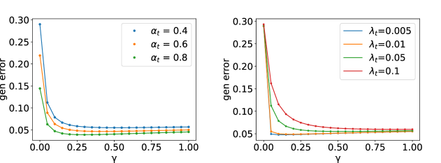
C.2 A simple example of transfer regression

In Figure 4 we show an example of a transfer learning problem in a single-layer, linear version of the task shown in Fig. 2 of the main text, in the special case with two identical teachers for the source and target tasks. We generate the three datasets Xssubscript๐‘‹๐‘ X_{s}, $X_{t}$ and $X_{t}$ with normal i.i.d. entries. The task is defined in terms of a random teacher weight vector $w_{0}$ with zero-mean and Gaussian i.i.d. entries with standard deviation $1/N$ (we use $N=200$ in this examples): outputs for the three sets are linear functions of the inputs $X_{\alpha}$ given by $y_{\alpha}=X_{\alpha}w_{0}$ for ฮฑโˆˆ{s,t,ฯ„}๐›ผ๐‘ ๐‘ก๐œ\alpha\in\left\{s,t,\tau\right\}. The source weight vector wssubscript๐‘ค๐‘ w_{s} is trained using Ps=ฮฑsโ€‹Nsubscript๐‘ƒ๐‘ subscript๐›ผ๐‘ ๐‘P_{s}=\alpha_{s}N data-points, with ฮฑs=0.8subscript๐›ผ๐‘ 0.8\alpha_{s}=0.8. The transfer effect is apparent in the decrease of the generalization error as a function of the source-target coupling parameter $\gamma$.

Refer to caption
Figure 4: Transfer learning in a linear regression task defined by a random teacher vector $w_{0}$. In both panels curves are theoretical results, points are obtained by solving the source and target problem with standard optimization methods. Parameters: $N=200$, $P_{\tau}=10.000$ A: Generalization error as a function of the coupling parameter $\gamma$ for different sizes of the training set for the target problem, indicated by the ratio $\alpha_{t}=P_{t}/N$. B: Same as A for different values of the regularization $\lambda_{t}$ of the target weight vector $w_{t}$.

Appendix D Transfer learning in a deep fully connected network

In this section, we sketch a tentative derivation of the effective action in the case of networks with $L$ hidden layers. In this case, all the layers except for the last are coupled among source and target, while the readout ($L+1$ in our convention) remains uncoupled. The replicated priors for the weights at each layer are defined by the coupling matrices $\Lambda_{l}$:

ฮ›l=(ฮปs,lโˆ’ฮณโˆ’ฮณโ€ฆโˆ’ฮณโˆ’ฮณฮปt,l0โ€ฆ0โˆ’ฮณ0ฮปt,lโ€ฆโ€ฆโ€ฆโ€ฆโ€ฆโ€ฆ0โˆ’ฮณ0โ€ฆ0ฮปt,l),ฮ›L+1=(ฮปs,L+100โ€ฆ00ฮปt,L+10โ€ฆ000ฮปt,L+1โ€ฆโ€ฆโ€ฆโ€ฆโ€ฆโ€ฆ000โ€ฆ0ฮปt,L+1).formulae-sequencesubscriptฮ›๐‘™subscript๐œ†๐‘ ๐‘™๐›พ๐›พโ€ฆ๐›พ๐›พsubscript๐œ†๐‘ก๐‘™0โ€ฆ0๐›พ0subscript๐œ†๐‘ก๐‘™โ€ฆโ€ฆโ€ฆโ€ฆโ€ฆโ€ฆ0๐›พ0โ€ฆ0subscript๐œ†๐‘ก๐‘™subscriptฮ›๐ฟ1subscript๐œ†๐‘ ๐ฟ100โ€ฆ00subscript๐œ†๐‘ก๐ฟ10โ€ฆ000subscript๐œ†๐‘ก๐ฟ1โ€ฆโ€ฆโ€ฆโ€ฆโ€ฆโ€ฆ000โ€ฆ0subscript๐œ†๐‘ก๐ฟ1\Lambda_{l}=\left(\begin{array}[]{ccccc}\lambda_{s,l}&-\gamma&-\gamma&...&-\gamma\\ -\gamma&\lambda_{t,l}&0&...&0\\ -\gamma&0&\lambda_{t,l}&...&...\\ ...&...&...&...&0\\ -\gamma&0&...&0&\lambda_{t,l}\end{array}\right)\,,\qquad\Lambda_{L+1}=\left(\begin{array}[]{ccccc}\lambda_{s,L+1}&0&0&...&0\\ 0&\lambda_{t,L+1}&0&...&0\\ 0&0&\lambda_{t,L+1}&...&...\\ ...&...&...&...&0\\ 0&0&...&0&\lambda_{t,L+1}\end{array}\right)\,. (131)

We are interested in the computation of the replicated partition function $Z^{n}$, using index $a=1\ldots n$ for replicas. To describe a fully connected layer with weight matrix $w_{l}$, we introduce the following notation for the pre-activations at layer $l+1$:

$$h_{l+1}^{a}=w^{a}_{l}x^{a}_{l},\qquad x^{a}_{l}=\sigma\left(h^{a}_{l}\right)\,.$$ (132)

To easily deal with the recursion over layer, let us introduce a definition for the function computed by a neural network between any two intermediate layers $l$, $l^{\prime}$:

$\displaystyle h_{l^{\prime}}^{a}=\phi_{l:l^{\prime}}^{a}\left(h_{l};\left\{w^{a}\right\}_{l+1:l^{\prime}}\right)\,.$ (133)

The function $\phi_{l:l^{\prime}}$ takes as inputs the pre-activations at layer $l$ and outputs the pre-activations at layer $l^{\prime}$, with the convention that $h_{0}=x$. We have stressed the dependence of $\phi_{l:l^{\prime}}$ on all the weights of the layers between $l$ and $l^{\prime}$, $\{w\}_{l+1:l^{\prime}}$, but we will immediately drop it to ease the notation. The output of the network reads $\phi\left(x\right)\equiv\phi_{0:L+1}\left(x\right)$, and we can write the loss in terms of the pre-activations of layer $l$ as:

$$\mathcal{L}\left(\left\{w\right\}\right)=\frac{1}{2}\sum_{\mu}\left(\phi\left(x^{\mu}\right)-y^{\mu}\right)^{2}=\sum_{\mu}\left(\phi_{l:L+1}\left(h_{l}^{\mu}\right)-y^{\mu}\right)^{2}\,.$$ (134)

Let us define:

$$\chi_{l:l^{\prime}}\left(h_{l}^{\mu};\{w\}_{l+1:l^{\prime}}\right)=\exp\left[-\frac{1}{2}\sum_{\mu a}\beta_{a}\left(\phi_{l:l^{\prime}}\left(h_{l}^{\mu}\right)-y_{\mu}^{a}\right)^{2}\right]\,,$$

Using this convention we can rewrite the free-entropy as:

$\displaystyle f$ =1NLโ€‹1Zsโ€‹(ฮฒs)โ€‹limnโ†’0โˆ‚nZnabsent1subscript๐‘๐ฟ1subscript๐‘๐‘ subscript๐›ฝ๐‘ subscriptโ†’๐‘›0subscript๐‘›superscript๐‘๐‘›\displaystyle=\frac{1}{N_{L}}\frac{1}{Z_{s}\left(\beta_{s}\right)}\lim_{n\to 0}\partial_{n}Z^{n} (135)
$\displaystyle Z^{n}$ $\displaystyle=\int\prod_{l}\mathcal{D}w_{l}\,\chi_{0:L+1}(x)e^{-\frac{1}{2}\sum_{l}w_{l}^{T}\Lambda_{l}w_{l}}\,,$ (136)

with the shorthands $\mathcal{D}w_{l}=\prod_{i_{l}i_{l-1},a}dw_{i_{l}i_{l-1}}^{l,a}$ and $w_{l}^{T}\Lambda_{l}w_{l}=\sum_{i_{l}i_{l-1}}\sum_{ab}w_{l,i_{l}i_{l-1}}^{l,a}\Lambda_{l,ab}w_{l,i_{l}i_{l-1}}^{l,b}$.

D.1 Integrating first-layer weights

The integration over the first-layer weights $w^{a}_{1,i_{0}i_{1}}$ is straightforward, since for each $i_{1},i_{0}$ the coupling is Gaussian with inverse covariance $\Lambda_{1}$. Let us isolate the integral over the first-layer weights and consider the dependence over the first layer pre-activations:

$$Z^{n}=\int\prod_{l>1}\mathcal{D}w_{l}e^{-\frac{1}{2}\sum_{l>1}w_{l}^{T}\Lambda_{l}w_{l}}\int\mathcal{D}h_{1}\chi_{1:L+1}\left(h_{1}\right)\psi\left(h_{1}\right)$$ (137)

where:

$$\psi\left(h_{1}\right)=\prod_{i_{1}}\int\prod_{\mu}d\bar{h}_{1,\mu i_{1}}^{a}e^{i\sum_{a\mu}\bar{h}_{1,\mu i_{1}}^{a}h_{1,\mu i_{1}}^{a}}\prod_{i_{0}}\int dwe^{-\frac{1}{2}\sum_{ab}w^{a}\Lambda_{1}^{ab}w^{b}-\frac{i}{\sqrt{N_{0}}}\sum_{a\mu}w^{a}\bar{h}_{1,\mu i_{1}}^{a}x_{\mu i_{0}}^{a}}.$$ (138)

Integrating over the weights and using the notation $\Delta_{l}=\mathrm{exp}\{-\frac{1}{2}N_{l-1}N_{l}\log\det\Lambda_{l}\}$, we have:

$$\psi\left(h_{1}\right)=\Delta_{1}\prod_{i_{1}i_{0}}\int\prod_{\mu}d\bar{h}_{1,\mu i_{1}}^{a}e^{i\sum_{a\mu}\bar{h}_{1,\mu i_{1}}^{a}\bar{h}_{1,\mu i_{1}}^{a}-\frac{1}{2}\sum_{ab}\Lambda_{ab}^{-1}\bar{q}_{0,i_{1}i_{0}}^{a}\left(\bar{h}\right)\bar{q}_{0,i_{1}i_{0}}^{b}\left(\bar{h}\right)}$$ (139)

with the definition

$$\bar{q}_{0,i_{1}i_{0}}^{a}\left(\bar{h}\right)=\frac{1}{\sqrt{N_{0}}}\sum_{\mu}\bar{h}_{\mu i_{1}}^{a}x_{\mu i_{0}}^{a}\,.$$ (140)

Employing the factorization over the first layer index $i_{1}$ and summing over $i_{0}$, we can write the replicated partition function as follows

$$Z^{n}=\Delta_{1}\int\prod_{l>1}\mathcal{D}w_{l}e^{-\frac{1}{2}\sum_{l>1}w_{l}^{T}\Lambda_{l}w_{l}}\int\prod_{i_{1}}\left\{\mathcal{D}h_{1,i_{1}}\mathcal{N}\left(h_{1,i_{1}};0,\Sigma_{1}\right)\right\}\chi_{1:L+1}\left(\left\{h_{1}\right\}_{i_{1}}\right)$$ (141)

where, for each $i_{1}$, the replicated pre-activations are Gaussian with covariance matrices $\Sigma_{1}$:

$$\tilde{C}_{\mu\nu}^{ab}=\left\langle h_{1,\mu i_{1}}^{a}h_{1,\nu i_{1}}^{b}\right\rangle=\left(\Lambda_{1}^{-1}\right)^{ab}C_{\mu\nu}^{ab}$$ (142)

in turn depending on the replicated input covariances:

$$C_{\mu\nu}^{ab}=\frac{1}{N_{0}}\sum_{i_{0}=1}^{N_{0}}x_{\mu i_{0}}^{a}x_{\nu i_{0}}^{b}\,.$$ (143)

D.2 Recursion relation for deep FC network

Introducing the definition for the second-layer pre-activations we have:

$$Z^{n}=\Delta_{1}\int\prod_{l>2}\mathcal{D}w_{l}e^{-\frac{1}{2}\sum_{l>2}w_{l}^{T}\Lambda_{l}w_{l}}\int\mathcal{D}h_{2}\chi_{2:L+1}\left(h_{2}\right)\psi\left(h_{2}\right)$$ (144)

with:

$\displaystyle\psi\left(h_{2}\right)$ $\displaystyle=\int\mathcal{D}\bar{h}_{2}e^{i\bar{h}_{2}^{T}h_{2}}\int\prod_{i_{1}}\left\{\mathcal{D}h_{1,i_{1}}\mathcal{N}\left(h_{1,i_{1}};0,\Sigma_{1}\right)\right\}$
$\displaystyle\int\mathcal{D}w_{2}\prod_{i_{2}i_{1}}e^{-\frac{i}{\sqrt{N_{1}}}\sum_{a}w_{2,i_{2}i_{1}}^{a}\sum_{\mu}\bar{h}_{2,\mu i_{2}}^{a}\sigma\left(h_{1,\mu i_{1}}^{a}\right)}$ (145)

We again introduce the quantities

$$\bar{q}_{1,i_{2}i_{1}}^{a}\left(\bar{h}_{2}\right)=\frac{1}{\sqrt{N_{1}}}\sum_{\mu}\bar{h}_{2,\mu i_{2}}^{a}\sigma\left(h_{1,\mu i_{1}}^{a}\right)$$ (146)

and perform the integration over the weights $w_{2}$. Employing the factorization over the index $i_{1}$ (and dropping the index for clarity) we write

$$\psi\left(h_{2}\right)=\Delta_{2}\prod_{i_{2}i_{1}}\int\mathcal{D}\bar{h}_{2}e^{i\bar{h}_{2}^{T}h_{2}}\left(\int\mathcal{D}\bar{q}_{1}\varphi\left(\bar{q}_{1}\right)e^{-\frac{1}{2}\bar{q}_{1}^{T}\bar{q}_{1}-\frac{1}{2}\bar{q}_{1}^{T}\Lambda_{2}^{-1}\bar{q}_{1}}\right)^{N_{1}}$$ (147)

with:

$$\varphi\left(\bar{q}_{1}\right)=\left\langle\prod_{i_{2}}\delta\left(\bar{q}_{1,i_{2}}^{a}-\frac{1}{\sqrt{N_{1}}}\sum_{\mu}\bar{h}_{2,\mu i_{2}}^{a}\sigma\left(h_{1,\mu}^{a}\right)\right)\right\rangle_{h_{1}}$$ (148)

To deal with the extensive extensive $N_{2}n$ number of variables $\bar{q}_{1}$, we employ a self-consistent Gaussian approximation with covariance matrix

$$\bar{\mathcal{Q}}_{1,i_{2}j_{2}}^{ab}=\left\langle\bar{q}_{1,i_{2}}^{a}\bar{q}_{1,j_{2}}^{b}\right\rangle=\frac{1}{N_{1}}\sum_{\mu\nu}\bar{h}_{2,\mu i_{2}}^{a}K_{1,\mu\nu}^{ab}\bar{h}_{2,\nu j_{2}}^{b}$$ (149)

and kernels

$$K_{1,\mu\nu}^{ab}=\left\langle\sigma\left(h_{1,\mu}^{a}\right)\sigma\left(h_{1,\nu}^{ab}\right)\right\rangle_{\mathcal{N}\left(h_{1};0,\tilde{C}\right)}$$ (150)

thus getting:

$\displaystyle\left\langle e^{-\frac{1}{2}\bar{q}_{1}^{T}\Lambda_{2}^{-1}\bar{q}_{1}}\right\rangle_{\varphi\left(\bar{q}_{1}\right)}$ $\displaystyle=e^{-\frac{N_{1}}{2}\mathop{}\!\mathrm{Tr}_{i_{2},a}\log\left(\mathbb{1}+\left(\Lambda_{2}^{-1}\right)^{ab}\bar{\mathcal{Q}}_{1,i_{2}j_{2}}^{ab}\right)}\sim$
$\displaystyle e^{-\frac{N_{1}}{2}\mathop{}\!\mathrm{Tr}_{a}\log\left(\mathbb{1}+\left(\Lambda_{2}^{-1}\right)^{ab}\mathop{}\!\mathrm{Tr}_{i_{2}}\bar{\mathcal{Q}}_{1,i_{2}j_{2}}^{ab}\right)}$ (151)

The second line of the previous equations implement a mean-field, permutation symmetric approximation, whereby we obtained an inter-replica covariance by tracing over the $N_{2}$ second-layer hidden units.

Introducing the definitions for the new mean-field inter-replica covariance with appropriate $\delta$ functions, we thus get:

$\displaystyle\psi\left(h_{2}\right)$ $\displaystyle=\Delta_{2}\int\mathcal{D}\mathcal{\bar{Q}}_{1}e^{-\frac{1}{2}\log\det\left(\mathbb{1}+\Lambda_{2}^{-1}\mathcal{\bar{Q}}_{1}\right)}$
$\displaystyle\int\mathcal{D}\bar{h}e^{i\bar{h}^{T}h_{2}}\delta\left(N_{1}\mathcal{\bar{Q}}_{1}^{ab}-\left(\bar{h}^{a}\right)^{T}K_{1}^{ab}\bar{h}^{b}\right)$ (152)

Expanding the $\delta$โ€™s and easily integrating over $\bar{h}$ we find:

$$\psi\left(h_{2}\right)=\Delta_{2}\int\mathcal{D}\mathcal{Q}_{1}\mathcal{D}\bar{\mathcal{Q}}_{1}e^{\frac{N_{1}}{2}\mathop{}\!\mathrm{Tr}\left(\mathcal{Q}_{1}\mathcal{\bar{Q}}_{1}\right)-\frac{1}{2}\log\det\left(\mathbb{1}+\Lambda_{2}^{-1}\mathcal{\bar{Q}}_{1}\right)}\mathcal{N}\left(h_{2};0,\mathcal{K}_{2}\right)$$ (153)

with

$$\mathcal{K}_{2}^{ab}=\mathcal{Q}_{1}^{ab}K_{1}^{ab}$$ (154)

The matrix $\mathcal{Q}_{1}$ acts as renormalization for the kernel $K_{1}$, whereby $h_{2}$ are Gaussian conditioning on $\mathcal{Q}_{1}$. Using a simple recursion across layer one gets:

$\displaystyle Z^{n}$ $\displaystyle=\prod_{l=1}^{L}\Delta_{l}\int\prod_{l=1}^{L-1}\mathcal{D}\mathcal{Q}_{l}\mathcal{D}\bar{\mathcal{Q}}_{l}e^{\frac{1}{2}\sum_{l=1}^{L-1}N_{l}\mathop{}\!\mathrm{Tr}\left(\mathcal{Q}_{l}\mathcal{\bar{Q}}_{l}\right)-\frac{1}{2}\sum_{l=1}^{L-1}\log\det\left(\mathbb{1}+\Lambda_{l+1}^{-1}\mathcal{\bar{Q}}_{l}\right)}$
$\displaystyle\int\mathcal{D}ve^{-\frac{1}{2}v^{T}\Lambda_{L+1}v}\int\mathcal{D}h^{L}\chi_{L:L+1}\left(h^{L}\right)\psi\left(h^{L}\right)$ (155)

with the notation $v\equiv w_{L+1}$ on the uncoupled last layer weights.

D.3 Readout layer

Introducing the definition s=ฯ•L:L+1โ€‹(hL;v)๐‘ subscriptitalic-ฯ•:๐ฟ๐ฟ1subscriptโ„Ž๐ฟ๐‘ฃs=\phi_{L:L+1}\left(h_{L};v\right) for the readout outputs, we obtain a form

Zn=โˆl=1Lฮ”lโ€‹โˆซโˆl=1Lโˆ’1๐’Ÿโ€‹๐’ฌlโ€‹๐’Ÿโ€‹๐’ฌยฏlโ€‹e12โ€‹โˆ‘l=1Lโˆ’1Nlโ€‹Trโ€‹(๐’ฌlโ€‹๐’ฌยฏl)โˆ’12โ€‹โˆ‘l=1Lโˆ’1logโ€‹det(๐Ÿ™+ฮ›l+1โˆ’1โ€‹๐’ฌยฏl)โ€‹โˆซ๐’Ÿโ€‹sโ€‹ฯˆโ€‹(s)superscript๐‘๐‘›superscriptsubscriptproduct๐‘™1๐ฟsubscriptฮ”๐‘™superscriptsubscriptproduct๐‘™1๐ฟ1๐’Ÿsubscript๐’ฌ๐‘™๐’Ÿsubscriptยฏ๐’ฌ๐‘™superscript๐‘’12superscriptsubscript๐‘™1๐ฟ1subscript๐‘๐‘™Trsubscript๐’ฌ๐‘™subscriptยฏ๐’ฌ๐‘™12superscriptsubscript๐‘™1๐ฟ1double-struck-๐Ÿ™superscriptsubscriptฮ›๐‘™11subscriptยฏ๐’ฌ๐‘™๐’Ÿ๐‘ ๐œ“๐‘ Z^{n}=\prod_{l=1}^{L}\Delta_{l}\int\prod_{l=1}^{L-1}\mathcal{D}\mathcal{Q}_{l}\mathcal{D}\bar{\mathcal{Q}}_{l}e^{\frac{1}{2}\sum_{l=1}^{L-1}N_{l}\mathop{}\!\mathrm{Tr}\left(\mathcal{Q}_{l}\mathcal{\bar{Q}}_{l}\right)-\frac{1}{2}\sum_{l=1}^{L-1}\log\det\left(\mathbb{1}+\Lambda_{l+1}^{-1}\mathcal{\bar{Q}}_{l}\right)}\int\mathcal{D}s\psi\left(s\right) (156)

with

ฯˆโ€‹(s)๐œ“๐‘ \displaystyle\psi\left(s\right) =ฮ”L+1โ€‹โˆซ๐’Ÿโ€‹sยฏโ€‹eiโ€‹sยฏTโ€‹sโˆ’12โ€‹(sโˆ’y)Tโ€‹Bโ€‹(sโˆ’y)โ€‹โˆซ๐’Ÿโ€‹hLโ€‹๐’ฉโ€‹(hL;0,๐’ฆL)absentsubscriptฮ”๐ฟ1๐’Ÿยฏ๐‘ superscript๐‘’๐‘–superscriptยฏ๐‘ ๐‘‡๐‘ 12superscript๐‘ ๐‘ฆ๐‘‡๐ต๐‘ ๐‘ฆ๐’Ÿsubscriptโ„Ž๐ฟ๐’ฉsubscriptโ„Ž๐ฟ0subscript๐’ฆ๐ฟ\displaystyle=\Delta_{L+1}\int\mathcal{D}\bar{s}e^{i\bar{s}^{T}s-\frac{1}{2}\left(s-y\right)^{T}B\left(s-y\right)}\int\mathcal{D}h_{L}\mathcal{N}\left(h_{L};0,\mathcal{K}_{L}\right)
โˆซ๐’Ÿโ€‹vโ€‹โˆiLeโˆ’iNLโ€‹โˆ‘aviLaโ€‹โˆ‘ฮผsยฏฮผaโ€‹ฯƒโ€‹(hL,ฮผโ€‹iLa)๐’Ÿ๐‘ฃsubscriptproductsubscript๐‘–๐ฟsuperscript๐‘’๐‘–subscript๐‘๐ฟsubscript๐‘Žsuperscriptsubscript๐‘ฃsubscript๐‘–๐ฟ๐‘Žsubscript๐œ‡superscriptsubscriptยฏ๐‘ ๐œ‡๐‘Ž๐œŽsuperscriptsubscriptโ„Ž๐ฟ๐œ‡subscript๐‘–๐ฟ๐‘Ž\displaystyle\int\mathcal{D}v\prod_{i_{L}}e^{-\frac{i}{\sqrt{N_{L}}}\sum_{a}v_{i_{L}}^{a}\sum_{\mu}\bar{s}_{\mu}^{a}\sigma\left(h_{L,\mu i_{L}}^{a}\right)} (157)

We again introduce the variables qยฏa=1NLโ€‹โˆ‘ฮผsยฏฮผaโ€‹ฯƒโ€‹(hL,ฮผa)superscriptยฏ๐‘ž๐‘Ž1subscript๐‘๐ฟsubscript๐œ‡superscriptsubscriptยฏ๐‘ ๐œ‡๐‘Ž๐œŽsuperscriptsubscriptโ„Ž๐ฟ๐œ‡๐‘Ž\bar{q}^{a}=\frac{1}{\sqrt{N_{L}}}\sum_{\mu}\bar{s}_{\mu}^{a}\sigma\left(h_{L,\mu}^{a}\right), where we dropped the index $i_{L}$ owning to factorization. Employing the usual Gaussian equivalence, their joint distribution is a normal distribution with order-parameter covariance matrix

๐’ฌยฏLaโ€‹b=โŸจqยฏaโ€‹qยฏbโŸฉ=1NLโ€‹(sยฏa)Tโ€‹KLaโ€‹bโ€‹sยฏbsuperscriptsubscriptยฏ๐’ฌ๐ฟ๐‘Ž๐‘delimited-โŸจโŸฉsuperscriptยฏ๐‘ž๐‘Žsuperscriptยฏ๐‘ž๐‘1subscript๐‘๐ฟsuperscriptsuperscriptยฏ๐‘ ๐‘Ž๐‘‡superscriptsubscript๐พ๐ฟ๐‘Ž๐‘superscriptยฏ๐‘ ๐‘\bar{\mathcal{Q}}_{L}^{ab}=\left\langle\bar{q}^{a}\bar{q}^{b}\right\rangle=\frac{1}{N_{L}}\left(\bar{s}^{a}\right)^{T}K_{L}^{ab}\bar{s}^{b} (158)

and kernels

$$K_{L,\mu\nu}^{ab}=\left\langle\sigma\left(h_{\mu}^{a}\right)\sigma\left(h_{\nu}^{a}\right)\right\rangle_{\mathcal{N}\left(h_{L};0,\mathcal{K}_{L}\right)}$$ (159)

We finally obtain

ฯˆโ€‹(s)๐œ“๐‘ \displaystyle\psi\left(s\right) $\displaystyle=\Delta_{L+1}\int\mathcal{D}\mathcal{Q}_{L}\mathcal{D}\bar{\mathcal{Q}}_{L}e^{\frac{N_{L}}{2}\mathop{}\!\mathrm{Tr}\left(\mathcal{Q}_{L}\mathcal{\bar{Q}}_{L}\right)-\frac{1}{2}\log\det\left(\mathbb{1}+\Lambda_{L+1}^{-1}\mathcal{\bar{Q}}_{L}\right)}$
โˆซ๐’Ÿโ€‹sยฏโ€‹eiโ€‹sยฏTโ€‹sโˆ’12โ€‹sยฏTโ€‹๐’ฆL+1โ€‹sยฏโˆ’12โ€‹(sโˆ’y)Tโ€‹Bโ€‹(sโˆ’y)๐’Ÿยฏ๐‘ superscript๐‘’๐‘–superscriptยฏ๐‘ ๐‘‡๐‘ 12superscriptยฏ๐‘ ๐‘‡subscript๐’ฆ๐ฟ1ยฏ๐‘ 12superscript๐‘ ๐‘ฆ๐‘‡๐ต๐‘ ๐‘ฆ\displaystyle\int\mathcal{D}\bar{s}e^{i\bar{s}^{T}s-\frac{1}{2}\bar{s}^{T}\mathcal{K}_{L+1}\bar{s}-\frac{1}{2}\left(s-y\right)^{T}B\left(s-y\right)} (160)

where $\mathcal{K}_{L+1}^{ab}=\mathcal{Q}_{L}^{ab}K_{L}^{ab}$. We now employ the same steps as in the case of the 1hl network, thus arriving at the final form

$$Z^{n}=\int\prod_{l}\mathcal{D}\mathcal{Q}_{l}\mathcal{D}\bar{\mathcal{Q}}_{l}e^{\frac{N_{L}}{2}S\left(\mathcal{Q},\mathcal{\bar{Q}}\right)}$$ (161)

with the action

$\displaystyle S$ $\displaystyle=\sum_{l}^{L}\left[\log\Delta_{l}+\frac{N_{l}}{N_{L}}\mathop{}\!\mathrm{Tr}\left(\mathcal{Q}_{l}\mathcal{\bar{Q}}_{l}\right)-\frac{N_{l}}{N_{L}}\sum_{l}\log\det\left(\mathbb{1}+\Lambda_{l+1}^{-1}\mathcal{\bar{Q}}_{l}\right)\right]+$
$\displaystyle\log\Delta_{L+1}-\log\det\left(\mathbb{1}+B\mathcal{K}_{L+1}\right)-y^{T}\left(B^{-1}+\mathcal{K}_{L+1}\right)^{-1}y\,.$ (162)

The $n\to 0$ limit can again be carried out using the expressions for the determinants and quadratic forms in section B.6. It is worth noticing that we expect this derivation to be exact for deep linear networks, as long as replica symmetry is not broken.

Appendix E Details of numerical experiments

In this section, we provide some details about training algorithm and tasks used for numerical validation of our theoretical results. All experiments are performed on pairs of source/target architectures with one hidden layer and Erf (error function) activation. To ensure sampling from the posterior Gibbs ensemble of weights, which is essential to validate our theory, we train our networks using a discretised Langevin dynamics, similarly to what is done in [26, 23, 30, 33]. At each training step $t$, the parameters $\theta=\{w,v\}$ are updated according to:

$$\theta(t+1)=\theta(t)-\eta\nabla_{\theta}\tilde{\mathcal{L}}(\theta(t))+\sqrt{2T\eta}\epsilon(t)$$ (163)

where $T=1/\beta$ is the temperature, $\eta$ is the learning rate, $\epsilon(t)$ is a white Gaussian noise vector with entries drawn from a standard normal distribution, and the regularized loss function $\tilde{\mathcal{L}}$ comprises the prior rescaled by the temperature:

โ„’~s/t=โ„’s/t+Tโ€‹ฮปs/t,12โ€‹โ€–ws/tโ€–2+Tโ€‹ฮปs/t,22โ€‹โ€–vs/tโ€–2.subscript~โ„’๐‘ ๐‘กsubscriptโ„’๐‘ ๐‘ก๐‘‡subscript๐œ†๐‘ ๐‘ก12superscriptnormsubscript๐‘ค๐‘ ๐‘ก2๐‘‡subscript๐œ†๐‘ ๐‘ก22superscriptnormsubscript๐‘ฃ๐‘ ๐‘ก2\tilde{\mathcal{L}}_{s/t}=\mathcal{L}_{s/t}+\frac{T\lambda_{s/t,1}}{2}\|w_{s/t}\|^{2}+\frac{T\lambda_{s/t,2}}{2}\|v_{s/t}\|^{2}. (164)

Temperature and learning rate are fixed to $T=10^{-2}$ and $\eta=10^{-3}$ throughout the experiments for both source and target networks.

E.1 Experimental Setup

We use pairs of correlated source/task classification tasks. Two pairs involve real-world computer vision datasets (C-EMNIST and C-CIFAR), and one is a synthetic task (CHMM). We train the source model on the source task first, then extract $k$ equilibrium configurations of the source weights. For each of the $k$ sets of features, we train a target network for different values of the parameter $\gamma$ controlling the coupling to source weights, and average results over the $k$ source configurations. In Fig.ย 1 of the main text $k=5$, in Fig. 2 we used $k=10$.

E.1.1 C-EMNIST and C-CIFAR

Similarly toย [11], we build a binary source task by dividing a subset of the EMNIST letters into two distinct groups: letters $\{A,B,E,L\}$ for the first one and $\{C,H,J,S\}$ for the second one. We assign the label to each image according to the group membership. The target task is then built from the source task by replacing one letter per group (letter $E$ with $F$ and $J$ with $I$). We call this pair of source/target tasks C-EMNIST (correlated EMNIST). C-CIFAR is constructed in a similarly way from the CIFAR10 dataset: the source task includes the first $8$ classes, specifically $\{1,2,3,4\}$ in the first group and $\{5,6,7,8\}$ in the second one. The target task is obtained by replacing class $1$ with $10$ and class $5$ with $9$).

In all experiments, images from CIFAR10 and EMNIST are gray-scaled and down-sized. In Fig. 2 and 3 of the main text, the input size is set to $N_{0}=784$ pixels. in Fig. 1B, the curves at $N_{1}=500$ have $N_{0}=784$, while those at $N_{1}=1000$ are obtained by pre-processing the input data points $x$ with random features:

$$\hat{x}=\sigma\left(\frac{Fx}{N_{0}}\right)$$ (165)

where $F\in\mathbb{R}^{D\times N_{0}}$ is the random feature matrix, whose entries are sampled iid from a standard Gaussian. This effectively projects the input data points in a new space of dimension $D$. In the experiments in fig.ย 1B we set $D=400$.

E.1.2 CHMM

To analyze the extent to which the correlation between source/target tasks is essential for TL to be beneficial, we use the correlated hidden manifold (CHMM), a synthetic data model where source-target correlations can be explicitly tuned via three different set of parameters, meant to mimic different and realistic TL scenarios [11].

For instance, the source and the target set may differ because of the traits characterizing the input data point. In the model, this is described via the parameters $\rho$ and $\eta$ which control, respectively, how many features of the source data are replaced by new ones in the target set and how much the remaining features differ between the two tasks. The source-target datasets may instead share the same set of input data but these data could be labelled according to different labelling rules. The mismatch between the labelling rules is controlled via the parameter $q$. Finally, the source-target datasets may differ in terms of the dimensionality of the data manifold, which can be controlled by directly tuning the source and target intrinsic dimensions.