Frequency and Generalisation of Periodic Activation Functions in Reinforcement Learning

Abstract

Periodic activation functions, often referred to as learned Fourier features have been widely demonstrated to improve sample efficiency and stability in a variety of deep RL algorithms. Potentially incompatible hypotheses have been made about the source of these improvements. One is that periodic activations learn low frequency representations and as a result avoid overfitting to bootstrapped targets. Another is that periodic activations learn high frequency representations that are more expressive, allowing networks to quickly fit complex value functions. We analyse these claims empirically, finding that periodic representations consistently converge to high frequencies regardless of their initialisation frequency. We also find that while periodic activation functions improve sample efficiency, they exhibit worse generalization on states with added observation noise—especially when compared to otherwise equivalent networks with ReLU activation functions. Finally, we show that weight decay regularization is able to partially offset the overfitting of periodic activation functions, delivering value functions that learn quickly while also generalizing.

1 Introduction

Deep learning has enabled reinforcement learning (RL) to conquer environments with large, high dimensional state spaces (e.g. Silver et al. (2016); Badia et al. (2020)). The architectures of deep RL agents have largely emulated innovations from supervised learning—a prime example being the original deep Q-networks (Silver et al., 2013), which used the GPU-optimized implementation of convolutional layers from AlexNet (Krizhevsky et al., 2012). However, design choices inherited from supervised learning do not always readily meet the demands of RL. For example, popular techniques such as weight decay (Salimans & Kingma, 2016) and momentum (Bengio et al., 2021) do not improve performance in RL as consistently as they do in the supervised learning contexts in which they were initially developed.

One important dimension along which RL differs from supervised learning is in the trade-off between generalization and memorization, with RL algorithms often benefiting from localized features (Ghiassian et al., 2020) such as tile coding (Sherstov & Stone, 2005), which limit the degree to which the function approximator can generalize updates on one state’s predicted value to other distant states. While some degree of generalization is necessary for large problem scales, it is desirable to be able to calibrate the spectral bias of a function approximator to a particular problem instance. Fourier features, a popular representation for both supervised learning (Rahimi & Recht, 2007) as well as linear RL (Konidaris et al., 2011), present one means of achieving this objective, whereby the degree of generalization between training samples of the ensuing linear function approximator can be precisely specified by the frequency with which these features are initialized. Low-frequencies bias the learner towards smooth functions that generalize more between training samples, whereas high-frequencies will bias the learner towards non-smooth functions.

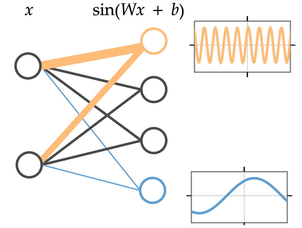
(a)

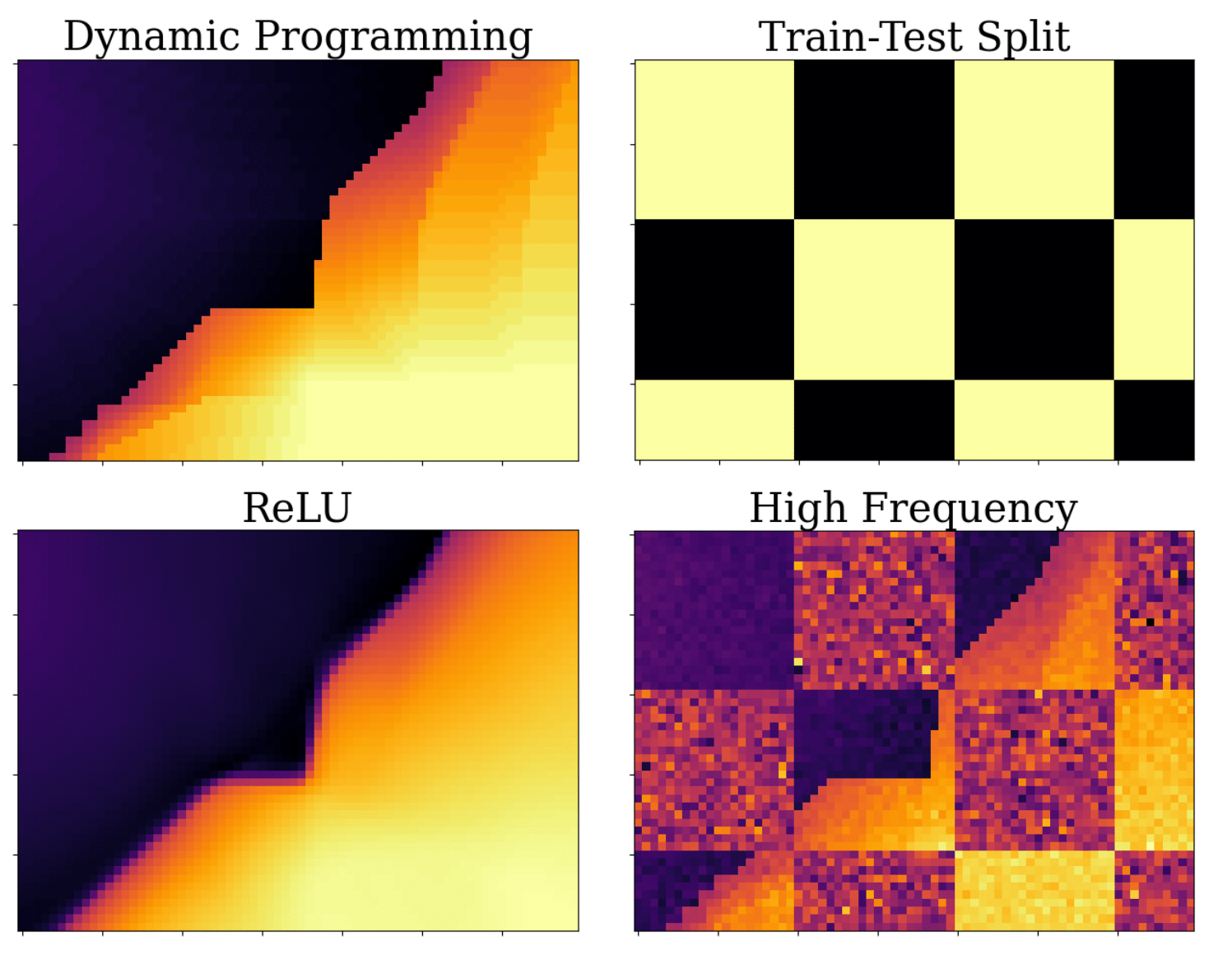
(b)

Figure 1: (a) Learned Fourier feature layer are fully-connected layers with a $\sin$ activation. Larger weights lead to faster oscillations. (b) High frequency Fourier features predict accurately in distribution but do not generalize. Top left is a segment of the ground truth value function from the mountain car environment (Moore, 1990), top right shows the training/test distributions: light is train, dark is test. Using supervised learning to fit the ground truth value function with a ReLU network (bottom left) and a Fourier feature network (bottom right), see appendix A.1 for details.

Prior to the widespread adoption of deep RL, the Fourier features used in RL consisted of a vector of stacked Fourier decompositions of each state variable (where each state variable is decomposed into range of different frequencies), which are then fed to a linear function approximator (Konidaris et al., 2011). This approach is difficult to scale to high dimensional inputs as the number of features scales exponentially with the size of the input (see Brellmann et al. (2023) for work on scaling these traditional Fourier features to deep RL tasks). More recently, a more scalable approach has emerged for learning periodic representations, which adds periodic activation functions to neural network architectures (Sitzmann et al., 2020). These periodic activation functions can be viewed as a form of learned Fourier features, replacing the randomly generated, fixed weights of Rahimi & Recht (2007) with trainable parameters.

Li & Pathak (2021) and Yang et al. (2022) applied periodic activations to deep RL, incorporating them into a neural network architecture trained to perform value function approximation. Yang et al. (2022) argue that the use of a periodic activation functions improves sample efficiency because it causes networks to learn high frequency representations that quickly fit high frequency details in value functions. Concurrently, Li & Pathak (2021) also employed periodic activations but with a different perspective. Li & Pathak (2021) state that periodic activations learn low frequency representations, which improves sample efficiency by reducing the amount of overfitting to noisy targets. It is not clear why both works see similar improvements on the same benchmark environments when Yang et al. (2022) suggests that high frequency representations are useful while Li et al. (2020) argues that low frequencies are beneficial.

We investigate how previous works with similar methodologies can arrive at these different conclusions. We are motivated by a simple question: do learned Fourier features help in deep RL because they learn high-frequency representations, or because they learn low-frequency representations? Our findings are summarized as follows: first, we observe the frequency of representations throughout training, finding that they converge to high frequency representations regardless of their initialisation frequency. This growth in frequency can largely be attributed to the growth of the network’s parameter norm, a widely-observed phenomenon in deep reinforcement learning (Nikishin et al., 2022; Dohare et al., 2023). In section 4.2, we show that these high-frequency features result in less robust policies, finding that when noise is added to state observations of the learned Fourier representations they perform worse than ReLU networks. In section 4.3 we connect feature frequency with policy instability, finding that the learned Fourier features are much more sensitive to changes in their input than ReLU features and exhibit a higher effective rank. In section 4.4, we show that weight decay regularisation helps to avoid runaway frequency growth, allowing for use to learn Fourier features which train quickly but also more robust to pertubations in input observations.

2 Related Work

Periodic representations are widely applicable across different domains of machine learning research. In computer vision (Sitzmann et al., 2020; Tancik et al., 2020) Fourier-like positional encodings are used when constructing 3D scenes from 2D images (Mildenhall et al., 2021). For solving partial differential equations, neural Fourier operators learn representations that operate at a range of resolutions (Li et al., 2020). Additionally, geometric deep learning often operates in Fourier space (Cohen et al., 2018; Cobb et al., 2020). Even when not explicitly engineered into an architecture, Fourier features have emerged in transformer architectures (Nanda et al., 2023). Rahimi & Recht (2007) show that even random Fourier features can provide a useful approximation for kernel methods in supervised learning.

In RL, Fourier features were initiated by Konidaris et al. (2011), who learn a value function on top of a fixed Fourier decomposition of each individual variable in the state space. These classic Fourier features has proven to be useful for generalisation in spatial navigation tasks (Yu et al., 2020). Recently, Li & Pathak (2021) and Yang et al. (2022) developed a scalable approach for learning periodic features—achieving state of the art results at the time of publication. A drawback of Fourier representations is that they continue to oscillate outside of their training distribution, leading to inaccurate extrapolation behaviour. More localized feature representations such as tile coding (Sherstov & Stone, 2005) can avoid this extrapolation behaviour. Ghiassian et al. (2020) leveraged localized feature representations to demonstrate the importance of fitting discontinuous local components of the value function for the overall performance and robustness of reinforcement learning algorithms. While localized representations have found some success  (Whiteson, 2010), they have not seen widespread adoption into neural network architectures to the same degree as periodic activations, whose use in neural networks goes back several decades (McCaughan, 1997).

Generalisation in deep reinforcement learning is a more nuanced property than in supervised learning due to its effect on the stability of RL algorithms (van Hasselt et al., 2018). Generalisation between observations in a single environment is a double-edged sword, bringing the potential of accelerating gradient-based optimization methods (Jacot et al., 2018) but also the risk of over-estimation and divergence of the bootstrapped training objective (Achiam et al., 2019). Many works studying generalisation in deep reinforcement learning typically focus on out-of-distribution transfer to new tasks, either drawn from some iid distribution (Cobbe et al., 2019), or obtained by changing the reward (Dayan, 1993; Kulkarni et al., 2016) or some latent factor of the environment transition dynamics. For a comprehensive review of generalisation in reinforcement learning, we refer to the work of Kirk et al. (2023). Our interest will be in the relationship between low-frequency representations and generalization within a single environment, a connection studied in the RL context by Lyle et al. (2022). Relevant to the conclusions of this work, periodic representations in mice have been shown to shift to lower frequencies in states of high levels of uncertainty (Barry et al., 2007).

3 Reinforcement Learning with Periodic Activations

Reinforcement learning is formalised in the framework of Markov decision processes, which are a tuple $\mathcal{M}={\langle\mathcal{S},\mathcal{A},\mathcal{R},\mathcal{P},\gamma\rangle}$ where $\mathcal{S}$ is the set of all states an agent can experience; $\mathcal{A}$ is the set of actions an agent can take; $\mathcal{R}:\mathcal{S}\times\mathcal{A}\rightarrow\mathbb{R}$ is a reward function that gives rewards to the agent; $\gamma\in[0,1]$ is the discount factor that controls how preferential near term rewards are to long term rewards and $\mathcal{P}:\mathcal{S}\times\mathcal{R}\times\mathcal{S}\times\mathcal{A}\rightarrow[0,1]$ is the transition function, where $\mathcal{P}(s^{\prime},r,s,a)=P(S_{t}=s^{\prime},R_{t}=r|S_{t-1}=s,A_{t-1}=a)$, for $S_{t}\in\mathcal{S}$, $A_{t}\in\mathcal{A}$ and $t$ indexes the timestep (Sutton & Barto, 2018, p. 47). This work focuses on episodic reinforcement learning where an agent’s goal is to maximize its expected return $G=\mathbb{E}_{\pi}[\sum_{k=0}^{T}\gamma^{k}r_{t+k+1}]$ in a given episode, where $T$ is the length of the episode and $\pi:\mathcal{S}\rightarrow\mathcal{A}$ is a policy that controls how the agent selects its actions.

Sample efficient neural networks for continuous control are off-policy and actor-critic based, meaning they learn a policy function and an action-value function. Action-value functions $Q:\mathcal{S}\times\mathcal{A}\rightarrow\mathbb{R}$ predict the expected future return given the current state and action $Q(s,a)=\mathbb{E}_{\pi}\left[G_{t}|S_{t}=s,A_{t}=a\right]$ (Sutton & Barto, 2018, p. 58). However, learned Fourier features have only been shown to significantly improve performance when used within the value functions of actor-critic architectures (Li & Pathak, 2021; Yang et al., 2022), and hence we focus our experiments on value learning.

3.1 Representation Frequency

Throughout this work we describe representations as having a frequency. To avoid ambiguity we define the frequency of representations here.

Definition 3.1.

Given a dataset of network inputs $\mathcal{D}$ and layer weights $\mathbf{W}$, the representation frequency $f$ of the $i^{th}$ neuron is the maximum activation minus the minimum activation, divided by $2\pi$. This definition corresponding to the number of wavelengths covered by the $i^{th}$ activation over the dataset $\mathcal{D}$.

$$f_{i}=\left[\frac{\max_{\mathbf{x}\in\mathcal{D}}{\left[(\mathbf{W}\mathbf{x})_{i}\right]}-\min_{\mathbf{x}\in\mathcal{D}}\left[({\mathbf{W}\mathbf{x}})_{i}\right]}{2\pi}\right]$$ (1)

Intuitively, one can plot the activation of a given neuron for different network inputs, which traces out either a sine or cosine wave depending on the choice of periodic activation function. As weight values become larger, the number of periods covered a periodic activation increases. Our definition follow this intuition, counting how many wavelengths the activation oscillates through in the over a dataset of inputs.

Next, we describe the two different flavours of learned Fourier feature architectures from the literature that we call learned Fourier features (Yang et al., 2022) and concatenated learned Fourier features (Li & Pathak, 2021). It is important to note these are equivalent to traditional deep RL architectures, except that they replace activation functions with a sinusoid and/or cosine activation. They do not perform a Fourier decomposition of each state variable as is done by (Konidaris et al., 2011).

3.2 Learned Fourier Features

The learned Fourier features (LFF) of Yang et al. (2022) learn a value function that has a multi-layer perceptron architecture. The first layer of learned Fourier feature networks take the following form $\mathcal{F}=\sin(\mathbf{W}\mathbf{x}+\mathbf{b})$, where $\mathbf{W}$ and $\mathbf{b}$ are weights and biases and $\mathbf{x}$ is the layer input. Then, layers of additional weights and biases are stacked on top of the initial Fourier layer—these subsequent layers have ReLU activations. We denote the ReLU layers as $\mathcal{L}$, meaning an $N$-layer learned Fourier feature value function be written as $Q(s,a)=\mathcal{L}_{N}(\mathcal{L}_{N-1}(...(\mathcal{F}_{1}(s,a)))$, where the state vector $s$ and the action vector $a$ are concatenated into one large vector $x$, which is the input to the learned Fourier feature layer. Yang et al. (2022) initialise weights from a normal distribution and their biases from a uniform distribution, which using their notation, is formulated as the following.

$$\mathbf{W}_{i,j}\sim\mathcal{N}(0,\frac{\pi\beta}{d})$$ (2) $$\mathbf{b}_{j}\sim\mathcal{U}(-\pi,\pi)$$ (3)

Where $\beta$ is the initial bandwidth and $d$ is the dimension of the layer input. Larger weight values $\mathbf{W}_{ij}$ mean higher frequency oscillations in the output neurons as you move through the state space, while smaller weights mean lower frequency oscillations. The bias $\mathbf{b}_{j}$ can be thought of as controlling the phase of the output neurons in the first layer, translating the representation along the output oscillations of each individual neuron. Yang et al. (2022) hypothesise that this architecture allows networks to learn high frequency representations, which prevents the underfitting of value functions that may happen if the first layer uses a ReLU activation.

3.3 Concatenated Learned Fourier Features

Li & Pathak (2021) concatenate the feature input alongside periodic representations in the first layer of their networks. In addition, Li & Pathak (2021) use both cosine and sine activations and concatenate these features into one large vector, which additionally includes the raw state input.

$$\mathcal{CF}=(\sin(\mathbf{W}\mathbf{x}),\cos(\mathbf{W}\mathbf{x}),\mathbf{x})$$ (4)

Where the comma denotes concatenation of $\sin(\mathbf{W}\mathbf{x})$, $\cos(\mathbf{W}\mathbf{x})$ and $\mathbf{x}$ into one larger vector. Note that Li & Pathak (2021) do not include a bias term in their layer architecture. The rest of the architecture follows the same pattern as learned Fourier features with ReLU layers following the initial layer as follows: $Q(s,a)=\mathcal{L}_{N}(\mathcal{L}_{N-1}(...(\mathcal{CF}_{1}(s,a)))$. The motivation of Li & Pathak (2021) was to avoid overfitting to noise in bootstrapped targets when fitting the value function. It was hypothesised that concatenated learned Fourier features would learn smooth representations, while the concatenated $x$ input would retain the high frequency information for the rest of the network.

4 Experiments

Here we empirically investigate the representations of periodic activation functions introduced in section 3 focusing on DeepMind control (Tassa et al., 2018), a standard benchmark for continuous control consisting of a variety of agent morphologies (quadrupeds, fingers and humanoids) paired with reward functions that encourage skills like running or walking. We focus on control from proprioceptive observations. The action space is a continuous vector of forces to apply to different joints. The full set of environments used and hyperparameters used can be found in appendix A.2. Our code builds upon the jaxrl repository (Bradbury et al., 2018; Kostrikov, 2021) with reference to the original repositories of Li et al. (2020) and Yang et al. (2022).

Li & Pathak (2021) and Yang et al. (2022) agree that periodic activation functions are most useful for off-policy algorithms. Furthermore, ablations have shown periodic activations are only beneficial when added to the critic function of actor-critic architectures Li et al. (2020); Yang et al. (2022). As a result, we experiment with periodic activation functions embedded within critic networks only, which themselves are embedded in a soft-actor critic learning algorithm (Haarnoja et al., 2018).

Following Yang et al. (2022), we use a learned Fourier feature critic with a first layer width equal to 40 times the size of the input, followed by two ReLU activated hidden layers of width 1024. The concatenated learned Fourier features critic has an initial layer with the same total width. The ReLU critic has an equivalent architecture except with a ReLU used instead of a periodic activation. All agents have the same actor architecture (details in appendix A.2.2).

4.1 Representation Frequency and In-Distribution Performance

We analyse representation frequency on three environments highlighted by Yang et al. (2022): hopper-hop, walker-run and quadruped-run (we only focus on 3 environments initially due to computational limits, in later sections we broaden our analysis to all 8 environments tested by Yang et al. (2022)). We reproduce the results of both Yang et al. (2022) and Li & Pathak (2021), showing that both approaches are more sample efficient than ReLU architectures on these initial environments. In figure 2(a), we evaluate performance at 100k frames of experience for the walker-run environment at variety of scales $\beta$ (roughly when the improved performance of learned Fourier is most apparent). We measure performance for a range of different initialisation scales $\beta$ (see equation 2).

For low initial scales, learned Fourier features and concatenated learned Fourier features outperform the ReLU baseline (in the low sample limit shown in figure 2(a)). The performance of the Fourier feature architectures is relatively consistent for low initial $\beta$. If very high scale initialisations are used ($\beta>0.03$, roughly equal to $-0.5$ on the x-axis of figure 2(a) and figure 2(b)), the performance of the periodic activations drop dramatically. Furthermore, the performance of learned Fourier features relative to concatenated learned Fourier features is roughly comparable—regardless of initialisation scales. We measure the weight scales and performances for the two additional environments in appendix A.3.

4.1.1 Representation Frequencies After Training

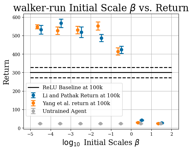
(a)

(b)

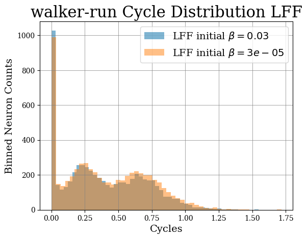
(c)

Figure 2: Regardless of initialisation, learned Fourier features converge to high frequencies. (a) shows return early in training with different initial $\beta$’s. (b) shows how $\beta$ changes through training. (c) shows the distribution of cycles (which is proportional to $\beta$) for different initial $\beta$’s.

We measure weight scales $\beta$ after training by assuming the weight distribution is a diagonal Gaussian, and then computing its standard deviation to extract $\beta$ (see equation 2). Previously, it was hypothesised that lower initial $\beta$’s would lead to lower frequency representations after training, which could improve generalization (Li & Pathak, 2021).

Weight distributions generally rise to similar scales after training regardless of their initialisation. In figure 2(b), we find that despite differing initialisation scales (shown by the black dotted line), weight distributions generally rise to similar scales (approximately $\beta\approx 10^{0.3}\approx 2.0$). This suggests that initialisation scale is not as important as previously thought for determining final scales (Yang et al., 2022). The exception being for large scale initialisations, where it seems that if representation frequency is initialised too high, it is not able to accurately predict the values of state-action pairs (see the far right hand side of figure 2(a) and 2(b)). This is interesting given work on learning dynamics (Gulcehre et al., 2022; Lyle et al., 2022), which shows the experiences of agents early in training are consequential for an agent’s final performance. Our results suggest that periodic activation functions learn high frequency terminal value functions but also that early in training low frequency representations are may be crucial.

For a more intuitive measure of representation frequency, we count the number of wavelengths covered for each neuron for a given batch, which is equivalent to definition 3.1. We plot the distribution of these frequencies for all neurons in figure 2(c). A large portion are in bins greater than 0.25 cycles, which we consider to be high frequency—as the number of wavelengths covered becomes greater than $\frac{1}{4}$ for the data collected by the agent, which is roughly similar to a ReLU activation. We also plot two different distributions of cycles from two different runs, a low frequency initialisation and a high frequency initialisation. The frequency distribution is strikingly similar for a large initial $\beta$ and a small initial $\beta$, further suggesting that initial scale is not consequential for the final scales learned periodic activations.

In summary, learned Fourier features and concatenated learned Fourier features generally rise to similar weight scales after training. Additional analysis of representation frequency distributions show that these large weight scales induce high frequency oscillations in the nonlinearity over the training distribution. In light of prior works suggesting a connection between low frequency components of a function and generalization (Rahaman et al., 2019), it is reasonable to expect that the frequency of these representations might have significant implications on the generalization behaviour of the network. In the next section, we explore this connection and contrast the generalization properties of learned Fourier features with those of standard ReLU networks.

(a)

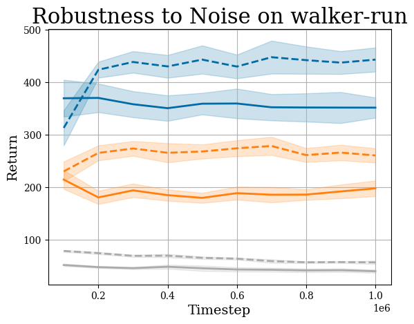
(b)

(c)

Figure 3: Learned Fourier features generalise worse than ReLU features. We apply three different levels of noise to observations at test time—in the medium noise case we find that architectures with learned Fourier feature activations generally perform worse than ReLU only architectures. Results are reported across five seeds. The shaded region represents the standard error of the mean.

4.2 Generalization Properties of Learned Fourier Features

We have shown that periodic activation functions consistently learn high frequency representations. While this improves sample efficiency, it also suggests that learned Fourier feature agents could be overfitting. Following the literature on generalization in RL (Dulac-Arnold et al., 2021), we benchmark generalization by perturbing state observations with Gaussian noise. We only perturb the observations at test time. No training is performed on observations with added noise. As we have shown learned Fourier features and concatenated learned Fourier features learn representations with similar frequencies, we only include the simpler learned Fourier features in our analysis.

Noise levels were tuned by hand for each environment, as the environments have different observation distributions (see appendix 7 for noise scales). We tuned observation noise to 3 different levels per environment: low noise where both ReLU and Fourier features can deploy their policy from training without degradation; medium noise where there is a noticeable impact on performance but the policies learned during training are still useful when compared to an untrained policy (typically with a medium amout of noise there is also a discrepancy in the generalisation performance of Fourier features and ReLU architectures); and lastly high noise, where all policies cannot do better than an untrained agent.

(a)

(b)

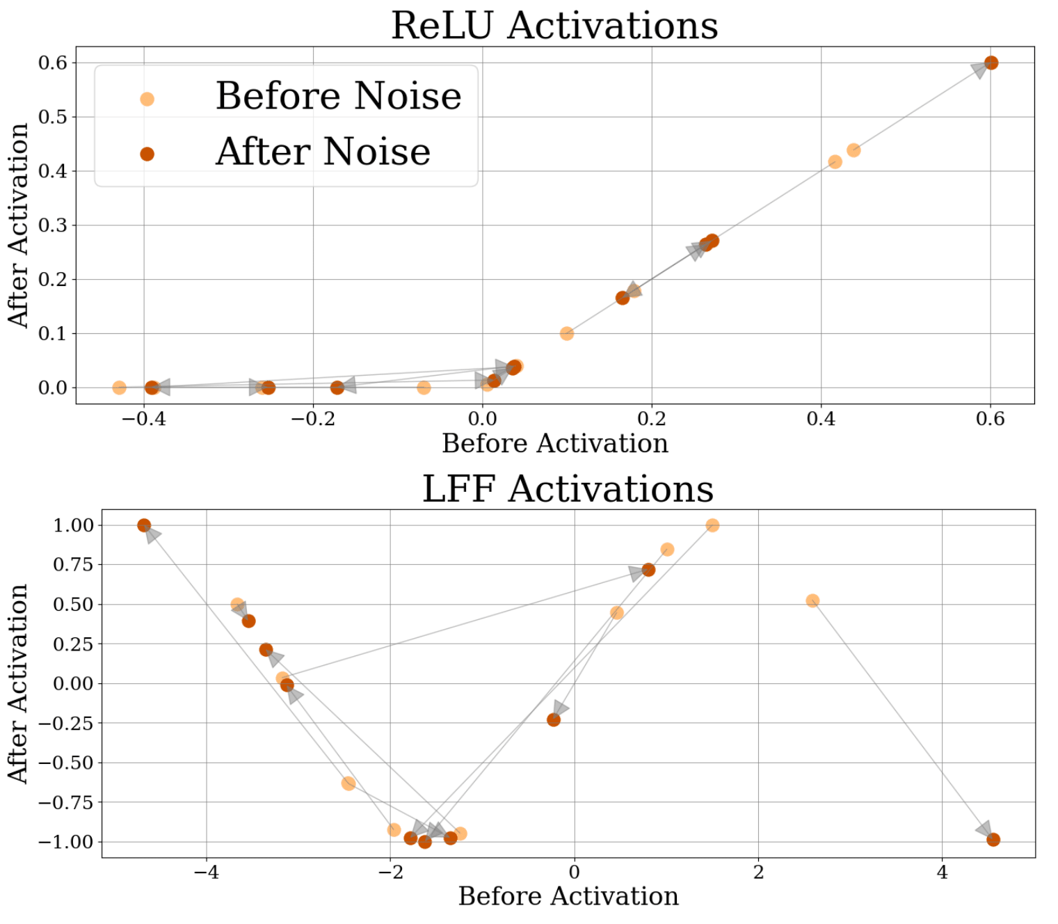
(c)

Figure 4: Periodic activations are more brittle than ReLUs. (a) shows that $\sin$ pre and post-activations become less similar over time more quickly than ReLUs. (b) shows a similar trend in cosine similarity of activations before and after a medium level of noise is applied ($\sigma=0.625$). Qualitatively, LFF activations have their points shifted more dramatically than ReLU activations when inputs are perturbed (panel (c)). Results are reported across five seeds. The shaded regions represent the standard error of the mean.

In the medium noise regime, learned Fourier features are either worse than or comparable to ReLU activation functions at generalizing to noisy observations. Consider the quadruped-run results 3(a), the dotted orange line at 500k steps has a return greater than 500, while the equivalent learned Fourier architecture has a return of approximately 300. This is despite the fact that at 500k timesteps, the performance of ReLU with minimal noise, shown by the dotted blue line, achieves a much higher performance. These results match our intuitions surrounding high frequency representations. They allow value functions to be more expressive and flexible, but with this added flexibility comes the potential for overfitting.

4.3 Why do Fourier Representations Struggle to Generalize?

The relationship between the frequency of learned fourier features and network generalization is perhaps best understood through the lens of feature geometry evolution. Prior work on the expressivity and initialization of neural networks has identified the importance of the effect of a layer on the cosine similarity between the representations of two different inputs prior to and after its application, formalized by the Q/C-maps of Poole et al. (2016). Layers which decorrelate their inputs (i.e. which reduce the cosine similarity) tend to produce networks which are trainable but generalize poorly, while layers which increase the cosine similarity of inputs on average allow the network to generalize more aggressively, potentially at the expense of convergence rates as discussed in greater detail by Martens et al. (2021). Due to their initially low frequency, learned Fourier features begin training with a high cosine similarity before and after activation (see figure 4(b)). However, this value declines as the frequency of the learned fourier features increases over training. The ReLU representations on the other hand see their cosine similarity decrease more slowly than the Fourier features.

A consequence of this phenomenon is that the representation will become more sensitive to perturbations in the input with respect to the Euclidean distance as well. Concretely, we hypothesise that small changes in the input observations will cause larger changes in the post-activation representations than ReLU activations. We find this to be true empirically in table 1, where the Euclidean distance between post activation representations before and after noise is larger for learned Fourier feature representations than for ReLU representations. A qualitative visualisation of this is shown in figure 4(c), where ReLU points are generally correlated before and after noise, while the Fourier representations are more brittle, with dramatic shifts before and after noise.

Table 1: Ratios (learned Fourier features/ReLU) of generalisation properties averaged over all 8 environments (with five seeds each). Uncertainty is standard error of the mean.

Euclidean Distance Ratio	Effective Rank Ratio
3.33 $\pm$ 0.02	7.56 $\pm$ 0.02

Lastly, recent works have quantified the expressivity of neural representations by computing their effective rank—including recent work on classical Fourier features that perform a fixed Fourier decomposition of states Konidaris et al. (2011); Brellmann et al. (2023). Low-rank representations are “implicitly underparameterized” which may help generalization but decrease expressiveness Kumar et al. (2020); Gulcehre et al. (2022). We compute the effective rank of representations from replay buffer samples at the end of training for both ReLU and learned Fourier feature representations in table 1. We report our full results on generalisation in A.5.

4.4 Can the Generalization of Fourier Features be improved?

The previous sections suggest that learned Fourier representations fail to generalize because they learn high frequency representations. Here we introduce a weight decay term in the loss function, which effectively discourages frequencies from growing too large. For both ReLU and periodic activations, we find that a weight decay of 0.1 was optimal. In figure 5, we plot how performance changes over training on the three environments from section 4.2. We find the weight decay has a positive effect on performance for both Fourier representations and ReLU representations. This effect on performance is enough to enable learned Fourier features to be comparable to the performance of the ReLU representations when aggregating results over the three environments (LFF is better on quadruped-run, ReLU is better on walker-run and the two methods are roughly equal in hopper-hop). However, ReLU with weight decay also has improved performance, signalling that there is still a generalization gap to be closed between Fourier representations and ReLU representations.

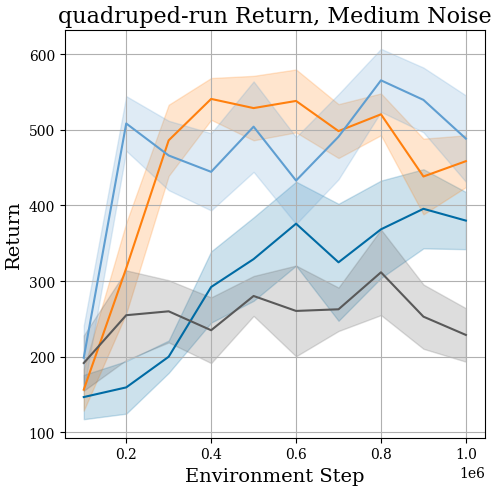
(a)

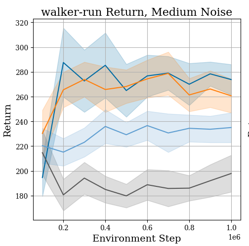
(b)

(c)

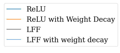
Figure 5: Weight decay is able to partially offset overfitting at a medium level of observation noise, as introduced in section 4.4. In quadruped-run, weight decay allows learned Fourier features generalize as well as a ReLU representations (but not as good as a ReLU representation with weight decay). Results are reported across five seeds. The shaded regions represent the standard error of the mean.

5 Conclusion

We have shown that unconstrained learned Fourier features tend to learn high frequency representations on continuous control tasks. As a result, we hypothesise, and then show empirically, that the high frequency representations do not generalize well. We test generalization by perturbing observation with noise as suggested by (Dulac-Arnold et al., 2021). We provide empirical explanations for why high frequency representations are brittle, showing that small changes in observations leads to large changes in Fourier representations. Lastly, we consider using weight decay as a means to discourage frequency from becoming excessively high—this is able to partially offset the generalization challenges faced by learned Fourier representations.

Appendix A Appendix

A.1 Supervised Learning Warmup

Following previous literature on learned Fourier features Yang et al. (2022), we qualitatively observe the performance of learned Fourier features on the mountain car environment Moore (1990). We first learn a ground truth value function with dynamic programming, using an implementation provided by Yang et al. (2022). Then we try to fit a MLP with ReLU activations and sinusoidal activations to the ground truth value function of the zeroth action, with a checkerboard pattern as the train/test split. We optimise both networks with Adam Kingma & Ba (2014) with a learning rate of $10^{-4}$. Each network has 2 hidden layers of width 400. The learned Fourier feature network has sinusoids throughout to highlight the properties of sinusoidal layers. We use an initial $\beta=10/\pi$. Note this experiment is used to exemplify the potential pitfalls of sinusoidal activations, it has not been tuned to achieve the best possible test error.

A.2 Deepmind Control Hyperparameters

Below we describe in detail the different hyperparameters used by our learned Fourier features agents.

A.2.1 Soft Actor-Critic hyperparameters

Table 2: SAC Haarnoja et al. (2018) hyperparameters that are consistent throughout the baselines.

Hyperparameter	Value
actor learning rate	$10^{-4}$
critic learning rate	$10^{-4}$
temperature learning rate	$10^{-4}$
discount	0.99
target update period	2
initial temperature	0.1
batch size	1024
environment steps before training starts	$10^{4}$

A.2.2 ReLU architecture

Table 3: ReLU Critic architecture

Layer Output Dim	Activation
$20\times(\text{state dimension}+\text{action dimension})$	ReLU
$1024$	ReLU
$1024$	ReLU
$1$	None

Table 4: ReLU Actor architecture

Layer Output Dim	Activation
$1024$	ReLU
$1024$	ReLU
$2\times\text{action dimension}$	output is split into mean and log std dev that parametrizes a Gaussian, tanh is applied to log std dev

A.2.3 Learned Fourier Feature Architecture

Table 5: Learned Fourier feature Critic architecture

Layer Output Dim	Activation
$20\times(\text{state dimension}+\text{action dimension})$	Sinusoid
$1024$	ReLU
$1024$	ReLU
$1$	None

The actor architecture is equivalent to the actor in table 4.

A.2.4 Concatenated Learned Fourier Feature Architecture

Table 6: Concatenated Learned Fourier feature Critic architecture

Layer Output Dim	Activation
$20\times(\text{state dimension}+\text{action dimension})$	Sinusoid, Cosine, None
$1024$	ReLU
$1024$	ReLU
$1$	None

Note the concatenated learned Fourier feature architecture uses a concatenation of a the inputs projected with a sinusoidal activation applied, the inputs projected with a cosine applied and then also just the raw inputs (see equation 4). The actor architecture is again equivalent to the actor in table 4.

A.3 Further Results on Measuring Learned Fourier Frequencies

(a)

(b)

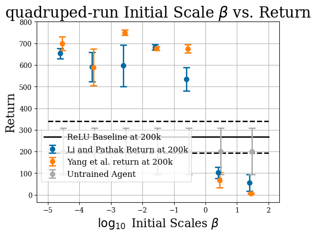
(c)

Figure 6: Full sweep of different intialisations scales $\beta$ vs the return they receive early in training (100k for walker-run, 400k for hopper-hop and 200k for quadruped-run). On walker-run and quadruped-run Fourier features out perform the ReLU and untrained agents baselines.

(a)

(b)

(c)

Figure 7: Scales before and after training for the three different environments considered as well as for a sweep of different $\beta$ initialisations. Provided that $\beta$ is not initialised too high, all learned Fourier feature representations tend to converge to similar frequencies.

(a)

(b)

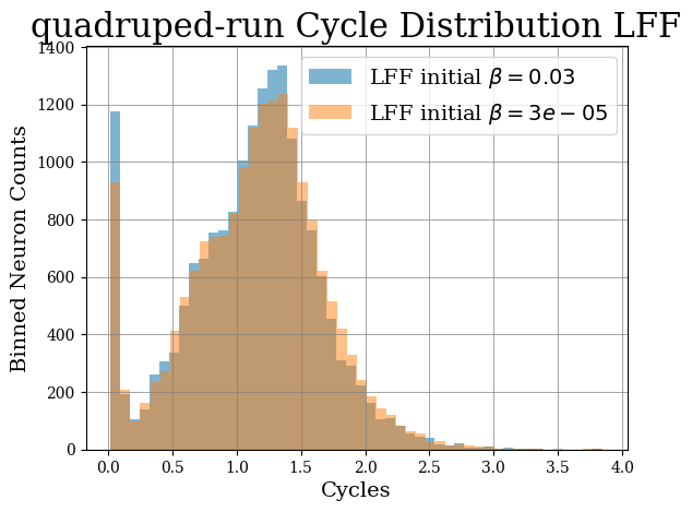
(c)

Figure 8: Neuron frequencies (see definition 3.1 seem to not be influenced by initialisation scale ($\beta$). On all 3 environments, the high $\beta$ and low $\beta$ histograms are mostly overlapping. Furthermore, all representations have a large high frequency component (bins with more than 0.25 cycles).

(a)

(b)

(c)

Figure 9: Cosine similarity before and after a medium level of noise for all three environments.

(a)

(b)

(c)

Figure 10: The cosine similarity before and after activations for the three environments considered.

A.4 Tuning Observation Noise

We tuned observation noise for the different environments to reach low, medium and high levels of disruption on the performance of agents during training. Below is a table of the values of the standard deviation of the isotropic Gaussian noise added to each observations for the different environments.

Table 7: Tuned Levels of Observation Noise for Each Environment

Environment	Noise levels $\sigma$, [low, medium, high]	action size	state size
quadruped-walk	[0.125, 0.625, 1.0]	12	58
cheetah-run	[0.125, 0.625, 1.0]	6	17
acrobot-swingup	[0.05, 0.1, 0.5]	1	6
hopper-hop	[0.125, 0.25, 0.5]	4	15
walker-run	[0.25, 0.375, 1.0]	6	24
finger-turn hard	[0.03, 0.1, 0.15]	2	12
humanoid-run	[0.05, 0.25, 0.5]	21	67
quadruped-run	[0.25, 0.625, 1.0]	12	58

A.5 Full Generalisation Properties results

Table 8: Generalisation properties for all methods averaged over all environments and normalised by the equivalent ReLU quantity.

Method	Effective Rank
ReLU	$1.000\pm 0.002$
ReLU w/ Weight Decay	$0.997\pm 0.001$
LFF	$7.558\pm 0.021$
LFF w/ Weight Decay	$5.242\pm 0.017$

Table 9: Average effective rank over all environments, normalised by the rank for a ReLU network on each environment.

Method	Averaged Euclidean Distance
ReLU	$1.000\pm 0.006$
ReLU w/ Weight Decay	$0.266\pm 0.002$
LFF	$3.329\pm 0.020$
LFF w/ Weight Decay	$2.099\pm 0.014$

Table 10: Average Euclidean distance before and after noise of the different representations considered for a medium level of noise, normalised by the Euclidean distance for a ReLU network.

A.5.1 Full Deepmind Control Results

We plot the generalisation results for all environments for low, medium and high levels of noise (as described in table 7).

A.5.2 Low Noise Observation Pertubations

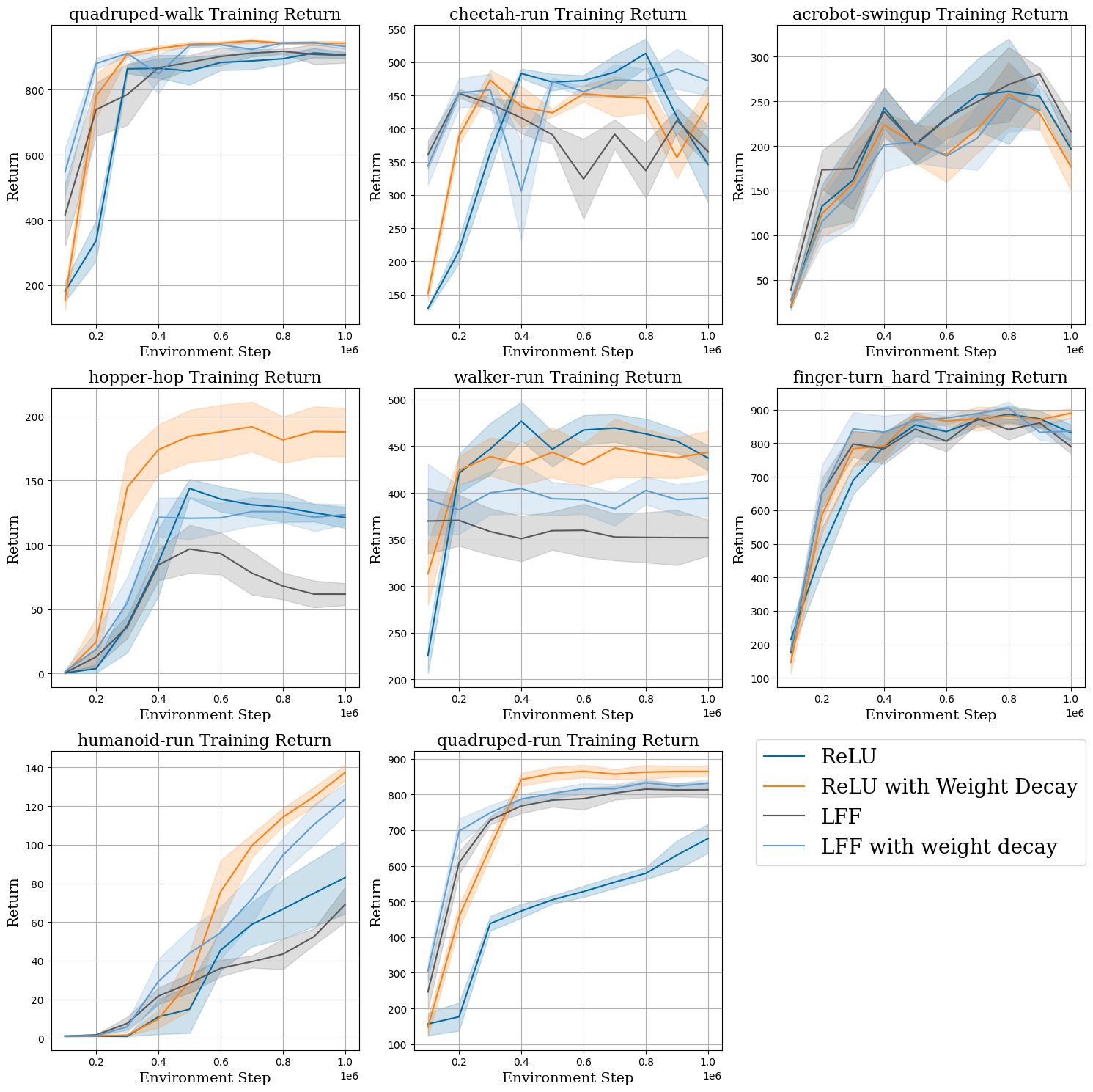
Figure 11: Full evaluating curves for all 8 environments plotted for a low amount of noise (see table 7). Here the benefits of ReLU activations over LFF representations are still present in one environment (quadruped-walk), however even with this low level of noise ReLU activations begin to outperform or match Fourier feature representations.

A.5.3 Medium Noise Observation Pertubations

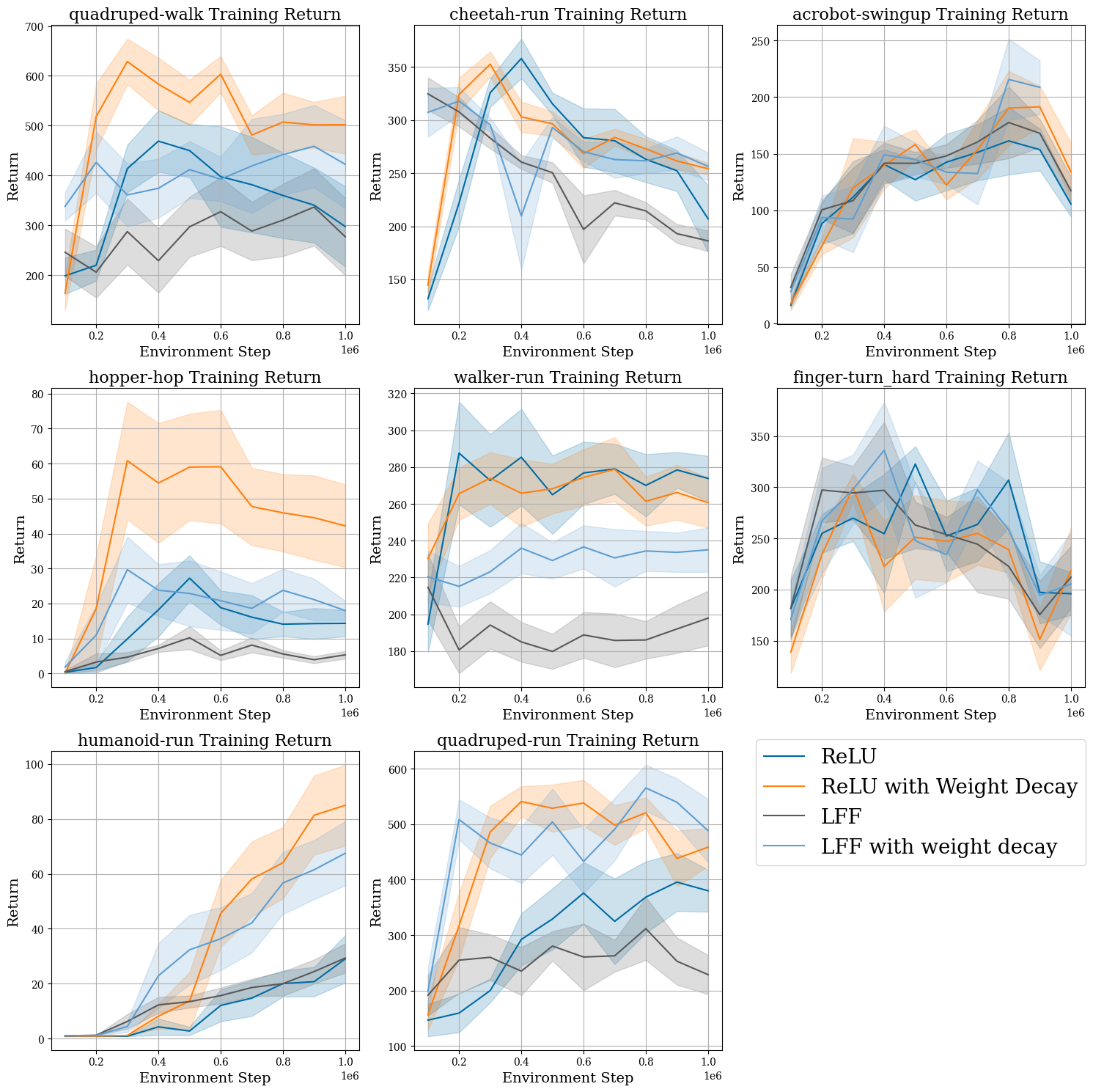
Figure 12: In the medium noise setting (see table 7) the learned Fourier features network performs worse on 4/8 environments than ReLU networks (cheetah-run, hopper-hop, walker-run, quadruped-walk and quadruped-run).

A.5.4 High Noise Observation Pertubations

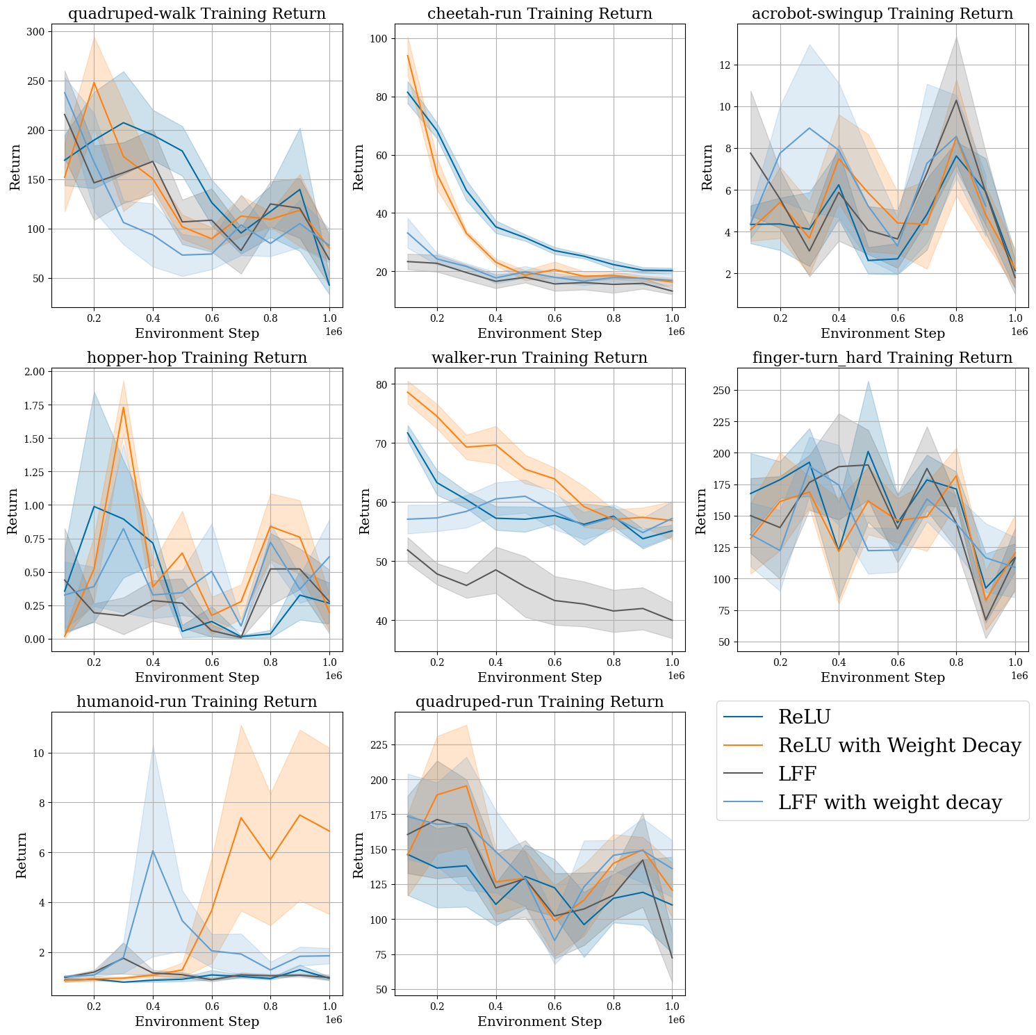
Figure 13: In the high noise regime, all algorithms exhibit poor performance on all 8 environments.

References

- Achiam et al. (2019) Joshua Achiam, Ethan Knight, and Pieter Abbeel. Towards characterizing divergence in deep q-learning. arXiv preprint arXiv:1903.08894, 2019.
- Badia et al. (2020) Adrià Puigdomènech Badia, Bilal Piot, Steven Kapturowski, Pablo Sprechmann, Alex Vitvitskyi, Zhaohan Daniel Guo, and Charles Blundell. Agent57: Outperforming the atari human benchmark. In International conference on machine learning, pp. 507–517. PMLR, 2020.
- Barry et al. (2007) Caswell Barry, Robin Hayman, Neil Burgess, and Kathryn J Jeffery. Experience-dependent rescaling of entorhinal grids. Nature neuroscience, 10(6):682–684, 2007.
- Bengio et al. (2021) Emmanuel Bengio, Joelle Pineau, and Doina Precup. Correcting momentum in temporal difference learning. arXiv preprint arXiv:2106.03955, 2021.
- Bradbury et al. (2018) James Bradbury, Roy Frostig, Peter Hawkins, Matthew James Johnson, Chris Leary, Dougal Maclaurin, George Necula, Adam Paszke, Jake VanderPlas, Skye Wanderman-Milne, and Qiao Zhang. JAX: composable transformations of Python+NumPy programs, 2018. URL http://github.com/google/jax.
- Brellmann et al. (2023) David Brellmann, David Filliat, and Goran Frehse. Fourier features in reinforcement learning with neural networks. Transactions on Machine Learning Research Journal, 2023.
- Cobb et al. (2020) Oliver J Cobb, Christopher GR Wallis, Augustine N Mavor-Parker, Augustin Marignier, Matthew A Price, Mayeul d’Avezac, and Jason D McEwen. Efficient generalized spherical cnns. arXiv preprint arXiv:2010.11661, 2020.
- Cobbe et al. (2019) Karl Cobbe, Oleg Klimov, Chris Hesse, Taehoon Kim, and John Schulman. Quantifying generalization in reinforcement learning. In International Conference on Machine Learning, pp. 1282–1289. PMLR, 2019.
- Cohen et al. (2018) Taco S Cohen, Mario Geiger, Jonas Köhler, and Max Welling. Spherical cnns. arXiv preprint arXiv:1801.10130, 2018.
- Dayan (1993) Peter Dayan. Improving generalization for temporal difference learning: The successor representation. Neural computation, 5(4):613–624, 1993.
- Dohare et al. (2023) Shibhansh Dohare, Juan Hernandez-Garcia, Parash Rahman, Richard Sutton, and A Rupam Mahmood. Loss of plasticity in deep continual learning. 2023.
- Dulac-Arnold et al. (2021) Gabriel Dulac-Arnold, Nir Levine, Daniel J Mankowitz, Jerry Li, Cosmin Paduraru, Sven Gowal, and Todd Hester. Challenges of real-world reinforcement learning: definitions, benchmarks and analysis. Machine Learning, 110(9):2419–2468, 2021.
- Ghiassian et al. (2020) Sina Ghiassian, Banafsheh Rafiee, Yat Long Lo, and Adam White. Improving performance in reinforcement learning by breaking generalization in neural networks. arXiv preprint arXiv:2003.07417, 2020.
- Gulcehre et al. (2022) Caglar Gulcehre, Srivatsan Srinivasan, Jakub Sygnowski, Georg Ostrovski, Mehrdad Farajtabar, Matt Hoffman, Razvan Pascanu, and Arnaud Doucet. An empirical study of implicit regularization in deep offline rl. arXiv preprint arXiv:2207.02099, 2022.
- Haarnoja et al. (2018) Tuomas Haarnoja, Aurick Zhou, Pieter Abbeel, and Sergey Levine. Soft actor-critic: Off-policy maximum entropy deep reinforcement learning with a stochastic actor. In International conference on machine learning, pp. 1861–1870. PMLR, 2018.
- Jacot et al. (2018) Arthur Jacot, Franck Gabriel, and Clément Hongler. Neural tangent kernel: Convergence and generalization in neural networks. Advances in neural information processing systems, 31, 2018.
- Kingma & Ba (2014) Diederik P Kingma and Jimmy Ba. Adam: A method for stochastic optimization. arXiv preprint arXiv:1412.6980, 2014.
- Kirk et al. (2023) Robert Kirk, Amy Zhang, Edward Grefenstette, and Tim Rocktäschel. A survey of zero-shot generalisation in deep reinforcement learning. Journal of Artificial Intelligence Research, 76:201–264, 2023.
- Konidaris et al. (2011) George Konidaris, Sarah Osentoski, and Philip Thomas. Value function approximation in reinforcement learning using the fourier basis. In Proceedings of the AAAI Conference on Artificial Intelligence, volume 25, pp. 380–385, 2011.
- Kostrikov (2021) Ilya Kostrikov. JAXRL: Implementations of Reinforcement Learning algorithms in JAX, 10 2021. URL https://github.com/ikostrikov/jaxrl.
- Krizhevsky et al. (2012) Alex Krizhevsky, Ilya Sutskever, and Geoffrey E Hinton. Imagenet classification with deep convolutional neural networks. Advances in neural information processing systems, 25, 2012.
- Kulkarni et al. (2016) Tejas D Kulkarni, Ardavan Saeedi, Simanta Gautam, and Samuel J Gershman. Deep successor reinforcement learning. arXiv preprint arXiv:1606.02396, 2016.
- Kumar et al. (2020) Aviral Kumar, Rishabh Agarwal, Dibya Ghosh, and Sergey Levine. Implicit under-parameterization inhibits data-efficient deep reinforcement learning. arXiv preprint arXiv:2010.14498, 2020.
- Li & Pathak (2021) Alexander Li and Deepak Pathak. Functional regularization for reinforcement learning via learned fourier features. Advances in Neural Information Processing Systems, 34:19046–19055, 2021.
- Li et al. (2020) Zongyi Li, Nikola Kovachki, Kamyar Azizzadenesheli, Burigede Liu, Kaushik Bhattacharya, Andrew Stuart, and Anima Anandkumar. Fourier neural operator for parametric partial differential equations. arXiv preprint arXiv:2010.08895, 2020.
- Lyle et al. (2022) Clare Lyle, Mark Rowland, Will Dabney, Marta Kwiatkowska, and Yarin Gal. Learning dynamics and generalization in deep reinforcement learning. In International Conference on Machine Learning, pp. 14560–14581. PMLR, 2022.
- Martens et al. (2021) James Martens, Andy Ballard, Guillaume Desjardins, Grzegorz Swirszcz, Valentin Dalibard, Jascha Sohl-Dickstein, and Samuel S Schoenholz. Rapid training of deep neural networks without skip connections or normalization layers using deep kernel shaping. arXiv preprint arXiv:2110.01765, 2021.
- McCaughan (1997) D.B. McCaughan. On the properties of periodic perceptrons. In Proceedings of International Conference on Neural Networks (ICNN’97), volume 1, pp. 188–193 vol.1, 1997. doi: 10.1109/ICNN.1997.611662.
- Mildenhall et al. (2021) Ben Mildenhall, Pratul P Srinivasan, Matthew Tancik, Jonathan T Barron, Ravi Ramamoorthi, and Ren Ng. Nerf: Representing scenes as neural radiance fields for view synthesis. Communications of the ACM, 65(1):99–106, 2021.
- Moore (1990) Andrew William Moore. Efficient memory-based learning for robot control. Technical report, University of Cambridge, Computer Laboratory, 1990.
- Nanda et al. (2023) Neel Nanda, Lawrence Chan, Tom Lieberum, Jess Smith, and Jacob Steinhardt. Progress measures for grokking via mechanistic interpretability. arXiv preprint arXiv:2301.05217, 2023.
- Nikishin et al. (2022) Evgenii Nikishin, Max Schwarzer, Pierluca D’Oro, Pierre-Luc Bacon, and Aaron Courville. The primacy bias in deep reinforcement learning. In International conference on machine learning, pp. 16828–16847. PMLR, 2022.
- Poole et al. (2016) Ben Poole, Subhaneil Lahiri, Maithra Raghu, Jascha Sohl-Dickstein, and Surya Ganguli. Exponential expressivity in deep neural networks through transient chaos. Advances in neural information processing systems, 29, 2016.
- Rahaman et al. (2019) Nasim Rahaman, Aristide Baratin, Devansh Arpit, Felix Draxler, Min Lin, Fred Hamprecht, Yoshua Bengio, and Aaron Courville. On the spectral bias of neural networks. In Kamalika Chaudhuri and Ruslan Salakhutdinov (eds.), Proceedings of the 36th International Conference on Machine Learning, volume 97 of Proceedings of Machine Learning Research, pp. 5301–5310. PMLR, 09–15 Jun 2019. URL https://proceedings.mlr.press/v97/rahaman19a.html.
- Rahimi & Recht (2007) Ali Rahimi and Benjamin Recht. Random features for large-scale kernel machines. Advances in neural information processing systems, 20, 2007.
- Salimans & Kingma (2016) Tim Salimans and Durk P Kingma. Weight normalization: A simple reparameterization to accelerate training of deep neural networks. Advances in neural information processing systems, 29, 2016.
- Sherstov & Stone (2005) Alexander A Sherstov and Peter Stone. Function approximation via tile coding: Automating parameter choice. In International symposium on abstraction, reformulation, and approximation, pp. 194–205. Springer, 2005.
- Silver et al. (2013) David Silver, Alex Graves Ioannis Antonoglou Daan Wierstra, and Martin Riedmiller. Playing atari with deep reinforcement learning. DeepMind Lab. arXiv, 1312, 2013.
- Silver et al. (2016) David Silver, Aja Huang, Chris J Maddison, Arthur Guez, Laurent Sifre, George Van Den Driessche, Julian Schrittwieser, Ioannis Antonoglou, Veda Panneershelvam, Marc Lanctot, et al. Mastering the game of go with deep neural networks and tree search. nature, 529(7587):484–489, 2016.
- Sitzmann et al. (2020) Vincent Sitzmann, Julien Martel, Alexander Bergman, David Lindell, and Gordon Wetzstein. Implicit neural representations with periodic activation functions. In H. Larochelle, M. Ranzato, R. Hadsell, M.F. Balcan, and H. Lin (eds.), Advances in Neural Information Processing Systems, volume 33, pp. 7462–7473. Curran Associates, Inc., 2020. URL https://proceedings.neurips.cc/paper_files/paper/2020/file/53c04118df112c13a8c34b38343b9c10-Paper.pdf.
- Sutton & Barto (2018) Richard S Sutton and Andrew G Barto. Reinforcement learning: An introduction. MIT press, 2018.
- Tancik et al. (2020) Matthew Tancik, Pratul Srinivasan, Ben Mildenhall, Sara Fridovich-Keil, Nithin Raghavan, Utkarsh Singhal, Ravi Ramamoorthi, Jonathan Barron, and Ren Ng. Fourier features let networks learn high frequency functions in low dimensional domains. Advances in Neural Information Processing Systems, 33:7537–7547, 2020.
- Tassa et al. (2018) Yuval Tassa, Yotam Doron, Alistair Muldal, Tom Erez, Yazhe Li, Diego de Las Casas, David Budden, Abbas Abdolmaleki, Josh Merel, Andrew Lefrancq, et al. Deepmind control suite. arXiv preprint arXiv:1801.00690, 2018.
- van Hasselt et al. (2018) Hado van Hasselt, Yotam Doron, Florian Strub, Matteo Hessel, Nicolas Sonnerat, and Joseph Modayil. Deep reinforcement learning and the deadly triad. arXiv preprint arXiv:1812.02648, 2018.
- Whiteson (2010) Shimon Whiteson. Adaptive tile coding. Adaptive Representations for Reinforcement Learning, pp. 65–76, 2010.
- Yang et al. (2022) Ge Yang, Anurag Ajay, and Pulkit Agrawal. Overcoming the spectral bias of neural value approximation. arXiv preprint arXiv:2206.04672, 2022.
- Yu et al. (2020) Changmin Yu, Timothy EJ Behrens, and Neil Burgess. Prediction and generalisation over directed actions by grid cells. arXiv preprint arXiv:2006.03355, 2020.