Periodic agent-state based Q-learning for POMDPs

Abstract

The standard approach for Partially Observable Markov Decision Processes (POMDPs) is to convert them to a fully observed belief-state MDP. However, the belief state depends on the system model and is therefore not viable in reinforcement learning (RL) settings. A widely used alternative is to use an agent state, which is a model-free, recursively updateable function of the observation history. Examples include frame stacking and recurrent neural networks. Since the agent state is model-free, it is used to adapt standard RL algorithms to POMDPs. However, standard RL algorithms like Q-learning learn a stationary policy. Our main thesis that we illustrate via examples is that because the agent state does not satisfy the Markov property, non-stationary agent-state based policies can outperform stationary ones. To leverage this feature, we propose PASQL (periodic agent-state based Q-learning), which is a variant of agent-state-based Q-learning that learns periodic policies. By combining ideas from periodic Markov chains and stochastic approximation, we rigorously establish that PASQL converges to a cyclic limit and characterize the approximation error of the converged periodic policy. Finally, we present a numerical experiment to highlight the salient features of PASQL and demonstrate the benefit of learning periodic policies over stationary policies.

1 Introduction

Recent advances in reinforcement learning (RL) have successfully integrated algorithms with strong theoretical guarantees and deep learning to achieve significant successes [Mni+13, Sil+16]. However, most RL theory is limited to models with perfect state observations [SB08, BT96]. Despite this, there is substantial empirical evidence showing that RL algorithms perform well in partially observed settings [Wie+07, Wie+10, Hau00, HS15, Gru+18, Kap+19, Haf+20, Haf+21]. Recently, there has been a significant advances in the theoretical understanding of different RL algorithms for POMDPs [Sub+22, KY22, Sey+23, DRZ22] but a complete understanding is still lacking.

Planning in POMDPs. When the system model is known, the standard approach [Åst65, SS73, CKL94] is to construct an equivalent MDP with the belief state (which is the posterior distribution of the environment state given the history of observations and actions at the agent) as the information state. The belief state is policy independent and has time-homogeneous dynamics, which enables the formulation of a belief-state based dynamic program (DP). There is a rich literature which leverages the structure of the resulting DP to propose efficient algorithms to solve POMDPs [SS73, CKL94, CLZ97, Cha07, Zha09, PGT+03, SS04, SV05]. See [KWW22] for a review. However, the belief state depends on the system model, so the belief-state based approach does not work for RL.

RL in POMDPs. An alternative approach for RL in POMDPs is to consider policies which depend on an agent state $\{z_{t}\}_{t\geq 1}$, where $Z_{t}\in\mathsf{Z}$, which is a recursively updateable compression of the history: the agent starts at an initial state $z_{0}$ and recursively updates the agent state as some function of the current agent-state, next observation, and current action. A simple instance of agent-state is frame stacking, where a window of previous observations is used as state [WS94, Mni+13, KY22]. Another example is to use a recurrent neural network such as LSTM or GRU to compress the history of observations and actions into an agent state [Wie+07, Wie+10, HS15, Kap+19, Haf+20]. In fact, as argued in [DVZ22, Lu+23] such an agent state is present in most deep RL algorithms for POMDPs. We refer to such a representation as an “agent state” because it captures the agent’s internal state that it uses for decision making.

When the agent state satisfies the Markov property, i.e., $\mathds{P}(z_{t+1}\mid z_{1:t},a_{1:t})=\mathds{P}(z_{t+1}\mid z_{t},a_{t})$, where $a_{t}$ is the action, the optimal agent-state based policy can be obtained via a dynamic program (DP) [Sub+22]. An example of such an agent state is the belief state. However, the Markov property is not always satisfied, for example, it need not be satisfied when using frame stacking. In such settings, the best agent-state policy cannot be obtained via a DP. Nonetheless, there has been considerable interest to use RL to find a good agent-state based policy. One of the most commonly used RL algorithms is off-policy Q-learning, which we call agent-state Q-learning (ASQL). In ASQL for POMDPs, the Q-learning iteration is applied as if the agent state satisfied the Markov property even though it does not. The agent starts with an initial $Q_{1}(z,a)$, acts according to a behavior policy $\mu$, i.e., chooses $a_{t}\sim\mu(z_{t})$, and recursively updates

$$Q_{t+1}(z,a)=Q_{t}(z,a)+\alpha_{t}(z,a)\Bigl{[}R_{t}+\gamma\max_{a^{\prime}\in\mathsf{A}}Q_{t}(z_{t+1},a^{\prime})-Q_{t}(z,a)\Bigr{]}$$ (ASQL)

where $R_{t}$ is the reward at time $t$ and the learning rates $\{\alpha_{t}\}_{t\geq 1}$ is chosen such that $\alpha_{t}(z,a)=0$ if $(z,a)\neq(z_{t},a_{t})$. The convergence of ASQL has been recently presented in [KY22, Sey+23] which show that under some technical assumptions, ASQL converges to a limit. The policy determined by ASQL is the greedy policy w.r.t. this limit.

Limitation of Q-learning with agent state. The greedy policy determined by ASQL is stationary (i.e., uses the same control law at every time). In infinite horizon MDPs (and, therefore, also in POMDPs when using the belief state as an agent state), stationary policies perform as well as non-stationary policies. This is because the agent-state satisfies the Markov property. However, in ASQL the agent state generally does not satisfy the Markov property. Therefore, restricting attention to stationary policies may lead to a loss of optimality!

Figure 1: The cells indicate the state of the environment. Cells with the same background color have the same observation. The cells with a thick red boundary correspond to elements of the set $\mathsf{D}_{0}\coloneqq\{n(n+1)/2+1:n\in\mathds{N}\}$, where the action $0$ gives a reward of $+1$ and moves the state to the right, while the action $1$ gives a reward of $-1$ and resets the state to $1$. The cells with a thin black boundary correspond to elements of the set $\mathsf{D}_{1}=\mathds{N}\setminus\mathsf{D}_{0}$, where the action $1$ gives the reward of $+1$ and moves the state to the right while the action $0$ gives a reward of $-1$ and resets the state to $1$. Discount factor $\gamma=0.9$.

As an illustration, consider the POMDP shown in Fig. 1, which is described in detail in App. A.2 as Ex. 2. Suppose the system starts in state $1$. Since the dynamics are deterministic, the agent can infer the current state from the history of past actions and can take the action to increment the current state and receive a per-step reward of $+1$. Thus, the performance $J^{\star}_{\textsc{{bd}}}$ of belief-state based policies is $J^{\star}_{\textsc{{bd}}}=1/(1-\gamma)$. Contrast this with the performance $J^{\star}_{\textsc{{sd}}}$ of deterministic agent-state base policies with agent state equal to current observation, which is given by $J^{\star}_{\textsc{{sd}}}=(1+\gamma-\gamma^{2})/(1-\gamma^{3})<J^{\star}_{\textsc{{bd}}}$.

We show that the gap between $J^{\star}_{\textsc{{sd}}}$ and $J^{\star}_{\textsc{{bd}}}$ can be reduced by considering non-stationary policies. Ex. 2 has deterministic dynamics, so the optimal policy can be implemented in open-loop via a sequence of control actions $\{a^{\star}_{t}\}_{t\geq 1}$, where $a^{\star}_{t}=\mathds{1}\{t\in\mathsf{D}_{1}\}$. This open-loop policy can be implemented via any information structure, including agent-state based policies. Thus, a non-stationary deterministic agent-state based policy performs better than stationary deterministic agent-state based policies. A similar conclusion also holds for models with stochastic dynamics.

The main idea. Arbitrary non-stationary policies cannot be used in RL because such policies have countably infinite number of parameters. In this paper, we consider a simple class of non-stationary policies with finite number of parameters: periodic policies. An agent-state based policy $\pi=(\pi_{1},\pi_{2},\dots)$ is said to be periodic with period $L$ if $\pi_{t}=\pi_{t^{\prime}}$ whenever $t\equiv t^{\prime}\pmod{L}$.

To highlight the salient feature of periodic policies, we perform a brute force search over all deterministic periodic policies of period $L$, for $L=\{1,\dots,10\}$, in Ex. 2. Let $J^{\star}_{L}$ denote the optimal performance for policies of period $L$. The result is shown below (see App. A.2 for details):

$$L$$ 1 2 3 4 5 6 7 8 9 10

4.022 4.022 7.479 6.184 8.810 7.479 9.340 8.488 9.607 8.810

The above example highlights some salient features of periodic policies: (i) Periodic deterministic agent-state based policies may outperform stationary deterministic agent-state based policies. (ii) $\{J^{\star}_{L}\}_{L\geq 1}$is not a monotonically increasing sequence. This is because $\Pi_{L}$, the set of all periodic deterministic agent-state based policies of period $L$, is not monotonically increasing. (iii) If $L$ divides $M$, then $J^{\star}_{L}\leq J^{\star}_{M}$. This is because $\Pi_{L}\subseteq\Pi_{M}$. Therefore, periodic policies with period $L\in\{n!:n\in\mathds{N}\}$ will have monotonically increasing performance. (iv) In the above example, the set $\mathsf{D}_{0}$ is chosen such that the optimal sequence of actions is not periodic. Therefore, even though periodic policies can achieve a performance that is arbitrarily close to the optimal belief-based policies, they are not necessarily globally optimal (in the class of non-stationary agent-state based policies). Thus, the periodic deterministic policy class is a middle ground between the stationary deterministic and non-stationary policy classes and provides us a simple way of leveraging the benefits of non-stationarity while trading-off computational and memory complexity.

The main contributions of this paper are as follows.

1. Motivated by the fact that non-stationary agent-state based policies outperform stationary ones, we propose a variant of agent-state based Q-learning (ASQL) that learns periodic policies. We call this algorithm periodic agent-state based Q-learning (PASQL).

2. We rigorously establish that PASQL converges to a cyclic limit. Therefore, the greedy policy w.r.t. the limit is a periodic policy. Due to the non-Markovian nature of the agent-state, the limit (of the Q-function and the greedy policy) depends on the behavioral policy used during learning.

3. We quantify the sub-optimality gap of the periodic policy learnt by PASQL.

4. We present numerical experiments to illustrate the convergence results, highlight the salient features of PASQL, and show that the periodic policy learned by PASQL indeed performs better than stationary policies learned by ASQL.

2 Periodic agent-state based Q-learning (PASQL) with agent state

2.1 Model for POMDPs

A POMDP is a stochastic dynamical system with state $s_{t}\in\mathsf{S}$, input $a_{t}\in\mathsf{A}$, and output $y_{t}\in\mathsf{Y}$, where we assume that all sets are finite. The system operates in discrete time with the dynamics given as follows: The initial state $s_{1}\sim\rho$ and for any time $t\in\mathds{N}$, we have

$$\mathds{P}(s_{t+1},y_{t+1}\mid s_{1:t},y_{1:t},a_{1:t})=\mathds{P}(s_{t+1},y_{t+1}\mid s_{t},a_{t})\eqqcolon P(s_{t+1},y_{t+1}\mid s_{t},a_{t})$$ (1)

where $P$ is a probability transition matrix. In addition, at each time the system yields a reward $R_{t}=r(s_{t},a_{t})$. We will assume that $R_{t}\in[0,R_{\max}]$. The discount factor is denoted by $\gamma\in[0,1)$.

Let $\vec{\pi}=(\vec{\pi}_{1},\vec{\pi}_{2},\dots)$ denote any (history dependent and possibly randomized) policy. Then the action at time $t$ is given by $a_{t}\sim\vec{\pi}_{t}(y_{1:t},a_{1:t-1})$. The performance of policy $\vec{{\pi}}$ is given by

$$J^{\vec{{\pi}}}\coloneqq\mathds{E}_{\begin{subarray}{c}a_{t}\sim\vec{\pi}_{t}(y_{1:t},a_{t-1})\\ (s_{t+1},y_{t+1})\sim P(s_{t},a_{t})\end{subarray}}\biggl{[}\medop\sum_{t=1}^{\infty}\gamma^{t-1}r(s_{t},a_{t})\biggm{|}s_{1}\sim\rho\biggr{]}.$$ (2)

The objective is to find a (history dependent and possibly randomized) policy $\vec{{\pi}}$ to maximize $J^{\vec{{\pi}}}$.

Agent state for POMDPs. An agent-state is model-free recursively updateable function of the history of observations and actions. In particular, let $\mathsf{Z}$ denote agent-state space. Then, the agent state process $\{z_{t}\}_{t\geq 0}$, $z_{t}\in\mathsf{Z}$, starts with an initial value $z_{0}$, and is then recursively computed as $z_{t+1}=\phi(z_{t},y_{t+1},a_{t})$ for a pre-specified agent-state update function $\phi$.

We use ${\pi}=(\pi_{1},\pi_{2},\dots)$ to denote an agent-state based policy, i.e., a policy where the action at time $t$ is given by $a_{t}\sim\pi_{t}(z_{t})$. An agent-state based policy is said to be stationary if for all $t$ and $t^{\prime}$, we have $\pi_{t}(a|z)=\pi_{t^{\prime}}(a|z)$ for all $(z,a)\in\mathsf{Z}\times\mathsf{A}$. An agent-state based policy is said to be periodic with period $L$ if for all $t$ and $t^{\prime}$ such that $t\equiv t^{\prime}\pmod{L}$, we have $\pi_{t}(a|z)=\pi_{t^{\prime}}(a|z)$ for all $(z,a)\in\mathsf{Z}\times\mathsf{A}$.

2.2 PASQL: Periodic agent-state based Q-learning algorithm for POMDPs

We now present a periodic variant of agent-state based Q-learning, which we abbreviate as PASQL. PASQL is an online, off-policy learning algorithm in which the agent acts according to a behavior policy $\mu=(\mu_{1},\mu_{2},\dots)$ which is a periodic (stochastic) agent-state based policy $\mu$ with period $L$.

Let $\llbracket t\rrbracket\coloneqq(t\bmod L)$ and $\mathsf{L}\coloneqq\{0,1,\dots,L-1\}$. Let $(z_{1},a_{1},R_{1},z_{2},a_{2},R_{2},\dots)$ be a sample path of agent-state, action, and reward observed by the agent. In PASQL, the agent maintains an $L$-tuple of Q-functions $(Q^{0}_{t},Q^{1}_{t},\dots,Q^{L-1}_{t})$, $t\geq 1$. The $\ell$-th component, $\ell\in\mathsf{L}$, is updated at time steps when $\llbracket t\rrbracket=\ell$. In particular, we can write the update as

$$Q^{\ell}_{t+1}(z,a)=Q^{\ell}_{t}(z,a)+\alpha^{\ell}_{t}(z,a)\Bigl{[}R_{t}+\gamma\max_{a^{\prime}\in\mathsf{A}}Q^{\llbracket\ell+1\rrbracket}_{t}(z_{t+1},a^{\prime})-Q^{\ell}_{t}(z,a)\Bigr{]},\quad\forall\ell\in\mathsf{L},$$ (PASQL)

where the learning rate sequence $\{(\alpha^{0}_{t},\dots,\alpha^{L-1}_{t})\}_{t\geq 1}$ has the property that $\alpha^{\ell}_{t}(z,a)=0$ if $(\ell,z,a)\neq(\llbracket t\rrbracket,z_{t},a_{t})$. PASQL differs from ASQL in two aspects: (i) The behavior policy $\mu$ is periodic. (ii) The update of the Q-function is periodic. When $L=1$, PASQL collapses to ASQL.

The standard convergence analysis of Q-learning for MDPs shows that the Q-function convergences to the unique solution of the MDP dynamic program (DP). The key challenge in characterizing the convergence of PASQL is that the agent state $\{Z_{t}\}_{t\geq 1}$ does not satisfy the Markov property. Therefore, a DP to find the best agent-state based policy does not exist. So, we cannot use the standard analysis to characterize the convergence of PASQL. In Sec. 2.3, we provide a complete characterization of the convergence of PASQL.

The quality of the converged solution depends on the expressiveness of the agent state. For example, if the agent state is not expressive (e.g., agent state is always constant), then even if PASQL converges to a limit, the limit will be far from optimal. Therefore, it is important to quantify the degree of sub-optimality of the converged limit. We do so in Sec. 2.4.

2.3 Establishing the convergence of tabular PASQL

To characterize the convergence of tabular PASQL, we impose two assumptions which are standard for analysis of RL algorithms [JSJ94, BT96]. The first assumption is on the learning rates.

Assumption 1

For all $(\ell,z,a)$, we have $\sum_{t\geq 1}\alpha^{\ell}_{t}(z,a)=\infty$ and $\sum_{t\geq 1}(\alpha^{\ell}_{t}(z,a))^{2}<\infty$.

The second assumption is on the behavior policy $\mu$. We first state an immediate property.

Lemma 1

For any behavior policy $\mu$, the process $\{(S_{t},Y_{t},Z_{t},A_{t})\}_{t\geq 1}$ is a Markov chain. _□

Assumption 2

The behavior policy $\mu$ is such that the Markov chain $\{(S_{t},Y_{t},Z_{t},A_{t})\}_{t\geq 1}$ is time-periodic with period $L$ and converges to a cyclic limiting distribution $(\zeta_{\mu}^{0},\dots,\zeta_{\mu}^{L-1})$, where $\sum_{(s,y)}\zeta_{\mu}^{\ell}(s,y,z,a)>0$ for all $(\ell,z,a)$ (i.e., all $(\ell,z,a)$ are visited infinitely often).

For the ease of notation, we will continue to use $\zeta_{\mu}^{\ell}$ to denote the marginal and conditional distributions w.r.t. $\zeta_{\mu}^{\ell}$. In particular, for marginals we use $\zeta_{\mu}^{\ell}(y,z,a)$ to denote $\sum_{s\in\mathsf{S}}\zeta_{\mu}^{\ell}(s,y,z,a)$ and so on; for conditionals, we use $\zeta_{\mu}^{\ell}(s|z,a)$ to denote $\zeta_{\mu}^{\ell}(s,z,a)/\zeta_{\mu}^{\ell}(z,a)$ and so on.

Theorem 1

Under Assms. 1 and 2, the process $\{(Q^{0}_{t},\dots,Q^{L-1}_{t})\}_{t\geq 1}$ converges to a limit $(Q^{0}_{\mu},\dots,Q^{L-1}_{\mu})$ a.s., where the limit is the unique fixed point of the DP for a periodic MDP:

$$Q^{\ell}_{\mu}(z,a)=r^{\ell}_{\mu}(z,a)+\gamma\medop\sum_{z^{\prime}\in\mathsf{Z}}P^{\ell}_{\mu}(z^{\prime}|z,a)\max_{a^{\prime}\in\mathsf{A}}Q^{\llbracket\ell+1\rrbracket}_{\mu}(z^{\prime},a^{\prime}),\quad\forall\ell\in\mathsf{L},\forall(z,a)\in\mathsf{Z}\times\mathsf{A}$$ (3)

where the periodic rewards $(r^{0}_{\mu},\dots,r^{L-1}_{\mu})$ and dynamics $(P^{0}_{\mu},\dots,P^{L-1}_{\mu})$ are given by

$$r^{\ell}_{\mu}(z,a) \coloneqq\medop\sum_{s\in\mathsf{S}}r(s,a)\zeta_{\mu}^{\ell}(s,z,a), P^{\ell}_{\mu}(z^{\prime}|z,a) \coloneqq\smashoperator[]{\medop\sum_{(s,y^{\prime})\in\mathsf{S}\times\mathsf{Y}}^{}}\mathds{1}_{\{z^{\prime}=\phi(z,y^{\prime},a)\}}P(y^{\prime}|s,a)\zeta_{\mu}^{\ell}(s|z,a).$$ (4)

_□

See App. E for proof. Some salient features of the result are as follows:

• In contrast to Q-learning for MDPs, the limiting value $Q^{\ell}_{\mu}$ depends on the behavioral policy $\mu$. This dependence arises because the agent state $Z_{t}$ is not an information state and thus is not policy-independent. See [Wit75] for a discussion on policy independence of information states.

• We can recover some existing results in the literature as special cases of Thm. 1. If we take $L=1$, Thm. 1 recovers the convergence result for ASQL obtained in [Sey+23, Thm. 2]. In addition, if the agent state is a sliding window memory, Thm. 1 recovers the convergence result obtained in [KY22, Thm. 4.1]. Note that the results of Thm. 1 for these special cases is more general because the previous results were derived under a restrictive assumption on the learning rates.

The policy learned by PASQL is the periodic policy $\pi_{\mu}=(\pi_{\mu}^{0},\dots,\pi_{\mu}^{L-1})$ given by

$$\pi^{\ell}_{\mu}(z)=\arg\max_{a\in\mathsf{A}}Q^{\ell}_{\mu}(z,a),\quad\forall\ell\in\mathsf{L},z\in\mathsf{Z}.$$ (PASQL-policy)

Since PASQL learns a periodic policy, it circumvents the limitation of ASQL described in the introduction. Thm. 1 addresses the main challenge in the convergence analysis of PASQL: the non-Markovian dynamics of $\{Z_{t}\}_{t\geq 1}$. A natural follow-up question is: How good is the learnt policy (PASQL-policy) compared to the optimal? We address this in the next section.

2.4 Characterizing the optimality-gap of the converged limit

History-dependent policies and their value functions. Let $h_{t}=(y_{1:t},a_{1:t-1})$ denote the history of observations and actions until time $t$. and let $\sigma_{t}\colon h_{t}\mapsto z_{t}$ denotes the map from histories to agent-states obtained by unrolling the memory update function $\phi$, i.e., $\sigma_{1}(h_{1})=\phi(z_{0},y_{1},a_{0})$, where $z_{0}$ is the initial agent state, $a_{0}$ is a dummy action used to initialize the process, $\sigma_{2}(h_{2})=\phi(\sigma_{1}(h_{1}),y_{2},a_{1})$, etc.

For any history dependent policy $\vec{\pi}=(\vec{\pi}_{1},\vec{\pi}_{2},\cdots)$, where $\vec{\pi}_{t}\colon h_{t}\mapsto a_{t}$, let $V^{\vec{\pi}}_{t}(h_{t})\coloneqq\mathds{E}^{\vec{\pi}}\bigl{[}\sum_{\tau=t}^{\infty}\gamma^{\tau}R_{\tau}\bigm{|}h_{t}\Bigr{]}$ denote the value function of policy $\vec{\pi}$ starting from history $h_{t}$ at time $t$. Let $V^{\star}_{t}(h_{t})\coloneqq\sup_{\vec{\pi}}V^{\vec{\pi}}_{t}(h_{t})$ denote the optimal value function, where the supermum is over all history dependent policies. In Thm. 1, we have shown that PASQL converges to a limit. Let $\vec{\pi}_{\mu}=(\vec{\pi}_{\mu,1},\vec{\pi}_{\mu,2},\dots)$ denote the history dependent policy corresponding to the periodic policy $(\pi^{0}_{\mu},\dots,\pi^{L-1}_{\mu})$ given by (PASQL-policy), i.e., $\vec{\pi}_{\mu,t}(h_{t})\coloneqq\pi^{\llbracket t\rrbracket}(\sigma_{t}(h_{t})),$ In this section, we present a bound on the sub-optimality gap $V^{\star}_{t}(h_{t})-V^{\vec{\pi}_{\mu}}_{t}(h_{t})$.

Integral probability metrics. Let $\mathfrak{F}$ be a convex and balanced subset of (measureable) real-valued functions on $\mathsf{S}$. The integral probability metric (IPM) w.r.t. $\mathfrak{F}$, denoted by $d_{\mathfrak{F}}$, is defined as follows: any probability measures $\xi_{1}$ and $\xi_{2}$ on $\mathsf{S}$, we have $d_{\mathfrak{F}}(\xi_{1},\xi_{2})\coloneqq\sup_{f\in\mathfrak{F}}\bigl{\lvert}\int fd\xi_{1}-\int fd\xi_{2}\bigr{\rvert}.$ Moreover, for any real-valued function $f$ on $\mathsf{S}$, define $\rho_{\mathfrak{F}}\coloneqq\inf\{\rho>0\colon f/\rho\in\mathfrak{F}\}$ to be the Minkowski functional w.r.t. $\mathfrak{F}$. Note that if for every positive $\rho$, $f/\rho\not\in\mathfrak{F}$, then $\rho_{\mathfrak{F}}(f)=\infty$.

Many commonly used metrics on probability spaces are IPMs. For example, (i) Total variation distance for which $\mathfrak{F}=\{\operatorname{span}(f)\leq 1\}$, where $\operatorname{span}(f)=\max f-\min f$ is the span seminorm of $f$. In this case, $\rho_{\mathfrak{F}}(f)=\operatorname{span}(f)$. (ii) Wasserstein distance for which $\mathfrak{F}=\{\operatorname{Lip}(f)\leq 1\}$, where $\operatorname{Lip}(f)$ is the Lipschitz constant of $f$. In this case, $\rho_{\mathfrak{F}}(f)=\operatorname{Lip}(f)$. Other examples include Kantorovich metric, bounded Lipschitz metric, and maximum mean discrepancy. See [Mül97, Sub+22] for more details.

Sub-optimality gap. Let $\mathsf{T}(t,\ell)\coloneqq\{\tau\geq t:\llbracket\tau\rrbracket=\ell\}$. Furthermore, for any $\ell\in\mathsf{L}$ and $t$, define

$$\varepsilon^{\ell}_{t} \coloneqq\sup_{\tau\in\mathsf{T}(t,\ell)}\sup_{h_{\tau},a_{\tau}}\Bigl{\lvert}\mathds{E}[R_{\tau}\mid h_{\tau},a_{\tau}]-\sum_{s\in\mathsf{S}}r(s,a_{\tau})\zeta_{\mu}^{\ell}(s\mid\sigma_{\tau}(h_{\tau}),a_{\tau})\Bigr{\rvert},$$ (5)

$$\delta^{\ell}_{t} \coloneqq\sup_{\tau\in\mathsf{T}(t,\ell)}\sup_{h_{\tau},a_{\tau}}d_{\mathfrak{F}}(\mathds{P}(Z_{\tau+1}=\cdot\mid h_{\tau},a_{\tau}),P^{\ell}_{\mu}(Z_{\tau+1}=\cdot|\sigma_{\tau}(h_{\tau}),a_{\tau})).$$ (6)

Then, we have the following sub-optimality gap for $\vec{\pi}_{\mu}$.

Theorem 2

Let $V^{\ell}_{\mu}(z)\coloneqq\max_{a\in\mathsf{A}}Q^{\ell}_{\mu}(z,a)$. Then,

$$\sup_{h_{t}}\bigl{[}V^{\star}_{t}(h_{t})-V^{\vec{\pi}_{\mu}}_{t}(h_{t})\bigr{]}\leq\frac{2}{(1-\gamma^{L})}\sum_{\ell\in\mathsf{L}}\gamma^{\ell}\Bigl{[}\varepsilon^{\llbracket t+\ell\rrbracket}_{t+\ell}+\gamma\delta^{\llbracket t+\ell\rrbracket}_{t+\ell}\rho_{\mathfrak{F}}(V^{\llbracket t+\ell+1\rrbracket}_{\mu})\Bigr{]}.$$ (7)

_□

See App. F for proof. The salient features of the sub-optimality gap of Thm. 2 are as follows.

• We can recover some existing results as special cases of Thm. 2. When we take $L=1$, Thm. 2 recovers the sub-optimality gap for ASQL obtained in [Sey+23, Thm. 3]. In addition, when the agent state is a sliding window memory, Thm. 2 is similar to the sub-optimality gap obtained in [KY22, Thm. 4.1]. Note that the results of Thm. 2 for these special cases is more general because the previous results were derived under a restrictive assumption on the learning rates.

• The sub-optimality gap in Thm. 2 is on the sub-optimality w.r.t. the optimal history-dependent policy rather than the optimal non-stationary agent-state policy. Thus, it inherently depends on the quality of the agent state. Consequently, even if $L\to\infty$, the sub-optimality gap does not go to zero.

• It is not easy to characterize the sensitivity of the bound to the period $L$. In particular, increasing $L$ means changing behavioral policy $\mu$, and therefore changing the converged limit $(\zeta^{0}_{\mu},\dots,\zeta^{L-1}_{\mu})$, which impacts the right hand side of (7) in a complicated way. So, it is not necessarily the case that increasing $L$ reduces the sub-optimality gap. This is not surprising, as we have seen earlier in Ex. 2 presented in the introduction that even the performance of periodic agent-state based policies is not monotone in $L$.

3 Numerical experiments

(a) Dynamics under action $0$.

(b) Dynamics under action $1$.

Figure 2: The model for Ex. 1, where states which have the same color give the same observation; the green edges give a reward of $+1$ and blue edges give a reward of $+0.5$.

In this section, we present a numerical example to highlight the salient features of our results. We use the following POMDP model.

Example 1

Consider a POMDP with $\mathsf{S}=\{0,1,\dots,5\}$, $\mathsf{A}=\{0,1\}$, $\mathsf{Y}=\{0,1\}$ and $\gamma=0.9$. The dynamics are as shown in Fig. 2. The observation is $0$ in states $\{0,1,2\}$ which are shaded white and is $1$ in states $\{3,4,5\}$ which are shaded gray. The transitions shown in green give a reward of $+1$; those in in blue give a reward of $+0.5$; others give no reward. _□

We consider a family of models, denoted by $\mathcal{M}(p)$, $p\in[0,1]$, which are similar to Ex. 1 except the controlled state transition matrix is $pI+(1-p)P$, where $P$ is the controlled state transition matrix of Ex. 1 shown in Fig. 2. In the results reported below, we use $p=0.01$. The hyperparameters for the experiments are provided in App. H.

Convergence of PASQL with $L=2$. We assume that the agent state $Z_{t}=Y_{t}$ and take period $L=2$. We consider three behavioral policies: $\mu_{k}=(\mu_{k}^{0},\mu_{k}^{1})$, $k\in\mathsf{K}\coloneqq\{1,2,3\}$, where $\mu_{k}^{\ell}\colon\{0,1\}\to\Delta(\{0,1\})$, $\ell\in\{0,1\}$. The policy $\mu_{k}$ is completely characterized by four numbers which we write in matrix form as: $[\mu_{k}^{0}(0|0),\mu_{k}^{1}(0|1);\mu_{k}^{0}(0|1),\mu_{k}^{1}(0|1)]$. With this notation, the three policies are given by $\mu_{1}\coloneqq[0.2,0.8;0.2,0.8]$ , $\mu_{2}\coloneqq[0.5,0.5;0.5,0.5]$ , $\mu_{3}\coloneqq[0.8,0.2;0.8,0.2]$ .

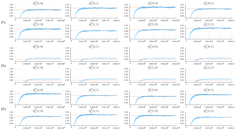
Figure 3: PASQL iterates for different behavioral policies (in blue) and the limit predicted by Thm. 1 (in red).

For each behavioral policy $\mu_{k}$, $k\in\mathsf{K}$, run PASQL for 25 random seeds. The median + interquantile range of the iterates $\{Q^{\ell}_{t}(z,a)\}_{t\geq 1}$ as well as the theoretical limits $Q_{\mu_{k}}(z,a)$ (computed using Thm. 1) are shown in Fig. 3. The salient features of these results are as follows:

• PASQL converges close to the theoretical limit predicted by Thm. 1.

• As highlighted earlier, the limiting value $Q^{\ell}_{\mu_{k}}$ depends on the behavioral policy $\mu_{k}$.

• When the aperiodic behavior policy $\mu_{2}$ is used, the Markov chain $\{(S_{t},Y_{t},Z_{t},A_{t})\}_{t\geq 1}$ is aperiodic, and therefore the limiting distribution $\zeta^{\ell}_{\mu_{2}}$ and the corresponding Q-functions $Q^{\ell}_{\mu_{2}}$ do not depend on $\ell$. This highlights the fact that we have to choose a periodic behavioral policy to converge to a non-stationary policy (PASQL-policy).

Table 1: Performance of converged periodic policies.

$J^{\star}_{2}$	$J^{\pi_{\mu_{1}}}$	$J^{\pi_{\mu_{2}}}$	$J^{\pi_{\mu_{3}}}$
6.793	6.793	1.064	0.532

Comparison of converged policies. Finally, we compute the periodic greedy policy $\pi_{\mu_{k}}=(\pi_{\mu_{k}}^{0},\pi_{\mu_{k}}^{1})$ given by (PASQL-policy), $k\in\mathsf{K}$, and compute its performance $J^{\pi_{\mu_{k}}}$ via policy evaluation on the product space $\mathsf{S}\times\mathsf{Z}$ (see App. G). We also do a brute force search over all $L=2$ periodic deterministic agent-state policies to compute the optimal performance $J^{\star}_{2}$ over all such policies. The results, displayed in Table 1, illustrate the following:

• The greedy policy $\pi_{\mu_{k}}$ depends on the behavioral policy. This is not surprising given the fact that the limiting value $Q^{\ell}_{\mu_{k}}$ depends on $\mu_{k}$.

• The policy $\pi_{\mu_{1}}$ achieves the optimal performance, whereas the policies $\pi_{\mu_{2}}$ and $\pi_{\mu_{3}}$ do not perform well. This highlights the importance of starting with a good behavioral policy. See Sec. 5 for a discussion on variants such as $\epsilon$-greedy.

Table 2: Performance of converged stationary policies.

$J^{\star}_{1}$	$J^{\pi_{\mu_{1}}}$	$J^{\pi_{\mu_{2}}}$	$J^{\pi_{\mu_{3}}}$
2.633	0.0	1.064	2.633

Advantage of learning periodic policies. As stated in the introduction, the main motivation of PASQL is that it allows us to learn non-stationary policies. To see why this is useful, we run ASQL (which is effectively PASQL with $L=1$). We again consider three behavioral policies: $\bar{\mu}_{k}$, $k\in\mathsf{K}\coloneqq\{1,2,3\}$, where $\bar{\mu}_{k}\colon\{0,1\}\to\Delta(\{0,1\})$, where (using similar notation as for $L=2$ case) $\bar{\mu}_{1}\coloneqq[0.2;0.2]$ , $\bar{\mu}_{2}\coloneqq[0.5;0.5]$ , $\bar{\mu}_{3}\coloneqq[0.8;0.8]$ .

For each behavioral policy $\bar{\mu}_{k}$, $k\in\mathsf{K}$, run ASQL for 25 random seeds. The results are shown in App. A.1. The performance of the greedy policies $\pi_{\bar{\mu}_{k}}$ and the performance of the best period $L=1$ deterministic agent-state-based policy computed via brute force is shown in Table 2. The key implications are as follows:

• As was the case for PASQL, the greedy policy $\pi_{\bar{\mu}_{k}}$ depends on the behavioral policy. As mentioned earlier, this is a fundamental consequence of the fact that the agent state is not an information state. Adding (or removing) periodicity does not change this feature.

• The best performance of ASQL is worse than the best performance of PASQL. This highlights the potential benefits of using periodicity. However, at the same time, if a bad behavioral policy is chosen (e.g., policy $\mu_{3}$), the performance of PASQL can be worse than that of ASQL for a nominal policy (e.g., policy $\bar{\mu}_{2}$). This highlights that periodicity is not a magic bullet and some care is needed to choose a good behavioral policy. Understanding what makes a good periodic behavioral policy is an unexplored area that needs investigation.

4 Related work

Policy search for agent state policies. There is a rich literature on planning with agent state-based policies that build on the policy evaluation formula presented in App. G. See [KWW22] for review. These approaches rely on the system model and cannot be used in the RL setting.

State abstractions for POMDPs are related to agent-state based policies. Some frameworks for state abstractions in POMDPs include predictive state representations (PSR) [RGT04, BSG11, HFP14, KJS15a, KJS15, JKS16], approximate bisimulation [CPP09, Cas+21], and approximate information states (AIS) [Sub+22] (which is used in our proof of Thm. 2). Although there are various RL algorithms based on such state abstractions, the key difference is that all these frameworks focus on stationary policies in the infinite horizon setting. Our key insight that non-stationary/periodic policies improve performance is also applicable to these frameworks.

ASQL for POMDPs. As stated earlier, ASQL may be viewed as the special case of PASQL when $L=1$. The convergence of the simplest version of ASQL was established in [SJJ94] for $Z_{t}=Y_{t}$ under the assumption that the actions are chosen i.i.d. (and do not depend on $z_{t}$). In [PP02] it was established that $Q^{0}_{\mu}$ is the fixed point of (ASQL), but convergence of $\{Q_{t}\}_{t\geq 1}$ to $Q^{0}_{\mu}$ was not established. The convergence of ASQL when the agent state is a finite window memory was established in [KY22]. These results were generalized to general agent-state models in [Sey+23]. The regret of an optimistic variant of ASQL was presented in [DVZ22]. However, all of these papers focus on stationary policies.

Our analysis is similar to the analysis of [KY22, Sey+23] with two key differences. First, their convergence results were derived under the assumption that the learning rates are the reciprocal of visitation counts. We relax this assumption to the standard learning rate conditions of Assm. 1 using ideas from stochastic approximation. Second, their analysis is restricted to stationary policies. We generalize the analysis to periodic policies using ideas from time-periodic Markov chains.

Q-learning for non-Markovian environments. As highlighted earlier, a key challenge in understanding the convergence of PASQL is that the agent-state is not Markovian. The same conceptual difficulty arises in the analysis of Q-learning for non-Markovian environments [MH+18, Cha+24, DY24]. Consequently, our analysis has stylistic similarities with the analysis in [MH+18, Cha+24, DY24] but the technical assumptions and the modeling details are different. And more importantly, they restrict attention to stationary policies. Given our results, it may be worthwhile to explore if periodic policies can help in non-Markovian environments as well.

Continual learning and non-stationary MDPs. Non-stationarity is an important consideration in continual learning (see [Abe+24] and references therein). However, in these settings, the environment is non-stationary. Our setting is different: the environment is stationary, but non-stationary policies help because the agent state is not Markov.

Hierarchical learning. The options framework [Pre00, SPS99, Die00, BHP17] is a hierarchical approach that learns temporal abstractions in MDPs and POMDPs. Due to temporal abstraction, the policy learned by the options framework is non-stationary. The same is true for other hierarchical learning approaches proposed in [WS97, CSL21, Vez+17]. In principle, PASQL could be considered as a form of temporal abstraction where time is split into trajectories of length $L$ and then a policy of length $L$ is learned. However, the theoretical analysis for options is mostly restricted to MDP setting and the convergence guarantees for options in POMDPs are weaker [Ste+18, Qia+18, LVC18]. Nonetheless, the algorithmic tools developed for options might be useful for PASQL as well.

Double Q-learning. The update equation of PASQL are structurally similar to the update equations used in double Q-learning  [Has10, VGS16]. However, the motivation and settings are different: the motivation for Double Q-learning is to reduce overestimation bias in off-policy learning in MDPs, while the motivation for PASQL is to induce non-stationarity while learning in POMDPs. Therefore, the analysis of the two algorithms is very different. More importantly, the end goals differ: double Q-learning learns a stationary policy while PASQL learns a periodic policy.

Use of non-stationary/periodic policies in MDPs is investigated in [SL12, LS15, Ber13] in the context of approximate dynamic programming (ADP). Their main result was to show that using non-stationary or periodic policies can improve the approximation error in ADP. Although these results use periodic policies, the setting of ADP in MDPs is very different from ours.

5 Discussion

Deterministic vs. stochastic policies. In this work, we restricted attention to periodic deterministic policies. In principle, we could have also considered periodic stochastic policies. For stationary policies (i.e., when period is one), stochastic policies can outperform deterministic policies [SJJ94] as illustrated by Ex. 3 in App. A.3. However, we do not consider stochastic policies in this work because we are interested in understanding Q-learning with agent-state and Q-learning results in a deterministic policy. There are two options to obtain stochastic policies: using regularization [GSP19], which changes the objective function; or using policy gradient algorithms [Sut+99, BB01], which are a different class of algorithms than Q-learning.

However, as illustrated in the motivating Ex. 2 presented in the introduction, non-stationary policies can do better than stationary stochastic policies as well. So, adding non-stationarity via periodicity remains an interesting research direction when learning stochastic policies as well.

PASQL is a special case of ASQL with state augmentation. In principle, PASQL could be considered as a special case of ASQL with an augmented agent state $\bar{Z}_{t}=(Z_{t},\llbracket t\rrbracket)$. However, the convergence analysis of ASQL in [KY22, Sey+23] does not imply the convergence of PASQL because the results of [KY22, Sey+23] are derived under the assumption that Markov chain $\{(S_{t},Y_{t},Z_{t},A_{t})\}_{t\geq 1}$ is irreducible and aperiodic, while we assume that the Markov chain is periodic. Due to our weaker assumption, we are able to establish convergence of PASQL to time-varying periodic policies.

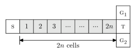
Figure 4: A T-shaped grid world. Agent starts at s, where it learns whether the goal state is $\textsc{g}_{1}$ or $\textsc{g}_{2}$. It has to go through the corridor $\{1,\dots,2n\}$, without knowing where it is, reach t and go up or down to reach the goal state.

Non-stationary policies vs. memory augmentation. Non-stationarity is a fundamentally different concept than memory augmentation. As an illustration, consider the T-shaped grid world shown in Fig. 4, which has a corridor of length $2n$. In App. A.4, we show that for this example, a stationary policy which uses a sliding window of past $m$ observations and actions as the agent state needs a memory of at least $m>2n$ to reach the goal state. In contrast, a periodic policy with period $L=3$ can reach the goal state for every $n$. This example shows that periodicity is a different concept from memory augmentation and highlights the fact that mechanisms other than memory augmentation can achieve optimal behavior.

The analysis of this paper is applicable to general memory augmented policies, so we do not need to choose between memory augmentation and periodicity. Our main message is that once the agent’s memory is fixed based on practical considerations, adding periodicity could improve performance.

Choice of the period $L$. If the agent state $Z_{t}$ is a good approximation to the belief state, then ASQL (or, equivalently, PASQL with $L=1$) would converge to an approximately optimal policy. So, using PASQL a period $L>1$ is useful when the agent state is not a good approximation of the belief state.

As shown by Ex. 2 in the introduction, the performance of the best periodic policy does not increase monotonically with the period $L$. However, if we consider periods in the set $\{n!:n\in\mathds{N}\}$, then the performance increases monotonically. However, PASQL does not necessarily converge to the best periodic policy. The quality of the converged policy (PASQL-policy) depends on the behavior policy $\mu$. The difficulty of finding a good behavioral policy increases with $L$. In addition, increasing the period increases the memory required to store the tuple $(Q^{0},\dots,Q^{L})$ and the number of samples needed to converge (because each component is updated only once every $L$ samples). Therefore, the choice of the period $L$ should be treated as a hyperparameter that needs to be tuned.

Choice of the behavioral policy. The behavioral policy impacts the converged limit of PASQL, and consequently it impacts the periodic greedy policy that is learned. As we pointed out in the discussion after Thm. 1, this dependence is a fundamental consequence of using an agent state that is not Markov and cannot be avoided. Therefore, it is important to understand how to choose behavioral policies that lead to convergence to good policies.

Generalization to other variants. Our analysis is restricted to tabular off-policy Q-learning where a fixed behavioral policy is followed. Our proof fundamentally depends on the fact that the behavioral policy induces a cyclic limiting distribution on the periodic Markov chain $\{(S_{t},Y_{t},A_{t},Z_{t})\}_{t\geq 1}$. Such a condition is not satisfied in variants such as $\epsilon$-greedy Q-learning and SARSA. Generalizing the technical proof to cover these more practical algorithms (including function approximation) is an important future direction.

Appendix A Illustrative examples

A.1 Ex. 1: Learning curves for ASQL

For each behavioral policy $\bar{\mu}_{k}$, $k\in\mathsf{K}$, we run PASQL for 25 random seeds. The median + interquantile range of the iterates $\{Q_{t}(z,a)\}_{t\geq 1}$ as well as the theoretical limits $Q_{\bar{\mu}_{k}}(z,a)$ (computed as per Thm. 1 for $L=1$) are shown in Fig. 5. These curves show that the result of Thm. 1 is valid for the stationary case ($L=1$) as well.

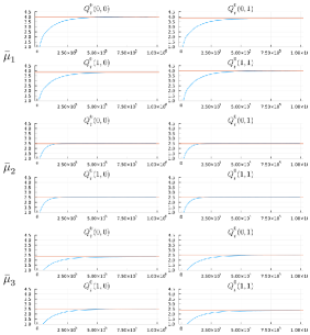
Figure 5: ASQL iterates for different behavioral policies (in blue) and the limit predicted by Thm. 1 (in red).

A.2 Ex. 2: non-stationary policies can outperform stationary policies

Example 2

Consider a POMDP with $\mathsf{S}=\mathds{Z}_{>0}$, $\mathsf{A}=\{0,1\}$, and $\mathsf{Y}=\{0,1\}$. The system starts in an initial state $s_{1}=1$ and has deterministic dynamics. To describe the dynamics and the reward function, we define $\mathsf{D}_{0}\coloneqq\{n(n+1)/2+1:n\in\mathds{Z}_{\geq 0}\}$, $\mathsf{D}_{1}=\mathds{N}\setminus\mathsf{D}_{0}$, and $\mathsf{D}=\mathsf{D}_{0}\times\{0\}\cup\mathsf{D}_{1}\times\{1\}\subset\mathsf{S}\times\mathsf{A}$. Then, the dynamics, observations, and rewards are given by

$$s_{t+1}=\begin{cases}s_{t}+1,&(s_{t},a_{t})\in\mathsf{D},\\ 1,&\hbox{otherwise},\end{cases}\quad y_{t}=\begin{cases}0,&\hbox{$s_{t}$ is odd},\\ 1,&\hbox{$s_{t}$ is even},\end{cases}\quad r(s,a)=\begin{cases}+1,&(s,a)\in\mathsf{D},\\ -1&\hbox{otherwise}.\end{cases}$$ (8)

Thus, the state is incremented if the agent takes action $0$ when the state is in $\mathsf{D}_{0}$ and takes action $1$ when the state is in $\mathsf{D}_{1}$. Taking these actions yield a reward of $+1$. Not taking such an action results in a reward of $-1$ and resets the state to $1$. The agent does not observe the state, but only observes whether the state is odd or even. A graphical representation of the model is shown in Fig. 1. _□

Figure 1: Graphical representation of Ex. 2. The cells indicate the state of the environment. Cells with the same background color have the same observation. The cells with a thick red boundary correspond to elements of the set $\mathsf{D}_{0}\coloneqq\{n(n+1)/2+1:n\in\mathds{N}\}$, where the action $0$ gives a reward of $+1$ and moves the state to the right, while the action $1$ gives a reward of $-1$ and resets the state to $1$. The cells with a thin black boundary correspond to elements of the set $\mathsf{D}_{1}=\mathds{N}\setminus\mathsf{D}_{0}$, where the action $1$ gives the reward of $+1$ and moves the state to the right while the action $0$ gives a reward of $-1$ and resets the state to $1$. Discount factor $\gamma=0.9$.

For policy class $\Pi_{\textsc{{bd}}}$ (the class of all belief-based deterministic policies), since the system starts in a known initial state and the dynamics are deterministic, the agent can compute the current state (thus, the belief is a delta function on the current state). Thus, the agent can always choose the correct action depending on whether the state is in $\mathsf{D}_{0}$ and $\mathsf{D}_{1}$. Hence $J^{\star}_{\textsc{{bd}}}=1/(1-\gamma)$, which is the highest possible reward.

For policy class $\Pi_{\textsc{{sd}}}$ (the class of all agent-state based deterministic policies), there are four possible deterministic policies. For odd observations, the agent may take action $0$ and $1$. Similarly, for even observations, the agent may take action $0$ or $1$. Note that the system starts in state $1$, which is in $\mathsf{D}_{0}$. Therefore, if the agent chooses action $1$ when the observation is odd, it receives a reward of $-1$ and stays at state $1$. Therefore, the discounted total reward is $-1/(1-\gamma)$, which is the least possible value. Therefore, any policy that chooses $1$ on odd observations cannot be optimal. Therefore, the optimal (deterministic) action on odd observations is to pick action $0$. Thus, there are two policies that we need to evaluate.

• If the agent chooses action $0$ at both odd and even observations, the state cycles between $1\to 2\to 3\to 1\to 2\to 3\cdots$ with the reward sequence $(+1,+1,-1,+1,+1,-1,\dots)$. Thus, the cumulative total reward of this policy is $(1+\gamma-\gamma^{2})/(1-\gamma^{3})$.

• If the agent chooses action $0$ at odd observations and action $1$ at even observations, the state cycles between $1\to 2\to 1\to 2\cdots$ with the reward sequence $(+1,-1,+1,-1,\dots)$. Thus, the cumulative total reward of this policy is $1/(1+\gamma)$.

It is easy to verify that for $\gamma\in(0,1)$, $1/(1+\gamma)<(1+\gamma-\gamma^{2})/(1-\gamma^{3})$. Thus,

$$J^{\star}_{\textsc{{sd}}}=\frac{1+\gamma-\gamma^{2}}{1-\gamma^{3}}.$$ (9)

We also consider policy class $\Pi_{\textsc{{ss}}}$: the class of all stationary stochastic agent-state based policies. For policy class $\Pi_{\textsc{{ss}}}$, the policy is characterized by two numbers $(p_{0},p_{1})\in[0,1]^{2}$, where $p_{y}$ denotes the probability of choosing action $1$ when the observation is $y$, $y\in\{0,1\}$. We compute the approximately optimal policy by doing a brute force search over $(p_{0},p_{1})$ by discretizing them two decimal places and for each choice, running a Monte Carlo simulation of length $1,000$ and averaging it over $100$ random seeds. We find that there is negligible difference between the performance of stochastic and deterministic policies.

Finally, we consider policy class $\Pi_{L}$, which is the class of periodic deterministic agent-state based policies. A policy $\pi\in\Pi_{L}$ is characterized by two vectors $p_{0},p_{1}\in\{0,1\}^{L}$, where $p_{y,\ell}$ denotes the action chosen when $t\bmod L=\ell$ and the observation is $y$. We do an exhaustive search over all deterministic policies of length $L$, $L\in\{1,\dots,10\}$ to compute the numbers shown in the main text.

A.3 Ex. 3: stochastic policies can outperform deterministic policies

When the agent state is not an information state, the optimal stochastic stationary policy will perform better than (or equal to) the optimal deterministic stationary policy as observed in [SJJ94]. Here is an example to illustrate this for a simple toy POMDP.

(a) Dynamics under action $0$

(b) Dynamics under action $1$

Figure 6: The dynamics for Ex. 3.

Example 3

Consider a POMDP with $\mathsf{S}=\{0,1,2\}$, $\mathsf{A}=\{0,1\}$ and $\mathsf{Y}=\{0\}$. The system starts at an initial state $s_{1}=0$ and the dynamics under the two actions are shown in Fig. 6. The agent does not observe the state, i.e., $Y_{t}\equiv 0$. The rewards under action $0$ are $r(\cdot,0)=[-1,0,2]$ and the rewards under action $1$ are $r(s,1)=-0.5$, for all $s\in\mathsf{S}$. _□

Figure 7: Performance of stationary stochastic policies ${\pi}_{p}$ for $p\in[0,1]$ for Ex. 3.

We consider agent state $Z_{t}=Y_{t}$. Let $\Pi_{\textsc{{ss}}}$ denote the of all stationary stochastic policies and $\Pi_{\textsc{{sd}}}$ denote the class of of all stationary deterministic policic A policy $\pi\in\Pi_{\textsc{{ss}}}$ is parameterized by a single parameter $p\in[0,1]$, which indicates the probability of choosing action $1$. We denote such a policy by $\pi_{p}$. Note that $p\in\{0,1\}$, $\pi_{p}\in\Pi_{\textsc{{sd}}}$. Let $(P_{a},r_{a})$ denote the probability transition matrix and reward function when $a\in\mathsf{A}$ is chosen and let $(P_{p},r_{p})=(1-p)(P_{0},r_{0})+p(P_{1},r_{1})$. Then, the performance of policy $\pi_{p}$ is given by $J^{\pi_{p}}=[(1-\gamma P_{p})^{-1}r_{p}]_{0}$. The performance for all $p\in[0,1]$ for $\gamma=0.9$ is shown in Fig. 7, which shows that the best performance is achieved by the stochastic policy $\pi_{p}$ with $p\approx 0.39$.

Thus, stochastic policies can outperform deterministic policies.

A.4 Ex. 4: conceptual difference between state-augmentation and periodic policies

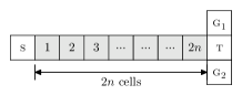
Figure 4: A T-shaped grid world for Ex. 4. In state s, the agent learns about the goal state. In states $\{1,2,\dots,2n\}$, the agent simply knows that it is in the gray corridor, but does not know which cell it is in. In state t, it knows that it has reached the end of corridor and must decide whether to go up or down. The agent gets a reward of $+1$ for reaching the correct goal state and a reward of $-1$ for reaching the wrong goal state.

Example 4

Consider a T-shaped grid world showed in Fig. 4 with state space $\mathsf{P}\times\mathsf{G}$, where $\mathsf{P}=\{\textsc{s},1,2,\dots,2n,\textsc{t}\}$ is the position of the agent and $\mathsf{G}=\{\textsc{g}_{1},\textsc{g}_{2}\}$ is the location of the goal. The observation space is $\mathsf{Y}=\{0,1,2,3\}$. The observation is a deterministic function of the state and is given as follows:

• At state $(\textsc{s},\textsc{g}_{i})$, $i\in\{1,2\}$, the observation is $i$ and reveals the location of the goal state to the agent.

• At states $\{1,\dots,2n\}\times\mathsf{G}$, the observation is $0$, so the agent cannot distinguish between these states.

• At states $\{\textsc{t}\}\times\mathsf{G}$, the observation is $3$, so the agent knows when it reaches the t state.

The action space depends on the current state: actions $\{\textsc{left},\textsc{right},\textsc{stay}\}$ are available when the agent is at $\{\textsc{s},1,\dots,2n\}$ and actions $\{\textsc{up},\textsc{down}\}$ are available at position t.

The agent receives a reward of $+1$ if it reaching the goal state and $-1$ if it reaches the wrong goal state state (i.e., reaches $\textsc{g}_{2}$ when the goal state is $\textsc{g}_{1}$). The discount factor $\gamma=1$. _□

We consider two classes of policies:

1. $\Pi_{\textsc{{sd}}}(m)$: Stationary policies with agent state equal to a sliding window of the last $m$ observations and actions.

2. $\Pi_{L}$: Periodic policies with agent state equal to the last observation and periodic $L$.

It is easy to see that as long as the window length $m\leq 2n$, any policy in $\Pi_{\textsc{{sd}}}(m)$ yields an average return of $0$; for window lengths $m>2n$, the agent can remember the first observation, and therefore it is possible to construct a policy that yields a return of $+1$.

We now consider a deterministic periodic policy with period $L=3$ given as follows: $\pi=(\pi^{0},\pi^{1},\pi^{2})$ where $\pi^{\ell}\colon\mathsf{Y}\to\mathsf{A}$. We denote each $\pi^{\ell}$ as a column vector, where the $y$-th component indicates the action $\pi^{\ell}(y)$, where – means that the choice of the action for that observation is irrelevant for performance. The policy is given by

$$\pi^{0}=\begin{bmatrix}\textsc{right}\\ \textsc{right}\\ \textsc{stay}\\ \textsc{stay}\end{bmatrix},\quad\pi^{1}=\begin{bmatrix}\textsc{right}\\ \text{--}\\ \textsc{right}\\ \textsc{up}\end{bmatrix},\quad\pi^{2}=\begin{bmatrix}\textsc{stay}\\ \text{--}\\ \text{--}\\ \textsc{down}\end{bmatrix}.$$ (10)

It is easy to verify if the system starts in state $(0,\textsc{g}_{1})$, then by following policy $(\pi^{0},\pi^{1},\pi^{2})$, the agent reaches state $\textsc{g}_{1}$ at time $3n+3$. Moreover, when the system starts in state $(0,\textsc{g}_{2})$, then by following the policy $(\pi^{0},\pi^{1},\pi^{2})$, the agent reaches $\textsc{g}_{2}$ at time $3n+4$. Thus, in both cases, the policy $(\pi^{0},\pi^{1},\pi^{2})$ yields the maximum reward of $+1$.

Appendix B Periodic Markov chains

In most of the standard reference material on Markov chains, it is assumed that the Markov chain is aperiodic and irreducible. In our analysis, we need to work with periodic Markov chains. In this appendix, we review some of the basic properties of Markov chains and then derive some fundamental results for periodic Markov chains.

Let $\mathsf{S}$ be a finite set. A stochastic process $\{S_{t}\}_{t\geq 0}$, $S_{t}\in\mathsf{S}$, is called a Markov chain if it satisfies the Markov property: for any $t\in\mathds{Z}_{\geq 0}$ and $s_{1:t+1}\in\mathsf{S}^{t+1}$, we have

$$\mathds{P}(S_{t+1}=s_{t+1}\mid S_{1:t}=s_{1:t})=\mathds{P}(S_{t+1}=s_{t+1}\mid S_{t}=s_{t}).$$ (11)

If is often convenient to assume that $\mathsf{S}=\{1,\dots,n\}$. We can define an $n\times n$ transition probability matrix $P_{t}$ given by $[P_{t}]_{ij}=\mathds{P}(S_{t+1}=j\mid S_{t}=i)$. Then, all the probabilistic properties of the Markov chain is described by the transition matrices $(P_{0},P_{1},\dots)$.

In particular, suppose the Markov chain starts at the initial PMF (probability mass function) $\xi_{0}$ and let $\xi_{t}$ denote the PMF at time $t$. We will view $\xi_{t}$ as a $n$-dimensional row vector. Then, Eq. (11) implies $\xi_{t+1}=\xi_{t}P_{t}$ and, therefore,

$$\xi_{t+1}=\xi_{0}P_{0}P_{1}\cdots P_{t}.$$ (12)

B.1 Time-homogeneous Markov chains and their properties

A Markov chain is said to be time-homogeneous if the transition matrix $P_{t}$ is the same for all time $t$. In this section, we state some standard results for time-homogeneous Markov chains [Nor98].

B.1.1 Classification of states

The states of a time-homogeneous Markov chain can be classified as follows.

1. We say that a state $j$ is accessible from $i$ (abbreviated as $i\rightsquigarrow j$) if there is exists an $m\in\mathds{Z}_{\geq 0}$ (which may depend on $i$ and $j$) such that $[P^{m}]_{ij}>0$. The fact that $[P^{m}]_{ij}>0$ implies that there exists an ordered sequence of states $(i_{0},\dots,i_{m})$ such that $i_{0}=i$ and $i_{m}=j$ such that $P_{i_{k}i_{k+1}}>0$; thus, there is a path of positive probability from state $i$ to state $j$.

   Accessibility is an transitive relationship, i.e., if $i\rightsquigarrow j$ and $j\rightsquigarrow k$ implies that $i\rightsquigarrow k$.

2. Two distinct states $i$ and $j$ are said to communicate (abbreviated to $i\leftrightsquigarrow j$) if $i$ is accessible from $j$ (i.e., $j\rightsquigarrow i$) and $j$ is accessible from $i$ ($i\rightsquigarrow j$). Alternatively, we say that $i$ and $j$ communicate if there exist $m,m^{\prime}\in\mathds{Z}_{\geq 0}$ such that $[P^{m}]_{ij}>0$ and $[P^{m^{\prime}}]_{ji}>0$.

   Communication is an equivalence relationship, i.e., it is reflexive ($i\leftrightsquigarrow i$), symmetric ($i\leftrightsquigarrow j$ if and only if $j\leftrightsquigarrow i$), and transitive ($i\leftrightsquigarrow j$ and $j\leftrightsquigarrow k$ implies $i\leftrightsquigarrow k$).

3. The states in a finite-state Markov chain can be partitioned into two sets: recurrent states and transient states. A state is recurrent if it is accessible from all states that is accessible from it (i.e., $i$ is recurrent if $i\rightsquigarrow j$ implies that $j\rightsquigarrow i$). States that are not recurrent are transient.

   It can be shown that a state $i$ is recurrent if and only if

   $$\sum_{t=1}^{\infty}[P^{t}]_{ii}=\infty.$$ (13)

4. States $i$ and $j$ are said to belong to the same communicating class if $i$ and $j$ communicate. Communicating classes form a partition the state space. Within a communicating class, all states are of the same type, i.e., either all states are recurrent (in which case the class is called a recurrent class) or all states are transient (in which case the class is called a transient class).

   A Markov chain with a single communicating class (thus, all states communicate with each other and are, therefore, recurrent) is called irreducible.

5. The period of a state $i$, denoted by $d(i)$, is defined as

   $$d(i)=\gcd\{t\in\mathds{Z}_{\geq 1}:[P^{t}]_{ii}>0\}.$$ (14)

   If the period is $1$, the state is aperiodic, and if the period is $2$ or more, the state is periodic. It can be shown that all states in the same class have the same period.

   A Markov chain is aperiodic, if all states are aperiodic. A simple sufficient (but not necessary) condition for an irreducible Markov chain to be aperiodic is that there exists a state $i$ such that $P_{ii}>0$. In general, for a finite and aperiodic Markov chain, there exists a positive integer $T$ such that

   $$[P^{t}]_{ii}>0,\quad\forall t\geq T,i\in\mathsf{S}.$$ (15)

B.1.2 Limit behavior of Markov chains

We now state some special distributions for a time-homogeneous Markov chain.

1. A PMF $\zeta$ on $\mathsf{S}$ is called a stationary distribution if $\zeta=\zeta P$. Thus, if a (time-homogeneous) Markov chain starts in a stationary distribution, it stays in a stationary distribution.

   A finite irreducible Markov chain has a unique stationary distribution. Moreover, when the Markov chain is also aperiodic, the stationary distribution is given by $\zeta(j)=1/m_{j}$, where $m_{j}$ is the expected return time to state $j$.

2. A PMF $\zeta$ on $\mathsf{S}$ is called a limiting distribution if

   $$\lim_{t\to\infty}[P^{t}]_{ij}=\zeta(j),\quad\forall i,j\in\mathsf{S}.$$ (16)

   A finite irreducible Markov chain has a limiting distribution if and only if it is aperiodic. Therefore, for an aperiodic Markov chain, the limiting distribution is the same as the stationary distribution.

Theorem 3 (Strong law of large numbers for Markov chains, Theorem 5.6.1 of [Dur19])

Suppose $\{S_{t}\}_{t\geq 1}$ is an irreducible Markov chain that starts in state $i\in\mathsf{S}$. Then,

$$\lim_{T\to\infty}\frac{1}{T}\sum_{t=0}^{T-1}\mathds{1}\{S_{t}=j\}=\frac{1}{m_{j}}.$$ (17)

Therefore, for any function $h\colon\mathsf{S}\to\mathds{R}$,

$$\lim_{T\to\infty}\frac{1}{T}\sum_{t=0}^{T-1}h(S_{t})=\sum_{j\in\mathsf{S}}\frac{h(j)}{m_{j}}.$$ (18)

If, in addition, the Markov chain $\{S_{t}\}_{t\geq 1}$ is aperiodic, and has a limiting distribution $\zeta$, then we have that

$$\lim_{T\to\infty}\frac{1}{T}\sum_{t=0}^{T-1}h(S_{t})=\sum_{j\in\mathsf{S}}\zeta(j)h(j).$$ (19)

_□

B.2 Time-varying with periodic transition matrix

In this section, we consider time-varying Markov chains where the transition matrices $(P_{0},P_{1},\dots)$ are periodic with period $L$. Let $\llbracket t\rrbracket=(t\bmod L)$ and $\mathsf{L}=\{0,\dots,L-1\}$. Then, the transition matrix $P_{t}$ is the same as $P_{\llbracket t\rrbracket}$. Thus, the system dynamics are completely described by the transition matrices $\{P_{\ell}\}_{\ell\in\mathsf{L}}$. With a slight abuse of notation, we will call such a Markov chain as $L$-periodic Markov chain. We will show later that the notion of time-periodicity that we are considering is equivalent to the notion of state-periodicity for time-homogeneous Markov chains defined earlier.

B.3 Constructing an equivalent time-homogeneous Markov chain

Since the Markov chain is not time-homogeneous, the classification and results of the previous section are not directly applicable. There are two ways to construct a time-homogeneous Markov chain: using state augmentation or viewing the process after every $L$ steps.

B.3.1 Method 1: State augmentation

The original time-varying Markov chain $\{S_{t}\}_{t\geq 0}$ is equivalent to the time-homogeneous Markov chain $\{(S_{t},\llbracket t\rrbracket)\}_{t\geq 0}$ defined on $\mathsf{S}\times\mathsf{L}$ with transition matrix $\bar{P}$ given by

$$\bar{P}((s^{\prime},\ell^{\prime})\mid(s,\ell))=P_{\ell}(s^{\prime}\mid s)\mathds{1}\{\ell^{\prime}=\llbracket\ell+1\rrbracket\}.$$ (20)

Example 5

Consider a $2$-periodic Markov chain with state space $\mathsf{S}=\{1,2\}$ and transition matrices

$$P_{0}=\begin{bmatrix}\tfrac{1}{4}&\tfrac{3}{4}\\[5.0pt] \frac{1}{2}&\frac{1}{2}\end{bmatrix}\quad\text{and}\quad P_{1}=\begin{bmatrix}\tfrac{3}{4}&\tfrac{1}{4}\\[5.0pt] \tfrac{1}{4}&\tfrac{3}{4}\end{bmatrix}.$$ (21)

_□

The time-periodic Markov chain of Ex. 5 may be viewed as a time-homogeneous Markov chain with state space $\{1,2\}\times\{0,1\}$ and transition matrix

$$\bar{P}=\hbox{}\;\vbox{\kern 45.02222pt\hbox{$\kern 115.27763pt\kern-4.75pt\left[\kern-115.27763pt\vbox{\kern-45.02222pt\vbox{\halign{$\make@scriptstyle{#}$\hfil\kern 2\p@\kern\@tempdima&\thinspace\hfil$\perhaps@scriptstyle#$\hfil&&\quad\hfil$\perhaps@scriptstyle#$\hfil\cr\hfil\crcr\kern-12.0pt\cr\vbox{\hbox{$\scriptstyle$}}$\hfil\kern 2.0pt\kern 4.75pt&\scriptstyle(1,0)&\scriptstyle(2,0)&\scriptstyle(1,1)&\scriptstyle(2,1)\crcr\kern 2.0pt\cr\vbox{\hbox{$\scriptstyle(1,0)$}}$\hfil\kern 2.0pt\kern 4.75pt&0&0&\tfrac{1}{4}&\tfrac{3}{4}\cr\cr\vbox{\hbox{$\scriptstyle(2,0)$}}$\hfil\kern 2.0pt\kern 4.75pt&0&0&\frac{1}{2}&\frac{1}{2}\cr\cr\vbox{\hbox{$\scriptstyle(1,1)$}}$\hfil\kern 2.0pt\kern 4.75pt&\tfrac{3}{4}&\tfrac{1}{4}&0&0\cr\cr\vbox{\hbox{$\scriptstyle(2,1)$}}$\hfil\kern 2.0pt\kern 4.75pt&\tfrac{1}{4}&\tfrac{3}{4}&0&0\cr\cr}}\kern-12.0pt}\,\right]$}}=\begin{bmatrix}0&I\\ I&0\end{bmatrix}\begin{bmatrix}P_{0}&0\\ 0&P_{1}\end{bmatrix}$$ (22)

where $0$ denotes the all zero matrix and $I$ denotes the identity matrix (both of size $2\times 2$). Note that the time-homogeneous Markov chain is periodic.

Define the following:

• $L$ block diagonal matrices $\Lambda_{0},\dots,\Lambda_{L-1}\in\mathds{R}^{nL\times nL}$ as follows:

  $$\Lambda_{0}=\operatorname{blkdiag}(P_{0},P_{1},\dots,P_{L-1}),\quad\Lambda_{1}=\operatorname{blkdiag}(P_{L-1},P_{0},\dots,P_{L-2}),\quad\text{ etc.}$$ (23)

• A permutation matrix $\Pi\in\{0,1\}^{nL\times nL}$ as follows

  $$\Pi=\begin{bmatrix}0&I&\cdots&0\\ \vdots&\ddots&\ddots&\vdots\\ 0&0&\cdots&I\\ I&0&\cdots&0\end{bmatrix}$$ (24)

  where each block is $n\times n$.

The permutation matrix $\Pi$ satisfies the following properties (which can be verified by direct algebra):

1. $\Pi\,\Pi^{\mathchoice{\raisebox{0.0pt}{$\displaystyle\intercal$}}{\raisebox{0.0pt}{$\textstyle\intercal$}}{\raisebox{0.0pt}{$\scriptstyle\intercal$}}{\raisebox{0.0pt}{$\scriptscriptstyle\intercal$}}}=I$ and therefore $\Pi^{-1}=\Pi^{\mathchoice{\raisebox{0.0pt}{$\displaystyle\intercal$}}{\raisebox{0.0pt}{$\textstyle\intercal$}}{\raisebox{0.0pt}{$\scriptstyle\intercal$}}{\raisebox{0.0pt}{$\scriptscriptstyle\intercal$}}}$.

2. $\Pi^{L}=I$.

3. $\Lambda_{\ell}\Pi=\Pi\Lambda_{\llbracket\ell+1\rrbracket}$, $\ell\in\mathsf{L}$.

In general, the transition matrix of the Markov chain $\{(S_{t},\llbracket t\rrbracket)\}_{t\geq 0}$ is

$$\bar{P}=\begin{bmatrix}0&P_{0}&\cdots&0\\ \vdots&\ddots&\ddots&\vdots\\ 0&0&\cdots&P_{L-2}\\ P_{L-1}&0&\cdots&0\end{bmatrix}_{nL\times nL}=\Lambda_{0}\Pi.$$ (25)

B.3.2 Method 2: Viewing the process every $L$ steps

The original Markov chain viewed every $L$-steps, i.e., the process $\{S_{kL+\ell}\}_{k\geq 0}$, $\ell\in\mathsf{L}$, is a time-homogeneous Markov chain with transition probability matrix $\mathcal{P}_{\ell}$ given by

$$\mathcal{P}_{\ell}=P_{\llbracket\ell\rrbracket}P_{\llbracket\ell+1\rrbracket}\cdots P_{\llbracket\ell+L-1\rrbracket}$$ (26)

that is,

$$\mathcal{P}_{0}=P_{0}P_{1}\cdots P_{L-2}P_{L-1},\quad\mathcal{P}_{1}=P_{1}P_{2}\cdots P_{L-1}P_{0},\quad\text{etc.}$$ (27)

B.3.3 Relationship between the two constructions

The two constructions are related as follows.

Proposition 1

We have that $\bar{P}^{L}=\operatorname{blkdiag}(\mathcal{P}_{0},\dots,\mathcal{P}_{L}).$ _□

Proof

From (P3), we get that $\bar{P}=\Pi\Lambda_{1}$. Therefore,

$$\bar{P}^{2}=\Lambda_{0}\Pi\Lambda_{0}\Pi=\Lambda_{0}\Lambda_{1}\Pi^{2}$$ (28)

Similarly

$$\bar{P}^{3}=\Lambda_{0}\Pi\bar{P}^{2}=\Lambda_{0}\Pi\Lambda_{0}\Lambda_{1}\Pi^{2}=\Lambda_{0}\Lambda_{1}\Pi\Lambda_{1}\Pi^{2}=\Lambda_{0}\Lambda_{1}\Lambda_{2}\Pi^{3}$$ (29)

Continuing this way, we get

$$\bar{P}^{L}=\Lambda_{0}\Lambda_{1}\dots\Lambda_{L-1}\Pi^{L}=\Lambda_{0}\Lambda_{1}\dots\Lambda_{L-1}.$$ (30)

where the last equality follows from (P2). The result then follows from the definitions of $\Lambda_{\ell}$ and $\mathcal{P}_{\ell}$, $\ell\in\mathsf{L}$. $\Box$ _■

B.4 Limiting behavior of periodic Markov chain

In the subsequent discussion, we consider the following assumptions.

Assumption 3

Every $\{\mathcal{P}_{\ell}\}$, $\ell\in\mathsf{L}$, is irreducible and aperiodic

Suppose Assm. 3 holds. Define $\zeta^{\ell}$ to be the unique stationary distribution for Markov chain $\mathcal{P}_{\ell}$, $\ell\in\mathsf{L}$, i.e., $\zeta^{\ell}$ is the unique PMF that satisfies $\zeta^{\ell}=\zeta^{\ell}\mathcal{P}_{\ell}$.

Proposition 2

The PMFs $\{\zeta^{\ell}\}_{\ell\in\mathsf{L}}$ satisfy

$$\zeta^{\ell}P_{\ell}=\zeta^{\llbracket\ell+1\rrbracket},\quad\ell\in\mathsf{L}.$$ (31)

_□

Proof

We prove the result for $\ell=0$. The analysis is the same for general $\ell$. By assumption, we have that

$$\zeta^{0}=\zeta^{0}\mathcal{P}_{0}=\zeta^{0}P_{0}P_{1}\cdots P_{L-1}.$$ (32)

Let $\bar{\zeta}^{1}\coloneqq\zeta^{0}P_{0}$. Then, we have

$$\bar{\zeta}^{1}=\zeta^{0}P_{0}=\zeta^{0}P_{0}P_{1}\cdots P_{L-1}P_{0}=\bar{\zeta}^{1}P_{1}\cdots P_{L-1}P_{0}=\bar{\zeta}^{1}\mathcal{P}_{1}.$$ (33)

Thus $\bar{\zeta}^{1}$ is a stationary distribution. Since $\mathcal{P}_{1}$ is irreducible, the stationary distribution is unique, hence $\bar{\zeta}^{1}$ must equal $\zeta^{1}$. $\Box$ _■

We can verify this result for Ex. 5. For this model, we have

$$\mathcal{P}_{0}=P_{0}P_{1}=\begin{bmatrix}\frac{3}{8}&\frac{5}{8}\\[5.0pt] \frac{1}{2}&\frac{1}{2}\end{bmatrix}\quad\text{and}\quad\mathcal{P}_{1}=P_{1}P_{0}=\begin{bmatrix}\frac{5}{16}&\frac{11}{16}\\[5.0pt] \frac{7}{16}&\frac{9}{16}\end{bmatrix}.$$ (34)

Thus,

$$\zeta^{0}=\begin{bmatrix}\frac{4}{9}&\frac{5}{9}\end{bmatrix}\quad\text{and}\quad\zeta^{1}=\begin{bmatrix}\frac{7}{18}&\frac{11}{18}\end{bmatrix}$$ (35)

And we can verify that $\zeta^{0}P_{0}=\zeta^{1}$ and $\zeta^{1}P_{1}=\zeta^{0}$.

Proposition 3

Under Assm. 3, the limiting distribution of the Markov chain $\{S_{t}\}_{t\geq 0}$ is cyclic. In particular, for any initial distribution $\xi_{0}$,

$$\lim_{k\to\infty}\xi_{kL+\ell}=\zeta^{\ell}$$ (36)

Furthermore,

$$\limsup_{K\to\infty}\frac{1}{K}\sum_{k=0}^{K-1}\mathds{1}\{S_{kL+\ell}=i\}=[\zeta^{\ell}]_{i},\quad\forall i\in\mathsf{S},\ell\in\mathsf{S}.$$ (37)

Consequently, for any function $h\colon\mathsf{S}\to\mathds{R}$,

$$\limsup_{K\to\infty}\frac{1}{K}\sum_{k=0}^{K-1}h(S_{kL+\ell})=\sum_{s\in\mathsf{S}}h(s)[\zeta^{\ell}]_{s},\quad\ell\in\mathsf{S}.$$ (38)

_□

Proof

The results follow from standard results for the time-homogeneous Markov chain $\{S_{kL+\ell}\}_{k\geq 0}$. $\Box$ _■

Proof (Alternative)

We present an alternative proof that uses the state augmented Markov chain $\bar{P}$. We first prove that under Assm. 3, the chain $\bar{P}$ is irreducible periodic with period $L$.

The proof of irreducibility relies on two observations.

1. Fix an $\ell\in\mathsf{L}$ and consider $i,j\in\mathsf{S}$. Since $\mathcal{P}_{\ell}$ is irreducible, we have that there exists a positive integer $m$ (depending on $i$, $j$, and $\ell$) such that $[\mathcal{P}_{\ell}^{m}]_{ij}>0$. Note that Prop. 1 implies that $[\bar{P}^{mL}]_{(i,\ell),(j,\ell)}=[\mathcal{P}_{\ell}]_{ij}>0$. Therefore, in the Markov chain $\bar{P}$, states $(i,\ell)\rightsquigarrow(j,\ell)$. Since $i$ and $j$ were arbitrary, all states $\mathsf{S}\times\{\ell\}$ belong to the same communicating class.

2. Now consider two $\ell,\ell^{\prime}\in\mathsf{L}$. Suppose we start at some state $(i,\ell)\in\mathsf{S}\times\{\ell\}$, then in $[\ell^{\prime}-\ell]$ steps, we will reach some state $(j,\ell^{\prime})\in\mathsf{S}\times\{\ell^{\prime}\}$. Thus, $(j,\ell^{\prime})$ is accessible from $(i,\ell)$. But, we have already argued that all states in $\mathsf{S}\times\{\ell\}$ belong to the same communicating class, therefore all states in $\mathsf{S}\times\{\ell^{\prime}\}$ are accessible from all states in $\mathsf{S}\times\{\ell\}$. By interchanging the roles of $\ell$ and $\ell^{\prime}$, we have that all states in $\mathsf{S}\times\{\ell\}$ are accessible from all starts in $\mathsf{S}\times\{\ell^{\prime}\}$. Therefore, the states $\mathsf{S}\times\{\ell\}$ and $\mathsf{S}\times\{\ell^{\prime}\}$ belong to the same communicating class. Since $\ell$ and $\ell^{\prime}$ were arbitrary, we have that all states of $\bar{P}$ belong to the same communicating class. Hence, $\bar{P}$ is irreducible.

We now show that $\bar{P}$ is periodic. First observe that the Markov chain starting in the set $\mathsf{S}\times\{\ell\}$ does not return to the same set for the first $L-1$ steps. Thus, $[\bar{P}^{t}]_{(i,\ell),(i,\ell)}=0$ for $t\in\{1,2,\dots,L-1\}$. Therefore, the only possible values of $t$ for which $[\bar{P}^{t}]_{(i,\ell),(i,\ell)}>0$ are those that are multiples of $L$. Hence, for any $(i,\ell)\in\mathsf{S}\times\mathsf{L}$,

$$d(i,\ell)=\gcd\{t\in\mathds{Z}_{\geq 1}:[\bar{P}^{t}]_{(i,\ell),(i,\ell)}>0\}=L\gcd\{k\in\mathds{Z}_{\geq 1}:[\mathcal{P}_{\ell}^{k}]_{ii}>0\}$$ (39)

Moreover, since $\mathcal{P}_{\ell}$ is aperiodic, $\gcd\{k\in\mathds{Z}_{\geq 1}:[\mathcal{P}_{\ell}^{k}]_{ii}>0\}=1$. Substituting in (39), we get that $d(i,\ell)=L$ for all $(i,\ell)$. Thus, all states have a period of $L$.

Now, from Prop. 1, we know that $\bar{P}^{L}=\operatorname{blkdiag}(\mathcal{P}_{0},\dots,\mathcal{P}_{L-1})$. Therefore

$$\lim_{k\to\infty}[\bar{P}^{kL}]_{(i,\ell),(j,\ell)}=[\zeta^{\ell}]_{j},\quad(i,\ell)\in\mathsf{S}\times\mathsf{L}.$$ (40)

Consequently, if we start with an initial distribution $\bar{\xi}_{0}$ such that $\bar{\xi}_{0}(\mathsf{S}\times\{0\})=1$, then,

$$\lim_{k\to\infty}\bar{\xi}_{kL}=\operatorname{vec}(\zeta_{0},0,\dots,0)$$ (41)

where the $0$ vectors are of size $n$. Consequently, Prop. 2 implies that

$$\lim_{k\to\infty}\bar{\xi}_{kL+\ell}=\operatorname{vec}(0,\dots,0,\zeta_{\ell},0,\dots,0),\quad\forall\ell\in\mathsf{L}$$ (42)

where $\zeta^{\ell}$ is the $\ell$-th place. This completes the proof of (36).

Now consider the function $\bar{h}\colon\mathsf{S}\times\mathsf{L}\to\mathds{R}$ defined as $\bar{h}(s,\ell^{\prime})=h(s)\mathds{1}\{\ell^{\prime}=\ell\}$. Then, by taking $T=KL$, we have

$$\lim_{K\to\infty}\frac{1}{K}\sum_{t=0}^{K-1}h(S_{kL+\ell})=\lim_{T\to\infty}\frac{L}{T}\sum_{t=0}^{T-1}\bar{h}(S_{t},\llbracket t\rrbracket)=L\sum_{s\in\mathsf{S}}\frac{h(s)}{m_{(s,\ell)}}$$ (43)

where the last equation uses (18) from Thm. 3. Now, (38) follows from observing that mean return time to state $(s,\ell)$ in Markov chain $\bar{P}$ is $L$ times the mean-return time to state $s$ in Markov chain $\mathcal{P}_{\ell}$, which equals $1/[\zeta^{\ell}]_{s}$ since $\mathcal{P}_{\ell}$ is irreducible and aperiodic. $\Box$ _■

Appendix C Periodic Markov decision processes

Periodic MDPs are a special class time non-stationary MDPs where the dynamics and rewards are periodic. In particular, let $\mathcal{M}$ be a time-varying MDP with state space $\mathsf{S}$, action space $\mathsf{A}$, and dynamics and reward at time $t$ given by $P_{t}\colon\mathsf{S}\times\mathsf{A}\to\Delta(\mathsf{S})$ and $r_{t}\colon\mathsf{S}\times\mathsf{A}\to\mathds{R}$.

As before, we use $\llbracket t\rrbracket$ to denote $t\bmod L$ and $\mathsf{L}$ to denote $\{0,\dots,L-1\}$. The MDP $\mathcal{M}$ is periodic with period $L$ if there exist $(P^{\ell},r^{\ell})$, $\ell\in\mathsf{L}$ such that for all $t$:

$$P_{t}(S_{t+1}\mid S_{t},A_{t})=P^{\llbracket t\rrbracket}(S_{t+1}\mid S_{t},A_{t})\quad\text{and}\quad r_{t}(S_{t},A_{t})=r^{\llbracket t\rrbracket}(S_{t},A_{t}).$$ (44)

Periodic MDPs were first considered in [Rii65]. Periodic MDPs may be viewed as stationary MDPs by considering the augmented state $(S_{t},\llbracket t\rrbracket)$. By this equivalence, it can be shown that there is no loss of optimality in restricting attention to periodic policies. In particular, let $(V^{0},\dots,V^{L-1})$ denote the fixed point of the following system of equations

$$V^{\ell}(s)=\max_{a\in\mathsf{A}}\Bigl{\{}r^{\ell}(s,a)+\gamma\sum_{s^{\prime}\in\mathsf{S}}P^{\ell}(s^{\prime}|s,a)V^{\llbracket\ell+1\rrbracket}(s^{\prime})\Bigr{\}},\quad\forall(\ell,s,a)\in\mathsf{L}\times\mathsf{S}\times\mathsf{A}.$$ (45)

Define $\pi^{\ell}_{\star}(s)$ to be the arg-max or the right hand side of (45). Then the time-varying policy $\pi=(\pi_{1},\pi_{2},\dots)$ given by $\pi_{t}=\pi^{\llbracket t\rrbracket}_{\star}$ is optimal.

See [Sch16] for a discussion of how to modify standard MDP algorithms to solve periodic dynamic program (45).

Appendix D Stochastic Approximation with Markov noise

We now state a generalization of Thm. 3 to stochastic approximation style iterations.

Theorem 4

Let $\{S_{t}\}_{t\geq 1}$, $\mathsf{S}$, be an irreducible and aperiodic finite Markov chain with unique limiting distribution $\zeta$. Let $\mathcal{F}_{t}$ denote the natural filtration w.r.t. $\{S_{t}\}_{t\geq 1}$ and $\{\alpha_{t}\}_{t\geq 1}$ be a non-negative real-valued process adapted to $\{\mathcal{F}_{t}\}$ that satisfies

$$\sum_{t\geq 1}\alpha_{t}=\infty\quad\text{and}\quad\sum_{t\geq 1}\alpha_{t}^{2}<\infty.$$ (46)

Consider the iterative process $\{X_{t}\}_{t\geq 1}$, where $X_{1}$ is arbitrary and for $t\geq 1$, we have

$$X_{t+1}=(1-\alpha_{t})X_{t}+\alpha_{t}h(S_{t})$$ (47)

Then, the sequence $\{X_{t}\}_{t\geq 1}$ converges almost surely to limit. In particular,

$$\lim_{T\to\infty}X_{T}=\sum_{s\in\mathsf{S}}h(s)\zeta(s),\quad a.s.$$ (48)

_□

Eq. (47) is similar to standard stochastic approximation iteration [RM51, KY97, Bor08], which the “noise sequence” $h(S_{t})$ is assumed to be a martingale difference sequence. The setting considered above is sometimes referred to as stochastic approximation with Markov noise. In fact, more general version of this result where the noise sequence is allowed to depend on the state $X_{t}$ are typically established in the literature [BMP12, Bor08, KY97, PB24]. For the sake of completeness, we will show that Thm. 4 is a special case of these more-general results.

Before presenting the proof, we point out that Thm. 4 is a generalization of Thm. 3, Eq. (19). In particular, suppose the learning rates are $\alpha_{t}=1/(1+t)$. Then, simple algebra shows that

$$X_{T}=\frac{1}{T}\sum_{t=1}^{T}h(S_{t}).$$ (49)

Then, (19) of Thm. 3 implies that the limit is given by the right had side of (48). Therefore, Thm. 4 is a generalization of Thm. 3 to general learning rates which satisfy (46).

Proof

To establish the result, we will show that the iteration $\{X_{t}\}_{t\geq 1}$ satisfies the assumptions for the convergence of stochastic approximation with (state dependent) Markov noise and stochastic recursive inclusions given in [PB24, Theorem 2.7]. The proof is due to [BP24]. In particular, we can rewrite (47) as

$$X_{t+1}=X_{t}+\alpha_{t}g(X_{t},S_{t})$$ (50)

where $g(x,s)=-x+h(s)$. Moreover, for ease of notation, define $\bar{h}=\sum_{s\in\mathsf{S}}h(s)\zeta(s)$. Then, we have

• $g(x,s)$ is Lipschtiz continuous in the first argument, so A2.14 of [PB24] holds.

• From (19), the ergodic occupation measure of $\{h(S_{t})\}_{t\geq 1}$ is $\{\bar{h}\}$, which is compact and convex. So, A2.15 of [PB24] is satisfied.

• There is no “martingale noise” in (50), so A2.16 of [PB24] holds trivially.

• Eq. (46) is equivalent to A2.17 of [PB24].

• To check A2.18 of [PB24], for any measure $\nu$ on $\mathsf{S}$, define

  $$\tilde{h}(x,\nu)=\int g(x,s)\nu(ds)=-x+\bar{h}.$$ (51)

  Also define

  $$\tilde{h}_{c}(x,\nu)=\frac{\tilde{h}(cx,c\nu)}{c}=-x+\frac{\bar{h}}{c}$$ (52)

  Let $\tilde{h}_{\infty}(x,\nu)=\lim_{c\to\infty}h_{c}(x,\nu)==x$. Thus, the differential inclusion in A2.18(ii) is actually an ODE

  $$\dot{x}=-x$$ (53)

  which has origin as the unique global asymptotically stable equilibrium point. Thus, A2.18 of [PB24] is satisfied.

Therefore, all assumptions of Theorem 2.7 of [PB24] are satisfied. Therefore, by that result, the iterates $\{X_{t}\}_{t\geq 1}$ converge to solution of the ODE (note that the differential inclusion in Theorem 2.7 of [PB24] is an ODE in our setting)

$$\dot{x}=-x+\bar{h}.$$ (54)

Note that $x=\bar{h}$ is the unique asymptotically stable attractor of the ODE (54). Therefore, Theorem 2.7 of [PB24] implies (48). $\Box$ _■

Thm. 4 also implies the following generalization of Prop. 3.

Proposition 4

Suppose $\{S_{t}\}_{t\geq 1}$ is a time-periodic Markov chain with period $L$ that satisfies Assm. 3 with the unique limiting distribution $\{\zeta^{\ell}\}_{\ell\in\mathsf{L}}$. Let $\{\mathcal{F}_{t}\}_{t\geq 1}$ denote the natural filtration w.r.t. $\{S_{t}\}_{t\geq 1}$ and $\{\alpha^{\ell}_{t}\}_{t\geq 1}$, $\ell\in\mathsf{L}$, be non-negative real-valued processes adapted to $\{\mathcal{F}_{t}\}_{t\geq 1}$ such that $\alpha^{\ell}_{t}=0$ when $\ell\neq\llbracket t\rrbracket$ and

$$\sum_{t\geq 1}\alpha^{\ell}_{t}=\infty\quad\text{and}\quad\sum_{t\geq 1}(\alpha_{t}^{\ell})^{2}<\infty.$$ (55)

Fix any $\ell\in\mathsf{L}$, Consider the iterative process $\{X^{\ell}_{k}\}_{k\geq 1}$, where $X_{1}$ is arbitrary and for $k\geq 1$, we have

$$X^{\ell}_{t+1}=(1-\alpha^{\ell}_{t})X^{\ell}_{t}+\alpha^{\ell}_{t}h(S_{t})$$ (56)

Then, the sequence $\{X^{\ell}_{t}\}_{t\geq 1}$ converges almost surely to the following limit

$$\lim_{t\to\infty}X^{\ell}_{t}=\sum_{s\in\mathsf{S}}h(s)\zeta^{\ell}(s),\quad a.s.$$ (57)

_□

Proof

Note that the learning rates used here can be viewed as the learning rates of $L$ separated stochastic iterations on a common timescale $t$. Each separate stochastic iteration $\ell\in\mathsf{L}$ is actually only updated once every $L$ steps on the timescale $t$. Because of the condition $\alpha^{\ell}_{t}=0$ when $\ell\neq\llbracket t\rrbracket$, each update is followed by $L-1$ “pseudo”-updates where the learning rate is $0$. Therefore, each $X^{\ell}$ is updated only once every $L$ steps on timescale $t$.

The result then follows immediately from Thm. 4 by considering the process $\{S_{t}\}_{t\geq 1}$ every $L$ steps for each $\ell\in\mathsf{L}$. $\Box$ _■

Appendix E Thm. 1: Convergence of periodic Q-learning

The high-level idea of the proof is similar to [KY22] for ASQL when the agent state is a finite window of past observations and action. The key observation of the [KY22] is the following: Consider an iterative process $X_{t+1}=(1-\alpha_{t})X_{t}+\alpha_{t}U_{t}$ with the learning rates $\alpha_{t}=1/(1+t)$. Then, $X_{t+1}=(X_{0}+\sum_{\tau=1}^{t}U_{t})/(1+t)$. Then, if the process $\{U_{t}\}_{t\geq 1}$ has an ergodic limit (e.g., when $\{U_{t}\}_{t\geq 1}$ is a function of a Markov chain, see Thm. 3), the process $\{X_{t}\}_{t\geq 1}$ converges to the ergodic limit of $\{U_{t}\}_{t\geq 1}$. We follow a similar idea but with the following changes:

• Instead of assuming “averaging” learning rates (i.e., reciprocal of the number of visits), we allow for general learning rates of Assm. 1.

• We account for the fact that that the “noise” is periodic.

The rest of the analysis then follows along the standard argument of convergence of Q-learning [JSJ94, KY22, DY24].

Define the error function $\Delta^{\ell}_{t+1}=Q^{\ell}_{t+1}-Q^{\ell}_{\mu}$, for all $\ell\in\mathsf{L}$. To prove Thm. 1, it suffices to prove that $\lVert\Delta^{\ell}_{t}\rVert\to 0$ for all $\ell\in\mathsf{L}$, where $\lVert\cdot\rVert$ is the supremum-norm. The proof proceeds in three steps.

E.1 Step 1: State splitting of the error function

Define $V_{t}^{\ell}(z)\coloneqq\max_{a\in\mathsf{A}}Q_{t}^{\ell}(z,a)$ and $V_{\mu}^{\ell}(z)\coloneqq\max_{a\in\mathsf{A}}Q^{\ell}_{\mu}(z,a)$, for all $\ell\in\mathsf{L}$, $z\in\mathsf{Z}$. We can combine (PASQL), (3), and (4) as follows

$$\Delta^{\ell}_{t+1}(z,a)=(1-\alpha^{\ell}_{t}(z,a))\Delta^{\ell}_{t}(z,a)+\alpha^{\ell}_{t}(z,a)\bigl{[}U^{\ell,1}_{t}(z,a)+U^{\ell,2}_{t}(z,a)\bigr{]}$$ (58)

where

$$U^{\ell,1}_{t}(z,a) \coloneqq r(S_{t},A_{t})-r^{\ell}_{\mu}(z,a)+\gamma V_{\mu}^{\llbracket\ell+1\rrbracket}(Z_{t+1})-\gamma\sum_{z^{\prime}\in\mathsf{Z}}P^{\ell}_{\mu}(z^{\prime}|z,a)V_{\mu}^{\llbracket\ell+1\rrbracket}(z^{\prime}),$$ (59)

$$U^{\ell,2}_{t}(z,a) \coloneqq\gamma V_{t}^{\llbracket\ell+1\rrbracket}(Z_{t+1})-\gamma V^{\llbracket\ell+1\rrbracket}_{\mu}(Z_{t+1}).$$ (60)

For each $\ell\in\mathsf{L}$, Eq. (58) may be viewed as a linear system with state $\Delta^{\ell}_{t+1}$ and two inputs $U^{\ell,1}_{t}$ and $U^{\ell,2}_{t}$. We exploit the linearity of the system and split the state into two components: $\Delta^{\ell}_{t+1}=X^{\ell,0}_{t+1}+X^{\ell,1}_{t+1}$, where the two components evolve as follows:

$$X^{\ell,i}_{t+1}(z,a)=(1-\alpha^{\ell}_{t}(z,a))X^{\ell,i}_{t}(z,a)+\alpha^{\ell}_{t}(z,a)U^{\ell,i}_{t}(z,a),\quad i\in\{1,2\}$$ (61)

Linearity implies that (58) is equivalent to (61). We will now separately show that $\lVert X^{\ell,1}_{t}\rVert\to 0$ and $\lVert X^{\ell,2}_{t}\rVert\to 0$.

E.2 Step 2: Convergence of component $X^{\ell,1}_{t}$

Fix $(\ell,z,a)\in\mathsf{L}\times\mathsf{Z}\times\mathsf{A}$. Define the function

$$h^{\ell}(S_{t},Z_{t},A_{t},Z_{t+1})=\bigl{[}r(S_{t},A_{t})-r^{\ell}_{\mu}(Z_{t},A_{t})\bigr{]}+\Bigl{[}\gamma V^{\llbracket\ell+1\rrbracket}(Z_{t+1})-\gamma\sum_{z^{\prime}\in\mathsf{Z}}P^{\ell}_{\mu}(z^{\prime}|Z_{t},A_{t})V^{\llbracket\ell+1\rrbracket}_{\mu}(z^{\prime})\Bigr{]}.$$ (62)

Then, Prop. 4 implies that the sequence $\{X^{\ell,1}_{t}\}_{t\geq 1}$ converges almost surely to the limit

$$\sum_{(s,z_{+})\in\mathsf{S}\times\mathsf{Z}}\zeta^{\ell}_{\mu}(s,z,a,z_{+})h^{\ell}(s,z,a,z_{+})$$ (63)

where $\zeta^{\ell}_{\mu}(s,z,a,z_{+})=\zeta^{\ell}_{\mu}(s,z,a)P^{\ell}_{\mu}(z_{+}|z,a)$. Furthermore, the Strong Law of Large numbers for periodic Markov chains (Prop. 3, Eq. (37)) implies that the term in (63) converges almost surely to zero.

Hence, for all $(\ell,z,a)$, the process $\{X^{\ell,1}_{t}(z,a)\}_{t\geq 1}$ converges to zero almost surely.

E.3 Step 3: Convergence of component $X^{\ell,2}_{t}$

The remaining analysis is similar to corresponding step in the standard convergence proof of Q-learning and its variations [JSJ94, KY22, DY24].

Arbitrarily fix a $\epsilon>0$. In the previous step, we have shown that $\lVert X^{\ell,1}_{t}\rVert\to 0$ a.s. Therefore, there exists a set $\Omega^{1}$ of measure one and a constant $T(\omega,\epsilon)$ such that for $\omega\in\Omega^{1}$, all $t>T(\omega,\epsilon)$, and $(z,a)\in\mathsf{Z}\times\mathsf{A}$, we have

$$X^{\ell,1}_{t}(z,a)<\epsilon.$$ (64)

Now pick a constant $C$ such that

$$\kappa\coloneqq\gamma\left(1+\frac{1}{C}\right)<1$$ (65)

Suppose for some $t>T(\omega,\epsilon)$, $\lVert X^{\ell,2}_{t}\rVert>C\epsilon$, i.e., $\epsilon<\lVert X^{\ell,2}\rVert/C$. Then, for any $(z,a)\in\mathsf{Z}\times\mathsf{A}$,

$$U^{\ell,2}_{t}(z,a) \leq\gamma\lVert V^{\ell}_{t}-V^{\ell}_{\mu}\rVert\leq\gamma\lVert Q^{\ell}_{t}-Q^{\ell}_{\mu}\rVert=\gamma\lVert\Delta_{t}\rVert$$ (66a)

$$\leq\gamma\lVert X^{\ell,1}_{t}\rVert+\gamma\lVert X^{\ell,2}_{t}\rVert\leq\gamma\epsilon+\gamma\lVert X^{\ell,2}_{t}\rVert$$ (66b)

$$\leq\gamma\left(1+\frac{1}{C}\right)\lVert X^{\ell,2}_{t}\rVert=\kappa\lVert X^{\ell,2}_{t}\rVert<\lVert X^{\ell,2}_{t}\rVert.$$ (66c)

Thus, for any $t>T(\omega,\epsilon)$ and $\lVert X^{\ell,2}_{t}\rVert>C\epsilon$, we have

$$X^{\ell,2}_{t+1}(z,a)=(1-\alpha^{\ell}_{t}(z,a))X^{\ell,2}_{t}(z,a)+\alpha^{\ell}_{t}(z,a)U^{\ell,2}_{t}(z,a)<\lVert X^{\ell,2}_{t}\rVert.$$ (67)

Hence, when $\lVert X^{\ell,2}_{t}\rVert>C\epsilon$, it decreases monotonically. Hence, there are two possibilities: either (i) $\lVert X^{\ell,2}_{t}\rVert$always remains above $C\epsilon$; or (ii) it goes below $C\epsilon$ at some stage. We consider these two possibilities separately.

E.3.1 Possibility (i): $\lVert X^{\ell,2}_{t}\rVert$ always remains above $C\epsilon$

We will show that $\lVert X^{\ell,2}_{t}\rVert$ cannot remain above $C\epsilon$ for ever. We first start with a basic result for random iterations. This is a self-contained result, so we reuse some of the variables used in the rest of the paper.

Lemma 2

Let $\{X_{t}\}_{t\geq 1}$, $\{Y_{t}\}_{t\geq 1}$, and $\{\alpha_{t}\}_{t\geq 1}$ be non-negative sequences adapted to a filtration $\{\mathcal{F}_{t}\}_{t\geq 1}$ that satisfy the following:

$$X_{t+1} \leq(1-\alpha_{t})X_{t},$$ (68a)

$$Y_{t+1} \leq(1-\alpha_{t})Y_{t}+\alpha_{t}c,$$ (68b)

where $c$ is a constant. Suppose

$$\sum_{t=1}^{\infty}\alpha_{t}=\infty$$ (69)

Then, the sequence $\{X_{t}\}_{t\geq 1}$ converges to zero almost surely and the sequence $\{Y_{t}\}_{t\geq 1}$ converges to $c$ almost surely. _□

Proof

The iteration (68a) implies that

$$X_{t+1}\leq\Bigl{[}(1-\alpha_{1})\cdots(1-\alpha_{t})\Bigr{]}X_{1}$$ (70)

Condition (69) implies that the term in the square brackets converges to zero. Therefore, $X_{t}\to 0$.

Observe that the iteration (68b) can be rewritten as

$$Y_{t+1}-c\leq(1-\alpha_{t})(Y_{t}-c)$$ (71)

which is of the form (68a). Therefore, $Y_{t}-c\to 0$. $\Box$ _■

We will now prove that $\lVert X^{\ell,2}_{t}\rVert$ cannot remain above $C\epsilon$ forever. The proof is by contraction. Suppose $\lVert X^{\ell,2}_{t}\rVert$ remains above $C\epsilon$ forever. As argued earlier, this implies that $\lVert X^{\ell,2}_{t}\rVert$, $t\geq T(\omega,\epsilon)$ is a strictly decreasing sequence, so it must be bounded from above. Let $B^{(0)}$ be such that $\lVert X^{\ell,2}_{t}\rVert\leq B^{(0)}$ for all $t\geq T(\omega,\epsilon)$. Eq. (66c) implies that $\lVert U^{\ell,2}_{t}\rVert\leq\kappa B^{(0)}$. Thus,

$$X^{\ell,2}_{t+1}(z,a)\leq(1-\alpha^{\ell}_{t}(z,a))\lVert X^{\ell,2}_{t}\rVert+\alpha^{\ell}_{t}(z,a)\lVert U^{\ell,2}_{t}\rVert\leq(1-\alpha^{\ell}_{t}(z,a))\lVert X^{\ell,2}_{t}\rVert+\alpha^{\ell}_{t}(z,a)\kappa\lVert X^{\ell,2}_{t}\rVert$$ (72)

which implies that $\lVert X^{\ell,2}_{t}\rVert\leq\lVert M^{\ell,(0)}_{t}\rVert$, where $\{M^{\ell,(0)}_{t}\}_{t\geq T(\omega,\epsilon)}$ is a sequence given by

$$M^{\ell,(0)}_{t+1}(z,a)\leq(1-\alpha^{\ell}_{t}(z,a))M^{\ell,(0)}_{t}(z,a)+\alpha^{\ell}_{t}(z,a)\kappa B^{(0)},\quad\forall(z,a)\in\mathsf{Z}\times\mathsf{A}.$$ (73)

Lem. 2 implies that $M^{\ell,(0)}_{t}(z,a)\to\kappa B^{(0)}$ and hence $\lVert M^{\ell,(0)}_{t}\rVert\to\kappa B^{(0)}$. Now pick an arbitrary $\bar{\epsilon}\in(0,(1-\kappa)C\epsilon)$. Thus, there exists a time $T^{(1)}=T^{(1)}(\omega,\epsilon,\bar{\epsilon})$ such that for all $t>T^{(1)}$, $\lVert M^{\ell,(0)}_{t}\rVert\leq B^{(1)}\coloneqq\kappa B^{(0)}+\epsilon$. Since $\lVert X^{\ell,2}_{t}\rVert$ is bounded by $\lVert M^{\ell,(0)}_{t}\rVert$, this implies that for all $t>T^{(1)}$, $\lVert X^{\ell,2}_{t}\rVert\leq B^{(1)}$ and, by (66c), $\lVert U^{\ell,2}_{t}\rVert\leq\kappa B^{(1)}$. By repeating the above argument, there exists a time $T^{(2)}$ such that for all $t\geq T^{(2)}$,

$$\lVert X^{\ell,2}_{t}\rVert\leq B^{(2)}\coloneqq\kappa B^{(1)}+\bar{\epsilon}=\kappa^{2}B^{(0)}+\kappa\bar{\epsilon}+\bar{\epsilon},$$ (74)

and so on. By (65), $\kappa<1$ and $\bar{\epsilon}$ is chosen to be less than $C\epsilon$. So eventually, $B^{(m)}\coloneqq\kappa^{m}B^{(0)}+\kappa^{m-1}\bar{\epsilon}+\cdots+\bar{\epsilon}$ must get below $C\epsilon$ for some $m$, contradicting the assumption that $\lVert X^{\ell,2}_{t}\rVert$ remains above $C\epsilon$ forever.

E.3.2 Possibility (ii): $\lVert X^{\ell,2}_{t}\rVert$ goes below $C\epsilon$ at some stage

Suppose that there is some $t>T(\omega,\epsilon)$ such that $\lVert X^{\ell,2}_{t}\rVert<C\epsilon$. Then (66b) implies that

$$\lVert U^{\ell,2}_{t}\rVert\leq\gamma\lVert X^{\ell,1}_{t}\rVert+\gamma\lVert X^{\ell,2}_{t}\rVert\leq\gamma\epsilon+\gamma C\epsilon<C\epsilon$$ (75)

where the last inequality uses (65). Therefore,

$$X^{\ell,2}_{t+1}(z,a)\leq(1-\alpha^{\ell}_{t}(z,a))\lVert X^{\ell,2}_{t}\rVert+\alpha^{\ell}_{t}(z,a)\lVert U^{\ell,2}_{t}\rVert<C\epsilon$$ (76)

where the last inequality uses the fact that both $\lVert U^{\ell,2}_{t}\rVert$ and $\lVert X^{\ell,2}_{t}\rVert$ are both below $C\epsilon$. Thus, we have that

$$\lVert X^{\ell,2}_{t}\rVert<C\epsilon.$$ (77)

Hence, once $\lVert X^{\ell,2}_{t}\rVert$ goes below $C\epsilon$, it stays there.

E.3.3 Implication

We have show that for sufficiently large $t>T(\omega,\epsilon)$, $\lVert X^{\ell,2}_{t}\rVert<C\epsilon$. Since $\epsilon$ is arbitrary, this means that for all $\omega\in\Omega^{1}$, $\lVert X^{\ell,2}_{t}\rVert\to 0$. Thus,

$$\lim_{t\to\infty}\lVert X^{\ell,2}_{t}\rVert=0,\quad a.s.$$ (78)

E.4 Putting everything together

Recall that we defined $\Delta^{\ell}_{t}=Q^{\ell}_{t}-Q_{\mu}$ and split $\Delta^{\ell}_{t}=X^{\ell,1}_{t}+X^{\ell,2}_{t}$. Step 2 shows that $\lVert X^{\ell,1}_{t}\rVert\to 0$, a.s. and Eq. (78) shows that $\lVert X^{\ell,2}_{t}\rVert\to 0$, a.s. Thus, by triangle inequality,

$$\lim_{t\to\infty}\lVert\Delta^{\ell}_{t}\rVert\leq\lim_{t\to\infty}\lVert X^{\ell,1}_{t}\rVert+\lim_{t\to\infty}\lVert X^{\ell,2}_{t}\rVert=0,$$ (79)

which establishes that $Q^{\ell}_{t}\to Q_{\mu}$, a.s.

Appendix F Thm. 2: Sub-optimality gap

The high-level idea of proving Thm. 2 is as follows. Thm. 1 shows that PASQL converges to a cyclic limit, which is the solution to a periodic MDP. Thus, the question of characterizing the sub-optimality gap is equivalent to the following. Given a PODMP $\mathcal{P}$, let $\mathcal{M}$ be a periodic agent-state based model that approximates the reward and the dynamics of $\mathcal{P}$ (in the sense of an approximate information state, as defined in [Sub+22]). Let $\hat{\pi}^{\star}$ be the optimal policy of model $\mathcal{M}$. What is the sub-optimality gap when $\hat{\pi}^{\star}$ is used in the original POMDP $\mathcal{P}$?

To answer such questions, a general framework of approximate information states was developed in [Sub+22] for both finite and infinite horizon models. However, we cannot directly used the results of [Sub+22] because the infinite horizon results there were restricted to stationary policies, while we are interested in the sub-optimality gap of periodic policies.

Nonetheless, Thm. 2 can be proved by building on the existing results of [Sub+22]. In particular, we start by looking at finite horizon model rather than infinite horizon model. Then, as per [Sub+22, Definition 7], the agent state process may be viewed as an approximate information state with approximation errors $\{(\varepsilon_{t},\delta_{t})\}_{t\geq 1}$, where

$$\varepsilon_{t} =\sup_{h_{t},a_{t}}\Bigl{\lvert}\mathds{E}[R_{t}\mid h_{t},a_{t}]-\sum_{s\in\mathsf{S}}r(s,a)\zeta_{\mu}^{\llbracket t\rrbracket}(s\mid z,a)\Bigr{\rvert},$$ (80)

$$\delta_{t} =\sup_{h_{t},a_{t}}d_{\mathfrak{F}}(\mathds{P}(Z_{t+1}=\cdot\mid h_{t},a_{t}),P^{\llbracket t\rrbracket}_{\mu}(Z_{t+1}=\cdot|\sigma_{t}(h_{t}),a_{t})).$$ (81)

Let $V^{\vec{\pi}}_{t,T}(h_{t})=\mathds{E}^{\vec{\pi}}\bigl{[}\sum_{\tau=t}^{T}\gamma^{\tau-1}R_{\tau}\mid h_{t}\bigr{]}$ denote the value function of policy $\vec{\pi}$ for the finite horizon model starting at history $h_{t}$ at time $t$. Let $V^{\star}_{t,T}(h_{t})\coloneqq\sup_{\vec{\pi}}V^{\vec{\pi}}_{t,T}(h_{t})$ denote the optimal value function, where the optimization is over all history dependent policies. Moreover, let $\hat{V}_{t,T}(z_{t})$ denote the optimal value function for the periodic MDP model constructed in Thm. 1. Let $\vec{\pi}_{\mu}$ denote the history-based policy defined in Sec. 2.4.

Then, from [Sub+22, Theorem 9] we have

$$\sup_{h_{t}}\bigl{[}V^{\star}_{t,T}(h_{t})-V^{\vec{\pi}_{\mu}}_{t,T}(h_{t})\bigr{]}\leq 2\sum_{\tau=t}^{T}\gamma^{\tau-t}\bigl{[}\varepsilon_{\tau}+\gamma\delta_{\tau}\rho_{\mathfrak{F}}(\hat{V}_{\tau+1,T})\bigr{]}$$ (82)

where we set $\hat{V}_{T+1,T}(z)\equiv 0$ for convenience.

The following hold when we let $T\to\infty$.

• Since $R_{t}$ is uniformly bounded, $V^{\star}_{t,T}(h_{t})\to V^{\star}_{t}(h_{t})$ as $T\to\infty$.

• By the same argument, $V^{\vec{\pi}_{\mu}}_{t,T}(h_{t})\to V^{\vec{\pi}_{\mu}}_{t}(h_{t})$ as $T\to\infty$.

• By standard results for periodic MDPs (see App. C), $\hat{V}_{t,T}\to V^{\llbracket t\rrbracket}_{\mu}$ as $T\to\infty$.

• By definition, $\varepsilon_{t}\leq\varepsilon_{t}^{\llbracket t\rrbracket}$ and $\delta_{t}\leq\delta_{t}^{\llbracket t\rrbracket}$.

Therefore, by taking $T\to\infty$ in (82), we get

$$\sup_{h_{t}}\bigl{[}V^{\star}_{t}(h_{t})-V^{\vec{\pi}_{\mu}}_{t}(h_{t})\bigr{]}\leq 2\sum_{\tau=t}^{\infty}\gamma^{\tau-t}\bigl{[}\varepsilon^{\llbracket\tau\rrbracket}_{\tau}+\gamma\delta_{\tau}^{\llbracket\tau\rrbracket}\rho_{\mathfrak{F}}(\hat{V}^{\llbracket\tau+1\rrbracket})\bigr{]}.$$ (83)

The result then follows from observing that for $\tau\in\mathsf{T}(t,\ell)$, $\epsilon_{t}^{\ell}$ and $\delta_{t}^{\ell}$ are non-decreasing sequences.

Appendix G Policy evaluation of an agent-state based policy

The performance of any agent-state based policy can be evaluated via a slight generalization of “cross-product MDP” method originally presented in [Pla77]. This method has been rediscovered in slightly different forms multiple times [Lit96, Cas98, Hau97, Han98].

The key intuition is Lem. 1. Thus, for any agent-state based policy, $\{(S_{t},Z_{t})\}_{t\geq 1}$ is a Markov chain. The only difference in our setting is that the Markov chain is time-periodic. Thus, for any periodic agent-state based policy $(\pi^{0},\dots,\pi^{L-1})$, we can identify the periodic rewards $(\bar{r}^{0}_{,}\dots,\bar{r}^{L-1})$ and periodic dynamics $(\bar{P}^{0},\dots,\bar{P}^{L-1})$ (which depend on $\pi$ but we are not carrying that dependence in our notation) as follows:

$$\bar{r}^{\ell}(s,z) =\sum_{a\in\mathsf{A}}\pi^{\ell}(a|z)r(s,a),$$ (84)

$$\bar{P}^{\ell}(s^{\prime},z^{\prime}|s,z) =\sum_{(y,a)\in\mathsf{Y}\times\mathsf{A}}\pi^{\ell}(a|z)P(s^{\prime},y^{\prime}|s,a)\mathds{1}_{\{z^{\prime}=\phi(z,y^{\prime},a)\}}.$$ (85)

We can then evaluate the performance of this time-periodic Markov chain via performance evaluation formulas for periodic MDPs (App. C). In particular, define

$$\tilde{r} =\bar{r}^{0}+\gamma\bar{P}^{0}\bar{r}^{1}+\dots+\gamma^{L-1}\bar{P}^{0}\bar{P}^{1}\cdots\bar{P}^{L-2}\bar{r}^{L-1},$$ (86)

$$\tilde{P} =\bar{P}^{0}\bar{P}^{1}\cdots\bar{P}^{L-1},$$ (87)

to be the $L$-step cumulative rewards and dynamics for the time-periodic Markov chain. Then define

$$\tilde{V}=(1-\gamma^{L}\tilde{P})^{-1}\tilde{r}$$ (88)

Thus, $\tilde{V}(s,z)$ gives the performance of periodic policy $\pi$ when starting at initial state $(s,z)$. If the initial state is stochastic, we can average over the initial distribution.

Appendix H Reproducibility information

The hyperparameters for the numerical experiments presented in Sec. 3 are shown in Table 3. The experiments were run in a computer cluster by running jobs that requested $2$-CPU nodes with $<8$GB memory. Each seed typically took less than $10$ minutes to execute.

Table 3: Hyperparameters used in Ex. 1

Parameter	Value
Training steps	$10^{6}$
Start learn rate	$10^{-3}$
End learn rate	$10^{-5}$
Learn rate schedule	Exponential
Exponential decay rate	1.0
Number of random seeds	25

References

- [Abe+24] David Abel, André Barreto, Benjamin Van Roy, Doina Precup, Hado P Hasselt and Satinder Singh “A definition of continual reinforcement learning” In Advances in Neural Information Processing Systems 36, 2024
- [Åst65] K.J Åström “Optimal Control of Markov Processes with Incomplete State Information” In Journal of Mathematical Analysis and Applications 10.1, 1965, pp. 174–205
- [BHP17] Pierre-Luc Bacon, Jean Harb and Doina Precup “The option-critic architecture” In Proceedings of the AAAI conference on artificial intelligence 31.1, 2017
- [BB01] Jonathan Baxter and Peter L Bartlett “Infinite-horizon policy-gradient estimation” In Journal of Artificial Intelligence Research 15, 2001, pp. 319–350
- [BMP12] Albert Benveniste, Michel Métivier and Pierre Priouret “Adaptive algorithms and stochastic approximations” Springer Science & Business Media, 2012
- [BT96] Dimitri Bertsekas and John N Tsitsiklis “Neuro-dynamic programming” Athena Scientific, 1996
- [Ber13] Dimitri P Bertsekas “Abstract Dynamic Programming” Athena Scientific, 2013
- [BP24] Shalabh Bhatnagar and L.A. Prashanth Personal communication, 2024
- [BSG11] Byron Boots, Sajid M Siddiqi and Geoffrey J Gordon “Closing the learning-planning loop with predictive state representations” In The International Journal of Robotics Research 30.7, 2011, pp. 954–966
- [Bor08] Vivek S Borkar “Stochastic approximation: a dynamical systems viewpoint” Hindustan Book Agency, 2008
- [CLZ97] Anthony Cassandra, Michael L. Littman and Nevin L. Zhang “Incremental pruning: A simple, fast, exact method for partially observable Markov decision processes” In Uncertainty in Artificial Intelligence, 1997
- [CKL94] Anthony R Cassandra, Leslie Pack Kaelbling and Michael L Littman “Acting optimally in partially observable stochastic domains” In AAAI Conference on Artificial Intelligence 94, 1994, pp. 1023–1028
- [Cas98] Anthony Rocco Cassandra “Exact and approximate algorithms for partially observable Markov decision processes”, 1998
- [Cas+21] Pablo Samuel Castro, Tyler Kastner, Prakash Panangaden and Mark Rowland “Mico: Improved representations via sampling-based state similarity for Markov decision processes” In Advances in Neural Information Processing Systems 34, 2021, pp. 30113–30126
- [CPP09] Pablo Samuel Castro, Prakash Panangaden and Doina Precup “Equivalence Relations in Fully and Partially Observable Markov Decision Processes” In International Joint Conference on Artificial Intelligence, 2009, pp. 1653–1658
- [Cha+24] Siddharth Chandak, Pratik Shah, Vivek S Borkar and Parth Dodhia “Reinforcement learning in non-Markovian environments” In Systems & Control Letters 185 Elsevier, 2024, pp. 105751
- [CSL21] Elliot Chane-Sane, Cordelia Schmid and Ivan Laptev “Goal-conditioned reinforcement learning with imagined subgoals” In International Conference on Machine Learning, 2021, pp. 1430–1440 PMLR
- [Cha07] Joseph Chang “Stochastic Processes” Unpublished. Availale at http://www.stat.yale.edu/~pollard/Courses/251.spring2013/Handouts/Chang-notes.pdf, 2007
- [DY24] Ali Devran Kera and Serdar Yüksel “Q-Learning for Stochastic Control under General Information Structures and Non-Markovian Environments” In Transactions on Machine Learning Research, 2024
- [Die00] Thomas G Dietterich “Hierarchical reinforcement learning with the MAXQ value function decomposition” In Journal of Artificial Intelligence Research 13 AI Access Foundation, 2000, pp. 227–303
- [DRZ22] Shi Dong, Benjamin Van Roy and Zhengyuan Zhou “Simple Agent, Complex Environment: Efficient Reinforcement Learning with Agent States” In Journal of Machine Learning Research 23.255, 2022, pp. 1–54
- [DVZ22] Shi Dong, Benjamin Van Roy and Zhengyuan Zhou “Simple agent, complex environment: Efficient reinforcement learning with agent states” In Journal of Machine Learning Research 23.255, 2022, pp. 1–54
- [Dur19] Rick Durrett “Probability: Theory and Examples” Cambridge University Press, 2019 DOI: 10.1017/9781108591034
- [GSP19] Matthieu Geist, Bruno Scherrer and Olivier Pietquin “A theory of regularized markov decision processes” In International Conference on Machine Learning, 2019, pp. 2160–2169 PMLR
- [Gru+18] Audrunas Gruslys, Rémi Munos, Ivo Danihelka, Marc G. Bellemare and Alex Graves “The Reactor: A Sample-Efficient Actor-Critic Architecture” In Proceedings of the International Conference on Learning Representations (ICLR), 2018 URL: https://arxiv.org/abs/1704.04651
- [Haf+20] Danijar Hafner, Timothy Lillicrap, Jimmy Ba and Mohammad Norouzi “Dream to Control: Learning Behaviors by Latent Imagination” In International Conference on Learning Representations, 2020
- [Haf+21] Danijar Hafner, Timothy P Lillicrap, Mohammad Norouzi and Jimmy Ba “Mastering Atari with Discrete World Models” In International Conference on Learning Representations, 2021
- [HFP14] William Hamilton, Mahdi Milani Fard and Joelle Pineau “Efficient learning and planning with compressed predictive states” In The Journal of Machine Learning Research 15.1, 2014, pp. 3395–3439
- [Han98] Eric A. Hansen “Solving POMDPs by searching in policy space” In Uncertainty in Artificial Intelligence, 1998, pp. 211–219
- [Has10] Hado Hasselt “Double Q-learning” In Advances in neural information processing systems 23, 2010
- [HS15] Matthew Hausknecht and Peter Stone “Deep recurrent Q-learning for partially observable MDPs” In AAAI Fall Symposium Series, 2015
- [Hau97] Milos Hauskrecht “Planning and control in stochastic domains with imperfect information”, 1997
- [Hau00] Milos Hauskrecht “Value-function approximations for partially observable Markov decision processes” In Journal of artificial intelligence research 13, 2000, pp. 33–94
- [JSJ94] Tommi Jaakkola, Satinder Singh and Michael Jordan “Reinforcement Learning Algorithm for Partially Observable Markov Decision Problems” In Advances in Neural Information Processing Systems 7 MIT Press, 1994, pp. 345–352
- [JKS16] Nan Jiang, Alex Kulesza and Satinder P Singh “Improving Predictive State Representations via Gradient Descent.” In AAAI Conference on Artificial Intelligence, 2016, pp. 1709–1715
- [Kap+19] Steven Kapturowski, Georg Ostrovski, Will Dabney, John Quan and Remi Munos “Recurrent Experience Replay in Distributed Reinforcement Learning” In International Conference on Learning Representations, 2019
- [KY22] Ali Devran Kara and Serdar Yüksel “Convergence of Finite Memory Q Learning for POMDPs and Near Optimality of Learned Policies Under Filter Stability” In Mathematics of Operations Research INFORMS, 2022 DOI: 10.1287/moor.2022.1331
- [KWW22] Mykel J Kochenderfer, Tim A Wheeler and Kyle H Wray “Algorithms for decision making” MIT press, 2022
- [KJS15] Alex Kulesza, Nan Jiang and Satinder Singh “Low-rank spectral learning with weighted loss functions” In Artificial Intelligence and Statistics, 2015, pp. 517–525
- [KJS15a] Alex Kulesza, Nan Jiang and Satinder P Singh “Spectral Learning of Predictive State Representations with Insufficient Statistics.” In AAAI Conference on Artificial Intelligence, 2015, pp. 2715–2721
- [KY97] Harold J. Kushner and G. Yin “Stochastic Approximation Algorithms and Applications” Springer New York, 1997 DOI: 10.1007/978-1-4899-2696-8
- [LVC18] Tuyen P Le, Ngo Anh Vien and TaeChoong Chung “A deep hierarchical reinforcement learning algorithm in partially observable Markov decision processes” In Ieee Access 6 IEEE, 2018, pp. 49089–49102
- [LS15] Boris Lesner and Bruno Scherrer “Non-Stationary Approximate Modified Policy Iteration” In International Conference on Machine Learning 37, Proceedings of Machine Learning Research Lille, France: PMLR, 2015, pp. 1567–1575
- [Lit96] Michael Lederman Littman “Algorithms for sequential decision-making”, 1996
- [Lu+23] Xiuyuan Lu, Benjamin Van Roy, Vikranth Dwaracherla, Morteza Ibrahimi, Ian Osband and Zheng Wen “Reinforcement learning, bit by bit” In Foundations and Trends in Machine Learning 16.6 Now Publishers, Inc., 2023, pp. 733–865
- [MH+18] Sultan Javed Majeed and Marcus Hutter “On Q-learning Convergence for Non-Markov Decision Processes.” In IJCAI 18, 2018, pp. 2546–2552
- [Mni+13] Volodymyr Mnih, Koray Kavukcuoglu, David Silver, Alex Graves, Ioannis Antonoglou, Daan Wierstra and Martin Riedmiller “Playing atari with deep reinforcement learning” In arXiv preprint arXiv:1312.5602, 2013
- [Mül97] Alfred Müller “Integral probability metrics and their generating classes of functions” In Advances in Applied Probability 29.2, 1997, pp. 429–443
- [Nor98] James R Norris “Markov chains” Cambridge University Press, 1998
- [PP02] Theodore J. Perkins and Mark D. Pendrith “On the Existence of Fixed Points for Q-Learning and Sarsa in Partially Observable Domains” In International Conference on Machine Learning San Francisco, CA, USA: Morgan Kaufmann Publishers Inc., 2002, pp. 490–497
- [PGT+03] Joelle Pineau, Geoff Gordon and Sebastian Thrun “Point-based value iteration: An anytime algorithm for POMDPs” In International Joint Conference on Artificial Intelligence 3, 2003, pp. 1025–1032
- [Pla77] Loren Kerry Platzman “Finite Memory Estimation and Control of Finite Probabilistic Systems.”, 1977
- [PB24] L.A. Prashanth and Shalabh Bhatnagar “Gradient-based algorithms for zeroth-order optimization” Now publishers, 2024 URL: http://www.cse.iitm.ac.in/~prashla/bookstuff/GBSO_book.pdf
- [Pre00] Doina Precup “Temporal abstraction in reinforcement learning” University of Massachusetts Amherst, 2000
- [Qia+18] Zhiqian Qiao, Katharina Muelling, John Dolan, Praveen Palanisamy and Priyantha Mudalige “Pomdp and hierarchical options mdp with continuous actions for autonomous driving at intersections” In 2018 21st International Conference on Intelligent Transportation Systems (ITSC), 2018, pp. 2377–2382 IEEE
- [Rii65] Jens Ove Riis “Discounted Markov Programming in a Periodic Process” In Operations Research 13.6 INFORMS, 1965, pp. 920–929 DOI: 10.1287/opre.13.6.920
- [RM51] Herbert Robbins and Sutton Monro “A Stochastic Approximation Method” In The Annals of Mathematical Statistics 22.3 Institute of Mathematical Statistics, 1951, pp. 400–407
- [RGT04] Matthew Rosencrantz, Geoff Gordon and Sebastian Thrun “Learning low dimensional predictive representations” In International Conference on Machine Learning, 2004
- [Sch16] Bruno Scherrer “On Periodic Markov Decision Processes”, European Workshop on Reinforcement Learning, 2016 URL: https://ewrl.files.wordpress.com/2016/12/scherrer.pdf
- [SL12] Bruno Scherrer and Boris Lesner “On the use of non-stationary policies for stationary infinite-horizon Markov decision processes” In Advances in Neural Information Processing Systems 25, 2012
- [Sey+23] Erfan SeyedSalehi, Nima Akbarzadeh, Amit Sinha and Aditya Mahajan “Approximate information state based convergence analysis of recurrent Q-learning” In European conference on reinforcement learning, 2023 URL: https://arxiv.org/abs/2306.05991
- [Sil+16] David Silver et al. “Mastering the game of Go with deep neural networks and tree search” In Nature 529, 2016, pp. 484–489
- [SJJ94] Satinder P Singh, Tommi Jaakkola and Michael I Jordan “Learning without state-estimation in partially observable Markovian decision processes” In Machine Learning Elsevier, 1994, pp. 284–292
- [SS73] Richard D. Smallwood and Edward J. Sondik “The Optimal Control of Partially Observable Markov Processes over a Finite Horizon” In Operations Research 21.5 INFORMS, 1973, pp. 1071–1088 DOI: 10.1287/opre.21.5.1071
- [SS04] Trey Smith and Reid Simmons “Heuristic search value iteration for POMDPs” In Conference on Uncertainty in Artificial Intelligence, 2004, pp. 520–527
- [SV05] Matthijs TJ Spaan and Nikos Vlassis “Perseus: Randomized point-based value iteration for POMDPs” In Journal of Artificial Intelligence Research 24, 2005, pp. 195–220
- [Ste+18] Denis Steckelmacher, Diederik Roijers, Anna Harutyunyan, Peter Vrancx, Hélène Plisnier and Ann Nowé “Reinforcement learning in POMDPs with memoryless options and option-observation initiation sets” In Proceedings of the AAAI conference on artificial intelligence 32.1, 2018
- [Sub+22] Jayakumar Subramanian, Amit Sinha, Raihan Seraj and Aditya Mahajan “Approximate information state for approximate planning and reinforcement learning in partially observed systems” In Journal of Machine Learning Research 23.12, 2022, pp. 1–83
- [Sut+99] Richard S Sutton, David McAllester, Satinder Singh and Yishay Mansour “Policy gradient methods for reinforcement learning with function approximation” In Advances in Neural Information Processing Systems 12, 1999
- [SPS99] Richard S Sutton, Doina Precup and Satinder Singh “Between MDPs and semi-MDPs: A framework for temporal abstraction in reinforcement learning” In Artificial intelligence 112.1-2 Elsevier, 1999, pp. 181–211
- [SB08] Richard S. Sutton and Andrew G. Barto “Reinforcement Learning: An Introduction” MIT Press, 2008
- [VGS16] Hado Van Hasselt, Arthur Guez and David Silver “Deep reinforcement learning with double q-learning” In Proceedings of the AAAI conference on artificial intelligence 30.1, 2016
- [Vez+17] Alexander Sasha Vezhnevets, Simon Osindero, Tom Schaul, Nicolas Heess, Max Jaderberg, David Silver and Koray Kavukcuoglu “Feudal networks for hierarchical reinforcement learning” In International conference on machine learning, 2017, pp. 3540–3549 PMLR
- [WS94] Chelsea C White III and William T Scherer “Finite-memory suboptimal design for partially observed Markov decision processes” In Operations Research 42.3 INFORMS, 1994, pp. 439–455
- [WS97] Marco Wiering and Jürgen Schmidhuber “HQ-learning” In Adaptive behavior 6.2 Sage Publications Sage CA: Thousand Oaks, CA, 1997, pp. 219–246
- [Wie+07] Daan Wierstra, Alexander Foerster, Jan Peters and Juergen Schmidhuber “Solving deep memory POMDPs with recurrent policy gradients” In International Conference on Artificial Neural Networks (ICANN), 2007, pp. 697–706 Springer
- [Wie+10] Daan Wierstra, Alexander Förster, Jan Peters and Jürgen Schmidhuber “Recurrent policy gradients” In Logic Journal of the IGPL 18.5, 2010, pp. 620–634
- [Wit75] Hans S Witsenhausen “On policy independence of conditional expectations” In Information and Control 28.1 Elsevier, 1975, pp. 65–75
- [Zha09] H. Zhang “Partially Observable Markov Decision Processes: A Geometric Technique and Analysis” In Operations Research, 2009