Sketchy Moment Matching: Toward Fast and Provable Data Selection for Finetuning

Abstract

We revisit data selection in a modern context of finetuning from a fundamental perspective. Extending the classical wisdom of variance minimization in low dimensions to high-dimensional finetuning, our generalization analysis unveils the importance of additionally reducing bias induced by low-rank approximation. Inspired by the variance-bias tradeoff in high dimensions from the theory, we introduce Sketchy Moment Matching (SkMM), a scalable data selection scheme with two stages. (i) First, the bias is controlled using gradient sketching that explores the finetuning parameter space for an informative low-dimensional subspace $\mathcal{S}$; (ii) then the variance is reduced over $\mathcal{S}$ via moment matching between the original and selected datasets. Theoretically, we show that gradient sketching is fast and provably accurate: selecting $n$ samples by reducing variance over $\mathcal{S}$ preserves the fast-rate generalization $O(\dim(\mathcal{S})/n)$, independent of the parameter dimension. Empirically, we concretize the variance-bias balance via synthetic experiments and demonstrate the effectiveness of SkMM for finetuning in real vision tasks.

1 Introduction

As the data volume and training cost explode with the unprecedented model performance, the long-standing problem of data selection [30, 4] is getting increasing attention in the modern context of deep learning from various perspectives, including data pruning [70, 89], coreset selection [30, 90, 88, 54, 6, 41], and data filtering [66, 27, 4, 83, 38]. A common goal shared by these perspectives is to train a model from scratch on less data to learn high-quality representations and achieve competitive generalization. However, empirical observations also suggest the limitation of data removal during pre-training: a seemingly inevitable tradeoff between less computation and higher-quality representations [2, 29]. While existing works on data selection have a dominating focus on the training-from-scratch setting, the sensitivity of representation learning to data and the growing availability of powerful pre-trained models calls for attention to a less studied [87] but equally important problem: data selection for finetuning.

In the simplest finetuning setting—linear probing on low-dimensional representations, data selection falls in the classical frames of coreset selection for linear regression [85, 65, 3, 63, 11, 46, 19, 69] and optimal experimental design [8, 61, 26, 82, 5] where the generalization gap can be reduced by selecting data that minimize the associated variance. However, for high-dimensional finetuning, variance minimization alone is insufficient to characterize the generalization due to the overparametrized nature of modern architectures. Even for linear probing, when the parameter dimension $r$ is higher than the sample size $n$, the selected data necessarily fails to capture a subspace of the parameter space with dimension at least $r-n$, leading to errors in addition to variance. Nevertheless, the prevailing empirical and theoretical evidence [76, 2] on the ubiquitous intrinsic low-dimensional structures of high-dimensional data/model motivates a natural question:

Can the low intrinsic dimension be leveraged in data selection for high-dimensional finetuning?

Low intrinsic dimension leads to variance-bias tradeoff in data selection.

We provide a positive answer to this question through a variance-bias tradeoff perspective. Intuitively, we consider a low-dimensional subspace ${\mathcal{S}}$ in the finetuning parameter space where the model learns the necessary knowledge for the downstream task. The generalization gap can be controlled by simultaneously reducing the bias (redundant information) by “exploring” the finetuning parameter space to find a suitable ${\mathcal{S}}$ and the variance by “exploiting” the useful knowledge in ${\mathcal{S}}$.

Given the high-dimensional nature of the finetuning parameter space, direct search for such suitable subspace ${\mathcal{S}}$ is computationally infeasible in general. This leads to a follow-up question:

How to explore the intrinsic low-dimensional structure efficiently for data selection?

We propose a two-stage solution—Sketchy Moment Matching (SkMM): (i) dimensionality reduction via gradient sketching to efficiently explore the finetuning parameter space, and (ii) variance control via moment matching to exploit useful knowledge in the low-dimensional subspace.

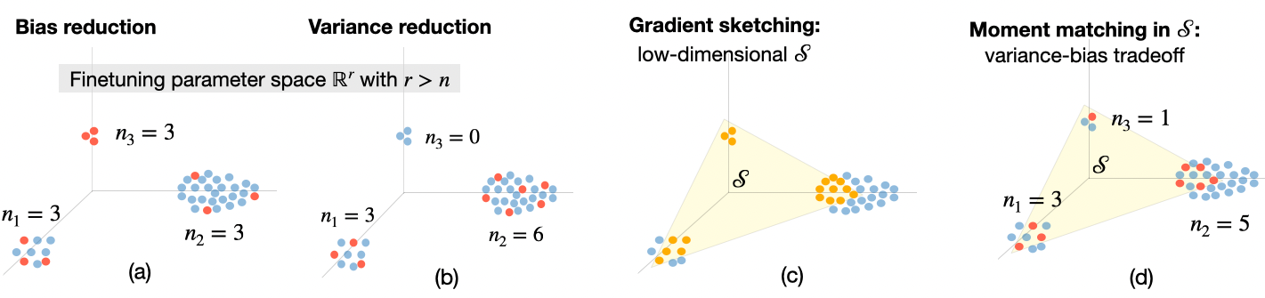
Figure 1: Controlling variance-bias tradeoff in data selection for high-dimensional finetuning via gradient sketching $+$ moment matching (SkMM). Consider a toy dataset with $N$ samples (in blue) whose finetuning gradients lie in a high-dimensional parameter space $\mathbb{R}^{r}$ (visualized in 3D) with a low intrinsic dimension (e.g., three clusters). The goal is to select $n=n_{1}+n_{2}+n_{3}<r$ samples for finetuning. (a) Bias reduction focuses on minimizing the low-rank approximation error, resulting in uniform selection across clusters regardless of their variance. (b) Variance reductionplaces more emphasis on high-variance clusters and could lead to large bias by missing low-variance ones. (c) Gradient sketching efficiently finds a low-dimensional subspace ${\mathcal{S}}$ (where $\dim({\mathcal{S}})<n$) with small bias. (d) Moment matching in ${\mathcal{S}}$ controls the variance within the low-bias subspace, leading to a variance-bias balance with fast-rate generalization $O(\dim({\mathcal{S}})/n)$.

Gradient sketching finds a good low-dimensional subspace fast and provably.

First, we construct a low-dimensional parameter subspace ${\mathcal{S}}$ by sketching the model gradients. Sketching [37, 85] is a well-established dimensionality reduction tool known for affordable and accurate low-rank approximations [31, 52]. In deep learning, sketching recently extends its empirical applications to scalable estimations of influence functions for data selection [58, 87]. We make a first step toward the theoretical guarantee of gradient sketching for data selection: gradient sketching efficiently finds a low-dimensional subspace ${\mathcal{S}}$ with small bias such that selecting $n$ samples by reducing variance over ${\mathcal{S}}$ is sufficient to preserve the fast-rate generalization $O(\dim(\mathcal{S})/n)$, linear in the low intrinsic dimension $\dim(\mathcal{S})$ while independent of the high parameter dimension $r$.

Moment matching in low dimension selects data that control the variance.

Second, we select data that reduce variance in the low-dimensional subspace ${\mathcal{S}}$ via moment matching. The variance of data selection is characterized by matching between gradient moments of the original and selected datasets, $\mathbf{\Sigma},\mathbf{\Sigma}_{S}$, whose exact form $\mathop{\mathrm{tr}}(\mathbf{\Sigma}(\mathbf{\Sigma}_{S})^{\dagger})$ involves ill-conditioned pseudoinverse and leads to a hard integer programming problem [7, 82]. Inspired by the generalization analysis, we introduce a quadratic relaxation with linear constraints that is numerically stable (free of pseudoinverse) and can be efficiently optimized via projected gradient descent.

The contributions of this work are summarized as follows:

• We provide a rigorous generalization analysis on data selection for finetuning, illustrating the critical role of dimensionality by unveiling the variance-bias tradeoff in high dimensions.

• We show that gradient sketching provably finds a low-dimensional parameter subspace ${\mathcal{S}}$ with small bias, reducing variance over which preserves the fast-rate generalization $O(\dim(\mathcal{S})/n)$. Techniques used in analyzing gradient sketching for data selection are agnostic to the selection method or the finetuning setting and could be of independent interest.

• We introduce SkMM, a scalable two-stage data selection method for finetuning that simultaneously “explores” the high-dimensional parameter space via gradient sketching and “exploits” the information in the low-dimensional subspace via moment matching.

1.1 Related Works

Coreset selection and low-rank approximations.

From the variance-bias tradeoff perspective, data selection for high-dimensional finetuning can be viewed as a combination of (i) variance reduction in coreset selection for linear regression [85, 65, 11, 19, 69, 3] or optimal experimental design [8, 61, 26] with low-dimensional features, and (ii) bias reduction via sample-wise low-rank approximation for high-dimensional matrices [50, 21, 79, 17, 18, 22, 13, 23, 60].

Gradient sketching.

Gradient sketching [31, 85] based on Johnson-Lindenstrauss transforms (JLTs) [37] has achieved impressive recent successes in efficient data selection [87] and attribution [58]. Despite the empirical success, theoretical understanding of the effect of gradient sketching on generalization remains limited. We make a first step toward this in the context of data selection leveraging existing theories on sketching (vide Remark 3.1 and Appendix C).

Moment matching.

Moment matching is an intuitive idea for selecting low-dimensional data (i.e., the coreset size $n$ is larger than the data/representation dimension $r$), bearing diverse concrete objectives like the V- and A-optimality conditions [82, 5]. For multimodal contrastive learning, recent works [83, 38] illustrated the effectiveness of moment matching via tailored data selection criteria for CLIP [62]. Distinct from our setting of general finetuning in both low and high dimensions, these works focus on data filtering (with $n>r$) for pretraining from scratch.

(Unsupervised) data selection.

In this work, we focus on unsupervised data selection that instead of relying on labels, leverages the geometry of the feature space and aims to select samples that are spread out, with a broad spectrum of concretizations including herding [84, 12], k-center greedy [67], leverage score sampling [10, 25, 69], adaptive sampling [20, 13], and volume sampling [21, 17].

An inspiring recent work [43] investigates the generalization of weakly supervised data selection via independent sampling in the low- ($n\to\infty$ with fixed $r$) and high-dimensional ($n,r\to\infty$ with $n/r\to$ constant) asymptotics. Instead of the asymptotic regime, we consider a realistic setting with finite $n$ and $r$, without specific assumptions on the data/feature distribution other than the low intrinsic dimension. Along this line, (weakly) supervised data selection commonly make choices based on the uncertainty [49, 68, 47] or sensitivity of the loss to samples (e.g., influence function [72, 81, 89], sensitivity scores [56, 51, 90], and heuristics based on losses and their gradients [59, 36, 78]).

1.2 Notations

Given any $n\in\mathbb{Z}_{+}$, we denote $[n]=\left\{1,\cdots,n\right\}$. Let $\mathbf{e}_{n}$ be the $n$-th canonical basis of the conformable dimension; $\mathbf{I}_{n}$ be the $n\times n$ identity matrix; and $\textbf{0}_{n},\textbf{1}_{n}\in\mathbb{R}^{n}$ being vectors with all entries equal to zero and one, respectively. Let $\mathbb{S}^{n-1}:=\left\{\mathbf{x}\in\mathbb{R}^{n}\middle|\left\|\mathbf{x}\right\|_{2}=1\right\}$ be the unit sphere in $\mathbb{R}^{n}$, and $\Delta_{n}:=\left\{\mathbf{p}\in[0,1]^{b}\leavevmode\nobreak\ \middle|\leavevmode\nobreak\ \left\|\mathbf{p}\right\|_{1}=1\right\}$ be the dimension-$n$ probability simplex. We adapt the standard asymptotic notations: for any functions $f,g:\mathbb{R}_{+}\to\mathbb{R}_{+}$, we write $f=O\left(g\right)$ or $f\lesssim g$ if there exists some constant $C>0$ such that $f(x)\leq Cg(x)$ for all $x\in\mathbb{R}_{+}$; $f=\Omega\left(g\right)$ or $f\gtrsim g$ if $g=O\left(f\right)$; $f\asymp g$ if $f=O\left(g\right)$ and $f=\Omega\left(g\right)$. For any matrix $\mathbf{A}\in\mathbb{R}^{n\times d}$, let $s_{1}(\mathbf{A})\geq\cdots\geq s_{\mathop{\mathrm{rank}}(\mathbf{A})}(\mathbf{A})\geq 0$ be the singular values; and $\mathbf{A}^{\dagger}$ be the Moore-Penrose pseudoinverse. Additionally for any $k\leq\mathop{\mathrm{rank}}\left(\mathbf{A}\right)$, let $\langle\mathbf{A}\rangle_{k}=\mathop{\mathrm{argmin}}_{\mathbf{B}:\ \mathop{\mathrm{rank}}\left(\mathbf{B}\right)\leq k}\left\|\mathbf{A}-\mathbf{B}\right\|_{F}$ be the optimal rank-$k$ approximation of $\mathbf{A}$ (characterized by the rank-$k$ truncated SVD). For any symmetric matrices $\mathbf{A},\mathbf{B}\in\mathbb{R}^{d\times d}$, we write $\mathbf{A}\succcurlyeq\mathbf{B}$ or $\mathbf{A}-\mathbf{B}\succcurlyeq 0$ if $\mathbf{A}-\mathbf{B}$ is positive semidefinite.

2 Data Selection for Finetuning

Given a data space $\mathcal{X}\subseteq\mathbb{R}^{d}$ and a label space $\mathcal{Y}\subseteq\mathbb{R}$, let $\mathcal{D}=\left\{\left(\mathbf{x}_{i},y_{i}\right)\in\mathcal{X}\times\mathcal{Y}\leavevmode\nobreak\ \middle|\leavevmode\nobreak\ i\in[N]\right\}$ be a large dataset, with matrix form $\left(\mathbf{X},\mathbf{y}\right)\in\mathbb{R}^{N\times d}\times\mathbb{R}^{N}$, for some downstream task where the performance is measured by a loss function $\ell:\mathcal{Y}\times\mathcal{Y}\to\mathbb{R}_{\geq 0}$.

Finetuning.

Let $\mathcal{F}$ be a class of prediction functions where each $f=h\circ\phi\in\mathcal{F}$ can be expressed as the composition of an expressive representation function $\phi$ and a prediction head $h$. We consider a pre-trained model $\phi$ that yields high-quality representations for some downstream tasks on $\mathcal{D}$ and denote $\mathcal{F}_{\mid\phi}\subseteq\mathcal{F}$ as the class of finetuned models based on $\phi$. Assume that for every $\left(\mathbf{x}_{i},y_{i}\right)\in\mathcal{D}$, $y_{i}\sim P\left(y\mid{\mathbf{x}_{i}}\right)$ i.i.d. such that there exists $f^{\phi}_{*}\in\mathcal{F}_{\mid\phi}$ with respect to $\phi$ satisfying (i) $\mathbb{E}\left[y_{i}\mid\phi\left(\mathbf{x}_{i}\right)\right]=f^{\phi}_{*}\left(\mathbf{x}_{i}\right)$, and (ii) $\mathbb{V}\left[y_{i}\mid\phi\left(\mathbf{x}_{i}\right)\right]\leq\sigma^{2}$for some $\sigma>0$ (which will be formalized later in respective settings).

Data selection.

Instead of finetuning on the entire dataset $\mathcal{D}$, we aim to select a small coreset $\mathcal{D}_{S}\subseteq\mathcal{D}$ of size $n\ll N$ where the generalization is close. Precisely, let $\mathcal{D}_{S}$ be indexed by $S\subset[N]$ and denoted as $\left(\mathbf{X}_{S},\mathbf{y}_{S}\right)\in\mathbb{R}^{n\times d}\times\mathbb{R}^{n}$. With $\mathcal{L}_{\mathcal{D}_{S}}\left(f\right)=\frac{1}{n}\sum_{(\mathbf{x},y)\in\mathcal{D}_{S}}\ell\left(f(\mathbf{x}),y\right)$ and a regularization $\mathcal{R}:\mathcal{F}_{\mid\phi}\to\mathbb{R}_{\geq 0}$ associated with a hyperparameter $\alpha\geq 0$, we want $f_{S}=\mathop{\mathrm{argmin}}_{f\in\mathcal{F}_{\mid\phi}}\mathcal{L}_{\mathcal{D}_{S}}\left(f\right)+\alpha\cdot\mathcal{R}\left(f\right)$ to provide a low excess risk over $\mathcal{D}$: $\mathrm{ER}\left(f_{S}\right):=\frac{1}{N}\sum_{i=1}^{N}\ell(f_{S}(\mathbf{x}_{i}),f^{\phi}_{*}(\mathbf{x}_{i}))$.

2.1 Low-dimensional Linear Probing: Variance Minimization

Warming up with linear probing, we concretize the general assumption on the ground truth (i.e., $\mathbb{E}\left[y_{i}\mid\phi\left(\mathbf{x}_{i}\right)\right]=f^{\phi}_{*}\left(\mathbf{x}_{i}\right)=\phi\left(\mathbf{x}_{i}\right)^{\top}\bm{\theta}_{*}$ and $\mathbb{V}\left[y_{i}\mid\phi\left(\mathbf{x}_{i}\right)\right]\leq\sigma^{2}$) as follows:

Assumption 2.1 (linear probing ground truth).

Assume $\mathbf{y}=\phi\left(\mathbf{X}\right)\bm{\theta}_{*}+\mathbf{z}$ for some $\bm{\theta}_{*}\in\mathbb{R}^{r}$ where $\mathbf{z}=\left[z_{1},\cdots,z_{N}\right]^{\top}\in\mathbb{R}^{N}$ consists of i.i.d. entries with $\mathbb{E}\left[\mathbf{z}\right]=\textbf{0}_{N}$ and $\mathbb{E}\left[\mathbf{z}\mathbf{z}^{\top}\right]\preccurlyeq\sigma^{2}\mathbf{I}_{N}$.

Consider the pre-trained representations $\phi(\mathbf{X})\in\mathbb{R}^{N\times r}$ and $\phi(\mathbf{X}_{S})\in\mathbb{R}^{n\times r}$ with respective moments $\bm{\Sigma}^{\phi}:=\frac{1}{N}\phi\left(\mathbf{X}\right)^{\top}\phi\left(\mathbf{X}\right)$ and $\bm{\Sigma}^{\phi}_{S}:=\frac{1}{n}\phi\left(\mathbf{X}_{S}\right)^{\top}\phi\left(\mathbf{X}_{S}\right)$. For low-dimensional linear probing with $r\leq n$ (s.t. $\mathop{\mathrm{rank}}(\bm{\Sigma}^{\phi}_{S})=r$), the linear regression $\bm{\theta}_{S}=\mathop{\mathrm{argmin}}_{\bm{\theta}}\frac{1}{n}\left\|\phi\left(\mathbf{X}_{S}\right)\bm{\theta}-\mathbf{y}_{S}\right\|_{2}^{2}$ has a unique solution with excess risk $\mathrm{ER}\left(\bm{\theta}_{S}\right)=\left\|\bm{\theta}_{S}-\bm{\theta}_{*}\right\|_{\bm{\Sigma}^{\phi}}^{2}$ controlled by $\bm{\Sigma}^{\phi}$ and $\bm{\Sigma}^{\phi}_{S}$, analogous to the V-optimality criterion [82, 5] in optimal experimental design:

$$\mathbb{E}\left[\mathrm{ER}\left(\bm{\theta}_{S}\right)\right]\leq\frac{\sigma^{2}}{n}\mathop{\mathrm{tr}}(\bm{\Sigma}^{\phi}(\bm{\Sigma}^{\phi}_{S})^{-1}),$$ (1)

If $\mathcal{D}_{S}$ satisfies $\bm{\Sigma}^{\phi}\preccurlyeq c_{S}\bm{\Sigma}^{\phi}_{S}$ for some $c_{S}\geq\frac{n}{N}$, then $\mathbb{E}\left[\mathrm{ER}\left(\bm{\theta}_{S}\right)\right]\leq c_{S}\frac{\sigma^{2}r}{n}$ (proof in Section B.1), where $c_{S}$ characterizes the variance controlled by $\mathcal{D}_{S}$, i.e., smaller $c_{S}$ implies lower variance.

Despite its simplicity, uniform sampling is often observed in practice to serve as a strong baseline for data selection [30], especially when $n$ is large. In the low-dimensional linear probing scenario, (1) provides a theoretical justification for such effectiveness of uniform sampling:

Proposition 2.1 (Uniform sampling for low-dimensional linear probing (Section B.2)).

Assume there exists (i) $B_{\phi}>0$such that $\left\|\phi(\mathbf{x})\right\|_{2}\leq B_{\phi}\ \forall\ \mathbf{x}\in\mathcal{D}$; and (ii) $\gamma>0$with $\bm{\Sigma}^{\phi}\succcurlyeq\gamma\mathbf{I}_{r}$. For $S$ sampled uniformly (with replacement) over $\mathcal{D}$, with probability at least $1-\delta$ over $S$, $\bm{\Sigma}^{\phi}\preccurlyeq c_{S}\bm{\Sigma}^{\phi}_{S}$ for any $c_{S}>1$ if $n\gtrsim\frac{B_{\phi}^{4}}{\gamma^{2}}\cdot\frac{r+\log\left(1/\delta\right)}{\left(1-1/c_{S}\right)^{2}}$.

That is, for linear probing with sufficiently low dimension $r\ll n$, under mild regularity assumptions on data, uniform sampling enjoys a near-optimal generalization $O(r/n)$.

2.2 High-dimension Finetuning with Low Intrinsic Dimension: Variance-Bias Tradeoff

Extending the analysis to general finetuning, we consider a set of $r$ finetuning parameters $\bm{\theta}\in\mathbb{R}^{r}$ (potentially with $r\gg n$) over a pre-trained model $\phi$ (e.g., $\bm{\theta}$ can be the parameters of the last layer (i.e., linear probing), last few layers, the entire network, or the LoRA [33] matrices).

Let $\mathcal{F}_{\mid\phi}=\left\{f^{\phi}\left(\cdot;\bm{\theta}\right):\mathcal{X}\to\mathbb{R}\leavevmode\nobreak\ \middle|\leavevmode\nobreak\ \bm{\theta}\in\mathbb{R}^{r}\right\}$ be the finetuning function class. Without loss of generality, we assume zero initialization of $\bm{\theta}$ such that $f^{\phi}\left(\cdot;\textbf{0}_{r}\right)$ corresponds to the pre-trained model. Analogous to the assumption in [87], under locality constraint on $\bm{\theta}$ (e.g., $\left\|\bm{\theta}\right\|_{2}<1$), the dynamics of finetuning falls in the kernel regime [35] where $f^{\phi}$ can be approximated by its first-order Taylor expansion: $f^{\phi}\left(\mathbf{x};\bm{\theta}\right)\approx f^{\phi}\left(\mathbf{x};\textbf{0}_{r}\right)+\nabla_{\bm{\theta}}f^{\phi}\left(\mathbf{x};\textbf{0}_{r}\right)^{\top}\bm{\theta}$. Then, we formalize the ground truth as follows:

Assumption 2.2 (Finetuning ground truth).

Given the pre-trained $\phi$, there exists a bounded ground truth $\bm{\theta}_{*}\in\mathbb{R}^{r}$ with $\left\|\bm{\theta}_{*}\right\|_{2}<1$ such that for all $\left(\mathbf{x},y\right)\in\mathcal{D}$, (i) $\mathbb{E}\left[y\mid\phi\left(\mathbf{x}\right)\right]=f^{\phi}_{*}\left(\mathbf{x}\right)=f^{\phi}\left(\mathbf{x};\bm{\theta}_{*}\right)$, and (ii) $\mathbb{V}\left[y\mid\phi\left(\mathbf{x}\right)\right]\leq\sigma^{2}$ for some $\sigma>0$.

Intuitively, Assumption 2.2 implies that the pre-trained model $f^{\phi}\left(\cdot;\textbf{0}_{r}\right)$ has a reasonable zero-shot performance. Given any $S\subset[N]$ with $\left|S\right|=n$, let $f^{\phi}\left(\mathbf{X}_{S};\bm{\theta}\right)\in\mathbb{R}^{n}$ and $\nabla_{\bm{\theta}}f^{\phi}\left(\mathbf{X}_{S};\bm{\theta}\right)\in\mathbb{R}^{n\times r}$ be the evaluation of $f^{\phi}\left(\mathbf{x};\bm{\theta}\right)$ and its Jacobian over $\mathbf{X}_{S}$ at $\bm{\theta}$. We observe that with $\mathbf{z}:=\mathbf{y}-f^{\phi}\left(\mathbf{X};\bm{\theta}_{*}\right)$, Assumption 2.2 implies $\mathbf{y}-f^{\phi}\left(\mathbf{X};\textbf{0}_{r}\right)\approx\mathbf{G}\bm{\theta}_{*}+\mathbf{z}$ where $\mathbb{E}\left[\mathbf{z}\right]=\textbf{0}_{N}$ and $\mathbb{E}\left[\mathbf{z}\mathbf{z}^{\top}\right]\preccurlyeq\sigma^{2}\mathbf{I}_{N}$; while $\mathbf{G}:=\nabla_{\bm{\theta}}f^{\phi}\left(\mathbf{X};\textbf{0}_{r}\right)\in\mathbb{R}^{N\times r}$ is the Jacobian over $\mathcal{D}$ at initialization.

Then in the kernel regime [35], the finetuning objective $\min_{\bm{\theta}\in\mathbb{R}^{r}}\frac{1}{n}\left\|f^{\phi}\left(\mathbf{X}_{S};\bm{\theta}\right)-\mathbf{y}_{S}\right\|_{2}^{2}+\alpha\left\|\bm{\theta}\right\|_{2}^{2}$ can be well approximated by a ridge regression problem:

$$\bm{\theta}_{S}=\mathop{\mathrm{argmin}}_{\bm{\theta}\in\mathbb{R}^{r}}\frac{1}{n}\left\|\nabla_{\bm{\theta}}f^{\phi}\left(\mathbf{X}_{S};\textbf{0}_{r}\right)\bm{\theta}-\left(\mathbf{y}_{S}-f^{\phi}\left(\mathbf{X}_{S};\textbf{0}_{r}\right)\right)\right\|_{2}^{2}+\alpha\left\|\bm{\theta}\right\|_{2}^{2}.$$ (2)

Recall $\mathbf{G}:=\nabla_{\bm{\theta}}f^{\phi}\left(\mathbf{X};\textbf{0}_{r}\right)\in\mathbb{R}^{N\times r}$ and $\mathbf{G}_{S}:=\nabla_{\bm{\theta}}f^{\phi}\left(\mathbf{X}_{S};\textbf{0}_{r}\right)\in\mathbb{R}^{n\times r}$. With the moments $\bm{\Sigma}^{\phi}=\frac{1}{N}\mathbf{G}^{\top}\mathbf{G}$ and $\bm{\Sigma}^{\phi}_{S}=\frac{1}{n}\mathbf{G}_{S}^{\top}\mathbf{G}_{S}$, the excess risk $\mathrm{ER}\left(\bm{\theta}_{S}\right)=\left\|\bm{\theta}_{S}-\bm{\theta}_{*}\right\|_{\bm{\Sigma}^{\phi}}^{2}$ satisfies:

Theorem 2.2 (Main result I: variance-bias tradeoff (Section B.3)).

Given $S$, let $\mathbf{P}_{{\mathcal{S}}}\in\mathbb{R}^{r\times r}$ be an orthogonal projector onto some subspace ${\mathcal{S}}\subseteq\mathop{\mathrm{Range}}(\bm{\Sigma}^{\phi}_{S})$, and $\mathbf{P}_{{\mathcal{S}}}^{\perp}=\mathbf{I}_{r}-\mathbf{P}_{{\mathcal{S}}}$ be its orthogonal complement. Under Assumption 2.1, there exists an $\alpha>0$ such that (2) satisfies $\mathbb{E}\left[\mathrm{ER}\left(\bm{\theta}_{S}\right)\right]\leq\text{{variance}}+\text{{bias}}$ with (i) $\text{{variance}}=\frac{2\sigma^{2}}{n}\mathop{\mathrm{tr}}(\bm{\Sigma}^{\phi}(\mathbf{P}_{{\mathcal{S}}}\bm{\Sigma}^{\phi}_{S}\mathbf{P}_{{\mathcal{S}}})^{\dagger})$and (ii) $\text{{bias}}=2\mathop{\mathrm{tr}}\left(\bm{\Sigma}^{\phi}\mathbf{P}_{{\mathcal{S}}}^{\perp}\right)\left\|\bm{\theta}_{*}\right\|_{2}^{2}$.

Specifically, the variance-bias tradeoff is controlled by the unknown ${\mathcal{S}}$: expanding ${\mathcal{S}}$ leads to higher variance but lower bias. Reducing the generalization gap involves finding a suitable ${\mathcal{S}}$ in the high-dimensional parameter space, a computationally challenging problem addressed in Section 3.1.

It is worth highlighting that Theorem 2.2 encapsulates both the low- and high-dimensional finetuning. For low-dimensional linear probing, (1) is a special case of Theorem 2.2 (up to constants) with $\mathbf{P}_{{\mathcal{S}}}=\mathbf{I}_{r}$. While in high dimension, an intrinsic low-dimensional structure (e.g., Assumption 2.3) is necessary for the effectiveness of data selection.

Assumption 2.3 (Low intrinsic dimension).

Consider the second moment $\bm{\Sigma}^{\phi}\succcurlyeq 0$ over $\mathcal{D}$ with $N$ samples. Let $\overline{r}:=\min\{t\in[r]\mid\mathop{\mathrm{tr}}\left(\bm{\Sigma}^{\phi}-\langle\bm{\Sigma}^{\phi}\rangle_{t}\right)\leq\mathop{\mathrm{tr}}\left(\bm{\Sigma}^{\phi}\right)/N\}$ be the intrinsic dimension. Assume that $\bm{\Sigma}^{\phi}$ has a low intrinsic dimension: $\overline{r}\ll\min\left\{N,r\right\}$.

When the high-dimensional finetuning parameter space has a low intrinsic dimension $\overline{r}\ll\min\left\{N,r\right\}$, Theorem 2.2 can be further concretized with suitable $\mathcal{D}_{S}$ and associated ${\mathcal{S}}$:

Corollary 2.3 (Exploitation + exploration (Section B.3)).

Under the same setting as Theorem 2.2 and Assumption 2.3, if $S$ satisfies for some subspace ${\mathcal{S}}\subseteq\mathop{\mathrm{Range}}(\bm{\Sigma}^{\phi}_{S})$ with $\mathop{\mathrm{rank}}\left(\mathbf{P}_{{\mathcal{S}}}\right)\asymp\overline{r}$ and $c_{S}\geq\frac{n}{N}$ that (i) $\mathbf{P}_{{\mathcal{S}}}(c_{S}\bm{\Sigma}^{\phi}_{S}-\bm{\Sigma}^{\phi})\mathbf{P}_{{\mathcal{S}}}\succcurlyeq 0$ and (ii) $\mathop{\mathrm{tr}}(\bm{\Sigma}^{\phi}\mathbf{P}_{{\mathcal{S}}}^{\perp})\leq\frac{N}{n}\mathop{\mathrm{tr}}(\bm{\Sigma}^{\phi}-\langle\bm{\Sigma}^{\phi}\rangle_{\overline{r}})$, then

$$\mathbb{E}\left[\mathrm{ER}\left(\bm{\theta}_{S}\right)\right]\leq\text{{variance}}+\text{{bias}}\lesssim\frac{1}{n}\left(c_{S}\sigma^{2}\overline{r}+\mathop{\mathrm{tr}}\left(\bm{\Sigma}^{\phi}\right)\left\|\bm{\theta}_{*}\right\|_{2}^{2}\right).$$ (3)

In particular, with $c_{S},\sigma\lesssim 1$, $\left\|\bm{\theta}_{*}\right\|_{2}^{2}<1$, and $\mathop{\mathrm{tr}}(\bm{\Sigma}^{\phi})\asymp\overline{r}$ (depending only on the low intrinsic dimension), the generalization achieves a fast rate $O(\overline{r}/n)$, independent of $r\gg\overline{r}$.

In (3), (i) biasis reduced by exploring the parameter space for an ${\mathcal{S}}$ with small low-rank approximation error $\mathop{\mathrm{tr}}(\bm{\Sigma}^{\phi}\mathbf{P}_{{\mathcal{S}}}^{\perp})\leq\frac{1}{n}\mathop{\mathrm{tr}}(\bm{\Sigma}^{\phi})$; while (ii) varianceis reduced by exploiting information in ${\mathcal{S}}$ through moment matching, $\mathbf{P}_{{\mathcal{S}}}(c_{S}\bm{\Sigma}^{\phi}_{S}-\bm{\Sigma}^{\phi})\mathbf{P}_{{\mathcal{S}}}\succcurlyeq 0$, where smaller $c_{S}$ means better exploitation.

3 Sketchy Moment Matching

A gap between Corollary 2.3 and practice is how to find a suitable ${\mathcal{S}}$ efficiently in the high-dimensional parameter space. In this section, we introduce a simple scalable algorithm for constructing ${\mathcal{S}}$ and $\mathcal{D}_{S}$ that satisfies the exploration and exploitation conditions in Corollary 2.3.

3.1 Find Low Intrinsic Dimension via Gradient Sketching

For high-dimensional finetuning with $r\gg n$, a critical limit of Theorem 2.2 and Corollary 2.3 is that the large moment matrices $\bm{\Sigma}^{\phi},\bm{\Sigma}^{\phi}_{S}$ are not invertible, storable, or even directly computable, due to the prohibitive cost. As a remedy, sketching [31, 85] via Johnson-Lindenstrauss transforms [37] is a classical dimensionality reduction strategy that gets increasing recent attention for gradient approximation in large-scale machine learning problems [58, 87].

Remark 3.1 (Gradient sketching).

In the high-dimensional setting with $r\gg n$, to reduce the dimensionality of the gradients $\mathbf{G}=\nabla_{\bm{\theta}}f^{\phi}\left(\mathbf{X};\textbf{0}_{r}\right)\in\mathbb{R}^{N\times r}$ with a low intrinsic dimension $\overline{r}\ll\min\left\{N,r\right\}$ (Assumption 2.3), we draw a Johnson-Lindenstrauss transform [37] (JLT, formally in Definition C.1) $\bm{\Gamma}\in\mathbb{R}^{r\times m}$ that projects the dimension-$r$ gradients to a lower dimension $m\asymp\overline{r}\ll r$: $\widetilde{\mathbf{G}}=\mathbf{G}\bm{\Gamma}\in\mathbb{R}^{N\times m}$. One of the most common constructions of JLT is the Gaussian embedding (i.e., a Gaussian random matrix with i.i.d. entries $\bm{\Gamma}_{ij}\sim\mathcal{N}(0,1/m)$ discussed in Lemma C.3, vide Remark C.1 for a brief overview of various (fast) JLTs and their efficiency).

While sketching is known for preserving Euclidean distances [37] and providing accurate low-rank approximations [85, 31, 52], whether gradient sketching can convert Theorem 2.2 to an efficiently computable form without compromising the generalization guarantee? We answer this question affirmatively with the following theorem.

Theorem 3.1 (Main result II: gradient sketching (formally in Theorem C.1)).

Under Assumption 2.2 and 2.3 with a low intrinsic dimension $\overline{r}\ll\min\left\{N,r\right\}$, draw a Gaussian embedding $\bm{\Gamma}\in\mathbb{R}^{r\times m}$ (Lemma C.3) with $m\geq 11\overline{r}$. Let $\widetilde{\bm{\Sigma}}^{\phi}:=\bm{\Gamma}^{\top}\bm{\Sigma}^{\phi}\bm{\Gamma}$ and $\widetilde{\bm{\Sigma}}^{\phi}_{S}:=\bm{\Gamma}^{\top}\bm{\Sigma}^{\phi}_{S}\bm{\Gamma}$ be the sketched gradient moments. For any $\mathcal{D}_{S}$ with $n>m$ samples such that $\mathop{\mathrm{rank}}(\bm{\Sigma}^{\phi}_{S})=n$, and the $\left\lceil 1.1\overline{r}\right\rceil$-th largest eigenvalue $s_{\left\lceil 1.1\overline{r}\right\rceil}(\widetilde{\bm{\Sigma}}^{\phi}_{S})\geq\gamma_{S}$ for some $\gamma_{S}>0$, with probability at least $0.9$ over $\bm{\Gamma}$, there exists $\alpha>0$ where (2) satisfies $\mathbb{E}\left[\mathrm{ER}\left(\bm{\theta}_{S}\right)\right]\lesssim\text{{variance}}+\text{{sketching error}}+\text{{bias}}$ with (i) $\text{{variance}}=\frac{\sigma^{2}}{n}\mathop{\mathrm{tr}}(\widetilde{\bm{\Sigma}}^{\phi}(\widetilde{\bm{\Sigma}}^{\phi}_{S})^{\dagger})$, (ii) $\text{{sketching error}}=\frac{\sigma^{2}}{n}\frac{1}{m\gamma_{S}}\|\widetilde{\bm{\Sigma}}^{\phi}(\widetilde{\bm{\Sigma}}^{\phi}_{S})^{\dagger}\|_{2}\mathop{\mathrm{tr}}(\bm{\Sigma}^{\phi})$, and (iii) $\text{{bias}}=\frac{1}{n}\|\widetilde{\bm{\Sigma}}^{\phi}(\widetilde{\bm{\Sigma}}^{\phi}_{S})^{\dagger}\|_{2}\mathop{\mathrm{tr}}(\bm{\Sigma}^{\phi})\|\bm{\theta}_{*}\|_{2}^{2}$.

If $S$ further satisfies $\widetilde{\bm{\Sigma}}^{\phi}\preccurlyeq c_{S}\widetilde{\bm{\Sigma}}^{\phi}_{S}$ for some $c_{S}\geq\frac{n}{N}$, with $m=\max\{\sqrt{{\mathop{\mathrm{tr}}\left(\bm{\Sigma}^{\phi}\right)}/{\gamma_{S}}},11\overline{r}\}$,

$$\mathbb{E}\left[\mathrm{ER}\left(\bm{\theta}_{S}\right)\right]\lesssim\text{{variance}}+\text{{sketching error}}+\text{{bias}}\lesssim\frac{c_{S}}{n}\left(\sigma^{2}m+\mathop{\mathrm{tr}}\left(\bm{\Sigma}^{\phi}\right)\left\|\bm{\theta}_{*}\right\|_{2}^{2}\right).$$ (4)

Comparing (4) with (3), we observe that by controlling the variance with $\widetilde{\bm{\Sigma}}^{\phi}\preccurlyeq c_{S}\widetilde{\bm{\Sigma}}^{\phi}_{S}$ in low dimension $m\asymp\overline{r}\ll r$, gradient sketching preserves the fast-rate generalization $O(m/n)=O(\overline{r}/n)$ up to constants. That is, gradient sketching implicitly finds a random subspace ${\mathcal{S}}\subseteq\mathop{\mathrm{Range}}(\bm{\Sigma}^{\phi}_{S})$ (vide (9)) that satisfies the exploration assumption in Corollary 2.3. Meanwhile, the choice of sketching size $m$ balances the tradeoff between variance and sketching error: a larger $m$ reduces the sketching error at the cost of higher variance. Such tradeoff is optimized at $m=\sqrt{{\mathop{\mathrm{tr}}\left(\bm{\Sigma}^{\phi}\right)}/{\gamma_{S}}}$.

3.2 Control Variance via Moment Matching

Given the intrinsic low-dimensional structure with small bias in Section 3.1, Theorem 3.1 connects generalization to the variance controlled by the matching between $\widetilde{\bm{\Sigma}}^{\phi}$ and $\widetilde{\bm{\Sigma}}^{\phi}_{S}$. Specifically, when the selected data $\mathcal{D}_{S}$ satisfies $\widetilde{\bm{\Sigma}}^{\phi}\preccurlyeq c_{S}\widetilde{\bm{\Sigma}}^{\phi}_{S}$ for some $c_{S}\geq\frac{n}{N}$, we have $\mathop{\mathrm{tr}}(\widetilde{\bm{\Sigma}}^{\phi}(\widetilde{\bm{\Sigma}}^{\phi}_{S})^{\dagger})\leq c_{S}m$ and $\|\widetilde{\bm{\Sigma}}^{\phi}(\widetilde{\bm{\Sigma}}^{\phi}_{S})^{\dagger}\|_{2}\leq c_{S}$ upper bounded, leading to the fast-rate generalization in (4).

Algorithm 1 Sketchy Moment Matching (SkMM)

1:  Input: $f^{\phi}\left(\cdot;\textbf{0}_{r}\right)$, $n\ll N$, $m<n$, $a>0$, $c_{S}\in[\frac{n}{N},1]$.

2:  Draw a (fast) Johnson-Lindenstrauss transform $\bm{\Gamma}\in\mathbb{R}^{r\times m}$ (Remark 3.1).

3:  Compute gradient sketching $\widetilde{\mathbf{G}}=\nabla_{\bm{\theta}}f^{\phi}\left(\mathbf{X};\textbf{0}_{r}\right)\bm{\Gamma}\in\mathbb{R}^{N\times m}$. (Notice that gradient sketching can be computed distributedly in parallel with a cost of no more than one training epoch.)

4:  Compute the spectral decomposition of $\widetilde{\bm{\Sigma}}^{\phi}=\frac{1}{N}\widetilde{\mathbf{G}}^{\top}\widetilde{\mathbf{G}}\succcurlyeq 0$: $\widetilde{\bm{\Sigma}}^{\phi}=\mathbf{V}\bm{\Lambda}\mathbf{V}^{\top}$ where

1. $\mathbf{V}=\left[\mathbf{v}_{1},\cdots,\mathbf{v}_{r}\right]\in\mathbb{R}^{m\times m}$ consists of the orthonormal eigenvectors, and

2. $\bm{\Lambda}=\mathop{\mathrm{diag}}\left(\lambda_{1},\cdots,\lambda_{m}\right)$ contains descending eigenvalues $\lambda_{1}\geq\cdots\geq\lambda_{m}\geq 0$.

5:  Initialize $\mathbf{s}=\left[s_{1},\cdots,s_{N}\right]$ with $s_{i}=\frac{1}{n}$ on $n$ uniformly sampled $i$’s and $s_{i}=0$ elsewhere.

6:  Let $\mathop{\mathrm{diag}}(\mathbf{s})\in\mathbb{R}^{N\times N}$ be a diagonal matrix with $\mathbf{s}$ on diagonal. Optimizing:

$$\begin{split}&\min_{\mathbf{s}\in\Delta_{N}}\leavevmode\nobreak\ \min_{\bm{\gamma}=\left[\gamma_{1},\cdots,\gamma_{m}\right]\in\mathbb{R}^{m}}\ \sum_{j=1}^{m}\left(\mathbf{v}_{j}^{\top}\widetilde{\mathbf{G}}^{\top}\mathop{\mathrm{diag}}\left(\mathbf{s}\right)\widetilde{\mathbf{G}}\mathbf{v}_{j}-\gamma_{j}\cdot\lambda_{j}\right)^{2}\\ &\emph{s.t.}\quad 0\leq s_{i}\leq{1}/{n}\ \forall\ i\in[N],\quad\gamma_{j}\geq{1}/{c_{S}}\ \forall\ j\in[m].\end{split}$$ (5)

7:  Output: $S\subset[N]$ by sampling $n$ data from $\mathbf{s}\in\Delta_{N}$ without replacement.

While directly minimizing $\mathop{\mathrm{tr}}(\widetilde{\bm{\Sigma}}^{\phi}(\widetilde{\bm{\Sigma}}^{\phi}_{S})^{\dagger})$ involves integer programming and pseudoinverse, causing hard and numerically unstable optimization, $\widetilde{\bm{\Sigma}}^{\phi}\preccurlyeq c_{S}\widetilde{\bm{\Sigma}}^{\phi}_{S}$ has a straightforward relaxation (vide Remark 3.2), leading to the simple and stable moment matching objective (5) in Algorithm 1.

Remark 3.2 (Relaxing $\widetilde{\bm{\Sigma}}^{\phi}\preccurlyeq c_{S}\widetilde{\bm{\Sigma}}^{\phi}_{S}$ to (5)).

Given the spectral decomposition $\widetilde{\bm{\Sigma}}^{\phi}=\mathbf{V}\bm{\Lambda}\mathbf{V}^{\top}$, $\widetilde{\bm{\Sigma}}^{\phi}\preccurlyeq c_{S}\widetilde{\bm{\Sigma}}^{\phi}_{S}$ can be rewritten as $\mathbf{V}^{\top}(\frac{1}{n}\widetilde{\mathbf{G}}_{S}^{\top}\widetilde{\mathbf{G}}_{S})\mathbf{V}\succcurlyeq\frac{1}{c_{S}}\bm{\Lambda}$, and (5) is a relaxation: (i) instead of enforcing $\widetilde{\bm{\Sigma}}^{\phi}\preccurlyeq c_{S}\widetilde{\bm{\Sigma}}^{\phi}_{S}$, constraints are only imposed on the diagonal: $\mathbf{v}_{j}^{\top}(\frac{1}{n}\widetilde{\mathbf{G}}_{S}^{\top}\widetilde{\mathbf{G}}_{S})\mathbf{v}_{j}\geq\lambda_{j}/c_{S}$, $j\in[m]$; and (ii) the selection of $S$ is relaxed to a weight vector $\mathbf{s}\in\Delta_{N}$ with linear constraints $0\leq s_{i}\leq{1}/{n}$. Free of integer constraints and pseudoinverse, the quadratic data selection objective with linear constraints in (5) can be solved efficiently and stably via projected gradient descent.

Remark 3.3 (Smaller $c_{S}$ implies better moment matching).

In Algorithm 1, $c_{S}$ controls the strength of moment matching. Intuitively, smaller $c_{S}$ enforces $\widetilde{\bm{\Sigma}}^{\phi}_{S}$ to exploit more information in $\widetilde{\bm{\Sigma}}^{\phi}$, bringing lower variance and better generalization. While the lower bound $c_{S}\geq\frac{n}{N}$ (vide Section B.1) could be tight in theory (e.g., when $\widetilde{\mathbf{G}}$ consists of $N-n$ rows of zeros), the smallest feasible $c_{S}$ depends on the data distribution and tends to be larger in practice (e.g., $c_{S}\approx 1$ in the experiments).

4 Experiments

4.1 Synthetic High-dimensional Linear Probing

To ground the theoretical insight on variance-bias tradeoff in high-dimensional finetuning, we simulate linear probing with a synthetic underdetermined ridge regression problem.

Figure 2: Selecting $n=80$ data (colored in red) from the GMM dataset. Intuitively, a coreset $\mathcal{D}_{S}$ with low bias contains at least one sample per cluster; whereas a low-variance $\mathcal{D}_{S}$ selects more data from clusters with larger variance. We recall from Theorem 2.2 that the variance-bias balance is essential for good generalization.

Setup.

We consider a set of $N=2000$ samples with high-dimensional pre-trained representations $\phi(\mathbf{X})\in\mathbb{R}^{N\times r}$, $r=2400$, modeled by a Gaussian mixture model (GMM) consisting of $\overline{r}=8$ well-separated clusters, each with random sizes and variances (vide Figure 2). Samples within each cluster share the same randomly generated label. We solve the ridge regression problem (2) over the selected coreset of $n$ samples with hyperparameter $\alpha$ tuning. The empirical risk is evaluated over the full dataset $\mathcal{L}_{\mathcal{D}}(\bm{\theta}_{S})=\frac{1}{N}\left\|\phi(\mathbf{X})\bm{\theta}_{S}-\mathbf{y}\right\|_{2}^{2}$ (vide Section D.1 for implementation details).

Data selection.

For SkMM (Algorithm 1), we use a sketching dimension $m=4\overline{r}=32$ and set $c_{S}=0.999$. We optimize (5) via Adam [42] with constraint projection under learning rate $10^{-7}$ for $10^{4}$ iterations and sample $S$ from $\mathbf{s}\in\Delta_{N}$ with the lowest objective value.

We compare SkMM to representative unsupervised data selection methods for regression, including uniform, leverage score [65, 24, 48, 15, 3], adaptive sampling [20, 13], herding [84, 12], and k-center greedy [67]. Specifically, (i) SkMM, truncated leverage score (T-leverage), and ridge leverage score sampling (R-leverage) can be viewed as different ways of variance-bias balancing; (ii) adaptive sampling (Adaptive) and k-center greedy (K-center) focus on bias reduction (i.e., providing good low-rank approximation/clustering for $\phi(\mathbf{X})$); while (iii) Herdingand uniform sampling (Uniform) reduce variance (vide Section D.2 for baseline details).

Table 1: Empirical risk $\mathcal{L}_{\mathcal{D}}(\bm{\theta}_{S})$ on the GMM dataset at various $n$, under the same hyperparameter tuning where ridge regression over the full dataset $\mathcal{D}$ with $N=2000$ samples achieves $\mathcal{L}_{\mathcal{D}}(\bm{\theta}_{[N]})=$ 2.95e-3. For methods involving sampling, results are reported over $8$ random seeds.

$n$ 48 64 80 120 400 800 1600 Herding 7.40e+2 7.40e+2 7.40e+2 7.40e+2 7.38e+2 1.17e+2 2.95e-3 Uniform (1.14 $\pm$ 2.71)e-1 (1.01 $\pm$ 2.75)e-1 (3.44 $\pm$ 0.29)e-3 (3.13 $\pm$ 0.14)e-3 (2.99 $\pm$ 0.03)e-3 (2.96 $\pm$ 0.01)e-3 (2.95 $\pm$ 0.00)e-3 K-center (1.23 $\pm$ 0.40)e-2 (9.53 $\pm$ 0.60)e-2 (1.12 $\pm$ 0.45)e-2 (2.73 $\pm$ 1.81)e-2 (5.93 $\pm$ 4.80)e-2 (1.18 $\pm$ 0.64)e-1 (1.13 $\pm$ 0.70)e+0 Adaptive (3.81 $\pm$ 0.65)e-3 (3.79 $\pm$ 1.37)e-3 (4.83 $\pm$ 1.90)e-3 (4.03 $\pm$ 1.35)e-3 (3.40 $\pm$ 0.67)e-3 (7.34 $\pm$ 3.97)e-3 (3.19 $\pm$ 0.16)e-3 T-leverage (0.99 $\pm$ 1.65)e-2 (3.63 $\pm$ 0.49)e-3 (3.30 $\pm$ 0.30)e-3 (3.24 $\pm$ 0.14)e-3 (2.98 $\pm$ 0.01)e-3 (2.96 $\pm$ 0.01)e-3 (2.95 $\pm$ 0.00)e-3 R-leverage (4.08 $\pm$ 1.58)e-3 (3.48 $\pm$ 0.43)e-3 (3.25 $\pm$ 0.31)e-3 (3.09 $\pm$ 0.06)e-3 (3.00 $\pm$ 0.02)e-3 (2.97 $\pm$ 0.01)e-3 (2.95 $\pm$ 0.00)e-3 SkMM (3.54 $\pm$ 0.51)e-3 (3.31 $\pm$ 0.15)e-3 (3.12 $\pm$ 0.07)e-3 (3.07 $\pm$ 0.08)e-3 (2.98 $\pm$ 0.02)e-3 (2.96 $\pm$ 0.01)e-3 (2.95 $\pm$ 0.00)e-3

We observe from Figure 2 and Table 1 that balancing the variance-bias tradeoff is crucial for the generalization of data selection in high dimensions. In particular, SkMM achieves the best empirical risk across different coreset sizes $n$, especially when $n$ is small. While as $n/N\to 1$, uniform sampling provides a strong baseline, coinciding with common empirical observations [30].

4.2 Experiments on Image Classification Tasks

While our analysis focuses on data selection for finetuning regression models, a natural question is whether the idea of SkMM applies to broader scopes. To answer this, we extend our empirical investigation to classification. In particular, we consider an imbalanced classification task: StanfordCars [44] with 196 classes, 8144 training samples, and 8041 testing samples where the classes are highly imbalanced with training sample sizes ranging from 24 to 68.

Table 2: Accuracy and F1 score (%) of LP over CLIP on StanfordCars

$n$ 2000 2500 3000 3500 4000 Uniform Sampling Acc 67.63 $\pm$ 0.17 70.59 $\pm$ 0.19 72.49 $\pm$ 0.19 74.16 $\pm$ 0.22 75.40 $\pm$ 0.16 F1 64.54 $\pm$ 0.18 67.79 $\pm$ 0.23 70.00 $\pm$ 0.20 71.77 $\pm$ 0.23 73.14 $\pm$ 0.12 Herding [84] Acc 67.22 $\pm$ 0.16 71.02 $\pm$ 0.13 73.17 $\pm$ 0.22 74.64 $\pm$ 0.18 75.71 $\pm$ 0.29 F1 64.07 $\pm$ 0.23 68.28 $\pm$ 0.15 70.64 $\pm$ 0.28 72.22 $\pm$ 0.26 73.26 $\pm$ 0.39 Contextual Diversity [1] Acc 67.64 $\pm$ 0.13 70.82 $\pm$ 0.23 72.66 $\pm$ 0.12 74.46 $\pm$ 0.17 75.77 $\pm$ 0.12 F1 64.51 $\pm$ 0.17 68.18 $\pm$ 0.25 70.05 $\pm$ 0.11 72.13 $\pm$ 0.15 73.35 $\pm$ 0.07 Glister [40] Acc 67.60 $\pm$ 0.24 70.85 $\pm$ 0.27 73.07 $\pm$ 0.26 74.63 $\pm$ 0.21 76.00 $\pm$ 0.20 F1 64.50 $\pm$ 0.34 68.07 $\pm$ 0.38 70.47 $\pm$ 0.35 72.18 $\pm$ 0.25 73.69 $\pm$ 0.24 GraNd [59] Acc 67.27 $\pm$ 0.07 70.38 $\pm$ 0.07 72.56 $\pm$ 0.05 74.67 $\pm$ 0.06 75.77 $\pm$ 0.12 F1 64.04 $\pm$ 0.09 67.48 $\pm$ 0.09 69.81 $\pm$ 0.08 72.13 $\pm$ 0.05 73.44 $\pm$ 0.13 Forgetting [73] Acc 67.59 $\pm$ 0.10 70.99 $\pm$ 0.05 72.54 $\pm$ 0.07 74.81 $\pm$ 0.05 75.74 $\pm$ 0.01 F1 64.85 $\pm$ 0.13 68.53 $\pm$ 0.07 70.30 $\pm$ 0.05 72.59 $\pm$ 0.04 73.74 $\pm$ 0.02 DeepFool [55] Acc 67.77 $\pm$ 0.29 70.73 $\pm$ 0.22 73.24 $\pm$ 0.22 74.57 $\pm$ 0.23 75.71 $\pm$ 0.15 F1 64.16 $\pm$ 0.68 68.49 $\pm$ 0.53 70.93 $\pm$ 0.32 72.44 $\pm$ 0.27 73.79 $\pm$ 0.15 Entropy [16] Acc 67.95 $\pm$ 0.11 71.00 $\pm$ 0.10 73.28 $\pm$ 0.10 75.02 $\pm$ 0.08 75.82 $\pm$ 0.06 F1 64.55 $\pm$ 0.10 67.95 $\pm$ 0.12 70.68 $\pm$ 0.12 72.46 $\pm$ 0.12 73.29 $\pm$ 0.04 Margin [16] Acc 67.53 $\pm$ 0.14 71.19 $\pm$ 0.09 73.09 $\pm$ 0.14 74.66 $\pm$ 0.11 75.57 $\pm$ 0.13 F1 64.16 $\pm$ 0.15 68.33 $\pm$ 0.14 70.37 $\pm$ 0.17 72.03 $\pm$ 0.11 73.14 $\pm$ 0.20 Least Confidence [16] Acc 67.68 $\pm$ 0.11 70.99 $\pm$ 0.14 73.04 $\pm$ 0.05 74.65 $\pm$ 0.09 75.58 $\pm$ 0.08 F1 64.09 $\pm$ 0.20 68.03 $\pm$ 0.20 70.30 $\pm$ 0.07 72.02 $\pm$ 0.10 73.15 $\pm$ 0.12 SkMM-LP Acc 68.27 $\pm$ 0.03 71.53 $\pm$ 0.05 73.61 $\pm$ 0.02 75.12 $\pm$ 0.01 76.34 $\pm$ 0.02 F1 65.29 $\pm$ 0.03 68.75 $\pm$ 0.06 71.14 $\pm$ 0.03 72.64 $\pm$ 0.02 74.02 $\pm$ 0.10

Finetuning.

We consider two common ways of finetuning: (i) linear probing (LP) over the last layer and (ii) funetuning (FT) over the last few layers, covering both the low- (i.e., $n\geq r$ for LP) and high-dimensional (i.e., $r>n$ for FT) settings. For LP, we learn the last layer over the embeddings from a CLIP-pretrained ViT-B/32 [62] with a learning rate of $10^{-1}$. For FT, we finetuning the last two layers of an ImageNet-pretrained ResNet18 [32] with a learning rate of $10^{-2}$. In both settings, we optimize via Adam for 50 epochs.

Data selection.

For SkMM-LP, the gradients (of the last layer) are given by the pretrained features from CLIP of dimension $r=512$. For SkMM-FT, the gradients (of the last two layers) are calculated based on a random classification head. We tune the sketching dimension $m\in\{32,64,128,256,512\}$ and the lower bound for slackness variables $c_{S}\in\{0.6,0.7,0.8,0.9\}$. Within suitable ranges, smaller $m$ and larger $c_{S}$ lead to better performance in the low data regime. Intuitively, smaller $m$ encourages variance reduction in a more compressed subspace and larger $c_{s}$ leads to easier optimization.

We compare SkMM to various unsupervised and (weakly) supervised data selection methods for classification, including uniform sampling, herding [84], Contextual Diversity [1], Glister [40], GraNd [59], Forgetting [73], DeepFool [55], as well as three uncertainty-based methods, Entropy, Margin, and Least Confidence [16].

Table 3: Accuracy and F1 score (%) of FT over (the last two layers of) ResNet18 on StanfordCars

$n$ 2000 2500 3000 3500 4000 Uniform Sampling Acc 29.19 $\pm$ 0.37 32.83 $\pm$ 0.19 35.69 $\pm$ 0.35 38.31 $\pm$ 0.16 40.35 $\pm$ 0.26 F1 26.14 $\pm$ 0.39 29.91 $\pm$ 0.16 32.80 $\pm$ 0.37 35.38 $\pm$ 0.19 37.51 $\pm$ 0.23 Herding [84] Acc 29.19 $\pm$ 0.21 32.42 $\pm$ 0.16 35.83 $\pm$ 0.24 38.30 $\pm$ 0.19 40.51 $\pm$ 0.19 F1 25.90 $\pm$ 0.24 29.48 $\pm$ 0.23 32.89 $\pm$ 0.27 35.50 $\pm$ 0.22 37.56 $\pm$ 0.21 Contextual Diversity [1] Acc 28.50 $\pm$ 0.34 32.66 $\pm$ 0.27 35.67 $\pm$ 0.32 38.31 $\pm$ 0.15 40.53 $\pm$ 0.18 F1 25.65 $\pm$ 0.40 29.79 $\pm$ 0.29 32.86 $\pm$ 0.31 35.55 $\pm$ 0.14 37.81 $\pm$ 0.23 Glister [40] Acc 29.16 $\pm$ 0.26 32.91 $\pm$ 0.19 36.03 $\pm$ 0.20 38.16 $\pm$ 0.12 40.47 $\pm$ 0.16 F1 26.33 $\pm$ 0.19 30.05 $\pm$ 0.28 33.26 $\pm$ 0.18 35.41 $\pm$ 0.14 37.63 $\pm$ 0.17 GraNd [59] Acc 28.59 $\pm$ 0.17 32.67 $\pm$ 0.20 35.83 $\pm$ 0.16 38.58 $\pm$ 0.15 40.70 $\pm$ 0.11 F1 25.66 $\pm$ 0.15 29.70 $\pm$ 0.22 32.76 $\pm$ 0.16 35.72 $\pm$ 0.15 37.83 $\pm$ 0.11 Forgetting [73] Acc 28.61 $\pm$ 0.31 32.48 $\pm$ 0.28 35.18 $\pm$ 0.24 37.78 $\pm$ 0.22 40.24 $\pm$ 0.13 F1 25.64 $\pm$ 0.25 29.58 $\pm$ 0.30 32.38 $\pm$ 0.20 35.16 $\pm$ 0.18 37.41 $\pm$ 0.14 DeepFool [55] Acc 24.97 $\pm$ 0.20 29.02 $\pm$ 0.17 32.60 $\pm$ 0.18 35.59 $\pm$ 0.24 38.20 $\pm$ 0.22 F1 22.11 $\pm$ 0.11 26.08 $\pm$ 0.29 29.83 $\pm$ 0.27 32.92 $\pm$ 0.33 35.47 $\pm$ 0.22 Entropy [16] Acc 28.87 $\pm$ 0.13 32.84 $\pm$ 0.20 35.64 $\pm$ 0.20 37.96 $\pm$ 0.11 40.29 $\pm$ 0.27 F1 25.95 $\pm$ 0.17 30.03 $\pm$ 0.17 32.85 $\pm$ 0.23 35.19 $\pm$ 0.12 37.33 $\pm$ 0.34 Margin [16] Acc 29.18 $\pm$ 0.12 32.73 $\pm$ 0.15 35.67 $\pm$ 0.30 38.27 $\pm$ 0.20 40.58 $\pm$ 0.06 F1 26.15 $\pm$ 0.12 29.66 $\pm$ 0.05 32.86 $\pm$ 0.30 35.61 $\pm$ 0.17 37.77 $\pm$ 0.07 Least Confidence [16] Acc 29.05 $\pm$ 0.07 32.88 $\pm$ 0.13 35.66 $\pm$ 0.18 38.25 $\pm$ 0.20 39.91 $\pm$ 0.09 F1 26.18 $\pm$ 0.04 30.03 $\pm$ 0.14 32.79 $\pm$ 0.15 35.42 $\pm$ 0.16 37.14 $\pm$ 0.12 SkMM-FT Acc 29.44 $\pm$ 0.09 33.48 $\pm$ 0.04 36.11 $\pm$ 0.12 39.18 $\pm$ 0.03 41.77 $\pm$ 0.07 F1 26.71 $\pm$ 0.10 30.75 $\pm$ 0.05 33.24 $\pm$ 0.05 36.38 $\pm$ 0.05 39.07 $\pm$ 0.10

Observations.

We first observe that for both LP (Table 2) and FT (Table 3), SkMM achieves competitive finetuning accuracy on StanfordCars. Since SkMM is an unsupervised process agnostic of true class sizes, the appealing performance of SkMM on the imbalanced StanfordCars dataset echoes the ability of SkMM to handle data selection among clusters of various sizes through variance-bias balance (cf. synthetic experiments in Figure 2). Meanwhile, for LP in the low-dimensional setting (Table 2), uniform sampling provides a surprisingly strong baseline. This coincides with the theoretical insight from Proposition 2.1 and the empirical observations in [30].

5 Discussion, Limitations, and Future Directions

We investigated data selection for finetuning in both low and high dimensions from a theoretical perspective. Beyond variance reduction in low dimension, our analysis revealed the variance-bias tradeoff in data selection for high-dimensional finetuning with low intrinsic dimension $\overline{r}$, balancing which led to a fast-rate generalization $O(\overline{r}/n)$. For efficient control of such variance-bias tradeoff in practice, we introduced SkMM that first explores the high-dimensional parameter space via gradient sketching and then exploits the resulting low-dimensional subspace via moment matching. Theoretically, we showed that the low-dimensional subspace from gradient sketching preserves the fast-rate generalization. Moreover, we ground the theoretical insight on balancing the variance-bias tradeoff via synthetic experiments, while demonstrating the effectiveness of SkMM for finetuning real vision tasks.

In this work, we focus only on moment matching via optimization inspired by the analysis for variance reduction after gradient sketching. Nevertheless, there is a remarkable variety of existing low-dimensional data selection strategies (e.g., via greedy selection or sampling) that could potentially be extended to high dimensions leveraging sketching as an efficient pre-processing step. In linear algebra, sketching has been widely studied for accelerating, as well as stabilizing, large-scale low-rank approximations and linear solvers. However, the intuitions and theories there may or may not be directly applicable to the statistical learning regime. In light of the high-dimensional nature of deep learning where sketching brings an effective remedy, we hope that providing a rigorous generalization analysis for sketching in data selection would make a step toward bridging the classical wisdom of sketching and the analogous challenges in modern learning problems.

Appendix A Additional Notations

Given any matrix $\mathbf{A}\in\mathbb{R}^{n\times d}$, along with indices $i\in[n]$, $j\in[d]$, $I\subseteq[n]$, and $J\subseteq[d]$, let $\left[\mathbf{A}\right]_{i,j}$ be the $(i,j)$-th entry of $\mathbf{A}$, $\left[\mathbf{A}\right]_{i}$ be the $i$-th row (or the $i$-th entry if $\mathbf{A}\in\mathbb{R}^{n}$ is a vector), and $\left[\mathbf{A}\right]_{:,j}$ be the $j$-th column; $\mathbf{A}_{I}=\left[\mathbf{A}\right]_{I,:}$ consists of rows in $\mathbf{A}$ indexed by $I$; and let $\mathbf{A}_{I,J}=\left[\mathbf{A}\right]_{I,J}$ be the submatrix of $\mathbf{A}$ with rows indexed by $I$ and columns indexed by $J$.

Appendix B Proofs for Section 2.1

B.1 Proofs of (1)

Proof of (1) and beyond.

Under the assumption $\mathop{\mathrm{rank}}\left(\phi\left(\mathbf{X}_{S}\right)\right)=r$, both $\phi\left(\mathbf{X}_{S}\right),\phi\left(\mathbf{X}\right)$ have full column rank. Therefore $\phi\left(\mathbf{X}_{S}\right)^{\dagger}\phi\left(\mathbf{X}_{S}\right)=\phi\left(\mathbf{X}\right)^{\dagger}\phi\left(\mathbf{X}\right)=\mathbf{I}_{r}$, and $\bm{\theta}_{S}=\phi\left(\mathbf{X}_{S}\right)^{\dagger}\mathbf{y}_{S}$. Then, since $\mathbf{y}=\phi\left(\mathbf{X}\right)\bm{\theta}_{*}+\mathbf{z}$ and $\mathbf{y}_{S}=\phi\left(\mathbf{X}_{S}\right)\bm{\theta}_{*}+\mathbf{z}_{S}$, we have

$$\bm{\theta}_{S}-\bm{\theta}_{*}=\phi\left(\mathbf{X}_{S}\right)^{\dagger}\mathbf{y}_{S}-\bm{\theta}_{*}=\left(\phi\left(\mathbf{X}_{S}\right)^{\dagger}\phi\left(\mathbf{X}_{S}\right)\bm{\theta}_{*}-\bm{\theta}_{*}\right)+\phi\left(\mathbf{X}_{S}\right)^{\dagger}\mathbf{z}_{S}=\phi\left(\mathbf{X}_{S}\right)^{\dagger}\mathbf{z}_{S},$$

which leads to

$$\mathbb{E}\left[\mathrm{ER}\left(\bm{\theta}_{S}\right)\right]=\mathbb{E}\left[\frac{1}{N}\left\|\phi\left(\mathbf{X}\right)\left(\bm{\theta}_{S}-\bm{\theta}_{*}\right)\right\|_{2}^{2}\right]$$

$$= \mathop{\mathrm{tr}}\left(\left(\frac{1}{N}\phi\left(\mathbf{X}\right)^{\top}\phi\left(\mathbf{X}\right)\right)\phi\left(\mathbf{X}_{S}\right)^{\dagger}\mathbb{E}\left[\mathbf{z}_{S}\mathbf{z}_{S}^{\top}\right]\left(\phi\left(\mathbf{X}_{S}\right)^{\dagger}\right)^{\top}\right)$$

$$= \sigma^{2}\mathop{\mathrm{tr}}\left(\left(\frac{1}{N}\phi\left(\mathbf{X}\right)^{\top}\phi\left(\mathbf{X}\right)\right)\left(\phi\left(\mathbf{X}_{S}\right)^{\top}\phi\left(\mathbf{X}_{S}\right)\right)^{-1}\right)$$

$$= \frac{\sigma^{2}}{n}\mathop{\mathrm{tr}}\left(\bm{\Sigma}^{\phi}\left(\bm{\Sigma}^{\phi}_{S}\right)^{-1}\right).$$

Lower bound of $c_{S}$.

Now we explain the necessity of assuming $c_{S}\geq n/N$ for $\bm{\Sigma}^{\phi}\preccurlyeq c_{S}\bm{\Sigma}^{\phi}_{S}$. Since $\phi\left(\mathbf{X}\right)^{\top}\phi\left(\mathbf{X}\right)\succcurlyeq\phi\left(\mathbf{X}_{S}\right)^{\top}\phi\left(\mathbf{X}_{S}\right)$, we observe that $N\bm{\Sigma}^{\phi}\succcurlyeq n\bm{\Sigma}^{\phi}_{S}$, which implies $\bm{\Sigma}^{\phi}\succcurlyeq\frac{n}{N}\bm{\Sigma}^{\phi}_{S}$. Therefore, $\bm{\Sigma}^{\phi}\preccurlyeq c_{S}\bm{\Sigma}^{\phi}_{S}$ is only possible when $c_{S}\geq n/N$.

Low-dimensional linear probing with moment matching.

Recall from (1) that $\mathbb{E}\left[\mathrm{ER}\left(\bm{\theta}_{S}\right)\right]=\frac{\sigma^{2}}{n}\mathop{\mathrm{tr}}\left(\bm{\Sigma}^{\phi}\left(\bm{\Sigma}^{\phi}_{S}\right)^{-1}\right)$. Further assuming a suitable selection of $\mathcal{D}_{S}$ with $\bm{\Sigma}^{\phi}\preccurlyeq c_{S}\bm{\Sigma}^{\phi}_{S}$, we have

$$\mathop{\mathrm{tr}}\left(\bm{\Sigma}^{\phi}\left(\bm{\Sigma}^{\phi}_{S}\right)^{-1}\right)\leq c_{S}\mathop{\mathrm{tr}}\left(\mathbf{I}_{r}\right)=c_{S}r$$

and therefore, $\mathbb{E}\left[\mathrm{ER}\left(\bm{\theta}_{S}\right)\right]\leq c_{S}\frac{\sigma^{2}r}{n}$. ∎

B.2 Proof of Proposition 2.1

Proof of Proposition 2.1.

Let $\widehat{\bm{\Sigma}}^{\phi}_{S}:=\left(\bm{\Sigma}^{\phi}\right)^{-1/2}\bm{\Sigma}^{\phi}_{S}\left(\bm{\Sigma}^{\phi}\right)^{-1/2}$. The goal of $\bm{\Sigma}^{\phi}\preccurlyeq c_{S}\bm{\Sigma}^{\phi}_{S}$ can be re-expressed as $c_{S}\widehat{\bm{\Sigma}}^{\phi}_{S}\succcurlyeq\mathbf{I}_{r}$, or equivalently when $c_{S}>1$, $\left\|\widehat{\bm{\Sigma}}^{\phi}_{S}-\mathbf{I}_{r}\right\|_{2}\leq 1-\frac{1}{c_{S}}$. With uniform sampling, since

$$\mathbb{E}_{S}\left[\bm{\Sigma}^{\phi}_{S}\right]=\mathbb{E}_{S}\left[\frac{1}{n}\sum_{\mathbf{x}\in S}\phi\left(\mathbf{X}\right)\phi\left(\mathbf{X}\right)^{\top}\right]=\mathbb{E}_{\mathbf{x}}\left[\phi\left(\mathbf{X}\right)\phi\left(\mathbf{X}\right)^{\top}\right]=\bm{\Sigma}^{\phi},$$

we have $\mathbb{E}_{S}\left[\widehat{\bm{\Sigma}}^{\phi}_{S}\right]=\mathbf{I}_{r}$. For any fixed unit vector $\mathbf{z}\in\mathbb{S}^{r-1}$, let $Z_{i}:=\mathbf{z}^{\top}\left(\bm{\Sigma}^{\phi}\right)^{-1/2}\phi\left(\mathbf{x}_{i}\right)$ be random variables with randomness on $i\in[N]$. Since $\left\|\phi(\mathbf{x})\right\|_{2}\leq B_{\phi}\ \forall\ \mathbf{x}\in\mathcal{D}$ and $\bm{\Sigma}^{\phi}\succcurlyeq\gamma\mathbf{I}_{r}$, we observe that

$$\left|Z_{i}\right|\leq\left\|\left(\bm{\Sigma}^{\phi}\right)^{-1/2}\phi\left(\mathbf{x}_{i}\right)\right\|_{2}\leq\frac{B_{\phi}}{\sqrt{\gamma}}\quad\forall\ i\in[N]$$

is bounded. Therefore, $Z_{i}$ is $\left(\frac{B_{\phi}^{2}}{\gamma}\right)$-subGaussian, and $\left(Z_{i}^{2}-\mathbb{E}\left[Z_{i}^{2}\right]\right)=\mathbf{z}^{\top}\left(\widehat{\bm{\Sigma}}^{\phi}_{S}-\mathbf{I}_{r}\right)\mathbf{z}$ is $\left(16\frac{B_{\phi}^{2}}{\gamma}\right)$-subexponential. Then, by Bernstein’s inequality [77, Theorem 2.8.2][80, Section 2.1.3], for any $0<\epsilon_{1}\leq 16{B_{\phi}^{2}}/{\gamma}$,

$$\mathbf{P}\left[\mathbf{z}^{\top}\left(\widehat{\bm{\Sigma}}^{\phi}_{S}-\mathbf{I}_{r}\right)\mathbf{z}\geq\epsilon_{1}\right]\leq\exp\left(-\frac{n}{2}\cdot\frac{\epsilon_{1}^{2}\gamma^{2}}{16^{2}B_{\phi}^{4}}\right).$$ (6)

By recalling that $\left\|\widehat{\bm{\Sigma}}^{\phi}_{S}-\mathbf{I}_{r}\right\|_{2}=\max_{\mathbf{u}\in\mathbb{S}^{r-1}}\mathbf{u}^{\top}\left(\widehat{\bm{\Sigma}}^{\phi}_{S}-\mathbf{I}_{r}\right)\mathbf{u}$, Equation 6 for a fixed $\mathbf{z}\in\mathbb{S}^{r-1}$ can be extended to the entire unit sphere $\mathbb{S}^{r-1}$ through an $\epsilon$-net argument as follows. Recall that for any $\epsilon_{2}>0$, there exists an $\epsilon_{2}$-net $\mathcal{U}\subset\mathbb{S}^{r-1}$ such that $\left|\mathcal{U}\right|\leq\left(1+\frac{2}{\epsilon_{2}}\right)^{r}$. Then, by the union bound,

$$\mathbb{P}\left[\max_{\mathbf{u}\in\mathcal{U}}\mathbf{u}^{\top}\left(\widehat{\bm{\Sigma}}^{\phi}_{S}-\mathbf{I}_{r}\right)\mathbf{u}>\epsilon_{1}\right]\leq \left(1+\frac{2}{\epsilon_{2}}\right)^{r}\exp\left(-\frac{n}{2}\cdot\frac{\epsilon_{1}^{2}\gamma^{2}}{16^{2}B_{\phi}^{4}}\right)$$

$$= \exp\left(r\log\left(1+\frac{2}{\epsilon_{2}}\right)-\frac{n}{2}\cdot\frac{\epsilon_{1}^{2}\gamma^{2}}{16^{2}B_{\phi}^{4}}\right).$$

That is, with probability at least $1-\delta$, $\max_{\mathbf{u}\in\mathcal{U}}\mathbf{u}^{\top}\left(\widehat{\bm{\Sigma}}^{\phi}_{S}-\mathbf{I}_{r}\right)\mathbf{u}\leq\epsilon_{1}$ when

$$n\geq\frac{512B_{\phi}^{4}}{\gamma^{2}\epsilon_{1}^{2}}\left(r\log\left(1+\frac{2}{\epsilon_{2}}\right)+\log\left(\frac{1}{\delta}\right)\right).$$

By the construction of the $\epsilon_{2}$-net $\mathcal{U}$, for all $\mathbf{v}\in\mathbb{S}^{r-1}$, there exists $\mathbf{u}\in\mathcal{U}$ such that $\left\|\mathbf{u}-\mathbf{v}\right\|_{2}\leq\epsilon_{2}$. Therefore, for any $\mathbf{v}\in\mathbb{S}^{r-1}$, we have

$$\mathbf{v}^{\top}\left(\widehat{\bm{\Sigma}}^{\phi}_{S}-\mathbf{I}_{r}\right)\mathbf{v}$$

$$= \mathbf{u}^{\top}\left(\widehat{\bm{\Sigma}}^{\phi}_{S}-\mathbf{I}_{r}\right)\mathbf{u}+\left(\mathbf{v}-\mathbf{u}\right)^{\top}\left(\widehat{\bm{\Sigma}}^{\phi}_{S}-\mathbf{I}_{r}\right)\left(\mathbf{v}-\mathbf{u}\right)+2\left(\mathbf{v}-\mathbf{u}\right)^{\top}\left(\widehat{\bm{\Sigma}}^{\phi}_{S}-\mathbf{I}_{r}\right)\mathbf{u}$$

$$\leq \epsilon_{1}+\left\|\widehat{\bm{\Sigma}}^{\phi}_{S}-\mathbf{I}_{r}\right\|_{2}\left(\epsilon_{2}^{2}+2\epsilon_{2}\right),$$

which implies $\left\|\widehat{\bm{\Sigma}}^{\phi}_{S}-\mathbf{I}_{r}\right\|_{2}\leq\frac{\epsilon_{1}}{2-\left(1+\epsilon_{2}\right)^{2}}$. By taking $\epsilon_{2}$ as a small constant (e.g., $\epsilon_{2}=\sqrt{3/2}-1$), we have $\left\|\widehat{\bm{\Sigma}}^{\phi}_{S}-\mathbf{I}_{r}\right\|_{2}\leq 1-\frac{1}{c_{S}}$ when

$$n\gtrsim\frac{B_{\phi}^{4}}{\gamma^{2}}\cdot\frac{r+\log\left(1/\delta\right)}{\left(1-1/c_{S}\right)^{2}}.$$

∎

B.3 Proof of Theorem 2.2

Proof of Theorem 2.2.

With $\bm{\Sigma}^{\phi}=\frac{1}{N}\mathbf{G}^{\top}\mathbf{G}$, we have

$$\mathbb{E}\left[\mathrm{ER}\left(\bm{\theta}_{S}\right)\right]=\mathbb{E}\left[\frac{1}{N}\left\|\mathbf{G}\left(\bm{\theta}_{S}-\bm{\theta}_{*}\right)\right\|_{2}^{2}\right]=\mathbb{E}\left[\left\|\bm{\theta}_{S}-\bm{\theta}_{*}\right\|_{\bm{\Sigma}^{\phi}}^{2}\right],$$

Observing that by the optimality of $\bm{\theta}_{S}$, we have

$$\frac{2}{n}\mathbf{G}_{S}^{\top}\left(\mathbf{G}_{S}\bm{\theta}_{S}-\mathbf{y}_{S}\right)+2\alpha\bm{\theta}_{S}=\textbf{0}_{r}.$$

Recalling that $\bm{\Sigma}^{\phi}_{S}:=\frac{1}{n}\mathbf{G}_{S}^{\top}\mathbf{G}_{S}$, this implies

$$\bm{\theta}_{S}= \left(\frac{1}{n}\mathbf{G}_{S}^{\top}\mathbf{G}_{S}+\alpha\mathbf{I}_{r}\right)^{-1}\frac{1}{n}\mathbf{G}_{S}^{\top}\mathbf{y}_{S}$$

$$= \frac{1}{n}\left(\bm{\Sigma}^{\phi}_{S}+\alpha\mathbf{I}_{r}\right)^{-1}\mathbf{G}_{S}^{\top}\left(\mathbf{G}_{S}\bm{\theta}_{*}+\mathbf{z}_{S}\right)$$

$$= \left(\bm{\Sigma}^{\phi}_{S}+\alpha\mathbf{I}_{r}\right)^{-1}\bm{\Sigma}^{\phi}_{S}\bm{\theta}_{*}+\frac{1}{n}\left(\bm{\Sigma}^{\phi}_{S}+\alpha\mathbf{I}_{r}\right)^{-1}\mathbf{G}_{S}^{\top}\mathbf{z}_{S}.$$

Therefore, with $\mathbb{E}_{\mathbf{z}}\left[\mathbf{z}\right]=\textbf{0}_{N}$, $\mathbb{E}\left[\mathrm{ER}\left(\bm{\theta}_{S}\right)\right]$ can be decomposed the bias term and variance terms as follows:

$$\mathbb{E}\left[\mathrm{ER}\left(\bm{\theta}_{S}\right)\right]=\mathbb{E}\left[\left\|\bm{\theta}_{S}-\bm{\theta}_{*}\right\|_{\bm{\Sigma}^{\phi}}^{2}\right]$$

$$= \mathbb{E}_{\mathbf{z}}\left[\left\|\left(\left(\bm{\Sigma}^{\phi}_{S}+\alpha\mathbf{I}_{r}\right)^{-1}\bm{\Sigma}^{\phi}_{S}-\mathbf{I}_{r}\right)\bm{\theta}_{*}+\frac{1}{n}\left(\bm{\Sigma}^{\phi}_{S}+\alpha\mathbf{I}_{r}\right)^{-1}\mathbf{G}_{S}^{\top}\mathbf{z}_{S}\right\|_{\bm{\Sigma}^{\phi}}^{2}\right]$$

$$= \underbrace{\left\|\left(\left(\bm{\Sigma}^{\phi}_{S}+\alpha\mathbf{I}_{r}\right)^{-1}\bm{\Sigma}^{\phi}_{S}-\mathbf{I}_{r}\right)\bm{\theta}_{*}\right\|_{\bm{\Sigma}^{\phi}}^{2}}_{\text{Bias}}+\underbrace{\mathbb{E}_{\mathbf{z}}\left[\left\|\frac{1}{n}\left(\bm{\Sigma}^{\phi}_{S}+\alpha\mathbf{I}_{r}\right)^{-1}\mathbf{G}_{S}^{\top}\mathbf{z}_{S}\right\|_{\bm{\Sigma}^{\phi}}^{2}\right]}_{\text{Variance}}.$$

Since $\mathbb{E}_{\mathbf{z}}\left[\mathbf{z}_{S}\mathbf{z}_{S}^{\top}\right]\preccurlyeq\sigma^{2}\mathbf{I}_{n}$, the variance term can be bounded as

$$\text{Variance}\leq \frac{\sigma^{2}}{n}\mathop{\mathrm{tr}}\left(\left(\bm{\Sigma}^{\phi}_{S}+\alpha\mathbf{I}_{r}\right)^{-1}\bm{\Sigma}^{\phi}\left(\bm{\Sigma}^{\phi}_{S}+\alpha\mathbf{I}_{r}\right)^{-1}\bm{\Sigma}^{\phi}_{S}\right)$$

$$\leq \frac{\sigma^{2}}{n}\mathop{\mathrm{tr}}\left(\bm{\Sigma}^{\phi}\left(\bm{\Sigma}^{\phi}_{S}+\alpha\mathbf{I}_{r}\right)^{-1}\right),$$

where the second inequality follows from the fact that $\left\|\left(\bm{\Sigma}^{\phi}_{S}+\alpha\mathbf{I}_{r}\right)^{-1}\bm{\Sigma}^{\phi}_{S}\right\|_{2}\leq 1$.

Recall that $\mathbf{P}_{{\mathcal{S}}}\in\mathbb{R}^{r\times r}$ is an orthogonal projector onto any subspace ${\mathcal{S}}$ of $\mathop{\mathrm{Range}}\left(\bm{\Sigma}^{\phi}_{S}\right)$, and $\mathbf{P}_{{\mathcal{S}}}^{\perp}=\mathbf{I}_{r}-\mathbf{P}_{{\mathcal{S}}}$ is the orthogonal projector onto its orthogonal complement. By observing that $\bm{\Sigma}^{\phi}_{S}+\alpha\mathbf{I}_{r}\succcurlyeq\mathbf{P}_{{\mathcal{S}}}\bm{\Sigma}^{\phi}_{S}\mathbf{P}_{{\mathcal{S}}}+\alpha\mathbf{P}_{{\mathcal{S}}}^{\perp}$, since $\mathop{\mathrm{Range}}\left(\mathbf{P}_{{\mathcal{S}}}\right)\perp\mathop{\mathrm{Range}}\left(\mathbf{P}_{{\mathcal{S}}}^{\perp}\right)$, we have

$$\left(\bm{\Sigma}^{\phi}_{S}+\alpha\mathbf{I}_{r}\right)^{-1}\preccurlyeq\left(\mathbf{P}_{{\mathcal{S}}}\bm{\Sigma}^{\phi}_{S}\mathbf{P}_{{\mathcal{S}}}\right)^{\dagger}+\frac{1}{\alpha}\mathbf{P}_{{\mathcal{S}}}^{\perp}.$$

Therefore,

$$\text{Variance}\leq\frac{\sigma^{2}}{n}\left(\mathop{\mathrm{tr}}\left(\bm{\Sigma}^{\phi}\left(\mathbf{P}_{{\mathcal{S}}}\bm{\Sigma}^{\phi}_{S}\mathbf{P}_{{\mathcal{S}}}\right)^{\dagger}\right)+\frac{1}{\alpha}\mathop{\mathrm{tr}}\left(\bm{\Sigma}^{\phi}\mathbf{P}_{{\mathcal{S}}}^{\perp}\right)\right).$$

For the bias part, we first observe that

$$\mathbf{I}_{r}-\left(\bm{\Sigma}^{\phi}_{S}+\alpha\mathbf{I}_{r}\right)^{-1}\bm{\Sigma}^{\phi}_{S}=\alpha\left(\bm{\Sigma}^{\phi}_{S}+\alpha\mathbf{I}_{r}\right)^{-1}.$$

Therefore,

$$\text{Bias}= \left\|\left(\left(\bm{\Sigma}^{\phi}_{S}+\alpha\mathbf{I}_{r}\right)^{-1}\bm{\Sigma}^{\phi}_{S}-\mathbf{I}_{r}\right)\bm{\theta}_{*}\right\|_{\bm{\Sigma}^{\phi}}^{2}=\left\|\alpha\left(\bm{\Sigma}^{\phi}_{S}+\alpha\mathbf{I}_{r}\right)^{-1}\bm{\theta}_{*}\right\|_{\bm{\Sigma}^{\phi}}^{2}$$

$$= \alpha^{2}\mathop{\mathrm{tr}}\left(\left(\bm{\Sigma}^{\phi}_{S}+\alpha\mathbf{I}_{r}\right)^{-1}\bm{\Sigma}^{\phi}\left(\bm{\Sigma}^{\phi}_{S}+\alpha\mathbf{I}_{r}\right)^{-1}\bm{\theta}_{*}\bm{\theta}_{*}^{\top}\right)$$

$$\leq \alpha^{2}\mathop{\mathrm{tr}}\left(\bm{\Sigma}^{\phi}\left(\bm{\Sigma}^{\phi}_{S}+\alpha\mathbf{I}_{r}\right)^{-2}\right)\left\|\bm{\theta}_{*}\right\|_{2}^{2}.$$

Since $\left(\bm{\Sigma}^{\phi}_{S}+\alpha\mathbf{I}_{r}\right)^{2}\succcurlyeq\left(\mathbf{P}_{{\mathcal{S}}}\bm{\Sigma}^{\phi}_{S}\mathbf{P}_{{\mathcal{S}}}+\alpha\mathbf{I}_{r}\right)^{2}\succcurlyeq 2\alpha\cdot\mathbf{P}_{{\mathcal{S}}}\bm{\Sigma}^{\phi}_{S}\mathbf{P}_{{\mathcal{S}}}+\alpha^{2}\mathbf{P}_{{\mathcal{S}}}^{\perp}$, we have

$$\left(\bm{\Sigma}^{\phi}_{S}+\alpha\mathbf{I}_{r}\right)^{-2}\preccurlyeq\frac{1}{2\alpha}\left(\mathbf{P}_{{\mathcal{S}}}\bm{\Sigma}^{\phi}_{S}\mathbf{P}_{{\mathcal{S}}}\right)^{\dagger}+\frac{1}{\alpha^{2}}\mathbf{P}_{{\mathcal{S}}}^{\perp},$$

and thus

$$\text{Bias}\leq\left(\frac{\alpha}{2}\mathop{\mathrm{tr}}\left(\bm{\Sigma}^{\phi}\left(\mathbf{P}_{{\mathcal{S}}}\bm{\Sigma}^{\phi}_{S}\mathbf{P}_{{\mathcal{S}}}\right)^{\dagger}\right)+\mathop{\mathrm{tr}}\left(\bm{\Sigma}^{\phi}\mathbf{P}_{{\mathcal{S}}}^{\perp}\right)\right)\left\|\bm{\theta}_{*}\right\|_{2}^{2}.$$

Combining the bias and variance terms, we have

$$\mathbb{E}\left[\mathrm{ER}\left(\bm{\theta}_{S}\right)\right]\leq \frac{\sigma^{2}}{n}\left(\mathop{\mathrm{tr}}\left(\bm{\Sigma}^{\phi}\left(\mathbf{P}_{{\mathcal{S}}}\bm{\Sigma}^{\phi}_{S}\mathbf{P}_{{\mathcal{S}}}\right)^{\dagger}\right)+\frac{1}{\alpha}\mathop{\mathrm{tr}}\left(\bm{\Sigma}^{\phi}\mathbf{P}_{{\mathcal{S}}}^{\perp}\right)\right)$$

$$+ \left(\frac{\alpha}{2}\mathop{\mathrm{tr}}\left(\bm{\Sigma}^{\phi}\left(\mathbf{P}_{{\mathcal{S}}}\bm{\Sigma}^{\phi}_{S}\mathbf{P}_{{\mathcal{S}}}\right)^{\dagger}\right)+\mathop{\mathrm{tr}}\left(\bm{\Sigma}^{\phi}\mathbf{P}_{{\mathcal{S}}}^{\perp}\right)\right)\left\|\bm{\theta}_{*}\right\|_{2}^{2}$$

$$\leq \frac{\sigma^{2}}{n}\mathop{\mathrm{tr}}\left(\bm{\Sigma}^{\phi}\left(\mathbf{P}_{{\mathcal{S}}}\bm{\Sigma}^{\phi}_{S}\mathbf{P}_{{\mathcal{S}}}\right)^{\dagger}\right)+\mathop{\mathrm{tr}}\left(\bm{\Sigma}^{\phi}\mathbf{P}_{{\mathcal{S}}}^{\perp}\right)\left\|\bm{\theta}_{*}\right\|_{2}^{2}$$

$$+ \frac{1}{\alpha}\cdot\frac{\sigma^{2}}{n}\mathop{\mathrm{tr}}\left(\bm{\Sigma}^{\phi}\mathbf{P}_{{\mathcal{S}}}^{\perp}\right)+\alpha\cdot\frac{\left\|\bm{\theta}_{*}\right\|_{2}^{2}}{2}\mathop{\mathrm{tr}}\left(\bm{\Sigma}^{\phi}\left(\mathbf{P}_{{\mathcal{S}}}\bm{\Sigma}^{\phi}_{S}\mathbf{P}_{{\mathcal{S}}}\right)^{\dagger}\right).$$

By taking $\alpha_{*}=\sqrt{\frac{\sigma^{2}}{n}\mathop{\mathrm{tr}}\left(\bm{\Sigma}^{\phi}\mathbf{P}_{{\mathcal{S}}}^{\perp}\right)\Big{/}\left(\frac{\left\|\bm{\theta}_{*}\right\|_{2}^{2}}{2}\mathop{\mathrm{tr}}\left(\bm{\Sigma}^{\phi}\left(\mathbf{P}_{{\mathcal{S}}}\bm{\Sigma}^{\phi}_{S}\mathbf{P}_{{\mathcal{S}}}\right)^{\dagger}\right)\right)}$, we have

$$\frac{1}{\alpha_{*}}\cdot\frac{\sigma^{2}}{n}\mathop{\mathrm{tr}}\left(\bm{\Sigma}^{\phi}\mathbf{P}_{{\mathcal{S}}}^{\perp}\right)+\alpha_{*}\cdot\frac{\left\|\bm{\theta}_{*}\right\|_{2}^{2}}{2}\mathop{\mathrm{tr}}\left(\bm{\Sigma}^{\phi}\left(\mathbf{P}_{{\mathcal{S}}}\bm{\Sigma}^{\phi}_{S}\mathbf{P}_{{\mathcal{S}}}\right)^{\dagger}\right)$$

$$\leq 2\sqrt{\frac{\sigma^{2}}{n}\mathop{\mathrm{tr}}\left(\bm{\Sigma}^{\phi}\mathbf{P}_{{\mathcal{S}}}^{\perp}\right)\cdot\frac{\left\|\bm{\theta}_{*}\right\|_{2}^{2}}{2}\mathop{\mathrm{tr}}\left(\bm{\Sigma}^{\phi}\left(\mathbf{P}_{{\mathcal{S}}}\bm{\Sigma}^{\phi}_{S}\mathbf{P}_{{\mathcal{S}}}\right)^{\dagger}\right)}$$

$$\leq \frac{1}{\sqrt{2}}\left(\frac{\sigma^{2}}{n}\mathop{\mathrm{tr}}\left(\bm{\Sigma}^{\phi}\left(\mathbf{P}_{{\mathcal{S}}}\bm{\Sigma}^{\phi}_{S}\mathbf{P}_{{\mathcal{S}}}\right)^{\dagger}\right)+\mathop{\mathrm{tr}}\left(\bm{\Sigma}^{\phi}\mathbf{P}_{{\mathcal{S}}}^{\perp}\right)\left\|\bm{\theta}_{*}\right\|_{2}^{2}\right).$$

Therefore overall, we have

$$\mathbb{E}\left[\mathrm{ER}\left(\bm{\theta}_{S}\right)\right]\leq \frac{2\sigma^{2}}{n}\mathop{\mathrm{tr}}\left(\bm{\Sigma}^{\phi}\left(\mathbf{P}_{{\mathcal{S}}}\bm{\Sigma}^{\phi}_{S}\mathbf{P}_{{\mathcal{S}}}\right)^{\dagger}\right)+2\mathop{\mathrm{tr}}\left(\bm{\Sigma}^{\phi}\mathbf{P}_{{\mathcal{S}}}^{\perp}\right)\left\|\bm{\theta}_{*}\right\|_{2}^{2}.$$

∎

Proof of Corollary 2.3.

Given $\mathbf{P}_{{\mathcal{S}}}(c_{S}\bm{\Sigma}^{\phi}_{S}-\bm{\Sigma}^{\phi})\mathbf{P}_{{\mathcal{S}}}\succcurlyeq 0$ and $\mathop{\mathrm{rank}}\left(\mathbf{P}_{{\mathcal{S}}}\right)\asymp\overline{r}$, the variance term is asymptotically upper bounded by

$$\text{variance}=\frac{2\sigma^{2}}{n}\mathop{\mathrm{tr}}\left(\bm{\Sigma}^{\phi}\left(\mathbf{P}_{{\mathcal{S}}}\bm{\Sigma}^{\phi}_{S}\mathbf{P}_{{\mathcal{S}}}\right)^{\dagger}\right)\lesssim\frac{\sigma^{2}}{n}\cdot c_{S}\overline{r}.$$

Meanwhile, given $\mathop{\mathrm{tr}}(\bm{\Sigma}^{\phi}\mathbf{P}_{{\mathcal{S}}}^{\perp})\leq\frac{N}{n}\mathop{\mathrm{tr}}(\bm{\Sigma}^{\phi}-\langle\bm{\Sigma}^{\phi}\rangle_{\overline{r}})$ and $\mathop{\mathrm{tr}}(\bm{\Sigma}^{\phi}-\langle\bm{\Sigma}^{\phi}\rangle_{\overline{r}})\leq\mathop{\mathrm{tr}}\left(\bm{\Sigma}^{\phi}\right)/N$, the bias term can be asymptotically upper bounded by

$$\text{bias}=2\mathop{\mathrm{tr}}\left(\bm{\Sigma}^{\phi}\mathbf{P}_{{\mathcal{S}}}^{\perp}\right)\left\|\bm{\theta}_{*}\right\|_{2}^{2}\leq\frac{2}{n}\mathop{\mathrm{tr}}\left(\bm{\Sigma}^{\phi}\right)\left\|\bm{\theta}_{*}\right\|_{2}^{2}.$$

The result follows from Theorem 2.2 by combining the variance and bias terms. ∎

Appendix C Proofs for Section 3.1

C.1 Formal Statement and Proof of Theorem 3.1

Theorem C.1 (Formal version of Theorem 3.1).

Under Assumption 2.2 and 2.3 with a small intrinsic dimension $\overline{r}\ll\min\left\{N,r\right\}$, for any $\delta\in(0,1)$, draw a Gaussian random matrix $\bm{\Gamma}\in\mathbb{R}^{r\times m}$ with i.i.d. entries from $\mathcal{N}\left(0,1/m\right)$ where $m\asymp k/\delta$ for some $k\geq 1.1\overline{r}$. Let $\widetilde{\bm{\Sigma}}^{\phi}:=\bm{\Gamma}^{\top}\bm{\Sigma}^{\phi}\bm{\Gamma}$ and $\widetilde{\bm{\Sigma}}^{\phi}_{S}:=\bm{\Gamma}^{\top}\bm{\Sigma}^{\phi}_{S}\bm{\Gamma}$ be the sketched gradient moments. For any $S\subseteq[N]$ with $n>m$ samples such that (i) $\mathop{\mathrm{rank}}(\bm{\Sigma}^{\phi}_{S})=n$, and (ii) the $k$-th largest eigenvalue $s_{k}(\widetilde{\bm{\Sigma}}^{\phi}_{S})\geq\gamma_{S}$ for some $\gamma_{S}>0$, with probability at least $1-\delta$ over $\bm{\Gamma}$, there exists $\alpha>0$ where (2) satisfies

$$\begin{split}\mathbb{E}\left[\mathrm{ER}\left(\bm{\theta}_{S}\right)\right]\lesssim&\frac{\sigma^{2}}{n}\mathop{\mathrm{tr}}\left(\widetilde{\bm{\Sigma}}^{\phi}\langle\widetilde{\bm{\Sigma}}^{\phi}_{S}\rangle_{k}^{\dagger}\right)\hskip 60.00009pt\left(\text{{variance}}\right)\\ +&\frac{\sigma^{2}}{n}\frac{1}{m\gamma_{S}}\left\|\widetilde{\bm{\Sigma}}^{\phi}\langle\widetilde{\bm{\Sigma}}^{\phi}_{S}\rangle_{k}^{\dagger}\right\|_{2}\mathop{\mathrm{tr}}\left(\bm{\Sigma}^{\phi}\right)\quad\left(\text{{sketching error}}\right)\\ +&\frac{1}{n}\left\|\widetilde{\bm{\Sigma}}^{\phi}\langle\widetilde{\bm{\Sigma}}^{\phi}_{S}\rangle_{k}^{\dagger}\right\|_{2}\mathop{\mathrm{tr}}\left(\bm{\Sigma}^{\phi}\right)\left\|\bm{\theta}_{*}\right\|_{2}^{2}\quad\left(\text{{bias}}\right).\end{split}$$ (7)

If $S$ further satisfies $\widetilde{\bm{\Sigma}}^{\phi}\preccurlyeq c_{S}\widetilde{\bm{\Sigma}}^{\phi}_{S}$ for some $c_{S}\geq\frac{n}{N}$, taking $m=\max\{\sqrt{{\mathop{\mathrm{tr}}\left(\bm{\Sigma}^{\phi}\right)}/{\gamma_{S}}},1.1\overline{r}/\delta\}$ leads to

$$\mathbb{E}\left[\mathrm{ER}\left(\bm{\theta}_{S}\right)\right]\lesssim\text{{variance}}+\text{{sketching error}}+\text{{bias}}\lesssim\frac{c_{S}}{n}\left(\sigma^{2}m+\mathop{\mathrm{tr}}\left(\bm{\Sigma}^{\phi}\right)\left\|\bm{\theta}_{*}\right\|_{2}^{2}\right).$$ (8)

We start by introducing some helpful notations for the proofs. Let $\mathbf{G}:=\nabla_{\bm{\theta}}f^{\phi}\left(\mathbf{X};\textbf{0}_{r}\right)\in\mathbb{R}^{N\times r}$ and $\mathbf{G}_{S}=\left[\mathbf{G}\right]_{S}\in\mathbb{R}^{n\times r}$ be the original gradients of $\mathcal{D}$ and $\mathcal{D}_{S}$, respectively. Recall that $\bm{\Sigma}^{\phi}=\mathbf{G}^{\top}\mathbf{G}/N$ and $\bm{\Sigma}^{\phi}_{S}=\mathbf{G}_{S}^{\top}\mathbf{G}_{S}/n$ are the corresponding second moments.

We consider a Johnson-Lindenstrauss transform (JLT) [37] $\bm{\Gamma}\in\mathbb{R}^{r\times m}$ as follows:

Definition C.1 (JLT [65] (adapting [85, Definition 3])).

For any $\epsilon>0$, $\delta\in(0,1)$, and $n\in\mathbb{N}$, a random matrix $\bm{\Gamma}\in\mathbb{R}^{r\times m}$ is a $(\epsilon,\delta,k)$-Johnson-Lindenstrauss transform ($(\epsilon,\delta,k)$-JLT) if for any $\mathbf{U}\in\mathbb{R}^{r\times k}$ consisting of $k$ orthonormal columns in $\mathbb{R}^{r}$, with probability at least $1-\delta$,

$$\left\|\mathbf{I}_{k}-\mathbf{U}^{\top}\bm{\Gamma}\bm{\Gamma}^{\top}\mathbf{U}\right\|_{2}\leq\epsilon.$$

Definition C.2 (JL second moment property [39] (adapting [85, Definition 12])).

For any $\epsilon>0$, $\delta\in(0,1)$, a random matrix $\bm{\Gamma}\in\mathbb{R}^{r\times m}$ satisfies the $(\epsilon,\delta)$-JL second moment property if

$$\mathbb{E}\left[\left(\left\|\bm{\Gamma}^{\top}\mathbf{u}\right\|_{2}^{2}-1\right)^{2}\right]\leq\epsilon^{2}\delta\quad\forall\ \mathbf{u}\in\mathbb{S}^{r-1}.$$

Lemma C.2 (Approximated matrix-matrix multplication [39] (adapting [85, Theorem 13])).

Given $\epsilon>0$, $\delta\in(0,1/2)$, and a random matrix $\bm{\Gamma}\in\mathbb{R}^{r\times m}$ satisfying the $(\epsilon,\delta)$-JL second moment property (Definition C.2), for any matrices $\mathbf{A},\mathbf{B}$ each with $r$ rows,

$$\Pr\left[\left\|\mathbf{A}^{\top}\bm{\Gamma}\bm{\Gamma}^{\top}\mathbf{B}-\mathbf{A}^{\top}\mathbf{B}\right\|_{F}>3\epsilon\left\|\mathbf{A}\right\|_{F}\left\|\mathbf{B}\right\|_{F}\right]\leq\delta.$$

One of the most classical constructions of a JLT with JL second moment property is the Gaussian embedding:

Lemma C.3 (Gaussian embedding [85, Theorem 6]).

For any $\epsilon>0$, $\delta\in(0,1)$, a Gaussian random matrix $\bm{\Gamma}\in\mathbb{R}^{r\times m}$ with i.i.d. entries $\bm{\Gamma}_{ij}\sim\mathcal{N}(0,1/m)$ (i) is a $(\epsilon,\delta,k)$-JLT if $m\gtrsim\left(k+\log(1/\delta)\right){\epsilon^{-2}}$; and (ii) satisfies the $(\epsilon,\delta)$-JL second moment property if $m\gtrsim\epsilon^{-2}\delta^{-1}$.

Proof of Lemma C.3.

The $(\epsilon,\delta,k)$-JLT condition follows directly from [85, Theorem 6].

To show the $(\epsilon,\delta)$-JL second moment property, we observe that for any $\mathbf{u}\in\mathbb{S}^{r-1}$, $\left\|\bm{\Gamma}^{\top}\mathbf{u}\right\|_{2}^{2}=\mathbf{u}^{\top}\bm{\Gamma}\bm{\Gamma}^{\top}\mathbf{u}$ is an average of $m$ independent $\chi^{2}$ random variables with mean $1$ and variance $2$, we have $\mathbb{E}\left[\left\|\bm{\Gamma}^{\top}\mathbf{u}\right\|_{2}^{2}\right]=1$ and its variance is $\mathbb{E}\left[\left(\left\|\bm{\Gamma}^{\top}\mathbf{u}\right\|_{2}^{2}-1\right)^{2}\right]=2/m$. Therefore, $m\gtrsim\epsilon^{-2}\delta^{-1}$ leads to the $(\epsilon,\delta)$-JL second moment property. ∎

Remark C.1 ((Fast) Johnson-Lindenstrauss transforms).

While we mainly focus on the Gaussian embedding in the analysis for simplicity, there is a rich spectrum of JLTs with the JL second moment property [34, 57, 86, 74], some of which enjoy remarkably better efficiency than the Gaussian embedding without compromising accuracy empirically. We refer interested readers to [85, 31, 52] for in-depth reviews on different JLTs and their applications, while briefly synopsizing two common choices and their efficiency as follows.

1. Subgaussian embedding [34] is a random matrix $\bm{\Gamma}\in\mathbb{R}^{r\times m}$ with i.i.d. entries from a zero-mean subgaussian distribution with variance $1/m$. Common choices include the Rademacher distribution and Gaussian distribution (i.e., Gaussian embedding).

   Applying subgaussian embeddings to an $N\times r$ matrix takes $O(Nrm)$ time, while the involved matrix-matrix multiplication can be computed distributedly in parallel leveraging the efficiency of Level 3 BLAS [28]. In practice, generating and applying Rademacher random matrices tend to be slightly faster than Gaussian embeddings due to the simple discrete support.

2. Sparse sign matrix [53, 57] is a sparse random matrix $\bm{\Gamma}=\sqrt{\frac{r}{\xi}}\left[\bm{\gamma}_{1},\cdots,\bm{\gamma}_{r}\right]^{\top}\in\mathbb{R}^{r\times m}$ ($\xi\in\mathbb{N}$) with i.i.d. rows $\bm{\gamma}_{j}\in\mathbb{R}^{m}$ each consisting of $\xi$ non-zero entries at uniformly random coordinates filled with Rademacher random variables. When $\xi=1$, $\bm{\Gamma}$ is known as CountSketch [9] and requires as many as $m=O(k^{2})$ columns to satisfy the JLT property with constant distortion. Increasing the sparsity slightly, [14] showed that $m=O(k\log k)$ is sufficient for constant-distortion JLT when $\xi=O(\log k)$. In practice, [75] suggested that a small constant sparsity $\xi\geq 8$ is usually enough for many applications like low-rank approximations.

   The sparse sign matrix can be applied to an $N\times r$ matrix in $O(Nr\xi)$ time, independent of the sketching size $m$. With careful implementation, sketching via sparse sign matrices can be significantly faster than the subgaussian embeddings in practice [52, 22].

Let $\widetilde{\mathbf{G}}:=\mathbf{G}\bm{\Gamma}\in\mathbb{R}^{N\times m}$ and $\widetilde{\mathbf{G}}_{S}=\mathbf{G}_{S}\bm{\Gamma}\in\mathbb{R}^{n\times m}$ be the sketched gradients such that

$$\widetilde{\bm{\Sigma}}^{\phi}:=\bm{\Gamma}^{\top}\bm{\Sigma}^{\phi}\bm{\Gamma}=\widetilde{\mathbf{G}}^{\top}\widetilde{\mathbf{G}}/N\in\mathbb{R}^{m\times m},\quad\widetilde{\bm{\Sigma}}^{\phi}_{S}:=\bm{\Gamma}^{\top}\bm{\Sigma}^{\phi}_{S}\bm{\Gamma}=\widetilde{\mathbf{G}}_{S}^{\top}\widetilde{\mathbf{G}}_{S}/n\in\mathbb{R}^{m\times m}.$$

In particular, for a Gaussian embedding $\bm{\Gamma}$, when $\mathop{\mathrm{rank}}(\bm{\Sigma}^{\phi}_{S})=\mathop{\mathrm{rank}}(\mathbf{G}_{S})=n$, $\mathop{\mathrm{rank}}(\widetilde{\bm{\Sigma}}^{\phi}_{S})=\mathop{\mathrm{rank}}(\widetilde{\mathbf{G}}_{S})=m$ almost surely.

Recall the low intrinsic dimension $\overline{r}$ from Assumption 2.3. For any $k\in\mathbb{N}$ with $1.1\overline{r}\leq k<m$, let $\mathbf{P}_{{\mathcal{S}}}\in\mathbb{R}^{r\times r}$ be an orthogonal projector onto a dimension-$k$ subspace ${\mathcal{S}}\subseteq\mathop{\mathrm{Range}}(\bm{\Sigma}^{\phi}_{S})$:

$$\mathbf{P}_{{\mathcal{S}}}:=(\langle\widetilde{\mathbf{G}}_{S}\rangle_{k}^{\dagger}\mathbf{G}_{S})^{\dagger}(\langle\widetilde{\mathbf{G}}_{S}\rangle_{k}^{\dagger}\mathbf{G}_{S})=\mathbf{G}_{S}^{\dagger}\langle\widetilde{\mathbf{G}}_{S}\rangle_{k}\langle\widetilde{\mathbf{G}}_{S}\rangle_{k}^{\dagger}\mathbf{G}_{S},$$ (9)

and $\mathbf{P}_{{\mathcal{S}}}^{\perp}=\mathbf{I}_{r}-\mathbf{P}_{{\mathcal{S}}}$ be its orthogonal complement. Throughout the proof of Theorem C.1, we assume the following:

Assumption C.1.

Let $\min\left\{N,r\right\}\gg n>m>k\geq 1.1\overline{r}$ such that $\mathop{\mathrm{rank}}(\bm{\Sigma}^{\phi}_{S})=n$. We consider a Gaussian embedding (Lemma C.3) $\bm{\Gamma}\in\mathbb{R}^{r\times m}$ with $m\asymp k$ such that $s_{k}(\widetilde{\bm{\Sigma}}^{\phi}_{S})\geq\gamma_{S}$ for some $\gamma_{S}>0$.

Proof of Theorems 3.1 and C.1.

We first recall from Theorem 2.2 that

$$\mathbb{E}\left[\mathrm{ER}\left(\bm{\theta}_{S}\right)\right]\leq\frac{2\sigma^{2}}{n}\mathop{\mathrm{tr}}\left(\bm{\Sigma}^{\phi}\left(\mathbf{P}_{{\mathcal{S}}}\bm{\Sigma}^{\phi}_{S}\mathbf{P}_{{\mathcal{S}}}\right)^{\dagger}\right)+2\mathop{\mathrm{tr}}\left(\bm{\Sigma}^{\phi}\mathbf{P}_{{\mathcal{S}}}^{\perp}\right)\left\|\bm{\theta}_{*}\right\|_{2}^{2}.$$

Lemma C.4 suggests that for $m\asymp k/\delta$, with probability at least $1-\delta/2$,

$$\mathop{\mathrm{tr}}\left(\bm{\Sigma}^{\phi}\left(\mathbf{P}_{{\mathcal{S}}}\bm{\Sigma}^{\phi}_{S}\mathbf{P}_{{\mathcal{S}}}\right)^{\dagger}\right)\lesssim\mathop{\mathrm{tr}}\left(\widetilde{\bm{\Sigma}}^{\phi}\langle\widetilde{\bm{\Sigma}}^{\phi}_{S}\rangle_{k}^{\dagger}\right)+\frac{n}{m\gamma_{S}}\mathop{\mathrm{tr}}\left(\bm{\Sigma}^{\phi}\mathbf{P}_{{\mathcal{S}}}^{\perp}\right).$$

Therefore,

$$\mathbb{E}\left[\mathrm{ER}\left(\bm{\theta}_{S}\right)\right]\lesssim\frac{\sigma^{2}}{n}\mathop{\mathrm{tr}}\left(\widetilde{\bm{\Sigma}}^{\phi}\langle\widetilde{\bm{\Sigma}}^{\phi}_{S}\rangle_{k}^{\dagger}\right)+\left(\frac{\sigma^{2}}{m\gamma_{S}}+\left\|\bm{\theta}_{*}\right\|_{2}^{2}\right)\mathop{\mathrm{tr}}\left(\bm{\Sigma}^{\phi}\mathbf{P}_{{\mathcal{S}}}^{\perp}\right).$$

Then, applying Lemma C.7 with the union bound, we have

$$\mathop{\mathrm{tr}}\left(\bm{\Sigma}^{\phi}\mathbf{P}_{{\mathcal{S}}}^{\perp}\right)\lesssim\frac{1}{n}\left\|\widetilde{\bm{\Sigma}}^{\phi}\langle\widetilde{\bm{\Sigma}}^{\phi}_{S}\rangle_{k}^{\dagger}\right\|_{2}\mathop{\mathrm{tr}}\left(\bm{\Sigma}^{\phi}\right)$$

with probability at least $1-\delta$. This implies

$$\mathbb{E}\left[\mathrm{ER}\left(\bm{\theta}_{S}\right)\right]\lesssim \frac{\sigma^{2}}{n}\left(\mathop{\mathrm{tr}}\left(\widetilde{\bm{\Sigma}}^{\phi}\langle\widetilde{\bm{\Sigma}}^{\phi}_{S}\rangle_{k}^{\dagger}\right)+\frac{1}{m\gamma_{S}}\left\|\widetilde{\bm{\Sigma}}^{\phi}\langle\widetilde{\bm{\Sigma}}^{\phi}_{S}\rangle_{k}^{\dagger}\right\|_{2}\mathop{\mathrm{tr}}\left(\bm{\Sigma}^{\phi}\right)\right)$$

$$+\frac{1}{n}\left\|\widetilde{\bm{\Sigma}}^{\phi}\langle\widetilde{\bm{\Sigma}}^{\phi}_{S}\rangle_{k}^{\dagger}\right\|_{2}\mathop{\mathrm{tr}}\left(\bm{\Sigma}^{\phi}\right)\left\|\bm{\theta}_{*}\right\|_{2}^{2}.$$

If $S$ further satisfies $\widetilde{\bm{\Sigma}}^{\phi}\preccurlyeq c_{S}\widetilde{\bm{\Sigma}}^{\phi}_{S}$ for some $c_{S}\geq\frac{n}{N}$, then we have

$$\mathop{\mathrm{tr}}\left(\widetilde{\bm{\Sigma}}^{\phi}\langle\widetilde{\bm{\Sigma}}^{\phi}_{S}\rangle_{k}^{\dagger}\right)\leq\mathop{\mathrm{tr}}\left(\widetilde{\bm{\Sigma}}^{\phi}(\widetilde{\bm{\Sigma}}^{\phi}_{S})^{\dagger}\right)\leq c_{S}m,\quad\left\|\widetilde{\bm{\Sigma}}^{\phi}\langle\widetilde{\bm{\Sigma}}^{\phi}_{S}\rangle_{k}^{\dagger}\right\|_{2}\leq\left\|\widetilde{\bm{\Sigma}}^{\phi}(\widetilde{\bm{\Sigma}}^{\phi}_{S})^{\dagger}\right\|_{2}\leq c_{S}.$$

Therefore, (7) can be further simplified as

$$\mathbb{E}\left[\mathrm{ER}\left(\bm{\theta}_{S}\right)\right]\lesssim\frac{c_{S}\sigma^{2}}{n}\left(m+\frac{\mathop{\mathrm{tr}}\left(\bm{\Sigma}^{\phi}\right)}{m\gamma_{S}}\right)+\frac{c_{S}}{n}\mathop{\mathrm{tr}}\left(\bm{\Sigma}^{\phi}\right)\left\|\bm{\theta}_{*}\right\|_{2}^{2}.$$

On the right-hand-side, the first (variance) term is minimized at $m=\sqrt{{\mathop{\mathrm{tr}}\left(\bm{\Sigma}^{\phi}\right)}/{\gamma_{S}}}$ where $m+\mathop{\mathrm{tr}}\left(\bm{\Sigma}^{\phi}\right)/(m\gamma_{S})\leq 2\sqrt{\mathop{\mathrm{tr}}\left(\bm{\Sigma}^{\phi}\right)/\gamma_{S}}=2m$. In addition, incorporting the assumption that $m\asymp k/\delta$ for some $k\geq 1.1\overline{r}$, we take $m=\max\{\sqrt{{\mathop{\mathrm{tr}}\left(\bm{\Sigma}^{\phi}\right)}/{\gamma_{S}}},1.1\overline{r}/\delta\}$ and get

$$\mathbb{E}\left[\mathrm{ER}\left(\bm{\theta}_{S}\right)\right]\lesssim\frac{c_{S}\sigma^{2}}{n}m+\frac{c_{S}}{n}\mathop{\mathrm{tr}}\left(\bm{\Sigma}^{\phi}\right)\left\|\bm{\theta}_{*}\right\|_{2}^{2}=\frac{c_{S}}{n}\left(\sigma^{2}m+\mathop{\mathrm{tr}}\left(\bm{\Sigma}^{\phi}\right)\left\|\bm{\theta}_{*}\right\|_{2}^{2}\right).$$

Theorem 3.1 is simplified from Theorem C.1 by taking $k=\left\lceil 1.1\overline{r}\right\rceil$ and $\delta=0.1$. ∎

C.2 Upper Bounding Variance

Lemma C.4.

For any $\delta\in(0,1)$, let $\bm{\Gamma}\in\mathbb{R}^{r\times m}$ be a Gaussian embedding (Lemma C.3) with $m\asymp k/\delta$ columns. Then, with probability at least $1-\delta$ over $\bm{\Gamma}$,

$$\mathop{\mathrm{tr}}\left(\bm{\Sigma}^{\phi}\left(\mathbf{P}_{{\mathcal{S}}}\bm{\Sigma}^{\phi}_{S}\mathbf{P}_{{\mathcal{S}}}\right)^{\dagger}\right)\lesssim\mathop{\mathrm{tr}}\left(\widetilde{\bm{\Sigma}}^{\phi}\langle\widetilde{\bm{\Sigma}}^{\phi}_{S}\rangle_{k}^{\dagger}\right)+\frac{n}{m\gamma_{S}}\mathop{\mathrm{tr}}\left(\bm{\Sigma}^{\phi}\mathbf{P}_{{\mathcal{S}}}^{\perp}\right).$$

Proof of Lemma C.4.

We first observe that since $\mathop{\mathrm{rank}}(\bm{\Sigma}^{\phi}_{S})=n$ implies $\mathbf{G}_{S}\mathbf{G}_{S}^{\dagger}=\mathbf{I}_{n}$,

$$\mathbf{G}_{S}\mathbf{P}_{{\mathcal{S}}}\bm{\Gamma}=\mathbf{G}_{S}\mathbf{G}_{S}^{\dagger}\langle\widetilde{\mathbf{G}}_{S}\rangle_{k}\langle\widetilde{\mathbf{G}}_{S}\rangle_{k}^{\dagger}\mathbf{G}_{S}\bm{\Gamma}=\langle\widetilde{\mathbf{G}}_{S}\rangle_{k}\langle\widetilde{\mathbf{G}}_{S}\rangle_{k}^{\dagger}\widetilde{\mathbf{G}}_{S}=\langle\widetilde{\mathbf{G}}_{S}\rangle_{k},$$

and therefore, $\mathbf{G}(\mathbf{G}_{S}\mathbf{P}_{{\mathcal{S}}})^{\dagger}=\mathop{\mathrm{argmin}}_{\mathbf{Z}\in\mathbb{R}^{N\times n}}\ \left\|\mathbf{G}-\mathbf{Z}\mathbf{G}_{S}\mathbf{P}_{{\mathcal{S}}}\right\|_{F}^{2}+\left\|\mathbf{Z}\right\|_{F}^{2}$ and

$$\widetilde{\mathbf{G}}\langle\widetilde{\mathbf{G}}_{S}\rangle_{k}^{\dagger}=\mathop{\mathrm{argmin}}_{\mathbf{Z}\in\mathbb{R}^{N\times n}}\ =\left\|(\mathbf{G}-\mathbf{Z}\mathbf{G}_{S}\mathbf{P}_{{\mathcal{S}}})\bm{\Gamma}\right\|_{F}^{2}+\left\|\mathbf{Z}\right\|_{F}^{2}$$

is an approximated solution from a sketched least square problem.

Accuracy of sketched least square residual.

For $m\asymp k/(\epsilon^{2}\delta)$, Lemma C.3 implies that a Gaussian embedding $\bm{\Gamma}$ is a $(1/2,\delta/2,k)$-JLT (Definition C.1) with $(\epsilon/\sqrt{k},\delta/2)$-JL second moment property (Definition C.2). Then, since $\mathop{\mathrm{rank}}\left(\mathbf{G}_{S}\mathbf{P}_{{\mathcal{S}}}\right)=k$, by Lemma C.5, with probability at least $1-\delta$ over $\bm{\Gamma}$,

$$\left\|\left(\mathbf{G}(\mathbf{G}_{S}\mathbf{P}_{{\mathcal{S}}})^{\dagger}-\widetilde{\mathbf{G}}\langle\widetilde{\mathbf{G}}_{S}\rangle_{k}^{\dagger}\right)\mathbf{G}_{S}\mathbf{P}_{{\mathcal{S}}}\right\|_{F}^{2}\leq\epsilon^{2}\left\|\mathbf{G}-\mathbf{G}(\mathbf{G}_{S}\mathbf{P}_{{\mathcal{S}}})^{\dagger}(\mathbf{G}_{S}\mathbf{P}_{{\mathcal{S}}})\right\|_{2}^{2}.$$

Since $\mathbf{G}_{S}\mathbf{P}_{{\mathcal{S}}}=\mathbf{G}_{S}\mathbf{G}_{S}^{\dagger}\langle\widetilde{\mathbf{G}}_{S}\rangle_{k}\langle\widetilde{\mathbf{G}}_{S}\rangle_{k}^{\dagger}\mathbf{G}_{S}=\langle\widetilde{\mathbf{G}}_{S}\rangle_{k}\langle\widetilde{\mathbf{G}}_{S}\rangle_{k}^{\dagger}\mathbf{G}_{S}$,

$$(\mathbf{G}_{S}\mathbf{P}_{{\mathcal{S}}})^{\dagger}(\mathbf{G}_{S}\mathbf{P}_{{\mathcal{S}}})=\mathbf{G}_{S}^{\dagger}\langle\widetilde{\mathbf{G}}_{S}\rangle_{k}\langle\widetilde{\mathbf{G}}_{S}\rangle_{k}^{\dagger}\mathbf{G}_{S}=\mathbf{P}_{{\mathcal{S}}}.$$

Therefore,

$$\left\|\left(\mathbf{G}(\mathbf{G}_{S}\mathbf{P}_{{\mathcal{S}}})^{\dagger}-\widetilde{\mathbf{G}}\langle\widetilde{\mathbf{G}}_{S}\rangle_{k}^{\dagger}\right)\mathbf{G}_{S}\mathbf{P}_{{\mathcal{S}}}\right\|_{F}^{2}\leq\epsilon^{2}\left\|\mathbf{G}\mathbf{P}_{{\mathcal{S}}}^{\perp}\right\|_{F}^{2}.$$ (10)

Accuracy of sketched least square solution.

To upper bound $\left\|\mathbf{G}(\mathbf{G}_{S}\mathbf{P}_{{\mathcal{S}}})^{\dagger}-\widetilde{\mathbf{G}}\langle\widetilde{\mathbf{G}}_{S}\rangle_{k}^{\dagger}\right\|_{F}$, we first observe from (10) that

$$\left\|\mathbf{G}(\mathbf{G}_{S}\mathbf{P}_{{\mathcal{S}}})^{\dagger}-\widetilde{\mathbf{G}}\langle\widetilde{\mathbf{G}}_{S}\rangle_{k}^{\dagger}\right\|_{F}^{2}\leq\epsilon^{2}\left\|(\mathbf{G}_{S}\mathbf{P}_{{\mathcal{S}}})^{\dagger}\right\|_{2}^{2}\left\|\mathbf{G}\mathbf{P}_{{\mathcal{S}}}^{\perp}\right\|_{F}^{2}.$$

$\mathbf{G}_{S}\mathbf{P}_{{\mathcal{S}}}\mathbf{G}_{S}^{\top}=\langle\widetilde{\mathbf{G}}_{S}\rangle_{k}\langle\widetilde{\mathbf{G}}_{S}\rangle_{k}^{\dagger}\mathbf{G}_{S}\mathbf{G}_{S}^{\top}$. Since $\mathop{\mathrm{rank}}\left(\mathbf{G}_{S}\right)=n$, Lemma C.6 implies that for a Gaussian embedding $\bm{\Gamma}$, $\mathbf{G}_{S}\mathbf{G}_{S}^{\top}\succcurlyeq O\left(\frac{m}{n}\right)\mathbf{G}_{S}\bm{\Gamma}\bm{\Gamma}^{\top}\mathbf{G}_{S}^{\top}$ with high probability. Therefore,

$$\mathbf{G}_{S}\mathbf{P}_{{\mathcal{S}}}\mathbf{G}_{S}^{\top}\succcurlyeq O\left(\frac{m}{n}\right)\langle\widetilde{\mathbf{G}}_{S}\rangle_{k}\langle\widetilde{\mathbf{G}}_{S}\rangle_{k}^{\dagger}\widetilde{\mathbf{G}}_{S}\widetilde{\mathbf{G}}_{S}^{\top}=O\left(\frac{m}{n}\right)\langle\widetilde{\mathbf{G}}_{S}\rangle_{k}\langle\widetilde{\mathbf{G}}_{S}\rangle_{k}^{\top}.$$

Recall that $\langle\widetilde{\bm{\Sigma}}^{\phi}_{S}\rangle_{k}=\frac{1}{n}\langle\widetilde{\mathbf{G}}_{S}\rangle_{k}^{\top}\langle\widetilde{\mathbf{G}}_{S}\rangle_{k}$ and $s_{k}(\widetilde{\bm{\Sigma}}^{\phi}_{S})\geq\gamma_{S}$, we have

$$\left\|(\mathbf{G}_{S}\mathbf{P}_{{\mathcal{S}}})^{\dagger}\right\|_{2}^{2}= \left\|(\mathbf{G}_{S}\mathbf{P}_{{\mathcal{S}}}\mathbf{G}_{S}^{\top})^{\dagger}\right\|_{2}\leq O\left(\frac{n}{m}\right)\left\|\left(\langle\widetilde{\mathbf{G}}_{S}\rangle_{k}^{\top}\langle\widetilde{\mathbf{G}}_{S}\rangle_{k}\right)^{\dagger}\right\|_{2}$$

$$\leq O\left(\frac{n}{m}\right)\frac{1}{n\gamma_{S}}=O\left(\frac{1}{m\gamma_{S}}\right).$$

Therefore, applying a union bound gives that with probability at least $1-\delta$ over $\bm{\Gamma}$,

$$\left\|\mathbf{G}(\mathbf{G}_{S}\mathbf{P}_{{\mathcal{S}}})^{\dagger}-\widetilde{\mathbf{G}}\langle\widetilde{\mathbf{G}}_{S}\rangle_{k}^{\dagger}\right\|_{F}^{2}\leq O\left(\frac{\epsilon^{2}}{m\gamma_{S}}\right)\left\|\mathbf{G}\mathbf{P}_{{\mathcal{S}}}^{\perp}\right\|_{F}^{2}.$$ (11)

To upper bound $\left\|\mathbf{G}(\mathbf{G}_{S}\mathbf{P}_{{\mathcal{S}}})^{\dagger}\right\|_{F}^{2}$, we observe that by (11),

$$\left\|\mathbf{G}(\mathbf{G}_{S}\mathbf{P}_{{\mathcal{S}}})^{\dagger}\right\|_{F}^{2}\leq 2\left\|\widetilde{\mathbf{G}}\langle\widetilde{\mathbf{G}}_{S}\rangle_{k}^{\dagger}\right\|_{F}^{2}+2\left\|\mathbf{G}(\mathbf{G}_{S}\mathbf{P}_{{\mathcal{S}}})^{\dagger}-\widetilde{\mathbf{G}}\langle\widetilde{\mathbf{G}}_{S}\rangle_{k}^{\dagger}\right\|_{F}^{2}$$

$$\lesssim \left\|\widetilde{\mathbf{G}}\langle\widetilde{\mathbf{G}}_{S}\rangle_{k}^{\dagger}\right\|_{F}^{2}+\frac{\epsilon^{2}}{m\gamma_{S}}\left\|\mathbf{G}\mathbf{P}_{{\mathcal{S}}}^{\perp}\right\|_{F}^{2}.$$

Finally, normalizing by multiplying $n/N$ on both sides gives

$$\mathop{\mathrm{tr}}\left(\bm{\Sigma}^{\phi}\left(\mathbf{P}_{{\mathcal{S}}}\bm{\Sigma}^{\phi}_{S}\mathbf{P}_{{\mathcal{S}}}\right)^{\dagger}\right)\lesssim\mathop{\mathrm{tr}}\left(\widetilde{\bm{\Sigma}}^{\phi}\langle\widetilde{\bm{\Sigma}}^{\phi}_{S}\rangle_{k}^{\dagger}\right)+\epsilon^{2}\frac{n}{m\gamma_{S}}\mathop{\mathrm{tr}}\left(\bm{\Sigma}^{\phi}\mathbf{P}_{{\mathcal{S}}}^{\perp}\right).$$

Taking any small constant $\epsilon>0$ completes the proof. ∎

Lemma C.5 (Adapting [85, Theorem 23]).

For any $\epsilon>0$ and $\delta\in(0,1)$, let $\bm{\Gamma}\in\mathbb{R}^{r\times m}$ b a $(1/2,\delta/2,k)$-JLT (Definition C.1) with $(\epsilon/\sqrt{k},\delta/2)$-JL second moment property (Definition C.2). Given $\mathbf{A}\in\mathbb{R}^{r\times n}$ with $\mathop{\mathrm{rank}}(\mathbf{A})=k$ and $\mathbf{B}\in\mathbb{R}^{r\times N}$, let

$$\widehat{\mathbf{W}}=\mathop{\mathrm{argmin}}_{\mathbf{W}}\left\|\bm{\Gamma}^{\top}(\mathbf{A}\mathbf{W}-\mathbf{B})\right\|_{F}^{2}+\left\|\mathbf{W}\right\|_{F}^{2},\quad\mathbf{W}_{*}=\mathop{\mathrm{argmin}}_{\mathbf{W}}\left\|\mathbf{A}\mathbf{W}-\mathbf{b}\right\|_{F}^{2}+\left\|\mathbf{W}\right\|_{F}^{2}.$$

Then, with probability at least $1-\delta$ over $\bm{\Gamma}$, $\left\|\mathbf{A}(\widehat{\mathbf{W}}-\mathbf{W}_{*})\right\|_{F}\leq\epsilon\left\|\mathbf{A}\mathbf{W}_{*}-\mathbf{B}\right\|_{F}$.

Proof of Lemma C.5.

Analogous to the proof of [85, Theorem 23], let $\mathbf{A}=\mathbf{Q}\mathbf{R}$ be a reduced QR decomposition of $\mathbf{A}$ such that $\mathbf{Q}\in\mathbb{R}^{r\times k}$ is an orthonormal basis for $\mathop{\mathrm{Range}}(\mathbf{A})$, and $\mathbf{R}\in\mathbb{R}^{k\times n}$. Reparametrizing $\widehat{\mathbf{Z}}=\mathbf{R}\widehat{\mathbf{W}}$ and $\mathbf{Z}_{*}=\mathbf{R}\mathbf{W}_{*}$, up to constant scaling of $\epsilon$, it is sufficient to show

$$\left\|\mathbf{Q}(\widehat{\mathbf{Z}}-\mathbf{Z}_{*})\right\|_{F}=\left\|\widehat{\mathbf{Z}}-\mathbf{Z}_{*}\right\|_{F}\leq O(\epsilon)\left\|\mathbf{Q}\mathbf{Z}_{*}-\mathbf{B}\right\|_{F}.$$

Since $\bm{\Gamma}\in\mathbb{R}^{r\times k}$ is an $(1/2,\delta/2,k)$-JLT, we have $\left\|\mathbf{I}_{k}-\mathbf{Q}^{\top}\bm{\Gamma}\bm{\Gamma}^{\top}\mathbf{Q}\right\|_{2}\leq 1/2$ with probability at least $1-\delta/2$ and

$$\left\|\widehat{\mathbf{Z}}-\mathbf{Z}_{*}\right\|_{F}\leq \left\|\mathbf{Q}^{\top}\bm{\Gamma}\bm{\Gamma}^{\top}\mathbf{Q}(\widehat{\mathbf{Z}}-\mathbf{Z}_{*})\right\|_{F}+\left\|\mathbf{Q}^{\top}\bm{\Gamma}\bm{\Gamma}^{\top}\mathbf{Q}(\widehat{\mathbf{Z}}-\mathbf{Z}_{*})-(\widehat{\mathbf{Z}}-\mathbf{Z}_{*})\right\|_{F}$$

$$\leq \left\|\mathbf{Q}^{\top}\bm{\Gamma}\bm{\Gamma}^{\top}\mathbf{Q}(\widehat{\mathbf{Z}}-\mathbf{Z}_{*})\right\|_{F}+\left\|\mathbf{I}_{k}-\mathbf{Q}^{\top}\bm{\Gamma}\bm{\Gamma}^{\top}\mathbf{Q}\right\|_{2}\left\|\widehat{\mathbf{Z}}-\mathbf{Z}_{*}\right\|_{F}$$

$$\leq \left\|\mathbf{Q}^{\top}\bm{\Gamma}\bm{\Gamma}^{\top}\mathbf{Q}(\widehat{\mathbf{Z}}-\mathbf{Z}_{*})\right\|_{F}+1/2\left\|\widehat{\mathbf{Z}}-\mathbf{Z}_{*}\right\|_{F}$$

which implies $\left\|\widehat{\mathbf{Z}}-\mathbf{Z}_{*}\right\|_{F}^{2}\leq 2\left\|\mathbf{Q}^{\top}\bm{\Gamma}\bm{\Gamma}^{\top}\mathbf{Q}(\widehat{\mathbf{Z}}-\mathbf{Z}_{*})\right\|_{F}^{2}$ with probability at least $1-\delta/2$.

By the normal equation of the sketched least square problem, $\mathbf{Q}^{\top}\bm{\Gamma}\bm{\Gamma}^{\top}\mathbf{Q}\widehat{\mathbb{Z}}=\mathbf{Q}^{\top}\bm{\Gamma}\bm{\Gamma}^{\top}\mathbf{B}$. Thus,

$$\left\|\widehat{\mathbf{Z}}-\mathbf{Z}_{*}\right\|_{F}^{2}\leq 2\left\|\mathbf{Q}^{\top}\bm{\Gamma}\bm{\Gamma}^{\top}(\mathbf{Q}\mathbf{Z}_{*}-\mathbf{B})\right\|_{F}^{2}.$$

Since $\mathbf{Q}^{\top}(\mathbf{Q}\mathbf{Z}_{*}-\mathbf{B})=-\mathbf{Q}^{\top}\left(\mathbf{I}_{r}-\mathbf{Q}\mathbf{Q}^{\top}\right)\mathbf{B}=\textbf{0}_{k\times N}$ and $\bm{\Gamma}$ has $(\epsilon/\sqrt{k},\delta/2)$-JL second moment property, Lemma C.2 implies that with probability at least $1-\delta/2$,

$$\left\|\mathbf{Q}^{\top}\bm{\Gamma}\bm{\Gamma}^{\top}(\mathbf{Q}\mathbf{Z}_{*}-\mathbf{B})\right\|_{F}^{2}\leq O\left({\epsilon^{2}}/{k}\right)\left\|\mathbf{Q}\right\|_{F}^{2}\left\|\mathbf{Q}\mathbf{Z}_{*}-\mathbf{B}\right\|_{F}^{2}=O(\epsilon^{2})\left\|\mathbf{Q}\mathbf{Z}_{*}-\mathbf{B}\right\|_{F}^{2}.$$

Then, by the union bound, with probability at least $1-\delta$ over $\bm{\Gamma}$, we have

$$\left\|\widehat{\mathbf{Z}}-\mathbf{Z}_{*}\right\|_{F}^{2}\leq 2\left\|\mathbf{Q}^{\top}\bm{\Gamma}\bm{\Gamma}^{\top}(\mathbf{Q}\mathbf{Z}_{*}-\mathbf{B})\right\|_{F}^{2}\leq O(\epsilon^{2})\left\|\mathbf{Q}\mathbf{Z}_{*}-\mathbf{B}\right\|_{F}^{2}.$$

∎

Lemma C.6 ([64]).

For a random matrix $\bm{\Omega}\in\mathbb{R}^{n\times m}$ ($n>m$) consisting of i.i.d. subgaussian entries with mean zero and variance one, with high probability,

$$O\left(\left(\sqrt{n}-\sqrt{m}\right)^{2}\right)\mathbf{I}_{n}\preccurlyeq\bm{\Omega}\bm{\Omega}^{\top}\preccurlyeq O\left(\left(\sqrt{n}+\sqrt{m}\right)^{2}\right)\mathbf{I}_{n}.$$

C.3 Upper Bounding Low-rank Approximation Error

Lemma C.7.

Under Assumption 2.3, let $\bm{\Gamma}\in\mathbb{R}^{r\times m}$ be a Gaussian embedding (Lemma C.3) such that there exists $m>k\geq 1.1\overline{r}$ satisfying $s_{k}(\widetilde{\bm{\Sigma}}^{\phi}_{S})\geq\gamma_{S}$ for some $\gamma_{S}>0$. Then, with probability at least $1-\exp\left(-\Omega(\overline{r})\right)$,

$$\mathop{\mathrm{tr}}\left(\bm{\Sigma}^{\phi}\mathbf{P}_{{\mathcal{S}}}^{\perp}\right)\lesssim\frac{1}{n}\left\|\widetilde{\bm{\Sigma}}^{\phi}\langle\widetilde{\bm{\Sigma}}^{\phi}_{S}\rangle_{k}^{\dagger}\right\|_{2}\mathop{\mathrm{tr}}\left(\bm{\Sigma}^{\phi}\right).$$

Proof of Lemma C.7.

Here we follow a similar proof strategy as [22, Theorem 1]. Let $\bm{\Pi}_{S}:=\left[\mathbf{I}_{N}\right]_{S}\in\mathbb{R}^{n\times N}$ be the selection matrix associated with $S\subseteq[N]$. We introduce the following $N\times N$ oblique projectors:

$$\mathbf{M}_{S}:=\mathbf{G}\mathbf{G}_{S}^{\dagger}\langle\widetilde{\mathbf{G}}_{S}\rangle_{k}\langle\widetilde{\mathbf{G}}_{S}\rangle_{k}^{\dagger}\bm{\Pi}_{S},\quad\widetilde{\mathbf{M}}_{S}:=\widetilde{\mathbf{G}}\langle\widetilde{\mathbf{G}}_{S}\rangle_{k}^{\dagger}\bm{\Pi}_{S}.$$

In particular, $\mathbf{M}_{S}$ and $\widetilde{\mathbf{M}}_{S}$ are the oblique projectors since with $\bm{\Pi}_{S}\mathbf{G}=\mathbf{G}_{S}$ and $\mathbf{G}_{S}\mathbf{G}_{S}^{\dagger}=\mathbf{I}_{n}$,

$$\mathbf{M}_{S}^{2}= \mathbf{G}\mathbf{G}_{S}^{\dagger}\langle\widetilde{\mathbf{G}}_{S}\rangle_{k}\langle\widetilde{\mathbf{G}}_{S}\rangle_{k}^{\dagger}\mathbf{G}_{S}\mathbf{G}_{S}^{\dagger}\langle\widetilde{\mathbf{G}}_{S}\rangle_{k}\langle\widetilde{\mathbf{G}}_{S}\rangle_{k}^{\dagger}\bm{\Pi}_{S}$$

$$= \mathbf{G}\mathbf{G}_{S}^{\dagger}\langle\widetilde{\mathbf{G}}_{S}\rangle_{k}\langle\widetilde{\mathbf{G}}_{S}\rangle_{k}^{\dagger}\bm{\Pi}_{S}=\mathbf{M}_{S},$$

and with $\bm{\Pi}_{S}\widetilde{\mathbf{G}}=\widetilde{\mathbf{G}}_{S}$,

$$\widetilde{\mathbf{M}}_{S}^{2}= \widetilde{\mathbf{G}}\langle\widetilde{\mathbf{G}}_{S}\rangle_{k}^{\dagger}\widetilde{\mathbf{G}}_{S}\langle\widetilde{\mathbf{G}}_{S}\rangle_{k}^{\dagger}\bm{\Pi}_{S}=\widetilde{\mathbf{G}}\langle\widetilde{\mathbf{G}}_{S}\rangle_{k}^{\dagger}\bm{\Pi}_{S}=\widetilde{\mathbf{M}}_{S}.$$

Recalling $\mathbf{P}_{{\mathcal{S}}}$ from (9), we observe the following identities:

$$\mathbf{M}_{S}\mathbf{G}=\mathbf{G}\mathbf{G}_{S}^{\dagger}\langle\widetilde{\mathbf{G}}_{S}\rangle_{k}\langle\widetilde{\mathbf{G}}_{S}\rangle_{k}^{\dagger}\mathbf{G}_{S}=\mathbf{G}\mathbf{P}_{{\mathcal{S}}};$$ (12)

since $\mathbf{G}_{S}\mathbf{G}_{S}^{\dagger}=\mathbf{I}_{n}$,

$$\widetilde{\mathbf{M}}_{S}\mathbf{M}_{S}=\widetilde{\mathbf{G}}\langle\widetilde{\mathbf{G}}_{S}\rangle_{k}^{\dagger}\mathbf{G}_{S}\mathbf{G}_{S}^{\dagger}\langle\widetilde{\mathbf{G}}_{S}\rangle_{k}\langle\widetilde{\mathbf{G}}_{S}\rangle_{k}^{\dagger}\bm{\Pi}_{S}=\widetilde{\mathbf{G}}\langle\widetilde{\mathbf{G}}_{S}\rangle_{k}^{\dagger}\bm{\Pi}_{S}=\widetilde{\mathbf{M}}_{S};$$ (13)

and

$$\widetilde{\mathbf{M}}_{S}\widetilde{\mathbf{G}}\langle\widetilde{\mathbf{G}}_{S}\rangle_{k}^{\dagger}\langle\widetilde{\mathbf{G}}_{S}\rangle_{k}=\widetilde{\mathbf{G}}\langle\widetilde{\mathbf{G}}_{S}\rangle_{k}^{\dagger}\widetilde{\mathbf{G}}_{S}\langle\widetilde{\mathbf{G}}_{S}\rangle_{k}^{\dagger}\langle\widetilde{\mathbf{G}}_{S}\rangle_{k}=\widetilde{\mathbf{G}}\langle\widetilde{\mathbf{G}}_{S}\rangle_{k}^{\dagger}\langle\widetilde{\mathbf{G}}_{S}\rangle_{k}.$$ (14)

Combining (12), (13), and (14), we have

$$\mathbf{G}\mathbf{P}_{{\mathcal{S}}}= \mathbf{G}-\mathbf{G}\mathbf{P}_{{\mathcal{S}}}=\left(\mathbf{I}_{N}-\mathbf{M}_{S}\right)\mathbf{G}\quad\left(\text{by \eqref{eq:left_right_proj}}\right)$$

$$= \left(\mathbf{I}_{N}-\widetilde{\mathbf{M}}_{S}\right)\left(\mathbf{I}_{N}-\mathbf{M}_{S}\right)\mathbf{G}\quad\left(\text{by \eqref{eq:oblique_proj_alignment}}\right)$$

$$= \left(\mathbf{I}_{N}-\widetilde{\mathbf{M}}_{S}\right)\mathbf{G}\mathbf{P}_{{\mathcal{S}}}^{\perp}\quad\left(\text{by \eqref{eq:left_right_proj}}\right)$$

$$= \left(\mathbf{I}_{N}-\widetilde{\mathbf{M}}_{S}\right)\left(\mathbf{I}_{N}-\widetilde{\mathbf{G}}\langle\widetilde{\mathbf{G}}_{S}\rangle_{k}^{\dagger}\langle\widetilde{\mathbf{G}}_{S}\rangle_{k}\widetilde{\mathbf{G}}^{\dagger}\right)\mathbf{G}\mathbf{P}_{{\mathcal{S}}}^{\perp}\quad\left(\text{by \eqref{eq:proj_feature_alignment}}\right).$$

Since $\left\|\mathbf{P}_{{\mathcal{S}}}^{\perp}\right\|_{2}^{2}=1$, this implies

$$\mathop{\mathrm{tr}}\left(\bm{\Sigma}^{\phi}\mathbf{P}_{{\mathcal{S}}}^{\perp}\right)= \frac{1}{N}\left\|\mathbf{G}\mathbf{P}_{{\mathcal{S}}}\right\|_{F}^{2}=\frac{1}{N}\left\|\left(\mathbf{I}_{N}-\widetilde{\mathbf{M}}_{S}\right)\left(\mathbf{I}_{N}-\widetilde{\mathbf{G}}\langle\widetilde{\mathbf{G}}_{S}\rangle_{k}^{\dagger}\langle\widetilde{\mathbf{G}}_{S}\rangle_{k}\widetilde{\mathbf{G}}^{\dagger}\right)\mathbf{G}\mathbf{P}_{{\mathcal{S}}}^{\dagger}\right\|_{F}^{2}$$

$$\leq \frac{1}{N}\left\|\mathbf{I}_{N}-\widetilde{\mathbf{M}}_{S}\right\|_{2}^{2}\left\|\left(\mathbf{I}_{N}-\widetilde{\mathbf{G}}\langle\widetilde{\mathbf{G}}_{S}\rangle_{k}^{\dagger}\langle\widetilde{\mathbf{G}}_{S}\rangle_{k}\widetilde{\mathbf{G}}^{\dagger}\right)\mathbf{G}\right\|_{F}^{2}.$$

By the operator norm identity for projectors [71], we have

$$\left\|\mathbf{I}_{N}-\widetilde{\mathbf{M}}_{S}\right\|_{2}^{2}=\left\|\widetilde{\mathbf{M}}_{S}\right\|_{2}^{2}=\left\|\widetilde{\mathbf{G}}\langle\widetilde{\mathbf{G}}_{S}\rangle_{k}^{\dagger}\bm{\Pi}_{S}\right\|_{2}^{2}=\left\|\widetilde{\mathbf{G}}\langle\widetilde{\mathbf{G}}_{S}\rangle_{k}^{\dagger}\right\|_{2}^{2}=\frac{N}{n}\left\|\widetilde{\bm{\Sigma}}^{\phi}\langle\widetilde{\bm{\Sigma}}^{\phi}_{S}\rangle_{k}^{\dagger}\right\|_{2},$$

and therefore,

$$\mathop{\mathrm{tr}}\left(\bm{\Sigma}^{\phi}\mathbf{P}_{{\mathcal{S}}}^{\perp}\right)\leq\frac{1}{n}\left\|\widetilde{\bm{\Sigma}}^{\phi}\langle\widetilde{\bm{\Sigma}}^{\phi}_{S}\rangle_{k}^{\dagger}\right\|_{2}\left\|\left(\mathbf{I}_{N}-\widetilde{\mathbf{G}}\langle\widetilde{\mathbf{G}}_{S}\rangle_{k}^{\dagger}\langle\widetilde{\mathbf{G}}_{S}\rangle_{k}\widetilde{\mathbf{G}}^{\dagger}\right)\mathbf{G}\right\|_{F}^{2}.$$

Since $\widetilde{\mathbf{G}}\langle\widetilde{\mathbf{G}}_{S}\rangle_{k}^{\dagger}\langle\widetilde{\mathbf{G}}_{S}\rangle_{k}\widetilde{\mathbf{G}}^{\dagger}$ is a rank-$k$ orthogonal projector onto

$$\mathop{\mathrm{Range}}\left(\widetilde{\mathbf{G}}\langle\widetilde{\mathbf{G}}_{S}\rangle_{k}^{\dagger}\right)=\mathop{\mathrm{Range}}\left(\mathbf{G}\left(\bm{\Gamma}\langle\widetilde{\mathbf{G}}_{S}\rangle_{k}^{\dagger}\right)\right)$$

and Gaussian embeddings are rotationally invariant, $\widetilde{\mathbf{G}}\langle\widetilde{\mathbf{G}}_{S}\rangle_{k}^{\dagger}\langle\widetilde{\mathbf{G}}_{S}\rangle_{k}\widetilde{\mathbf{G}}^{\dagger}$ shares the same distribution as $(\mathbf{G}\bm{\Omega})(\mathbf{G}\bm{\Omega})^{\dagger}$ for a $r\times k$ Gaussian embedding $\bm{\Omega}$ with $\left[\bm{\Omega}\right]_{i,j}\sim\mathcal{N}(0,1/k)\ \emph{i.i.d.}$. Then, we observe that $\|(\mathbf{I}_{N}-\widetilde{\mathbf{G}}\langle\widetilde{\mathbf{G}}_{S}\rangle_{k}^{\dagger}\langle\widetilde{\mathbf{G}}_{S}\rangle_{k}\widetilde{\mathbf{G}}^{\dagger})\mathbf{G}\|_{F}^{2}$ is the rank-$k$ randomized range-finder error of $\mathbf{G}$, which can be controlled according to Lemma C.8: with probability at least $1-\exp\left(-\Omega(\overline{r})\right)$,

$$\mathop{\mathrm{tr}}\left(\bm{\Sigma}^{\phi}\mathbf{P}_{{\mathcal{S}}}^{\perp}\right)\lesssim\frac{1}{n}\left\|\widetilde{\bm{\Sigma}}^{\phi}\langle\widetilde{\bm{\Sigma}}^{\phi}_{S}\rangle_{k}^{\dagger}\right\|_{2}\left\|\mathbf{G}-\langle\mathbf{G}\rangle_{\overline{r}}\right\|_{F}^{2}=\frac{N}{n}\left\|\widetilde{\bm{\Sigma}}^{\phi}\langle\widetilde{\bm{\Sigma}}^{\phi}_{S}\rangle_{k}^{\dagger}\right\|_{2}\mathop{\mathrm{tr}}\left(\bm{\Sigma}^{\phi}-\langle\bm{\Sigma}^{\phi}\rangle_{\overline{r}}\right).$$

By the definition of $\overline{r}$ in Assumption 2.3, $\mathop{\mathrm{tr}}\left(\bm{\Sigma}^{\phi}-\langle\bm{\Sigma}^{\phi}\rangle_{\overline{r}}\right)\leq\mathop{\mathrm{tr}}\left(\bm{\Sigma}^{\phi}\right)/N$ and thus,

$$\mathop{\mathrm{tr}}\left(\bm{\Sigma}^{\phi}\mathbf{P}_{{\mathcal{S}}}^{\perp}\right)\lesssim\frac{1}{n}\left\|\widetilde{\bm{\Sigma}}^{\phi}\langle\widetilde{\bm{\Sigma}}^{\phi}_{S}\rangle_{k}^{\dagger}\right\|_{2}\mathop{\mathrm{tr}}\left(\bm{\Sigma}^{\phi}\right).$$

∎

Lemma C.8 (Randomized range-finder error (simplifying [31, Theorem 10.7])).

Let $\bm{\Omega}\in\mathbb{R}^{r\times k}$ be a Gaussian embedding with $\left[\bm{\Omega}\right]_{i,j}\sim\mathcal{N}(0,1/k)\ \emph{i.i.d.}$. For any $\mathbf{G}\in\mathbb{R}^{N\times r}$ and $\overline{r}\in\mathbb{N}$ such that $1.1\overline{r}\leq k\ll\min\left\{N,r\right\}$, with probability at least $1-\exp\left(-\Omega(\overline{r})\right)$,

$$\left\|\left(\mathbf{I}_{N}-(\mathbf{G}\bm{\Omega})(\mathbf{G}\bm{\Omega})^{\dagger}\right)\mathbf{G}\right\|_{F}\lesssim\left\|\mathbf{G}-\langle\mathbf{G}\rangle_{\overline{r}}\right\|_{F}.$$

Appendix D Experiment Details for Section 4.1

D.1 Implementation Details

Synthetic data generation.

We consider a set of $N=2000$ samples with high-dimensional pre-trained representations $\phi(\mathbf{X})\in\mathbb{R}^{N\times r}$ where $r=2400$, modeled by a Gaussian mixture model (GMM) consisting of $\overline{r}=8$ well-separated clusters, each with random sizes and variances. Specifically, we generate the GMM dataset as follows:

• Randomly partition the $N$ samples into $\overline{r}=8$ clusters with sizes $\left\{N_{j}\leavevmode\nobreak\ \middle|\leavevmode\nobreak\ j\in[\overline{r}]\right\}$.

• For each $j\in[\overline{r}]$, generate the cluster mean $\bm{\mu}_{j}\in\mathbb{R}^{r}$ with $\bm{\mu}_{j}=(Z_{j}\overline{r})\cdot\mathbf{e}_{j}$ where $Z_{j}\sim\mathop{\mathrm{Unif}}([\overline{r}])$ and variance $\sigma_{j}=Z^{\prime}_{j}\cdot\sigma_{\max}$ where $Z^{\prime}_{j}\sim\mathop{\mathrm{Unif}}([0,1])$ and $\sigma_{\max}=0.04$.

• Generate representations $\left\{\phi(\mathbf{x}_{i})\sim\mathcal{N}(\bm{\mu}_{j},\sigma_{j}^{2}\mathbf{I}_{r})\leavevmode\nobreak\ \middle|\leavevmode\nobreak\ i\in[N_{j}]\right\}$ i.i.d. for each cluster $j\in[\overline{r}]$.

• Draw a latent label generator $\bm{\theta}_{g}\sim\mathcal{N}(\textbf{0}_{r},\mathbf{I}_{r})$. For each cluster $j\in[\overline{r}]$, assign the same label $y_{i}=\bm{\mu}_{j}^{\top}\bm{\theta}_{g}$ for all samples $i\in[N_{j}]$ within the cluster.

Ridge regression.

We solve the ridge regression problem over the selected coreset $\mathcal{D}_{S}$ of $n$ samples and tune the regularization hyperparameter $\alpha$ via grid search over $100$ linearly spaced values in $[10^{-2},10^{2}]$ with 2-fold cross-validation.

D.2 Baselines

We compare SkMM to the following unsupervised data selection methods for regression:

1. Uniform sampling (Uniform) selects $n$ samples uniformly at random from the full dataset $\mathcal{D}$.

2. Herding [84, 12] (Herding) selects data greedily to minimize the distance between the centers of the coreset $\mathcal{D}_{S}$ and the original dataset $\mathcal{D}$. Notice that although herding aims to reduce the “bias” of the coreset center, it fails to control our notion of bias in the low-rank approximation sense. Given the construction of the GMM dataset, herding has more emphasis on variance reduction, as illustrated in Figure 2.

3. K-center greedy [67] (K-center) provides a greedy heuristic for the minimax facility location problem that aims to minimize the maximum distance between any non-coreset sample and the nearest coreset sample.

4. Adaptive sampling [20, 13] (Adaptive) iteratively samples data based on their squared norms and adaptively updates the distribution by eliminating the spanning subspace of the selected samples from the dataset. It is proved in the recent work [13] that adaptive sampling achieves nearly optimal sample complexity for low-rank approximations, matching that of volume sampling [21, 17] (with the best know theoretical guarantee) up to a logarithmic factor.

   In practice, adaptive sampling generally achieves comparable accuracy to volume sampling for low-rank approximations, with considerably better efficiency [13, 23]. Due to the prohibitive cost of volume sampling in high dimensions, we choose adaptive sampling in the comparison.

5. Truncated [65, 24] and ridge leverage score sampling [48, 15, 3] (T/R-leverage) are the extensions of classical leverage score sampling [10] to high dimensions. In particular, leverage score sampling is originally designed for low-dimensional linear regression, while degenerating to uniform sampling in high dimensions. Consider the high-dimensional representations $\phi(\mathbf{X})\in\mathbb{R}^{N\times r}$ ($r>N$) in our setting, for each $i\in[N]$,

   • leverage score: $l_{i}:=\phi(\mathbf{x}_{i})^{\top}(\phi(\mathbf{X})^{\top}\phi(\mathbf{X}))^{\dagger}\phi(\mathbf{x}_{i})$,

   • truncated leverage score: $l_{i}^{(m)}:=\phi(\mathbf{x}_{i})^{\top}(\langle\phi(\mathbf{X})\rangle_{m}^{\top}\langle\phi(\mathbf{X})\rangle_{m})^{\dagger}\phi(\mathbf{x}_{i})$ for a given truncation rank $m$, and

   • ridge leverage score: $l_{i}^{(\rho)}:=\phi(\mathbf{x}_{i})^{\top}(\phi(\mathbf{X})^{\top}\phi(\mathbf{X})+\rho\mathbf{I}_{r})^{\dagger}\phi(\mathbf{x}_{i})$ for a given regularization parameter $\rho>0$. Larger $\rho$ brings ridge leverage score sampling closer to uniform sampling.

   Therefore, both truncated and ridge leverage score sampling balance the variance-bias tradeoff by adjusting the truncation rank $m$ and regularization parameter $\rho$, respectively.

Baseline details.

For both Herding and K-center, we adopt the DeepCore implementation [30]. Notice that Herding is a deterministic algorithm. For Adaptive, we use the implementation from [23]. For T-leverage, we use a rank-$m$ truncated SVD to compute the leverage scores, with $m=4\overline{r}=32$ as in SkMM (i.e., providing both methods approximately the same amount of information and compute). For R-leverage, we choose $\rho=10^{3}$.

References

- Agarwal et al. [2020] S. Agarwal, H. Arora, S. Anand, and C. Arora. Contextual diversity for active learning. In Computer Vision–ECCV 2020: 16th European Conference, Glasgow, UK, August 23–28, 2020, Proceedings, Part XVI 16, pages 137–153. Springer, 2020.
- Aghajanyan et al. [2020] A. Aghajanyan, L. Zettlemoyer, and S. Gupta. Intrinsic dimensionality explains the effectiveness of language model fine-tuning. arXiv preprint arXiv:2012.13255, 2020.
- Alaoui and Mahoney [2015] A. Alaoui and M. W. Mahoney. Fast randomized kernel ridge regression with statistical guarantees. Advances in neural information processing systems, 28, 2015.
- Albalak et al. [2024] A. Albalak, Y. Elazar, S. M. Xie, S. Longpre, N. Lambert, X. Wang, N. Muennighoff, B. Hou, L. Pan, H. Jeong, et al. A survey on data selection for language models. arXiv preprint arXiv:2402.16827, 2024.
- Allen-Zhu et al. [2017] Z. Allen-Zhu, Y. Li, A. Singh, and Y. Wang. Near-optimal discrete optimization for experimental design: A regret minimization approach. arXiv preprint arXiv:1711.05174, 2017.
- Borsos et al. [2020] Z. Borsos, M. Mutny, and A. Krause. Coresets via bilevel optimization for continual learning and streaming. Advances in neural information processing systems, 33:14879–14890, 2020.
- Černỳ and Hladík [2012] M. Černỳ and M. Hladík. Two complexity results on c-optimality in experimental design. Computational Optimization and Applications, 51(3):1397–1408, 2012.
- Chaloner and Verdinelli [1995] K. Chaloner and I. Verdinelli. Bayesian experimental design: A review. Statistical science, pages 273–304, 1995.
- Charikar et al. [2002] M. Charikar, K. Chen, and M. Farach-Colton. Finding frequent items in data streams. In International Colloquium on Automata, Languages, and Programming, pages 693–703. Springer, 2002.
- Chatterjee and Hadi [1986] S. Chatterjee and A. S. Hadi. Influential observations, high leverage points, and outliers in linear regression. Statistical science, pages 379–393, 1986.
- Chen and Price [2019] X. Chen and E. Price. Active regression via linear-sample sparsification. In Conference on Learning Theory, pages 663–695. PMLR, 2019.
- Chen et al. [2012] Y. Chen, M. Welling, and A. Smola. Super-samples from kernel herding. arXiv preprint arXiv:1203.3472, 2012.
- Chen et al. [2022] Y. Chen, E. N. Epperly, J. A. Tropp, and R. J. Webber. Randomly pivoted cholesky: Practical approximation of a kernel matrix with few entry evaluations. arXiv preprint arXiv:2207.06503, 2022.
- Cohen [2016] M. B. Cohen. Nearly tight oblivious subspace embeddings by trace inequalities. In Proceedings of the twenty-seventh annual ACM-SIAM symposium on Discrete algorithms, pages 278–287. SIAM, 2016.
- Cohen et al. [2017] M. B. Cohen, C. Musco, and C. Musco. Input sparsity time low-rank approximation via ridge leverage score sampling. In Proceedings of the Twenty-Eighth Annual ACM-SIAM Symposium on Discrete Algorithms, pages 1758–1777. SIAM, 2017.
- Coleman et al. [2019] C. Coleman, C. Yeh, S. Mussmann, B. Mirzasoleiman, P. Bailis, P. Liang, J. Leskovec, and M. Zaharia. Selection via proxy: Efficient data selection for deep learning. arXiv preprint arXiv:1906.11829, 2019.
- Derezinski and Mahoney [2021] M. Derezinski and M. W. Mahoney. Determinantal point processes in randomized numerical linear algebra. Notices of the American Mathematical Society, 68(1):34–45, 2021.
- Derezinski et al. [2020] M. Derezinski, R. Khanna, and M. W. Mahoney. Improved guarantees and a multiple-descent curve for column subset selection and the nystrom method. Advances in Neural Information Processing Systems, 33:4953–4964, 2020.
- Dereziński et al. [2022] M. Dereziński, M. K. Warmuth, and D. Hsu. Unbiased estimators for random design regression. Journal of Machine Learning Research, 23(167):1–46, 2022.
- Deshpande and Vempala [2006] A. Deshpande and S. Vempala. Adaptive sampling and fast low-rank matrix approximation. In International Workshop on Approximation Algorithms for Combinatorial Optimization, pages 292–303. Springer, 2006.
- Deshpande et al. [2006] A. Deshpande, L. Rademacher, S. S. Vempala, and G. Wang. Matrix approximation and projective clustering via volume sampling. Theory of Computing, 2(1):225–247, 2006.
- Dong and Martinsson [2023] Y. Dong and P.-G. Martinsson. Simpler is better: a comparative study of randomized pivoting algorithms for cur and interpolative decompositions. Advances in Computational Mathematics, 49(4):66, 2023.
- Dong et al. [2023] Y. Dong, C. Chen, P.-G. Martinsson, and K. Pearce. Robust blockwise random pivoting: Fast and accurate adaptive interpolative decomposition. arXiv preprint arXiv:2309.16002, 2023.
- Drineas et al. [2008] P. Drineas, M. W. Mahoney, and S. Muthukrishnan. Relative-error cur matrix decompositions. SIAM Journal on Matrix Analysis and Applications, 30(2):844–881, 2008.
- Drineas et al. [2011] P. Drineas, M. W. Mahoney, S. Muthukrishnan, and T. Sarlós. Faster least squares approximation. Numerische mathematik, 117(2):219–249, 2011.
- Fedorov [2013] V. V. Fedorov. Theory of optimal experiments. Elsevier, 2013.
- Gadre et al. [2024] S. Y. Gadre, G. Ilharco, A. Fang, J. Hayase, G. Smyrnis, T. Nguyen, R. Marten, M. Wortsman, D. Ghosh, J. Zhang, et al. Datacomp: In search of the next generation of multimodal datasets. Advances in Neural Information Processing Systems, 36, 2024.
- Goto and Van De Geijn [2008] K. Goto and R. Van De Geijn. High-performance implementation of the level-3 blas. ACM Transactions on Mathematical Software (TOMS), 35(1):1–14, 2008.
- Goyal et al. [2024] S. Goyal, P. Maini, Z. C. Lipton, A. Raghunathan, and J. Z. Kolter. Scaling laws for data filtering–data curation cannot be compute agnostic. arXiv preprint arXiv:2404.07177, 2024.
- Guo et al. [2022] C. Guo, B. Zhao, and Y. Bai. Deepcore: A comprehensive library for coreset selection in deep learning. In International Conference on Database and Expert Systems Applications, pages 181–195. Springer, 2022.
- Halko et al. [2011] N. Halko, P.-G. Martinsson, and J. A. Tropp. Finding structure with randomness: Probabilistic algorithms for constructing approximate matrix decompositions. SIAM review, 53(2):217–288, 2011.
- He et al. [2016] K. He, X. Zhang, S. Ren, and J. Sun. Deep residual learning for image recognition. In Proceedings of the IEEE conference on computer vision and pattern recognition, pages 770–778, 2016.
- Hu et al. [2021] E. J. Hu, Y. Shen, P. Wallis, Z. Allen-Zhu, Y. Li, S. Wang, L. Wang, and W. Chen. Lora: Low-rank adaptation of large language models. arXiv preprint arXiv:2106.09685, 2021.
- Indyk and Motwani [1998] P. Indyk and R. Motwani. Approximate nearest neighbors: towards removing the curse of dimensionality. In Proceedings of the thirtieth annual ACM symposium on Theory of computing, pages 604–613, 1998.
- Jacot et al. [2018] A. Jacot, F. Gabriel, and C. Hongler. Neural tangent kernel: Convergence and generalization in neural networks. Advances in neural information processing systems, 31, 2018.
- Jiang et al. [2019] A. H. Jiang, D. L.-K. Wong, G. Zhou, D. G. Andersen, J. Dean, G. R. Ganger, G. Joshi, M. Kaminksy, M. Kozuch, Z. C. Lipton, et al. Accelerating deep learning by focusing on the biggest losers. arXiv preprint arXiv:1910.00762, 2019.
- Johnson [1984] W. B. Johnson. Extensions of lipshitz mapping into hilbert space. In Conference modern analysis and probability, 1984, pages 189–206, 1984.
- Joshi et al. [2024] S. Joshi, A. Jain, A. Payani, and B. Mirzasoleiman. Data-efficient contrastive language-image pretraining: Prioritizing data quality over quantity. arXiv preprint arXiv:2403.12267, 2024.
- Kane and Nelson [2014] D. M. Kane and J. Nelson. Sparser johnson-lindenstrauss transforms. Journal of the ACM (JACM), 61(1):1–23, 2014.
- Killamsetty et al. [2021a] K. Killamsetty, D. Sivasubramanian, G. Ramakrishnan, and R. Iyer. Glister: Generalization based data subset selection for efficient and robust learning. In Proceedings of the AAAI Conference on Artificial Intelligence, volume 35, pages 8110–8118, 2021a.
- Killamsetty et al. [2021b] K. Killamsetty, X. Zhao, F. Chen, and R. Iyer. Retrieve: Coreset selection for efficient and robust semi-supervised learning. Advances in neural information processing systems, 34:14488–14501, 2021b.
- Kingma and Ba [2014] D. P. Kingma and J. Ba. Adam: A method for stochastic optimization. arXiv preprint arXiv:1412.6980, 2014.
- Kolossov et al. [2023] G. Kolossov, A. Montanari, and P. Tandon. Towards a statistical theory of data selection under weak supervision. arXiv preprint arXiv:2309.14563, 2023.
- Krause et al. [2013] J. Krause, J. Deng, M. Stark, and L. Fei-Fei. Collecting a large-scale dataset of fine-grained cars. 2013.
- Kumar et al. [2022] A. Kumar, A. Raghunathan, R. Jones, T. Ma, and P. Liang. Fine-tuning can distort pretrained features and underperform out-of-distribution. arXiv preprint arXiv:2202.10054, 2022.
- Larsen and Kolda [2022] B. W. Larsen and T. G. Kolda. Sketching matrix least squares via leverage scores estimates. arXiv preprint arXiv:2201.10638, 2022.
- Lewis [1995] D. D. Lewis. A sequential algorithm for training text classifiers: Corrigendum and additional data. In Acm Sigir Forum, volume 29, pages 13–19. ACM New York, NY, USA, 1995.
- Li et al. [2013] M. Li, G. L. Miller, and R. Peng. Iterative row sampling. In 2013 IEEE 54th Annual Symposium on Foundations of Computer Science, pages 127–136. IEEE, 2013.
- Lindley [1956] D. V. Lindley. On a measure of the information provided by an experiment. The Annals of Mathematical Statistics, 27(4):986–1005, 1956.
- Mahoney and Drineas [2009] M. W. Mahoney and P. Drineas. Cur matrix decompositions for improved data analysis. Proceedings of the National Academy of Sciences, 106(3):697–702, 2009.
- Mai et al. [2021] T. Mai, C. Musco, and A. Rao. Coresets for classification–simplified and strengthened. Advances in Neural Information Processing Systems, 34:11643–11654, 2021.
- Martinsson and Tropp [2020] P.-G. Martinsson and J. A. Tropp. Randomized numerical linear algebra: Foundations and algorithms. Acta Numerica, 29:403–572, 2020.
- Meng and Mahoney [2013] X. Meng and M. W. Mahoney. Low-distortion subspace embeddings in input-sparsity time and applications to robust linear regression. In Proceedings of the forty-fifth annual ACM symposium on Theory of computing, pages 91–100, 2013.
- Mirzasoleiman et al. [2020] B. Mirzasoleiman, J. Bilmes, and J. Leskovec. Coresets for data-efficient training of machine learning models. In International Conference on Machine Learning, pages 6950–6960. PMLR, 2020.
- Moosavi-Dezfooli et al. [2016] S.-M. Moosavi-Dezfooli, A. Fawzi, and P. Frossard. Deepfool: a simple and accurate method to fool deep neural networks. In Proceedings of the IEEE conference on computer vision and pattern recognition, pages 2574–2582, 2016.
- Munteanu et al. [2018] A. Munteanu, C. Schwiegelshohn, C. Sohler, and D. Woodruff. On coresets for logistic regression. Advances in Neural Information Processing Systems, 31, 2018.
- Nelson and Nguyên [2013] J. Nelson and H. L. Nguyên. Osnap: Faster numerical linear algebra algorithms via sparser subspace embeddings. In 2013 ieee 54th annual symposium on foundations of computer science, pages 117–126. IEEE, 2013.
- Park et al. [2023] S. M. Park, K. Georgiev, A. Ilyas, G. Leclerc, and A. Madry. Trak: Attributing model behavior at scale. arXiv preprint arXiv:2303.14186, 2023.
- Paul et al. [2021] M. Paul, S. Ganguli, and G. K. Dziugaite. Deep learning on a data diet: Finding important examples early in training. Advances in Neural Information Processing Systems, 34:20596–20607, 2021.
- Pearce et al. [2023] K. J. Pearce, C. Chen, Y. Dong, and P.-G. Martinsson. Adaptive parallelizable algorithms for interpolative decompositions via partially pivoted lu. arXiv preprint arXiv:2310.09417, 2023.
- Pukelsheim [2006] F. Pukelsheim. Optimal design of experiments. SIAM, 2006.
- Radford et al. [2021] A. Radford, J. W. Kim, C. Hallacy, A. Ramesh, G. Goh, S. Agarwal, G. Sastry, A. Askell, P. Mishkin, J. Clark, et al. Learning transferable visual models from natural language supervision. In International conference on machine learning, pages 8748–8763. PMLR, 2021.
- Raskutti and Mahoney [2016] G. Raskutti and M. W. Mahoney. A statistical perspective on randomized sketching for ordinary least-squares. Journal of Machine Learning Research, 17(213):1–31, 2016.
- Rudelson and Vershynin [2009] M. Rudelson and R. Vershynin. Smallest singular value of a random rectangular matrix. Communications on Pure and Applied Mathematics: A Journal Issued by the Courant Institute of Mathematical Sciences, 62(12):1707–1739, 2009.
- Sarlos [2006] T. Sarlos. Improved approximation algorithms for large matrices via random projections. In 2006 47th annual IEEE symposium on foundations of computer science (FOCS’06), pages 143–152. IEEE, 2006.
- Schuhmann et al. [2022] C. Schuhmann, R. Beaumont, R. Vencu, C. Gordon, R. Wightman, M. Cherti, T. Coombes, A. Katta, C. Mullis, M. Wortsman, et al. Laion-5b: An open large-scale dataset for training next generation image-text models. Advances in Neural Information Processing Systems, 35:25278–25294, 2022.
- Sener and Savarese [2017] O. Sener and S. Savarese. Active learning for convolutional neural networks: A core-set approach. arXiv preprint arXiv:1708.00489, 2017.
- Seung et al. [1992] H. S. Seung, M. Opper, and H. Sompolinsky. Query by committee. In Proceedings of the fifth annual workshop on Computational learning theory, pages 287–294, 1992.
- Shimizu et al. [2023] A. Shimizu, X. Cheng, C. Musco, and J. Weare. Improved active learning via dependent leverage score sampling. arXiv preprint arXiv:2310.04966, 2023.
- Sorscher et al. [2022] B. Sorscher, R. Geirhos, S. Shekhar, S. Ganguli, and A. Morcos. Beyond neural scaling laws: beating power law scaling via data pruning. Advances in Neural Information Processing Systems, 35:19523–19536, 2022.
- Szyld [2006] D. B. Szyld. The many proofs of an identity on the norm of oblique projections. Numerical Algorithms, 42:309–323, 2006.
- Ting and Brochu [2018] D. Ting and E. Brochu. Optimal subsampling with influence functions. Advances in neural information processing systems, 31, 2018.
- Toneva et al. [2018] M. Toneva, A. Sordoni, R. T. d. Combes, A. Trischler, Y. Bengio, and G. J. Gordon. An empirical study of example forgetting during deep neural network learning. arXiv preprint arXiv:1812.05159, 2018.
- Tropp [2011] J. A. Tropp. Improved analysis of the subsampled randomized hadamard transform. Advances in Adaptive Data Analysis, 3(01n02):115–126, 2011.
- Tropp et al. [2017] J. A. Tropp, A. Yurtsever, M. Udell, and V. Cevher. Fixed-rank approximation of a positive-semidefinite matrix from streaming data. Advances in Neural Information Processing Systems, 30, 2017.
- Udell and Townsend [2019] M. Udell and A. Townsend. Why are big data matrices approximately low rank? SIAM Journal on Mathematics of Data Science, 1(1):144–160, 2019.
- Vershynin [2018] R. Vershynin. High-dimensional probability: An introduction with applications in data science, volume 47. Cambridge university press, 2018.
- Vodrahalli et al. [2018] K. Vodrahalli, K. Li, and J. Malik. Are all training examples created equal? an empirical study. arXiv preprint arXiv:1811.12569, 2018.
- Voronin and Martinsson [2017] S. Voronin and P.-G. Martinsson. Efficient algorithms for cur and interpolative matrix decompositions. Advances in Computational Mathematics, 43:495–516, 2017.
- Wainwright [2019] M. J. Wainwright. High-dimensional statistics: A non-asymptotic viewpoint, volume 48. Cambridge University Press, 2019.
- Wang et al. [2018] H. Wang, R. Zhu, and P. Ma. Optimal subsampling for large sample logistic regression. Journal of the American Statistical Association, 113(522):829–844, 2018.
- Wang et al. [2017] Y. Wang, A. W. Yu, and A. Singh. On computationally tractable selection of experiments in measurement-constrained regression models. Journal of Machine Learning Research, 18(143):1–41, 2017.
- Wang et al. [2024] Y. Wang, Y. Chen, W. Yan, K. Jamieson, and S. S. Du. Variance alignment score: A simple but tough-to-beat data selection method for multimodal contrastive learning. arXiv preprint arXiv:2402.02055, 2024.
- Welling [2009] M. Welling. Herding dynamical weights to learn. In Proceedings of the 26th annual international conference on machine learning, pages 1121–1128, 2009.
- Woodruff et al. [2014] D. P. Woodruff et al. Sketching as a tool for numerical linear algebra. Foundations and Trends® in Theoretical Computer Science, 10(1–2):1–157, 2014.
- Woolfe et al. [2008] F. Woolfe, E. Liberty, V. Rokhlin, and M. Tygert. A fast randomized algorithm for the approximation of matrices. Applied and Computational Harmonic Analysis, 25(3):335–366, 2008.
- Xia et al. [2024] M. Xia, S. Malladi, S. Gururangan, S. Arora, and D. Chen. Less: Selecting influential data for targeted instruction tuning. arXiv preprint arXiv:2402.04333, 2024.
- Xia et al. [2022] X. Xia, J. Liu, J. Yu, X. Shen, B. Han, and T. Liu. Moderate coreset: A universal method of data selection for real-world data-efficient deep learning. In The Eleventh International Conference on Learning Representations, 2022.
- Yang et al. [2022] S. Yang, Z. Xie, H. Peng, M. Xu, M. Sun, and P. Li. Dataset pruning: Reducing training data by examining generalization influence. arXiv preprint arXiv:2205.09329, 2022.
- Zheng et al. [2022] H. Zheng, R. Liu, F. Lai, and A. Prakash. Coverage-centric coreset selection for high pruning rates. arXiv preprint arXiv:2210.15809, 2022.