Persistent coherent many-body oscillations in a non-integrable quantum Ising chain

Abstract

We identify persistent oscillations in a nonintegrable quantum Ising chain left behind by a rapid transition into a ferromagnetic phase. In the integrable chain with nearest-neighbor (NN) interactions, the nature, origin, and decay of post-transition oscillations are tied to the Kibble-Zurek mechanism (KZM). However, when coupling to the next nearest neighbor (NNN) is added, the resulting nonintegrable Ising chain (still in the quantum Ising chain universality class) supports persistent post-transition oscillation: KZM-like oscillations turn into persistent oscillations of transverse magnetization. Their longevity in our simulations is likely limited only by the numerical accuracy. Their period differs from the decaying KZM oscillation but their amplitude depends on quench rate. Moreover, they can be excited by driving in resonance with the excitations’ energy gap. Thus, while one might have expected that the integrability-breaking NNN coupling would facilitate relaxation, the oscillations we identify are persistent. At low to medium transverse fields, they are associated with Cooper pairs of Bogoliubov quasiparticles – kinks. This oscillation of the pair condensate is a manifestation of quantum coherence.

In a recent paper [1], we have identified and characterized oscillations excited by the quench across the critical point of phase transitions in quantum Ising spin systems. These coherent many-body oscillations of the transverse magnetization are caused by quantum superpositions of broken symmetry states left behind in the wake of a nonequilibrium (nonadiabatic) quantum phase transition. They can be understood as a consequence of the Kibble-Zurek mechanism (KZM) [2, *K-b, *K-c, 5, *Z-b, *Z-c, *Z-d] which is also responsible for the generation of topological defects in both classical [9, 10, 11, 12, 13, 14, 15, *KZnum-h, *KZnum-i, 18, 19, 20, 21, 22, 23, 24, 25, 26, 27, 28, 29, 30, 31, 32, 33, 34, 35, 36, 37, 38, 39, 40, 41, 42, 43, 44, 45, 46, 47, 48] and quantum [49, 50, 51, 52, 53, 54, 55, 56, 57, 58, 59, 60, 61, 62, 63, 64, 65, 66, 67, 68, 69, 70, 71, 72, 73, 74, 75, 76, 77, 78, 79, 80, 81, 82, 83, 84, 79, 85, 86, 87, 1, 30, 88, 89, 90, 91, 92, 93, 94, 95, 96, 97, 98, 99, 100, 101] phase transitions. In particular, frequencies and amplitudes of these post-critical oscillations follow the KZM scalings.

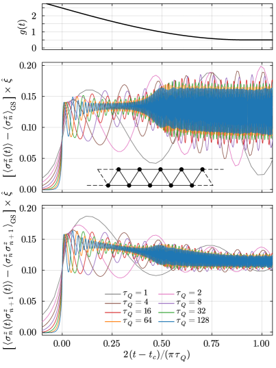
Figure 1: Oscillations during KZ ramp. Top: the KZ ramp crossing the critical point at $g_{c}=2.47725$ to end in the ferromagnetic phase at non-zero $g=0.5$. Middle: Rescaled transverse magnetization $\langle\sigma^{x}_{n}\rangle-\langle\sigma^{x}_{n}\rangle_{GS}$ during the ramp as a function of time, where $\langle\sigma^{x}_{n}\rangle_{GS}$ is its value in the adiabatic ground state and $\hat{\xi}=\sqrt{\tau_{Q}}$ is the KZ length. Its oscillation amplitude suddenly increases in the middle of the ferromagnetic phase. The inset shows the zigzag ladder. Bottom: NN ferromagnetic interaction energy as a function of time.

In Ref. 1, two models were studied. The simplest quantum Ising chain with only nearest-neighbor (NN) couplings is integrable and a paradigmatic example of quantum phase transitions. The Ising chain with both NN and next to NN (NNN) couplings is nonintegrable:

$$H=-\sum_{n=1}^{L}\left(g\sigma^{x}_{n}+\sigma^{z}_{n}\sigma^{z}_{n+1}+J_{2}\sigma^{z}_{n}\sigma^{z}_{n+2}\right).$$ (1)

Here, $\sigma_{n}^{x,y,z}$ are the Pauli operators on site $n$, $g$ is a transverse field, and $J_{2}$ is the NNN ferromagnetic coupling. It can be implemented with only NN couplings on a zigzag ladder in Fig. 1. Both models belong to the same universality class, so their behavior in the immediate vicinity of the critical point is expected to be essentially the same. Indeed, we have demonstrated  [1] that both models exhibit similar oscillatory behavior with KZM scalings following the quench.

Dramatic differences in the behavior between the two Ising chains arise away from the transition point. In the integrable quantum Ising chain with only NN couplings, post-critical coherent oscillations gradually decay. By contrast (and to our surprise), in the nonintegrable Ising chain with both NN and NNN couplings, the post-KZM oscillation decays, but before it disappears, it becomes enhanced and gives rise to persistent oscillation that does not decay on the timescales explored by our numerical simulations. These reincarnated oscillations have features that are no longer subject to KZM scalings (see Fig. 1). In particular, the frequencies of such oscillations are no longer controlled by the size of the Ising chain gap associated with a single quasiparticle.

The aim of this paper is to investigate properties and to characterize the nature of these oscillations.

Integrable NN chain; $\mathbf{J_{2}=0}$. We linearly ramp the transverse field  [50, 52, 58, 102, 86, 87] as

$$g(t)=g_{c}\left[1-\epsilon(t)\right]=g_{c}-g_{c}(t-t_{c})/\tau_{Q},$$ (2)

from a strong field at $t=-\infty$, across the critical point at $g(t_{c})=g_{c}=1$, to $g(t_{s})=0$ when the transverse field vanishes and the ramp stops. The Jordan-Wigner transformation maps the model to a set of independent Landau-Zener systems that can be solved analytically. In particular, the final density of excited quasiparticles/kinks scales like [50, 52, 103]

$$\rho=\frac{1}{2\pi\sqrt{2\tau_{Q}}}\propto\hat{\xi}^{-1}.$$ (3)

Here, $\hat{\xi}$ is the KZ length. The KZM operates within $\pm\hat{t}$ of $t_{c}$, where $\hat{t}\propto\hat{\xi}^{1}$. Prior to the kink count, the final state is a quantum superposition of different numbers [58, 73] and correlated locations of kinks [84, 86, 87] that manifests in coherent oscillations of the transverse magnetization $\sigma^{x}$ [1].

Two new results [103] make observation of the coherent oscillations more feasible for the present quantum simulation platforms. The first is an analytical formula for the transverse magnetization after $t_{c}+\hat{t}$:

$$\delta^{x}=\langle\sigma^{x}\rangle-\langle\sigma^{x}\rangle_{\rm GS}\approx 2\rho+\rho^{2}d\frac{57\sqrt{6\pi}}{80}\cos\phi.$$ (4)

Here, $d=(1+f^{2})^{-3/4}$ is a dephasing factor, where

$$f=\frac{3}{4\pi}\left[\gamma_{E}-2\frac{t-t_{c}}{\tau_{Q}}+\ln\frac{4(t-t_{c})^{2}}{\tau_{Q}}\right]$$ (5)

with Euler’s constant $\gamma_{E}$, the phase of the oscillations is

$$\phi=\frac{\pi}{4}+2\frac{(t-t_{c})^{2}}{\tau_{Q}}+\frac{3}{2}\arctan f,$$ (6)

and $\langle\sigma^{x}\rangle_{\rm GS}$ is the magnetization in the adiabatic ground state. In (4) both terms are accurate to their leading order in $\rho$. The second result is the NN ferromagnetic correlator:

$$\delta^{zz} = \langle\sigma^{z}_{n}\sigma^{z}_{n+1}\rangle-\langle\sigma^{z}_{n}\sigma^{z}_{n+1}\rangle_{\rm GS}$$ (7)

$$\approx -2\rho-g\leavevmode\nobreak\ \rho^{2}d\frac{57\sqrt{6\pi}}{80}\cos\phi,$$

which may be more directly accessible in some quantum simulation platforms. Together with (4), it satisfies $-\delta^{zz}-g\delta^{x}\approx 2(1-g)\rho.$ The excitation energy density on the left-hand side is given by the density of quasiparticles $\rho$ times the quasiparticle gap opening with the distance from the critical point as $2(1-g)$, in consistency with the extended QKZM [85].

The oscillations (4) are damped by dephasing of non-interacting quasiparticles. Breaking the integrability with $J_{2}=1$, one might expect them to become even more scrambled, but it turns out to be the other way around. Not only do they become more persistent, but even their amplitude is enhanced (see Fig. 1).

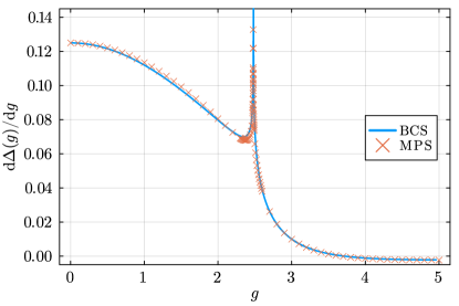
Figure 2: BCS versus MPS. The first derivative of the gap function $\Delta$ with respect to the field $g$ in the ground state from the BCS theory and matrix product states (MPS). Estimates of $g_{c}$ from BCS and MPS are $g_{c}=2.48135$ and $g_{c}=2.47725$, respectively.

Nonintegrable chain with $\mathbf{J_{2}=1}$; Kink pairs. With a fermionic operator that annihilates a kink on a bond between sites $n$ and $n+1$ [87],

$$f_{n}=\left(\prod_{l\leq n}\sigma^{x}_{l}\right)\frac{\sigma^{z}_{n}-\sigma^{z}_{n+1}}{2i},$$ (8)

one can rewrite the Hamiltonian (1) with $J_{2}=1$ as

$$H = -2L+6\sum_{n}f_{n}^{\dagger}f_{n}-4\sum_{n}f_{n}^{\dagger}f_{n}f_{n+1}^{\dagger}f_{n+1}$$ (9)

$$-g\sum_{n}\left(f_{n}^{\dagger}f_{n+1}+f_{n+1}f_{n}+{\rm h.c.}\right).$$

The first term is the energy of the ferromagnetic state and the second is that of individual kinks in this state. The transverse field in the second line can create/annihilate a pair of kinks on NN bonds by flipping the spin between them. A spin flip can also make a kink hop between NN bonds. The integrability is broken by the quartic attraction between NN kinks.

In the BCS theory, the ground state is assumed to be a fermionic Gaussian state $\ket{0}$. After a Fourier transform

$$f_{n}=e^{i\pi/4}\sum_{k}\frac{e^{ik(n+1/2)}}{\sqrt{L}}f_{k},$$ (10)

and a Bogoliubov transformation,

$$f_{k}=u_{k}\gamma_{k}+v_{-k}^{*}\gamma_{-k}^{\dagger},$$ (11)

the energy is minimized by a vacuum, $\gamma_{k}\ket{0}=0,$ where $(u_{k},v_{k})$ solve the Bogoliubov-de Gennes equations:

$$\omega_{k}\left(\begin{array}[]{c}u_{k}\\ v_{k}\end{array}\right)=\left(\begin{array}[]{cc}H_{k}&D_{k}\\ D^{*}_{k}&-H_{k}\end{array}\right)\left(\begin{array}[]{c}u_{k}\\ v_{k}\end{array}\right).$$ (12)

Here, $H_{k}=2(3-4\rho)-2(g-4t_{f})\cos k$, $D_{k}=-2(g+4\Delta)\sin k$, and the quasiparticle dispersion $\omega_{k}=\sqrt{H_{k}^{2}+D_{k}^{2}}$. Here, $\rho=\bra{0}f_{n}^{\dagger}f_{n}\ket{0}$ is density of kinks, $\Delta=\bra{0}f_{n+1}f_{n}\ket{0}$ is their anomalous density, and $t_{f}=\bra{0}f_{n+1}^{\dagger}f_{n}\ket{0}$ is a correction to the kink hopping rate. The BCS solution compares well with the matrix product states (MPS) [104] (see Fig. 2 and [103]). The critical $g_{c}=2.48135$ by BCS lies within $0.2\%$ of $g_{c}=2.47725$ by MPS VUMPS algorithm.

The accuracy of the BCS theory makes it a reliable approximation for the ground state. For $g\ll g_{c}$ it yields:

$$\rho=\frac{g^{2}}{32}+{\cal O}(g^{4}),\leavevmode\nobreak\ \leavevmode\nobreak\ \Delta=\frac{g}{8}+{\cal O}(g^{3}),\leavevmode\nobreak\ \leavevmode\nobreak\ t_{f}={\cal O}(g^{3}),$$ (13)

and the Bogoliubov coefficients:

$$u_{k} \approx \left(1-\frac{g^{2}}{64}\right)+\frac{g^{2}}{64}\cos 2k+{\cal O}(g^{3}),\leavevmode\nobreak\ \leavevmode\nobreak\$$

$$v_{k} \approx -\frac{g}{4}\sin k-\frac{g^{2}}{24}\sin 2k+{\cal O}(g^{3}).$$ (14)

With (11), we obtain the kink operator

$$f_{n} \approx \left(1-\frac{g^{2}}{64}\right)\gamma_{n}+\frac{g^{2}}{128}\left(\gamma_{n+2}+\gamma_{n-2}\right)$$ (15)

$$+\frac{g}{8}\left(\gamma_{n+1}^{\dagger}-\gamma_{n-1}^{\dagger}\right)+\frac{g^{2}}{48}\left(\gamma_{n+2}^{\dagger}-\gamma_{n-2}^{\dagger}\right).$$

Here, the position representation $\gamma_{n}$ is the transform (10) of $\gamma_{k}$. It is a kink $f_{n}$ dressed with quantum fluctuations. Beyond BCS, the exact Hamiltonian (9) becomes

$$H=E_{0}+\sum_{k}\omega_{k}\gamma_{k}^{\dagger}\gamma_{k}-4\sum_{n}:f_{n}^{\dagger}f_{n}f_{n+1}^{\dagger}f_{n+1}:.$$ (16)

Here, $E_{0}=\bra{0}H\ket{0}$, the normal ordering is with respect to $\gamma$, and the quasiparticle dispersion is

$$\omega_{k} = \omega_{\gamma}-2t_{\gamma}\cos k-2t^{\prime}_{\gamma}\cos 2k+{\cal O}(g^{3}),$$ (17)

where $\omega_{\gamma}=6+g^{2}/8$, $t_{\gamma}=g$ and $t^{\prime}_{\gamma}=3g^{2}/16$. With (15) the Hamiltonian (16) becomes

$$H = E_{0}+\omega_{\gamma}\sum_{n}\gamma_{n}^{\dagger}\gamma_{n}-\left(4-\frac{g^{2}}{8}\right)\sum_{n}\gamma_{n}^{\dagger}\gamma_{n+1}^{\dagger}\gamma_{n+1}\gamma_{n}$$ (18)

$$-t_{\gamma}\sum_{n}\left(\gamma_{n}^{\dagger}\gamma_{n+1}+{\rm h.c.}\right)+\frac{g}{2}\sum_{n}V_{n}^{(1)}$$

$$-t^{\prime}_{\gamma}\sum_{n}\left(\gamma_{n}^{\dagger}\gamma_{n+2}+{\rm h.c.}\right)+\frac{g^{2}}{16}\sum_{n}V^{(2)}_{n}$$

$$+g^{2}\tilde{V}^{(2)}+{\cal O}(g^{3}),$$

where

$$V_{n}^{(1)} = \left(\gamma_{n+2}^{\dagger}\gamma_{n+1}^{\dagger}+\gamma_{n-1}^{\dagger}\gamma_{n-2}^{\dagger}\right)\gamma_{n}^{\dagger}\gamma_{n}+{\rm h.c.},$$ (19)

$$V_{n}^{(2)} = \left(\gamma^{\dagger}_{n+1}\gamma^{\dagger}_{n}+\gamma^{\dagger}_{n+2}\gamma^{\dagger}_{n+1}\right)\gamma_{n}\gamma_{n-1}+{\rm h.c.},$$ (20)

and $\tilde{V}^{(2)}$ collects remaining terms that do not contribute to (21) [103]. For $g\ll g_{c}$, the first line of (18) dominates, and pairs of NN quasiparticles form tight bound states. These are single reversed spins dressed in quantum fluctuations.

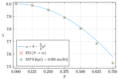
Figure 3: Oscillation frequency. The plot compares (22) with the gap between the ground and first excited state obtained with exact diagonalization (ED) extrapolated to infinite periodic chain size ($L\to\infty$), and transverse oscillation frequency after the periodic drive (24) with small amplitude obtained by a fit to MPS simulations. The ED and MPS error bars are on the order of the marker stroke width.

Accordingly, we introduce NN pair operators $b_{n}=\gamma_{n+1}\gamma_{n}$. They are approximately bosonic at low pair density where an effective Hamiltonian can be obtained as [103]

$$H_{b} = \omega_{b}\sum_{n}b_{n}^{\dagger}b_{n}-t_{b}\sum_{n}\left(b^{\dagger}_{n}b_{n+1}+{\rm h.c.}\right)$$ (21)

$$-t^{\prime}_{b}\sum_{n}\left(b^{\dagger}_{n}b_{n+2}+{\rm h.c.}\right)+{\cal O}\left(g^{3}\right).$$

Here, $\omega_{b}=8-g^{2}/4$, $t_{b}=g^{2}/8$, and $t^{\prime}_{b}=g^{2}/8$. A pair has minimal energy for zero pair quasimomentum:

$$\omega=\omega_{b}-2t_{b}-2t^{\prime}_{b}=8-\frac{3}{4}g^{2},$$ (22)

which agrees with the gap from exact diagonalization in Fig. 3.

Within a dynamic BCS theory, the KZ ramp results in a fermionic Gaussian state where pairs of $\gamma$-quasiparticles are not bound but free to move along the chain [87]. Bound pairs would not affect the long-range order, while the actual state has finite ferromagnetic domains of typical size $\hat{\xi}$. The free quasiparticles occupy quasimomenta up to $\propto\hat{\xi}^{-1}$, and their non-trivial dispersion makes dephasing inevitable.

However, as $g$ is slowly ramped further down, the individual $\gamma$-quasiparticles become unstable towards the lower energy branch of pair excitations. This happens when the pair gap in (22) becomes lower than twice the $\gamma$-gap in (17), $\omega<2\omega_{0}$, near $g_{0}\approx 1.12$ (see Fig. 4). The pair dispersion is weaker than the dispersion of $\gamma$-quasiparticles ($\propto g^{2}$ in (21) versus $\propto g$ in (17), respectively) but not weak enough to explain the absence of dephasing that we observe for times much longer than $\propto g^{-2}$. It is made irrelevant by a Bose-enhanced transfer of $\gamma$-quasiparticles into pairs with zero quasimomentum. The appearance of pairs manifests in Fig. 1 by the amplification of oscillations near $g_{0}$, as can be explained with a simple example: for $\ket{\psi}=\alpha\ket{0}+\beta b_{n-1}^{\dagger}\ket{0}e^{-i\omega t}$ we obtain

$$\bra{\psi}\sigma^{x}_{n}\ket{\psi}\approx$$

$$\bra{\psi}\gamma_{n-1}^{\dagger}\gamma_{n}+\gamma_{n}^{\dagger}\gamma_{n-1}-\gamma_{n-1}\gamma_{n}-\gamma_{n}^{\dagger}\gamma_{n-1}^{\dagger}\ket{\psi}=$$

$$\alpha^{*}\beta e^{-i\omega t}+\alpha\beta^{*}e^{+i\omega t}.$$ (23)

As the pair is a reversed $n$-th spin (dressed in quantum fluctuations), it manifests in oscillations of the spin-reversing $\sigma^{x}_{n}$.

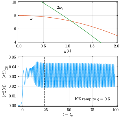
Figure 4: Oscillations after KZ ramp. Top: the energy gap for creating a pair of fermionic quasiparticles, $2\omega_{0}$, versus that for their bound pair, $\omega$. They crossover near $g_{0}=1.12$. Bottom: oscillations after a smooth KZ ramp to $g=0.5$ with $\tau_{Q}=16$, using a smooth ramp $g(t)=g_{c}[2-(1-0.5/(2g_{c}))(1+\sin(t/\tau_{Q}))],t\in[-\tau_{Q}\times\pi/2,\tau_{Q}\times\pi/2]$. The dashed line indicates the end of the ramp, followed by a free evolution at $g=0.5$. The oscillations during the free evolution have a Q factor of ${\approx}4012$ for $\tau_{Q}=16$, which increases to $Q\approx 8000$ for $\tau_{Q}=32$.

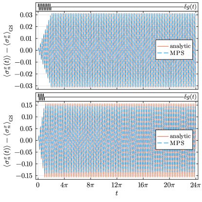
Figure 5: Periodic driving. Top: coherent transverse field oscillations at $g=0.25$ after driving $\delta g(t)=0.005\sin(8t)$ close to resonance for time $2\pi$. The plot compares (28) with MPS simulations. The maximum percentage difference between (28) and MPS simulations is less than $0.8\%$. Bottom: the same at $g=0.5$ after driving $\delta g(t)=0.05\sin(8t)$ for time $\pi$. The Q factors of the top and bottom plots are $Q\approx 461504$ and $Q\approx 8307$, respectively.

Periodic drive. The KZ ramp is not the most efficient way to excite coherent oscillations. Starting from a ground state at $g$, the pair condensate can also be readily excited by a time-dependent perturbation to the Hamiltonian

$$\delta H=\delta g(t)\sum_{n}\sigma^{x}_{n}.$$ (24)

Assuming a small density of pairs, where their hard-core nature can be ignored and there is a gap between paired and unpaired quasiparticles ($g\ll g_{0}$), we can approximate the transverse magnetization as

$$\sum_{n}\left(\sigma^{x}_{n}-\langle\sigma^{x}_{n}\rangle_{GS}\right)\approx\sum_{n}\left(b_{n}+b_{n}^{\dagger}\right)=\sqrt{L}\left(\tilde{b}_{0}+\tilde{b}_{0}^{\dagger}\right),$$ (25)

where $\tilde{b}_{k}=e^{i\pi/4}b_{k}$, and the pair Hamiltonian (21) becomes

$$H^{\prime}_{b} = \sum_{k}\omega_{b,k}\tilde{b}_{k}^{\dagger}\tilde{b}_{k}+\delta H.$$ (26)

Here, $\omega_{b,k}=\omega_{b}-2t_{b}\cos k-2t^{\prime}_{b}\cos 2k$. Since only $k=0$ is driven by $\delta H$ in (25), it reduces to a driven oscillator:

$$H^{\prime}_{\rm b,0} = \omega\tilde{b}_{0}^{\dagger}\tilde{b}_{0}+\delta g(t)\sqrt{L}\left(\tilde{b}_{0}+\tilde{b}_{0}^{\dagger}\right).$$ (27)

The driving generates a coherent state of $\tilde{b}_{0}$ bosons. Starting from the ground state, the transverse magnetization evolves as

$$\left(\frac{d^{2}}{dt^{2}}+\omega^{2}\right)\left(\langle\sigma^{x}_{n}\rangle-\langle\sigma^{x}_{n}\rangle_{GS}\right)=-2\omega\leavevmode\nobreak\ \delta g(t).$$ (28)

The pairs manifest themselves also in the correlators:

$$-\sum_{n}\langle\sigma^{z}_{n}\sigma^{z}_{n+1}\rangle\approx-\sum_{n}\langle\sigma^{z}_{n}\sigma^{z}_{n+2}\rangle\approx$$

$$\leavevmode\nobreak\ \leavevmode\nobreak\ \leavevmode\nobreak\ \leavevmode\nobreak\ \leavevmode\nobreak\ \leavevmode\nobreak\ \leavevmode\nobreak\ \leavevmode\nobreak\ \leavevmode\nobreak\ \leavevmode\nobreak\ -L+4\sum_{n}\langle b_{n}^{\dagger}b_{n}\rangle+\frac{g}{2}\sqrt{L}\left\langle\tilde{b}_{0}+\tilde{b}_{0}^{\dagger}\right\rangle.$$ (29)

A weak driving for a finite time results in persistent oscillations with a well-defined frequency. Fig. 5 shows their examples for $g=0.25,0.5$. Fig. 3 demonstrates the frequency to be consistent with the gap estimate from exact diagonalization and the perturbative formula (22).

Conclusion. In the NN and NNN quantum Ising chain (or the NN zigzag ladder), the fermionic Bogoliubov quasiparticles below the critical transverse magnetic field give way to their tightly bound Cooper pairs as the lowest branch of excitations. They can be readily excited by the KZ ramp or periodic driving. Despite nonintegrability, the excitation manifests by persistent coherent oscillations contributing an example to a variety of phenomena like quantum many-body scars [105, 106, 107, 108] or quantum time crystals [109].

Acknowledgements. This research was funded by the National Science Centre (NCN), Poland, under project 2021/03/Y/ST2/00184 within the QuantERA II Programme that has received funding from the European Union’s Horizon 2020 research and innovation programme under Grant Agreement No 101017733 (FB), NCN under projects 2019/35/B/ST3/01028 (JD) and 2020/38/E/ST3/00150 (MMR) , and Department of Energy under the Los Alamos National Laboratory LDRD Program (WHZ). The research was also supported by a grant from the Priority Research Area DigiWorld under the Strategic Programme Excellence Initiative at Jagiellonian University (JD, MMR).

The supplementary material can be divided into two parts. The first one, from App. A to App. C, outlines the complete solution of the integrable NN quantum Ising chain that naturally leads to the new results presented in the main text. The standard parts of the solution are based on four papers: two older items [52, 59] and two more recent ones [86, 87, 1]. They are included here to make the supplementary material self-contained. App. B derives oscillations between $t_{c}+\hat{t}$ and the end of the ramp and App. C estimates their dephasing rate and the quality factor. The second part, from D to G, deals with the nonintegrable chain.

Both the first part and the BCS theory in App. D use a fermionic Bogoliubov theory. The two theories are not the same and should not be confused even though we use the same symbols like $u_{k},v_{k}$. The former is in the representation of Jordan-Wigner fermions, while the latter is in that of kinks.

Appendix A Quantum Ising chain

The Hamiltonian for transverse field quantum Ising chain reads

$$H\leavevmode\nobreak\ =\leavevmode\nobreak\ -\sum_{n=1}^{L}\left(\sigma^{z}_{n}\sigma^{z}_{n+1}+g\sigma^{x}_{n}\right)\leavevmode\nobreak\ ,$$ (S1)

where we consider a system of $L$ spins one-half with periodic boundary conditions, $\vec{\sigma}_{L+1}\leavevmode\nobreak\ =\leavevmode\nobreak\ \vec{\sigma}_{1}$. In the limit of $L\to\infty$, there are quantum critical points at $g_{c}=\pm 1$, respectively, that separate the paramagnetic phase for $|g|>1$ from the ferromagnetic phase for $|g|$<1. For simplicity of presentation, we additionally assume that $L$ is even. The Jordan-Wigner transformation,

$$\sigma^{x}_{n}\leavevmode\nobreak\ =\leavevmode\nobreak\ 1-2c^{\dagger}_{n}c_{n}\leavevmode\nobreak\ ,$$ (S2)

$$\sigma^{z}_{n}\leavevmode\nobreak\ =\leavevmode\nobreak\ -\left(c_{n}+c_{n}^{\dagger}\right)\prod_{m<n}(1-2c^{\dagger}_{m}c_{m})\leavevmode\nobreak\ ,$$ (S3)

introduces fermionic annihilation ($c_{n}$) and creation ($c^{\dagger}_{n}$) operators. It maps the Hamiltonian in Eq. (S1) to

$$H\leavevmode\nobreak\ =\leavevmode\nobreak\ P^{+}\leavevmode\nobreak\ H^{+}\leavevmode\nobreak\ P^{+}\leavevmode\nobreak\ +\leavevmode\nobreak\ P^{-}\leavevmode\nobreak\ H^{-}\leavevmode\nobreak\ P^{-}\leavevmode\nobreak\ .$$ (S4)

The projectors on subspaces with even ($+$) and odd ($-$) numbers of $c$-quasiparticles read

$$P^{\pm}=\frac{1}{2}\left[1\pm\prod_{n=1}^{L}\sigma^{x}_{n}\right]=\frac{1}{2}\left[1\leavevmode\nobreak\ \pm\leavevmode\nobreak\ \prod_{n=1}^{L}\left(1-2c_{n}^{\dagger}c_{n}\right)\right].$$ (S5)

The reduced Hamiltonians in each parity subspace,

$$H^{\pm}\leavevmode\nobreak\ =\leavevmode\nobreak\ \sum_{n=1}^{L}\left[g\left(c_{n}^{\dagger}c_{n}-\frac{1}{2}\right)-c_{n}^{\dagger}c_{n+1}+c_{n}c_{n+1}\right]+{\rm h.c.},$$ (S6)

differ in boundary conditions. Namely, in $H^{-}$ we assume periodic boundary conditions, $c_{L+1}=c_{1}$, and in $H^{+}$ we have antiperiodic boundary conditions, $c_{L+1}=-c_{1}$.

The parity of the number of $c$-quasiparticles commutes with the Hamiltonian. As the ground state for $g\gg 1$ has even parity, we limit ourselves to that relevant subspace. The next step in the diagonalization of $H^{+}$ is a Fourier transform,

$$c_{n}\leavevmode\nobreak\ =\leavevmode\nobreak\ \frac{e^{-i\pi/4}}{\sqrt{L}}\sum_{k}c_{k}e^{ikn}\leavevmode\nobreak\ ,$$ (S7)

with half-integer pseudo-momenta consistent with the antiperiodic boundary conditions,

$$k\leavevmode\nobreak\ =\leavevmode\nobreak\ \pm\frac{1}{2}\frac{2\pi}{L},\pm\frac{3}{2}\frac{2\pi}{L},\dots,\pm\frac{L-1}{2}\frac{2\pi}{L}\leavevmode\nobreak\ .$$ (S8)

After this transformation, the Hamiltonian takes the form

$$H^{+}\leavevmode\nobreak\ = \sum_{k} \left[(g-\cos k)\left(c_{k}^{\dagger}c_{k}-c_{-k}c_{-k}^{\dagger}\right)+\right.$$ (S9)

$$\left.\leavevmode\nobreak\ \leavevmode\nobreak\ \sin k\left(c^{\dagger}_{k}c^{\dagger}_{-k}+c_{-k}c_{k}\right)\right]\leavevmode\nobreak\ .$$

Its diagonalization is completed by a Bogoliubov transformation,

$$c_{k}\leavevmode\nobreak\ =\leavevmode\nobreak\ u_{k}\gamma_{k}+v_{-k}^{*}\gamma^{\dagger}_{-k}\leavevmode\nobreak\ ,$$ (S10)

where the Bogoliubov modes $(u_{k},v_{k})$ follow as eigenstates of the Bogoliubov-de Gennes equations,

$$\epsilon\leavevmode\nobreak\ u_{k} = +2(g-\cos k)u_{k}+2\sin k\leavevmode\nobreak\ v_{k},$$

$$\epsilon\leavevmode\nobreak\ v_{k} = -2(g-\cos k)v_{k}+2\sin k\leavevmode\nobreak\ u_{k}.$$ (S11)

There are two eigenstates for each value of $k$, with eigenfrequencies $\epsilon=\pm\epsilon_{k}$,

$$\epsilon_{k}\leavevmode\nobreak\ =\leavevmode\nobreak\ 2\sqrt{(g-\cos k)^{2}+\sin^{2}k}\leavevmode\nobreak\ .$$ (S12)

The eigenstates with positive frequency, $(u^{+}_{k},v^{+}_{k})=(\cos(\theta_{k}/2),\sin(\theta_{k}/2))$, define a fermionic quasiparticle operator $\gamma_{k}\leavevmode\nobreak\ =\leavevmode\nobreak\ u_{k}^{+*}c_{k}+v^{+}_{-k}c_{-k}^{\dagger}$, where angles $\theta_{k}$ satisfy $(\cos\theta_{k},\sin\theta_{k})=\frac{2}{\epsilon_{k}}(g-\cos k,\sin k)$. The negative frequency ones, with $(u^{-}_{k},v^{-}_{k})=(v^{+}_{k},-u^{+}_{k})$, formally define $\gamma_{k}^{-}=u_{k}^{-*}c_{k}+v_{-k}^{-}c_{-k}^{\dagger}=-\gamma_{-k}^{\dagger}$. After the Bogoliubov transformation, the Hamiltonian reads

$$H^{+}\leavevmode\nobreak\ =\leavevmode\nobreak\ \sum_{k}\epsilon_{k}\leavevmode\nobreak\ \left(\gamma_{k}^{\dagger}\gamma_{k}\leavevmode\nobreak\ -\frac{1}{2}\right).$$ (S13)

Note that, due to the projector $P^{+}$ in Eq. (S4), only states with even numbers of $c$-quasiparticles belong to the spectrum of $H$.

The quasiparticle dispersion in Eq. (S12) implies a linear dispersion for small $k$ at the critical $g=1$, $\epsilon_{k}\approx 2|k|$, and the dynamical exponent $z$ is equal to $1$. Moreover, for $k=0$, we have $\epsilon_{0}\propto|g-1|^{1}$ and $z\nu=1$. Finally, the correlation length exponent $\nu$ is equal to $1$.

Appendix B Linear quench and the Landau-Zener problem

The Hamiltonian follows a linear ramp in the transverse field,

$$g(t\leq 0)\leavevmode\nobreak\ =\leavevmode\nobreak\ -\frac{t}{\tau_{Q}},$$ (S14)

with the quench rate $\tau_{Q}$. For convenience, here we fix the time when the ramp reaches $g(t_{s})=0$ at $t_{s}=0$ (we use $t_{s}$ in the main text for clarity). As such, time $t$ runs from $-\infty$ to $0$ when the ramp stops at transverse field $g=0$, crossing the critical point at $g_{c}=1$ when $t_{c}=-\tau_{Q}$. The system starts in the ground state at $g\to\infty$, where $(u_{k},v_{k})=(1,0)$, and is the vacuum state annihilated by all corresponding Bogoliubov operators, $\gamma_{k}|0\rangle=0$.

In addressing the dynamical problem, it is convenient to employ the Heisenberg picture. The state of the system stays as the vacuum of Bogoliubov operators $\gamma_{k}$, while the Bogoliubov modes evolve according to the Heisenberg equation of motion $i\frac{d}{dt}c_{k}=[c_{k},H^{+}]$. Following the time-dependent Bogoliubov transformation,

$$c_{k}=u_{k}(t)\gamma_{k}+v_{-k}^{*}(t)\gamma^{\dagger}_{-k},$$ (S15)

this gives time-dependent Bogoliubov-de Gennes equations,

$$i\frac{d}{dt}u_{k} = +2\left(g(t)-\cos k\right)u_{k}+2\sin k\leavevmode\nobreak\ v_{k}\leavevmode\nobreak\ ,$$

$$i\frac{d}{dt}v_{k} = -2\left(g(t)-\cos k\right)v_{k}+2\sin k\leavevmode\nobreak\ u_{k}\leavevmode\nobreak\ ,$$ (S16)

and the initial condition is $(u_{k}(-\infty),v_{k}(-\infty))=(1,0)$.

Introducing a new time variable,

$$\tau\leavevmode\nobreak\ =\leavevmode\nobreak\ 4\tau_{Q}\sin k\left(\frac{t}{\tau_{Q}}+\cos k\right),$$ (S17)

that runs from $-\infty$ to $\tau^{\rm final}_{k}=2\tau_{Q}\sin(2k)$ for $t=0$, allows one to map Eq. (S16) to the Landau-Zener (LZ) problem [52, 59],

$$i\frac{d}{d\tau}u_{k} = -\frac{1}{2}\tau\Delta_{k}\leavevmode\nobreak\ u_{k}+\frac{1}{2}v_{k},$$

$$i\frac{d}{d\tau}v_{k} = +\frac{1}{2}\tau\Delta_{k}\leavevmode\nobreak\ v_{k}+\frac{1}{2}u_{k}.$$ (S18)

Here, $\Delta_{k}=(4\tau_{Q}\sin^{2}k)^{-1}$ sets an efficient rate of the transition for given $k$.

Only modes with small $k$ that have small energy gaps at their anti-crossing point can get excited when the ramp is slow. For such modes, $\tau^{\rm final}_{k}$ is much longer than the time when the anti-crossing is completed and we are allowed to use the LZ formula,

$$p_{k}\leavevmode\nobreak\ \approx\leavevmode\nobreak\ e^{-\frac{\pi}{2\Delta_{k}}}\leavevmode\nobreak\ \approx\leavevmode\nobreak\ e^{-2\pi\tau_{Q}k^{2}}\leavevmode\nobreak\ ,$$ (S19)

where approximations become accurate for $\tau_{Q}\gg 1$. Eq. (S19) gives the probability that a pair of quasiparticles with quasimomenta $+k$ and $-k$ got excited. The mean density of kinks at $g=0$ is simply given by $\rho=\sum_{k}p_{k}/L$ [52]. Taking the limit $L\to\infty$,

$$\rho=\lim_{L\to\infty}\frac{1}{L}\sum_{k}p_{k}=\frac{1}{2\pi}\int_{-\pi}^{\pi}dk\leavevmode\nobreak\ p_{k}\approx\frac{1}{2\pi\sqrt{2\tau_{Q}}}.$$ (S20)

The density scales as an inverse of $\hat{\xi}\propto\tau_{Q}^{1/2}$, in full consistency with KZM prediction for $\nu=z=1$. For convenience, we can use the density of kinks to supplement the numerical prefactor

$$\hat{\xi}\equiv\frac{1}{\rho}=2\pi\sqrt{2\tau_{Q}},$$ (S21)

making its inverse equal to the mean density of kinks at the end of the ramp at $g=0$.

B.1 Ramp to zero transverse field

To characterize the oscillations, we require more than just the excitation spectrum in Eq. (S19). A general solution to Eqs. (S18) has the form [110, 59],

$$v_{k}(\tau) = -aD_{-s-1}(-iz)-bD_{-s-1}(iz),$$

$$u_{k}(\tau) = \left(-\Delta_{k}\tau+2i\frac{\partial}{\partial\tau}\right)v_{k}(\tau),$$ (S22)

where $D_{m}(x)$ is a Weber function, $s^{-1}=4i\Delta_{k}$, and $iz=\sqrt{\Delta_{k}}\tau e^{i\pi/4}$. Constants $a,b$ are fixed by initial conditions. From the asymptotic behavior of the Weber function when $\tau\to-\infty$, one gets $a=0$, and

$$|b|^{2}=\frac{e^{-\pi/8\Delta_{k}}}{4\Delta_{k}}\leavevmode\nobreak\ .$$ (S23)

On the other hand, at the end of the ramp when $t=0$ and $\tau=2\tau_{Q}\sin(2k)$ the argument of the Weber function reads $iz=2\sqrt{\tau_{Q}}e^{i\pi/4}{\rm sign}(k)\cos(k)$. Its absolute value is large for slow transitions (except near $k=\pm\frac{\pi}{2}$), and one can again use the asymptotic behavior of the Weber function  [59].

When $(t-t_{c})\gg\hat{t}$ the evolution becomes adiabatic and the time-dependent Bogoliubov modes can be accurately decomposed as

$$\left(\begin{array}[]{c}u_{k}\\ v_{k}\end{array}\right)=\sqrt{1-p_{k}}\left(\begin{array}[]{c}u^{+}_{k}\\ v^{+}_{k}\end{array}\right)+\sqrt{p_{k}}\left(\begin{array}[]{c}v^{+}_{k}\\ -u^{+}_{k}\end{array}\right)e^{i\varphi_{k}(t)},$$ (S24)

were $(u^{+}_{k},v^{+}_{k})$ is a positive-frequency stationary Bogoliubov mode at $g(t)$. With the asymptotic behavior of the Weber function the phase at $t=0$ reads [59]:

$$\varphi_{k}(0) = \frac{\pi}{4}+2\tau_{Q}-(2-\ln 4)k^{2}\tau_{Q}+k^{2}\tau_{Q}\ln\tau_{Q}+$$ (S25)

$$- \arg\left[\Gamma\left(1+ik^{2}\tau_{Q}\right)\right]\leavevmode\nobreak\ .$$

Above, $\varphi_{k}$ is a dynamical phase acquired by a pair of excited quasiparticles $(k,-k)$, with $\Gamma(x)$ being the gamma function. We follow [86], and approximate ${\rm arg}[\Gamma\left(1+i\tau_{Q}k^{2}\right)]\approx-\gamma_{E}\tau_{Q}k^{2}$ to make the phase more tractable. Here $\gamma_{E}$ is the Euler gamma constant. The approximation is valid for small enough $\tau_{Q}k^{2}$, which is consistent with the fact that excited quasiparticles have at most $\tau_{Q}k^{2}\approx 1/2\pi$, see Eq. (S19). This makes $\varphi_{k}$ conveniently quadratic in $k$,

$$\varphi_{k}(0)=\frac{\pi}{4}+2\tau_{Q}+\left(\ln\tau_{Q}+\ln 4-2+\gamma_{E}\right)k^{2}\tau_{Q}$$ (S26)

This formula completes the full characterization of the Bogoliubov modes when the linear ramp ends at $g=0$.

B.2 Ramp after $\mathbf{+\hat{t}}$

In order to obtain phase $\varphi_{k}(t)$ at earlier time $t<0$, we have to subtract from (S26) the dynamical phase acquired between $t$ and the final time when $g=0$. The dynamical phase depends on the spectrum of quasiparticles that for small $k$ can be approximated as

$$\epsilon_{k}(g)\approx 2(1-g)+\frac{g}{(1-g)}k^{2}.$$ (S27)

The dynamical phase at time $t$ can be obtained as

$$\varphi_{k}(t) = \varphi_{k}(0)-2\int_{t}^{0}dt^{\prime}\epsilon_{k}[g(t^{\prime})]$$

$$= \varphi_{k}(0)-2\int_{t}^{0}dt^{\prime}\left[2[1-g(t^{\prime})]+\frac{g(t^{\prime})}{[1-g(t^{\prime})]}k^{2}\right]$$

$$= \frac{\pi}{4}+\frac{2t_{+}^{2}}{\tau_{Q}}+\left(\gamma_{E}-\frac{2t_{+}}{\tau_{Q}}+\ln\frac{4t_{+}^{2}}{\tau_{Q}}\right)k^{2}\tau_{Q},$$

where $t_{+}=t-t_{c}$. This formula is valid for small $k$ within the support of $p_{k}$.

Within the same support we can approximate $u_{k}^{+}\approx k/2/(1-g)+{\cal O}(k^{3})$ and $v_{k}^{+}\approx 1+{\cal O}(k^{2})$. With this approximation relevant products of Bogoliubov modes that follow from (S24) become

$$|v_{k}|^{2} \approx |v_{k}^{+}|^{2}-p_{k}-\sqrt{p_{k}(1-p_{k})}\frac{k\cos\varphi_{k}(t)}{(1-g)}$$

$$u_{k}v_{k}^{*} \approx u_{k}^{+}v_{k}^{+}-p_{k}\frac{k}{(1-g)}+\sqrt{p_{k}(1-p_{k})}e^{i\varphi_{k}(t)}.$$

The last terms with $\varphi_{k}(t)$ — that contribute to oscillations — and the middle terms with $p_{k}$ are approximated by their leading terms in powers of $k$. They will become the leading terms in $\rho$.

In order to make the following integrals analytically tractable we approximate [86]:

$$\sqrt{p_{k}(1-p_{k})}\approx e^{-a\pi\tau_{Q}k^{2}}A\sqrt{2\pi}\left(\tau_{Q}k^{2}\right)^{1/2}.$$ (S29)

Here, $A$ and $a$ are variational parameters that can be optimally chosen as $A\approx 19/20$ and $a\approx 4/3$. The transverse field is

$$\langle\sigma^{x}_{n}\rangle=1-2\int_{0}^{\pi}\frac{dk}{\pi}\left|v_{k}\right|^{2}.$$ (S30)

The integration yields (4). The NN ferromagnetic correlator is

$$\langle\sigma^{z}_{n}\sigma^{z}_{n+1}\rangle=2\int_{0}^{\pi}\frac{dk}{\pi}\left|v_{k}\right|^{2}\cos k+2{\rm Re}\int_{0}^{\pi}\frac{dk}{\pi}u_{k}v_{k}^{*}\sin k.$$ (S31)

After approximating $\cos k\approx 1$ and $\sin k\approx k$ to leading order in $k$ and then performing the integral, we obtain (7) that is accurate to leading order in $\rho$. The other correlator is

$$\langle\sigma^{y}_{n}\sigma^{y}_{n+1}\rangle=2\int_{0}^{\pi}\frac{dk}{\pi}\left|v_{k}\right|^{2}\cos k-2{\rm Re}\int_{0}^{\pi}\frac{dk}{\pi}u_{k}v_{k}^{*}\sin k.$$ (S32)

With the same approximations, we obtain

$$\delta^{yy}=-2\rho-(2-g)\rho^{2}d\frac{57\sqrt{6\pi}}{80}\cos\phi.$$ (S33)

It does not vanish at $g=0$.

Appendix C Oscillations and dephasing after $\mathbf{+\hat{t}}$

The expansion in Eq. (S24) becomes accurate at times later than $\hat{t}$ after the phase transition. The phase $\varphi_{k}$ increases as

$$\varphi_{k}(t)=\int^{t}dt^{\prime}\leavevmode\nobreak\ 2\epsilon_{k}[g(t^{\prime})].$$ (S34)

After $\hat{t}$, the quasiparticle spectrum for KZM excitations that are localized near $k=0$ can be considered flat and equal to the gap $\epsilon_{0}(g)$ that opens with the increasing distance from the critical point. Therefore, the transverse field oscillates with frequency given by twice the instantaneous gap. With (S27)

$$T=\frac{2\pi}{2\epsilon_{0}(g)}=\frac{\pi}{2(1-g)}$$ (S35)

is the period of the oscillations.

Beyond the approximation of flat dispersion, there is some dephasing. The dephasing time can be estimated with the help of the approximate dispersion relation in Eq. (S27). The difference between $\epsilon_{k}$ for $\hat{k}\approx 1/\sqrt{\tau_{Q}}$ and $k=0$ is $\delta\epsilon\approx\frac{g}{|1-g|\tau_{Q}}$. Therefore, the phase gets scrambled on a timescale

$$\tau_{D}=\frac{\pi}{\delta\epsilon}\approx\frac{\pi|1-g|\tau_{Q}}{g}.$$ (S36)

When combined with the period (S35) it yields a quality factor:

$$Q=\frac{\tau_{D}}{T}\approx 2\tau_{Q}\frac{(1-g)^{2}}{g}.$$ (S37)

It diverges at $g=0$ when the dispersion is flat and is the smallest soon after $\hat{t}$ when $1-g\approx 1/\sqrt{\tau_{Q}}$ and $Q\approx 2$. For a later $g$ it improves with increasing $\tau_{Q}$ that makes the excitations more narrow in $k$ reducing the dispersion.

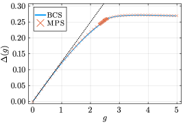
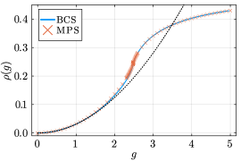
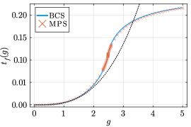
Figure S1: BCS versus MPS. Comparison between expectation values (from top to bottom) $\Delta$, $\rho$, and $t_{f}$ obtained within the BCS theory and with infinite matrix product states (MPS). The dotted lines are the perturbative formulas (13).

Appendix D BCS theory

By Wick’s theorem, the energy per site is

$$L^{-1}\bra{0}H\ket{0} = -(J_{1}+J_{2})+2\left(J_{1}+2J_{2}\right)\rho$$ (S38)

$$-g\left(t_{f}+t_{f}^{*}+\Delta+\Delta^{*}\right)$$

$$-4J_{2}\left(\rho^{2}+\Delta^{*}\Delta-t_{f}^{*}t_{f}\right).$$

It is energetically favorable we assume $\Delta$ and $t_{f}$ real. Self-consistency requires the expectation values to satisfy:

$$\rho = \int_{-\pi}^{\pi}\frac{dk}{2\pi}v_{k}^{2},$$ (S39)

$$t_{f} = \int_{-\pi}^{\pi}\frac{dk}{2\pi}v_{k}^{2}\cos k,$$ (S40)

$$\Delta = -\int_{-\pi}^{\pi}\frac{dk}{2\pi}u_{k}v_{k}\sin k.$$ (S41)

Here we used that $u_{k},v_{k}$ are real and have opposite parities with respect to $k$. A self-consistent solution of the Bogoliubov-de Gennes equations is shown in Fig. S1 where it is compared with results obtained with the matrix product states (MPS). Derivatives of the averages with respect to $g$ are shown in Fig. 2 in the main text and here in Fig. S2. The derivatives allow to locate the critical point at $g_{c}=2.48135$ (BCS) and $g_{c}=2.47725$ (MPS). These estimates agree within $0.2\%$.

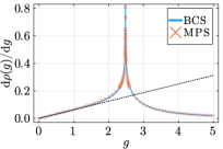
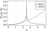
Figure S2: BCS versus MPS. First derivatives with respect to the field $g$ of $\rho$, and $t_{f}$ in the ground state from the BCS theory and matrix product states (MPS) in Fig. S1. A derivative of $\Delta$ is shown in Fig. 2 in the main text. Estimates of $g_{c}$ from BCS and MPS are $g_{c}=2.48135$ and $g_{c}=2.47725$, respectively. The dotted lines are the derivatives of the perturbative formulas (13).

Appendix E Effective pair Hamiltonian

The effective pair Hamiltonian (21) follows from the kink Hamiltonian in (18), (19), and (20). It operates in a Hilbert space spanned by Fock states

$$b_{n_{1}}^{\dagger}\dots b_{n_{M}}^{\dagger}|0\rangle,$$ (S42)

where $n_{i}+1<n_{i+1}$. From the second and third term in the first line of (18) we obtain a contribution to the pair energy $\omega_{b}$ in (21)

$$\omega_{b}^{(1)}=2\left(6+\frac{g^{2}}{8}\right)-\left(4-\frac{g^{2}}{8}\right)=8+\frac{3g^{2}}{8}.$$ (S43)

In terms of pair operators, the third line in (18) reads

$$t^{\prime}_{\gamma}\sum_{n}\left(b_{n}^{\dagger}b_{n+1}+{\rm h.c.}\right)+$$

$$-\frac{g^{2}}{16}\sum_{n}\left(b_{n}^{\dagger}b_{n-1}+b^{\dagger}_{n+1}b_{n-1}+{\rm h.c.}\right).$$ (S44)

Its contribution to the NN and NNN hopping terms in (21) are

$$t_{b}^{(1)} = -t^{\prime}_{\gamma}+\frac{g^{2}}{16}=-\frac{g^{2}}{8},$$ (S45)

$$t^{\prime(1)}_{b} = \frac{g^{2}}{16}.$$ (S46)

The second line of (18), which is linear in $g$, breaks/creates/annihilates pairs. Its contributions are second-order perturbative corrections to the pair energy and the NNN hopping. The $t_{\gamma}$-term contributes:

$$\omega^{(2)}_{b} = -2\frac{t_{\gamma}^{2}}{4}=-\frac{g^{2}}{2},$$ (S47)

$$t^{(2)}_{b} = \frac{t_{\gamma}^{2}}{4}=\frac{g^{2}}{4},$$ (S48)

and the $V^{(1)}$-terms contribute:

$$\omega^{(3)}_{b} = -2\frac{(g/2)^{2}}{4}=-\frac{g^{2}}{8},$$ (S49)

$$t^{\prime(3)}_{b} = \frac{(g/2)^{2}}{4}=\frac{g^{2}}{16}.$$ (S50)

Adding up all contributions, we obtain $\omega_{b}=\omega^{(1)}_{b}+\omega^{(2)}_{b}+\omega^{(3)}_{b}=8-g^{2}/4$, $t_{b}=t_{b}^{(1)}+t_{b}^{(2)}=g^{2}/8$, and $t^{\prime}_{b}=t^{\prime(1)}_{b}+t^{\prime(3)}_{b}=g^{2}/8$.

The second order term:

$$g^{2}\tilde{V}^{(2)} = \frac{g^{2}}{8}\sum_{n}\gamma_{n+1}^{\dagger}\gamma_{n-1}^{\dagger}\gamma_{n-1}\gamma_{n+1}+$$ (S51)

$$-\frac{g^{2}}{16}\sum_{n}\left(\gamma_{n}\gamma_{n+1}\gamma_{n+2}\gamma_{n+3}+{\rm h.c.}\right)+$$

$$-\frac{g^{2}}{16}\sum_{n}\left(\gamma_{n-3}^{\dagger}\gamma_{n}^{\dagger}\gamma_{n}\gamma_{n-1}+{\rm h.c.}\right)+$$

$$-\frac{g^{2}}{16}\sum_{n}\left(\gamma_{n+3}^{\dagger}\gamma_{n}^{\dagger}\gamma_{n}\gamma_{n+1}+{\rm h.c.}\right)+$$

$$-\frac{g^{2}}{6}\sum_{n}\left(\gamma_{n}^{\dagger}\gamma_{n-1}\gamma_{n}\gamma_{n+1}+{\rm h.c.}\right)+$$

$$-\frac{g^{2}}{12}\sum_{n}\left(\gamma_{n}^{\dagger}\gamma_{n}\gamma_{n-1}\gamma_{n-3}+{\rm h.c.}\right)+$$

$$-\frac{g^{2}}{12}\sum_{n}\left(\gamma_{n}^{\dagger}\gamma_{n}\gamma_{n+3}\gamma_{n+1}+{\rm h.c.}\right).$$

does not contribute here. Its leading contribution ${\cal O}(g^{4})$ could be obtained as a second-order perturbation against quasiparticle energy ($6$ - for terms that change the quasiparticle number) or the pair binding energy ($4$ - for terms that break pairs).

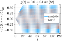
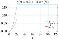
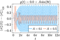
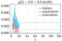
Figure S3: Crash test at $\mathbf{g=0}$. Top row: The periodic driving $\delta g(t)=A\sin(8t)$ at $g=0$ with amplitude $A=0.1$ for time $2\pi$ results in a large amplitude of transverse oscillations. The amplitude is lower than predicted by (28) due to the hard-core nature of bosons $b_{n}$ that is not quite negligible when their density $0.1$. Almost all quasiparticles/kinks are bound into pairs; densities of longer trains are at $10^{-4}$ or lower. Bottom row: Upon closer inspection, the oscillations for $A=0.1$, and even more $0.5$, have an admixture of frequency $4$ in addition to the main $\omega=8$. It is a manifestation of $4$-kink trains with density $0.00008$ and $0.001$ respectively.

Appendix F Crash test at $\mathbf{g=0}$

Here, we test the theory for strong periodic driving. It is the simplest at $g=0$ when a Bogoliubov quasiparticle is just a kink,

$$\gamma_{n}=k_{n},$$ (S52)

and the Hamiltonian simplifies to

$$H = -L+6\sum_{n}\gamma_{n}^{\dagger}\gamma_{n}-4\sum_{n}\gamma_{n}^{\dagger}\gamma_{n+1}^{\dagger}\gamma_{n+1}\gamma_{n}.$$ (S53)

The basic theory ignores that the pairs created by $b_{n}^{\dagger}=\gamma^{\dagger}_{n}\gamma^{\dagger}_{n+1}$ are not exactly bosons. It also ignores trains of kinks/quasiparticles longer than the pair. The trains also make bound states. Their energy at $g=0$ is $6n-4(n-1)=2n+4=6,8,10,12,...$ for $n=1,2,3,4,...$. At nonzero $g$ the terms (19) can transform a train of $n>2$ quasiparticles into one with $n-2$ — that has lower energy — making the longer trains unstable. This mechanism does not exist at $g=0$.

In Fig. S3, we drive $\delta g(t)=A\sin(8t)$ with $A=0.1,0.5$ for time $2\pi$. $A=0.1$ is enough to excite large transverse field oscillations that do not quite agree with (28). In addition to the lower amplitude of the main frequency $\omega=8$, there is an admixture of frequency $4$. Both effects become stronger for the stronger driving with $A=0.5$, which increases the density of excited kinks. The frequency $4$ originates from a superposition between a train of 4 kinks (energy $12$) and a pair of kinks (energy $8$), e.g.

$$\alpha\ket{...\uparrow\uparrow\downarrow\uparrow\uparrow\uparrow\uparrow...}e^{-8it}+\beta\ket{...\uparrow\uparrow\downarrow\uparrow\downarrow\uparrow\uparrow...}e^{-12it},$$ (S54)

where the corresponding $...$ are the same in both states. The states differ by one reversed spin; hence, $\sigma^{x}$ has a non-zero matrix element between them, and its expectation value oscillates with frequency $12-8=4$.

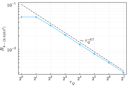
Figure S4: Amplitude of oscillations. The amplitude of oscillations after a smooth KZ ramp ending at $g=0.5$ with a protocol $g(t)=g_{c}[2-(1-0.5/(2g_{c}))(1+\sin(t/\tau_{Q}))]$, $t\in[-\tau_{Q}\times\pi/2,\tau_{Q}\times\pi/2]$).

Appendix G Amplitude of oscillations after KZ ramp

After a KZ ramp the number of kinks $\rho\propto\tau^{-1/2}$ as expected for this universality class  [1]. The frequency of the persistent oscillations is consistent with Fig. 3. Their amplitude depends on the ramp time with a power law $\tau^{-0.7}$, see Fig. S4.

A simple estimate for the exponent is as follows. After crossing the phase transition the density of excited $\gamma$-quasiparticles is $\rho\propto\tau^{-1/2}$. Near the crossover at $g_{0}$, when the bound pairs begin to have lower energy, the number of pairs can be roughly estimated as $\rho_{p}\propto\rho^{2}\propto\tau^{-1}$. The amplitude is proportional to the square root of $\rho_{p}$, compare the simple example in (23), and should scale as $\tau^{-0.5}$. The $0.5$ is close to the $0.7$ but appreciably different. Some more complex physics is missing in the simple argument.