Argon in $\beta$ Pictoris – entrapment and release of volatile in disks

Abstract

Chemical compositions of planets reveal much about their formation environments. Such information is well sought-after in studies of Solar System bodies and extra-solar ones. Here, we investigate the composition of planetesimals in the $\beta$ Pic debris disk, by way of its secondary gas disk. We are stimulated by the recent JWST detection of an Ar II emission line, and aim to reproduce extensive measurements from the past four decades. Our photo-ionization model reveals that the gas has to be heavily enriched in C, N, O, and Ar (but not S and P), by a uniform factor of about 100 relative to other metals. Such an abundance pattern is both reminiscent of, and different from, that of Jupiter’s atmosphere. The fact that Ar, the most volatile and therefore the hardest to capture into solids, is equally enriched as C/N/O suggests that the planetesimals were formed in a very cold region ($T\leq 35\,\rm K$) with abundant water ice. In the debris disk phase, these volatile are preferentially outgassed from the dust grains, likely via photo-desorption. The debris grains must be ’dirty’ aggregates of icy and refractory clusters. Lastly, the observed strength of the Ar II line can only be explained if the star $\beta$ Pic (a young A6V star) has sizable chromospheric and coronal emissions, on par with those from the modern Sun. In summary, observations of the $\beta$ Pic gas disk rewind the clock to reveal the formation environment of planetesimals.

1 The Motivations

The recent JWST detection of the Ar II 6.986 $\mu$m line (Worthen et al., 2024) reignited our interest in the gas disk around $\beta$ Pic. It comes as a surprise that Argon, a noble gas with a lower abundance than many other elements, should emit the brightest line in the mid-infrared (MIR). Our investigation into this surprise uncovers interesting information.

At a distance of $\sim 19$ pc, and spatially extended ($\sim 100$ au), the $\beta$ Pic debris disk is a favourite object for many studies. Both its gas and dust components have been extensively mapped (see, e.g., Chen et al., 2007, and references therein), to study the origin of debris disks. The gas component, likely sourced from the dust grains, yields kinematic information unavailable if only the dust component is visible.

The gas in $\beta$ Pic and other debris disks also opens a profitable window into another issue, chemical composition of the parent planetesimals. As such information is intimately related to the formation history, it has been actively sought after. For example, for Solar system bodies, the abundances of volatile gases and noble gases are often measured by expensive space missions (see reviews by Hersant et al., 2004; de Pater et al., 2023). In debris disks with gas components, these elements are in plain view and can be measured with the simple act of taking a spectrum.

atom/ion	measured	references	model
	[$\,\rm cm^{-2}$]		[$\,\rm cm^{-2}$]
H0	$<{\rm a\,few}\times 10^{19}$	[12]	$4.5\times 10^{17}$
H+			$6.5\times 10^{17}$
C0	$3\times 10^{16}$ †	[2]	$7.2\times 10^{16}$
C+	$2\times 10^{16}$ †	[5]	$2.3\times 10^{17}$
C++	$1.3\times 10^{13}$	[3]	$9.5\times 10^{12}$
N0	$8\times 10^{14}$ †	[4]	$4.2\times 10^{16}$
N0	$8\times 10^{16}$	[this work]	$4.2\times 10^{16}$
N+			$3.4\times 10^{16}$
O0	$5\times 10^{15}$ †	[5]	$2.9\times 10^{17}$
O+			$2.6\times 10^{17}$
Ar0			$1.3\times 10^{15}$
Ar+			$1.5\times 10^{15}$
Ne0			$9.5\times 10^{14}$
Ne+			$7.0\times 10^{12}$
Na0	$4.5\times 10^{10}$	[11]	$4\times 10^{10}$
Na+	$>3\times 10^{13}$	[5]	$2.0\times 10^{13}$
Mg0	$2.5\times 10^{11}$	[6]	$1.3\times 10^{12}$
Mg+	$>2\times 10^{13}$	[7]	$4.4\times 10^{14}$
Al0	$<4\times 10^{10}$	[7]	$6.5\times 10^{7}$
Al+	$4.5\times 10^{12}$	[7]	$3.2\times 10^{13}$
Si0	$<10^{13}$	[7]	$1.4\times 10^{12}$
Si+	$10^{14}$	[7]	$3.6\times 10^{14}$
P0	$<7\times 10^{11}$	[5]	$5.8\times 10^{10}$
P+	$<9.2\times 10^{13}$	[5]	$2.8\times 10^{12}$
S0	$5.4\times 10^{12}$	[7]	$2.1\times 10^{12}$
S+			$1.4\times 10^{14}$
S++	$<4\times 10^{11}$	[4]	$1.7\times 10^{10}$
Ca0	$3\times 10^{8}$	[8]	$4.7\times 10^{8}$
Ca+	$1.26\times 10^{13}$	[9]	$2.3\times 10^{13}$
Ca++			$1.9\times 10^{12}$
Cr0			$9.8\times 10^{9}$
Cr+	$3.5\times 10^{12}$	[7]	$4.6\times 10^{12}$
Mn0	$<3\times 10^{10}$	[7]	$5.4\times 10^{9}$
Mn+	$3\times 10^{12}$	[7]	$3.0\times 10^{12}$
Fe0	$10^{12}$	[7]	$4.0\times 10^{11}$
Fe+	$3.7\times 10^{14}$	[10]	$3.7\times 10^{14}$
Ni0	$<7.6\times 10^{10}$	[5]	$2.9\times 10^{10}$
Ni+	$1.5\times 10^{13}$	[7]	$1.8\times 10^{13}$
Zn0	$<7\times 10^{10}$	[7]	$3.7\times 10^{10}$
Zn+	$2\times 10^{11}$	[7]	$3.7\times 10^{11}$

Table 1: Column densities for various atoms and ions, both measured from absorption line studies (errorbars suppressed) and calculated in our model. † marks those obtained from unresolved UV absorption lines and may be plagued by saturation; these should be st considered as lower limits. References: [1] Wilson et al. (2017); [2] Roberge et al. (2000); [3] Bouret et al. (2002); [4] Wilson et al. (2019); [5] Roberge et al. (2006); [6] Vidal-Madjar et al. (1994); [7] Lagrange et al. (1998); [8] Kiefer et al. (2019); [9] Crawford et al. (1994); [10] J. Debbs; [11] Vidal-Madjar et al. (1986);[12] Freudling et al. (1995). We provide an updated N⁰ determination in Appendix B.

With the initial goal of explaining the Ar line, we carry out a study of the $\beta$ Pic gas disk. Our results serve to answer questions on two main directions: one, origin of gas in the $\beta$ Pic disk; and what do their abundance pattern reveal about the process of planet formation. We also provide some new JWST analysis of a few other emission lines (Appendix A).

1.1 Origin of gas in the $\beta$ Pic debris disk

Ever since its discovery four decades ago (Smith & Terrile, 1984), the debris disk around $\beta$ Pic has been under intense study. But it, especially its gas component, remains enigmatic to date. In the same way as the observed $\mu$m-sized dust must be recently generated, since their collisional lifetime is much less than the system age (Backman & Paresce, 1993), so must the gas be secondary in origin. Observed to be collocated with the dust (Brandeker et al., 2004; Nilsson et al., 2012), they are not remnant from the proto-planetary disk but are rather released from the orbiting debris (Wilson et al., 2017; Cataldi et al., 2018, 2023). Various hypothesis on how the gas is released have previously been presented: through dust sublimation, through collisional vaporization (Czechowski & Mann, 2007), through photo-desorption of icy particles (Artymowicz, 1997; Chen et al., 2007; Grigorieva et al., 2007), or through a combination of re-accretion and release (Cataldi et al., 2020).

Not only are we unsure how the gas is released, we are also uncertain about when. The spatial distribution of CO (Dent et al., 2014) and C⁰ (Cataldi et al., 2018) show a north-east/south-west disk asymmetry that implies a recent ($<5000$ yr) increase in CO gas production (Cataldi et al., 2018), as the C⁰ otherwise should have azimuthally sheared into a smooth ring and later diffused into an accretion disk (Kral et al., 2016). Recent observations by JWST/MIRI of dust emission shows a curved extension bending away from the disk and that seems connected to the CO asymmetry, implying a perhaps even more recent gas production event (100–200 yr) for the asymmetric component (Rebollido et al., 2024). Both these estimates are much shorter than the system lifetime of $\sim 20$ Myr (Mamajek & Bell, 2014). The origin of the above asymmetry is also unclear.

At least one puzzle on the gas disk is resolved. It has long been wondered why refractory elements such as Na, Ca and Fe, which experience strong radiation pressure (Beust et al., 1989), appear to orbit the star in nearly Keplerian orbits (Olofsson et al., 2001; Brandeker et al., 2004). Fernández et al. (2006) proposed that an excess of C, by a factor of $10$, is sufficient to brake the ions by Coulomb interactions. The C over-abundance in the gas disk was subsequently confirmed by Roberge et al. (2006); Cataldi et al. (2014) and naturally resolved the issue (also see Zagorovsky et al., 2010). In this work, we find that C/N/O are actually enriched by a factor of $100$, rendering radiation pressure completely unimportant. This also answers the question posed by (Xie et al., 2013): is the volatile enrichment caused by ‘preferrential production’ of volatiles, or ‘perferrential depletion’ of the refractories by radiation pressure? The answer is the former.

1.2 Observational constraints

The four decades of $\beta$ Pic observations have yielded a wealth of data, which we will compare our model against.

As the disk of $\beta$ Pic is seen edge on, its gas content was detected in absorption against the star (Slettebak, 1975) long before the discovery of the disk (Smith & Terrile, 1984). The initial assumption was that the gas is located within 1 au of the star (Lagrange et al., 1998), but later spatially resolved observations of Na I showed the emission to be co-located with the dust disk and the gas in orbits consistent with Keplerian velocities (Olofsson et al., 2001).

The edge-on geometry is a great advantage when constraining the column densities of various species, as using the star as a background light source enables very sensitive measurements of resonant transitions. In particular in the UV, many elements have strong transitions from the ground state. Table 1 shows column densities of some 30 atomic and ionic species, inferred from absorption line studies.

Column densities do not directly constrain where along the line of sight the absorbers are located. Complementary studies of spatially resolved scattered emission from resonance lines in atoms and ions (in particular from Na I, Fe I, and Ca II, see Olofsson et al., 2001; Brandeker et al., 2004; Nilsson et al., 2012) were therefore important to constrain the spatial extent of the disk.

Since the disk gas is expected to be relatively cold (Fig. 2), only low-energy fine-structure and molecular states are expected to be collisionally excited, with transitions in the infrared to sub-millimeter. See Table 2 for detected fine-structure emission lines from the disk gas. Among these, the C I 610$\mu$m line was spatially resolved (Cataldi et al., 2018). Table 2 also includes 3 new lines from JWST that are published here for the first time (Appendix A). We also present the spatial information we obtain from JWST on these lines in Table 3.

Here, we focus on atomic (and ionic) species. While some molecular lines are also observed, they are less informative and are unimportant for the overall thermal/chemical budget. We also only consider the so-called ‘stable’ gas of the main disk – gas at heliocentric velocities $\sim 20$ km s^-1 ($\beta$ Pic’s stellar velocity) – and not the temporally variable gas absorption features that have been interpreted as Falling Evaporating Bodies (FEBs, Beust et al., 1989).

Many resonant transitions in the UV in particular are so strong that they become strongly optically thick. In combination with unresolved complex line profiles, it becomes difficult to constrain the column densities with high accuracy, as the observed, unresolved line becomes a non-linear function of the actual line profile. An example is the determination of the O column density (Roberge et al., 2006) that was later found to likely have been underestimated (Brandeker et al., 2016). A similar instance concerns the column density of N I (Wilson et al., 2019, hereafter W19), where the 1200 Å triplet as observed with HST/COS was found to be strongly optically thick and best fit with multiple unresolved line components. Since their derived constraint implied a N⁰ column density that lies about two orders of magnitudes below our prediction (Fig. 6), we decided to have a closer look to better understand what an upper limit on the N column density would be that is still consistent with data. Our study is presented in Appendix B. We conclude that our predicted overabundance of N is indeed consistent with the HST/COS data, and maybe even preferred as the derived line profile better matches the observed absorption lines.

cooling line	observed flux	spectral res.	spatial res.	references	model flux
	[$\,\rm erg/\,\rm s/\,\rm cm^{2}$]	[km/s]			[$\,\rm erg/\,\rm s/\,\rm cm^{2}$]
C II 158 $\mu$m	$(2.4\pm 0.1)\times 10^{-14}$	$0.17$	no	Cataldi et al. (2014)	$2.2\times 10^{-14}$
C I 610 $\mu$m	$(1.6\pm 0.2)\times 10^{-16}$	$0.34$	yes	Cataldi et al. (2018)	$2.7\times 10^{-16}$
O I 63.2 $\mu$m	$(1.24\pm 0.25)\times 10^{-14}$	$86$	no	Brandeker et al. (2016)	$1.2\times 10^{-14}$
Ar II 6.99 $\mu$m	$2.4{\pm 0.1}\times 10^{-14}$	$88$	yes	Worthen et al. (2024)	$2.6\times 10^{-14}$
Ne II 12.81 $\mu$m	$<2\times 10^{-15}$	$88$	-	this work	$3.4\times 10^{-17}$
Fe II 17.93 $\mu$m	$4.3{\pm 0.5}\times 10^{-15}$	$88$	yes	this work	$1.6\times 10^{-15}$
Fe II 25.99 $\mu$m	$1.1{\pm 0.1}\times 10^{-14}$	$88$	yes	this work	$9.4\times 10^{-15}$

Table 2: Atomic cooling lines detected from the $\beta$ Pic gas disk. See Appendix A for some new measurements.

1.3 Volatiles and Planet Formation

Regardless of the gas production mechanism, the gas composition reflects the composition of their parent bodies, and places constraint on the formation of these bodies.

As will become clear below, gas around $\beta$ Pic is highly enriched in volatiles like C/N/O and Ar. These elements are also sometimes called super-volatiles, as their main carriers in the proto-planetary disks (CO, N₂ and Ar) are notoriously difficult to be captured into solid bodies. Their existence in planets and moons thus provides a natural thermometer for the formation environment. In the following, we briefly review the processes of volatile capture, before giving a short re-cap of Solar system measurements that are pertinent to our study.

There are 3 known ways to capture volatiles: direct condensation; entrapment by porous water ice (Bar-Nun et al., 1988); and clathrate hydrate formation in crystalline water ice (Lunine & Stevenson, 1985). Direct condensation of Ar, N₂ and CO require, for nebula pressure and solar abundances, extremely low temperatures, $T<25$ K (see, e.g., Iro et al., 2003; Hersant et al., 2004).

In comparison, entrapment by water ice (either by porosity or through clathration) enables volatile capture at higher temperatures, ranging from (Iro et al., 2003; Bar-Nun et al., 1988; Ninio Greenberg et al., 2017; Simon et al., 2023) 45 K for CO (the most stable volatile), to 40 K for N₂, and to 35 K for Ar (the hardest to trap). At temperatures below $35\,\rm K$, all hyper-volatiles can be indiscriminately trapped.

The entrapment processes depend on the abundance of water. As more stable volatiles (e.g., CO and N₂) take up available host sites first (Lunine & Stevenson, 1985; Iro et al., 2003), a shortage of water may lead to a strong depletion of the more volatile gases (e.g., Ar). We can estimate the amount of water required, in terms of the ratio $N_{\mathrm{O}}/N_{\mathrm{C}}$. As each CO or N₂ molecule requires $5-6$ H₂O molecules as hosts (Hersant et al., 2004), complete Ar capture suggests that $N_{\mathrm{O}}/N_{\mathrm{C}}\geq 4.4$ (for a solar ratio of $N_{\mathrm{C}}/N_{\mathrm{N}}=4$). This is larger than the solar vlaue of $(N_{\mathrm{O}}/N_{\mathrm{C}})_{\odot}\sim 1.8$.

A number of volatiles have been measured in Jupiter’s atmosphere, by ground-based observations and space missions like Voyager, Galileo and Juno (for a recent review, see de Pater et al., 2023). It appears that Jupiter is uniformly enriched in C, N, O, S, P, Ar, Kr, and Xe, by about a factor of 3 (Atreya et al., 1999; Li et al., 2020). This uniform enrichment, including even the most volatile Ar, suggests that the solids that are responsible for enriching Jupiter’s atmosphere are formed at a very cold locale in the solar system, where $T<35\,\rm K$ (Owen et al., 1999; Öberg & Wordsworth, 2019). This is much cooler than that expected for a passively irradiated disk at 5 au ($T\sim 75\,\rm K$, Chiang & Goldreich, 1997) and remains a puzzle (Owen et al., 1999; Öberg & Wordsworth, 2019). Moreover, if these volatiles are trapped by water ice (only), one requires a minimum oxygen over-abundance of

$${{(N_{\mathrm{O}}/N_{\mathrm{H}})}\over{(N_{\mathrm{O}}/N_{\mathrm{H}})_{\odot}}}={{(N_{\mathrm{O}}/N_{\mathrm{C}})(N_{\mathrm{C}}/N_{\mathrm{H}})}\over{(N_{\mathrm{O}}/N_{\mathrm{H}})_{\odot}}}$$

$$={{4.4\times 3\times(N_{\mathrm{C}}/N_{\mathrm{H}})_{\odot}}\over{(N_{\mathrm{O}}/N_{\mathrm{H}})_{\odot}}}={{4.4\times 3}\over{1.8}}\sim 7\,.$$ (1)

In this regard, it is interesting to note that Li et al. (2024) updates the Jupiter’s O over-abundance from $3$ to the preferred value 4.9 times solar, with a possible range 1.5–8.3.

Measurements on other Solar system bodies are more sparse. Existing measurements on Saturn, Uranus and Neptune suggest that they are also heavily enriched in the volatile elements (C, S, and P). Measuring their abundances in elements like Ne, Ar, Kr and Xe remains to be a key objective of future space missions (e.g., Atreya et al., 2018; Simon et al., 2018). Objects at larger distances, e.g., Titan (a moon of Saturn) and Oort cloud comets, are surprisingly very depleted in Ar and/or N (Niemann et al., 2005; Balsiger et al., 2015), in contrast to the cold condition inferred for Jupiter, making for a confusing interpretation.

Given this state, data from other systems are much welcomed. As we will show in this work, gas observations in the $\beta$ Pic debris disk open a new window towards understanding volatile reservoirs in outer planetary systems.

1.4 This Work

Our main tool here is the CLOUDY spectral synthesis code (Ferland et al., 2013). We will construct a model that contains two major ingredients: first, the gas disk (gas radial distribution, abundance pattern), and second, the star itself. Although $\beta$ Pic is a bright main-sequence A6V star, its radiation is far from being well understood. Unexpected high UV and X-ray emission of unclear origin has been observed from the star. These high-energy radiations dramatically affects the ionization balance in the gas disk, and hence its emission/absorption properties. We will introduce our model for the star and the gas disk in §2–3, respectively; in §3.2, we use CLOUDY to infer the elemental abundances that are consistent with observational constraints. We then discuss the implications of our results, both for the origin of gas in debris disks (§4), and for the elemental abundances of planetesimals (§5).

2 Model for the Stellar Emission

We adopt a photospheric model of $T_{\rm eff}=8052\,\rm K$ interpolated from the ATLAS model (Castelli & Kurucz, 2003), with a bolometric luminosity of $8.7\,L_{\odot}$ (Crifo et al., 1997). Since the metallicity of $\beta$ Pic is found to be insignificantly different from solar ([Fe/H] = 0.11 $\pm$ 0.1, Saffe et al., 2008), we assume it to be exactly Sun-like.

In addition to the photospheric radiation, we assume that the star contains two more components that are important for the gas disk: a hot, tenuous corona, and a denser, somewhat cooler chromosphere below the corona.

2.1 Chromosphere model

Argon has a first ionization potential of 15.7 eV, at which the photospheric flux is negligible. So a hot chromosphere is essential to explain the observed Ar II emission (and also the C II line). In addition, continuum UV photons from the chromosphere are important for heating the gas disk.

Empirically, gas hotter than the photosphere has also been known to exist on $\beta$ Pic, as evidenced by the strong emission lines in Ly $\alpha$ and O V (W19), and C III, C IV, and O VI (Bouret et al., 2002). These lines have equivalent widths of a few hundred  km s^-1. The luminosity in the Ly $\alpha$ line alone amounts to a few $\times 10^{-5}\,L_{\odot}$ (W19).

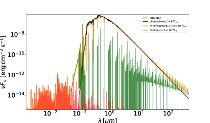
Figure 1: Our modelled emissions from the stellar photosphere, chromosphere and corona. The chromosphere mostly emits in FUV, though it also contributes in many line emissions. The corona is seen in X-rays.

These are all highly suggestive of a hot chromosphere. Bouret et al. (2002) constructed a simple model that is composed of a thin layer of gas ($N_{\mathrm{H}}$ $\sim 3\times 10^{20}$ cm^-2) with a temperature that ranges from $10^{4}$ to $10^{5}\,\rm K$. They obtained a cooling luminosity $2.5\times 10^{-5}\,L_{\odot}$ in these lines alone. We follow their lead but invoke an even simpler model, one where the column density is the same as theirs, but where the temperature is constant. We increase the temperature from the photospheric value upwards, until the observed fluxes in the C II and O VI lines can be reproduced. We find $T\sim 1.3\times 10^{4}\,\rm K$. For this simple model, the radiative cooling luminosity, emitted mostly in the UV continuum, is $\sim 3\times 10^{-3}\,L_{\odot}$, comparable to that of the Solar chromosphere. This energy is likely provided, as in the case of the Sun, from the mechanical heating of acoustic or Alfvén waves, excited below the photosphere.

2.2 Corona model

X-ray photons are also detected from $\beta$ Pic (Hempel et al., 2005; Günther et al., 2012). We again adopt a single one-zone model for the corona. The temperature is taken to be $1.1\times 10^{6}\,\rm K$, as determined by Günther et al. (2012). The total coronal luminosity is set to be $5\times 10^{-8}L_{\odot}$, to be compatible with the observed x-ray fluxes. This value is lower than the Solar coronal luminosity of $10^{-6}L_{\odot}$.

The coronal emission is too weak to affect the energy budget of the disk gas, but it does enhance the abundances of some highly ionized species (e.g., C⁺⁺, S⁺⁺).

The combined stellar emission spectrum is shown in Fig. 1. The chromosphere and corona dominate over the stellar photosphere in wavelengths shortwards of $0.1\,\mu$m.

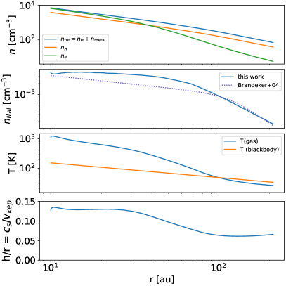
Figure 2: Radial structure of our model gas disk. The top panel shows the run of number densities with radius: total (metal+hydrogen), hydrogen and electron. Most of the electrons are contributed by C/O. The second panel compares the Na I mid-plane number density, as calculated in our model and as empirically determined by Brandeker et al. (2004, their eq. 1). The third panel displays the temperatures of gas (as determined by CLOUDY) and dust (black-body, zero albedo). The last panel is the vertical gas scale height for hydrostatic equilibrium.

2.3 Accretion onto $\beta$ Pic?

It is surprising that $\beta$ Pic, a A6V star (also a $\delta$-Scuti variable), should host a chromosphere and corona, structures that are usually associated with stars of later spectral types. Could the X-ray and UV emission be powered by gas accreting onto the star?

The line luminosities in the UV amount to a few $10^{-5}\,L_{\odot}$ (Bouret et al., 2002), and can be powered by an accretion at the rate of $\dot{M}\sim 6\times 10^{-13}\,M_{\odot}$ yr^-1. This is already higher than a crude estimate from King & Patten (see, e.g. 1992). But it gets worse. To produce these lines, the hot gas requires a sufficient column (see above section). It will then also emit in the continuum, and according to our model, at the much higher luminosity of $3\times 10^{-3}\,L_{\odot}$. If accretion is to supply this, an unrealistically high accretion rate of $10^{-10}\,M_{\odot}$ yr^-1 is required.

The total mass of the $\beta$ Pic gas disk is estimated to be $\sim 10^{25}\,\rm g$ (see below), so it could only supply the above high rate for $\sim 40$ yr, i.e., a couple of dynamical time scales at 10 au. Accreting disk gas can thus not be responsible for the UV emission.

3 Disk Model and Comparison with Observations

3.1 Disk Model

Here, we introduce a model for the gas disk that can reproduce the bulk of the observables. The model is deliberately kept as simple as possible, ignoring many complications (e.g., detailed radial profile, vertical distribution, azimuthal asymmetry, dust).

We assume the gas disk to extend from 10 to 200 au, with a (vertically constant) number density of H that goes as

$$n_{\mathrm{H}}=220{\,\rm cm^{-3}}\,\left[\left({r\over{100\,{\rm au}}}\right)^{2.5}+\left({r\over{100\,{\rm au}}}\right)^{4.6}\right]^{-1/2}\,.$$ (2)

This is similar in form but slightly different in parameters from that adopted by Zagorovsky et al. (2010). It ensures that our derived Na I profile closely emulates the observed one (Brandeker et al., 2004; Nilsson et al., 2012), as is shown in Fig. 2. The bulk of the gas lies at around 100 au, consistent with the C II study by Cataldi et al. (2014). While our chosen outer cutoff is motivated by the observed extents of the gas dust disks, and does not strongly impact the results, the inner cutoff requires some explanations. Our choice of inner cut-off is motivated by the study of Brandeker et al. (2004), where they observed Na I emission from 13 to 323 au. In agreement, the kinematically resolved profile of the C II 158 $\mu$m line shows flux from only outside 10 au (Cataldi et al., 2014). We also find best agreement with data when a limit is set at 10 au. Intriguingly, 10 au is also the semi-major axis of the giant planet $\beta$ Pic b.

Vertically, our model disk extends a height of $H/r=0.2$ from the midplane (or covering a solid angle $\Omega=4\pi\times 0.2$ sr). This is somewhat thicker than the self-consistently calculated gas scale height, $H/r=c_{s}(T)/v_{\rm kep}$, which ranges from $0.05$ to $0.13$ (Fig. 2).

The composition of the disk is unusual. We assume it to be depleted of primordial hydrogen and supplied by sublimation from icy grains. The $N_{\mathrm{H}}/N_{\mathrm{O}}$ number ratio is taken to be $2$, reflecting H₂O. We assume there is no He in the disk, since it is unlikely to be retained by condensation or calthration. We then assume C, N, and Ar are in solar proportion to O (solar composition from Asplund et al., 2009), while all other elements (see Fig. 6, called ‘refractory’ from now on) are reduced by a factor of $100$ from their solar values, again relative to O.

The total mass in this metal-rich disk amounts to $\sim 2\times 10^{25}\,\rm g$ ($\sim 0.3\,M_{\rm moon}$). Out of this mass, only a tiny fraction ($8\times 10^{22}\,\rm g$, or $0.3\%$) is contributed by the refractory elements. Moreover, the total mass of C is $\sim 6\times 10^{24}\,\rm g$ , consistent with that derived by Cataldi et al. (2018) using C I and C II lines.

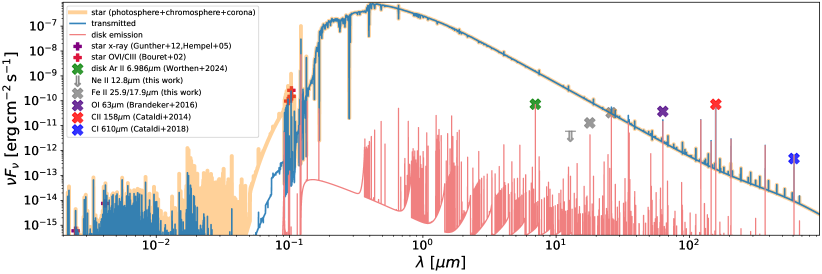
Figure 3: Spectral energy distributions in our model, including the stellar spectrum (original, including all three emission components; transmitted: after passing through the disk) and that of the disk emission. Spectral resolution for the lines is taken to be 100 km s^-1. The Ar II line is the dominant gas coolant in MIR, explaining its detection by JWST. Fluxes in various lines agree reasonably well with the observed values (colored symbols).

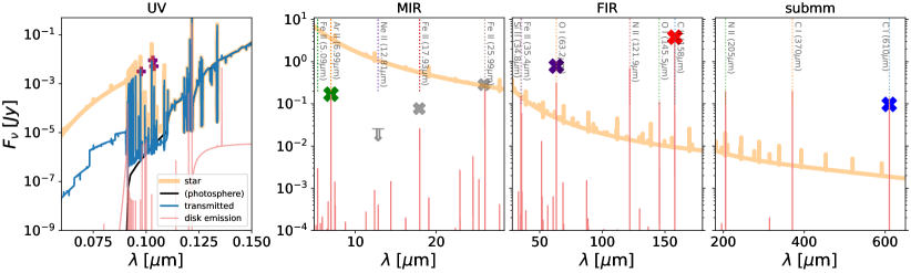
Figure 4: A close-up view of Fig. 3 in four wave-bands. Same notations except the vertical axis is now flux.

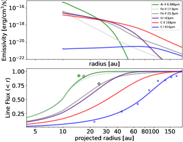
Figure 5: Comparing radial profiles for the few important cooling lines. The top panel shows line emissivity as a function of radius, while the lower one the integrated line fluxes out to a given projected radius, with the total flux normalized to unity. The three crosses indicate measurements from JWST (Appendix A), while the blue points are deduced from Cataldi et al. (2018). There are good overall agreements between model and data.

3.2 Comparisons

We use CLOUDY (Ferland et al., 2013) to compute the thermal and ionization balances in the gas disk, under the irradiation of our model star. The spectral resolution in the CLOUDY simulations is set to $100$ km s^-1. In Fig. 2, we show the resultant disk properties. Photo-ionization dominates disk heating and raises the disk temperature to over $1000\,\rm K$ near the inner boundary. This is dramatically hotter than those of previous models (Zagorovsky et al., 2010; Kral et al., 2016), and result from the high UV flux from our assumed chromosphere. The disk cools primarily through infrared and sub-mm metallic lines (including our main protagonist, the Ar II line), as well as the Ly$\alpha$ line.

CLOUDY also outputs the radiation signature of such a disk. Fig. 3 (and a zoomed-in version in Fig. 4) displays both the transmitted stellar spectrum (through an edge-on disk) and the emission spectrum from the disk itself. We compare these against observed values.

The transmitted stellar spectrum is consistent with the observed one. The edge-on disk absorbs most of the stellar UV, largely erasing the signature of the chromosphere except in some emission lines; the disk is transparent to the coronal X-ray.

The sub-mm/MIR disk lines have fluxes that agree within a factor of 2 or better with the observed values. These all arise from the volatile elements, C/O/Ar. It appears that, in combination, ALMA and JWST have captured most of the cooling luminosity from the disk.

For lines that are spatially resolved, we present a more fine-grained comparison in Fig. 5. As one moves outwards in disk, CLOUDY predicts that the gas cooling is sequentially dominated by the Ar II 6.986 $\mu$m line, the O I 63 $\mu$m line, and lastly, the C II 158 $\mu$m and C I 610 $\mu$m line. The Ar II line should be the most centrally concentrated because it requires a high UV flux, and we show in Appendix A that indeed the majority of its flux arises from inward of 20–30 au. A similar situation occurs for the two Fe II lines. In contrast, the C I line traces cold neutral gas and is the most spatially extended, with emissivity peaking near 100 au, again in good agreement with results from Cataldi et al. (2014). In fact, the apparent C I emission cavity (extending out to 50 au) as discussed by Cataldi et al. (2018) is not due to a genuine cavity but to the low emissivity of C I in the inner hot region.

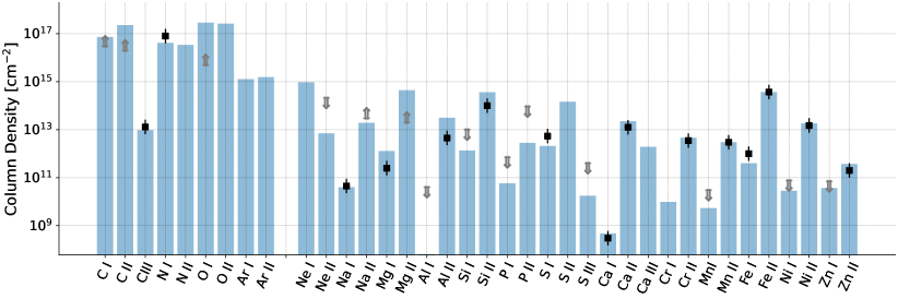
Figure 6: A comparison of the column densities of various elements and their ionized varieties, between those observed (black symbols, from Table 1, error bars indicate a factor of $2$ uncertainty, gray arrows indicate upper or lower limits) and calculated by CLOUDY (blue bars), where the left group (C, N, O, and Ar) are assumed to be enriched by $100\times$ over the other elements. There is an overall good agreement between the model and available constraints.

We now turn to a comparison with absorption line studies. Fig. 6 displays our predicted column densities for various atoms and ions, together with data from literature (Table 1). It is remarkable to observe that, while the data contain some 30 species and span some 8 orders of magnitude in values (including upper/lower limits), our simple model is able to hit the targets, mostly within a factor of two or better. In particular, while the original W19 determination of N⁰ would have indicated a depletion of N, which would be surprising astro-chemically, our new determination (Appendix B) brings N comfortably inline with other volatile species.

Lastly, we wish to emphasize the importance of the stellar chromosphere in these successes. If instead $\beta$ Pic does not possess a chromosphere, the resultant gas emission is shown in Fig. 7. The Ar II line is nearly absent, as there is not enough flux to ionize Ar (first ionization potential 15.6 eV). In general, photo-ionization heating is much reduced, leading to lower gas temperatures and much diminished cooling line fluxes. We also fail to reproduce the abundances of many ionized species.

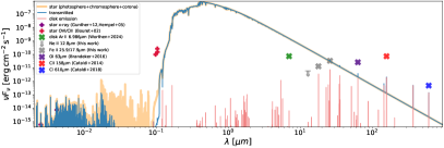
Figure 7: Same as Figs. 3 but for a model where the chromosphere is absent. The cooling line fluxes are all much reduced, most notably the Ar II line, as the gas is less photo-ionized and is cooler.

4 Gas production in Debris Disk

Our deduced abundances, a Solar-pattern except for a factor of 100 enhancement for C/N/O/Ar, place strong constraints on the capture process in the proto-planetary disk (next section), as well as on the release process in the debris disk (this section).

4.1 Preamble

Gas is most likely released from the dust grains. Here, we present grain properties pertinent to outgassing: temperature, dust mass and collision timescale. We assume that most of the dust surface area (for scattering and thermal emission) is provided by the smallest grains stable to radiation pressure, $s\sim 5\,\mu$m.

The blackbody temperature scales with radius as (with albedo $A_{b}$)

$$T_{\rm bb}=47\,\rm K\,(1-A_{b})^{-1/4}\,\left({r\over{100\,{\rm\,au}}}\right)^{-1/2}\,.$$ (3)

A 5 $\mu$m grain is slightly warmer than this, because it is inefficient in radiating at thermal wavelengths. We ignore this difference.

The dust mass can be estimated from the dust luminosity ($L_{\rm excess}/L_{*}\sim 2\times 10^{-3}$, e.g., Nilsson et al., 2009), which equals the fractional area covered by the grains, $N_{\rm grain}\pi s^{2}/(4\pi r^{2})$. Taking a grain bulk density of $\rho_{\rm grain}=1\,\rm g/\,\rm cm^{3}$ and placing all grains at $\sim 100$ au, we arrive at a small dust mass of $M_{\rm small-dust}=(4/3)\pi s^{3}\rho_{\rm grain}N_{\rm grain}\sim 2\times 10^{25}\,\rm g$, nearly the same as the total mass we have inferred above. This estimate does not include contribution from larger bodies.

To estimate the collision timescale, we assume that the debris disk is an annulus of radius $r\sim 100$ au, of width $\Delta r\sim r$, and a vertical scale height $H$. The radial optical depth of dust grains is $\tau_{r}\sim(L_{\rm excess}/L_{*})/(2H/r)$, and the vertical optical depth is,

$$\tau_{\perp}\sim\left({{2H}\over{r}}\right)\,\tau_{r}\sim\left({{L_{\rm excess}}\over{L_{*}}}\right)\sim 2\times 10^{-3}\,.$$ (4)

This is also the chance for grains to collide per half an orbit, yielding a mean collision time of

$$t_{\rm coll}\sim{1\over{2\tau_{\perp}}}\,P_{\rm orb}\sim\,2\times 10^{5}\,\rm yr\,\left({r\over{100\rm\,au}}\right)^{3/2}.$$ (5)

In comparison, the estimated stellar age is $\sim 20$ Myr.

4.2 Gas Release

To ensure a uniform enrichment of the volatiles in the gas, it is best if they are released from the grains via the same process. The hyper-volatiles (in the form of CO, N₂ and Ar) are efficiently thermally desorbed when temperature of the matrix (water ice) reaches $T\geq[35,40]\,\rm K$ (Simon et al., 2023). This is satisfied in most of the $\beta$ Pic disk (eq. 3, Fig. 2). In contrast, water ice cannot thermally desorb (sublimate) when $T\leq 100\,\rm K$, i.e., over much of the observed disk (also see Grigorieva et al., 2007).

In the high-UV environment of $\beta$ Pic, water can instead be released by photo-desorption (a.k.a. photo-sputtering), a non-thermal process of outgassing induced by UV photons. This was first proposed by Artymowicz (1997) and discussed in Chen et al. (2007); Grigorieva et al. (2007).

Theoretical calculations (Andersson & van Dishoeck, 2008) found that ice has a significant absorption cross section only in the 7.5 – 9.5 eV range (or 1300–1653 Å). Photons within this range are predicted and measured to have a desorption efficiency of $Y_{\mathrm{H_{2}O}}=$ 1 molecule/1000 UV photons. (Andersson & van Dishoeck, 2008; Westley et al., 1995; Öberg et al., 2009; Cruz-Diaz et al., 2018). Such a low value of $Y_{\mathrm{H_{2}O}}$ likely results from the layered structure – while UV photons can penetrate down to of order $\mu$m in depth, only those molecules liberated in the first handful of mono-layers can easily escape (Andersson & van Dishoeck, 2008; Öberg et al., 2009).

In $\beta$ Pic, such UV photons are mostly produced in the photosphere (and not in the chromosphere) and account for $\sim 10^{-3}$ of the total stellar flux. We find that a mono-layer of water ice (with an assumed molecular radius 3 Å) is lost after

$$t_{\rm photo,mono} \approx \left[{Y_{\mathrm{H_{2}O}}\times\left({L_{\rm UV}}\over{h\nu 4\pi r^{2}}\right)\times\pi(3\,\mathrm{\AA})^{2}}\right]^{-1}$$ (7)

$$\sim 0.1\,{\,\rm yr}\left({r\over{100\,{\rm au}}}\right)^{2}\,\,\left({{L_{\rm UV}}\over{10^{-3}L_{*}}}\right)^{-1}\,.$$

It takes a mere $(5\mu m/3\AA)\times t_{\rm photo,mono}\sim 1700\,\rm yr$ to evaporate a 5 $\mu$m grain, if it is made up of pure ice (also see Grigorieva et al., 2007). This is much faster than can be replenished by grain collisions (eq. 5). Moreover, given that $M_{\rm small-dust}\sim M_{\rm gas}$, evaporation at this high rate would build up the entire gas disk in a few thousand years. Both seem unreasonable. So the small grains observed in $\beta$ Pic cannot be predominately icy, a conclusion also reached by Grigorieva et al. (2007).

Realistic planetesimals are likely ’dirty’ – aggregates of ice (‘wet’) and refractory (‘dry’) clusters that result from condensation in the proto-planetary disk. The dry part, even at a few mono-layers thick, may stall volatile loss, for the same reason that $Y_{H_{2}O}$ is small (see above). Subsequent outgassing is possible after fresh icy surfaces are exposed by collision, or if the volatiles escape through narrow tunnels and surface cracks. Both may reduce the rate of water photo-desorption substantially.

Such a scenario of slow desorption may be tested by studying grain minerology. We expect the small grains in $\beta$ Pic to retain most of their refractories and some of their ices. The ices are buried below a thin layer of substrate but can resonantly scatter/emit photons with wavelengths longer than a few microns (for a thorough investigation, see Kim et al., 2019). As a result, the dust disk should appear bright in both the $10\,\mu$m silicate feature (as is indeed observed by Chen et al., 2007; Lu et al., 2022), and the $3\mu$m ice feature. So far, the ice signature has not been found in debris disks (Grigorieva et al., 2007; Rebollido et al., 2024), but we suggest that JWST should detect it.

Moreover, if the outgassing rate is determined by the local photon flux, as opposed to the local collision rate, this would explain why the gas distribution (eq. 2) roughly scales as the dust distribution (see, e.g. Fernández et al., 2006) multiplied by a factor $1/r^{2}$.

In summary, we suggest that water ice is photo-desorbed from small grains at a much reduced rate than theoretically possible, due to the ’dirty’ grain composition. The hypervolatiles are released concurrently with water, explaining the near-primordial C/N/O/Ar abundance pattern.

What about the refractory elements (including P/S)? Photo-desorption can directly release refractory elements. An early attempt by Chen et al. (2007) arrived at a Na desorption rate of $\sim 10^{18}\,\rm g\,\rm yr^{-1}$ in the $\beta$ Pic disk, based on limited lab experiments. But the desorption yield is poorly constrained, in particular, how the yield depends on photon energy and on atomic species is unknown. Given the near-solar abundance pattern, as well as a co-spatial distribution with the volatiles (see, e.g., Fig. 2), we instead suggest that they are more likely the by-product of volatile outgassing. But the actual process is unknown.

4.3 Alternative models and Caveats

Czechowski & Mann (2007) proposed to collisionally evaporate grains. They pointed out that collisions between bound grain (on largely circular orbits) and $\beta$ meteoroids (small grains radiatively accelerated to elliptical orbits) can reach speeds high enough for vaporization (e.g., $6.5\,\rm km/\,\rm s$ for ice and $\sim 19$ km s^-1 for silicates, Tielens et al., 1994). Based on a model of grain vaporization and fragmentation from Tielens et al. (1994), they calculated a gas production rate of $\sim 1.6\times 10^{19}\,\rm g\,\rm yr^{-1}$ for silicate, and about 40$\times$ higher than that for water. These appear competitive against photo-desorption. However, in such a theory (which contains inherent uncertainties, like the size distribution of $\beta$-meteoroids), one predicts that the volumetric outgassing rate should peak strongly where the dust lies ($\sim 100$au). In contrast, the observed gas density rises towards $10\,$au.

Czechowski & Mann (2007) also discussed sputtering by energetic particles in the stellar wind (Tielens et al., 1994). However, aside from the unknown strength of the stellar wind, the sputtering yield depends on the elements strongly (see Fig. 10 of Tielens et al., 1994). It is hard to forsee how this will generate anything close to the solar abundance pattern.

But similar to these alternative models, our favored scenario, photo-desorption, is also subject to uncertainties. In addition to those discussed in §4.2, the following caveats are present.

• There exists the possibility that the volatile gas can be re-absorbed onto grains, a process invoked to explain the HD 32297 disk (Cataldi et al., 2020). The timescale for gas-grain collision is competitive with photo-desorption and grain-grain collision timescales.

• The radial density profile, which we invoke to support photo-desorption, can be altered by magnetic stress, either via accretion (Kral et al., 2016) or via ejection by a magnetized wind. The absence of an inner accretion disk, as well as a strong azimuthal asymmetry in C I (Cataldi et al., 2018), both argue against a classical accretion disk.

• It remains an unexplained coincidence that the current gas disk is comparable in mass to that in the current generation of small grains. This is a surprise if the gas is accumulated over many collision times.

5 Elemental Abundances of Planet-forming Material

Our simple model have successfully reproduced a wide range of observables in the $\beta$ Pic disk. Here, we capitalize on this success to answer a second question: what could the abundance pattern in the $\beta$ Pic gas disk inform us about the planet formation process?

In this work, we find that Ar and N are just as enriched as C and O. Such a uniform enrichment, despite disparate physical/chemical properties, is best explained if almost all C, N, O, and Ar in the protoplanetary disk are retained, most probably by entrapment on (water)-ices. In fact, Ar/N place the strongest constraint as they are the hardest to trap. One requires a very cold environment, $T<35\,\rm K$. This is possible in the outer region of a passively irradiated proto-planetary disk, as the mid-plane temperature roughly goes as (Chiang & Goldreich, 1997)

$$T_{\mathrm{mid-plane}}\approx{35\,\rm K}\,\left(L_{*}\over{4\,\mathrm{L_{\odot}}}\right)^{1/4}\,\left({r\over{65\,{\rm au}}}\right)^{-3/7}\,,$$ (8)

where $L_{*}$ is the stellar luminosity during the disk phase.

Second, a complete trapping of C/N/Ar requires a large amount of O (see §1.3), about twice as much O as the solar value.

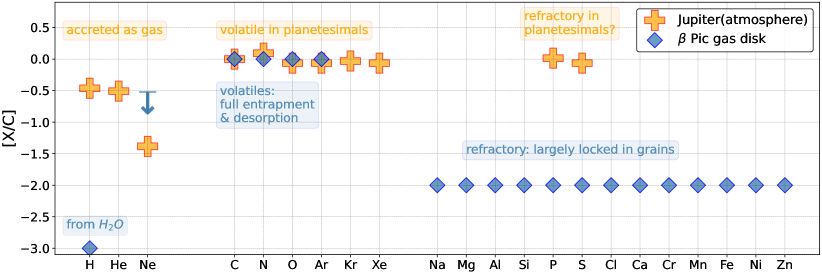
Figure 8: Comparison of abundance patterns in $\beta$ Pic gas disk (blue) and in Jupiter’s atmosphere (orange). All abundances are measured relative to C and normalized by the solar values. All error bars are suppressed for clarity. For $\beta$ Pic, Ne is marked by its upper limit, H/Ne is not yet confirmed. Text-boxes suggest possible pathways for these elements.

Fig. 8 compares the abundance pattern we infer for the $\beta$ Pic gas disk against the pattern in Jupiter’s atmosphere. For the latter, we adopt values compiled by Atreya et al. (1999) and updated in de Pater et al. (2023). There are clear agreements and disagreements, all deserving some thoughts. In the following, we discuss the comparison element by element:

• H and He: Current constraints on H and He in the $\beta$ Pic disk are weak. We assume that H is not primordial and is only derived from H₂O dissociation, and that He is not entrapped by planetesimals and is absent.

• Ne: similar to He, Ne has a small size and is difficult to entrap into solids (Lunine & Stevenson, 1985). So we do not expect to see Ne in the $\beta$ Pic disk, and that Ne is not enriched in Jupiter. Currently, a weak upper limit on Ne can be set using the Ne II $12.81\,\mu$m line (Table 2), corresponding to a column density of $N_{\mathrm{Ne\,II}}<10^{14}\,\rm cm^{-2}$ (Fig. 6), or that Ne can be at most a third as enriched as C/N/O/Ar.

  Any detectable amount of Ne would pose a strong challenge to the entrapment theory. The best way to hunt for Ne will likely be the Ne I absorption lines in the optical (e.g., 585, 640 nm), since Ne should mostly be in the form of Ne I due to the latter’s high ionization potential (21.56 eV). But these are transitions from excited states (not ground state) and may be challenging to detect.

• C and O: these are enhanced in both $\beta$ Pic and Jupiter. The actual value of $N_{O}/N_{C}$ is of major interest. Unfortunately, it is difficult to pin down in Jupiter due to surface meteorology. In $\beta$ Pic disk, however, a more careful model may be able to reach a higher accuracy than that that in our current model (a factor of two).

• N: the main carrier of $N$ in proto-planetary disks in $N_{2}$. Given its property, we expect N to be enhanced where-ever Ar is. Our new determination of $N^{0}$ supports this expectation. We advocate for further measurements. When released in the $\beta$ Pic disk, N₂ should be quickly broken down (photo-dissociation energy 9.76 eV) and show up as N⁰ or N⁺ at roughly the same proportion. They can be accessed by absorption line studies. CLOUDY also predicts strong N I 121.9 $\mu$m and N I 205 $\mu$m lines (Fig. 4).

• Ar, Kr, and Xe: known to be enriched uniformly (by $\sim 3\times$) in Jupiter’s atmosphere, we expect Kr and Xe to be as enriched as Ar in the $\beta$ Pic disk.

• S and P: these are two interesting species. We do not find them to be enriched like the volatiles (though the constraint on P is weaker), suggesting that they are incorporated into planetesimals in their refractory forms (e.g., FeS), not volatile forms (e.g., H₂S). This is consistent with the fact that S and P are heavily depleted in the ISM and in cold disks (Kama et al., 2019).

  This then begs the question of why Jupiter’s envelope is enriched in S and P. It is possible that these are released by bombarding planetesimals as they sublimate in Jupiter’s atmosphere. If so, all heavy elements (other than C/N/O/Ar/S/P) should be similarly enriched in Jupiter’s atmosphere.

These discussions make clear that, despite the different enrichment abundances, the planetesimals that outgas in the $\beta$ Pic disk are of similar composition to those that pollute the atmosphere of Jupiter.

6 Conclusion

We construct a radiative transfer model that successfully explains an array of observables in the $\beta$ Pic gas disk. There are two key elements in this model. First, the host star needs to harbour a hot chromosphere, allowing it to ionize Ar and other elements to their observed states. This may be surprising for an A-type star, but is supported by many other lines of evidence. Second, all elements follow roughly the solar pattern, except for an under-abundance of H (and possibly He), and an over-abundance of a uniform factor of $100$ for the volatile elements (C, N, O, and Ar). We argue that the planetesimals that produce the dusty debris have to be formed in regions where $T\leq 35\,\rm K$ and where water is abundant. This is similar to what has been suggested based on Jupiter’s atmospheric enrichment.

Stronger constraints on all of these elements will prove useful. Among these, we identify a few most interesting aspects: the C/O ratio, the noble gases, the N/S/P abundances.

The current gas mass in the $\beta$ Pic disk is $\sim 2\times 10^{25}\,\rm g$ (or $\sim 1/3$ lunar mass), similar to that in the current generation of small grains ($\sim 5\,\mu$m). We argue that water ices are likely desorbed off grains by the stellar UV fluxes, which then release the hyper-volatiles (C/N/Ar) they entrap. The refractories, we spectulate, may also be released in the same process, albeit at a rate reduced by a factor of $100$.

The photo-desorption rate, constrained by multiple lines of evidences, has to be much slower than that for pure-ice. So the grains are likely ‘dirty’ aggregates, made up of icy and silicate clusters and where desorption is slowed down by the silicate (or graphite) surfaces. This could be tested by grain minerology studies, by targeting the water-ice features. Understanding the microscopic structure of planetesimals can illuminate their formation process.

The trace amount of gas mass in $\beta$ Pic would have remained quite invisible, if not for the UV photons from the star: UV photons from the stellar photosphere desorb volatiles off the dust grains; then UV photons from the stellar chromosphere photo-ionize and heat the released atoms, making them visible to us in a multitude of emission and absorption lines. And by observing these signatures, we can unwind the clock to study an earlier phase, when the planetesimals form out of proto-planetary disks.

We thank the organizers of the Dust Devils workshop where this project was initiated. YW acknowledges support for research from NSERC, and helpful conversation with Peter Martin. KW and CC’s work are supported by the National Aeronautics and Space Administration under grant No. 80NSSC22K1752 issued through the Mission Directorate. AB acknowledges support from the Swedish National Space Agency.

Appendix A New measurements using JWST/MIRI MRS data

Line	Distance (au)	Flux (erg s-1cm-2)	Resolved Flux/Total Line Flux
Ar II	15–20	2.0$\pm$0.4$\times 10^{-15}$	0.08$\pm$0.02
Fe II 17.94 $\mu$m	17–22	4.1$\pm$0.8$\times 10^{-16}$	0.10$\pm$0.02
Fe II 25.99 $\mu$m	25–35	3.1$\pm$0.6$\times 10^{-15}$	0.22$\pm$0.05

Table 3: Spatially resolved line fluxes from the MIRI MRS data. The distance column shows the projected distance from the star covered by the extraction aperture. This distance corresponds to the 3$\sigma$ contours shown in Figure 10. The right most column shows the ratio of the resolved line flux to the total line flux.

We re-reduced the JWST MIRI MRS data of $\beta$ Pictoris that was presented in Worthen et al. (2024) with a newer version of the JWST pipeline (version 1.14.0, Calibrated Reference Data System context “jwst$\_$1223.pmap”) and detect two new Fe II lines. For a description of the observational parameters and setup, see Worthen et al. (2024). We processed the data using the exact same pipeline steps as Worthen et al. (2024), but then used the pipeline to extract the spectrum of the unresolved point source of $\beta$ Pic with an extraction aperture of 1.5$\times$ the PSF FWHM at each wavelength. Because we are only interested in the emission lines, we removed the continuum from the spectrum by subtracting a B-spline fitted to the spectral points outside of each of the emission lines. From this newly reduced spectrum, we detect Fe II emission lines at 17.936 and 25.988 $\mu$m and we also place an upper limit on Ne II at 12.838 $\mu$m. The two Fe II lines and the region of the spectrum containing the wavelength of the Ne II line are shown in Fig. 3.

We fitted the two Fe II lines with Gaussian profiles and then integrated the best-fit Gaussians to calculate the line flux of the spatially unresolved component of the line flux. The line fluxes are listed in Table 2. We calculated a 3$\sigma$ Ne II line flux upper limit by computing the standard deviation (1$\sigma$) of the 10 data points (5 on each side of the line) centered on the Ne II expected line location and used this as the peak line flux upper limit. We then used the average of the Ne II line widths in the upper limit calculation for Ne II. The upper limit of the Ne II line flux is shown in Table 2.

We also checked to see if the Fe II lines are spatially resolved like the Ar II line from Worthen et al. (2024). We did this by subtracting out a slice from the MRS data cube outside of the line from the slice at the peak of the line flux. This removes the resolved and unresolved emission from the dust and the central star, leaving only the emission from the Fe II lines. The spatially resolved components of the Fe II lines are shown in Fig. 10. We computed the spatially resolved line fluxes by extracting the spectra within the 3$\sigma$ red contours and outside of the JWST PSF FWHM shown in Fig. 10. We then fitted a Gaussian profile to the extracted line profile and integrated to get a resolved line flux. This was done on both sides of the disk and then summed together for each of the Fe II lines. The spatially resolved line fluxes of the lines from the MRS data are shown in Table 3.

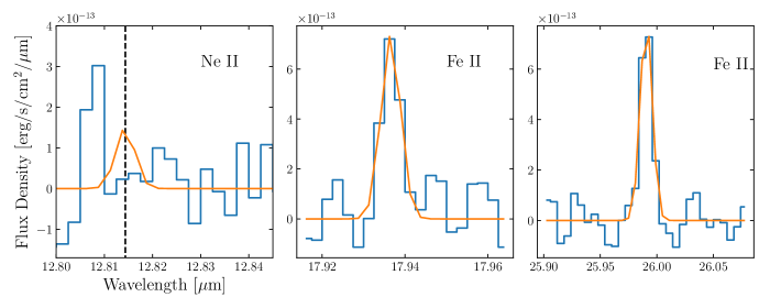
Figure 9: Left: MIRI MRS spectrum of the unresolved point source $\beta$ Pic over a wavelength range that contains the Ne II line at 12.81 $\mu$m. The black dashed line shows the expected location of the line at the radial velocity of $\beta$ Pic. The orange Gaussian is the corresponding line profile for the line flux upper limit we measure. Middle: Fe II line at 17.94 $\mu$m with best-fit Gaussian profile overlaid. Right: Fe II line at 25.99 $\mu$m with best-fit Gaussian profile overlaid.

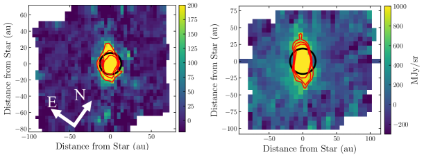
Figure 10: Left: PSF and continuum-subtracted MRS data cube slice at 17.94 $\mu$m showing the spatially resolved structure of the Fe II emission. The black circle shows the JWST PSF FWHM in the across slice direction at this wavelength and the red contours show 3, 5, and 10$\sigma$. Right: same as left but for the Fe II line at 25.99 $\mu$m. Note that the MRS Channel 4C PSF has a different FWHM in the across-slice and along-slice directions (see Law et al., 2023).

Appendix B Nitrogen from HST/COS data

Since constraining column densities from optically thick lines with complex profiles is challenging and often dependent on assumptions on the individual line components, we decided to have a closer look at the W19 constraints to see how high column density of N⁰ could reasonably be compatible with the data. We were kindly provided with the reduced and co-added HST/COS data used in W19 from the P. A. Strøm (né Wilson, priv. comm.). When attempting to reproduce their results we discovered that their model spectrum (their Fig. 1) used an approximately 0.5$\times$ too narrow line-spread function (LSF). This can be seen in the convolved N I lines of their Fig. 1, where their FWHM are closer to 10 km s^-1 rather than the expected 23 km s^-1 for the used instrument setting of COS. The consequence is that the column density of circumstellar N I becomes underestimated. Using the G130M/1222 LSF from LP3 downloaded from the STScI website (with FWHM $\approx$ 23 km s^-1), we find that many of the parameters used in W19 become more strongly correlated, e.g. the broadening parameter $b$ and column densities $N$ for the various absorption components. Using the broad LSF with the parameters found in W19 no longer produces a good fit (see Fig. 11). Adjusting the “stable circumstellar gas component” CS₀ of N I column density to a factor of 100$\times$ higher column density (i.e. $N_{\mathrm{N\,I}}=10^{16.9}$ cm${}^{-2}=7.9\times 10^{16}$ cm^-2) and fitting $b=1.4$ km s^-1 (from previous $b=1.0$ km s^-1), we get a much better match to the data (Fig. 11). Our conclusion is that a N overabundance of 100$\times$ compared to refractory elements is indeed consistent with the data.

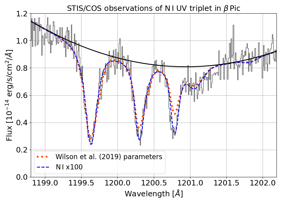
Figure 11: STIS/COS observations of the N I triplet of UV resonance lines (W19). The data are consistent with the ‘stable’ circumstellar N having a 100$\times$ overabundance relative to the refractory elements.

References

- Andersson & van Dishoeck (2008) Andersson, S., & van Dishoeck, E. F. 2008, A&A, 491, 907, doi: 10.1051/0004-6361:200810374
- Artymowicz (1997) Artymowicz, P. 1997, Annual Review of Earth and Planetary Sciences, 25, 175, doi: 10.1146/annurev.earth.25.1.175
- Asplund et al. (2009) Asplund, M., Grevesse, N., Sauval, A. J., & Scott, P. 2009, ARA&A, 47, 481, doi: 10.1146/annurev.astro.46.060407.145222
- Atreya et al. (2018) Atreya, S. K., In, J. H., & Hofstadter, M. D. 2018, in EGU General Assembly Conference Abstracts, EGU General Assembly Conference Abstracts, 9461
- Atreya et al. (1999) Atreya, S. K., Wong, M. H., Owen, T. C., et al. 1999, Planet. Space Sci., 47, 1243, doi: 10.1016/S0032-0633(99)00047-1
- Backman & Paresce (1993) Backman, D. E., & Paresce, F. 1993, in Protostars and Planets III, ed. E. H. Levy & J. I. Lunine, 1253
- Balsiger et al. (2015) Balsiger, H., Altwegg, K., Bar-Nun, A., et al. 2015, Science Advances, 1, e1500377, doi: 10.1126/sciadv.1500377
- Bar-Nun et al. (1988) Bar-Nun, A., Kleinfeld, I., & Kochavi, E. 1988, Phys. Rev. B, 38, 7749, doi: 10.1103/PhysRevB.38.7749
- Beust et al. (1989) Beust, H., Lagrange-Henri, A. M., Vidal-Madjar, A., & Ferlet, R. 1989, A&A, 223, 304
- Bouret et al. (2002) Bouret, J. C., Deleuil, M., Lanz, T., et al. 2002, A&A, 390, 1049, doi: 10.1051/0004-6361:20020741
- Brandeker et al. (2004) Brandeker, A., Liseau, R., Olofsson, G., & Fridlund, M. 2004, A&A, 413, 681, doi: 10.1051/0004-6361:20034326
- Brandeker et al. (2016) Brandeker, A., Cataldi, G., Olofsson, G., et al. 2016, A&A, 591, A27, doi: 10.1051/0004-6361/201628395
- Castelli & Kurucz (2003) Castelli, F., & Kurucz, R. L. 2003, in Modelling of Stellar Atmospheres, ed. N. Piskunov, W. W. Weiss, & D. F. Gray, Vol. 210, A20, doi: 10.48550/arXiv.astro-ph/0405087
- Cataldi et al. (2014) Cataldi, G., Brandeker, A., Olofsson, G., et al. 2014, A&A, 563, A66, doi: 10.1051/0004-6361/201323126
- Cataldi et al. (2018) Cataldi, G., Brandeker, A., Wu, Y., et al. 2018, ApJ, 861, 72, doi: 10.3847/1538-4357/aac5f3
- Cataldi et al. (2020) Cataldi, G., Wu, Y., Brandeker, A., et al. 2020, ApJ, 892, 99, doi: 10.3847/1538-4357/ab7cc7
- Cataldi et al. (2023) Cataldi, G., Aikawa, Y., Iwasaki, K., et al. 2023, ApJ, 951, 111, doi: 10.3847/1538-4357/acd6f3
- Cavallius et al. (2019) Cavallius, M., Cataldi, G., Brandeker, A., et al. 2019, A&A, 628, A127, doi: 10.1051/0004-6361/201935655
- Chen et al. (2007) Chen, C. H., Li, A., Bohac, C., et al. 2007, ApJ, 666, 466, doi: 10.1086/519989
- Chiang & Goldreich (1997) Chiang, E. I., & Goldreich, P. 1997, ApJ, 490, 368, doi: 10.1086/304869
- Crawford et al. (1994) Crawford, I. A., Spyromilio, J., Barlow, M. J., Diego, F., & Lagrange, A. M. 1994, MNRAS, 266, L65, doi: 10.1093/mnras/266.1.L65
- Crifo et al. (1997) Crifo, F., Vidal-Madjar, A., Lallement, R., Ferlet, R., & Gerbaldi, M. 1997, A&A, 320, L29
- Cruz-Diaz et al. (2018) Cruz-Diaz, G. A., Martín-Doménech, R., Moreno, E., Muñoz Caro, G. M., & Chen, Y.-J. 2018, MNRAS, 474, 3080, doi: 10.1093/mnras/stx2966
- Czechowski & Mann (2007) Czechowski, A., & Mann, I. 2007, ApJ, 660, 1541, doi: 10.1086/512965
- de Pater et al. (2023) de Pater, I., Molter, E. M., & Moeckel, C. M. 2023, Remote Sensing, 15, doi: 10.3390/rs15051313
- Dent et al. (2014) Dent, W. R. F., Wyatt, M. C., Roberge, A., et al. 2014, Science, 343, 1490, doi: 10.1126/science.1248726
- Ferland et al. (2013) Ferland, G. J., Porter, R. L., van Hoof, P. A. M., et al. 2013, Rev. Mexicana Astron. Astrofis., 49, 137, doi: 10.48550/arXiv.1302.4485
- Fernández et al. (2006) Fernández, R., Brandeker, A., & Wu, Y. 2006, ApJ, 643, 509, doi: 10.1086/500788
- Fraser et al. (2001) Fraser, H. J., Collings, M. P., McCoustra, M. R. S., & Williams, D. A. 2001, MNRAS, 327, 1165, doi: 10.1046/j.1365-8711.2001.04835.x
- Freudling et al. (1995) Freudling, W., Lagrange, A. M., Vidal-Madjar, A., Ferlet, R., & Forveille, T. 1995, A&A, 301, 231
- Grigorieva et al. (2007) Grigorieva, A., Thébault, P., Artymowicz, P., & Brandeker, A. 2007, A&A, 475, 755, doi: 10.1051/0004-6361:20077686
- Günther et al. (2012) Günther, H. M., Wolk, S. J., Drake, J. J., et al. 2012, ApJ, 750, 78, doi: 10.1088/0004-637X/750/1/78
- Hempel et al. (2005) Hempel, M., Robrade, J., Ness, J. U., & Schmitt, J. H. M. M. 2005, A&A, 440, 727, doi: 10.1051/0004-6361:20042596
- Hersant et al. (2004) Hersant, F., Gautier, D., & Lunine, J. I. 2004, Planet. Space Sci., 52, 623, doi: 10.1016/j.pss.2003.12.011
- Iro et al. (2003) Iro, N., Gautier, D., Hersant, F., Bockelée-Morvan, D., & Lunine, J. I. 2003, Icarus, 161, 511, doi: 10.1016/S0019-1035(02)00038-6
- Kama et al. (2019) Kama, M., Shorttle, O., Jermyn, A. S., et al. 2019, ApJ, 885, 114, doi: 10.3847/1538-4357/ab45f8
- Kiefer et al. (2019) Kiefer, F., Vidal-Madjar, A., Lecavelier des Etangs, A., et al. 2019, A&A, 621, A58, doi: 10.1051/0004-6361/201834274
- Kim et al. (2019) Kim, M., Wolf, S., Potapov, A., Mutschke, H., & Jäger, C. 2019, A&A, 629, A141, doi: 10.1051/0004-6361/201936014
- King & Patten (1992) King, J. R., & Patten, B. M. 1992, MNRAS, 256, 571, doi: 10.1093/mnras/256.3.571
- Kral et al. (2016) Kral, Q., Wyatt, M., Carswell, R. F., et al. 2016, MNRAS, 461, 845, doi: 10.1093/mnras/stw1361
- Lagrange et al. (1998) Lagrange, A. M., Beust, H., Mouillet, D., et al. 1998, A&A, 330, 1091
- Law et al. (2023) Law, D. R., E. Morrison, J., Argyriou, I., et al. 2023, AJ, 166, 45, doi: 10.3847/1538-3881/acdddc
- Li et al. (2020) Li, C., Ingersoll, A., Bolton, S., et al. 2020, Nat. Astron., 4, 609
- Li et al. (2024) Li, C., Allison, M., Atreya, S., et al. 2024, Icarus, 414, 116028, doi: 10.1016/j.icarus.2024.116028
- Lu et al. (2022) Lu, C. X., Chen, C. H., Sargent, B. A., et al. 2022, ApJ, 933, 54, doi: 10.3847/1538-4357/ac70d1
- Lunine & Stevenson (1985) Lunine, J. I., & Stevenson, D. J. 1985, ApJS, 58, 493, doi: 10.1086/191050
- Mamajek & Bell (2014) Mamajek, E. E., & Bell, C. P. M. 2014, MNRAS, 445, 2169, doi: 10.1093/mnras/stu1894
- Niemann et al. (2005) Niemann, H. B., Atreya, S. K., Bauer, S. J., et al. 2005, Nature, 438, 779, doi: 10.1038/nature04122
- Nilsson et al. (2012) Nilsson, R., Brandeker, A., Olofsson, G., et al. 2012, A&A, 544, A134, doi: 10.1051/0004-6361/201219288
- Nilsson et al. (2009) Nilsson, R., Liseau, R., Brandeker, A., et al. 2009, A&A, 508, 1057, doi: 10.1051/0004-6361/200912010
- Ninio Greenberg et al. (2017) Ninio Greenberg, A., Laufer, D., & Bar-Nun, A. 2017, MNRAS, 469, S517, doi: 10.1093/mnras/stx2017
- Öberg et al. (2009) Öberg, K. I., Linnartz, H., Visser, R., & van Dishoeck, E. F. 2009, ApJ, 693, 1209, doi: 10.1088/0004-637X/693/2/1209
- Öberg & Wordsworth (2019) Öberg, K. I., & Wordsworth, R. 2019, AJ, 158, 194, doi: 10.3847/1538-3881/ab46a8
- Olofsson et al. (2001) Olofsson, G., Liseau, R., & Brandeker, A. 2001, ApJ, 563, L77, doi: 10.1086/338354
- Owen et al. (1999) Owen, T., Mahaffy, P., Niemann, H. B., et al. 1999, Nature, 402, 269, doi: 10.1038/46232
- Rebollido et al. (2024) Rebollido, I., Stark, C. C., Kammerer, J., et al. 2024, AJ, 167, 69, doi: 10.3847/1538-3881/ad1759
- Roberge et al. (2000) Roberge, A., Feldman, P. D., Lagrange, A. M., et al. 2000, ApJ, 538, 904, doi: 10.1086/309157
- Roberge et al. (2006) Roberge, A., Feldman, P. D., Weinberger, A. J., Deleuil, M., & Bouret, J.-C. 2006, Nature, 441, 724, doi: 10.1038/nature04832
- Saffe et al. (2008) Saffe, C., Gómez, M., Pintado, O., & González, E. 2008, A&A, 490, 297, doi: 10.1051/0004-6361:200810260
- Simon et al. (2018) Simon, A., Banfield, D., Atkinson, D., & SPRITE Science Team. 2018, in American Astronomical Society Meeting Abstracts, Vol. 231, American Astronomical Society Meeting Abstracts #231, 144.01
- Simon et al. (2023) Simon, A., Rajappan, M., & Öberg, K. I. 2023, ApJ, 955, 5, doi: 10.3847/1538-4357/aceaf8
- Slettebak (1975) Slettebak, A. 1975, ApJ, 197, 137, doi: 10.1086/153493
- Smith & Terrile (1984) Smith, B. A., & Terrile, R. J. 1984, Science, 226, 1421, doi: 10.1126/science.226.4681.1421
- Tielens et al. (1994) Tielens, A. G. G. M., McKee, C. F., Seab, C. G., & Hollenbach, D. J. 1994, ApJ, 431, 321, doi: 10.1086/174488
- Vidal-Madjar et al. (1986) Vidal-Madjar, A., Hobbs, L. M., Ferlet, R., Gry, C., & Albert, C. E. 1986, A&A, 167, 325
- Vidal-Madjar et al. (1994) Vidal-Madjar, A., Lagrange-Henri, A. M., Feldman, P. D., et al. 1994, A&A, 290, 245
- Westley et al. (1995) Westley, M. S., Baragiola, R. A., Johnson, R. E., & Baratta, G. A. 1995, Nature, 373, 405, doi: 10.1038/373405a0
- Wilson et al. (2019) Wilson, P. A., Kerr, R., Lecavelier des Etangs, A., et al. 2019, A&A, 621, A121, doi: 10.1051/0004-6361/201834346
- Wilson et al. (2017) Wilson, P. A., Lecavelier des Etangs, A., Vidal-Madjar, A., et al. 2017, A&A, 599, A75, doi: 10.1051/0004-6361/201629293
- Worthen et al. (2024) Worthen, K., Chen, C. H., Law, D. R., et al. 2024, ApJ, 964, 168, doi: 10.3847/1538-4357/ad2354
- Xie et al. (2013) Xie, J.-W., Brandeker, A., & Wu, Y. 2013, ApJ, 762, 114, doi: 10.1088/0004-637X/762/2/114
- Zagorovsky et al. (2010) Zagorovsky, K., Brandeker, A., & Wu, Y. 2010, ApJ, 720, 923, doi: 10.1088/0004-637X/720/1/923