Pattern dynamics of the non-reciprocal Swift-Hohenberg model

Abstract

We investigate the pattern dynamics of the one-dimensional non-reciprocal Swift-Hohenberg model. Characteristic spatiotemporal patterns, such as disordered, aligned, swap, chiral-swap, and chiral phases, emerge depending on the parameters. We classify the characteristic spatiotemporal patterns obtained in the numerical simulations by focusing on the spatiotemporal Fourier spectrum of the order parameters. We derive a reduced dynamical system by using the spatial Fourier series expansion. We analyze the bifurcation structure around the fixed points corresponding to the aligned and chiral phases and explain the transitions between them. The disordered phase is destabilized either to the aligned phase or to the chiral phase by the Turing bifurcation or the wave bifurcation, and the aligned phase and the chiral phase are connected by the pitchfork bifurcation.

I Introduction

In recent years, the concept of non-reciprocity has attracted attention in the field of non-equilibrium physics, including pattern formation and active matter since non-reciprocity leads to novel non-equilibrium phenomena [1]. Non-reciprocity is often characterized by the violation of Newton’s third law by effective interactions [2, 3]. For example, microorganisms interact non-reciprocally through complex signal transduction mechanisms, which is known as quorum sensing and chemotaxis [4]. Moreover, non-reciprocity can induce new types of active phase separation phenomena [5, 6, 7, 8].

Recently, phase separation dynamics with non-reciprocity due to non-equilibrium chemical potentials have been studied by extending the gradient dynamics model with a free energy functional [8, 9, 10, 11]. Well-known continuum models describing phase separation are, for example, a non-conserved model represented by the Allen-Cahn equation [12] and a conserved model represented by the Cahn-Hilliard equation [13]. These equations can be derived by considering gradient dynamics with proper free energy functionals [14]. Some of the authors have examined the non-reciprocal Allen-Cahn (NRAC) model, which extends the Allen-Cahn equation to a non-reciprocal system, focusing on topological defects in two-dimensional (2D) systems [15]. There have been several studies on the non-reciprocal Cahn-Hilliard (NRCH) model [9, 16, 10, 11, 17, 18, 19, 20, 21, 22, 23, 24, 25, 8]. In the 2D NRCH model, for instance, non-reciprocity can lead to the emergence of characteristic patterns, such as targets and spirals, in which parity and time-reversal symmetry can be broken [17]. Generally, the introduction of non-reciprocity into gradient dynamics can lead to characteristic spatiotemporal dynamics, such as sustained oscillation and wave propagation.

The Swift-Hohenberg (SH) equation was originally introduced as a phenomenological model to describe the formation of roll patterns in thermal convection [26]. It can be derived from a non-conserved gradient dynamics model with a free energy functional. The SH equation has parameters associated with a convective instability and a characteristic wavenumber of emerging spatial patterns [27]. Several studies have been reported on the 1D coupled SH equations. Schuler et al. studied the coupled SH equations, in which two equations with different characteristic wavenumbers are coupled with non-reciprocal interaction [28]. Becker et al. re-examined the coupled SH equations with non-reciprocal interaction from the viewpoint of Turing and wave bifurcations [29]. Later, Fruchart et al. reported the qualitative pattern dynamics of the coupled SH equations with both reciprocal and non-reciprocal linear interaction terms [1]. Although they reported on characteristic spatiotemporal patterns, the detailed bifurcation structure remains unexplored.

In this study, we focus on the bifurcation structure of the non-reciprocal Swift-Hohenberg (NRSH) model. We classify characteristic spatiotemporal phases obtained in numerical simulation and construct a phase diagram by using the spatiotemporal Fourier spectrum. Since the spatial Fourier modes contributing to the spatiotemporal dynamics are limited, we can reduce the dynamics to a low-dimensional dynamical system by focusing only on the dominant spatial Fourier modes. We demonstrate that the bifurcation structures of the pattern dynamics of the original partial differential equations can be partly understood through the analysis of the reduced model.

Our work is constructed as follows. In Sec. II, we introduce the NRSH model and show five characteristic spatiotemporal patterns. In Sec. III, we construct the phase diagram based on the characteristics of the spatiotemporal Fourier spectrum of the order parameters. In Sec. IV, we perform an analytical bifurcation analysis based on the amplitude equation derived from the spatial Fourier modes. In Sec. V, we discuss the similarities among the NRSH model, the NRCH model, and the complex SH equation from the viewpoint of the amplitude equation. Finally, we conclude our work in Sec. VI.

II Non-reciprocal Swift-Hohenberg model

II.1 Governing equations

We consider the 1D NRSH model with non-conserved real order parameters $\phi(t,x)$ and $\psi(t,x)$ described as

$$\dot{\phi} =\left[\varepsilon-\left(1+\partial_{x}^{2}\right)^{2}\right]\phi-\phi^{3}-(\chi+\alpha)\psi,$$ (1)

$$\dot{\psi} =\left[\varepsilon-\left(1+\partial_{x}^{2}\right)^{2}\right]\psi-\psi^{3}-(\chi-\alpha)\phi.$$ (2)

Here, the dot denotes the partial derivative with respect to the time $t$, $\partial_{x}$ represents the partial derivative operator with respect to the spatial coordinate $x$, $\varepsilon$ is a parameter responsible for the destabilization of spatially homogeneous states, and $\chi$ and $\alpha$ are the reciprocal and non-reciprocal interaction coefficients, respectively. The non-reciprocal interaction term with the coefficient $\alpha$ cannot be derived from the functional derivative of any free energy functional, and it can originate from a non-equilibrium chemical potential [10]. In our model, the characteristic wavenumber of destabilization is common to $\phi$ and $\psi$. If $(\phi,\psi)$ is a solution of the above NRSH model, then $(-\phi,-\psi)$ is also a solution. Therefore, without loss of generality, we can restrict the signs of the interaction coefficients to $\chi\geq 0$ and $\alpha\geq 0$ .

II.2 Characteristic spatiotemporal patterns

Here, we show five characteristic spatiotemporal patterns reported in the previous study [1]. We numerically solve the 1D NRSH model in Eqs. (1) and (2) under periodic boundary conditions. The system size is set to $L=2\pi$. The details of the numerical scheme are described in Appendix A. The NRSH model exhibits convergence to steady spatiotemporal patterns as shown in Figs. 1(a)–(e). We fixed $\chi=1$ and varied the parameters $\varepsilon$ and $\alpha$. We set $\varepsilon=-1$ in Fig. 1(a) and $\varepsilon=0.5$ in (b)–(e).

Figure 1(a) shows the disordered phase (D-phase), where no spatial structure appears. The aligned phase (A-phase) is shown in Fig. 1(b), where a spatially periodic wave remains stationary. In Fig. 1(c), the swap phase (S-phase) is shown, which is characterized by a spatially periodic wave with oscillating amplitude. The chiral-swap phase (CS-phase) appears as shown in Fig. 1(d), which exhibits both amplitude oscillations and spatial propagation in one direction. The chiral phase (C-phase) is characterized by a spatially periodic wave propagating at a constant speed with a constant amplitude, as shown in Fig. 1(e).

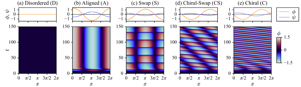
Figure 1: Five characteristic spatiotemporal patterns obtained by numerical simulation. The upper plots show the spatial distribution of $\phi$ (orange) and $\psi$ (purple) at $t=150$. The lower diagrams show the spatiotemporal plot of $\phi$. The reciprocal interaction parameter is fixed to $\chi=1$. (a) Disordered phase (D-phase) when $(\varepsilon,\alpha)=(-1,1.11)$. (b) Aligned phase (A-phase) when $(\varepsilon,\alpha)=(0.5,1.11)$. (c) Swap phase (S-phase) when $(\varepsilon,\alpha)=(0.5,1.13)$. (d) Chiral-swap phase (CS-phase) when $(\varepsilon,\alpha)=(0.5,1.15)$. (e) Chiral phase (C-phase) when $(\varepsilon,\alpha)=(0.5,1.17)$.

III Identification of patterns

We employ Fourier spectra to quantitatively classify the five characteristic spatiotemporal patterns obtained in the numerical results. We limit our discussion to the case of $L=2\pi$ to simplify the analysis. The spatiotemporal Fourier expansion is defined by

$$\phi(t,x)=\sum_{m=-N_{\mathrm{max}}^{(t)}/2}^{N_{\mathrm{max}}^{(t)}/2}\sum_{n=-N_{\mathrm{max}}^{(x)}/2}^{N_{\mathrm{max}}^{(x)}/2}e^{i(m\omega_{0}t-nk_{0}x)}\tilde{\phi}_{m,n},$$ (3)

where $\omega_{0}={2\pi}/{T_{\mathrm{max}}}$ and $k_{0}={2\pi}/{L}=1$. The time evolution was computed up to $T_{\mathrm{max}}=2\times 10^{4}$, and the data for $0\leq t<4\times 10^{3}$ were disregarded. The sampling numbers were $N_{\mathrm{max}}^{(t)}=4\times 10^{4}$ and $N_{\mathrm{max}}^{(x)}=64$.

The Fourier power spectrum $\left|\tilde{\phi}_{m,1}\right|^{2}$ is shown in Figs. 2(a) and (b) for the cases of $\varepsilon=0.5$ and $\varepsilon=1.5$, respectively, with fixed $\chi=1$. As $\alpha$ increases, the behavior of the peak splitting is different between Figs. 2(a) and (b). Hereafter, we denote $\omega=m\omega_{0}$. Because of the spatial inversion symmetry inherent in the 1D NRSH model, the spectrum was reflected with respect to $\omega=0$ if the maximum peak of $\left|\tilde{\phi}_{m,1}\right|^{2}$ was found at $\omega<0$. This procedure guarantees that the maximum peak is located at $\omega\geq 0$. In the following, we discuss in detail the case of Fig. 2(a), where more abundant phases appear, and describe the criteria for determining the spatiotemporal phases.

In the region where $\alpha$ is small, there is only one peak at $\omega=0$, which is defined as the A-phase with a stationary solution. When $\alpha\simeq 1.12$, the spectrum is divided, and peaks appear at both $\omega=\omega_{+}>0$ and $\omega=\omega_{-}<0$. In particular, when $\omega_{+}=-\omega_{-}$ and $\left|\tilde{\phi}_{+}\right|^{2}=\left|\tilde{\phi}_{-}\right|^{2}$, the amplitudes of the leftward and rightward traveling waves are equal, which is defined as the S-phase with a standing wave-like dynamics. In the case $\alpha\gtrsim 1.12$ and $\omega_{+}+\omega_{-}\neq 0$, both traveling wave-like oscillations and amplitude oscillations are observed, which is defined as the CS-phase. For larger $\alpha$, there is only one peak in the region of $\omega>0$. This represents a traveling wave with a stationary waveform, which is defined as the C-phase.

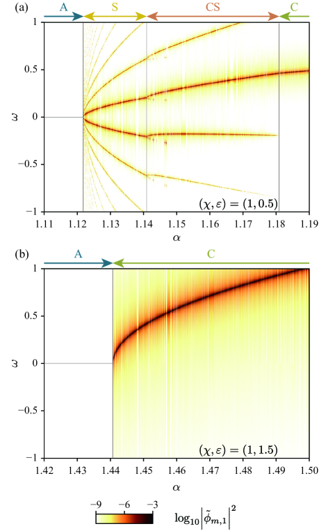
Figure 2: Dependence of Fourier spectra $\left|\tilde{\phi}_{m,1}\right|^{2}$ on $\alpha$. Spectra are reflected with respect to $\omega=0$ if the maximum peak of $\left|\tilde{\phi}_{m,1}\right|^{2}$ is found at $\omega<0$. The corresponding spatiotemporal phases are shown above each spectrum. The parameter is fixed to $\chi=1$. (a) $\varepsilon=0.5$, (b) $\varepsilon=1.5$.

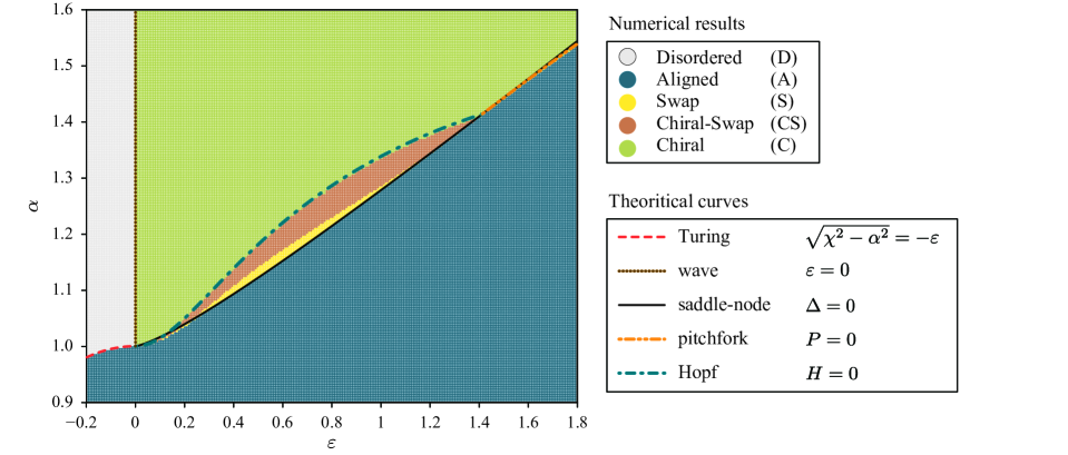
Figure 3: Phase diagram in the $\varepsilon$-$\alpha$ plane when $L=2\pi$ and $\chi=1$. The criteria for each phase are described in Appendix B. The phase diagram obtained from numerical simulation is overlaid with theoretical lines obtained from the analysis of the reduced dynamical system in Sec. IV. The theoretical lines correspond to the Turing bifurcation (red dashed line), wave bifurcation (brown dotted line), saddle-node bifurcation (black solid line), pitchfork bifurcation (orange dash-double-dotted line), and Hopf bifurcation (cyan dash-dotted line).

Figure 3 shows the phase diagram obtained by the above classification when $\chi=1$. The quantitative criteria for determining the phases are described in Appendix B. If we focus on the lower left region of the phase diagram, the A-phase appears even when $\varepsilon<0$ due to the coupling interactions. With an increase in $\varepsilon$, the D-phase changes to the A-phase and C-phase, which are destabilized by Turing and wave bifurcations, respectively.

In the region with positive $\varepsilon$, an increase in $\alpha$ leads to the appearance of the A-phase, S-phase, CS-phase, and C-phase in this order in the range of $0<\varepsilon\lesssim 1.4$, and there is a direct transition from the A-phase to the C-phase in the range of $\varepsilon\gtrsim 1.4$. At the point $\alpha\simeq 1$ and $\varepsilon\simeq 0$ and that with $\alpha\simeq\varepsilon\simeq 1.4$, the boundaries of each phase appear to converge to a single point. The details of bifurcation structures and the derivation of the theoretical lines are discussed in Sec. IV.

IV Theoretical analysis

IV.1 Linear stability analysis

We first perform a linear stability analysis around the D-phase and show that the A-phase and C-phase appear through Turing and wave bifurcations, respectively. We perform the spatial Fourier series expansion to investigate the appearance of patterns with finite wavenumbers. In the following, we consider the dynamics of $\phi(t,x)$ and $\psi(t,x)$ in $0\leq x<L$ with a periodic boundary condition. The Fourier series expansion with respect to $x$ is described as

$$\phi(t,x) =\sum_{n=-\infty}^{\infty}\phi_{n}(t)e^{-ik_{0}nx},$$ (4)

$$\psi(t,x) =\sum_{n=-\infty}^{\infty}\psi_{n}(t)e^{-ik_{0}nx}.$$ (5)

Because both $\phi$ and $\psi$ are real, the Fourier coefficients satisfy the relations $\phi_{n}=\phi^{*}_{-n}$ and $\psi_{n}=\psi^{*}_{-n}$, where ^∗ denotes complex conjugate. By the substitution of Eqs. (4) and (5) into the NRSH model in Eqs. (1) and (2), the ordinary differential equations for the $n$-th mode Fourier components are derived as

$$\dot{\phi}_{n} =\left[\varepsilon-\left(1-k_{0}^{2}n^{2}\right)^{2}\right]\phi_{n}-F_{n}(\{\phi_{m}\})-(\chi+\alpha)\psi_{n},$$ (6)

$$\dot{\psi}_{n} =\left[\varepsilon-\left(1-k_{0}^{2}n^{2}\right)^{2}\right]\psi_{n}-F_{n}(\{\psi_{m}\})-(\chi-\alpha)\phi_{n},$$ (7)

where the third-order nonlinear term $F_{n}$ is defined as

$$F_{n}(\{\phi_{m}\}) =\sum_{m_{1}=-\infty}^{\infty}\sum_{m_{2}=-\infty}^{\infty}\phi_{m_{1}}\phi_{m_{2}}\phi_{n-m_{1}-m_{2}},$$ (8)

$$F_{n}(\{\psi_{m}\}) =\sum_{m_{1}=-\infty}^{\infty}\sum_{m_{2}=-\infty}^{\infty}\psi_{m_{1}}\psi_{m_{2}}\psi_{n-m_{1}-m_{2}}.$$ (9)

Since $n$ takes all integers, Eqs. (6) and (7) represent a coupled system of an infinite number of ordinary differential equations for the Fourier coefficients $\{(\phi_{n},\psi_{n})\}$.

Here, we consider the case with $k_{0}=1$ for simplicity. In this case, the eigenvalues obtained from the linearized equations around the trivial solution $(\phi,\psi)=(0,0)$ are

$$\lambda_{n}^{\pm}=\varepsilon-\left(1-n^{2}\right)^{2}\pm\left(\chi^{2}-\alpha^{2}\right)^{1/2}.$$ (10)

It should be noted that the real part of the eigenvalues is maximized when $n=\pm 1$. When $\alpha\leq\chi$, the instability condition $\lambda_{\pm 1}^{+}>0$ is satisfied if $\sqrt{\chi^{2}-\alpha^{2}}>-\varepsilon$. The boundary line, $\sqrt{\chi^{2}-\alpha^{2}}=-\varepsilon$, is shown in Fig. 3 as the red dashed line. In this case, the eigenvalues do not have the imaginary part, which corresponds to the Turing instability. When $\alpha>\chi$, the real part of $\lambda_{\pm 1}^{+}$ is $\varepsilon$, and thus the D-phase is destabilized when $\varepsilon>0$, leading to the appearance of the C-phase. Moreover, $\lambda_{\pm 1}^{+}$ has an imaginary part $\pm i\sqrt{\alpha^{2}-\chi^{2}}$, which implies the wave instability. The boundary line, $\varepsilon=0$, is shown in Fig. 3 as the brown dotted line.

IV.2 Reduced ordinary differential equation for Fourier coefficients

Next, we consider the dominant unstable modes $n=\pm 1$ and ignore the other modes in the analysis. Under this approximation, the possible three combinations of $(m_{1},m_{2},1-m_{1}-m_{2})$ are $(1,1,-1)$, $(1,-1,1)$, and $(-1,1,1)$ in Eq. (8) and (9) for $n=1$. The resulting expressions for the nonlinear terms $F_{1}(\left\{\phi_{m}\right\})$ and $F_{1}(\{\psi_{m}\})$ are approximated as $3|\phi_{1}|^{2}\phi_{1}$ and $3|\psi_{1}|^{2}\psi_{1}$, respectively. Consequently, we obtain a system of coupled ordinary differential equations for the complex order parameters $\phi_{1}$ and $\psi_{1}$ as

$$\dot{\phi}_{1} =\varepsilon\phi_{1}-3|\phi_{1}|^{2}\phi_{1}-(\chi+\alpha)\psi_{1},$$ (11)

$$\dot{\psi}_{1} =\varepsilon\psi_{1}-3|\psi_{1}|^{2}\psi_{1}-(\chi-\alpha)\phi_{1}.$$ (12)

We further reduce the degrees of freedom by focusing on the phase translational symmetry of Eqs. (11) and (12), which originates from the spatial translational symmetry. We set $\phi_{1}=\rho_{1}e^{i\theta_{1}}$ and $\psi_{1}=\rho_{2}e^{i\theta_{2}}$, where $\rho_{1}$ and $\rho_{2}$ are non-negative real values, while $\theta_{1}$ and $\theta_{2}$ are real values. Furthermore, by defining the phase difference as $\delta=\theta_{2}-\theta_{1}$ and by substituting them into Eqs. (11) and (12), we obtain a three-variable dynamical system as

$$\dot{\rho}_{1} =\varepsilon\rho_{1}-3\rho_{1}^{3}-(\chi+\alpha)\rho_{2}\cos\delta,$$ (13)

$$\dot{\rho}_{2} =\varepsilon\rho_{2}-3\rho_{2}^{3}-(\chi-\alpha)\rho_{1}\cos\delta,$$ (14)

$$\dot{\delta} =\left[(\chi-\alpha)\frac{\rho_{1}}{\rho_{2}}+(\chi+\alpha)\frac{\rho_{2}}{\rho_{1}}\right]\sin\delta.$$ (15)

Note that $\dot{\theta}_{1}$ and $\dot{\theta}_{2}$ obey

$$\dot{\theta}_{1} =-(\chi+\alpha)\frac{\rho_{2}}{\rho_{1}}\sin\delta,$$ (16)

$$\dot{\theta}_{2} =(\chi-\alpha)\frac{\rho_{1}}{\rho_{2}}\sin\delta,$$ (17)

and thus $\dot{\theta}_{1}$ and $\dot{\theta}_{2}$ do not necessarily become zero even if $\dot{\delta}=0$.

IV.3 Fixed points of the reduced system and corresponding spatiotemporal patterns

We consider the fixed points $(\rho_{1}^{(0)},\rho_{2}^{(0)},\delta^{(0)})$ of the reduced three-variable dynamical system in Eqs. (13), (14) and (15) by setting $\dot{\rho}_{1}=\dot{\rho}_{2}=\dot{\delta}=0$. Regarding $\dot{\delta}=0$ in Eq. (15), either $\sin\delta^{(0)}=0$ or $(\chi-\alpha)\rho_{1}^{(0)}/\rho_{2}^{(0)}+(\chi+\alpha)\rho_{2}^{(0)}/\rho_{1}^{(0)}=0$ is necessary. As will be seen in the subsequent analysis, the solutions for the former equation correspond to the A-phase, and the ones for the latter equation correspond to the C-phase.

First, we consider the fixed point with $\sin\delta^{(0)}=0$. We substitute Eq. (13) with $\dot{\rho}_{1}=0$ into Eq. (14) with $\dot{\rho}_{2}=0$ and define $\zeta$ as

$$\zeta=\frac{\varepsilon-3\left(\rho_{1}^{(0)}\right)^{2}}{\chi+\alpha},$$ (18)

where we assume $\chi+\alpha>0$. Then, we obtain a quartic equation of $\zeta$ as 

$$(\chi+\alpha)\zeta^{4}-\varepsilon\zeta^{3}+\varepsilon\zeta-(\chi-\alpha)=0.$$ (19)

The discriminant $\Delta$ of the quartic equation in Eq. (19) is given by

$$\frac{\Delta}{4}={} 64\alpha^{6}-192\alpha^{4}\chi^{2}+48\alpha^{4}\varepsilon^{2}+192\alpha^{2}\chi^{4}-96\alpha^{2}\chi^{2}\varepsilon^{2}$$

$$-15\alpha^{2}\varepsilon^{4}-64\chi^{6}+48\chi^{4}\varepsilon^{2}-12\chi^{2}\varepsilon^{4}+\varepsilon^{6}.$$ (20)

The number of fixed points changes when the sign of $\Delta$ changes. Therefore, $\Delta=0$ gives the saddle-node bifurcation line, shown as the black solid line in Fig. 3. Considering the original spatiotemporal variables, one can recover as $\phi(t,x)=2\rho_{1}^{(0)}\cos(x+\theta_{0})$ and $\psi(t,x)=\pm 2\rho_{2}^{(0)}\cos(x+\theta_{0})$, which correspond to the A-phase. Here $\theta_{0}$ is an arbitrary constant due to the spatial translational symmetry. Moreover, by examining the quartic equation of $\zeta$ in detail, we find that the number of fixed points changes depending on the signs of $\Delta$ and $(\varepsilon/\chi)^{2}+(\alpha/\chi)^{2}-1$. In Fig. 4(a), we show the number of fixed points in the $(\varepsilon/\chi)$-$(\alpha/\chi)$ plane.

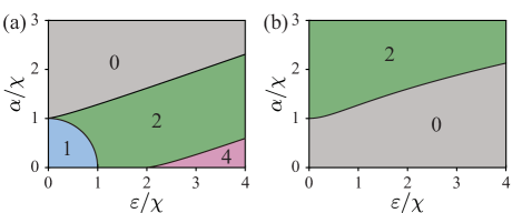
Figure 4: Number of fixed points in the reduced dynamical system. (a) A-phase. (b) C-phase.

Next, we consider the case when $(\chi-\alpha)\rho_{1}^{(0)}/\rho_{2}^{(0)}+(\chi+\alpha)\rho_{2}^{(0)}/\rho_{1}^{(0)}=0$ holds, the other sufficient condition for $\dot{\delta}=0$. In this case, the fixed points are explicitly given by

$$\rho_{1}^{(0)} =\sqrt{\frac{\varepsilon}{3\alpha}(\alpha+\chi)},$$ (21)

$$\rho_{2}^{(0)} =\sqrt{\frac{\varepsilon}{3\alpha}(\alpha-\chi)},$$ (22)

$$\cos\delta^{(0)} =-\frac{\chi\varepsilon}{\alpha\sqrt{\alpha^{2}-\chi^{2}}}.$$ (23)

The existence of this fixed point is equivalent to the condition that $\varepsilon>0$, $\alpha>\chi$, and $P\geq 0$, where $P$ is defined as

$$P=\alpha^{4}-\alpha^{2}\chi^{2}-\chi^{2}\varepsilon^{2}.$$ (24)

As shown in the next subsection, the boundary line $P=0$ corresponds to the pitchfork bifurcation, which is shown in Fig. 3 as the orange dash-double-dotted line. The fixed point in the reduced three-variable dynamical system corresponds to the solution $\dot{\theta}_{1}=\dot{\theta}_{2}$ for the four-variable dynamical system. Here,

$$\left|\dot{\theta}_{1}\right|=\left|\dot{\theta}_{2}\right|=\frac{\sqrt{P}}{\alpha}=\sqrt{\alpha^{2}-\chi^{2}-\frac{\chi^{2}\varepsilon^{2}}{\alpha^{2}}},$$ (25)

where the signs of $\dot{\theta}_{1}$ and $\dot{\theta}_{2}$ indicate the direction of wave propagation in the real space. Therefore, $\phi(t,x)$ and $\psi(t,x)$ propagate with a constant phase difference of $\delta^{(0)}$ at a phase velocity $\Omega_{0}=\sqrt{P}/\alpha$ in the original spatiotemporal variables, $\phi(t,x)=2\rho_{1}^{(0)}\cos(x\mp\Omega_{0}t+\theta_{1}^{(0)})$ and $\psi(t,x)=2\rho_{2}^{(0)}\cos(x\mp\Omega_{0}t+\theta_{1}^{(0)}+\delta^{(0)})$, which corresponds to the C-phase. The different signs represent rightward and leftward propagating waves.

In Fig. 4(b), we show the number of fixed points for the C-phase in the $(\alpha/\chi)$-$(\varepsilon/\chi)$ plane. The stability condition for the fixed points for the C-phase is derived by using the Routh-Hurwitz stability criterion [32]:

$$H=\alpha^{4}-\alpha^{2}\chi^{2}+2\alpha^{2}\varepsilon^{2}-5\chi^{2}\varepsilon^{2}>0.$$ (26)

Upon examining the eigenvalues of the Jacobi matrix around the fixed point for the C-phase on the boundary line $H=0$, we obtain one negative eigenvalue and two purely imaginary eigenvalues. This suggests that the boundary $H=0$ corresponds to the Hopf bifurcation line, which is shown in Fig. 3 as the cyan dash-dotted line.

IV.4 Connection of branches and bifurcation structures

In the previous sections, we investigated the existence and stability conditions in the reduced dynamical system for the spatial Fourier modes obtained from the NRSH model. The fixed points for the A-phase and C-phase are obtained from the conditions $\sin\delta^{(0)}=0$ and $(\chi-\alpha)\rho_{1}^{(0)}/\rho_{2}^{(0)}+(\chi+\alpha)\rho_{2}^{(0)}/\rho_{1}^{(0)}=0$, respectively. The fixed points for the C-phase also satisfy $\sin\delta^{(0)}=0$ if $P=0$, leading to an intersection of the branches of the A-phase and C-phase at a pitchfork bifurcation point. The bifurcation structure depends on the ratio $\varepsilon/\chi$, as schematically shown in Figs. 5(a) and (b).

When $\varepsilon/\chi<\sqrt{2}$ in Fig. 5(a), there are three characteristic values of $\alpha$: the pitchfork bifurcation point $\alpha_{\mathrm{PF}}$, the saddle-node bifurcation point $\alpha_{\mathrm{SN}}$, and the Hopf bifurcation point $\alpha_{\mathrm{HB}}$, where $\alpha_{\mathrm{PF}}<\alpha_{\mathrm{SN}}<\alpha_{\mathrm{HB}}$. These points are characterized by $P=0$, $\Delta=0$, and $H=0$, respectively. For $0\leq\alpha<\alpha_{\mathrm{PF}}$, there are two fixed points for the A-phase, where one is stable and the other is unstable. At the pitchfork bifurcation point $\alpha=\alpha_{\mathrm{PF}}$, two unstable fixed points for the C-phase emerge from the unstable fixed point for the A-phase. Note that the value of $\delta^{(0)}$ for the fixed points corresponding to the C-phase are symmetric with respect to $\pi$, reflecting the symmetry of $\cos\delta$ around $\delta=\pi$. Considering this, for $\alpha_{\mathrm{PF}}<\alpha<\alpha_{\mathrm{SN}}$, there are four fixed points; two of which are stable and unstable fixed points for the A-phase, and the other two are unstable fixed points for the C-phase. At the saddle-node bifurcation point $\alpha=\alpha_{\mathrm{SN}}$, the stable and unstable fixed points for the A-phase merge and disappear. For $\alpha_{\mathrm{SN}}<\alpha<\alpha_{\mathrm{HB}}$, there are two fixed points, both of which are unstable, corresponding to the C-phase. At the Hopf bifurcation point $\alpha=\alpha_{\mathrm{HB}}$, the two fixed points for the C-phase change stability; they are stable for $\alpha>\alpha_{\mathrm{HB}}$ and unstable for $\alpha<\alpha_{\mathrm{HB}}$. Moreover, for $\alpha<\alpha_{\mathrm{HB}}$, two stable closed orbits, which correspond to the CS-phase, are generated from each Hopf bifurcation point. For $\alpha>\alpha_{\mathrm{HB}}$, there are two fixed points for the C-phase, both of which are stable.

When $\varepsilon/\chi>\sqrt{2}$ in Fig. 5(b), there are two characteristic values of $\alpha$; the pitchfork bifurcation point $\alpha_{\mathrm{PF}}$ and the saddle-node bifurcation point $\alpha_{\mathrm{SN}}$, where $\alpha_{\mathrm{PF}}<\alpha_{\mathrm{SN}}$. For $\alpha<\alpha_{\mathrm{PF}}$, there are two fixed points for the A-phase, one of which is stable and the other is unstable. At the pitchfork bifurcation point $\alpha=\alpha_{\mathrm{PF}}$, two stable fixed points corresponding to the C-phase are generated from the stable fixed point corresponding to the A-phase. By this pitchfork bifurcation, the stable fixed point for the A-phase becomes unstable, and both fixed points corresponding to the A-phase are unstable for $\alpha_{\mathrm{PF}}<\alpha<\alpha_{\mathrm{SN}}$. For $\alpha_{\mathrm{PF}}<\alpha<\alpha_{\mathrm{SN}}$, there are four fixed points; two of which are unstable fixed points corresponding to the A-phase, and the other two are stable fixed points for the C-phase. At the saddle-node bifurcation point $\alpha=\alpha_{\mathrm{SN}}$, the stable and unstable fixed points for the A-phase merge and disappear. For $\alpha>\alpha_{\mathrm{SN}}$, there are two fixed points corresponding to the C-phase, both of which are stable.

When $\varepsilon/\chi=\sqrt{2}$, the pitchfork, saddle-node, and Hopf bifurcations degenerate at $\alpha_{\mathrm{PF}}=\alpha_{\mathrm{SN}}=\alpha_{\mathrm{HB}}=\sqrt{2}\chi$, suggesting a high-codimensional bifurcation at this point. Similarly, at the point $\alpha/\chi=1$ and $\varepsilon/\chi=0$, the wave bifurcation point and the Turing bifurcation point coincide. Analyses of these higher-codimensional bifurcations are left for future work.

According to the numerical calculations of the reduced dynamical system, the S-phase appears from the A-phase by a global bifurcation. For example, when $\varepsilon/\chi$ is slightly less than $\sqrt{2}$, a periodic orbit corresponding to the S-phase emerges due to an infinite period bifurcation when the fixed points for the A-phase disappear due to a saddle-node bifurcation. Furthermore, when $\varepsilon/\chi$ is small, the S-phase is suggested to appear through a homoclinic bifurcation around the unstable fixed points for the A-phase. The details of these global bifurcations are also left for future research.

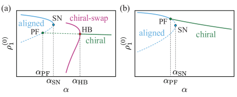
Figure 5: Schematic diagrams of the bifurcation structure of the fixed points for the A-phase (blue line) and C-phase (green line). The maximum and minimum values of the periodic orbits corresponding to the CS-phase generated by the Hopf bifurcation are shown by the magenta line. Solid and dashed lines represent stable and unstable fixed points, respectively. (a) $\varepsilon/\chi<\sqrt{2}$, (b) $\varepsilon/\chi>\sqrt{2}$. PF: pitchfork bifurcation point, SN: saddle-node bifurcation point, HB: Hopf bifurcation point.

V Discussion

Several studies have been reported on the 1D complex SH equation [33, 34, 35, 36]. The typical form of the complex SH equation is written as

$$\dot{w}=\left[c_{1}-c_{2}\left(1+\partial_{x}^{2}\right)^{2}\right]w-c_{3}|w|^{2}w,$$ (27)

where $w$ is a complex order parameter, and $c_{1}$, $c_{2}$, and $c_{3}$ are complex parameters. The complex SH equation no longer has gradient dynamics when the parameters $c_{1}$, $c_{2}$, and $c_{3}$ are complex. There are reports of traveling wave patterns similar to those in the 1D NRSH model [33, 35]. However, in the complex SH equation with translational symmetry of the phase factor for $w$, the interactions corresponding to the reciprocal interactions $-\chi\psi$ and $-\chi\phi$ in the NRSH model cannot be represented even if the coefficients are complex. Although solutions for the A-phase and C-phase appear in the complex SH equation, patterns with amplitude oscillations, such as the S-phase and CS-phase, do not appear. Reciprocal interactions break the translational symmetry of the phase factor of $w$ and can generate patterns with amplitude oscillations. To express reciprocal interactions in the complex SH equation, it is necessary to introduce terms that break the translational symmetry of the phase factor, such as $-i\chi w^{*}$ in the time evolution of $w$.

In the 2D complex SH equation, traveling domain wall structures and spiral structures were observed [37]. Recently, an experimental study reported self-integrated atomic quantum wires and junctions of a Mott semiconductor [38]. These studies revealed the emergence of unique spiral patterns in reaction-diffusion systems. To provide a theoretical analysis of these observations, a model using the 2D complex SH equation was employed. The numerical calculations demonstrated the generation and progression of stripe patterns originating from the initial spiral structure. The stripe patterns that propagate with a finite characteristic wavenumber correspond to the C-phase in our 1D NRSH model. In 2D systems, topological defects appear, and the spatiotemporal pattern dynamics become more complex.

In the 1D NRSH model, we derived the reduced model by focusing on the Fourier modes around the characteristic wavenumber. Here, we discuss the relationship between the 1D NRSH model and the 1D NRCH model. In the 1D NRCH model, amplitude equations can be obtained by a reduction around the characteristic wavenumber [9]. By considering the 0th Fourier mode as an appropriate parameter, a set of amplitude equations that is completely equivalent to that in the NRSH model can be obtained. This suggests that the spatiotemporal pattern dynamics of the NRSH and NRCH models are equivalent when the system size is sufficiently small, and only the modes around the characteristic wavenumber play an essential role.

Differences between the NRSH and NRCH models are expected to appear through the coupling with other wavenumber modes, such as the presence or absence of oscillations in the 0th Fourier mode and long-wavelength instabilities known as the Eckhaus instability [39], or in the systems with spatial dimension of two or more. When numerical calculations were performed on the NRSH model with a large system size $L=48\pi$, long-wavelength instabilities were observed as shown in Fig. 6. The spatial pattern of the S-phase slips to the left and right due to the coupling with long-wavelength modes, similar to the CS-phase. In the CS-phase and C-phase, sinks and sources appear, and the advancing waves move towards or away from them.

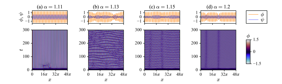
Figure 6: Characteristic spatiotemporal patterns observed in numerical simulation in the 1D NRSH model with $L=48\pi$. The upper plots show the spatial distribution of $\phi$ and $\psi$ at $t=300$, where orange and purple lines represent $\phi$ and $\psi$, respectively. The lower diagrams show the spatiotemporal plot of $\phi$. The non-reciprocal interaction parameter $\alpha$ in each phase is varied. (a) $\alpha=1.11$, (b) $\alpha=1.13$, (c) $\alpha=1.15$, and (d) $\alpha=1.2$. The other parameters are fixed at $\varepsilon=0.5$ and $\chi=1$.

VI Conclusion

In this study, we have investigated the pattern dynamics and phase transitions of the 1D NRSH model through numerical calculations and theoretical analyses. Numerical simulations revealed that the spatially periodic wave (A-phase) appears when non-reciprocity $\alpha$ is sufficiently small, while the traveling wave with a constant amplitude (C-phase) appears when $\alpha$ is large. Depending on the reciprocity $\chi$ and the destabilization parameter $\varepsilon$, the S-phase and CS-phase appear. By considering the Fourier modes corresponding to the characteristic wavenumber, we derived a reduced low-dimensional dynamical system. Our theoretical analyses clarified the bifurcation structure of the reduced system, particularly the fixed points corresponding to the A-phase and C-phase. The results of our analyses provide insights into the phase diagram obtained by the numerical classification of the spatiotemporal Fourier spectrum. Our findings underscore the unique characteristics of non-reciprocal continuum systems, where transitions to dynamic phases are driven by non-reciprocity. We also unveiled the rich bifurcation structure including S-phase and CS-phase, which is likely due to the presence of both reciprocal and non-reciprocal interactions. More detailed analyses for them are necessary to achieve a deeper understanding of the non-reciprocal continuum dynamics.

Appendix A Numerical scheme

We describe the numerical scheme. The spatial grid size was $\Delta x=L/N\simeq 0.05$. The initial condition $(\phi_{0},\psi_{0})$ was set by the Gaussian white noise with zero mean and variance $0.1$ at each spatial point. The 1D Laplace operator $\partial_{x}^{2}$ was approximated with second-order accuracy using a central difference scheme, and the time evolution was performed using an open-source differential equation solver employing the explicit singly diagonal implicit Runge-Kutta (ESDIRK) method [40].

Appendix B Criteria for determining the phases

We defined the criteria for determining the D-phase, A-phase, S-phase, CS-phase, and C-phase. We focused on the Fourier component ${\tilde{\phi}}_{m,1}$ of $\phi(t,x)$. If the maximum value of $\left|{\tilde{\phi}}_{m,1}\right|^{2}$ as a function of $\omega$ was less than $10^{-4}$, it was determined to be the D-phase. If the maximum value of $\left|{\tilde{\phi}}_{m,1}\right|^{2}$ with respect to $\omega$ was given at $\omega=0$, it was determined to be the A-phase. In case the maximum value was given at $\omega\neq 0$, if there was only one maximum value of $\left|{\tilde{\phi}}_{m,1}\right|^{2}$ with respect to $\omega$, or the ratio of the maximum value of $\left|{\tilde{\phi}}_{m,1}\right|^{2}$ to the next largest value of $\left|{\tilde{\phi}}_{m,1}\right|^{2}$ was less than $10^{-2}$, it was determined to be the C-phase. Let $\omega_{1}$ and $\omega_{2}$ be the frequencies of the maximum and the next largest values of $\left|{\tilde{\phi}}_{m,1}\right|^{2}$, respectively. If $|\omega_{1}+\omega_{2}|$ was less than $10^{-3}$ and the difference between the maximum value of $\left|{\tilde{\phi}}_{m,1}\right|^{2}$ and the next largest value was less than $10^{-2}$, it was determined to be the S-phase. Otherwise, it was determined to be the CS-phase.

References

- Fruchart et al. [2021] M. Fruchart, R. Hanai, P. B. Littlewood, and V. Vitelli, “Non-reciprocal phase transitions,” Nature 592, 363 (2021).
- Ivlev et al. [2015] A. V. Ivlev, J. Bartnick, M. Heinen, C.-R. Du, V. Nosenko, and H. Löwen, “Statistical mechanics where Newton’s third law is broken,” Phys. Rev. X 5, 011035 (2015).
- Ishikawa et al. [2022] H. Ishikawa, Y. Koyano, H. Kitahata, and Y. Sumino, “Pairing-induced motion of source and inert particles driven by surface tension,” Phys. Rev. E 106, 024604 (2022).
- Theveneau et al. [2013] E. Theveneau, B. Steventon, E. Scarpa, S. Garcia, X. Trepat, A. Streit, and R. Mayor, “Chase-and-run between adjacent cell populations promotes directional collective migration,” Nat. Cell Biol. 15, 763 (2013).
- Agudo-Canalejo and Golestanian [2019] J. Agudo-Canalejo and R. Golestanian, “Active phase separation in mixtures of chemically interacting particles,” Phys. Rev. Lett. 123, 018101 (2019).
- Zhang et al. [2021] J. Zhang, R. Alert, J. Yan, N. S. Wingreen, and S. Granick, “Active phase separation by turning towards regions of higher density,” Nat. Phys. 17, 961 (2021).
- Wittkowski et al. [2014] R. Wittkowski, A. Tiribocchi, J. Stenhammar, R. J. Allen, D. Marenduzzo, and M. E. Cates, “Scalar field theory for active-particle phase separation,” Nat. Commun. 5, 4351 (2014).
- Kant et al. [2024] R. Kant, R. K. Gupta, H. Soni, A. Sood, and S. Ramaswamy, “Bulk condensation by an active interface,” arXiv:2403.18329 (2024).
- You et al. [2020] Z. You, A. Baskaran, and M. C. Marchetti, “Nonreciprocity as a generic route to traveling states,” Proc. Natl. Acad. Sci. USA 117, 19767 (2020).
- Saha et al. [2020] S. Saha, J. Agudo-Canalejo, and R. Golestanian, “Scalar active mixtures: The nonreciprocal Cahn-Hilliard model,” Phys. Rev. X 10, 041009 (2020).
- Frohoff-Hülsmann et al. [2023] T. Frohoff-Hülsmann, M. P. Holl, E. Knobloch, S. V. Gurevich, and U. Thiele, “Stationary broken parity states in active matter models,” Phys. Rev. E 107, 064210 (2023).
- Allen and Cahn [1979] S. M. Allen and J. W. Cahn, “A microscopic theory for antiphase boundary motion and its application to antiphase domain coarsening,” Acta Metall. 27, 1085 (1979).
- Cahn and Hilliard [1958] J. W. Cahn and J. E. Hilliard, “Free energy of a nonuniform system. I. Interfacial free energy,” J. Chem. Phys. 28, 258 (1958).
- Thiele et al. [2016] U. Thiele, A. J. Archer, and L. M. Pismen, “Gradient dynamics models for liquid films with soluble surfactant,” Phys. Rev. Fluids 1, 083903 (2016).
- Liu et al. [2023] M. Liu, Z. Hou, H. Kitahata, L. He, and S. Komura, “Non-reciprocal phase separations with non-conserved order parameters,” J. Phys. Soc. Jpn. 92, 093001 (2023).
- Saha [2024] S. Saha, “Phase coexistence in the Non-reciprocal Cahn-Hilliard model,” arXiv:2402.10057 (2024).
- Rana and Golestanian [2023] N. Rana and R. Golestanian, “Defect Solutions of the Non-reciprocal Cahn-Hilliard Model: Spirals and Targets,” arXiv:2306.03513 (2023).
- Frohoff-Hülsmann et al. [2021] T. Frohoff-Hülsmann, J. Wrembel, and U. Thiele, “Suppression of coarsening and emergence of oscillatory behavior in a Cahn-Hilliard model with nonvariational coupling,” Phys. Rev. E 103, 042602 (2021).
- Frohoff-Hülsmann and Thiele [2023] T. Frohoff-Hülsmann and U. Thiele, “Nonreciprocal Cahn-Hilliard model emerges as a universal amplitude equation,” Phys. Rev. Lett. 131, 107201 (2023).
- Saha and Golestanian [2022] S. Saha and R. Golestanian, “Effervescent waves in a binary mixture with non-reciprocal couplings,” arXiv:2208.14985 (2022).
- Suchanek et al. [2023] T. Suchanek, K. Kroy, and S. A. M. Loos, “Entropy production in the nonreciprocal cahn-hilliard model,” Phys. Rev. E 108, 064610 (2023).
- Greve et al. [2024] D. Greve, G. Lovato, T. Frohoff-Hülsmann, and U. Thiele, “Maxwell construction for a nonreciprocal Cahn-Hilliard model,” arXiv:2402.08634 (2024).
- Frohoff-Hülsmann and Thiele [2021] T. Frohoff-Hülsmann and U. Thiele, “Localized states in coupled Cahn-Hilliard equations,” IMA J. Appl. Math. 86, 924 (2021).
- Frohoff-Hülsmann et al. [2021] T. Frohoff-Hülsmann, J. Wrembel, and U. Thiele, “Suppression of coarsening and emergence of oscillatory behavior in a Cahn-Hilliard model with nonvariational coupling,” Phys. Rev. E 103, 042602 (2021).
- Brauns and Marchetti [2024] F. Brauns and M. C. Marchetti, “Nonreciprocal pattern formation of conserved fields,” Phys. Rev. X 14, 021014 (2024).
- Swift and Hohenberg [1977] J. Swift and P. C. Hohenberg, “Hydrodynamic fluctuations at the convective instability,” Phys. Rev. A 15, 319 (1977).
- Cross and Hohenberg [1993] M. C. Cross and P. C. Hohenberg, “Pattern formation outside of equilibrium,” Rev. Mod. Phys. 65, 851 (1993).
- Schüler et al. [2014] D. Schüler, S. Alonso, A. Torcini, and M. Bär, “Spatio-temporal dynamics induced by competing instabilities in two asymmetrically coupled nonlinear evolution equations,” Chaos 24 (2014).
- Becker et al. [2018] M. Becker, T. Frenzel, T. Niedermayer, S. Reichelt, A. Mielke, and M. Bär, “Local control of globally competing patterns in coupled Swift–Hohenberg equations,” Chaos 28 (2018).
- Note [1] If is a solution, is also a solution. If the sign of is changed, the equation becomes equivalent by exchanging and . In addition, if the sign of is changed, the equation becomes equivalent by exchanging and . Due to these symmetries, it is sufficient to consider only the region with and .
- Note [2] corresponds to the solution if and only if holds. , , and should have following relations: and when , and when . The case where and is the only case where the phase factor of is undefined, and this occurs only when . When , and , that is, and are fixed points. In this case, . Therefore, it is not the D-phase, and the phase difference cannot be defined because is zero. Such a singularity is known as an exceptional point.
- Gradshteyn and Ryzhik [2014] I. S. Gradshteyn and I. M. Ryzhik, Table of integrals, series, and products (Academic press, 2014).
- Sakaguchi [1997] H. Sakaguchi, “Standing wave patterns for the complex Swift-Hohenberg equation,” Prog. Theor. Exp. Phys. 98, 577 (1997).
- Sakaguchi and Brand [1998] H. Sakaguchi and H. R. Brand, “Localized patterns for the quintic complex Swift-Hohenberg equation,” Physica D: Nonlinear Phenomena 117, 95 (1998).
- Gelens and Knobloch [2011] L. Gelens and E. Knobloch, “Traveling waves and defects in the complex Swift-Hohenberg equation,” Phys. Rev. E 84, 056203 (2011).
- Khairudin et al. [2016] N. Khairudin, F. Abdullah, and Y. Hassan, “Stability of the fixed points of the complex Swift-Hohenberg equation,” in J. Phys. Conf. Ser., Vol. 693 (IOP Publishing, 2016) p. 012003.
- Aranson and Tsimring [1995] I. Aranson and L. Tsimring, “Domain walls in wave patterns,” Phys. Rev. Lett. 75, 3273 (1995).
- Asaba et al. [2023] T. Asaba, L. Peng, T. Ono, S. Akutagawa, I. Tanaka, H. Murayama, S. Suetsugu, A. Razpopov, Y. Kasahara, T. Terashima, Y. Kohsaka, T. Shibauchi, M. Ichikawa, R. Valentí, S.-i. Sasa, and Y. Matsuda, “Growth of self-integrated atomic quantum wires and junctions of a Mott semiconductor,” Sci. Adv. 9, eabq5561 (2023).
- Nishiura [2002] Y. Nishiura, Far-from-equilibrium Dynamics, Vol. 209 (American Mathematical Soc., 2002).
- Rackauckas and Nie [2017] C. Rackauckas and Q. Nie, “DifferentialEquations.jl–a performant and feature-rich ecosystem for solving differential equations in Julia,” J. Open Source Softw. 5 (2017).