Transition magnetic moment about neutrinos
Abstract
This paper investigates the neutrino transition magnetic moment in the SSM. SSM is the extension of Minimal Supersymmetric Standard Model (MSSM) and its local gauge group is extended to . To obtain this model, three singlet new Higgs superfields and right-handed neutrinos are added to the MSSM, which can explain the results of neutrino oscillation experiments. The neutrino transition magnetic moment is induced by electroweak radiative corrections. By applying effective Lagrangian method and on-shell scheme, we study the associated Feynman diagrams and the transition magnetic moment of neutrinos in the model. We fit experimental data for neutrino mass variances and mixing angle. Based on the range of data selection, the influences of different sensitive parameters on the results are analysed. The numerical analysis shows that many parameters have an effect on the neutrino transition moment, such as , , and . For our numerical results, the order of magnitude of is between and .
I Introduction
The Standard Model (SM) comes under the umbrella of quantum field theory, which unifies the three main forces, the strong force, the weak force, and the electromagnetic forceb0 ; b1 ; b2 ; b3 . Although the SM has been a great success, its flaws are obvious. It doesn’t explain the mass problem of neutrinos, the related issue of dark matter, and can’t describe gravityn0 ; n1 ; n2 . Therefore it must be extended. Scientists have made many extensions to the SM, among which the Minimal Supersymmetric Standard Model(MSSM) is a popular one. However, there are problems in MSSM such as the problem31 and zero mass neutrinos32 . To break through these problems, we use the SSMsm2 , that is the extension of the MSSM with the gauge group, and the symmetry group is 7 ; 71 ; 72 .
SSM is formed on the basis of the MSSM by the extension of the local gauge group and its local gauge group is extended to 8 ; 9 . To obtain this model, three Higgs singlet superfields and right-handed neutrino superfield are added to the MSSM, which can explain the results of neutrino oscillation experiments11 . Under SSM, the transition magnetic moment of neutrinos is induced by electroweak radiative corrections. There are some studies of neutrino transport magnetic moments. Such as computing the effects of nonzero Majorana neutrino transition magnetic moments on the oscillation of supernova neutrinos111 or explaining the excess electron recoil events by neutrino transition magnetic moments112 . Besides, it is of great importance in the long distance propagation of neutrinos in the magnetic fields of matter and vacuum12 , and therefore it is necessary to study it.
The study of transition magnetic moment about neutrino using the effective Lagrangian method and the mass-shell scheme has been carried out in previous studies13 . This method can give reasonable numerical results. In this paper, a more comprehensive study of the neutrino transition magnetic moment at the SSM is presented. We obtain an expression for the neutrino transport magnetic moment by the effective Lagrangian method and the mass-shell scheme. We derive the relevant Feynman diagrams and calculate the neutrino transition moment by combining the operators. In the numerical calculation, based on the parameter ranges limited by the experiment, we make the mixing angles. We compare the effect of different reasonable parameters on transition magnetic moment. From the results, the order of magnitude is reasonable.
The paper is organized according to the following structure. In Sec.II, we mainly introduce the content of the SSM including its superpotential, the general soft breaking terms, the mass matrices and couplings. In Sec.III, we give the analytical expressions of the transition magnetic moment about neutrino. In Sec.IV, we give the relevant parameters and numerical analysis. In Sec.V, we present a summary of this article.
II The essential content of SSM
SSM is the extension of MSSM and the local gauge group is . SSM has new superfields, which include three Higgs singlets , and right-handed neutrinos . The corresponding superpotential of the SSM is given by:
| (1) |
The two Higgs doublets and three Higgs singlets can be listed as follows:
| (6) | |||
| (7) |
And the vacuum expectation values of the states , , are respectively ,, and . There are two angles defined as and . The soft SUSY breaking terms of SSM are shown as:
| (8) |
represent the soft breaking terms of MSSM.
| Superfields | |||||||||||
| 3 | 1 | 1 | 1 | 1 | 1 | 1 | 1 | 1 | |||
| 2 | 1 | 1 | 2 | 1 | 1 | 2 | 2 | 1 | 1 | 1 | |
| 1/6 | -2/3 | 1/3 | -1/2 | 1 | 0 | 1/2 | -1/2 | 0 | 0 | 0 | |
| 0 | -1/2 | 1/2 | 0 | 1/2 | -1/2 | 1/2 | -1/2 | -1 | 1 | 0 |
Particle content and charge assignments for SSM are mentioned in the table 1. In our previous work, we have proven that SSM is anomaly free UU3 .
The covariant derivatives of SSM can be written as
| (14) |
Compared with MSSM, SSM has a new effect called the gauge kinetic mixing, which produced by Abelian groups and . The basis conversion occurs when we use the rotation matrix (), which is due to the fact that the two Abelian gauge groups are uninterrupted. The basis conversion can be described by UMSSM5 ; B-L1 ; B-L2 ; gaugemass
| (20) |
with and respectively representing the gauge fields of and . Eq. (20) can be reduced to UMSSM5 ; B-L2 ; gaugemass
| (29) |
Here expresses the gauge coupling constant of the group and expresses the mixing gauge coupling constant of the and groups.
Some useful mass matrices will be listed. The mass matrix for chargino reads:
| (32) |
This matrix is diagonalized by and :
| (33) |
with
| (34) |
The mass matrix for slepton reads:
| (37) |
| (38) | |||||
| (39) | |||||
This matrix is diagonalized by :
| (40) |
with
The mass matrix for neutrino reads:
| (44) |
This matrix diagonalized by :
| (45) |
with
Here, we show some needed couplings in this model. We derive the vertices of --
| (47) |
III formulation
The magnetic dipole moment (MDM) and electric dipole moment (EDM) of the neutrino can be actually be written as the operators
| (48) |
where is the electromagnetic field strength, , denote the four-component Dirac fermions, and are respectively Dirac diagonal () or transition () MDM and EDM between states and .
Since for on-shell fermion and for photon, we can conveniently obtain the contribution of the loop diagram to the fermionic diagonal or leptonic MDM and EDM using the effective Lagrangian method. Then we can expand the amplitude of corresponding triangle diagrams based on the external momenta of fermion and photon. After matching the effective and the holonomic theories, we obtain all high-dimension operators along with their coefficients. We only need to keep those dimension 6 operators for later calculations.
| (49) |
where , , , and is the mass of fermion . The effective vertices with one external photon are written as
| (50) |
By applying the equations of motion to the outer fermions, we obtain the transformation term of the correlation term in the effective LagrangianFeng :
| (51) |
Compared with Eq. (48) and Eq. (51), we can obtain
| (52) |
where, and are the real and imaginary parts of the complex numbers respectively. and is the electron mass.
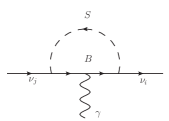
Then we research the processes about the transition magnetic moment of neutrino under the SSM model. The amplitude of can be obtained from the following Feynman diagrams, which are shown in Fig.1.
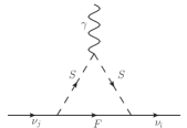
After calculating the left one in Fig.(1) and connecting with Eq.(50), we can get
| (53) |
where is the injecting lepton momentum, is the photon momentum, corresponds to the chargino mass, corresponds to the scalar neutrino (CP-even or CP-odd) mass. and are the wave functions for the external leptons. , and are
| (54) |
At last, we simplify Eq.(53) and use some math calculation software to get the numerical results.
IV Numerical analysis
In this section of the numerical results, we consider some constraints from experiments, which include:
1. The lightest CP-even Higgs mass is around 125.1 GeV. The Higgs decays () can well meet the latest experimental constraints18 ; su1 ; su2 .
2. The constraints from neutrino experiment data including mixing angles and mass variances are considered18 .
3. The boson mass is larger than 5.1 TeV. The ratio between and its gauge 20 .
4. The neutralino mass is limited to more than 116 GeV, and the chargino mass is limited to more than 1000 GeV. The slepton mass is limited to more than 600 GeV 18 .
In meeting the above experimental constraints, we adopt the following parameters in the numerical calculation.
| (55) |
In the following numerical analysis, the parameters to be studied include:
| (56) |
Without special statement, the non-diagonal elements of the parameters are supposed as zero.
IV.1 Neutrino Mixing
In this subsection, by using the top down approach we can derive the formulae for the neutrino mass and mixing angle from the effective neutrino mass matrix. The specifics can be found in the referencesn16 .
The constraints from neutrino experiment data are18
| (57) |
To fit the data of neutrino physics, we take the parameters as
| (58) |
In Fig.2, the constraints from two mass variances are satisfied. Then , and 10 are plotted as dependent variables as changes.
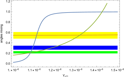
With , , the blue, yellow and green regions correspond to the values of the , and 10 mixing angles in the range, respectively. The blue line represents . It grows consistently from to , with rapid growth from to , but remains almost constant in the region . The yellow line represents . We can find that it goes from to almost unchanged, which is always in the range of . The green line represents 10. With the increase of , the 10 grows faster and faster. From that all, we can see that in order to satisfy the mixing angle from the experiments, the should be one of the values in the range from to .
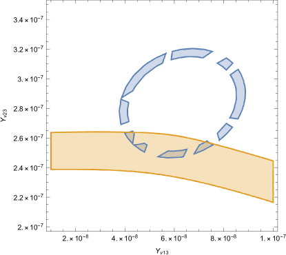
In Fig.3, and are plotted in the plane of versus . With , the constraints from two mass variances and the mixing angle are satisfied(They all in the range of ). The yellow area and blue area represent and respectively. The yellow area looks like a rectangle and blue area looks like a broken ribbon. We can see that where the two regions overlap are the values of and that satisfy the constraints of the two mixing angles. Similarly, in Fig.4 the three constraints from the mixing angles are satisfied(They all in the range of ). and are plotted in the plane of versus . The yellow area represents , which looks like a rectangle. The blue area represents , which looks like a broken bangle. All in all the overlapping part is needed.

IV.2 The processes of
In this part, the objective of this study is to investigate the influence of certain sensitive parameters on the under experimentally constrained conditions. We choose a number of parameters and investigate them to the extent allowed, such as , , , .


We plot and in the Fig.5 (a), in which the dashed line corresponds to = 0.3 and the solid line corresponds to = 0.1. Here, we take = 1000 GeV and = 1200 GeV. We find that the both lines increase first then decrease later with increasing in the range of 0.3-0.51. And the solid line is larger than the dashed line. In Fig.5 (b), with = 0.5(dashed line), = 0.3(solid line), we take = 0.1 and = 1200 GeV. As solid and dashed lines go from bottom to top, increases as increases. They are decreasing functions of . In Fig.5 (c), we take = 1000 GeV and = 0.3. The solid and dashed lines respectively represent GeV and GeV. Both the dashed and solid lines are decreasing functions as turns large. In Fig.5 (d), we take = 0.1 and =0.3. The solid and dashed lines represent GeV and GeV respectively. From the graph, both of them are decreasing functions. When the horizontal coordinates are the same, the slope of the solid line is greater than the dashed line.
From the above graph we conclude that increases with and decreases with , and . The order of magnitude of the change in induced by a 0.1 change in the values of and is similar to that induced by a 100 change in the values of and . So and are more sensitive than and . Overall, , , and are indeed sensitive parameters that have great impacts on .
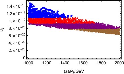
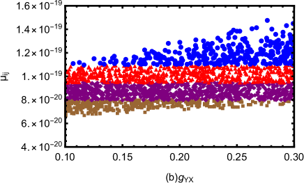
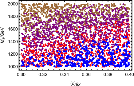
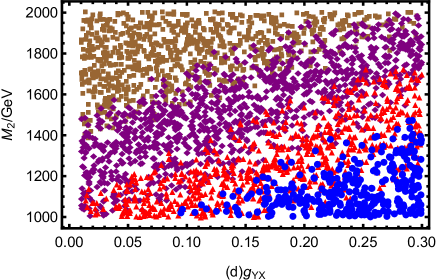
To explore the parameter spaces well, we create scatter diagrams for specific parameters shown in Fig.6. The parameters are listed in TABLE 2. Then, we use to represent the results of the transition magnetic moment.
| Parameters | |||
|---|---|---|---|
| Min | 0.3 | 0.01 | 1000 |
| Max | 0.4 | 0.3 | 2000 |
In Fig.6(a), we made scatter plots of versus . The overall figure resembles a parallelogram. We can see that is at the top, and are in the middle and is on top of . Finally is at the bottom. It can be seen that decreases as increases.
In Fig.6(b), we made scatter plots of versus . It has the same graphic color layout as Fig.6(a), just with a different trend. It can be gotten that the value of increases as increases.
Fig.6(c) shows the effects of and on . Viewed from the whole, different values of in the parameter space are stratified. The upper left corner of these is , followed by , immediately followed by , and to the bottom right by . From the trend in the graph, we get that reaches its maximum value when = 0.4 and = 1000 within the parameter space of Fig.6(c).
In Fig.6(d), its graphical distribution is similar to that of Fig.6(c). It proves that the effects of and on are similar. Conclusions can also be drawn by analogy to Fig.6(c).

From FIG.6(e), we can derive the effects of and on . The color distribution is obvious from the overall view, the upper right corner is a mix of blue, red and purple colors with some brown. The lower left corner is a mix of red, brown and purple colors. The red color is less distributed in the lower left corner. From the figure we can notice that the larger values of are concentrated in the upper right corner, which means that an increase in and will promote its increase.
V Conclusion
In this article, we first introduce SSM and then analyze the neutrino transport magnetic moment on this basis. We study the transition magnetic moments of the Majorana neutrinos by applying the effective Lagrangian method and the on-shell scheme. Considering the Feynman diagrams of transition magnetic moments, we derive the Feynman diagrams and calculate the neutrino transport moment by combining the operators. We do a theoretical analysis of neutrino mixing. Based on the five conditions of the experimental neutrino limit, we filter for the right effective light neutrino mass matrix element. Besides we perform a large number of calculations and plot lines with different parameters versus according to the experimental limits, followed by a large scan that yields rich numerical results.
In the numerical calculation, at first we fit the experimental data on neutrino mass variance and mixing angle for the normal order condition. Then we select some sensitive parameters, including , , , and . In the one dimensional plot, we analyze the parameters including , , and versus . In the scatter plot, we select three variants in TABLE 2 and study them. By analysing the numerical results, we understand the relationship between the selected parameters and , and they are indeed sensitive parameters that affect . Besides, we conclude that the order of magnitude of is between and .
Acknowledgements.
This work is supported by National Natural Science Foundation of China (NNSFC)(No.12075074), Natural Science Foundation of Hebei Province(A2020201002, A2023201040, A2022201022, A2022201017, A2023201041), Natural Science Foundation of Hebei Education Department (QN2022173), Post-graduate’s Innovation Fund Project of Hebei University (HBU2024SS042), the youth top-notch talent support program of the Hebei Province.References
- (1) S.L. Glashow, H. Georgi, Phys. Rev. Lett. 32 (1974) 438-441.
- (2) S. Weinberg, Phys. Rev. Lett. 19 (1967) 1264-1266.
- (3) S. Weinberg, Phys. Rev. D. 19 (1979) 1277-1280.
- (4) A. Salam, J. C. Ward, Phys. Rev. Lett. 30 (1973) 1268-1271.
- (5) H.P. Nilles, Phys. Rept. 110 (1984) 1-162.
- (6) H.E. Haber, G.L. Kane, Phys. Rept. 117 (1985) 75-263.
- (7) Rosiek, Phys. Rev. D 41 (1990) 3464, Erratum, hep-ph/9511250.
- (8) U. Ellwanger, C. Hugonie, A.M. Teixeira, Phys. Rep. 496 (2010) 1-77.
- (9) B. Yan, S.M. Zhao, T.F. Feng, Nucl. Phys. B 975 (2022) 115671.
- (10) U. Ellwanger, C. Hugonie and A.M. Teixeira, Phys. Rep. 496 (2010) 1.
- (11) F. Staub, arXiv: 0806.0538.
- (12) F. Staub, Comput. Phys. Commun. 185 (2014) 1773.
- (13) F. Staub, Adv. High Energy Phys. 2015 (2015) 840780.
- (14) F. Staub, Comput. Phys. Commun. 185 (2014) 1773.
- (15) F. Staub, Adv. High Energy Phys. 2015 (2015) 840780.
- (16) F. Fortuna, et al., Phys. Rev. D 107 (2023)1.
- (17) A.D. Gouvea, S. Shalgar, JCAP 04 (2013) 018.
- (18) V. Brdar, A. Greljo, J. Kopp, et al., JCAP 01 (2021) 039.
- (19) C. Broggini, C. Giunti, A. Studenikin, Adv. High Energy Phys. 2012 (2012) 459526
- (20) H.B. Zhang, T.F. Feng, Zhao Feng Ge, et al., JHEP 02(2014) 012.
- (21) S.M. Zhao, T.F. Feng, M.J. Zhang, et al., JHEP 02 (2020) 130.
- (22) G. Belanger, J.D. Silva, H. M. Tran, Phys. Rev. D 95 (2017) 115017.
- (23) V. Barger, P. F. Perez, S. Spinner, Phys. Rev. Lett. 102 (2009) 181802.
- (24) P. H. Chankowski, S. Pokorski, J. Wagner, Eur. Phys. J. C 47 (2006) 187.
- (25) J. L. Yang, T. F. Feng, S. M. Zhao, et al., Eur. Phys. J. C 78 (2018) 714.
- (26) T.F. Feng, L. Sun, X.Y. Yang, Nucl. Phys. B 800 (2008) 221.
- (27) R.L. Workman, et al. (Particle Data Group), Prog. Theor. Exp. Phys. 2022 (2022) 083C01.
- (28) CMS Collaboration, Phys. Lett. B 716 (2012) 30.
- (29) ATLAS Collaboration, Phys. Lett. B 716 (2012) 1.
- (30) ATLAS collaboration, Phys. Lett. B 796 (2019) 68.
- (31) S.M. Zhao, T.F. Feng, H.B. Zhang, et al., Phys. Rev. D 92 (2015) 115016.