Subsidizing a New Technology: An Impulse Stackelberg Game Approach

Abstract

Governments are motivated to subsidize profit-driven firms that manufacture zero-emission vehicles to ensure they become price-competitive. This paper introduces a dynamic Stackelberg game to determine the government’s optimal subsidy strategy for zero-emission vehicles, taking into account the pricing decisions of a profit-maximizing firm. While firms have the flexibility to change prices continuously, subsidies are adjusted at specific time intervals. This is captured in our game formulation by using impulse controls for discrete-time interventions. We provide a verification theorem to characterize the Feedback Stackelberg equilibrium and illustrate our results with numerical experiments.

Keywords: Game theory; Pricing; Subsidy; Learning-by-doing; Impulse control; Differential game.

1 Introduction

To reduce the greenhouse gas emissions, governments around the world are offering subsidies to encourage consumers to buy electric vehicles instead of gasoline cars. In US, the subsidy takes the form of tax credits that top out at $7,500 in 2024. European countries are also offering incentives to consumers to buy electric vehicles. To illustrate, France gives a subsidy of €5,000, Italy €3,000, The Netherlands €2,950, and Spain up to €7,000, plus some other benefits to consumers buying a BEV (Battery Electric Vehicle). Subsidy programs are (normally) designed with a target in mind, and typically have an end date. For instance, the Canadian Zero-Emission Vehicles (ZEV) program target is 100% new light-weight ZEVs sales by 2035, and it will run until March 31, 2025, or until available funding is exhausted. Another example is the target set by President Obama in 2011 of “one million electric vehicles on the road by 2015.”

Offering an incentive to consumers to buy new cars is not new. Indeed, before the current wave of subsidy programs of electric vehicles (EVs), many countries implemented in the wake of the global recession in 2008 car scrappage programs (CSPs) to stimulate the car market and reduce pollution, as new cars emit less than older ones. As one could expect, a series of assessment studies were conducted after the end of these programs. Of particular interest to our research is the pricing strategy that manufacturers implemented during these CSPs. The main question is whether manufacturers are fully passing over the subsidy to consumers or not. Whereas nominally the manufacturers are applying the rebate, they can simultaneously raise their list price. Kaul et al., (2016) analyzed how much of the €2,500 subsidy in German CSP went in fact to consumers and obtained that subsidized buyers paid a little more than those who were not eligible for the subsidy. Jiménez et al., (2016) showed that car manufacturers increased vehicle prices by €600 on average after a scrappage program was announced in Spain.

Subsidizing a new durable product aims at achieving a series of objectives, among them reducing the unit production cost and increasing consumers’ confidence in the product. Indeed, it is empirically documented that the unit production cost decreases with experience, which is measured by cumulative production (Levitt et al.,, 2013). By boosting demand, subsidies accelerate the drop in the marginal production cost, which in turn should lead to lower price and higher adoption rate. Further, early adopters of a new product influence non-adopters purchasing behavior through product reviews and word-of-mouth communications. By increasing the number of early adopters, subsidies amplify the social impact that adopters have on non adopters. Seeing other consumers buying an EV increases awareness of the product and eventually decreases the perceived risk of adopting this new type of vehicle.

Based on the above discussion, our objective is to answer the following research questions:

1. What are the equilibrium price and subsidy and how do they evolve over time?

2. Does the seller take advantage of the subsidy program to raise its price?

3. What are the cost and benefit of the subsidy program?

4. What is the effect of varying the parameter values on the results?

To answer these questions, we develop a game model with two players, a firm selling EVs and a government subsidizing consumers when purchasing one. The objective of the government is to reach a cumulative adoption target with a minimum budget, whereas the firm maximizes its discounted profit over its planning horizon. By retaining a game model, we account for the strategic interactions between the pricing policy of the firm and the subsidy policy of the government. Further, as the learning-by-doing in production and the diffusion effect that adopters exert on non-adopters are inherently dynamic, so is our model.

The paper is organized as follows: Section 2 reviews the related literature on subsidies and differential games. Section 3 introduces a two-player game between a profit-maximizing firm that solves linear-quadratic regulator-type problem and a government that aims to reach a desired adoption rate of ZEVs with minimal budget. In Section 4, we derive the sufficient conditions for characterizing the Feedback Stackelberg equilibrium (FSE). Numerical results are presented in Section 5 and conclusions are given in Section 6.

2 Literature Review

Our paper belongs to the literature on new durable product diffusion initiated in the seminal paper by Bass, (1969). The early contributions were forecast oriented, that is, they estimated the parameter values of the diffusion dynamics equation to predict the adoption rate. In this stream, the firm is passive, i.e., it does not make pricing or any other decision. Robinson and Lakhani, (1975) extended the framework to a continuous-time optimal-control problem where the firm decides on the price at each instant of time. Eliashberg and Jeuland, (1986) consider a two-stage model with a monopoly period followed by a duopoly period, and analyze the pricing strategies of the incumbent. Dockner and Jørgensen, (1988) introduced price competition in a dynamic oligopoly using a differential game approach. Each of these papers were followed by a large number of studies considering some variations. We shall refrain from reviewing the huge literature on diffusion models and refer the reader to the surveys and tutorials in Mahajan et al., (1993, 2000), Jørgensen and Zaccour, (2004), and Peres et al., (2010). Here, we focus on diffusion models with price subsidy.

Kalish and Lilien, (1983) were the first to investigate the effect of price subsidy on the rate of adoption of an innovation in a new product diffusion framework. The decision maker is the government that chooses the subsidy rate to maximize the total number of units sold by the terminal date of the subsidy program. The industry is assumed to be competitive and does not behave strategically. Lilien, (1984) applies the theory developed in Kalish and Lilien, (1983) to the National Photovoltaic Program implemented by the Department of Energy in the United States in the 1970s.

Assuming that the new technology is patented, which prevents entry in the industry at least in the short run, Zaccour, (1996) proposed a differential game played by a firm and a government. The firm chooses the price and government sets the (varying) subsidy rate over time and an open-loop Nash equilibrium is determined. As in Kalish and Lilien, (1983), the objective of the government is to maximize the cumulative sales by the terminal date of the subsidy, which is assumed to also be the firm’s planning horizon. Under similar assumptions, Dockner et al., (1996) consider the government to be leader and the firm follower in a Stackelberg game. The authors characterized and compared open-loop and feedback Stackelberg pricing and subsidy equilibrium strategies.

Jørgensen and Zaccour, (1999) retained the same sequential move structure in Dockner et al., (1996) and analyzed open-loop Stackelberg equilibrium in a setup where the government subsidizes consumers and also purchases some quantity of the new technology to equip its institutions. Both instruments have the same objective of accelerating the decrease in the unit production cost through learning-by-doing. As an open-loop Stackelberg equilibrium is in general time inconsistent, its implementation requires that the leader will indeed commit to its announcement. De Cesare and Di Liddo, (2001) introduced advertising in a Stackelberg differential game played by a firm and a government. By doing so, the sales rate is affected by both costless word-of-mouth communication that emanates from within the social system, and costly advertising paid for by the firm.

Janssens and Zaccour, (2014) criticized the above cited papers on three grounds. First, they state that there is no empirical support to the assumption that both players have the same planning horizon. A subsidy program is short-lived, whereas a firm hopes to remain active in the long term. Second, the assumption that the unit cost decreases linearly in cumulative production is also questionable empirically. Finally, maximizing the number of units sold by a certain date is not the best objective a government can choose because it could be very costly and does not necessarily help in bringing down the price after the subsidy program. Consequently, the authors instead minimize the government’s budget needed to reach a certain target. One drawback in this paper is the use of open-loop information structure in a Stackelberg game, which leads in general to time-inconsistent equilibrium strategies.

Should the subsidy be increasing, decreasing, or constant over time? (It is easy to rule out on economic grounds that the subsidy cannot be non-monotone over time.) The answer to this question depends on the diffusion effect (word of mouth and possibly saturation effects) and cost dynamics (learning in production). The assumption retained in the literature is that the government can change continuously the subsidy over time. Such assumption, which is clearly motivated by mathematical tractability, is very hard to justify (and implement) in practice. Government agencies do not have the agility to continuously change their decisions and if they do have, it is politically and practically difficult to implement/justify. Indeed, think of a subsidy that takes the form of a tax credit as in the US, and the government is changing continuously its level. Further, it is intuitive to assume that modifying the subsidy level entails a fixed cost that should be normally considered in the design of the program.

In this paper, we depart from the literature and suppose that the government makes subsidy adjustments at specific dates to reach a desired adoption target with minimum public spending, while considering the pricing decisions of the profit-maximizing firm. We retain the assumption that the firm can change continuously its price and that the game is played à la Stackelberg, with the government acting as leader and the firm as follower. We adopt a feedback-information structure and determine feedback-Stackelberg equilibrium, which is subgame perfect; see, e.g., Başar and Olsder, (1998), Haurie et al., (2012), Başar and Zaccour, (2018) for a discussion of the different information structures in differential games and resulting equilibria. For applications of Stackelberg equilibrium in the operations management and supply chain literature, see the surveys in He et al., (2007) and Li and Sethi, (2017).

The theory of dynamic games has been developed assuming that all players intervene at all decision moments in the game, that is, continuously in a differential game and at discrete instants of time in a multistage game. It is only very recently that some advancements have been made on nonzero-sum impulse games to study discrete-time interventions in continuous-time systems (Aïd et al.,, 2020; Basei et al.,, 2022; Sadana et al., 2021a, ; Sadana et al., 2021b, ; Sadana et al.,, 2023). However, these papers consider Nash equilibrium where players decide on their strategies simultaneously without knowing the strategy of each other. In our subsidy model, the dominant view is that a Stackelberg equilibrium should be sought as quite naturally the government has the option of announcing its strategy before the firm acts. Consequently, we introduce here a new framework, to which we shall refer as impulse dynamic Stackelberg game (iDSG), which incorporates subsidies that are adjusted based on the adoption rate of ZEVs at discrete instants of time. This approach contrasts with all the papers in this literature that analyzed a continuous-time dynamic Stackelberg game (DSG) with continuous control for subsidies, and further distinguishes our work by assuming that subsidies can only take on discrete values. Again, it is hard to believe that the subsidy is a continuous variable and having a discrete variable is more realistic. Furthermore, we provide a verification theorem to characterize the FSE strategies of the government and the firm and illustrate our results using numerical experiments.

To wrap up, we make two important contributions in this paper. First, by letting the government intervene at discrete moments in time, assuming discrete values for subsidy adjustments, and having a fixed cost attached to each adjustment, we believe that our modeling of the strategic interactions involved in a subsidy program is more realistic than what has been done before in the literature. Second, to the best of our knowledge, it is the first paper to characterize the equilibrium in an impulse dynamic Stackelberg game. This is clearly a significant contribution to the theory of differential games that opens the door to many potential applications.

3 Model

In this section, we introduce the two-player Stackelberg game between the government and the firm. The two players use different kinds of strategies to influence the cumulative sales of the ZEVs. Whereas the firm can continuously change the price over time, the government chooses the subsidy levels only at certain discrete decision dates, $\tau_{1},\tau_{2},\cdots,\tau_{N}$, where $0\leq\tau_{i}\leq T,\,i=\{0,1,\cdots,N\}$.

Denote by $p\left(t\right)$ the price of a ZEV and by $p_{a}$ the given price of vehicles using old technology, e.g., gasoline motor. For simplicity, we assume that $p_{a}$ remains constant throughout the planning horizon. (Letting $p_{a}$ be defined by a function of time would cause no conceptual difficulty.) The discrete set of subsidies that could be offered to the customers is denoted by $\mathcal{S}=\{0,s_{1},s_{2},\ldots,s_{m}\}$, where $s_{i}>0$ and $0$ corresponds to the case with no subsidy. We let the sales rate of ZEVs be given by

$$\dot{x}(t)=\alpha_{1}+\alpha_{2}x(t)-\beta(p(t)-p_{a})),\text{ \ \ }x(0)=x_{0},$$ (1)

where $x(t)$ denotes the cumulative sales at time $t$, and $\alpha_{1},\alpha_{2}$, and $\beta$ are positive parameters. As in Jørgensen and Zaccour, (1999) and Jørgensen and Zaccour, (2004), our sales function is linear in the difference in prices of the two technologies, i.e., $\Delta(t)=$ $p(t)-p_{a}$, and is increasing in $p_{a}$ and decreasing in $p(t)$. To have non-negative demand, we suppose that $\Delta(t)\leq\frac{\alpha_{1}+\alpha_{2}x(t)}{\beta}$. The market size, which is given by $\alpha_{1}+\alpha_{2}x(t)$, is not constant, but endogenous and increasing in cumulative sales. In Bass’s seminal paper Bass, (1969), the term $\alpha_{2}x(t)$ is defined as the word-of-mouth effect, i.e., the positive impact exerted by adopters on not yet adopters of the new product. Alternatively to this information dissemination (or free advertising) interpretation, one can assume that the larger $x(t)$, the easier is to find a public place to recharge the battery, which in turn enlarges the market potential and demand.

To decrease the price gap between the two technologies and thereby boost the demand, the government gives a subsidy $s(t)$. Consequently, the demand becomes

$$\dot{x}(t)=\alpha_{1}+\alpha_{2}x(t)-\beta(p(t)-s(t)-p_{a})).$$

If the government changes the subsidy level, at a decision date $\tau$, $x(t)$ has a kink at $t=\tau$. We assume that the unit production cost is decreasing in cumulative sales, which captures the idea of learning-by-doing effect, and is given by

$$c(x(t))=b_{1}-b_{2}x(t),$$

where $b_{1}$ is the initial unit cost and $b_{2}>0$ measures the learning speed. The assumption that the cost function is linear in $x(t)$ has also been adopted in, e.g., Raman and Chatterjee, (1995) and Xu et al., (2011). We will insure that the cost remains always positive.

The objective of the firm is to maximize its discounted stream of profit over the planning horizon $T$, that is,

$$J^{f}(0,x_{0},\eta(\cdot),p(\cdot))=\max_{p(t)\in\Omega^{f}}\int_{0}^{T}e^{-\rho t}(p(t)-c(x(t))\dot{x}(t)dt,$$ (2)

where $\rho$ is the discount factor, $\eta(\cdot)$ is the subsidy adjustment at each decision date during the game and $\Omega^{f}$ denotes the set of feasible prices. The government does not give the subsidy to perpetuity but aims to reach a target of cumulative sales $x_{s}$ with a minimum expenditure by time ${\tau_{N+1}}<T$, after which it discontinues the subsidy program. The change in subsidy levels, denoted by $\eta_{i}$, is done at certain time periods $\tau_{i}$ and the magnitude of change $\eta_{i}$ depends on the cumulative sales and subsidy levels such that $\eta_{i}+s(\tau_{i}^{-})\in\mathcal{S}$. The subsidy levels are constant between consecutive decision dates $\tau_{i}$ and $\tau_{i+1}$ and the difference in subsidy levels before and after the intervention time $\tau_{i}$ is given by

$$s\left(\tau_{i}^{+}\right)=s\left(\tau_{i}^{-}\right)+\eta_{i}\quad\text{for }i=\{1,2,.....,N\}.$$ (3)

The objective of the government is to minimize the expenditure incurred in reaching the target sales:

$$J^{g}(0,x_{0},\eta(\cdot),p(\cdot))=\min_{\eta_{i}\in\Omega^{g}(s),\,x(\tau_{N+1})\geq x_{s}}\int_{0}^{\tau_{N+1}}e^{-\rho t}s(t)\dot{x}(t)dt+\sum_{i=1}^{i=N}e^{-\rho\tau_{i}}C\mathbbm{1}_{\eta_{i}>0},$$ (4)

where $\Omega^{g}(s)$ denotes the set of feasible subsidy adjustments, with $\Omega^{g}(s):=\{\eta:\eta+{s}\in\mathcal{S}\}$ and $C$ is the fixed cost associated with subsidy adjustments.

To wrap up, we have defined a two-stage differential game model. In the first stage, the firm and the governments play a noncooperative game, whereas in the second stage, which starts when the cumulative sales target is reached, only the firm makes decisions. Consequently, we have to solve an optimal control problem in the second stage and a differential game in the first stage. To determine a subgame-perfect equilibrium, we solve the problem backward. The model involves one state variable and one control variable for each player. The firm chooses the price of the ZEV in both stages and the government the subsidy in the first stage. We reiterate that the firm makes decisions continuously, while the government intervenes only at some discrete instants of time.

4 Feedback Stackelberg equilibrium

Let $\gamma^{f}:[0,T]\times{\mathcal{S}}\times\mathbb{R}_{+}\rightarrow\Omega^{f}$ denote the feedback strategy of the firm, so that the price it charges at time $t$ is given by $p(t)=\gamma^{f}(t,x(t))$. The set of all feedback strategies of the firm is given by $\Gamma^{f}$. Similarly, we denote the feedback strategy of the government by $\gamma^{g}:\{\tau_{i}\}_{i=1}^{N}{\times\mathcal{S}}\times\mathbb{R}_{+}\rightarrow\Omega^{g}(s)$, and by $\Gamma^{g}$ the set of all its feedback strategies. The government announces the subsidy plan for the duration between consecutive decision dates, and then the firm best responds to the subsidy plan.

Definition 1.

We say that $\hat{\gamma}^{f}$ is the firm’s best response to the strategy $\gamma^{g}$ of the government if

$$J^{f}(\cdot,\gamma^{g}(\cdot),\hat{\gamma}^{f}(\cdot,\gamma^{g}))\geq J^{f}(\cdot,\gamma^{g},\gamma^{f}(\cdot,\gamma^{g}))\;\;\forall(\gamma^{g},\gamma^{f})\in\Gamma^{g}\times\Gamma^{f}.$$

Similarly, $\hat{\gamma}^{g}$ is the equilibrium strategy of the government if

$$J^{g}(\cdot,\hat{\gamma}^{g}(\cdot),\hat{\gamma}^{f}(\cdot,\hat{\gamma}^{g}))\leq J^{g}(\cdot,\gamma^{g}(\cdot),\hat{\gamma}^{f}(\cdot,\gamma^{g}))\;\;\forall\gamma^{g}\in\Gamma^{g}.$$

The pair $(\hat{\gamma}^{g},\hat{\gamma}^{f})$ is called the Feedback Stackelberg equilibrium (FSE) of the game.

Once the the date to meet the target sales is reached, government stops the subsidy program. In this section, we provide sufficient conditions to characterize the optimal pricing strategy of the firm from time $[\tau_{N+1},T]$ after the subsidy program ends.

4.1 After the end of the subsidy program

Denote by $v^{f}:[0,T]{\times\mathcal{S}}\times\mathbb{R}_{+}\rightarrow\mathbb{R}$ the value function of the firm. After the subsidy program ends, the firm solves a linear-quadratic control problem, so the value function of the firm satisfies the following Hamilton-Jacobi-Bellman (HJB) equation:

$$\rho v^{f}(t,x)-v_{t}^{f}(x)=\max_{p(t)}[(p(t)-c(x(t))+v_{x}^{f}(t,x))(\alpha_{1}+\alpha_{2}x(t)-\beta(p(t)-p_{a}))],$$

where $v_{z}^{f}$ is the derivative of $v^{f}$ with respect to variable $z$. We have suppressed the dependence of $v^{f}$ on the subsidy since it is constant between decision dates of the government. Assuming interior solutions $0<p(t)<\infty$ for $t\in[0,T]$, the optimal price charged by the firm is given by:

$$\hat{\gamma}^{f}(t,{0},x)=p^{\ast}(t)=\frac{1}{2}\left(\frac{\alpha_{1}+\alpha_{2}x(t)}{\beta}+p_{a}+b_{1}-b_{2}x-v_{x}^{f}(t,x)\right)\text{ for }t\in[\tau_{N+1},T].$$ (5)

Given the linear-quadratic structure of the problem, we make the informed guess that the value function is quadratic in the state, that is, $v^{f}(t,x)=\frac{1}{2}k_{2}(t)x^{2}+k_{1}(t)x+k_{0}(t)$, where $k_{j}(t),j=0,1,2$ are the unknown time functions to be determined. Therefore, the optimal price charged by the firm is given by

$$p^{\ast}(t)=\frac{1}{2}\left(\left(\frac{\alpha_{2}}{\beta}-b_{2}-k_{2}(t)\right)x(t)+\frac{\alpha_{1}}{\beta}+p_{a}+b_{1}-k_{1}(t)\right)\text{ for }t\in[\tau_{N+1},T].$$

Substituting the quadratic form of the value function $v^{f}(t,x)$ and optimal price $p^{\ast}(t)$ in the HJB equation yields:

$$\frac{\rho}{2}k_{2}(t)x^{2}+\rho k_{1}(t)x+\rho k_{0}(t) -\frac{1}{2}\dot{k}_{2}(t)x^{2}-\dot{k}_{1}(t)x-\dot{k}_{0}(t)$$

$$=\frac{\beta}{4}\left(\frac{\alpha_{1}+\alpha_{2}x(t)}{\beta}+p_{a}-b_{1}+b_{2}x+k_{2}(t)x+k_{1}(t)\right)^{2}.$$

On comparing the coefficients, we obtain

$$\rho k_{2}(t)-\dot{k}_{2}(t)=\frac{\beta}{2}\left(\frac{w_{2}}{\beta}+k_{2}(t)\right)^{2},$$ (6a)

$$\rho k_{1}(t)-\dot{k}_{1}(t)=\frac{\beta}{2}\left(\frac{w_{1}}{\beta}+k_{1}(t)\right)\left(\frac{w_{2}}{\beta}+k_{2}(t)\right),$$ (6b)

$$\rho k_{0}(t)-\dot{k}_{0}(t)=\frac{\beta}{4}\left(\frac{w_{1}}{\beta}+k_{1}(t)\right)^{2},$$ (6c)

where $$w_{1}:=\alpha_{1}+\beta(p_{a}-b_{1}) w_{2}:=\alpha_{2}+\beta b_{2}$$ and .

4.2 Before the subsidy ends

Between the two consecutive subsidy updates at decision dates $\tau_{i}$ and $\tau_{i+1}$, $i=1,2,\cdots,N$, the value function of the firm evolves according to the following HJB equation:

$$\rho v^{f}(t,x)-v_{t}^{f}(t,x)=\min_{p(t)\geq 0}[(p(t)-c(x(t))+v_{x}^{f}(t,x))(\alpha-\beta(p(t)-p_{a}-s(\tau_{i}^{+}))].$$ (7)

Assuming interior solutions for the optimal price $p^{\ast}(t)$ and quadratic form of the value function, the optimal price for $t\in(\tau_{i},\tau_{i+1})$ charged by the firm is obtained using the first-order condition:

$$\hat{\gamma}^{f}(t,s(\tau_{i}^{+}),x)=p^{\ast}(t)=\frac{1}{2}\left(\left(\frac{\alpha_{2}}{\beta}-b_{2}-k_{2}(t)\right)x(t)+\frac{\alpha_{1}}{\beta}+p_{a}+s(\tau_{i}^{+})+b_{1}-k_{1}(t)\right).$$ (8)

Substituting $p^{\ast}(t)$ in the state dynamics (3), the state evolution over ${(\tau_{i},\tau_{i+1})}$ is given by

$$\dot{x}(t)=\frac{1}{2}\left(\frac{w_{1}}{\beta}+\beta(s(\tau_{i}^{+})-k_{1}(t))+\left(\frac{w_{2}}{\beta}+\beta k_{2}(t)\right)x(t)\right)$$ (9)

Substituting the quadratic form of the value function $v^{f}(t,x)$ and optimal price $p^{\ast}(t)$ in the HJB equation, and comparing the coefficients yields for $i\in\{0,1,\cdots,N\}$:

$$\rho k_{2}(t)-\dot{k}_{2}(t)=\frac{\beta}{2}(k_{2}(t)+\frac{w_{2}}{\beta})^{2}\text{ for }t\in(\tau_{i},\tau_{i+1}),$$ (10a)

$$\rho k_{1}(t)-\dot{k}_{1}(t)=\frac{\beta}{2}\left(\frac{w_{1}}{\beta}+k_{1}(t)+s(\tau_{i}^{+})\right)\left(\frac{w_{2}}{\beta}+k_{2}\right)\text{ for }t\in(\tau_{i},\tau_{i+1}),$$ (10b)

$$\rho k_{0}(t)-\dot{k}_{0}(t)=\frac{\beta}{4}\left(\frac{w_{1}}{\beta}+s(\tau_{i}^{+})+k_{1}\right)^{2}\text{ for }t\in(\tau_{i},\tau_{i+1}).$$ (10c)

The continuity of the value function at the time instants $\tau_{i},i=\{1,2,\cdots,N+1\}$ yields the following relation:

$$\frac{1}{2}k_{2}(\tau_{i}^{-})x(\tau_{i}^{-})^{2}+k_{1}(\tau_{i}^{-})x(\tau_{i}^{-})+k_{0}(\tau_{i}^{-})=\frac{1}{2}k_{2}(\tau_{i}^{-})x(\tau_{i}^{+})^{2}+k_{1}(\tau_{i}^{+})x(\tau_{i}^{+})+k_{0}(\tau_{i}^{+}).$$

From the continuity of $x(\cdot)$ in $t$, we obtain:

$$k_{m}(\tau_{i}^{-})=k_{m}(\tau_{i}^{+}),\text{ for }m=\{0,1,2\}.$$ (11)

Therefore, the value function has a kink at the decision date $\tau_{i}$ if the subsidy adjustment is made.

Next, we consider the control problem of the government. Let the value function of the government be denoted by $v^{g}:[0,T]\times\mathcal{S}\times\mathbb{R}_{+}\rightarrow\mathbb{R}$. Government would stop the subsidy program at $\tau_{N+1}$. Let us define the continuation set for which there is no subsidy:

$$\mathcal{C}=\{(\tau_{N+1},x):x\geq x_{s}\}.$$

Equivalently, the value function of the government satisfies the following relation condition at time $\tau_{N+1}:$

$$v^{g}(\tau_{N+1},s,x)=\begin{cases}0,\;\text{ if }\;(\tau_{N+1},x(\tau_{N+1}))\in\mathcal{C},\\ \infty,\;\text{ otherwise. }\end{cases}$$ (12)

The minimum cost-to-go that can be achieved by changing the subsidy to reach the target $x_{s}$ by time $\tau_{N+1}$ is denoted by $\mathcal{M}v^{g}$ and defined by

$$\mathcal{M}v^{g}(\tau_{i},s,x(\tau_{i}))=\min_{\eta_{i}\in\Omega^{g}(s)}\big{(}\int_{\tau_{i}^{-}}^{\tau_{i+1}^{+}}\frac{s+\eta_{i}}{2}e^{-\rho t}\dot{x}(t)dt+C\mathbbm{1}_{\eta_{i}>0}+v^{g}(\tau_{i},s+\eta_{i},x(\tau_{i+1})\big{)}$$

$$=\min_{\eta_{i}\in\Omega^{g}(s)}\big{(}\int_{\tau_{i}^{-}}^{\tau_{i+1}^{+}}\frac{s+\eta_{i}}{2}e^{-\rho t}\left(\frac{w_{1}}{\beta}+\beta(s+\eta_{i}-k_{1}(t))+\left(\frac{w_{2}}{\beta}+\beta k_{2}(t)\right)x(t)\right)dt$$

$$\hskip 28.45274pt+C\mathbbm{1}_{\eta_{i}>0}+v^{g}(\tau_{i},s+\eta_{i},x(\tau_{i+1})\big{)},$$ (13)

where $\mathcal{M}$ is the intervention operator. Therefore, the value function satisfies the following relation at the decision dates:

$$v^{g}(\tau_{i}^{-},s(\tau_{i}^{-}),x(\tau_{i}^{-}))=\mathcal{M}v^{g}(\tau_{i}^{-},s(\tau_{i}^{-}),x(\tau_{i}^{-})).$$ (14)

Theorem 2.

Suppose there exist function value function $v^{f}=\frac{1}{2}k_{2}x(t)^{2}+k_{1}x(t)+k_{0}$ such that $k_{m}:[0,T]\rightarrow\mathbb{R}$ for $m\in\{0,1,2\}$ satisfy (6), (10), and (11) for $t\in(\tau_{i},\tau_{i+1})$, $i\in\{0,1,2,\cdots,N\}$, and $\tau_{0}:=0$. Furthermore, suppose there exist function $v^{g}$ that satisfies (12), (13), and (14). Then, $\hat{\gamma}^{f}(\cdot)$ given in (5) and (8) and the subsidy adjustments $\hat{\gamma}^{g}(\cdot)$ defined below constitute the FSE strategy of the firm and government, respectively:

$$\hat{\gamma}^{g}(\cdot) =\arg\min_{\eta\in\Omega^{g}(s)}\big{(}\int_{\tau_{i}^{-}}^{\tau_{i+1}^{+}}\frac{s(\tau_{i}^{-})+\eta}{2}e^{-\rho t}\left(\frac{w_{1}}{\beta}+\beta(s(\tau_{i}^{-})+\eta-k_{1}(t))+\left(\frac{w_{2}}{\beta}+\beta k_{2}(t)\right)x(t)\right)dt$$

$$\hskip 28.45274pt+C\mathbbm{1}_{\eta_{i}>0}+v^{g}(\tau_{i},s(\tau_{i}^{-})+\eta,x(\tau_{i+1})\big{)}.$$ (15)

Proof.

From Definition 1, we will show that

$$v^{f}(\tau_{j},{(s},x))=J^{f}(\cdot,\hat{\gamma}^{g},\hat{\gamma}^{f}(\cdot,\hat{\gamma}^{g})),\;v^{g}(\tau_{j},(s,x))=J^{f}(\cdot,\hat{\gamma}^{g},\hat{\gamma}^{f}(\cdot,\hat{\gamma}^{g})),$$

$$v^{f}(\tau_{j},(s,x))\geq J^{f}(\cdot,\hat{\gamma}^{g},\gamma^{f}(\cdot,\hat{\gamma}^{g}))\;\;\forall(\gamma^{g},\gamma^{f})\in\Gamma^{g}\times\Gamma^{f},$$

$$v^{g}(\tau_{j},(s,x))\leq J^{g}(\cdot,\gamma^{g}(\cdot),\hat{\gamma}^{f}(\cdot,\gamma^{g}))\;\;\forall\gamma^{g}\in\Gamma^{g}.$$

Let $\gamma_{[\tau_{j},T]}^{f}$ be the feedback strategy of the firm restricted to the interval $[\tau_{j},T]$ so that $p(t)=\gamma_{[\tau_{j},T]}^{f}(t,{s},x)$. Suppose the feedback strategy of the government is $\hat{\gamma}_{[\tau_{j},T]}^{g}$ so that the subsidy change at decision dates $\tau_{i}$ is $\eta_{i}=\gamma_{[\tau_{j},T]}^{g}(\tau_{i},s(\tau_{i}),x(\tau_{i}))$. Let the corresponding state trajectory be denoted by $x_{1}(\cdot)$. Using the total derivative of $e^{-\rho t}v^{f}(\cdot)$ between $(\tau_{i-1},\tau_{i})$, integrating with respect to $t$ from $\tau_{i-1}$ to $\tau_{i}$, and taking the summation for all $i\geq{j}$, we obtain

$$e^{-\rho T}v^{f}(T,x_{1}(T))-e^{-\rho\tau_{j}}v^{f}(\tau_{j},x(\tau_{j}))$$

$$=\sum_{i\geq j}\int_{\tau_{i}^{+}}^{\tau_{i+1}^{-}}e^{-\rho h}\left(-\rho v^{f}(h,x_{1}(h))+v_{h}^{f}(h,x_{1}(h))+v_{x}^{f}(h,x_{1}(h))r(x_{1}(h),p(h),s(\tau_{i}^{+}))\right)dh.$$ (16)

From the HJB equation (7), the following inequality holds for $(\tau_{i},\tau_{i+1})$:

$$-\rho v^{f}(h,x_{1}(h))+v_{h}^{f}(h,x_{1}(h))+v_{x}^{f}(h,x_{1}(h))f(x_{1}(h),p(h),s(\tau_{i}^{+}))\leq-(p(h)-c(x_{1}(h))q(h).$$

Using the above inequality in (16) and substituting $v^{f}(T,x_{1}(T))=0$, we obtain:

$$-e^{-\rho\tau_{j}}v^{f}(\tau_{j},x(\tau_{j}))\leq-\sum_{i\geq j}\int_{\tau_{i}^{+}}^{\tau_{i+1}^{-}}e^{-\rho h}(p(h)-c(x_{1}(h))q(h)dh.$$

Rearranging the above equation yields:

$$v^{f}(\tau_{j},x(\tau_{j}))\geq\sum_{i\geq j}\int_{\tau_{i}^{+}}^{\tau_{i+1}^{-}}e^{-\rho(h-\tau_{j})}(p(h)-c(x_{1}(h))q(h)dh=J^{f}\left(\tau_{j},(s(\tau_{j}),x(\tau_{j})),\hat{\gamma}_{[\tau_{j},T]}^{g},\gamma_{[\tau_{j},T]}^{f}\right)$$

The above inequality holds with equality when (8) and (5) hold, that is, $\hat{\gamma}^{f}(t,s(t),x(t))=p^{\ast}(t)$ is the best response strategy of the firm to the subsidy adjustment strategy $\hat{\gamma}^{g}$ of the government

Next, we consider the intervention problem of the government. For an arbitrary feedback strategy $\gamma^{g}$ of the government and feedback strategy $\hat{\gamma}^{f}$ of the firm, let $x_{2}(\cdot)$ denote the state corresponding to the cumulative sales. Since (13) and (14) hold for all $j\geq i$, we obtain

$$v^{g}(\tau_{j},s,x(\tau_{j}))$$

$$\quad\leq\sum_{i=j}^{N+1}\frac{s+\sum_{k=i}^{j}\eta_{k}}{2}\int_{\tau_{i}^{-}}^{\tau_{i+1}^{+}}e^{-\rho t}\left(\frac{w_{1}}{\beta}+\beta(s-k_{1}(t)+\sum_{m=j}^{i}\eta_{m})+\left(\frac{w_{2}}{\beta}+\beta k_{2}(t)\right)x_{2}(t)\right)dt$$

$$\hskip 28.45274pt+C\mathbbm{1}_{\eta_{i}>0}+v^{g}(\tau_{N+1},s+\sum_{m=j}^{N+1}\eta_{m},x(\tau_{j+1})=J^{g}\left(\tau_{j},(s(\tau_{j}),x(\tau_{j})),\gamma_{[\tau_{j},T]}^{g},\hat{\gamma}_{[\tau_{j},T]}^{f}\right).$$

The above inequality is satisfied with an equality for the equilibrium strategy (2) of the government. ∎

Algorithm 1 Computing the FSE subsidies

1:Compute $k_{2}(t)$, $k_{1}(t)$, and $k_{0}(t)$ using (6) for $t\in[\tau_{N+1},T]$

2:Discretize the state $x$ over $\mathcal{G}\in[x_{0},x_{M}]$

3:Set $v^{f}(\tau_{N+1},s,x)$ according to (12)

4:for $j=N$ to $0$ do

5:     for each state $x(\tau_{j})\in\mathcal{G}$ at time $\tau_{j}$ do

6:         for each state $s\in\mathcal{S}$ at time $\tau_{j}$ do

7:              Compute $k_{2}(t)$, $k_{1}(t)$, and $k_{0}(t)$ using (10), and (11) for $t\in[\tau_{j},\tau_{j+1}]$

8:              Use (9) to solve for $x(t)$ in $t\in[\tau_{j},\tau_{j+1})$

9:              Solve (13) to obtain $\mathcal{M}v^{g}(\tau_{j},s,x(\tau_{j}))$ and corresponding $\eta_{j}^{*}$.

10:              Set $v^{g}(\tau_{j},s,x(\tau_{j}))\leftarrow\mathcal{M}v^{g}(\tau_{j},s,x(\tau_{j}))$ and $\gamma^{g}(\tau_{j},x(\tau_{j}),s)\leftarrow\eta_{j}^{*}$

11:         end for

12:     end for

13:     Approximate $v^{g}(\tau_{j},x,s)$ for each $x\in[x_{0},x_{M}]$ using interpolation.

14:end for

15:Return $v^{g}(0,x_{0},s_{0})$ for the initial state $x_{0}$ and $s_{0}$.

To compute the FSE, we can obtain the equilibrium subsidies by dynamic programming using Algorithm 1. Then, we can use the equilibrium subsidies to compute $k_{2}(t)$, $k_{1}(t)$ and $k_{0}(t)$ using (6), (10), and (11). In our example in the next section, we will exactly solve the models by enumerating all combinations of subsidy levels at each date, and solving the optimal-control problem of the firm to obtain $k_{2}(t)$, $k_{1}(t)$ and $k_{0}(t)$ using (6), (10), and (11). Then, we compute the cost of the government in each case by substituting the sales in the objective function of the government and choose the optimal subsidy levels for which the cost over time interval $[0,\tau_{N+1}]$ is minimum where the cost of not hitting the target sales by $\tau_{N+1}$ is taken to be infinite.

5 Numerical example

Even with the simplest possible specifications of the functions involved in the model, one cannot solve analytically an impulse dynamic Stackelberg game (iDSG). To illustrate the kind of results that can be obtained with our model, we give an numerical example in which we use the algorithm above.

As a benchmark case, we adopt the following parameter values:

Demand parameters: $$\alpha_{1}=6,\text{ \ }\alpha_{2}=0.01,\text{ \ }\beta=0.1,\text{ \ }p_{a}=1,\text{ \ }x_{0}=10,$$

Cost parameters: $$b_{1}=50,\text{ \ \ }b_{2}=0.8,\text{ \ }C=10,$$

Other parameters: $$T=18,\text{ \ \ }\rho=0.1,\text{ \ \ }x_{s}=40.\text{ }$$

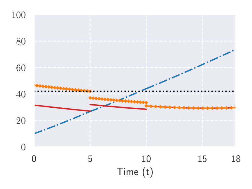
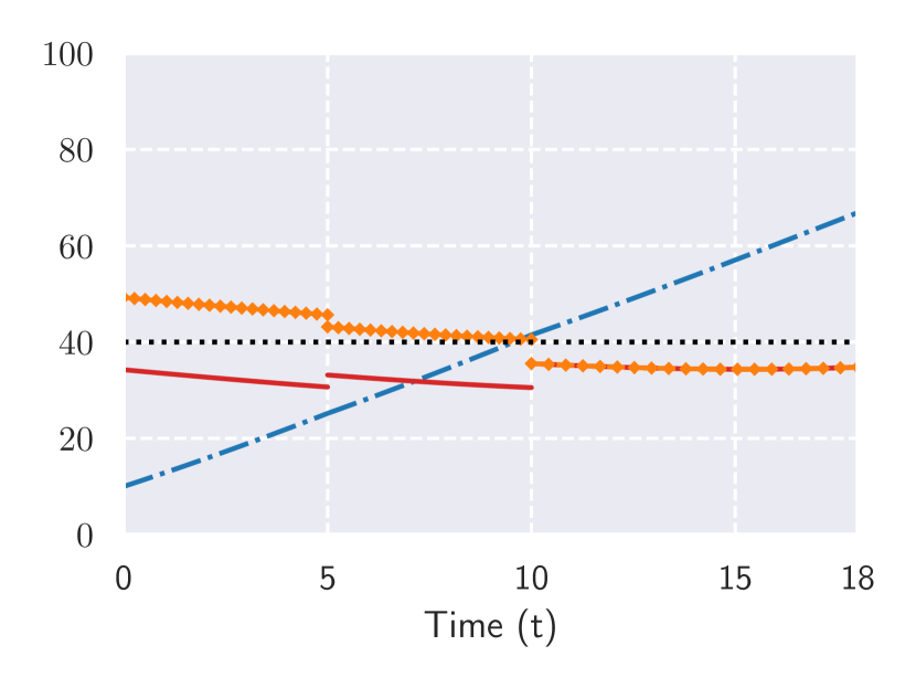
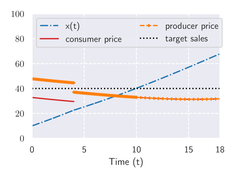
Let the feasible subsidy set be given by $\mathcal{S}=\{0,5,10,{15}\}$ and the subsidy adjustment be made at instants of time $\tau_{1}=0$ and $\tau_{2}=5$. The subsidy program stops at $\tau_{3}=10$, which is different from the firm’s planning horizon, set here to $T=18$. Based on the results, we answer here our research questions 1, 2, and 3.

(a) Without subsidy

(b) With subsidy

(c) Subsidy

Figure 1: Cumulative sales, equilibrium producer and consumer price, and equilibrium subsidy for the benchmark case.

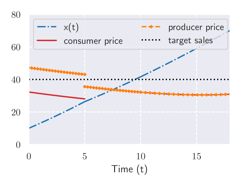
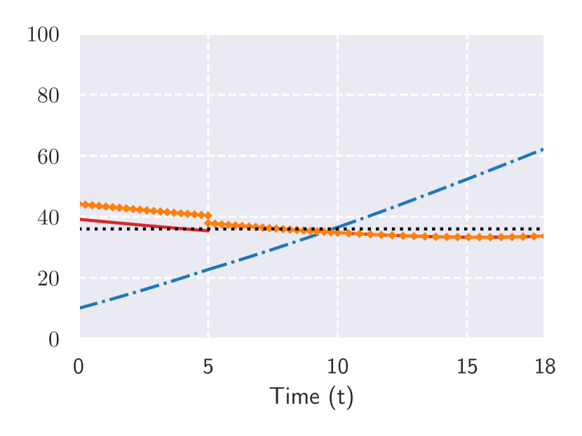
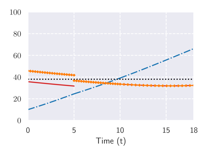
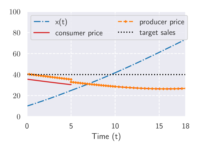
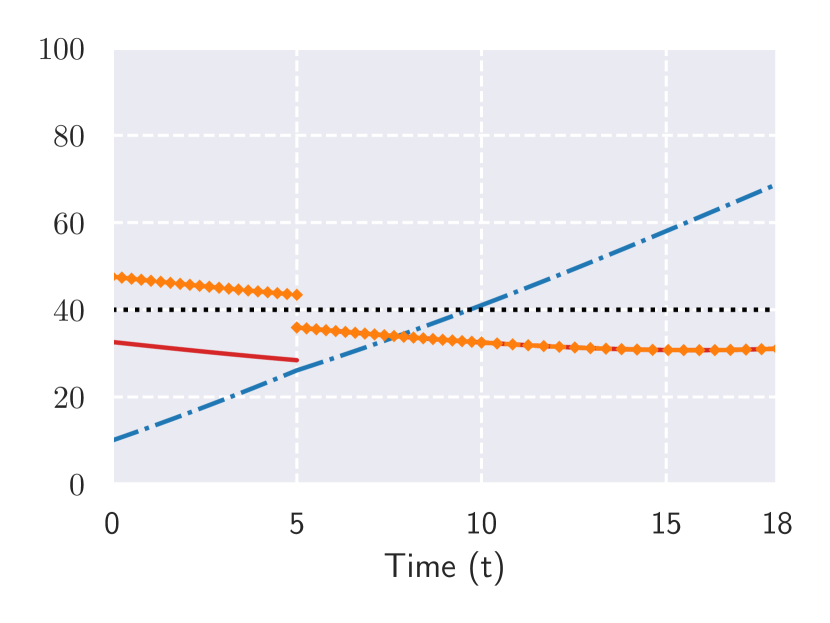
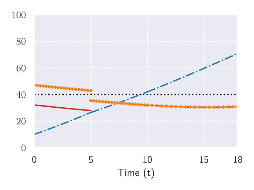
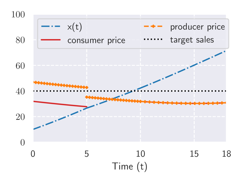
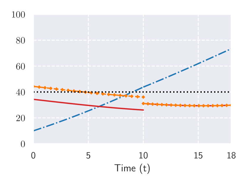
Price and subsidy. Figures 1(a) and 1(b) show that the consumer’s price during the subsidy period is significantly lower than what she would have paid without the subsidy. After the subsidy, the price difference is, however, only slightly lower in the subsidy scenario than in the case without subsidy. In both scenarios, the seller’s price is decreasing over time, which is the consequence of learning-by-doing and word-of-mouth effects.

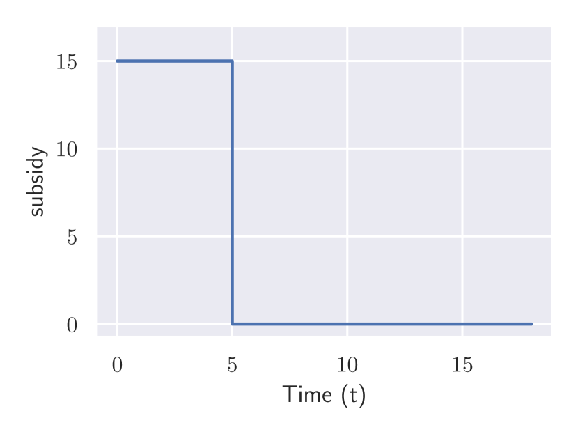
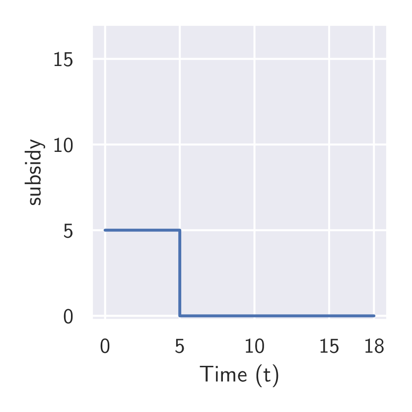
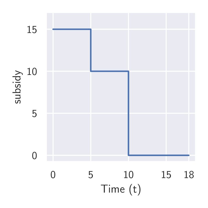
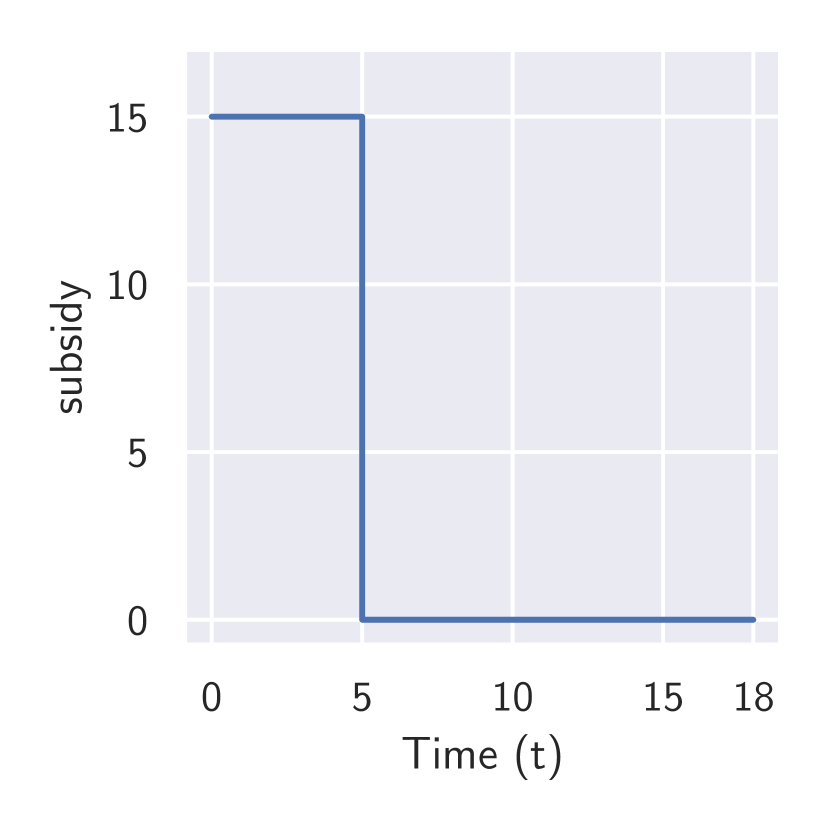
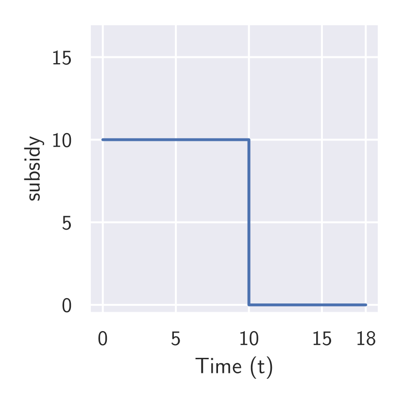
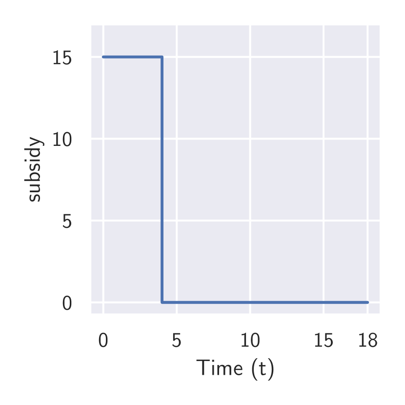
The government sets the subsidy level at $15$ at $\tau_{1}=0$ and at $0$ at time $5$ (see Figure 1(c)). Starting with a high subsidy, slightly more than 25% of the seller’s price, is meant to trigger a snowballing effect in the adoption process. Indeed, high subsidy leads to high demand, which accelerates the reduction in the unit production cost and the positive word-of-mouth effect. In turn, the price goes down and adoption rate up.

Comparing the results in Figures 1(a) and 1(b) shows that the adoption rate is higher when the government offers a subsidy than when it does not, which is expected. Note that the target would not been reached without subsidy.

(a) Target = 36

(b) Target = 38

(c) Target = 42

(d) Target= 44

Figure 2: Cumulative sales, producer and consumer price when target is varied from the benchmark case.

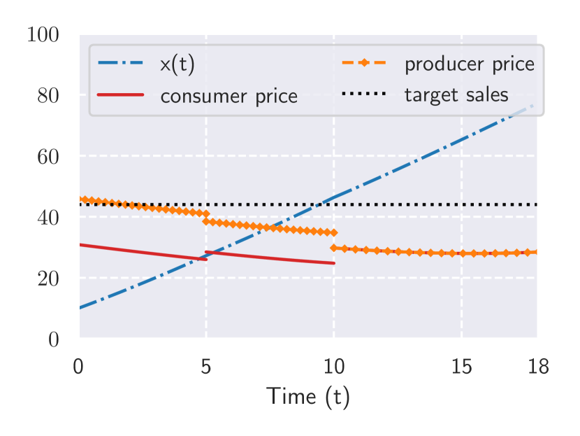
Firm’s strategic behavior.

The subsidy period is given by the time interval $I=\left[0,5\right].$ Denote by $p^{s}\left(t\right)$ the firm’s price when the government offers a subsidy and by $p\left(t\right)$ the price when it does not. Our results show that $p^{s}\left(t\right)>p\left(t\right)$ for all $t\in I$. Then, the answer to our second research question is unambiguous: the firm indeed takes advantage of the implementation of the subsidy program to increase its price during the time interval $I$. One implication of this strategic behavior is that the subsidy program is not achieving its full potential in terms of decreasing the price and raising the adoption rate. The same conclusion was reached in Kaul et al., (2016) and Jiménez et al., (2016) in their evaluation of the car scrappage program.

Cost and benefits.

Whereas the cost of a subsidy program is straightforward to compute, its benefits are more complex to determine. Here, the subsidy program costs taxpayers $1028.43$. The benefits can be assessed in terms of consumer surplus, firm’s profit, and environmental impact.

Consumers are paying a lower price in the subsidy scenarios and buying more. Consequently, consumer surplus is higher with the subsidy. The firm is clearly benefiting from the subsidy. Indeed, its profit is approximately $2560.84$ with subsidy, and $1638.11$ without a subsidy, which is a 56% increase. This big difference comes from two sources. One is the higher sales volume, while the other is the firm’s strategic behavior discussed above. The environmental benefits are more complicated to assess because they depend on a series of assumptions. A first assessment can be done in terms of the number of gasoline cars replaced by EVs, and the saving of gasoline consumption over the useful life of an EV, which depends of the yearly driving distance by a car. From this perspective, independent of how the computations are done, the conclusion would be the same, i.e., subsidizing EVs reduces pollution emissions. Ultimately, however, a comprehensive evaluation should consider all steps involved in the production of the two types of cars from extraction of raw materials to manufacturing and disposing of them when becoming obsolete. Also, one should consider the sources of electricity used to feed the EVs. Clearly, if the source is heavily polluting (coal, fuel), than the benefit (if any) is much lower than when the electricity is produced with renewable technologies.

(a) Target = 36

(b) Target = 38

(c) Target = 42

(d) Target= 44

Figure 3: Equilibrium subsidy when target is varied from the benchmark case.

5.1 Sensitivity analysis

In this section, we vary the values of the main model’s parameters and assess the impact on the results.

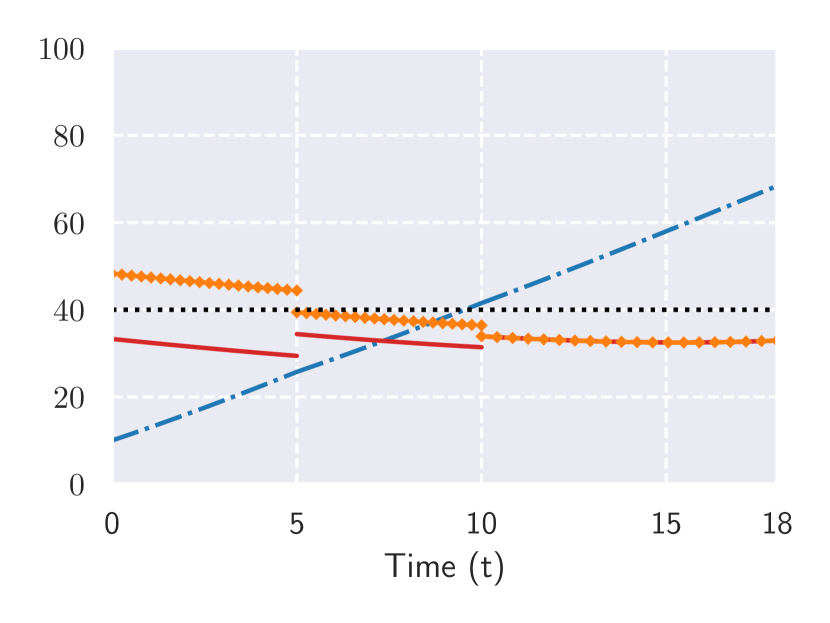
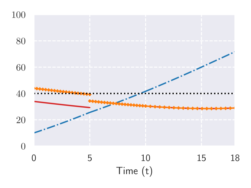
Impact of the target value.

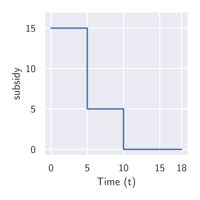
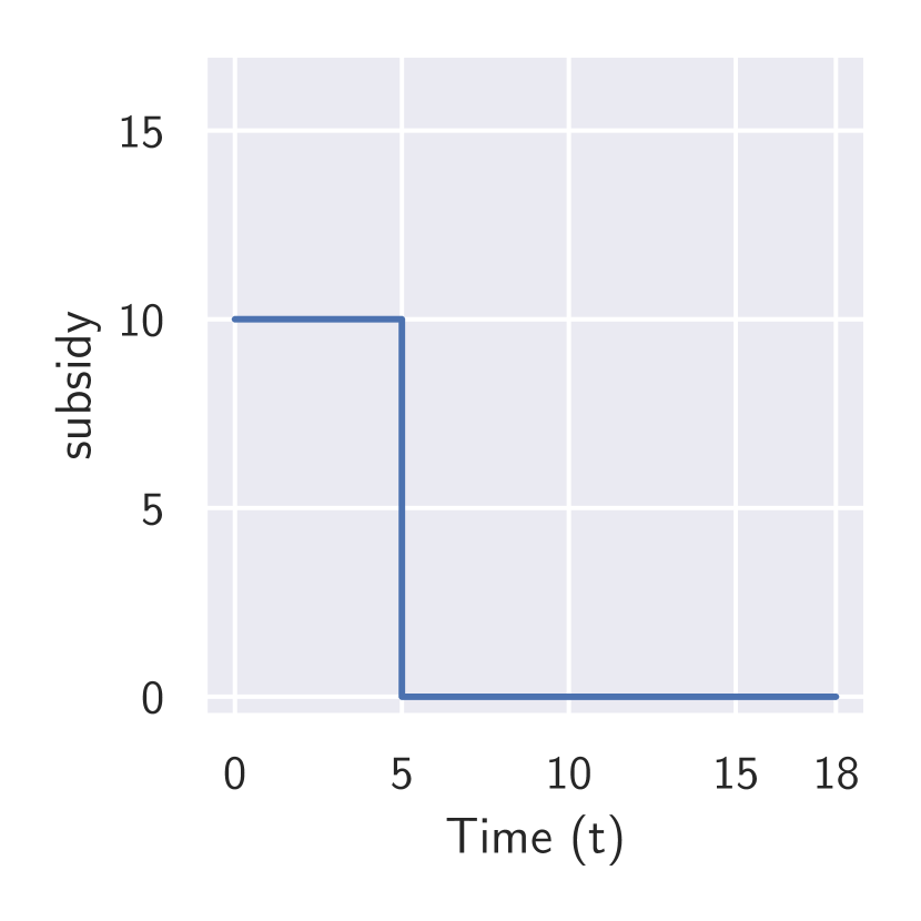
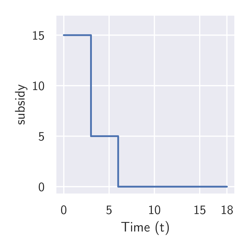
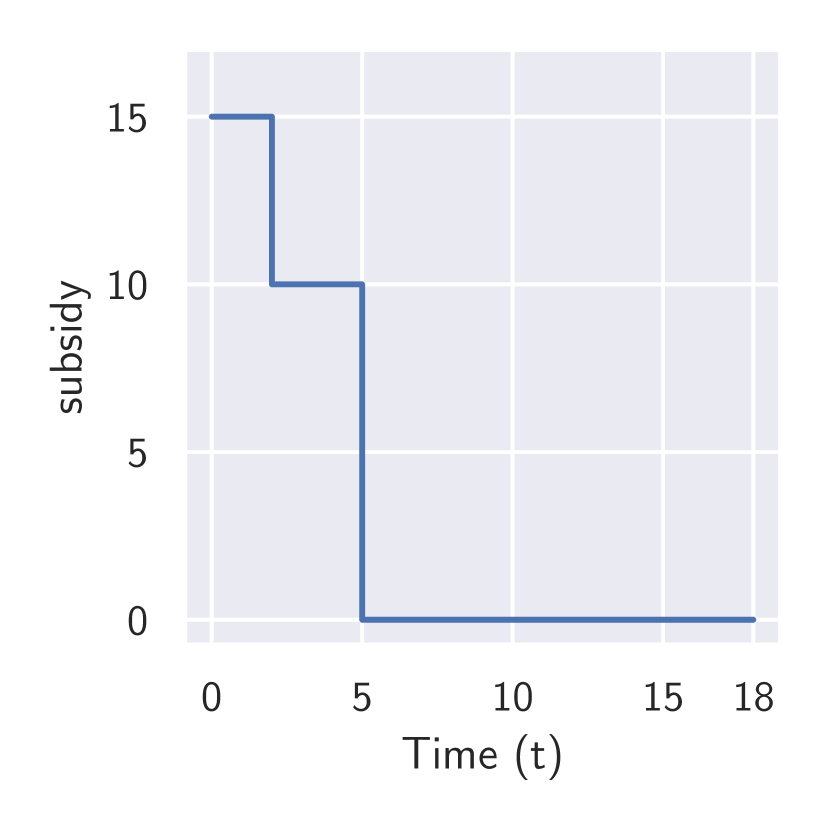
We consider two values to the left of the benchmark target and two to its right. We can see in Figure 2 that if we make the target values lower than the benchmark case, the consumer prices increase significantly during the interval $[5,10]$ as the subsidy offered is reduced from $15$ in the benchmark case, shown in Figure 1(c), to $5$ (Figure 3(a)) and $10$ ( Figure 3(b)). For target levels higher than the benchmark, that is, $x_{s}=$ $42,$ $44$, the terminal consumer price decreases as the subsidy increases in both first and second periods; see Figures 3(c) and 3(d). The cost of the subsidy program for $x_{s}=36,38,42,44$ is $317.08,656.56,1460.75,1914.09$, respectively. Note that the higher the target value, the higher the subsidy and the government’s cost, which is intuitive. What is less intuitive is the order of magnitude in the changes. To illustrate, the cost of the subsidy program increases by $600$%, when the target is up by $22$% (from $36$ to $44$). Finally, the higher the target, the lower the after-subsidy price.

(a) $b_{2}$= 0.72

(b) $b_{2}$= 0.76

(c) $b_{2}$= 0.84

(d) $b_{2}$= 0.88

Figure 4: Equilibrium subsidy plan when $b_{2}$ is varied from the benchmark case.

(a) $b_{2}$= 0.72

(b) $b_{2}$= 0.76

(c) $b_{2}$= 0.84

(d) $b_{2}$= 0.88

Figure 5: Cumulative sales, producer and consumer price when $b_{2}$ is varied from the benchmark case.

Impact of learning speed.

As one can expect, a higher value of the learning speed $b_{2}$ only brings good news. Indeed, we see in Figures 4 and 5 that increasing $b_{2}$ leads to lower price and subsidy. Also, the cost to government is lower; for $b_{2}=0.72,0.76,0.84,0.88$, the subsidy cost is $1783.29,1414.20,674.81,335.56$, respectively. Clearly, the impact of the learning speed is huge. Increasing $b_{2}$ by $22$% (from 0.72 to 0.88) cuts the subsidy bugdet by more than $5$ times ($335.56$ when $b_{2}=0.88$ instead of $1783.29$ when $b_{2}=0.72$).

(a) $\alpha_{2}$= 0.009

(b) $\alpha_{2}$= 0.0095

(c) $\alpha_{2}$= 0.0105

(d) $\alpha_{2}$= 0.011

Figure 6: Equilibrium subsidy when $\alpha_{2}$ is varied from the benchmark case.

Impact of word of mouth.

We study the variation in equilibrium prices and subsidy with the change in $\alpha_{2}$ which measures the word-of-mouth effect. We can see in Figure 6 as $\alpha_{2}$ increases, there is not much variation in the price while the subsidy adjustments do not change, Figure 7. One explanation is that a higher $\alpha_{2}$ means larger market potential, which reduces the incentive to reduce the price to boost demand. The subsidy program cost for $\alpha_{2}=0.009,0.0095,0.0105,0.011$ is given by $1021.77,1025.07,1031.32,1035.32$, respectively. Here, increasing by 22% the value of $\alpha_{2}$ (from $0.009$ to $0.011$), leads to only a 1.3% increase in the budget.

(a) $\alpha_{2}$= 0.009

(b) $\alpha_{2}$= 0.0095

(c) $\alpha_{2}$= 0.0105

(d) $\alpha_{2}$= 0.011

Figure 7: Equilibrium subsidy plan when $\alpha_{2}$ is varied from the benchmark case.

(a) $N$= 1

(b) $N=3$

(c) $N=4$

(d) $N=5$

Figure 8: Equilibrium subsidy when $N$ is varied from the benchmark case.

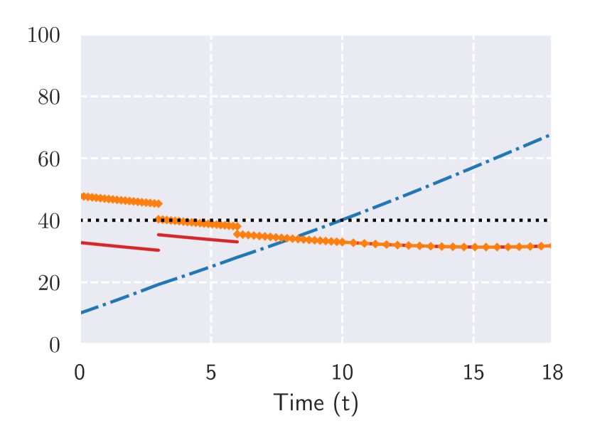
Impact of subsidy adjustments.

Finally, we vary the number of subsidy adjustments in the time interval $[0,10]$. As the number of adjustments increase in Figure 8, the terminal price remains almost the same, while the subsidies are reduced over time (Figure 9). The cost of the government for ${N=1,3,4,5}$ is given by $1473.42,801.03,802.61,798.06$, respectively. There is clearly a decreasing relationship between the number of changes in the subsidy and the cost. A larger number of changes give more degrees of freedom in adjusting the subsidy levels to reach the target. Therefore, the ultimate impact will depend on the target and the fixed cost of each change in the subsidy.

(a) $N=1$

(b) $N=3$

(c) $N=4$

(d) $N=5$

Figure 9: Equilibrium subsidy plan when $N$ is varied from the benchmark case.

6 Conclusions

In this paper, we provide a verification theorem to characterize the feedback-Stackelberg equilibrium in a differential game between a government and a firm. While the firm acts at each instant of time, the government intervenes only at certain discrete time instants to adjust the subsidy level. To the best of our knowledge, it is the fist time that a feedback-Stackelberg equilibrium is determined in a differential game with one player using impulse control. Also, it is the first paper in the diffusion models literature that implements discrete changes to the subsidy, which is more realistic than assuming a continuous modification of its level.

It would be interesting to apply our results to a case study with real-world data on subsidies. Beside this, the two following methodological extensions to our model are of interest:

1. We assumed that the cost function is affine in cumulative production, which may be a good approximation in the short run, but not in the long term. Based on empirical work, Levitt et al., (2013) concludes that “. . . learning is nonlinear: large gains are realized quickly, but the speed of progress slows over time.”  One option is to adopt a hyperbolic cost function that allows to capture this nonlinearity and insure that the cost remains positive for any level of cumulative production; see, e.g., (Janssens and Zaccour,, 2014). However, such modification comes with the additional difficulty in determining the feedback-Stackelberg equilibrium as the game would not be anymore linear-quadratic and one would need to numerically solve the HJB partial differential equation.

2. Another extension is to let the timing of subsidy adjustments be also chosen optimally. This extension would require challenging methodological developments as we do not dispose yet of a theorem characterizing the equilibrium in such setup.

References

- Aïd et al., (2020) Aïd, R., Basei, M., Callegaro, G., Campi, L., and Vargiolu, T. (2020). Nonzero-Sum Stochastic Differential Games with Impulse Controls: A Verification Theorem with Applications. Mathematics of Operations Research, 45(1):205–232.
- Başar and Olsder, (1998) Başar, T. and Olsder, G. J. (1998). Dynamic Noncooperative Game Theory. SIAM, second edition edition.
- Başar and Zaccour, (2018) Başar, T. and Zaccour, G. (2018). Handbook of Dynamic Game Theory. Springer.
- Basei et al., (2022) Basei, M., Cao, H., and Guo, X. (2022). Nonzero-Sum Stochastic Games and Mean-Field Games with Impulse Controls. Mathematics of Operations Research, 47(1):341–366.
- Bass, (1969) Bass, F. M. (1969). A new product growth for model consumer durables. Management science, 15(5):215–227.
- De Cesare and Di Liddo, (2001) De Cesare, L. and Di Liddo, A. (2001). A Stackelberg Game of Innovation Diffusion: Pricing, Advertising, and Subsidy Strategies. International Game Theory Review, 3(4):325–339.
- Dockner and Jørgensen, (1988) Dockner, E. and Jørgensen, S. (1988). Optimal Pricing Strategies for New Products in Dynamic Oligopolies. Marketing Science, 7(4):315–334.
- Dockner et al., (1996) Dockner, E. J., Gaunersdorfer, A., and Jørgensen, S. (1996). Government price subsidies to promote fast diffusion of a new consumer durable. In Jørgensen, S. and Zaccour, G., editors, Dynamic Competitive Analysis in Marketing, pages 101–110. Springer-Verlag, Berlin.
- Eliashberg and Jeuland, (1986) Eliashberg, J. and Jeuland, A. P. (1986). The Impact of Competitive Entry in a Developing Market Upon Dynamic Pricing Strategies. Marketing Science, 5(1):20–36.
- Haurie et al., (2012) Haurie, A., Krawczyk, J. B., and Zaccour, G. (2012). Games and Dynamic Games. World Scientific, Singapore.
- He et al., (2007) He, X., Prasad, A., Sethi, S. P., and Gutierrez, G. J. (2007). A survey of stackelberg differential game models in supply and marketing channels. Journal of Systems Science and Systems Engineering, 16:385–413.
- Islam and Meade, (2000) Islam, T. and Meade, N. (2000). Modelling diffusion and replacement. European Journal of Operational Research, 125(3):551–570.
- Janssens and Zaccour, (2014) Janssens, G. and Zaccour, G. (2014). Strategic price subsidies for new technologies. Automatica, 50(8):1999–2006.
- Jiménez et al., (2016) Jiménez, J. L., Perdiguero, J., and García, C. (2016). Evaluation of subsidies programs to sell green cars: Impact on prices, quantities and efficiency. Transport policy, 47:105–118.
- Jørgensen and Zaccour, (1999) Jørgensen, S. and Zaccour, G. (1999). Price subsidies and guaranteed buys of a new technology. European Journal of Operational Research, 114:338–345.
- Jørgensen and Zaccour, (2004) Jørgensen, S. and Zaccour, G. (2004). Differential Games in Marketing. International Series in Quantitative Marketing. Kluwer Academic Publishers.
- Kalish and Lilien, (1983) Kalish, S. and Lilien, G. L. (1983). Optimal price subsidy for accelerating the diffusion of innovations. Marketing Science, 2:407–420.
- Kaul et al., (2016) Kaul, A., Pfeifer, G., and Witte, S. (2016). The incidence of Cash for Clunkers: Evidence from the 2009 car scrappage scheme in Germany. International Tax and Public Finance, 23(6):1093–1125.
- Levitt et al., (2013) Levitt, S., List, J., and Syverson, C. (2013). Towards an Understanding of Learning by Doing: Evidence from an Automobile Assembly Plant. Journal of Political Economy, 121(4):643–681.
- Li and Sethi, (2017) Li, T. and Sethi, S. P. (2017). A review of dynamic stackelberg game models. Discrete & Continuous Dynamical Systems - B, 22(1):125.
- Lilien, (1984) Lilien, G. L. (1984). Government Support for New Technologies: Theory and Application to Photovoltaics. Applications of Management Science, 2:77–125.
- Mahajan et al., (1993) Mahajan, V., Muller, E., and Bass, F. M. (1993). New-product diffusion models. In Handbooks in Operations Research and Management Science, volume 5, pages 349–408. Elsevier.
- Mahajan et al., (2000) Mahajan, V., Muller, E., and Wind, Y., editors (2000). New-product diffusion models, volume 11. Springer Science & Business Media.
- Peres et al., (2010) Peres, R., Muller, E., and Mahajan, V. (2010). Innovation diffusion and new product growth models: A critical review and research directions. International Journal of Research in Marketing, 27(2):91–106.
- Raman and Chatterjee, (1995) Raman, K. and Chatterjee, R. (1995). Optimal monopolist pricing under demand uncertainty in dynamic markets. Management Science, 41(1):144–162.
- Robinson and Lakhani, (1975) Robinson, B. and Lakhani, C. (1975). Dynamic price models for new-product planning. Management Science, 21(10):1113–1122.
- (27) Sadana, U., Reddy, P. V., Başar, T., and Zaccour, G. (2021a). Sampled-Data Nash Equilibria in Differential Games with Impulse Controls. Journal of Optimization Theory and Applications, 190(3):999–1022.
- (28) Sadana, U., Reddy, P. V., and Zaccour, G. (2021b). Nash equilibria in nonzero-sum differential games with impulse control. European Journal of Operational Research, 295(2):792–805.
- Sadana et al., (2023) Sadana, U., Reddy, P. V., and Zaccour, G. (2023). Feedback Nash Equilibria in Differential Games With Impulse Control. IEEE Transactions on Automatic Control, 68(8):4523–4538.
- Xu et al., (2011) Xu, K., Chiang, W. Y. K., and Liang, L. (2011). Dynamic pricing and channel efficiency in the presence of the cost learning effect. International Transactions in Operational Research, 18(5):579–604.
- Zaccour, (1996) Zaccour, G. (1996). A differential game model for optimal price subsidy of new technologies. Game Theory and Applications, 2:103–114.