Multiple-shot labeling of quantum observables

Abstract

A particular class of quantum observable discrimination tasks, which are equivalent to identifying the outcome label associations of unlabeled observables, was introduced in [Physical Review A 109, 052415 (2024)]. In that work, the tasks were investigated within the “single-shot” regime, where a single implementation of the measurement devices is available. In this work, we explore these tasks for non-binary observables and within the multiple-shot scenario, where we have access to finitely many implementations.

I Introduction

Quantum theory furnishes a prescription to describe its probabilistic and statistical aspects, for all experimental scenarios. For example, when we desire to predict the observed measurement statistics of an experiment, each outcome is completely prescribed by a positive operator, referred to as an “effect”. Even though an effect itself does not describe the physics, it prescribes the probability of occurrence of the associated outcomes. To characterise the measurement statistics, we associate effects, as well as labels, to each mutually exclusive outcome. Moreover, while effects corresponding to a measurement device can be experimentally verified, the choice of labels cannot be tested by using the device alone.

There could be scenarios where the specific mathematical description of the effects associated with a measurement device, implementing an observable, is known in prior but their pairings or associations with outcome labels are lost or unknown. In such scenarios, which arise due to deficiencies pertaining to the users of the device, one would require to identify the lost associations or “labelings” and thereby duly assign a mathematical description to the labels. A particular class of tasks which aim to achieve this was introduced in Ref. [1] and were referred to as “quantum labeling tasks”.

In the aforementioned work, quantum labeling tasks have been identified as a particular case of distinguishability tasks (DT) involving quantum observables; This shall be elaborated in Section II. Quantum distinguishability problems date back to 1969 with the seminal work of Helstrom [2]. In general, we can crudely divide distinguishability tasks into two major classes: quantum state DT’s and higher-order DT’s (those involving quantum channels with memory). Both groups have been extensively studied in the literature [3, 4, 5, 6, 7, 8, 9, 10, 11]. Although quantum state DT’s can be translated into higher-order DT’s, there exist crucial differences between them. One is that, in quantum state distinguishability, if the involved states are non-orthogonal to each other then they can not be perfectly distinguished even with finitely many copies of the states being available. The story is different when it comes to higher-order DT’s; There are cases where channels that produce non-orthogonal states as outputs in a single use can produce orthogonal states if finite uses of the channels can be employed. As a very well-known example, it has been found that any two unitary channels can be perfectly discriminated with some finite uses of the channel [12, 13]. These observations motivates us to investigate labeling tasks within the multiple-shot regime and as such forms a major part of this work.

In what follows, we extend the single-shot labelling of binary observables [1] to non-binary observables having $n$-effects. We find the mathematical expression of minimum-error success probability of labelling $n$-effect observables. Then, we find that no non-binary observable can be labelled unambiguously in a single shot. Furthermore, we find that any amount of assistance through entanglement will not increase our performance. This bolsters our intuition to go beyond single-shot regime to multi-shots labelling. The subsequent investigation reveals that in multi-shot regime, the minimum-error success probability of labeling binary observable expresses itself again in terms of the operator 2-norm distance between the associated effects, thereby extending the result regarding single use case found in [1]. We also find that a $d$-dimensional observable with $n$-effects can be perfectly labelled in $n-1$ shots if there exist at least $n-1$ effects with at least one eigenvalue $1$.

This work is outlined as the following. In section II, we mathematically formulate labeling tasks; Prior to this, we briefly sketch what quantum observables and testers are. In section III, we investigate the case of non-binary observables within the single-shot regime. In section IV, we investigate the task within the multiple-shot regime, for binary as well as non-binary observables. In section V, we introduce schemes for partially identifying labelings and we conclude the work with section VI.

II formulation of the problem

II.1 Quantum observables

An $n$-valued quantum measurement is characterised by its mutually exclusive outcomes $x_{1},\dots,x_{n}$, which are respectively associated with positive operators referred to as “effects”, $M_{1},\dots,M_{n}$; These effects are constrained to sum up to the identity operator, $M_{1}+\dots+M_{n}=\mathbbm{1}$. Even though we can safely identify the measurements as collections of effects for most of the purposes of theoretical study, they are rigorously identified with maps which assign effects to particular outcomes. If we denote $\Omega:=\{x_{1},\dots,x_{n}\}$ as the ordered set of outcome labels and $\mathcal{E}(\mathcal{H})$ as the set of all effects, then a quantum measurement is identified with a normalised positive operator-valued measure (POVM), which we refer to as an “observable” $\mathsf{M}:\Omega\rightarrow\mathcal{E}(\mathcal{H})$ with $\mathsf{M}(x_{k})=M_{k}$. These observables can be modeled as quantum-to-classical measure-and-prepare channels $\mathcal{M}$ (hereafter referred to as “measurement channels”), those which take states $\rho$ of the measured system as input states and outputting states of $n$-dimensional systems as,

$$\mathcal{M}(\rho)=\sum_{x_{k}\in\Omega}\text{Tr}[\rho M_{k}]\outerproduct{x_{k}}{x_{k}}.$$ (1)

When we have the channel representation, as a result of the Choi-Jamiołkowski isomorphism [14, 15] between completely positive maps and positive operators, we can associate the observable $\mathsf{M}$ to the positive operator

$$\Phi_{\mathsf{M}}=(\mathcal{I}\otimes\mathcal{M})[\Psi_{+}]=\sum_{k}M_{k}^{\top}\otimes\outerproduct{x_{k}}{x_{k}},$$ (2)

where $\Psi_{+}=\outerproduct{\psi_{+}}{\psi_{+}}$ is the unnormalised maximally entangled state, with $\ket{\psi_{+}}:=\sum_{j=1}^{d}\ket{jj}\in\mathcal{H}\otimes\mathcal{H}$ and $\{\ket{1},\dots,\ket{d}\}$ being an orthonormal basis of $\mathcal{H}$.

As mentioned earlier, in our work, we study discrimination scenarios of when multiple copies of each of the involved measurement channels are available. These multiple copies, which are, in general, implemented at different points in time, can be considered as a single multiple-time-step quantum process. Such processes are mathematically described by “quantum combs”, which are nothing but Choi-Jamiołkowski operators of these processes satisfying certain causality constraints [16, 17]. Instead of digressing towards discussing general quantum combs and their properties, we restrict ourselves to stating that the comb for an $n$-copy measurement channel $\mathcal{M}$ is given by the Choi-Jamiołkowski operator of the comb as $\Phi_{\mathsf{M}}^{\otimes n}$. Interested readers can visit Ref.[17] for general discussions on combs.

II.2 Quantum testers

The most general experiments or test procedures “measuring” quantum combs are described by single descriptors referred to as “quantum testers” [11, 18, 17]. Within the premise of quantum DT’s, the generality of testers accommodates for the so-called “adaptive” strategies as well as entanglement-assisted strategies. A quantum tester $\mathsf{T}$ measuring a quantum comb with $n$ time steps is characterised by an incomplete network with $n$ open slots (see Fig. 1). As such, we refer such a $\mathsf{T}$ as an $n$-slot tester, oftentimes denoting it as $\mathsf{T}^{(n)}$. The input systems of the tester are labeled by even numbers, starting with 0 and the output systems with odd numbers (See (c) of Figure 1).

Given a set of outcomes $\Delta=\{1,\dots,m\}$ associated with the measurement of an $n$-time step process $\mathcal{C}$, the corresponding $n$-slot tester $\mathsf{T}^{(n)}$ is a collection of positive operators referred to as “process effects” $\{T^{(n)}_{1},\dots,T^{(n)}_{m}\}$, which satisfies the following normalisation conditions,

$$\sum_{x\in\Delta}T^{(n)}_{x} = \Xi^{(n)}\otimes\mathbbm{1}_{2n-1}$$ (3)

$$\text{Tr}_{2k-2}[\Xi^{(n)}] = \Xi^{(k-1)}\otimes\mathbbm{1}_{2k-3}\quad\forall k\in\{2,\dots,n\}$$ (4)

$$\text{Tr}[\Xi^{(1)}] = 1.$$ (5)

These normalisation conditions reflect the causal structure of the tester network. The probability of observing an event $\alpha\in\Delta$ is given by the generalised Born rule $p_{\alpha}=\text{Tr}\left\{\Phi_{\mathcal{C}}T_{\alpha}\right\}$, where $\Phi_{\mathcal{C}}$ is the quantum comb of the process. Moreover, we observe from these conditions that a $1$-slot tester $\mathsf{T}^{(1)}$ has the normalisation condition $\sum_{x}T^{(1)}_{x}=\rho\otimes\mathbbm{1}_{1}$ for some appropriate state $\rho$ on the input system of the channel [18]. We note that such 1-slot testers describe measurements of 1-time step quantum processes. Such 1-slot testers which test measurement channels can be assumed, without loss of generality, to take the form $T_{\alpha}=\sum_{k}H_{k}^{(\alpha)}\otimes\outerproduct{x_{k}}{x_{k}}$ [10], where $\sum_{\alpha}H_{k}^{(\alpha)}=\xi$, for all $k$.

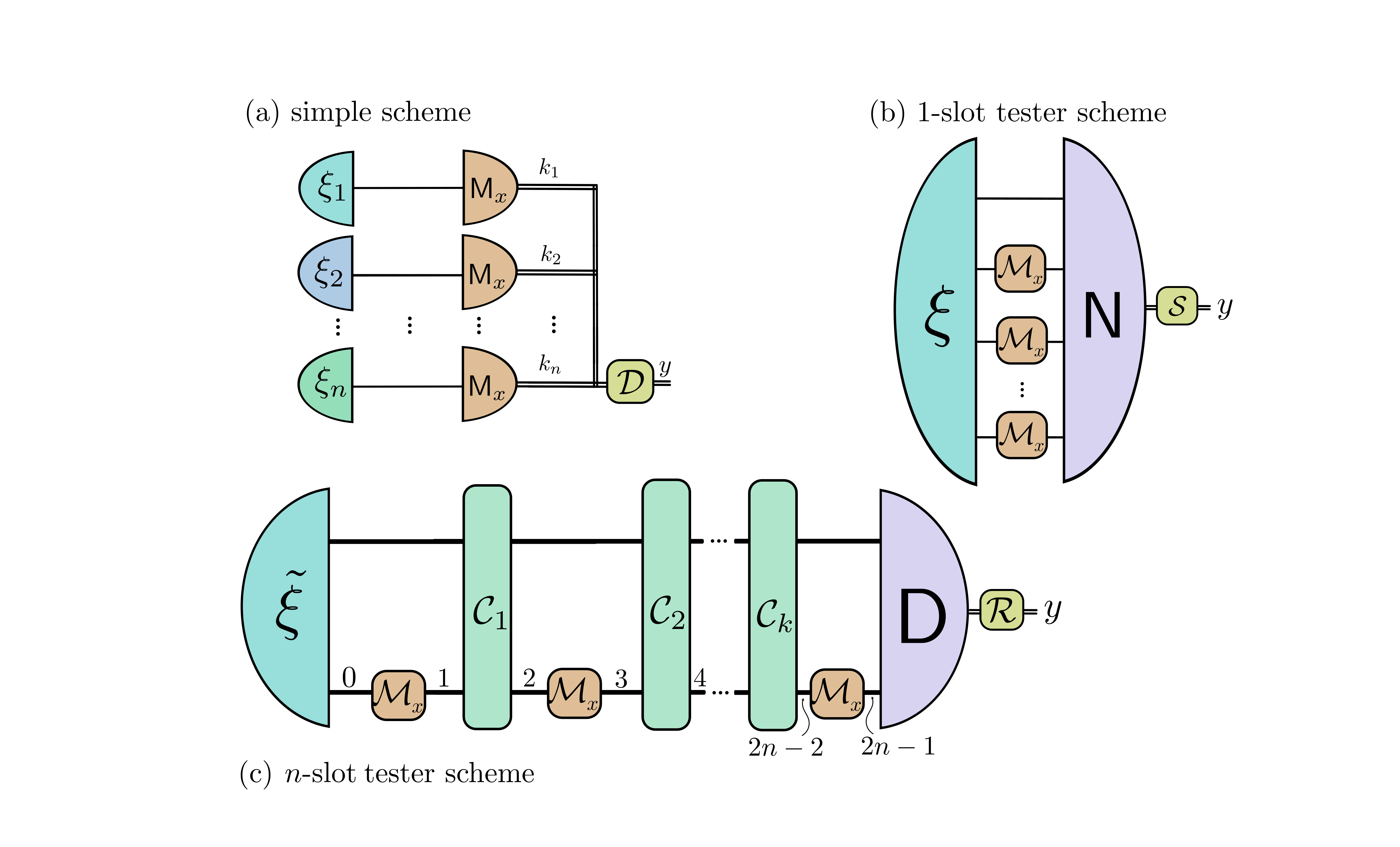
Figure 1: The figure depicts different discrimination tasks using quantum testers: a) a simple scheme where no assistance of entanglement is used, b) one slot tester scheme where assistance of entanglement is used and c) $n$-slot tester scheme where like (b) assistance of entanglement is used, however, a series of intermediate evolutions are also used. Naturally, the last scheme is more powerful in general for any discrimination tasks. Note also that the post-processings are denoted by the operators $\mathcal{D}$, $\mathcal{S}$, and $\mathcal{R}$, those which lead to decisions $y$, essentially identifying $\mathsf{M}_{x}$ as $\mathsf{M}_{y}$.

II.3 Labeling problem

As mentioned in Ref. [1], the aspect of labeling an observable arises when there is a lack of information between the mapping between the outcomes and the associated effects, $x_{k}\mapsto M_{k}$. For the case where all the effects are different, of an observable with $n$ effects, there are $n!$ different possibilities, due to permutations, how the outcomes can be paired with the effects. As such, the aim of the labeling problem is to discriminate among these $n!$ possibilities. Once we fix an order, or equivalently the effect-outcome pairings, $\mathsf{M}_{\pi}$ is the observable obtained by $\pi$-permuting the order.

In our premise of measurement channels, labeling corresponds to discriminating among channels, whose action are given by,

$$\mathcal{C}_{\pi}(X)=\sum_{k}\text{Tr}[XM_{k}]\outerproduct{x_{\pi(k)}}{x_{\pi(k)}}=\mathcal{P}_{\pi}\circ\mathcal{C}_{\text{id}},$$ (6)

where $\mathcal{P}_{\pi}(Y)=P_{\pi}YP_{\pi}$ with $P_{\pi}=\sum_{k}\outerproduct{x_{\pi(k)}}{x_{k}}$ being the permutation operators. Notice that $\mathcal{C}_{\text{id}}$ denote no permutation. We can also observe that this symmetry is translated to the corresponding Choi operators $\Phi_{\pi}$. With $m=n!$, let $T_{1},\dots,T_{m}$ denote the tester describing the labeling experiment of $\mathcal{C}_{1},\dots,\mathcal{C}_{m}$. Then, this experiment is characterised by conditional probabilities $p(\pi|\pi^{\prime})=\text{Tr}[\Phi_{\pi^{\prime}}T_{\pi}]$. The most common performance quantifier of this task is the average error probability

$$p_{e}=1-\frac{1}{n!}\sum_{\pi}p(\pi|\pi),$$ (7)

where $p(\pi|\pi)$ correspond to correct decisions. Minimising $p_{\text{error}}$, we arrive at minimum-error labeling. Admitting an additional inconclusive outcome through $T_{?}$ and strictly requiring to not admit any error, that is $p(\pi|\pi^{\prime})=0$ for all $\pi\neq\pi^{\prime}$, we arrive at unambiguous labeling. Here, when we enjoy error-free conclusions, it is at a cost of decision failures which occurs with a probability

$$p_{f}=\frac{1}{n!}\text{Tr}\left\{\sum_{\pi}\Phi_{\pi}T_{?}\right\}.$$ (8)

Whenever $p_{e}=p_{f}=0$ is achieved, we have “perfect labeling”. Moreover, when we have labeling experiments having access to $n$ copies of the channels, then the conditional probabilities are given by $p(\pi|\pi^{\prime})=\text{Tr}\left\{\Phi_{\pi^{\prime}}^{\otimes n}T_{\pi}\right\}$ and the rest are similar to the above discussion. We can identify the schemes available to us as either “simple”, “1-slot tester”, or “$n$-slot tester” schemes (See Figure 1); We note that these schemes are not strictly exclusive to each other in specific instances. Simple schemes are not assisted by entanglement; We arrive at conclusions by measuring the unlabeled observable, educated probe states and subsequently processing the outcomes. The 1-slot tester schemes are entanglement assisted and the different copies of the unlabeled observables are not correlated to each other by memories. The $n$-slot tester schemes are not only assisted by entanglement but also by quantum memories that the different copies of the measurement channels are correlated to the previous ones, in time.

III Labeling non-binary observables

We refer to observables which have exactly two non-zero effects as “binary” and those which have more than two as “non-binary”. Moreover, in this work, all effects associated with the observables we consider are assumed to be non-zero. In this section, we investigate minimum-error and unambiguous labeling of non-binary observables.

III.1 Minimum-error labeling

Generally, labeling a non-binary observable, composed of non-identical effects, presents itself to be more intricate than that of a binary observable. This complexity arises due to the fact that labeling of such an observable corresponds to a DT concerning $n!$ number of measurement channels. Our approach to non-binary observables begins by examining the minimum-error labeling scenario without entanglement assistance and then we assess whether the more complex entanglement-assisted scenario can improve the performance.

To evaluate the averaged success probability in the simple scheme (see Fig. 1-(a)), we use the following lemma, introduced in Ref. [19], which furnishes the success probability for distinguishing a collection of pairwise commuting states.

Lemma 1 (Theorem 1 in [19]).

Let $\{\rho_{1},\dots,\rho_{n}\}$ be a set of pairwise commuting states appearing with respective a priori probabilities $\{p_{1},\dots,p_{n}\}$. Hence, we have the spectral decomposition $\rho_{j}=\sum_{k}\lambda_{jk}\Pi_{k}$ for all $j$ with $\lambda_{jk}={\rm Tr}[\rho_{j}\Pi_{k}]$. Then, the success probability $p_{\text{s}}$ is given by,

$$p_{\text{s}}=\sum_{k}{\rm Tr}[\Pi_{k}]\max\{{\rm Tr}[p_{1}\rho_{1}\Pi_{k}],\dots,{\rm Tr}[p_{n}\rho_{n}\Pi_{k}]\}.$$ (9)

Notice that the above minimum-error discrimination success probability is always achievable by the measurements composed of the projectors $\{\Pi_{k}\}$.

Deploying this lemma we arrive to the following theorem:

Theorem 1.

A non-binary observable $\mathsf{M}$, composed of $n$ effects $\{M_{1},\dots,M_{n}\}$, can be labeled with the optimal averaged success probability being $p_{\text{s}}^{\text{opt}}=\frac{1}{(n-1)!}\alpha_{\mathsf{M}}$, without the assistance of entanglement, where $\alpha_{\mathsf{M}}:=\max_{\{\rho,M_{j}\}}{\rm Tr}\{\rho M_{j}\}$ and $\rho$ being the state of the system that has been measured.

Proof.

Without entanglement assistance, this DT translates to the simultaneous discrimination of the $n!$ prepared states $\rho_{j}:=\mathcal{P}_{\pi_{j}}(\rho)=\sum_{m}\text{Tr}\left\{\mathsf{M}_{j}(m)\rho\right\}\outerproduct{m}{m}$, when the measured state is $\rho$. We note that this is a collection of mutually commuting states. With respect to the above lemma, we identify $\{\Pi_{m}=\outerproduct{m}{m}\}_{m=1}^{n}$}. For our case in which each observable appears with equal chance, $p_{j}=\frac{1}{n!}$, Eq (9) becomes,

$$p_{\text{s}}= \frac{1}{n!}\{\max\{\text{Tr}\left\{\rho M_{1}\right\},\text{Tr}\left\{\rho M_{2}\right\},\dots,\text{Tr}\left\{\rho M_{n}\right\}\}+$$ (10)

$$\max\{\text{Tr}\left\{\rho M_{2}\right\},\text{Tr}\left\{\rho M_{3}\right\},\dots,\text{Tr}\left\{\rho M_{1}\right\}\}+\dots+$$

$$\max\{\text{Tr}\left\{\rho M_{n}\right\},\text{Tr}\left\{\rho M_{1}\right\},\dots,\text{Tr}\left\{\rho M_{n-1}\right\}\}\}$$

$$= \frac{1}{n!}n\cdot\max\{\text{Tr}\left\{\rho M_{1}\right\},\text{Tr}\left\{\rho M_{2}\right\},\dots,\text{Tr}\left\{\rho M_{n}\right\}\}$$

$$= \frac{1}{(n-1)!}\max_{M_{j}}\{\text{Tr}\left\{\rho M_{j}\right\}\}.$$

Now, optimising over the possible states $\rho$, and denoting $\alpha_{\mathsf{M}}:=\max_{\{\rho,M_{j}\}}\text{Tr}[\rho M_{j}]$, we arrive at the optimal success probability as the following, completing the proof.

$$p_{s}^{\text{opt}}=\frac{1}{(n-1)!}\alpha_{\mathsf{M}}.$$ (11)

∎

The next natural question one can ask is whether the above $p_{s}^{\text{opt}}$ we achieve, without the assistance of entanglement, can be improved through schemes with entanglement-assistance. Consequent addressal of this question results in the following theorem, telling us that entanglement-assistance is of no aid in improvement.

Theorem 2.

For a non-binary observable $\mathsf{M}$, composed of $n$ effects $\{M_{1},\dots,M_{n}\}$, the optimal average success probability obtained by the no-entanglement protocol, $p_{\text{s}}=\frac{1}{(n-1)!}\alpha_{\mathsf{M}}$, is optimal over all protocols. This implies that a more general entanglement-assisted protocol cannot improve it.

Proof.

We prove the theorem for a three-effect observable, $\mathsf{M}=\{M_{1},M_{2},M_{3}\}$. Assuming there are no identical effects, there are six non-identical observables and their corresponding Choi-Jamiołkowski operators $\Phi_{k}$ which we need to discriminate in order to label. As such, the quantum tester testing these observables are given by $\{\mathsf{T}_{c}=\sum_{i}H_{i}^{(c)}\otimes\outerproduct{i}{i}\}$ with $c\in\{1,\dots,6\}$ and $\sum_{c}H_{j}^{(c)}=\rho$ for all $j$. Then, the average probability of success $p_{s}$ is given by $p_{s}=\sum_{j}p_{j}\text{Tr}[\mathsf{T}_{j}\Phi_{j}]$. Plugging in the expressions for $\mathsf{T}_{j}$ and $\Phi_{j}$ and using the notation $H_{x}^{\alpha\beta}=H_{x}^{(\alpha)}+H_{x}^{(\beta)}$, we have,

$$p_{s} = \frac{1}{3!}\text{Tr}\left\{M_{1}H_{1}^{12}+M_{2}H_{1}^{34}+M_{3}H_{1}^{56}\right\}$$

$$+\frac{1}{3!}\text{Tr}\left\{M_{1}H_{2}^{35}+M_{2}H_{2}^{16}+M_{3}H_{2}^{24}\right\}$$

$$+\frac{1}{3!}\text{Tr}\left\{M_{1}H_{3}^{46}+M_{2}H_{3}^{25}+M_{3}H_{3}^{13}\right\}.$$

Consider the term appearing in the first summand as $\Lambda=\text{Tr}\left\{M_{1}H_{1}^{12}+M_{2}H_{1}^{34}+M_{3}H_{1}^{56}\right\}$. Knowing that $H_{1}^{12}+H_{1}^{34}+H_{1}^{56}=\rho,$ without loss of generality, we can assume $H_{1}^{12}=w_{1}\sigma_{1},H_{1}^{34}=w_{2}\sigma_{2},\text{and }H_{1}^{56}=w_{3}\sigma_{3}$, where $w_{i}$’s are probabilities adding up to one and $\sigma_{i}$’s are some density operators. Now we have,

$$\Lambda =\sum_{i=1}^{3}w_{i}\text{Tr}\left\{M_{i}\sigma_{i}\right\}\leq\sum_{i=1}^{3}w_{i}\max_{\sigma_{i}}\text{Tr}\left\{M_{i}\sigma_{i}\right\}$$ (12)

$$\leq\max_{i}[\max_{\sigma_{i}}\text{Tr}\left\{M_{i}\sigma_{i}\right\}]=\max_{\sigma.M_{i}}\text{Tr}\left\{M_{i}\sigma\right\}=\alpha.$$

Thus, we find that the first summand $\frac{1}{3!}\Lambda$ is upper bounded by $\frac{1}{3!}\alpha$. Similar analyses can be carried out for the second and third summand, leading to similar conclusions that both of them are separately upper bounded by $\frac{1}{3!}\alpha$. Thus, we have the following inequality

$$p_{s}\leq\frac{1}{3!}(\alpha+\alpha+\alpha)=\frac{1}{3!}3\alpha=\frac{1}{2!}\alpha.$$ (13)

Comparing this inequality and Eq(11), with $n=3$, we can conclude that the average success probability furnished by Eq(11) is fact the optimal one over all possible protocols, including entanglement-assisted ones. This analysis can be extended to non-binary observables composed of finite $n$ effects, arriving at the conclusion that $p_{s}=\frac{1}{(n-1)!}\alpha_{\mathsf{M}}$ is the optimal average success probability. ∎

The optimal labeling procedure involves preparing the state $\ket{\omega}$ such that the value of $\alpha=\max_{j}\bra{\omega}M_{j}\ket{\omega}$ for $j=1,\cdots,n$ can be obtained. Let’s consider the scenario of a three-effects observable $\{M_{1},M_{2},M_{3}\}$, where $M_{1}$ has the maximum eigenvalue, i.e., $\alpha=\bra{\omega}M_{1}\ket{\omega}$. The optimal protocol can be envisioned as a straightforward scheme: first, feed the corresponding unlabeled observable channel with state $\ket{\omega}$, and then measure the outcomes with a three-dimensional projective measurement.

In an experimental setup, the effects of this projective measurement are observed on the measurement device, which may consist of three colorful bulbs or three detectors representing possible paths of a particle. For example, if the second detector clicks (or the second bulb shines), the corresponding labeling could be either $\{M_{2},M_{1},M_{3}\}$ or $\{M_{3},M_{1},M_{2}\}$. The decision between these two possibilities can be determined by feeding the measurement with a second probe $\ket{\omega^{\prime}}$ that maximizes the value $|\bra{\omega^{\prime}}(M_{2}-M_{3})\ket{\omega^{\prime}}|$.

It is worth mentioning that the maximum value for the probability of success can be obtained when $\alpha_{\mathsf{M}}=1$, and it happens when at least one of the effects has an eigenvalue one or in other words the maximum value is obtainable if there is a $\ket{\varphi}$ such that for an effect $M_{j}$, $M_{j}\ket{\varphi}=\ket{\varphi}$. which means that $M_{i}$ can be perfectly labeled.

The minimum value can be obtained for the most pathological case i.e. a measurement with $M_{i}=\frac{1}{n}\mathbbm{1}$ for all $i$. In this case, $\alpha_{\mathsf{M}}=\frac{1}{n}$ and thus $p_{s}=\frac{1}{n!}$. In the following, we can look at the specific classes of observables.

von Neumann observables. An observable is von Neumann if each of its composing effects is a rank-1 projector. As such, $n=d$ and $\alpha_{\mathsf{M}}=1$ and we notice that the success probability decreases with the dimension of the system as

$$p_{s}=\frac{1}{(d-1)!}.$$ (14)

Trine measurement. A choice of trine measurement, which is an observable with three rank-1 effects, is given by,

$$M_{1}=\frac{2}{3}\ket{0}\bra{0},M_{2}=\frac{2}{3}\ket{v_{+}}\bra{v_{+}},M_{3}=\frac{2}{3}\ket{v_{-}}\bra{v_{-}},$$ (15)

where $\ket{v_{\pm}}=\frac{1}{2}\ket{0}\pm\frac{\sqrt{3}}{2}\ket{1}$. In this case, $\alpha=\frac{2}{3}$ that can be obtainable with each of the states $\ket{0}$, $\ket{v_{+}}$, or $\ket{v_{-}}$. Therefore, the minimum-error success probability for labelling this observable is $p_{s}=\frac{1}{3}$.

III.2 Unambiguous labeling

The labeling procedure is considered unambiguous when the so-called no-error conditions are met, and inconclusive results are permissible. In [1], it was found that in the context of binary observables, unambiguous labeling equates to perfect labeling. However, in the scenario of non-binary observables, achieving perfect labeling has been deemed unattainable in a single-shot. This prompts the question of whether it is feasible to establish unambiguous protocols that enable error-free labeling of effects while acknowledging a nonzero probability of failure in the process.

A non-binary observable $\mathsf{M}$, composed of non-identical effects $\{M_{1},\dots,M_{n}\}$ is unambiguously labelable if there exists a quantum tester $\mathsf{T}$ having $(n!+1)$ process effects, $\{\mathsf{T}_{1},\dots,\mathsf{T}_{n!},\mathsf{T}_{?}\}$ and normalisation $\sum_{j}\mathsf{T}_{j}+\mathsf{T}_{?}=\xi\otimes\mathbbm{1}$, such that the following no-error conditions are met

$$\text{Tr}\left\{\Phi_{x}\mathsf{T}_{j}\right\}_{j\neq x,?} = 0\quad\forall x,j.$$ (16)

Here, $\Phi_{x}$ are the Choi operators for the measurement channels $\mathcal{M}_{x}$ and the process effect $\mathsf{T}_{?}$ is associated with the inconclusive result when no conclusion regarding labeling is made. Our goal is to design a tester such that the failure probability $p_{f}=\Tr{\mathsf{T}_{?}\sum_{j}\Phi_{j}}$ is minimized. A nontrivial solution is possible if the non-error conditions can be simultaneously met, with at least one of the $\mathsf{T}_{j}$’s being a non-zero operator. Investigation of this task results in following theorem, which states that a nontrivial one-shot unambiguous labeling for non-binary measurements is impossible.

Theorem 3.

A non-binary observable $\mathsf{M}$, composed of $n$ effects $\{M_{1},\dots,M_{n}\}$, cannot be unambiguously labeled in a single shot.

Proof.

Let us look at the case with $n=3$ and non-identical effects, then we have six observables with their corresponding Choi operators $\Phi_{j}$. From the no-error conditions, we have $\text{Tr}\left\{\Phi_{1}\mathsf{T}_{2}\right\}=\text{Tr}\left\{\Phi_{1}\mathsf{T}_{3}\right\}=\dots=\text{Tr}\left\{\Phi_{1}\mathsf{T}_{6}\right\}=0$. With $\Phi_{1}=\outerproduct{1}{1}\otimes M_{1}+\outerproduct{2}{2}\otimes M_{2}+\outerproduct{3}{3}\otimes M_{3}$, and $\mathsf{T}_{\alpha}=\sum_{k}H_{k}^{(\alpha)}\otimes\outerproduct{k}{k}$, we end up with the conditions $\text{Tr}\left\{H_{1}^{2}M_{1}\right\}=\dots=\text{Tr}\left\{H_{1}^{6}M_{1}\right\}=0$. Then, similarly from $\Phi_{2}=\outerproduct{1}{1}\otimes M_{1}+\outerproduct{1}{1}\otimes M_{3}+\outerproduct{3}{3}\otimes M_{2}$ and the unambiguous conditions it is constrained to satisfy, we find that $\text{Tr}\left\{H_{1}^{1}M_{1}\right\}=0$. Adding this condition and the previous ones, and using the normalization condition $\sum_{\alpha}H_{k}^{(\alpha)}=\rho$, we have $\text{Tr}\left\{\sum_{c}H_{1}^{(c)}M_{1}\right\}=\text{Tr}\left\{\rho M_{1}\right\}=0$. Using the unambiguous conditions for all possible labeling, we also find that $\text{Tr}\left\{\rho M_{2}\right\}=\text{Tr}\left\{\rho M_{3}\right\}=0$. Consequently, $\text{Tr}[\rho M_{1}]+\text{Tr}[\rho M_{2}]+\text{Tr}[\rho M_{3}]=\text{Tr}[\rho]=0$, which implies that there does not exist a valid state $\rho$ and, consequently, any test procedure that implements this unambiguous task. This analysis can be carried out for any $n$-effect non-binary observable, completing the proof. ∎

IV multiple-shot labeling

In Ref. [1], the authors majorly studied labeling tasks when a single implementation of the associated unlabeled measurement devices are available. In this section, we address the cases when multiple implementations are available.

IV.1 Perfect labeling of binary observables

Perfect labeling of unlabeled observables in multiple-shots corresponds to the scenario where, after a finite number of uses of the associated measurement channels, one can conclusively identify the labelings. In Ref. [1], it has been found that a binary observable can be perfectly labeled, in a single shot, if and only if at least one of the two composing effects is not full-rank. As such, we can ask this question: Given a binary observable $\mathsf{M}$ that is not perfectly labelable in a single shot, i.e., its effects $M_{1}$ and $M_{2}$ are both full rank operators, is it possible to perfectly label it in the multiple-shot regime, when most general protocols are accessible? The answer to this question is investigated in this subsection, and is expressed through the following theorem that follows.

Let $\mathsf{M}$, with effects $M_{1}$ and $M_{2}$, and $\mathsf{N}$, with effects $N_{1}$ and $N_{2}$ be the two observables we require to discriminate for the labeling. As such, $M_{1}=N_{2}$ and $M_{2}=N_{1}$.

Theorem 4.

If a binary observable $\mathsf{M}$ does not admit perfect labeling in a single shot, then it does not admit perfect labeling in any finite number of shots.

Proof.

Let us prove the scenario for two shots of the observable. In the case of labeling with the more general adaptive strategies, perfect labeling of $\mathsf{M}$ translates to the existence of binary 2-slot testers $\mathsf{T}^{(2)}\equiv\{\mathsf{T}^{(2)}_{1},\mathsf{T}^{(2)}_{2}\}$, with normalisation conditions, $\mathsf{T}^{(2)}_{1}+\mathsf{T}^{(2)}_{2}=\Xi^{(2)}\otimes\mathbbm{1}$, $\text{Tr}\{\Xi^{(2)}\}=\xi\otimes\mathbbm{1}$, satisfying the condition,

$$\Phi_{\mathsf{M}}\otimes\Phi_{\mathsf{M}}(\Xi^{(2)}\otimes\mathbbm{1})\Phi_{\mathsf{N}}\otimes\Phi_{\mathsf{N}}=O.$$ (17)

Plugging in the expressions for the Choi-Jamiołkowski operators, we arrive at the equation $\sum_{j,x,y}(M_{j}^{\top}\otimes M_{y}^{\top}\otimes\outerproduct{j}{j})\Xi^{(2)}(N_{x}^{\top}\otimes N_{y}^{\top}\otimes\outerproduct{x}{x})=O$, which should be satisfied for all $j,x,y=1,2$. Now, sandwiching this equation, with $\mathbbm{1}\otimes(M_{y}^{\top})^{-1}\otimes\mathbbm{1}$ from left and with $\mathbbm{1}\otimes(N_{y}^{\top})^{-1}\otimes\mathbbm{1}$ from right, we are left with $\sum_{j,x,y}(M_{j}^{\top}\otimes\mathbbm{1}\otimes\outerproduct{j}{j})\Xi^{(2)}(N_{x}^{\top}\otimes\mathbbm{1}\otimes\outerproduct{x}{x})=O$. Now, tracing out the system $\mathcal{H}_{2}$ from this equation, and deploying the tester normalisation, we end up with,

$$\sum_{j,x}(M_{j}^{\top}\otimes\outerproduct{j}{j})(\text{Tr}_{2}\{\Xi^{(2)}\})(N_{x}^{\top}\otimes\outerproduct{x}{x})=O$$ (18)

$$\sum_{j,x}(M_{j}^{\top}\otimes\outerproduct{j}{j})(\xi\otimes\mathbbm{1})(N_{x}^{\top}\otimes\outerproduct{x}{x})=O$$ (19)

$$\sum_{x}(M_{x}^{\top}\xi N_{x}^{\top})\otimes\outerproduct{x}{x}=O.$$ (20)

From the positivity of the operators $\outerproduct{x}{x}$, the above equations of perfect labelability translate to $M_{x}^{\top}\xi N_{x}^{\top}=O$ for $\forall x$. Using similar arguments from the previous proof, we can conclude that $\xi=O$. Consequently, there does not exist any 2-slot tester, describing adaptive protocols, that can result in perfect labelability. This proof for two shots can be extended to any finite $N$ shots, where you search for an $N$-slot tester and end up with the same conclusion. ∎

IV.2 Minimum-error labeling of binary observables

Since we have seen that binary observables those cannot be labeled in a single shot can neither be labeled in any finite shots, we proceed to characterise the next best thing we can do; That is, to evaluate the optimal averaged error probability for labeling given such observables.

As already established, $\Phi_{\mathsf{M}}$ and $\Phi_{\mathsf{N}}$ are the Choi operators of the two measure-and-prepare channels we want to discriminate in order to label the observable. Then, following the discussion in Sec.II, the corresponding Choi operators for two shots of the observable are written as $\Phi_{\mathsf{M}}^{\otimes 2}$ and $\Phi_{\mathsf{N}}^{\otimes 2}$. Let us denote by $\mathsf{T}_{\mathsf{M}}$ and $\mathsf{T}_{\mathsf{N}}$ the elements of tester associated with the labelings $\{M_{1},M_{2}\}$ and $\{M_{2},M_{1}\}$, respectively, and satisfying the normalisation condition $\mathsf{T}_{\mathsf{M}}+\mathsf{T}_{\mathsf{N}}=\Xi^{(2)}\otimes\mathbbm{1}$. Then the average error probability reads

$$p_{e}=\frac{1}{2}\left\{\text{Tr}\left\{\mathsf{T}_{\mathsf{M}}\Phi^{\otimes 2}_{\mathsf{N}}\right\}+\text{Tr}\left\{\mathsf{T}_{\mathsf{N}}\Phi^{\otimes 2}_{\mathsf{M}}\right\}\right\}$$ (21)

$$\>\>=\frac{1}{2}\left\{\text{Tr}\left\{\mathsf{T}_{\mathsf{M}}(\Phi_{\mathsf{N}}^{\otimes 2}-\Phi_{\mathsf{M}}^{\otimes 2})\right\}+\text{Tr}\left\{(\Xi^{(2)}\otimes\mathbbm{1})(\Phi_{\mathsf{M}}^{\otimes 2})\right\}\right\}.$$

Evaluating the second term in the above equation, one can show that $\text{Tr}\left\{(\Xi^{(2)}\otimes\mathbbm{1})(\Phi_{\mathsf{M}}^{\otimes 2})\right\}=1$. Therefore, rendering the error probability as $p_{\text{error}}=\frac{1}{2}\left\{1+\text{Tr}\left\{\mathsf{T}_{\mathsf{M}}(\Phi_{\mathsf{N}}^{\otimes 2}-\Phi_{\mathsf{M}}^{\otimes 2})\right\}\right\}$. As such, we have to minimise the term $\text{Tr}\left\{\mathsf{T}_{\mathsf{M}}(\Phi_{\mathsf{N}}^{\otimes 2}-\Phi_{\mathsf{M}}^{\otimes 2})\right\}$. Considering the spectral decomposition of the operators $(\mathsf{M}_{i}\otimes\mathsf{M}_{j}-\mathsf{N}_{i}\otimes\mathsf{N}_{j})=\sum_{x}\sigma_{x}^{ij}\outerproduct{\omega_{x}^{ij}}{\omega_{x}^{ij}}$, we have

$$\text{Tr}\left\{\mathsf{T}_{\mathsf{M}}(\Phi_{\mathsf{M}}^{\otimes 2}-\Phi_{\mathsf{N}}^{\otimes 2})\right\}=\sum_{ijx}\sigma_{x}^{ij}\bra{ij\omega_{x}^{ij}}\mathsf{T}_{12}\ket{ij\omega_{x}^{ij}}$$ (22)

$$=\sum_{x}\sigma_{x}^{11}\{\bra{11\omega_{x}^{11}}\mathsf{T}_{12}\ket{11\omega_{x}^{11}}-\bra{22\omega_{x}^{11}}\mathsf{T}_{12}\ket{22\omega_{x}^{11}}\}$$

$$+\sum_{x}\sigma_{x}^{12}\{\bra{12\omega_{x}^{12}}\mathsf{T}_{12}\ket{12\omega_{x}^{12}}-\bra{21\omega_{x}^{12}}\mathsf{T}_{12}\ket{12\omega_{x}^{21}}\}.$$

Here, we have used the fact that $\sigma_{x}^{11}=-\sigma_{x}^{22}$, and $\sigma_{x}^{12}=-\sigma_{x}^{21}$. For the aforementioned minimisation, we need to suppress positive terms and maximise the negative ones. The negativity or positivity of the terms depends solely on the values of $\sigma_{x}^{11}$, and $\sigma_{x}^{12}$ because the operator $\mathsf{T}_{\mathsf{M}}$ is positive. We know there is one positive and one negative term for each nonzero value of $|\sigma_{x}^{11}|$ and $|\sigma_{x}^{12}|$. Set $\mathsf{T}_{12}$ to vanish on all positive terms then we can write the average error probability as

$$p_{e}=\frac{1}{2}\left\{1-\sum_{x}\absolutevalue{\sigma_{x}^{11}}p_{x}+\absolutevalue{\sigma_{x}^{21}}q_{x}\right\}.$$ (23)

where $i=1$ ($k=1,l=2$) if $\sigma_{x}^{11}<0$ ($\sigma_{x}^{12}<0$) and $i=2$ ($k=2,l=1$) if $\sigma_{x}^{11}\geq 0$ ($\sigma_{x}^{12}\geq 0$), and $p_{x}=\innerproduct{\omega_{x}^{11}ii}{\mathsf{T}_{12}|\omega_{x}^{11}ii}$ and $q_{x}=\innerproduct{\omega_{x}^{12}kl}{\mathsf{T}_{12}|\omega_{x}^{12}kl}$ ($k\neq l$), due to normalisation $\mathsf{T}_{12}\leq\Xi^{(2)}\otimes\mathbbm{1}$, are some sub-normalized probability distribution where

$$p_{x}+q_{x} = \innerproduct{\omega_{x}^{11}ii}{\mathsf{T}_{12}|\omega_{x}^{11}ii}+\innerproduct{\omega_{x}^{12}kl}{\mathsf{T}_{12}|\omega_{x}^{12}kl}\leq\innerproduct{\omega_{x}^{11}ii}{\mathbbm{1}\otimes\Xi^{(2)}|\omega_{x}^{11}ii}+\innerproduct{\omega_{x}^{12}kl}{\mathbbm{1}\otimes\Xi^{(2)}|\omega_{x}^{12}kl}$$ (24)

$$= \innerproduct{\omega_{x}^{11}i}{\Xi^{(2)}|\omega_{x}^{11}i}+\innerproduct{\omega_{x}^{12}l}{\Xi^{(2)}|\omega_{x}^{12}l}\leq\sum_{\ket{e_{x}}}\innerproduct{\omega_{x}^{11}i}{\Xi^{(2)}|\omega_{x}^{11}i}+\sum_{\ket{e_{x}}}\innerproduct{\omega_{x}^{12}l}{\Xi^{(2)}|\omega_{x}^{12}l}$$

$$= \innerproduct{e_{x_{1}}\otimes i}{\mathbbm{1}\otimes\rho|e_{x_{1}}\otimes i}+\innerproduct{e_{x_{2}}\otimes l}{\mathbbm{1}\otimes\rho|e_{x_{2}}\otimes l}=\innerproduct{e_{x_{1}}}{\rho|e_{x_{1}}}+\innerproduct{e_{x_{2}}}{\rho|e_{x_{2}}}=1$$

Moreover, it can be seen that $p_{x}+q_{x}>0$ immediately ends up in a contradiction. If we consider the projective measurement ($\lambda_{1}=1$ and $\lambda_{2}=0$), then the error probability gives a negative value. So, $p_{x}+q_{x}$ can not exceed one.
Provided that $p_{x}+q_{x}\leq 1$, the optimal error probability is achieved when we have

$$p_{e}=\frac{1}{2}\left\{1-\max\{\max_{x}\absolutevalue{\sigma_{x}^{11}},\max_{x}\absolutevalue{\sigma_{x}^{12}}\}\right\}$$ (25)

which can be achieved while using $\mathsf{T}_{12}=\outerproduct{\omega_{x}^{\text{max}}kl}{\omega_{x}^{\text{max}}kl}$, where $\outerproduct{\omega_{x}^{\text{max}}kl}{\omega_{x}^{\text{max}}kl}$ is associated with the largest eigenvalues of $\absolutevalue{\sigma_{x}^{11}}$, or $\absolutevalue{\sigma_{x}^{12}}$, respectively.

Because of the normalization $M_{1}+M_{2}=\mathbbm{1}$, it follows that all the operators of the form $M_{i}\otimes M_{j}-M_{j}\otimes M_{i}$ are commutative, therefore, they share the same system of eigenvectors. Consider a qubit measurement with the spectral decomposition of $M_{1}$ as $M_{1}=\sum_{i}\lambda_{i}\outerproduct{e_{i}}{e_{i}}=\lambda_{1}\outerproduct{e_{1}}{e_{1}}+\lambda_{2}\outerproduct{e_{2}}{e_{2}}$ such that $\lambda_{1}\geq\lambda_{2}$. Then, we can write

$$M_{1}\otimes M_{1}-M_{2}\otimes M_{2} = \sum_{i,j}(\lambda_{i}+\lambda_{j}-1)\outerproduct{e_{i}e_{j}}{e_{i}e_{j}},$$

$$M_{1}\otimes M_{2}-M_{2}\otimes M_{1} = \sum_{i,j}(\lambda_{i}-\lambda_{j})\outerproduct{e_{i}e_{j}}{e_{i}e_{j}},$$ (26)

Therefore, $\sigma_{x}^{11}\in\{2\lambda_{1}-1,\lambda_{1}-\lambda_{2}-1,\lambda_{1}-\lambda_{2}-1,2\lambda_{2}-1\}$ and $\sigma_{x}^{12}=\in\{0,\lambda_{1}-\lambda_{2},\lambda_{1}-\lambda_{2},0\}$ are the set of eigenvalues corresponding to the set of eigenvectors $\{\ket{e_{1}}\ket{e_{1}},\ket{e_{1}}\ket{e_{2}},\ket{e_{2}}\ket{e_{1}},\ket{e_{2}}\ket{e_{2}}\}$. The maximum value of $|\sigma_{x}^{12}|$ is simply $\lambda_{1}-\lambda_{2}$. For $|\sigma_{x}^{12}|$ the maximal value is achieved with either with the maximum or minimum values of $\lambda_{i}$. For the case if $\lambda_{1}\geq\lambda_{2}\geq\frac{1}{2}$, the $\max_{x}\sigma_{x}^{11}=(2\lambda_{1}-1)\geq\max_{x}\sigma_{x}^{12}$. The same result is true for $\lambda_{1}\geq\frac{1}{2}\geq\lambda_{2}$ provided that $\lambda_{1}+\lambda_{2}\geq 1$, otherwise $\max_{x}|\sigma_{x}^{11}|=(1-2\lambda_{2})\geq\max_{x}|\sigma_{x}^{12}|$. And finally, if both $\lambda_{1}$ and $\lambda_{2}$ are smaller than $\frac{1}{2}$, again we have $\max_{x}\sigma_{x}^{11}=(1-2\lambda_{2})\geq\max_{x}|\sigma_{x}^{12}|$.

Consequently, $\max_{x}|\sigma_{x}^{12}|$ never suppress $\max_{x}|\sigma_{x}^{11}|$ then as a result the probability of success is

$$p_{e}^{(2)}=\frac{1}{2}\left(1-\max_{x}\absolutevalue{\sigma_{x}^{11}}\right)$$

$$\quad=\frac{1}{2}\left(1-\|M_{1}\otimes M_{1}-M_{2}\otimes M_{2}\|_{2}\right),$$ (27)

where the operator $2$-norm defined as $\|X\|_{2}=\sup_{\varphi\neq 0}\innerproduct{X\varphi}{X\varphi}/\innerproduct{\varphi}{\varphi}=\lambda_{\max}$, where $\lambda_{\max}$ denotes the largest singular value of $X$.
It is important to compare this result with the probability of error in the single-shot case. In [1], the probability of error was found as $p_{\text{e}}=\frac{1}{2}(1-||M_{1}-M_{2}||_{2})$. Using the spectral decomposition of effects $M_{1}=\sum_{i}\lambda_{i}\outerproduct{e_{i}}{e_{i}}$, one can write

$$\|M_{1}-M_{2}\|_{2} = \max\left\{|1-2\lambda_{1}|,|1-2\lambda_{2}|\right\}$$ (28)

$$= \|M_{1}\otimes M_{1}-M_{2}\otimes M_{2}\|_{2},$$

which means that two uses of a binary observable can not increase the probability of success for labeling.

The above analysis can be generalised to finite $n$ shots of the binary observable, which can be cast into in the following theorem.

Theorem 5.

The optimal error probability $p_{e}^{(n)}$ for the minimum-error labeling of a binary observable $\mathsf{M}$, composed of the effects $M_{1}$ and $M_{2}$, with finite $n$ shots of observable is given by,

$$p_{e}^{(n)}=\frac{1}{2}\left(1-\norm{M_{1}^{\otimes n}-M_{2}^{\otimes n}}_{2}\right).$$ (29)

Since the one-shot and two-shots scenarios result in identical optimal error probabilities, we are inclined to investigate whether this is the case for more number of shots as well. A quick analysis of the above equation reveals that a counter-intuitive result showcasing that with number of uses more than two, the error probability increases.

IV.3 Non-binary observables

As mentioned earlier, in Ref. [1], it was established that perfect labeling of binary measurements in a single shot is achievable if and only if at least one of the effects is rank deficient. Here, we extend this investigation to the case of non-binary measurements in a finite $m$ uses of the measurement device or observable. We begin by presenting the following theorem:

Theorem 6.

A $d$-dimensional observable $\mathsf{M}$ with $n\in[2,d]$ effects can be perfectly labeled, using the simple scheme, in $(n-1)$ shots if and only if there exists at least $(n-1)$ effects having at least one eigenvalue 1.

Proof.

Perfect labeling for an effect $M_{i}$ means the existence of a state such that $M_{i}\ket{\varphi_{i}}\neq 0$ and $M_{j}\ket{\varphi_{i}}=0$ for all $j\neq i$ which result in $\sum_{j\neq i}M_{j}\ket{\varphi_{i}}=0$. Using $\sum_{j}M_{j}=\mathbbm{1}$, we have

$$\sum_{j}M_{j} \ket{\varphi_{i}}=\ket{\varphi_{i}}$$

$$\rightarrow M_{i}\ket{\varphi_{i}}+\sum_{j\neq i}M_{j}\ket{\varphi_{i}}=M_{i}\ket{\varphi_{i}}=\ket{\varphi_{i}},$$ (30)

Then for $M_{i}$ to be labeled perfectly, $\ket{\varphi_{i}}$ has to be an eigenvector with eigenvalue $1$. For a non-binary measurement, to be perfectly labeled, we need $n-1$ effects to be labeled. Therefore at least $n-1$ of effects should have at least one eigenvalue $1$ in their support. The converse is straightforward, if an effect has an eigenvector $\ket{\psi_{i}}$ with eigenvalue 1, i.e. then because of the resolution of the identity ($\sum_{i}M_{i}=\mathbbm{1}$), $\ket{\psi_{i}}$ is in the kernel of all other effects ($M_{j\neq i}\ket{\psi_{i}}=0$). Then $\ket{\psi_{i}}$ can be used to perfectly labeled $M_{i}$ and if $n-1$ effects have eigenvalue $1$ in their support then the measurement can be fully labeled. ∎

Moreover, it is worth mentioning that for a non-binary measurement with $n$ effects, if the measurement can not be perfectly labeled with $n-1$ uses it can not be labeled by increasing the number of uses. In other words, $n-1$ is the fixed number for the possibility of perfect labeling.

Corollary 1.

If a non-binary measurement can be perfectly labeled, then each arbitrary binarization of it (each binary measurement of the form $\{M_{i},\sum_{j\neq i}M_{j}\}$) can be perfectly labeled in a single shot.

Proof.

From Theorem 1 in [1], each binary measurement can be perfectly labeled in one shot if and only if at least one of the effects is rank deficient. For a non-binary measurement with $n$ effects, there are $n$ different binarizations. According to Theorem 6, at least $n-1$ effects should have at least one eigenvalue equal to $1$. Thus, in any binarization, at least one of the effects is rank deficient, and consequently, they are perfectly labeled in one shot. ∎

Utilizing Theorem 6, we can characterize the measurements that can be perfectly labeled within a finite number of uses.

Corollary 2.

Any finite-shot perfectly labeled non-binary measurement with $n$ effects and on a $d$ dimensional space ($d\geq n$) can be parametrized as

$$M_{i}=\outerproduct{e_{i}}{e_{i}}+A_{i},\enspace\forall i\in[1,n-1]\enspace\text{and}\enspace M_{n}=A_{n},$$ (31)

where $\{\ket{e_{i}}\}_{i=1}^{n-1}$ is a an orthonormal basis in a $n-1$ dimensional subspace ($\mathcal{H}_{n-1}$) and $A_{i}$’s are semi positive operators such that $\sum_{i=1}^{n}A_{i}=\mathbbm{1}_{\mathcal{H}_{d}/\mathcal{H}_{n-1}}$.

V Partial and Anti-labeling

In this section, we will address the possibility of labeling an $n$-effect observable at least partially whenever it is impossible to label all the effect perfectly. In this context, it is also relevant that if the partial labeling is not possible, can one exclude some effects resulting in the concept of anti-labeling.

V.1 Partial labeling

Let us consider an $n$-outcome non-binary observable $\mathsf{M}$, composed of effects $\{M_{1},\dots,M_{n}\}$. If this observable has at least one rank-deficient effect, we can identify a strict subset of $m$ effects, $X_{\phi}\subset\{M_{1},\dots,M_{n}\}$ such that the operator $M_{\phi}=\sum_{j\in X_{\phi}}M_{j}$ satisfies $M_{\phi}\ket{\phi}=\ket{\phi}$. As a side note, if there does not exist at least one such strict subset $X_{\phi}$, then we can observe that the observable $\mathsf{M}$ is an observable with all of its effects being full-rank. As such the following procedure is not applicable to such observables. Once we have one $X_{\phi}$, we can perform our measurement of the state $\ket{\psi}$ and conclude that the recorded outcome label corresponds to an effect $M\in X_{\phi}$. This task reduces the ambiguity of the recorded label’s possible association to its effect from $M\in\{M_{1},\dots,M_{n}\}$ to $M\in X_{\phi}$. If it happens that there are more than one such non-identical strict subsets, then we can cross-over to using multiple shots of the observable. Let us consider the case with two such subsets, $X_{\phi_{1}}$ and $X_{\phi_{2}}$, with corresponding operators with action $M_{\phi_{1}}\ket{\phi_{1}}=\ket{\phi_{1}}$ and $M_{\phi_{2}}\ket{\phi_{2}}=\ket{\phi_{2}}$. Then, in the first shot, we measure the state $\ket{\phi_{1}}$ and in the second shot measure the state $\ket{\phi_{2}}$. From the recorded outcomes, we can then conclude that the effect corresponding to the first label satisfies $M_{x}\in X_{\phi_{1}}$ and the second satisfies $M_{y}\in X_{\phi_{2}}$. Since, we do not have any restrictions on the disjointedness between these subsets, it can happen that in both of the shots, the same label is recorded. In this case, we can conclude that $M_{x}\in X_{\phi_{1}}\cap X_{\phi_{2}}$. In such scenarios, the two shots reduce the possibilities even further.

There exists a specific scenario of the above task where, more than enabling us to conclude on the inclusions of the effects, we can identify the effects themselves. This is permitted for those observables for which each of the $m(<n)$ effects in the subset $X_{\phi}=\{M_{1},\dots,M_{m}\}$ is identical to each other, i.e., $M_{\phi}=mM_{1}$. Now, a measurement of the state $\ket{\phi}$ necessarily ensures that the recorded outcome is associated with the effect $M_{1}$. This observation also ensures that the largest eigenvalue of the effect $M_{1}$ is equal to $1/m$ [1]. However, measuring the same probe state $\ket{\phi}$ for the second time will not help us label another unlabelled effect. Now, we can look at the prospects of multiple-shots for this case. Suppose our observable has $k$ subsets, $X_{\phi_{1}},X_{\phi_{2}},\dots,X_{\phi_{k}}$, each of them being a collection of identical effects. Now, in $k$ shots of the observable, we can measure the states, $\ket{\phi_{1}},\ket{\phi_{2}},\dots,\ket{\phi_{k}}$, to perfectly identify to which effects the recorded outcome labels correspond to. So, in $k$ shots, we should be able to identify $k$ labels. Moreover, carrying out subsequent rounds of this experiment can eventually identify all of the labels corresponding to the sets $X_{\phi_{j}}$.

In both examples above, we can in general consider a minmum-error version of partial labeling. The scenario will be modified to the following. Let say you partially label the effect $M_{k}$, then the minimum error for such labeling is equal to

$$p_{e}^{(k)}={\rm Tr}[\outerproduct{\psi}{\psi}_{k}\sum_{j\not\in k}M_{j}]={\rm Tr}[\outerproduct{\psi}{\psi}_{k}(\mathbbm{1}-\tilde{M}_{k})]$$ (32)

Therefore, $p_{e}$ is minimum if ${\rm Tr}[\outerproduct{\psi}{\psi}_{k}\tilde{M}_{k}]$ is maximal. This is equivalent to finding a vector for which we achieve a maximal eigenvalue for $\tilde{M}_{k}$ such that $\lambda_{\max}^{(k)}=m\max_{k}\|M_{k}\|_{\text{op}}$ for each set $k$, where $\|\cdot\|_{\text{op}}$ is the operator norm. Then the minimum error for partial labeling for each $k$ is $p_{e}^{(k)}=1-\lambda_{\max}^{(k)}$.

V.2 Anti-labeling

Let us consider a scenario, where one of the effects $M_{x}$ is rank deficient i.e., $M_{x}\ket{\phi}_{x}=0$. Then it is straightforward to conclude that the recorded outcome cannot be label as $M_{x}$ because of vanishing probability. Instead, all such instances can be excluded $\forall x$. We will call such process anti-labeling as discussed in [1]. A single shot analysis has been discussed in details in [1], and has also been pointed out that rank deficiency is necessary for partial anti-labeling.

For binary measurement, the partial (with zero error) as well as anti-labelling is equivalent to perfect labeling. Now consider, non-binary POVM discussed above. Now, if we do not find an instance where any choice does not result in some $\tilde{M}_{k}$ such that $\tilde{M}_{k}\ket{\psi}_{k}=\ket{\psi}_{k}$, then partial labeling is not possible. However, we can find some probe states $\ket{\phi}_{x}$ for some effects $M_{x}$ for which $M_{x}\ket{\phi}_{x}=0$ $\forall x$. Therefore, all such recorded outcome can be anti-labelled to $M_{x}$ in $x$ shots.

A minimum error anti-labeling can be conceived similar to partial labeling by finding effects $M_{x}$ such that the minimum error to exclude any $x$ is equivalent to finding the quantity $p_{e}^{(x)}=1-{\rm Tr}[\outerproduct{\phi}{\phi}_{x}M_{\bar{x}}]=1-{\rm Tr}[\outerproduct{\phi}{\phi}_{x}(\mathbbm{1}-M_{x})]={\rm Tr}[\outerproduct{\phi}{\phi}_{x}M_{x}]=\epsilon^{(x)}$, where $\epsilon^{(x)}\ll 1$. Evidently, finding minimum eigenstate will serve the purpose.

VI conclusion

In this work, we continued investigating the task of labeling unlabeled quantum measurement devices, that was initiated in Ref. [1]. Ref. [1] studied primarily the task within the premise of single-shot; In this work, we extended the investigations to multiple-shot to probe whether access to more number of copies improve performance of labeling and if so by how much. A curious start was to probe whether binary observables, those do not admit single-shot perfect labeling, would admit multiple-shot perfect labeling. We found this to be not in the affirmative. Moreover, we discovered the following counter-intuitive findings: With two shots, the optimal performance of labeling these observables did not improve but with more shots the performance was falling with the number. Then, we proceeded to characterise perfect labelability for non-binary observables and concluded this work by giving schemes to partially identify or exclude some of the labels of an unlabeled measurement device.

As an extension to the single shot labelling, we establish following results which suppliments our main study in multi-shot regime. We studied minimum-error labeling for non-binary observables and eventually showed that the optimal performance cannot be improved with the assistance of entanglement. Moreover, we showed that non-binary observables cannot be unambiguously labeled with a single use of the measurement device.

References

- Sudarsanan Ragini and Ziman [2024] N. Sudarsanan Ragini and M. Ziman, Single-shot labeling of quantum observables, Physical Review A 109, 052415 (2024).
- Helstrom [1969] C. W. Helstrom, Quantum detection and estimation theory, Journal of Statistical Physics 1, 231 (1969).
- Barnett and Croke [2009] S. M. Barnett and S. Croke, Quantum state discrimination, Advances in Optics and Photonics 1, 238 (2009).
- Bae and Kwek [2015] J. Bae and L.-C. Kwek, Quantum state discrimination and its applications, Journal of Physics A: Mathematical and Theoretical 48, 083001 (2015).
- Bae [2013] J. Bae, Structure of minimum-error quantum state discrimination, New Journal of Physics 15, 073037 (2013).
- Ghoreishi et al. [2019] S. A. Ghoreishi, S. J. Akhtarshenas, and M. Sarbishaei, Parametrization of quantum states based on the quantum state discrimination problem, Quantum Information Processing 18, 1 (2019).
- Rouhbakhsh N and Ghoreishi [2023] M. Rouhbakhsh N and S. A. Ghoreishi, Geometric bloch vector solution to minimum-error discriminations of mixed qubit states, Quantum Information Processing 22, 323 (2023).
- Ziman et al. [2009] M. Ziman, T. Heinosaari, and M. Sedlák, Unambiguous comparison of quantum measurements, Physical Review A 80, 052102 (2009).
- Ziman and Sedlák [2010] M. Ziman and M. Sedlák, Single-shot discrimination of quantum unitary processes, Journal of Modern Optics 57, 253 (2010).
- Sedlák and Ziman [2014] M. Sedlák and M. Ziman, Optimal single-shot strategies for discrimination of quantum measurements, Physical Review A 90, 052312 (2014).
- Chiribella et al. [2008] G. Chiribella, G. M. D’Ariano, and P. Perinotti, Memory effects in quantum channel discrimination, Physical review letters 101, 180501 (2008).
- Acin [2001] A. Acin, Statistical distinguishability between unitary operations, Physical review letters 87, 177901 (2001).
- D’Ariano et al. [2001] G. M. D’Ariano, P. L. Presti, and M. G. Paris, Using entanglement improves the precision of quantum measurements, Physical review letters 87, 270404 (2001).
- Choi [1975] M.-D. Choi, Completely positive linear maps on complex matrices, Linear algebra and its applications 10, 285 (1975).
- Jamiołkowski [1972] A. Jamiołkowski, Linear transformations which preserve trace and positive semidefiniteness of operators, Reports on Mathematical Physics 3, 275 (1972).
- chi [2008] Quantum circuit architecture, Physical review letters 101, 060401 (2008).
- Chiribella et al. [2009] G. Chiribella, G. M. D’Ariano, and P. Perinotti, Theoretical framework for quantum networks, Physical Review A—Atomic, Molecular, and Optical Physics 80, 022339 (2009).
- Ziman [2008] M. Ziman, Process positive-operator-valued measure: A mathematical framework for the description of process tomography experiments, Physical Review A 77, 062112 (2008).
- Ghoreishi and Ziman [2021] S. A. Ghoreishi and M. Ziman, Minimum-error discrimination of thermal states, Physical Review A 104, 062402 (2021).