Zeju Li  zeju.li@ndcn.ox.ac.uk
FMRIB Centre, Wellcome Centre for Integrative Neuroimaging, University of Oxford, Oxford, UK Ying-Qiu Zheng ying-qiu.zheng@ndcn.ox.ac.uk
FMRIB Centre, Wellcome Centre for Integrative Neuroimaging, University of Oxford, Oxford, UK Chen Chen chen.chen2@sheffield.ac.uk
Department of Computer Science, University of Sheffield, Sheffield, UK
Department of Engineering Science, University of Oxford, Oxford, UK
Department of Computing, Imperial College London, London, UK
Saad Jbabdi saad.jbabdi@ndcn.ox.ac.uk
FMRIB Centre, Wellcome Centre for Integrative Neuroimaging, University of Oxford, Oxford, UK Corresponding author

Learning Label Refinement and Threshold Adjustment for Imbalanced Semi-Supervised Learning

Zeju Li  zeju.li@ndcn.ox.ac.uk
FMRIB Centre, Wellcome Centre for Integrative Neuroimaging, University of Oxford, Oxford, UK Ying-Qiu Zheng ying-qiu.zheng@ndcn.ox.ac.uk
FMRIB Centre, Wellcome Centre for Integrative Neuroimaging, University of Oxford, Oxford, UK Chen Chen chen.chen2@sheffield.ac.uk
Department of Computer Science, University of Sheffield, Sheffield, UK
Department of Engineering Science, University of Oxford, Oxford, UK
Department of Computing, Imperial College London, London, UK
Saad Jbabdi saad.jbabdi@ndcn.ox.ac.uk
FMRIB Centre, Wellcome Centre for Integrative Neuroimaging, University of Oxford, Oxford, UK Corresponding author

Abstract

Semi-supervised learning (SSL) algorithms struggle to perform well when exposed to imbalanced training data. In this scenario, the generated pseudo-labels can exhibit a bias towards the majority class, and models that employ these pseudo-labels can further amplify this bias. Here we investigate pseudo-labeling strategies for imbalanced SSL including pseudo-label refinement and threshold adjustment, through the lens of statistical analysis. We find that existing SSL algorithms which generate pseudo-labels using heuristic strategies or uncalibrated model confidence are unreliable when imbalanced class distributions bias pseudo-labels. To address this, we introduce SEmi-supervised learning with pseudo-label optimization based on VALidation data (SEVAL) to enhance the quality of pseudo-labelling for imbalanced SSL. We propose to learn refinement and thresholding parameters from a partition of the training dataset in a class-balanced way. SEVAL adapts to specific tasks with improved pseudo-labels accuracy and ensures pseudo-labels correctness on a per-class basis. Our experiments show that SEVAL surpasses state-of-the-art SSL methods, delivering more accurate and effective pseudo-labels in various imbalanced SSL situations. SEVAL, with its simplicity and flexibility, can enhance various SSL techniques effectively. The code is publicly available .

Keywords: Imbalanced Semi-Supervised Learning, Pseudo-Labeling, Long-Tailed Learning

1 Introduction

Semi-supervised learning (SSL) algorithms are trained on datasets that contain both labelled and unlabelled samples Chapelle et al. (2009). SSL improves representation learning and refines decision boundaries without relying on large volumes of labelled data, which are labor-intensive to collect. Many SSL algorithms have been introduced, with one of the most prevalent assumptions being consistency Zhou et al. (2003), which requires the decision boundaries to lie in low density areas. As a means of accomplishing this, pseudo-labels are introduced in the context of SSL Scudder (1965), and this concept has been extended to several variants employing diverse pseudo-label generation strategies Laine and Aila (2016); Berthelot et al. (2019b, a); Sohn et al. (2020); Wang et al. (2022b). In the pseudo-labelling framework, models trained with labelled data periodically classify the unlabelled samples, and samples that are confidently classified are incorporated into the training set.

The performance of pseudo-label based SSL algorithms depends on the quality of the pseudo-labels Chen et al. (2023). In real-world applications, the performance of these SSL algorithms often degrades due to the prevalence of class imbalance in real-world datasets Liu et al. (2019). When trained with imbalanced training data $\mathcal{X}$, the model $f$ will be biased at inference and tends to predict the majority class Cao et al. (2019); Li et al. (2020). Consequently, this heightened sensitivity negatively impacts the pseudo-labels produced by SSL algorithms, leading to an ever increasing bias in models trained with these labels.

Therefore, finding a better way to obtain pseudo-labels for imbalanced SSL algorithms is an important and popular research topic. But it remains an unsolved problem despite many efforts in this area. In this paper, we examine the process of pseudo-label generation from a statistical viewpoint and derive strategies for pseudo-label refinement and threshold adjustment in a class-imbalanced setup. Surprisingly, we find that although existing heuristic solutions can reduce bias to some extent, they can still be suboptimal. They are either not theoretically sound, or are impacted by the choice of metrics that are not properly designed to identify thresholds for high-quality label selection.

Our key insight (detailed in Section 3) is that both pseudo-label refinement and selection rely on test data distribution. Hence, we propose to utilize a small fraction of distinct labelled datasets, as a proxy for unseen test data, to improve the quality of pseudo-labels . Our method is named SEVAL, which is short for SEmi-supervised learning with pseudo-label optimization based on VALidation data. At its core, SEVAL refines the decision boundaries of pseudo-labels using a partition of the training dataset before proceeding with the standard training process. Similar to AutoML Zoph and Le (2016); Ho et al. (2019), SEVAL can adapt to specific tasks by learning from the imbalanced data itself, resulting in a better fit. Moreover, SEVAL learns thresholds that can effectively prioritize the selection of samples from the high-precision class, which we find is critical but typically overlooked by current model confidence-based dynamic threshold solutions Zhang et al. (2021); Guo and Li (2022).

The contributions of this paper are as follow:

• In the context of pseudo-labelling in imbalanced SSL,we derive the theoretically optimal offsets for pseudo-label refinement and propose efficient strategies for thresholding.

• We propose to learn a curriculum of pseudo-label adjustment offsets using a partition of training data. The derived offsets do not rely on a calibrated model and improve accuracy in both pseudo-labeling and inference.

• We propose to learn a curriculum of thresholds to select correctly classified pseudo-labels using a partition of training data with a novel optimization function. Our strategies outperform existing methods by relaxing the trade-off assumption of Precision and Recall.

• We combine the above mentioned two techniques into a unified learning framework, SEVAL, and find that it outperforms state-of-the-art pseudo-label based SSL methods such as DARP, Adsh, FlexMatch and DASO under various imbalanced scenarios.

2 Related Work

2.1 Semi-Supervised learning

Semi-supervised learning has been a longstanding research focus. The majority of approaches have been developed under the assumption of consistency, wherein samples with similar features are expected to exhibit proximity in the label space Chapelle et al. (2009); Zhou et al. (2003). Compared with graph-based methods Iscen et al. (2019); Kamnitsas et al. (2018), perturbation-based methods Xie et al. (2020); Miyato et al. (2018) and generative model-based methods Li et al. (2017); Gong et al. (2023), using pseudo-labels is a more straightforward and empirically stronger solution for deep neural networks Van Engelen and Hoos (2020). It periodically learns from the model itself to encourage entropy minimization Grandvalet and Bengio (2004). This process helps to position decision boundaries in low-density areas, resulting in more consistent labeling.

Deep neural networks are particularly suited for pseudo-label-based approaches due to their strong classification accuracy, enabling them to generate high-quality pseudo-labels Lee et al. (2013); Van Engelen and Hoos (2020). Several methods have been explored to generate pseudo-labels with a high level of accuracy Wang et al. (2022b); Xu et al. (2021). For example, Mean-Teacher Tarvainen and Valpola (2017) calculates pseudo-labels using the output of an exponential moving average model along the training iterations; MixMatch Berthelot et al. (2019b) derives pseudo-labels by averaging the model predictions across various transformed versions of the same sample; FixMatch Sohn et al. (2020) estimates pseudo-labels of a strongly augmented sample with the model confidence on its weakly augmented version. Many of these approaches falter when faced with class imbalance in the training data, a frequent occurrence in real-world datasets.

2.2 Imbalanced Semi-Supervised Learning

Current pseudo-labelling strategies for SSL algorithms face challenges in real-world data generalization due to class imbalance. Using pseudo-labels in the context of class imbalance can lead to an ever increasing bias towards the majority class during training as more and more samples are pseudo-labelled. Three main categories of methods address this challenge in the literature.

2.2.1 Long-tailed learning-based methods

The first group of methods alters the cost function computed using the labeled samples to train a balanced classifier, consequently leading to improved pseudo-labels. Long-tailed learning presents a complex problem in machine learning, wherein models are trained on data with a distribution characterized by a long tail. In such distributions, classes are imbalanced, with the tail classes consistently being underrepresented. The research on long-tailed recognition Chawla et al. (2002); Kang et al. (2019); Menon et al. (2020); Tian et al. (2020), which focuses on building balanced classifiers through adjusted cost functions or model structures in a fully supervised learning setting, often serves as inspiration for works in imbalanced SSL. For example, BiS He et al. (2021) and SimiS Chen et al. (2022) resample the labelled and pseudo-labelled training datasets to build balanced classifier. ABC Lee et al. (2021) and Cossl Fan et al. (2022) decouple the feature learning and classifier learning with a two head model architecture. Similarly, L2AC Wang et al. (2022a) further decouples the feature and classifier learning by building an explicit bias attractor via bi-level optimization. SAW reweights unlabelled samples from different classes based on the learning difficulties Lai et al. (2022b).

2.2.2 Pseudo-label refinement-based methods

The second category of methods modify targets of the produced pseudo-labels to alleviate the class bias caused by an imbalanced classifier. DARP Kim et al. (2020) refines pseudo-labels by aligning their distribution with the target distribution. SaR Lai et al. (2022a) aligns pseudo-labels to true distributions using distribution alignment-based mitigation vector. On the other hand, logit adjustment (LA) has been explored in the context of SSL to address class bias by shifting the logit using the logarithm of the class priors’ ratio, based on the class frequency from the training dataset Wei and Gan (2023).

2.2.3 Threshold adjustment-based methods

The last group of methods aims to resample unlabelled data to achieve a balanced distribution across classes. Adsh Guo and Li (2022) utilizes an adaptive threshold to ensure that similar portions of pseudo-labels are selected for each class. Built upon FixMatch, FlexMatch and FreeMatch Zhang et al. (2021); Wang et al. (2022c) choose confidently classified samples based on the model’s learning progress, which results in the selection of more samples if the model is not learning well. InPL Yu et al. (2023) proposes to rely on an energy score instead of maximum class probability to select confident samples. InstanT Li et al. (2024) derives instance-wise thresholds based on the sample features. UPS Rizve et al. (2021) utilizes both the confidence and uncertainty of a network prediction to select accurate subsets of pseudo-labels.

Some hybrid methods simultaneously adjust the cost functions and refine the pseudo-labels. For instance, in addition to a bootstrap sampling strategy, CReST+ Wei et al. (2021) utilizes distribution alignment to adjust the class bias of pseudo-labels. DASO Oh et al. (2022) improves pseudo-labels with semantic pseudo-labels and regularizes the feature encoder by aligning balanced semantic prototypes. ACR Wei and Gan (2023) is a holistic approach that builds upon the successes of ABC, FixMatch and MixMatch, and utilizes LA to refine pseudo-labels Menon et al. (2020), yielding impressive results.

In contrast to the above, our proposed method, SEVAL, seamlessly integrates into SSL pipelines without necessitating alterations to the learning strategies, data sampling process, or additional pseudo-label calculations. In addition, unlike many imbalanced SSL algorithms such as DARP and CreST+, SEVAL does not make strong assumptions on the label distribution of unlabelled data. Thus it can be applied to scenarios where the distributions of labelled and unlabelled data are distinct without any modifications.

3 Limitations of Current Methods

In this section, we begin by summarizing the framework of current pseudo-label based semi-supervised learning (SSL). Next, we break down the design of current imbalanced SSL into two key components: pseudo-label refinement and threshold adjustment. We then offer insights into these components through theoretical analysis, highlighting previously overlooked aspects.

3.1 Preliminaries

We consider the problem of $C$-class imbalanced semi-supervised classification. Let $X$ be the input space and $Y=\{1,2,\ldots,C\}$ be the label space. We are given a set of $N$ labelled samples $\mathcal{X}=\{(\bm{x}_{i},y_{i})\}^{N}_{i=1}$ and a set of $M$ unlabelled samples $\mathcal{U}=\{(\bm{u}_{i})\}^{M}_{i=1}$ in order to learn an optimal function or model $f$ that maps the input feature space to the label space $f:X\rightarrow\mathbb{R}_{+}^{C}$. $f$ can be viewed as an estimate of the conditional probability distribution $P(Y|X)$. In deep learning, $f$ can be implemented as a network followed by a softmax function $\sigma$ in order to produce the probability score $p_{c}$ for each class $c$: $p_{c}=\sigma(\bm{z})_{c}=\frac{\mathrm{e}^{z_{c}}}{\sum_{j=1}^{C}\mathrm{e}^{z_{j}}}$ where $\bm{z}$ is the raw output (in $C$-dim) produced by the network. The predicted class is assigned to the one with the highest probability.

Typically, the parameters in $f$ can be optimized by minimizing an empirical risk computed from the labelled dataset $R_{\mathcal{H},\mathcal{X}}(f)=\frac{1}{N}\sum_{i=1}^{N}\mathcal{H}(y_{i},\bm{p}^{\mathcal{X}}_{i})$, where $\bm{p}^{\mathcal{X}}_{i}$ is the model predicted probabilities on the labelled data point and $\mathcal{H}$ can be implemented as the most commonly used cross-entropy loss. To further utilize unlabelled data, a common approach is to apply pseudo-labeling to unlabelled data where the estimated label is generated from the network’s predicted probability vector $\bm{q}\in\mathbb{R}^{C}$  Lee et al. (2013). As there is no ground truth, we use the current model to produce a pseudo-label probability vector $\bm{q}_{i}\in\mathbb{R}^{C}$ for an unlabelled sample $\bm{u}_{i}$ and the pseudo-label $\hat{y}_{i}$ is determined as $\operatorname*{arg\,max}_{j}(q_{ij})$. In this way, we obtain $\hat{\mathcal{U}}=\{(\bm{u}_{i},\hat{y}_{i})\}^{M}_{i=1}$, where each $(\bm{u}_{i},\hat{y}_{i})\in(X\times Y)$. As the predicted label quality can be very poor especially at the early stage and for some challenging data, it is common to apply a threshold to identify reliable labels for model optimization. We describe the case of hard pseudo-labels for simplicity, but the method generalizes to the case of soft pseudo-labels. The risk function on the unlabelled data can be defined as:

$$\hat{R}_{\mathcal{H},\hat{\mathcal{U}}}(f)=\frac{1}{M}\sum_{i=1}^{M}\mathbbm{1}(\max_{j}({q}_{ij})\geq\tau)\mathcal{H}(\hat{y}_{i},\bm{p}^{\mathcal{U}}_{i}),$$ (1)

where $\mathbbm{1}$ is the indicator function and $\tau$ is a predefined threshold that filters out pseudo-labels with low confidence, and $\bm{p}^{\mathcal{U}}_{i}$ is the predicted probability for the unlabelled data.

In a class imbalanced setting, we have a challenge: the distribution of samples across the $C$ classes is highly uneven with varying numbers of samples per class $\mathbf{n}_{C}:{n_{1},...,n_{c}}$. Some classes have many samples (majority classes), while others have very few (minority classes). The class imbalance ratio is defined as $\gamma=\frac{max(\mathbf{n}_{C})}{min(\mathbf{n}_{C})}$, and in an unbalanced setting can e.g., exceed 10. In such case, the pseudo-labels on the unlabelled data can be biased to the majority class, which further amplifies the class imbalance problem. During testing, the model often predicts the majority class instead of the true class.

In this paper, to alleviate the issue of class imbalance-induced bias, we propose a method to refine the probability vector used for pseudo-labelling $\bm{q}_{i}$ . We also propose to adjust the threshold to operate on a class-specific basis, i.e. we use a vector $\bm{\tau}\in\mathbb{R}^{C}$ of threshold values to achieve accuracy fairness. The model can then dynamically select the appropriate thresholds based on its prediction. In the following section, we will bypass the computation of pseudo-label probability $\bm{q}_{i}$ and concentrate on our contributions.

3.2 Pseudo-Label Refinement

	DA Berthelot et al. (2019a)	LA Menon et al. (2020)	DASO Oh et al. (2022)	SEVAL (c.f. Section 4.1)
Estimation of optimal classifier $f_{\mathcal{U}}(X)$	$\displaystyle\frac{f(X)P_{\mathcal{U}}(Y)}{\hat{P}_{\mathcal{U}}(Y)}$	$\displaystyle\frac{f(X)P_{\mathcal{T}}(Y)}{P_{\mathcal{X}}(Y)}$	Blending similarity   based pseudo-label	$\displaystyle\frac{f(X)P_{\mathcal{T}}(Y)}{\bm{\pi}^{*}}$
Note	$\hat{P}_{\mathcal{U}}(Y)$ is the model prediction of $P_{\mathcal{U}}(Y)$. The refined pseudo-label is not optimal on $P_{\mathcal{T}}(X,Y)$.	Inaccurate as $f$ is suboptimal and uncalibrated.	Relying on the effectiveness of blending strategies.	Optimizing the decision boundary on $\mathcal{U}$ using $\mathcal{V}$ as a proxy without assuming a specific $f$.

Table 1: Theoretical comparisons of SEVAL and other pseudo-label refinement methods including distribution alignment (DA) Berthelot et al. (2019a); Wei et al. (2021); Lai et al. (2022a); Kim et al. (2020), logit adjustment (LA) Wei and Gan (2023); Menon et al. (2020) and DASO Oh et al. (2022). $\mathcal{X}$: Labelled training data; $\mathcal{U}$: Unlabelled training data; $\mathcal{T}$: Test data; $\mathcal{V}$: An independent labelled data.

For an unlabelled sample $\bm{u}_{i}$, we determine its pseudo-label probability $\bm{q}_{i}$ based on its corresponding pseudo-label logit $\hat{\bm{z}}_{i}^{\mathcal{U}}$. In the process of pseudo-label refinement, we aim to adjust the decision boundaries for $\hat{\bm{z}}_{i}^{\mathcal{U}}$ with offset $\bm{\pi}\in\mathbb{R}^{C}$ to reduce class biases. Many methods in the literature have been discussed to utilize different $\bm{\pi}$ from different perspectives, such as distribution alignment. However, we find that none of them are suitable for imbalanced SSL. Here, we aim to shed new light on this problem by analyzing optimal threshold adjustment strategies from a statistical perspective Saerens et al. (2002). We assume that the test distribution $\mathcal{T}$ shares identical class conditionals with the training dataset $\mathcal{X}$ (i.e., $P_{\mathcal{X}}(X|Y)=P_{\mathcal{T}}(X|Y)$) and deviates solely in terms of class priors ($P_{\mathcal{X}}(Y)\neq P_{\mathcal{T}}(Y)$), we can assert:

Proposition 1

Given that a classifier $f^{*}(X)$ is optimized on $P_{\mathcal{X}}(X,Y)$,

$$f_{\mathcal{T}}(X)\propto\frac{f^{*}(X)P_{\mathcal{T}}(Y)}{P_{\mathcal{X}}(Y)},$$ (2)

is the optimal Bayes classifier on $P_{\mathcal{T}}(X,Y)$, where $P_{\mathcal{X}}(X|Y)=P_{\mathcal{T}}(X|Y)$ and $P_{\mathcal{X}}(Y)\neq P_{\mathcal{T}}(Y)$.

Corollary 2

The classifier $f_{\mathcal{U}}(X)=f_{\mathcal{T}}(X)$ should be also optimal on the resampled unlabelled data $\displaystyle\frac{P_{\mathcal{U}}(X,Y)P_{\mathcal{T}}(Y)}{P_{\mathcal{U}}(Y)}$, where $P_{\mathcal{T}}(X|Y)=P_{\mathcal{U}}(X|Y)$ and $P_{\mathcal{T}}(Y)\neq P_{\mathcal{U}}(Y)$.

This proposition provides insight into the formulation of pseudo-label offsets: it depends on the distribution of test data, $P_{\mathcal{T}}$, instead of the distribution of unlabelled data, $P_{\mathcal{U}}$. From this analytical viewpoint, we present a summarized Table 1 of current pseudo-label refinement solutions. DA Berthelot et al. (2019a); Wei et al. (2021); Kim et al. (2020) is a commonly employed technique to make balanced prediction for different classes which align the predicted class priors to true class priors of $\mathcal{U}$, making the model being fair Bridle et al. (1991). It only reduces the calibration errors but cannot be optimally fair because it does not take $P_{\mathcal{T}}$ into account. LA modifies the network prediction from $\operatorname*{arg\,max}_{c}(\hat{z}_{ic}^{\mathcal{U}})$ to $\operatorname*{arg\,max}_{c}(\hat{z}_{ic}^{\mathcal{U}}-\lambda\log{\pi_{c}})$, where $\lambda$ is a hyper-parameter and $\bm{\pi}$ is determined as the empirical class frequency Menon et al. (2020); Zhou and Liu (2005); Lazarow et al. (2023). It shares similar design with Eq. 1, however, recall that theorem 1 provides a justification for employing logit thresholding when optimal probabilities $f^{*}(X)$ are accessible. Although neural networks strive to mimic these probabilities, it is not realistic for LA as the classifier is not optimal during training and neural networks are often uncalibrated and over confident Guo et al. (2017). The importance of model calibration for SSL is also highlighted in Loh et al. (2022). The accurate estimation of classifier bias requires the calculation of a conditional confusion matrix, which always requires holdout data Lipton et al. (2018). However, tackling label distribution shifts is rarely discussed in the context of SSL.

3.3 Threshold Adjustment

Here, we look into the impact of pseudo-label quality on the SSL. For simplicity, we consider a model $f$ is trained with $\hat{\mathcal{U}}$ for binary classification using supervised learning loss $\mathcal{L}$. $(\bm{u},\hat{y})$ is an arbitrary sample drawn from $\hat{\mathcal{U}}$. In this section we refer $\mathcal{U}=\{(\bm{u}_{i},y_{i})\}^{M}_{i=1}$ to the oracle distribution which contains the inaccessible real label $y$ for $\bm{u}$. $\rho$ is the noise rate such that $1-\rho=P_{\hat{\mathcal{U}}}(y=\hat{y})$ and $\rho<0.5$. The expected risk is $R_{\mathcal{L},\mathcal{U}}(f):=\mathbb{E}_{(\bm{u},y)\sim\mathcal{U}}[\mathcal{L}(f(\bm{u}),y)]$.

The theorem presented below indicates that, with the number of samples in set $\mathcal{U}$ is fixed as $M$, better model performance is achieved through training with a dataset exhibiting a lower noise rate $\rho$.

Theorem 3

Given $\hat{f}$ is the model after optimizing with $\hat{\mathcal{U}}$. Let $\mathcal{L}$ be $L$-Lipschitz in all the predictions, for any $\delta>0$, with probability at least $1-\delta$,

$$R_{\mathcal{L},\mathcal{U}}(\hat{f})\leq\min_{f\in\mathcal{F}}R_{\mathcal{L},\mathcal{U}}(f)+4L_{p}\mathfrak{R}(\mathcal{F})+2\sqrt{\frac{\log(1/\delta)}{2M}},$$ (3)

where the Rademacher complexity $\mathfrak{R}(\mathcal{F})$ is defined by $\mathfrak{R}(\mathcal{F}):=\mathbb{E}_{\bm{x}_{i},\epsilon_{i}}\left[\sup_{f\in\mathcal{F}}\frac{1}{M}\sum_{i=1}^{M}\epsilon_{i}f(\bm{u}_{i})\right]$ for function class $\mathcal{F}$ and $\epsilon_{1},\ldots,\epsilon_{M}$ are i.i.d. Rademacher variables. $L_{p}\leq\frac{2L}{1-2\rho}$ is the Lipschitz constant.

We provide proofs in Appendix Section A.

The insight of Theorem 3 is simple: given that the label size is fixed at $M$, we should reduce the noise rate $\rho$ for a better model. To achieve this, we want to increase the accuracy of the pseudo-label, of which the marginal distribution over $\hat{y}$ can be calculated as:

$$P_{\hat{\mathcal{U}}}(y=\hat{y})=\sum_{j=1}^{C}\underbrace{P_{\hat{\mathcal{U}}}(y=j|\hat{y}=j)}_{\textbf{Precision}}\underbrace{P_{\hat{\mathcal{U}}}(\hat{y}=j)}_{\emph{Accessible}}.$$ (4)

This indicates that, if we can have an approximation of Precision, we can feasibly tune the pseudo-label accuracy by controlling the sampling strategies based on class-specific thresholds $\bm{\tau}$. However, it is not possible with

$$P_{\hat{\mathcal{U}}}(y=\hat{y})=\sum_{j=1}^{C}\underbrace{P_{\hat{\mathcal{U}}}(\hat{y}=j|y=j)}_{\textbf{Recall}}\underbrace{P_{\hat{\mathcal{U}}}(y=j)}_{\emph{Inaccessible}},$$ (5)

because in practice we do not have the information of ground truth label for $\bm{u}_{i}$. Formally, we claim that:

Lemma 4

A better thresholds $\bm{\tau}$ for choosing effective pseudo-labels should be derived from class-wise Precision, instead of class-wise Recall.

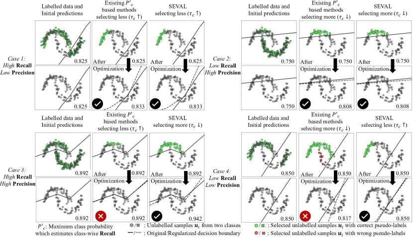
Figure 1: Two-moons toy experiments illustrating the relationship between threshold choice and model performance for class . Accuracy appears in the bottom right. Current maximum class probability-based dynamic thresholding methods such as FlexMatch Zhang et al. (2021), emphasizing Recall, may not be reliable for Case 3 and Case 4. In comparison, SEVAL derived thresholds, reflecting Precision, fit all cases well.

However, existing dynamic threshold approaches Zhang et al. (2021); Wang et al. (2022c); Guo and Li (2022) derive the threshold for class $c$ based on estimated recall. Specifically, they all rely on the maximum class probability of class $c$, i.e. $P^{\prime}_{c}=\frac{1}{K_{c}}\sum_{i=1}^{K}\mathbbm{1}_{ic}\max_{j}{p}_{ij}^{\mathcal{U}}$, where $\mathbbm{1}_{ic}=\mathbbm{1}(\operatorname*{arg\,max}_{j}({p}^{\mathcal{V}}_{ij})=c)$ is 1 if the predicted most probable class is c and 0 otherwise and $K_{c}=\sum_{i=1}^{K}\mathbbm{1}_{ic}$ is the number of samples predicted as $c$. Maximum class probability can be used to estimate accuracy Guo et al. (2017) (which is equivalent to Recall when assessed on a per-class basis since negative samples are not considered) of test samples Garg et al. (2022); Li et al. (2022). Existing dynamic techniques such as FlexMatch tend to prioritize selections from classes linked to lower maximum class probability. Consequently, these approaches lead to a higher sampling frequency from classes exhibiting lower Recall.

We argue that their strategies are built upon the assumption that Recall and Precision is always a trade-off as a result of moving decision boundaries, e.g. low Recall leads to high Precision. However, they would fall short if this does not hold. For example, we should choose as much as possible if the class is well-classified, e.g. high Recall and high Precision. However, following their strategy, they will choose few from them. We illustrate this in Fig. 1 with the two-moons example. While Case 1 and Case 2 are the most common scenarios, current maximum class probability-based approaches struggle to estimate thresholds effectively in other cases. We substantiate this assertion in the experimental section, where we find that Case 3 frequently arises for the minority class in imbalanced SSL and is currently not adequately addressed, as shown in Section 5.6 and Appendix Section D.

4 SEVAL

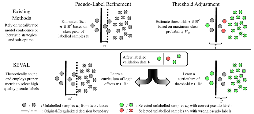
Figure 2: Overview of SEVAL optimization process which consists of two learning strategies aiming at mitigating bias in pseudo-labels within imbalanced SSL scenarios: 1) Pseudo-label refinement and 2) Threshold Adjustment. The curriculum for parameter learning is determined through the evaluation of holdout data performance, ensuring greater accuracy while preventing overfitting.

Fig. 2 shows an overview of SEVAL. The comparative advantage of SEVAL over extant methodologies is summarized in Table 1 and illustrated in Fig. 1. Importantly, we propose to optimize these parameters using a separate labelled holdout dataset. Independent of the training dataset $\mathcal{X}$ and $\mathcal{U}$, we assume we have access to a holdout dataset $\mathcal{V}=\{(\bm{x}_{i},y_{i})\}^{K}_{i=1}$, which contains $k_{c}$ samples for class $c$. We make no assumptions regarding $k_{c}$; that is, $\mathcal{V}$ can either be balanced or imbalanced .

4.1 Learning Pseudo-Label Refinement

We want to further harness the potential of pseudo-label refinement by optimizing $\bm{\pi}$ from the data itself. Assuming the holdout data distribution has the same class conditional likelihood as others and $P_{\mathcal{T}}(Y)$ is uniform, SEVAL can directly estimate the optimal decision boundary as required in Proposition 1. Specifically, the optimal offsets $\bm{\pi}$, are optimized using the labelled holdout data $\mathcal{V}$ with:

$$\begin{multlined}\bm{\pi}^{*}=\operatorname*{arg\,min}_{\bm{\pi}}\frac{1}{K}\sum_{i=1}^{K}\mathcal{H}(y_{i},\bm{p}^{\mathcal{V}}_{i})=\operatorname*{arg\,min}_{\bm{\pi}}\frac{1}{K}\sum_{i=1}^{K}\mathcal{H}(y_{i},\sigma(\bm{z}^{\mathcal{V}}_{i}-\log\bm{\pi})).\end{multlined}\bm{\pi}^{*}=\operatorname*{arg\,min}_{\bm{\pi}}\frac{1}{K}\sum_{i=1}^{K}\mathcal{H}(y_{i},\bm{p}^{\mathcal{V}}_{i})=\operatorname*{arg\,min}_{\bm{\pi}}\frac{1}{K}\sum_{i=1}^{K}\mathcal{H}(y_{i},\sigma(\bm{z}^{\mathcal{V}}_{i}-\log\bm{\pi})).$$ (6)

Subsequently, we can compute the refined pseudo-label logit as $\hat{\bm{z}}_{i}^{\mathcal{U}}-\log\bm{\pi}^{*}$, which are expected to become more accurate on a class-wise basis. Of note, we utilize the final learned $\bm{\pi}^{*}$ to refine the test results and expect it to perform better than LA.

4.2 Learning Threshold Adjustment

We find Precision cannot be solely determined by the network as it also relies on non-maximum probability, as we show in Section 5.6. Thus, here we propose a novel strategy to learn the optimal thresholds based on an external holdout dataset $\mathcal{V}$. We optimize the thresholds in a manner that ensures the selected samples from different classes achieve the same accuracy level of $t$. This is achieved by:

$$\tau_{c}^{*}=\begin{cases}\operatorname*{arg\,min}_{\tau_{c}}\big{|}\mathcal{A}(\tau_{c})-t\big{|}&\text{if}\quad t<\alpha_{c}\\ \quad\quad\quad\quad 0&\text{otherwise}\\ \end{cases},$$ (7)

where $\mathcal{A}(\tau_{c})$ calculates the accuracy of samples where the maximum probability exceeds $\tau_{c}$ :

$$\mathcal{A}(\tau_{c})=\frac{1}{s_{c}}\sum_{i=1}^{K}\mathbbm{1}_{ic}\mathbbm{1}(y_{i}=c)\mathbbm{1}(\max_{j}({p}_{ij}^{\mathcal{V}})>\tau_{c}),$$ (8)

where $s_{c}=\sum_{i=1}^{K}\mathbbm{1}_{ic}\mathbbm{1}(\max_{j}({p}_{ij}^{\mathcal{V}})>\tau_{c})$ is the number of samples predicted as class $c$ with confidence larger than $\tau_{c}$, where $\alpha_{c}=\frac{1}{K_{c}}\sum_{i=1}^{K}\mathbbm{1}_{ic}\mathbbm{1}(y_{i}=c)$ is the average accuracy of all the samples predicted as class $c$.

Notably, the optimized thresholds are inversely related to Precision and possess practical utility in handling classes with varying accuracy. Therefore, we believe this cost function is better suited for fair threshold optimization across diverse class difficulties. In practical scenarios, we often face difficulties in directly determining the threshold through Eq. 7 due to the imbalances in holdout data and constraints arising from a limited sample size. To address these issues, we employ normalized cost functions and group-based learning, detailed further in Appendix Section C.

After obtaining the optimal refinement parameters, for pseudo-label $\hat{y}_{i}=\operatorname*{arg\,max}_{j}(q_{ij})$ and predicted class $y_{i}^{\prime}=\operatorname*{arg\,max}_{j}(p^{\mathcal{U}}_{ij})$, we can calculate the unlabelled loss $\hat{R}_{\mathcal{H},\hat{\mathcal{U}}}(f)=\frac{1}{M}\sum_{i=1}^{M}\mathbbm{1}(\max_{j}({q}_{ij})\geq\tau_{y_{i}^{\prime}})\mathcal{H}(\hat{y}_{i},\bm{p}^{\mathcal{U}}_{i})$ to update our classification model parameters. The estimation process of $\pi$ and $\tau$ is summarized in Algorithm 1.

Algorithm 1 SEVAL parameter estimation process, $\bm{\pi}^{*}$, $\bm{\tau}^{*}$ $\leftarrow$ ESTIM $\left(\mathcal{V},\{\bm{z}_{i}^{\mathcal{V}}\}^{K}_{i=1}\right)$

0:  

1:  $\mathcal{V}=\{(\bm{x}_{i},y_{i})\}^{K}_{i=1}$: validation data, $\{\bm{z}_{i}^{\mathcal{V}}\}^{K}_{i=1}$: network prediction of $\mathcal{V}$.

2:  $C$: Number of classes, $t$: Requested per class accuracy of the pseudo-label, $\bm{k}$: Number of sample per class for $\mathcal{V}$.

3:  $\bm{\pi}^{*}=\operatorname*{arg\,min}_{\bm{\pi}}\frac{1}{K}\sum_{i=1}^{K}\mathcal{H}(y_{i},\sigma(\bm{z}^{\mathcal{V}}_{i}-\log\bm{\pi}))$  $\triangleright$ In practice, the parameter estimation process is achieved by bound-constrained solvers.

4:  $\bm{\omega}^{\mathcal{V}}=1/\bm{k}$    $\triangleright$ The minority class is assigned higher weights to prioritize class-specific accuracy.

5:  for c in C do

6:     Calculate class-wise accuracy $\alpha_{c}=\frac{1}{K_{c}}\sum_{i=1}^{K}\omega_{y_{i}}^{\mathcal{V}}\mathbbm{1}_{ic}\mathbbm{1}(y_{i}=c)$   $\triangleright$ For each class $c$, $\mathbbm{1}_{ic}=\mathbbm{1}(\operatorname*{arg\,max}_{j}({p}^{\mathcal{V}}_{ij})=c)$ and $K_{c}=\sum_{i=1}^{K}\omega_{y_{i}}^{\mathcal{V}}\mathbbm{1}_{ic}$

7:     if $\alpha_{c}>t$ then

8:        $\tau_{c}^{*}=\operatorname*{arg\,min}_{\tau_{c}}\big{|}\frac{1}{s_{c}}\sum_{i=1}^{K}\omega_{y_{i}}^{\mathcal{V}}\mathbbm{1}_{ic}\mathbbm{1}(y_{i}=c)\mathbbm{1}(\max_{j}({p}_{ij}^{\mathcal{V}})>\tau_{c})-t\big{|}$    $\triangleright$ $s_{c}=\sum_{i=1}^{K}\omega_{y_{i}}^{\mathcal{V}}\mathbbm{1}_{ic}\mathbbm{1}(\max_{j}({p}_{ij}^{\mathcal{V}})>\tau_{c})$ is the relative number of samples predicted as class c with confidence larger than $\tau_{c}$

9:     else

10:        $\tau_{c}^{*}=0$    $\triangleright$ The quality of the pseudo-labels is satisfactory, and we make use of all of them.

11:     end if

12:  end for

4.3 Curriculum Learning

To bypass more data collection efforts, we learn the curriculum of $\bm{\pi}$ and $\bm{\tau}$ based on a partition of labelled training dataset $\mathcal{X}$ thus we do not require additional samples. Specifically, before standard SSL process, we partition $\mathcal{X}$ into two subset $\mathcal{X}^{\prime}$ and $\mathcal{V}^{\prime}$ which contain the same number of samples to learn the curriculum.

In order to ensure curriculum stability, we update the parameters with exponential moving average. Specifically, when we learn a curriculum of length $L$, after several iterations, we optimize $\bm{\pi}$ and $\bm{\tau}$ sequentially based on current model status. We then calculate the curriculum for step $l$ as $\bm{\pi}^{(l)}=\eta_{\pi}\bm{\pi}^{(l-1)}+(1-\eta_{\pi})\bm{\pi}^{(l)*}$ and $\bm{\tau}^{(l)}=\eta_{\tau}\bm{\tau}^{(l-1)}+(1-\eta_{\tau})\bm{\tau}^{(l)*}$. We use this to refine pseudo-label before the next SEVAL parameter update. We summarize the training process of SEVAL in Algorithm 2.

Algorithm 2 Imbalanced semi-supervised learning with SEVAL.

0:  

1:  $\mathcal{X}=\{(\bm{x}_{i},y_{i})\}^{N}_{i=1}$: labelled training data, $\mathcal{U}=\{\bm{u}_{i}\}^{M}_{i=1}$: unlabelled training data, $f(\cdot)$: network for classification.

2:  $T$: Total training iterations, $C$: Number of classes, $L$: length of the curriculum, $\eta_{\pi}$, $\eta_{\tau}$: Momentum decay ratio of offsets and thresholds.

3:  Initialize the SEVAL parameters as $l=1$, $\pi$^(l) = $\underbrace{\begin{bmatrix}1,1,\ldots,1\end{bmatrix}}_{C}$ and $\tau$^(l) = $\underbrace{\begin{bmatrix}0.95,0.95,\ldots,0.95\end{bmatrix}}_{C}$.  $\triangleright$ Estimate a curriculum of the SEVAL parameters based on a partition of the training dataset.

4:  Randomly partition $\mathcal{X}$ into two subsets, $\mathcal{X}^{\prime}=\{(\bm{x}_{i},y_{i})\}^{K}_{i=1}$ and $\mathcal{V}^{\prime}=\{(\bm{x}_{i},y_{i})\}^{K}_{i=1}$, each containing an equal number of data points.

5:  for iter in $[1,\ldots,T]$ do

6:     Calculate the pseudo-label logit for unlabelled data $\mathcal{U}$ and obtain $\{\hat{\bm{z}}_{i}^{\mathcal{U}}\}^{M}_{i=1}$.   $\triangleright$ Note: FixMatch achieves this by utilizing two augmented versions of the unlabelled data.

7:     Calculate the pseudo-label probability $\bm{q}_{i}=\sigma(\hat{\bm{z}}_{i}^{\mathcal{U}}-\log\bm{\pi}^{(l)})$.

8:     For pseudo-label $\hat{y}_{i}=\operatorname*{arg\,max}_{j}q_{ij}$ and predicted class $y_{i}^{\prime}=\operatorname*{arg\,max}_{j}p^{\mathcal{U}}_{ij}$, calculate the unlabelled loss $\hat{R}_{\mathcal{H},\hat{\mathcal{U}}}(f)=\frac{1}{M}\sum_{i=1}^{M}\mathbbm{1}(\max_{j}({q}_{ij})\geq\tau^{(l)}_{y_{i}^{\prime}})\mathcal{H}(\hat{y}_{i},\bm{p}^{\mathcal{U}}_{i})$.

9:     Update the network $f$ with labelled loss $\hat{R}_{\mathcal{H},\mathcal{X}}(f)$ calculated using $\mathcal{X}^{\prime}$ and $\hat{R}_{\mathcal{H},\hat{\mathcal{U}}}(f)$ via SGD optimizer.

10:     if $\textbf{iter}\textbf{\%}(T/L)=0$ then

11:        $l=\textbf{iter}L/T$

12:        Calculate the prediction on $\mathcal{V}^{\prime}$ using exponential moving average model and obtain $\{\bm{z}_{i}^{\mathcal{V}}\}^{K}_{i=1}$.

13:        $\bm{\pi}^{(l)*},\bm{\tau}^{(l)*}=\text{ESTIM}(\mathcal{V}^{\prime},\{\bm{z}_{i}^{\mathcal{V}}\}^{K}_{i=1}$)     $\triangleright$ SEVAL parameter estimation process.

14:        $\bm{\pi}^{(l)}=\eta_{\pi}\bm{\pi}^{(l-1)}+(1-\eta_{\pi})\bm{\pi}^{(l)*}$, $\bm{\tau}^{(l)}=\eta_{\tau}\bm{\tau}^{(l-1)}+(1-\eta_{\tau})\bm{\tau}^{(l)*}$

15:     end if

16:  end for $\triangleright$ Standard SSL process.

17:  for iter in $[1,\ldots,T]$ do

18:     $l=\lceil\textbf{iter}L/T\rceil$

19:     Calculate the pseudo-label logit for unlabelled data $\mathcal{U}$ and obtain $\{\hat{\bm{z}}_{i}^{\mathcal{U}}\}^{M}_{i=1}$.

20:     Calculate the pseudo-label probability $\bm{q}_{i}=\sigma(\hat{\bm{z}}_{i}^{\mathcal{U}}-\log\bm{\pi}^{(l)})$.

21:     Calculate the unlabelled loss $\hat{R}_{\mathcal{H},\hat{\mathcal{U}}}(f)=\frac{1}{M}\sum_{i=1}^{M}\mathbbm{1}(\max_{j}({q}_{ij})\geq\tau^{(l)}_{y_{i}^{\prime}})\mathcal{H}(\hat{y}_{i},\bm{p}^{\mathcal{U}}_{i})$.

22:     Update the network $f$ with labelled loss $\hat{R}_{\mathcal{H},\mathcal{X}}(f)$ calculated using $\mathcal{X}$ and $\hat{R}_{\mathcal{H},\hat{\mathcal{U}}}(f)$ via SGD optimizer.

23:  end for $\triangleright$ Post-hoc processing with final learned parameters.

24:  Given a test sample $\bm{x}_{i}$, the logit is adjusted from $\bm{z}_{i}$ to $\bm{z}_{i}-\log\bm{\pi^{(L)*}}$.

5 Experiments

We conducted experiments on several imbalanced SSL benchmarks including CIFAR-10-LT, CIFAR-100-LT Krizhevsky et al. (2009) and STL-10-LT Coates et al. (2011) under the same codebase, following Oh et al. (2022). Specifically, we choose wide ResNet-28-2 Zagoruyko and Komodakis (2016) as the feature extractor and train the network at a resolution of $32\times 32$. We train the neural networks for 250,000 iterations with fixed learning rate of 0.03. We control the imbalance ratios for both labelled and unlabelled data ($\gamma_{l}$ and $\gamma_{u}$) and exponentially decrease the number of samples per class. More experiment details are provided in Appendix Section C. For most experiments, we employ FixMatch to calculate the pseudo-label and make the prediction using the exponential moving average version of the classifier following Sohn et al. (2020). We report the average test accuracy along with its variance, derived from three distinct random seeds.

5.1 Main Results

	Method type			CIFAR10-LT		CIFAR100-LT		STL10-LT
				$\gamma_{l}=\gamma_{u}=100$		$\gamma_{l}=\gamma_{u}=10$		$\gamma_{l}=20$, $\gamma_{u}$: unknown
Algorithm	LTL	PLR	THA	$n_{1}=500$	$n_{1}=1500$	$n_{1}=50$	$n_{1}=150$	$n_{1}=150$	$n_{1}=450$
				$m_{1}=4000$	$m_{1}=3000$	$m_{1}=400$	$m_{1}=300$	$M=100,000$
Supervised				47.3$\,\pm$0.95	61.9$\,\pm$0.41	29.6$\,\pm$0.57	46.9$\,\pm$0.22	39.4$\,\pm$1.40	51.7$\,\pm$2.21
w/ LA Menon et al. (2020)	✓			53.3$\,\pm$0.44	70.6$\,\pm$0.21	30.2$\,\pm$0.44	48.7$\,\pm$0.89	42.0$\,\pm$1.24	55.8$\,\pm$2.22
FixMatch Sohn et al. (2020)				67.8$\,\pm$1.13	77.5$\,\pm$1.32	45.2$\,\pm$0.55	56.5$\,\pm$0.06	47.6$\,\pm$4.87	64.0$\,\pm$2.27
w/ DARP Kim et al. (2020)		✓		74.5$\,\pm$0.78	77.8$\,\pm$0.63	49.4$\,\pm$0.20	58.1$\,\pm$0.44	59.9$\,\pm$2.17	72.3$\,\pm$0.60
w/ FlexMatch Zhang et al. (2021)			✓	74.0$\,\pm$0.64	78.2$\,\pm$0.45	49.9$\,\pm$0.61	58.7$\,\pm$0.24	48.3$\,\pm$2.75	66.9$\,\pm$2.34
w/ Adsh Guo and Li (2022)			✓	73.0$\,\pm$3.46	77.2$\,\pm$1.01	49.6$\,\pm$0.64	58.9$\,\pm$0.71	60.0$\,\pm$1.75	71.4$\,\pm$1.37
w/ FreeMatch Wang et al. (2022c)		✓	✓	73.8$\,\pm$0.87	77.7$\,\pm$0.23	49.8$\,\pm$1.02	59.1$\,\pm$0.59	63.5$\,\pm$2.61	73.9$\,\pm$0.48
w/ SEVAL-PL		✓	✓	77.7$\,\pm$1.38	79.7$\,\pm$0.53	50.8$\,\pm$0.84	59.4$\,\pm$0.08	67.4$\,\pm$0.79	75.2$\,\pm$0.48
w/ ABC Wei et al. (2021)	✓			78.9$\,\pm$0.82	83.8$\,\pm$0.36	47.5$\,\pm$0.18	59.1$\,\pm$0.21	58.1$\,\pm$2.50	74.5$\,\pm$0.99
w/ SAW Lai et al. (2022b)	✓			74.6$\,\pm$2.50	80.1$\,\pm$1.12	45.9$\,\pm$1.85	58.2$\,\pm$0.18	62.4$\,\pm$0.86	74.0$\,\pm$0.28
w/ CReST+ Wei et al. (2021)	✓	✓		76.3$\,\pm$0.86	78.1$\,\pm$0.42	44.5$\,\pm$0.94	57.1$\,\pm$0.65	56.0$\,\pm$3.19	68.5$\,\pm$1.88
w/ DASO Oh et al. (2022)	✓	✓		76.0$\,\pm$0.37	79.1$\,\pm$0.75	49.8$\,\pm$0.24	59.2$\,\pm$0.35	65.7$\,\pm$1.78	75.3$\,\pm$0.44
w/ ACR Wei and Gan (2023)	✓	✓	✓	80.2$\,\pm$0.78	83.8$\,\pm$0.13	50.6$\,\pm$0.13	60.7$\,\pm$0.23	65.6$\,\pm$0.11	76.3$\,\pm$0.57
w/ SEVAL	✓	✓	✓	82.8$\,\pm$0.56	85.3$\,\pm$0.25	51.4$\,\pm$0.95	60.8$\,\pm$0.28	67.4$\,\pm$0.69	75.7$\,\pm$0.36

Table 2: Accuracy on CIFAR10-LT, CIFAR100-LT and STL10-LT. We divide SSL algorithms into different groups including long-tailed learning (LTL), pseudo-label refinement (PLR) and threshold adjustment (THA). PLR and THA based methods only modify pseudo-label probability $\bm{q}_{i}$ and threshold $\tau$, respectively. Best results within the same category are in bold for each configuration.

	Method type			Semi-Aves
Algorithm	LTL	PLR	THA	$\mathcal{U}=\mathcal{U}_{\text{in}}$	$\mathcal{U}=\mathcal{U}_{\text{in}}+\mathcal{U}_{\text{out}}$
FixMatch Sohn et al. (2020)				59.9$\,\pm$0.08	52.6$\,\pm$0.14
w/ DARP Kim et al. (2020)		✓		60.3$\,\pm$0.24	54.7$\,\pm$0.06
w/ SEVAL-PL		✓	✓	60.6$\,\pm$0.18	56.4$\,\pm$0.10
w/ CReST+ Wei et al. (2021)	✓	✓		60.0$\,\pm$0.03	54.3$\,\pm$0.59
w/ DASO Oh et al. (2022)	✓	✓		59.3$\,\pm$0.28	56.6$\,\pm$0.32
w/ SEVAL	✓	✓	✓	60.7$\,\pm$0.17	56.7$\,\pm$0.15

Table 3: Accuracy on Semi-Aves. Best results within the same category are in bold for each configuration.

We compared SEVAL with different SSL algorithms and summarize the test accuracy results in Table 2. To ensure fair comparison of algorithm performance, in this table, we mark SSL algorithms based on the way they tackle the imbalance challenge. In particular, techniques such as DARP, which exclusively manipulate the probability of pseudo-labels $\bm{\pi}$, are denoted as pseudo-label refinement (PLR). In contrast, approaches like FlexMatch, which solely alter the threshold $\bm{\tau}$, are termed as threshold adjustment (THA). We denote other methods that apply regularization techniques to the model’s cost function using labelled data as long-tailed learning (LTL). In addition to SEVAL results, we also report the results of SEVAL-PL, which forgoes any post-hoc adjustments on test samples. This ensures that its results are directly comparable with its counterparts.

As shown in Table 2, SEVAL-PL outperform other PLR and THA based methods such as DARP, FlexMatch and FreeMatch with a considerable margin. This indicates that SEVAL can provide better pseudo-label for the models by learning a better curriculum for $\bm{\pi}$ and $\bm{\tau}$. When compared with other hybrid methods including ABC, CReST+, DASO, ACR, SEVAL demonstrates significant advantages in most scenarios. Relying solely on the strength of pseudo-labeling, SEVAL delivers highly competitive performance in the realm of imbalanced SSL. Importantly, given its straightforward framework, SEVAL can be integrated with other SSL concepts to enhance accuracy, a point we delve into later in the ablation study. We provide a summary of additional experimental results conducted under diverse realistic or extreme settings in Appendix Section B.

We further apply SEVAL to the realistic imbalanced SSL dataset, Semi-Aves Su and Maji (2021), which captures a situation where a portion of the unlabelled data originates from previously unseen classes. This dataset, contained 200 classes with different long-tailed distribution. In addition to labelled data, Semi-Aves also contains imbalanced unlabelled data $\mathcal{U}_{\text{in}}$ and unlabelled open-set data $\mathcal{U}_{\text{out}}$ from another 800 classes. Following previous works Su et al. (2021); Oh et al. (2022), we conducted experiments using $\mathcal{U}_{\text{in}}$ or a combination of $\mathcal{U}_{\text{in}}$ and $\mathcal{U}_{\text{out}}$. We summarize the results in Table 3. This dataset poses a challenge due to the limited number of samples in the tail class, with only around 15 samples per class. It has been observed that SEVAL performs effectively in such a demanding scenario.

5.2 Varied Imbalanced Ratios

Similar to results in Table 2, we evaluate SEVAL on CIFAR10-LT with different imbalanced ratios. We find that SEVAL consistently outperforms its counterparts across different $\gamma_{l}$ values. Since SEVAL does not make any assumptions about the distribution of unlabeled data, it can be robustly implemented in scenarios where $\gamma_{l}\neq\gamma_{u}$. In these settings, SEVAL’s performance advantage over its counterparts is even more pronounced.

	Method type			CIFAR10-LT
				$\gamma_{l}=100,\gamma_{u}=1$		$\gamma_{l}=100,\gamma_{u}=1/100$		$\gamma_{l}=\gamma_{u}=150$
Algorithm	LTL	PLR	THA	$n_{1}=500$	$n_{1}=1500$	$n_{1}=500$	$n_{1}=1500$	$n_{1}=500$	$n_{1}=1500$
				$m_{1}=4000$	$m_{1}=3000$	$m_{1}=4000$	$m_{1}=3000$	$m_{1}=4000$	$m_{1}=3000$
FixMatch Sohn et al. (2020)				73.0$\,\pm$3.81	81.5$\,\pm$1.15	62.5$\,\pm$0.94	71.8$\,\pm$1.70	62.9$\,\pm$0.36	72.4$\,\pm$1.03
w/ DARP Kim et al. (2020)		✓		82.5$\,\pm$0.75	84.6$\,\pm$0.34	70.1$\,\pm$0.22	80.0$\,\pm$0.93	67.2$\,\pm$0.32	73.6$\,\pm$0.73
w/ SEVAL-PL		✓	✓	89.4$\,\pm$0.53	89.2$\,\pm$0.02	77.7$\,\pm$0.91	80.9$\,\pm$0.66	71.9$\,\pm$1.10	74.7$\,\pm$0.63
w/ CReST+ Wei et al. (2021)	✓	✓		82.2$\,\pm$1.53	86.4$\,\pm$0.42	62.9$\,\pm$1.39	72.9$\,\pm$2.00	67.5$\,\pm$0.45	73.7$\,\pm$0.34
w/ DASO Oh et al. (2022)	✓	✓		86.6$\,\pm$0.84	88.8$\,\pm$0.59	71.0$\,\pm$0.95	80.3$\,\pm$0.65	70.1$\,\pm$1.81	75.1$\,\pm$0.77
w/ SEVAL	✓	✓	✓	90.3$\,\pm$0.61	90.6$\,\pm$0.47	79.2$\,\pm$0.83	82.9$\,\pm$1.78	79.8$\,\pm$0.42	83.3$\,\pm$0.40

Table 4: Accuracy on CIFAR10-LT with different imbalanced ratios. Best results within the same category are in bold for each configuration.

5.3 Low Labelled Data Scheme

SEVAL acquires a curriculum of parameters by partitioning the training dataset. This raises a crucial question: can SEVAL remain effective with a very limited number of labeled samples? To explore this, we conduct a stress test by training SEVAL with a minimal amount of labeled data.

	Method type			CIFAR10-LT
				$\gamma_{l}=\gamma_{u}=100$	$\gamma_{l}=1,\gamma_{u}=100$
Algorithm	LTL	PLR	THA	$n_{1}=200$	$n_{1}=10$	$n_{1}=4$
				$m_{1}=4000$	$m_{1}=4000$	$m_{1}=4000$
FixMatch Sohn et al. (2020)				64.3$\,\pm$0.83	65.3$\,\pm$0.80	44.7$\,\pm$3.33
w/ FreeMatch Wang et al. (2022c)		✓	✓	67.4$\,\pm$1.09	58.4$\,\pm$0.76	50.7$\,\pm$1.95
w/ SEVAL-PL		✓	✓	69.3$\,\pm$0.66	68.3$\,\pm$0.56	51.5$\,\pm$1.51
w/ DASO Oh et al. (2022)	✓	✓		67.2$\,\pm$1.25	61.2$\,\pm$0.96	48.6$\,\pm$2.81
w/ SEVAL	✓	✓	✓	71.2$\,\pm$0.80	68.9$\,\pm$0.25	52.7$\,\pm$1.83

Table 5: Accuracy on CIFAR10-LT under the setting of extremely few labelled samples. Best results within the same category are in bold for each configuration.

In the first experimental configuration, we keep the imbalance ratio constant while reducing the number of labeled samples ($n_{1}=200$). In this extreme case, only two samples are labeled for the tail class. In the second configuration, we use a balanced labeled training dataset, but with a total of 100 and 40 samples for training. The results are summarized in Table 5. We find that SEVAL performs well in both scenarios, indicating that SEVAL can be a reliable option even when the labeled dataset is very small.

5.4 Performance Analysis

To closely examine the distinct contributions of $\bm{\pi}$ and $\bm{\tau}$, we carry out an ablation study where SEVAL optimizes just one of them, respectively termed SEVAL-PLR and SEVAL-THA. As summarized in Table 6, SEVAL-PLR and SEVAL-THA can still outperform their counterparts, DARP and FlexMatch, respectively. When tuning both parameters, SEVAL-PL can achieve the best results.

	Method type			CIFAR10-LT	CIFAR100-LT
Algorithm	LTL	PLR	THA	$n_{1}=500$, $m_{1}=4000$	$n_{1}=150$, $m_{1}=300$
				$\gamma_{l}=\gamma_{u}=100$	$\gamma_{l}=\gamma_{u}=10$
FixMatch Sohn et al. (2020)				67.8$\,\pm$1.13	56.5$\,\pm$0.06
w/ DARP Kim et al. (2020)		✓		74.5$\,\pm$0.78	58.1$\,\pm$0.44
w/ SEVAL-PLR		✓		76.7$\,\pm$0.82	59.3$\,\pm$0.30
w/ FlexMatch Zhang et al. (2021)			✓	74.0$\,\pm$0.64	58.7$\,\pm$0.24
w/ SEVAL-THA			✓	77.0$\,\pm$0.93	59.1$\,\pm$0.18
w/ SEVAL-PL		✓	✓	77.7$\,\pm$1.38	59.4$\,\pm$0.08

Table 6: Comparison of SEVAL when only optimizing $\bm{\pi}$ (SEVAL-PLR) or only optimizing $\bm{\tau}$ (SEVAL-THA). SEVAL outperforms counterparts with identical parameter settings under different imbalanced SSL scenarios. SEVAL-PL, with its sequential optimization of both $\bm{\pi}$ and $\bm{\tau}$, yields further improvements in accuracy.

5.4.1 Pseudo-Label Refinement

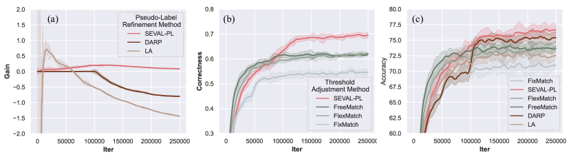
Figure 3: (a) The evolution of Gain across training iterations. SEVAL accumulates a higher accuracy of pseudo-label than its counterparts. (b) The evolution of Correctness across training iterations. SEVAL can build better trade-off between quality and quantity. (c) The evolution of test accuracy across training iterations. SEVAL-PL outperforms other pseudo-label refinement methods.

In order to comprehensively and quantitatively investigate the accuracy of pseudo-label refined by different approaches, here we define $G$ as the sum of accuracy gain and balanced accuracy gain of pseudo-label over training iterations. Both sample-wise accuracy and class-wise accuracy are crucial measures for evaluating the quality of pseudo-labels. A low sample-specific accuracy can lead to noisier pseudo-labels, adversely affecting model performance. Meanwhile, a low class-specific accuracy often indicates a bias towards the dominant classes. Therefore, we propose a metric $G$ which is the combination of these two metrics. Specifically, given the pseudo-label $\hat{y}_{i}$ and predicted class $y_{i}^{\prime}$ of unlabelled dataset $\mathcal{U}$, we calculate $G$ as:

$$G=\underbrace{\frac{\sum_{i=1}^{M}[{\mathbbm{1}(\hat{y}_{i}^{\prime}=y_{i})}-{\mathbbm{1}(\hat{y}_{i}=y_{i})]}}{M}}_{\text{Sample-Wise Accuracy Gain}}+\underbrace{\sum_{c=1}^{C}\sum_{i=1}^{M}\frac{\mathbbm{1}(\hat{y}_{i}^{\prime}=c)\mathbbm{1}(\hat{y}_{i}^{\prime}=y_{i})-\mathbbm{1}(\hat{y}_{i}=c)\mathbbm{1}(\hat{y}_{i}=y_{i})}{m_{c}C}}_{\text{Class-Wise Accuracy Gain}}.$$ (9)

To evaluate the cumulative impact of pseudo-labels, we calculate $\textbf{Gain}(\textbf{iter})$ as the accuracy gain at training iteration iter and monitor $\textbf{Gain}(\textbf{iter})=\sum_{j=1}^{\textbf{iter}}G(j)/\textbf{iter}$ throughout the training iterations. The results of SEVAL along with DARP and adjusting pseudo-label logit $\hat{z}_{c}^{\mathcal{U}}$ with LA are summarized in Fig. 3(a). We note that SEVAL consistently delivers a positive Gain throughout the training iterations. In contrast, DARP and LA tend to reduce the accuracy of pseudo-labels during the later stages of the training process. After a warm-up period, DARP adjusts the distribution of pseudo-labels to match the inherent distribution of unlabelled data. However, it doesn’t guarantee the accuracy of the pseudo-labels, thus not optimal. While LA can enhance class-wise accuracy, it isn’t always the best fit for every stage of the model’s learning. Consequently, noisy pseudo-labels from the majority class can impede the model’s training. SEVAL learns a smooth curriculum of parameters for pseudo-label refinement from the data itself, therefore bringing more stable improvements. We can further validate the effectiveness of SEVAL from the test accuracy curves shown in Fig. 3(c) where SEVAL-PL outperforms LA and DARP.

5.4.2 Threshold Adjustment

Quantity and quality are two essential factors for pseudo-labels, as highlighted in Chen et al. (2023). Quantity refers to the number of correctly labeled samples produced by pseudo-label algorithms, while quality indicates the proportion of correctly labeled samples after applying confidence-based thresholding. In order to access the effectiveness of pseudo-label, we propose a metric called Correctness, which is a combination of quantity and quality. Having just high quantity or just high quality isn’t enough for effective pseudo-labels. For instance, setting exceedingly high thresholds might lead to the selection of a limited number of accurately labelled samples (high quality). However, this is not always the ideal approach, and the opposite holds true for quantity. Therefore, we propose a metric Correctness which combine quality and quantity. In particular, factoring in the potential imbalance of unlabelled data, we utilize a class frequency based weight term $\bm{\omega}^{\mathcal{U}}=1/\bm{m}$ to normalize this metric, yielding:

$$\textbf{Correctness}=\underbrace{\frac{\mathcal{C}}{\sum_{i=1}^{M}\omega^{\mathcal{U}}_{y_{i}}}}_{\text{Quantity}}\underbrace{\frac{\mathcal{C}}{\sum_{i=1}^{M}{\omega^{\mathcal{U}}_{y_{i}}\mathbbm{1}(\max_{j}({q}_{ij})\geq\tau_{y_{i}^{\prime}})}}}_{\text{Quality}},$$ (10)

where, $\mathcal{C}=\sum_{i=1}^{M}\omega^{\mathcal{U}}_{y_{i}}{\mathbbm{1}(\hat{y}_{i}=y_{i})}{\mathbbm{1}(\max_{j}({q}_{ij})\geq\tau_{y_{i}^{\prime}})}$ is the relative number of correctly labelled samples. We show Correctness of SEVAL with FixMatch, FlexMatch and FreeMatch in Fig. 3(a). We observe that FlexMatch and FreeMatch can both improve Correctness, while SEVAL can boost even more. We observe that the test accuracy follows a trend similar to Correctness, as shown in Fig. 3(b). This demonstrates that the thresholds set by SEVAL not only ensure a high quantity but also attain high accuracy for pseudo-labels, making them efficient in the model’s learning process.

5.5 Ablation Study

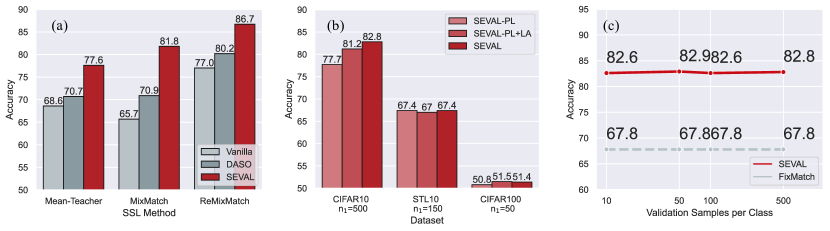
Figure 4: (a) Test accuracy when SEVAL is adapted to pseudo-label based SSL algorithms other than FixMatch under the setting of CIFAR-10 $n_{1}=1500$. SEVAL can readily improve the performance of other SSL algorithsm. (b) Test accuracy when SEVAL employs varied types of post-hoc adjustment parameters. The learned post-hoc parameters consistently enhance performance, particularly in CIFAR-10 experiments. (c) Test accuracy when SEVAL is optimized using different validation samples under the setting of CIFAR-10 $n_{1}=500$. SEVAL requires few validation samples to learn the optimal curriculum of parameters.

5.5.1 Flexibility and Compatibility

We apply SEVAL to other pseudo-label based SSL algorithms including Mean-Teacher, MixMatch and ReMixMatch and report the results with the setting of CIFAR-100 $n_{1}=50$ in Fig. 4(a). We find SEVAl can bring substantial improvements to these methods and is more effective than DASO. Of note the results of ReMixMatch w/SEVAL is higher than the results of FixMatch w/ SEVAL in Table 2 (86.7 vs 85.3). This may indicates that ReMixMatch is fit imbalanced SSL better. Due to its simplicity, SEVAL can be readily combined with other SSL algorithms that focus on LTL instead of PLR and THA. For example, SEVAL pairs effectively with the semantic alignment regularization introduced by DASO. By incorporating this loss into our FixMatch experiments with SEVAL, we were able to boost the test accuracy from 51.4 to 52.4 using the CIFAR-100 $n_{1}=50$ configuration.

We compare with the post-hoc adjustment process with LA in Fig. 4(b). We find that those post-hoc parameters can improve the model performance in the setting of CIFAR-10. In other cases, our post-hoc adjustment doesn’t lead to a decrease in prediction accuracy. However, LA sometimes does, as seen in the case of STL-10. This could be due to the complexity of the confusion matrix in those instances, where the class bias is not adequately addressed by simple offsets.

5.5.2 Data-Efficiency

Here we explore if SEVAL requires a substantial number of validation samples for curriculum learning. To do so, we keep the training dataset the same and optimize SEVAL parameters using balanced validation dataset with varied numbers of labelled samples using the CIFAR-10 $n_{1}=500$ configuration, as shown in Fig. 4(c). We find that SEVAL consistently identifies similar $\bm{\pi}$ and $\bm{\tau}$. When we train the model using these curricula, there aren’t significant differences even when the validation samples per class ranges from 10 to 500. This suggests that SEVAL is both data-efficient and resilient. We conduct stress tests on SEVAL and observe its effectiveness, even with only 40 labelled samples in total, as detailed in the Section 5.3.

5.6 Analysis of Learned Thresholds

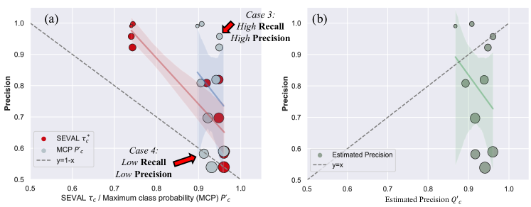
Figure 5: The correlation of different metrics between test Precision of FixMatch on CIFAR10-LT $n_{1}=500$. (a) The correlation of SEVAL learned $\tau_{c}$ and maximum class probability $P^{\prime}_{c}$ between test Precision. Each point represents a class c and the size of the points indicate the number of samples in the labelled training dataset $n_{c}$. Note that maximum class probability $P^{\prime}_{c}$ is the basis of current dynamic threshold method to derive thresholds. For example, FlexMatch selects more samples for classes associated with lower $P^{\prime}_{c}$. However, as highlighted by red arrows, $P^{\prime}_{c}$ does not correlated with Precision thus $P_{c}$ based on methods will fail Case 3: High Recall $\&$ High Precision and Case 4: Low Recall $\&$ Low Precision in Fig. 1. (b) Due to the lack of calibration in the network output probability, the estimated precision derived from the probability does not align with the actual Precision, thus cannot be a reliable metric to derive thresholds.

We try to determine the effectiveness of thresholds by looking into Precision of different classes, which should serve as approximate indicators of suitable thresholds. We illustrate an example of optimized thresholds and the learning status of FixMatch on CIFAR10-LT $n_{1}=500$ in Fig. 5(a), where SEVAL learns $\tau_{c}$ to be low for classes that have high Precision. In contrast, maximum class probability $P^{\prime}_{c}$, does not show clear correction with Precision. Specifically, as highlighted with the red arrows, $P_{c}$ remains high for classes that exhibit high Precision. Consequently, maximum class probability-based threshold methods such as FlexMatch will tune the threshold to be high for classes with large $P_{c}$, inadequately addressing Case 3 and Case 4 as elaborated in Section 3.

Instead of depending on an independent labelleddataset, we also attempt to estimate Precision using the model probability, so as to leverage the estimated precision to determine the appropriate thresholds. Specifically, we estimate the Precision of class $c$ as:

$$Q^{\prime}_{c}=\frac{\sum_{i=1}^{K}\mathbbm{1}_{ic}\max_{j}{p}_{ij}^{\mathcal{U}}}{\sum_{i=1}^{K}{p}_{ic}^{\mathcal{U}}}.$$ (11)

We visualize the estimated precision in Fig. 5(b). We find the the estimated precision does not align with the actual Precision. This is because the model is uncalibrated and the $Q^{\prime}_{c}$ is heavily decided by the true positives parts (e.g. numerator in Eq. 11), thus cannot reflect the real model precision. Thus it is a essential to utilize a holdout labelled dataset to derive the optimal thresholds.

Finally, we look into the class-wise performance of SEVAL and its counterparts in Fig 6. When compared with alternative methods, SEVAL achieves overall better performance with higher Recall on minority classes and higher Precision on majority classes. In this case, class 6 falls into Case 3: High Recall $\&$ High Precision while class 5 falls into Case 4: Low Recall $\&$ Low Precision. SEVAL shows advantages on these classes.

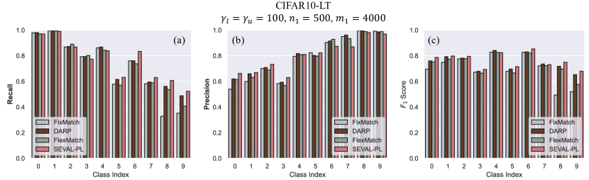
Figure 6: Class-wise performance for different SSL methods. Class indexes are arranged in descending order according to their class frequencies. We find that SEVAL achieve better overall performance than its counterparts by making neural networks more sensitive to minority classes.

6 Conclusion and Future Work

In this study, we present SEVAL and highlight its benefits in imbalanced SSL across a wide range of application scenarios. SEVAL sheds new light on pseudo-label generalization, which is a foundation for many leading SSL algorithms. SEVAL is both straightforward and potent, requiring no extra computation once the curriculum is acquired. As such, it can be effortlessly integrated into other SSL algorithms and paired with LTL methods to address class imbalance. We believe that the concept of optimizing parameters or accessing unbiased learning status using a partition of the labeled training dataset could spark further innovations in long-tailed recognition and SSL. We feel that the specific interplay between label refinement and threshold adjustment remains an intriguing question for subsequent research.

In the future, by leveraging Bayesian or bootstrap techniques, we may eliminate the need for internal validation in SEVAL by improving model calibration Loh et al. (2022); Vucetic and Obradovic (2001). We also plan to analyze SEVAL within the theoretical framework of SSL Mey and Loog (2022) to acquire deeper insights.

Acknowledgments and Disclosure of Funding

SJ is supported by a Wellcome Senior Research Fellowship (221933/Z/20/Z) and a Wellcome Collaborative Award (215573/Z/19/Z). The Wellcome Centre for Integrative Neuroimaging is supported by core funding from the Wellcome Trust (203139/Z/16/Z). The computational aspects of this research were partly carried out at Oxford Biomedical Research Computing (BMRC), which is funded by the NIHR Oxford BRC with additional support from the Wellcome Trust Core Award Grant Number 203141/Z/16/Z.

Appendix

Appendix A Proofs

A.1 Proof of Proposition 1

$$f_{\mathcal{T}}(X)=P_{\mathcal{T}}(Y|X)$$ (12)

$$=\frac{P_{\mathcal{T}}(X|Y)P_{\mathcal{T}}(Y)}{P_{\mathcal{T}}(X)},$$

when we assume there does not exist conditional shifts between training and test dataset following Saerens et al. (2002), e.g. $P_{\mathcal{X}}(X|Y)=P_{\mathcal{T}}(X|Y)$, we can rewrite Eq. 12 as:

$$\frac{P_{\mathcal{T}}(X|Y)P_{\mathcal{T}}(Y)}{P_{\mathcal{T}}(X)}=\frac{P_{\mathcal{T}}(X|Y)P_{\mathcal{T}}(Y)}{P_{\mathcal{T}}(X)}\cdot\frac{P_{\mathcal{X}}(X)}{P_{\mathcal{X}}(X)}$$ (13)

$$\quad\quad\quad\quad\propto\frac{P_{\mathcal{X}}(X|Y)P_{\mathcal{T}}(Y)}{P_{\mathcal{X}}(X)}$$

$$\quad\quad\quad\quad=\frac{P_{\mathcal{X}}(X,Y)P_{\mathcal{T}}(Y)}{P_{\mathcal{X}}(X)P_{\mathcal{X}}(Y)}$$

$$\quad\quad\quad\quad=\frac{P_{\mathcal{X}}(Y|X)P_{\mathcal{T}}(Y)}{P_{\mathcal{X}}(Y)}$$

$$\quad\quad\quad\quad=\frac{f^{*}(X)P_{\mathcal{T}}(Y)}{P_{\mathcal{X}}(Y)}.$$

$\blacksquare$

A.2 Proof of Theorem 3

We derive the generalization bound based on the Rademacher complexity method Bartlett and Mendelson (2002) following the analysis for noisy label training Natarajan et al. (2013); Liu and Tao (2015).

Lemma 5

We define:

$$\hat{\mathcal{L}}(\cdot,y):=\frac{(1-\rho)\mathcal{L}(\cdot,y)-\rho\mathcal{L}(\cdot,3-y)}{1-2\rho}.$$ (14)

With this loss function, we should have:

$$\mathbb{E}_{\hat{y}}[\hat{\mathcal{L}}(\cdot,\hat{y})]=\mathcal{L}(\cdot,y).$$ (15)

Given $\hat{R}_{\hat{\mathcal{L}},\hat{\mathcal{U}}}(f):=\frac{1}{M}\sum_{i=1}^{M}\hat{\mathcal{L}}(f(\bm{u}_{i}),\hat{y}_{i})$ the empirical risk on $\hat{\mathcal{U}}$ and $R_{\hat{\mathcal{L}},\hat{\mathcal{U}}}(f)$ is the corresponding expected risk, we have the basic generalization bound as:

$$\max_{f\in\mathcal{F}}|\hat{R}_{\hat{\mathcal{L}},\hat{\mathcal{U}}}(f)-R_{\hat{\mathcal{L}},\hat{\mathcal{U}}}(f)|\leq 2\mathfrak{R}(\hat{\mathcal{L}}\circ\mathcal{F})+\sqrt{\frac{\log(1/\delta)}{2M}},$$ (16)

where:

$$\mathfrak{R}(\hat{\mathcal{L}}\circ\mathcal{F}):=\mathbb{E}_{\bm{u}_{i},\hat{y}_{i},\epsilon_{i}}\left[\sup_{f\in\mathcal{F}}\frac{1}{M}\sum_{i=1}^{M}\epsilon_{i}\hat{\mathcal{L}}(f(\bm{u}_{i}),\hat{y}_{i})\right].$$ (17)

If $\mathcal{L}$ is $L$-Lipschitz then $\hat{\mathcal{L}}$ is $L_{\rho}$ Lipschitz with:

$$L_{\rho}=\frac{L}{1-2\rho}.$$ (18)

Based on Talagrand’s Lemma Mohri et al. (2018), we have:

$$\mathfrak{R}(\hat{\mathcal{L}}\circ\mathcal{F})\leq L_{\rho}\mathfrak{R}(\mathcal{F}),$$ (19)

where $\mathfrak{R}(\mathcal{F}):=\mathbb{E}_{\bm{x}_{i},\epsilon_{i}}\left[\sup_{f\in\mathcal{F}}\frac{1}{M}\sum_{i=1}^{M}\epsilon_{i}f(\bm{u}_{i})\right]$ is the Rademacher complexity for function class $\mathcal{F}$ and $\epsilon_{1},\ldots,\epsilon_{M}$ are i.i.d. Rademacher variables.

Let $\hat{f}$ be the model after optimizing with $\hat{\mathcal{U}}$, and let $f^{*}$ be the minimization of the expected risk $R_{\mathcal{L},\mathcal{U}}$ over $\mathcal{F}$. Then, we have:

$$R_{\mathcal{L},\mathcal{U}}(\hat{f})-R_{\mathcal{L},\mathcal{U}}(f^{*})$$ (20)

$$=R_{\hat{\mathcal{L}},\hat{\mathcal{U}}}(\hat{f})-R_{\hat{\mathcal{L}},\hat{\mathcal{U}}}(f^{*})$$

$$=\big{(}\hat{R}_{\hat{\mathcal{L}},\hat{\mathcal{U}}}(\hat{f})-\hat{R}_{\hat{\mathcal{L}},\hat{\mathcal{U}}}(f^{*})\big{)}+$$

$$\quad\big{(}\hat{R}_{\hat{\mathcal{L}},\hat{\mathcal{U}}}(f^{*})-R_{\hat{\mathcal{L}},\hat{\mathcal{U}}}(f^{*})\big{)}+\big{(}R_{\hat{\mathcal{L}},\hat{\mathcal{U}}}(\hat{f})-\hat{R}_{\hat{\mathcal{L}},\hat{\mathcal{U}}}(\hat{f})\big{)}$$

$$\leq 0+2\max_{f\in\mathcal{F}}|\hat{R}_{\hat{\mathcal{L}},\hat{\mathcal{U}}}(f)-R_{\hat{\mathcal{L}},\hat{\mathcal{U}}}(f)|$$

After we combine Eq. 16 and Eq. 20, we obtain the bound described in Theorem 3. $\blacksquare$

A.3 Proof of Lemma 5

Based on Eq. 15, we calculate the cases for $y=1$ and $y=2$ and obtain:

$$(1-\rho)\hat{\mathcal{L}}(\cdot,1)+\rho\hat{\mathcal{L}}(\cdot,2)=\mathcal{L}(\cdot,1),$$ (21)

$$(1-\rho)\hat{\mathcal{L}}(\cdot,2)+\rho\hat{\mathcal{L}}(\cdot,1)=\mathcal{L}(\cdot,2).$$ (22)

By solving the two equations, we yield:

$$\hat{\mathcal{L}}(\cdot,1)=\frac{(1-\rho)\mathcal{L}(\cdot,1)-\rho\mathcal{L}(\cdot,2)}{1-2\rho},$$ (23)

$$\hat{\mathcal{L}}(\cdot,2)=\frac{(1-\rho)\mathcal{L}(\cdot,2)-\rho\mathcal{L}(\cdot,1)}{1-2\rho}.$$ (24)

$\blacksquare$

Appendix B Additional Experiments

In this section, we present additional experimental results conducted under various settings to assess the generalizability of SEVAL.

B.1 Sensitivity Analysis

We perform experiments with SEVAL, varying the core hyperparameters, and present the results in Table 7. Our findings indicate that SEVAL exhibits robustness, showing insensitivity to hyper-parameter variations within a reasonable range.

	CIFAR10-LT, $\gamma_{l}=100$
Hyper-parameter	$n_{1}=500$, $m_{1}=4000$
$t=0.6$	82.5$\,\pm$0.45
$t=0.7$	82.2$\,\pm$0.11
$t=0.75$  (reported)	82.8$\,\pm$0.56
$\eta_{\pi}=0.995$	81.4$\,\pm$0.36
$\eta_{\pi}=0.999$  (reported)	82.8$\,\pm$0.56
$\eta_{\pi}=0.9995$	82.5$\,\pm$0.35
$\eta_{\tau}=0.995$	81.5$\,\pm$0.38
$\eta_{\tau}=0.999$  (reported)	82.8$\,\pm$0.56
$\eta_{\tau}=0.9995$	82.9$\,\pm$0.09

Table 7: Sensitivity analysis of hyper-parameters $t$, $\eta_{\pi}$ and $\eta_{\tau}$. Best results are in bold for each configuration.

B.2 Results on ImageNet-127

	Method type			Small- ImageNet-127
Algorithm	LTL	PLR	THA
FixMatch				29.4
w/ FreeMatch		✓	✓	30.0
w/ SEVAL-PL		✓	✓	31.0
w/ SAW	✓			29.4
w/ DASO	✓	✓		29.4
w/ SEVAL	✓	✓	✓	34.8

Table 8: Averaged class recall on Small-ImageNet-127. Best results within the same category are in bold for each configuration.

We conduct experiments on Small ImageNet-127 Su and Maji (2021) with a reduced image size of 32 $\times$ 32 following Fan et al. (2022). ImageNet-127 consolidates the 1000 classes of ImageNet into 127 categories according to the WordNet hierarchy. This results in a naturally long-tailed class distribution with an imbalance ratio of $\gamma_{l}=\gamma_{u}=286$. We randomly select 10$\%$ of the training samples as the labeled set and utilize the remainder as unlabeled data. We conduct experiments using ResNet-50 and Adam optimizer. Results are summarized in Table 8.

B.3 Integration with Other SSL Frameworks

As an extension to results in Fig. 4, we summarize the results when introducing SEVAL into other SSL frameworks in Table 9. We summarize the implementation details of those methods in Section C.

	CIFAR10-LT	CIFAR100-LT
Algorithm	$n_{1}=1500$, $m_{1}=3000$	$n_{1}=150$, $m_{1}=300$
	$\gamma_{l}=\gamma_{u}=100$	$\gamma_{l}=\gamma_{u}=10$
Mean Teacher Tarvainen and Valpola (2017)	68.6$\,\pm$0.88	52.1$\,\pm$0.09
w/ DASO Oh et al. (2022)	70.7$\,\pm$0.59	52.5$\,\pm$0.37
w/ SEVAL	77.6$\,\pm$0.63	53.8$\,\pm$0.24
MixMatch Berthelot et al. (2019b)	65.7$\,\pm$0.23	54.2$\,\pm$0.47
w/ DASO Oh et al. (2022)	70.9$\,\pm$1.91	55.6$\,\pm$0.49
w/ SEVAL	81.8$\,\pm$0.82	57.8$\,\pm$0.26
ReMixMatch Berthelot et al. (2019a)	77.0$\,\pm$0.55	61.5$\,\pm$0.57
w/ DASO Oh et al. (2022)	80.2$\,\pm$0.68	62.1$\,\pm$0.69
w/ SEVAL	86.7$\,\pm$0.71	63.1$\,\pm$0.38

Table 9: Accuracy on CIFAR10-LT based on SSL methods other than FixMatch. Best results within the same category are in bold for each configuration.

Appendix C Implementation Details

C.1 Learning with Imbalanced Validation Data

As the labelled training dataset $\mathcal{X}$ is imbalanced, in practice, it is hard to obtain a balanced split $\mathcal{V}$ to learn a curriculum of threshold $\bm{\tau}$. However, when we optimize $\bm{\tau}$ using an imbalanced validation $\mathcal{V}$ following Eq. 7, the optimized results would be biased. More precisely, the majority class consistently exhibits high Precision, leading to a lower threshold, while the opposite holds true for the minority class. Therefore, we utilize the class frequency of the labelled validation data $\bm{k}$ to normalize the cost function. Specifically, we calculate the class weight as $\bm{\omega}^{\mathcal{V}}=1/\bm{k}$. This parameter would assign large weight to the minority class and small weight to the majority classes. Then we replace all the $\mathbbm{1}_{ic}$ with $\omega_{y_{i}}^{\mathcal{V}}\mathbbm{1}_{ic}$ in Eq. 7, obtaining:

$$\tau_{c}^{*}=\begin{cases}\operatorname*{arg\,min}_{\tau_{c}}\big{|}\frac{1}{s_{c}}\sum_{i=1}^{K}\omega_{y_{i}}^{\mathcal{V}}\mathbbm{1}_{ic}\mathbbm{1}(y_{i}=c)\mathbbm{1}(\max_{j}({p}_{ij}^{\mathcal{V}})>\tau_{c})-t\big{|}&\text{if}\quad t<\alpha_{c}\\ \quad\quad\quad\quad 0&\text{otherwise}\\ \end{cases},$$ (25)

where $s_{c}=\sum_{i=1}^{K}\omega_{y_{i}}^{\mathcal{V}}\mathbbm{1}_{ic}\mathbbm{1}(\max_{j}({p}_{ij}^{\mathcal{V}})>\tau_{c})$ is the relative number of samples predicted as class $c$ with confidence larger than $\tau_{c}$, where $\alpha_{c}=\frac{1}{K_{c}}\sum_{i=1}^{K}\omega_{y_{i}}^{\mathcal{V}}\mathbbm{1}_{ic}\mathbbm{1}(y_{i}=c)$ is the average balanced accuracy of all the samples predicted as class $c$ and $K_{c}=\sum_{i=1}^{K}\omega_{y_{i}}^{\mathcal{V}}\mathbbm{1}_{ic}$ is the relative number of samples predicted as $c$. This modification can normalize the number of samples within the cost function. Consequently, we can directly learn the thresholds $\bm{\tau}$ using imbalanced validation data.

C.2 Learning Thresholds within Groups

When we learn $\bm{\tau}$ based on the validation data $\mathcal{V}$, the optimization process could be unstable as sometimes we have very few samples per class (e.g. less than 10 samples). In this case, even if we can re-weight the validation samples based on their class prior $\bm{k}$, it is hard to have enough samples to obtain stable $\bm{\tau}$ curriculum for the minority classes, especially when $\min_{c}(k_{c})<10$. Assuming equal class priors should result in similar thresholds, we propose to optimize thresholds within groups, pinpointing the ideal ones that fulfill the accuracy requirement for every classes within the group.

We assume the samples of different classes $k_{c}$ are arranged in descending order. In other words, $k_{1}$ is the maximum, and $k_{C}$ is the minimum. Instead of optimizing $\tau_{c}$ for an individual class $c$, we optimize for groups such that the learned $\tau_{b}$ can satisfy the accuracy requirements for $B$ classes. Specifically, the optimal $\tilde{\bm{\tau}}\in\mathbb{R}^{C/B}$ is determined as:

$$\tilde{\tau}_{b}^{*}=\begin{cases}\sum_{c=bB+1}^{bB+B}\operatorname*{arg\,min}_{\tilde{\tau}_{b}}\big{|}\frac{1}{\tilde{s}_{b}}\sum_{i=1}^{K}\mathbbm{1}_{ic}\mathbbm{1}(y_{i}=c)\mathbbm{1}(\max_{j}({p}_{ij}^{\mathcal{V}})>\tilde{\tau}_{b})-t\big{|}&\text{if}\quad t<\tilde{\alpha}_{b}\\ \quad\quad\quad\quad 0&\text{otherwise}\\ \end{cases},$$ (26)

where $\tilde{s}_{b}=\sum_{c=bB+1}^{bB+B}\sum_{i=1}^{K}\mathbbm{1}_{ic}\mathbbm{1}(\max_{j}({p}_{ij}^{\mathcal{V}})>\tilde{\tau}_{b})$ is the number of samples that are chosen in this group based on the threshold $\tilde{\tau}_{b}$ and $\tilde{\alpha}_{b}=\frac{1}{\sum_{c=bB+1}^{bB+B}K_{c}}\sum_{c=bB+1}^{bB+B}\sum_{i=1}^{K}\mathbbm{1}_{ic}\mathbbm{1}(y_{i}=c)$ is the average accuracy of all the samples predicted as class in this group. If we set $B=1$, Eq. 26 becomes equivalent to Eq. 7.

Furthermore, in practice, we find that in the setting of imbalanced SSL, sometimes the minority classes very few samples and the thresholds cannot be optimized correctly based on Eq. 26. In this case, we also set the learned $\tilde{\tau}_{b}^{*}$ to be 0, in order to leverage more data from the minority classes. Formally, we denote $\tilde{K}_{b}=\sum_{c=bB+1}^{bB+B}\sum_{i=1}^{K}\omega_{y_{i}}^{\mathcal{V}}\mathbbm{1}_{ic}$ as the relative number of predicted samples within group $b$. When $\tilde{K}_{b}<\sum_{i=1}^{K}\frac{B\omega_{y_{i}}^{\mathcal{V}}}{e_{1}C}$ or $\sum_{i=1}^{K}\mathbbm{1}(y_{i}=c)<e_{2}$, where $e_{1}$ and $e_{2}$ are hyper-parameters that we both set to 10 for all experiments, we also have $\tilde{\tau}_{b}^{*}=0$ and keep their corresponding $\pi_{c}$ within group $b$ as low as $\pi_{c}=\min_{j}(\pi_{j})$. This implies:

• In instances where the models exhibit a pronounced bias, limiting their capability to detect over 10$\%$ of the samples within a particular group, we adjust the associated thresholds and consequently increase our sample selection.

• When a group comprises fewer than 10 samples, the feasibility of optimizing thresholds based on proportion diminishes, necessitating an enhanced sample selection.

C.3 Benchmarks

We conduct experiments upon the code base of Oh et al. (2022) for experiments of CIFAR10-LT, CIFAR100-LT and STL10-LT. We take some baseline results from the DASO paper Oh et al. (2022) to Table 2, Table 4 and Table 9. including the results of supervised baselines, DARP, CReST+, ABC and DASO.

As DASO Oh et al. (2022) does not supply the code for the Semi-Aves experiments, we conduct all the experiments for this setting ourselves. We train ResNet-50 He et al. (2016) which is pretrained on ImageNet Deng et al. (2009) for the task of Semi-Aves following Su and Maji (2021). In accordance with Oh et al. (2022), we merge the training and validation datasets provided by the challenge, yielding a total of 5,959 samples for training which come from 200 classes. We conduct experiments utilizing 26,640 unlabelled samples which share the same label space with $\mathcal{X}$ in the $\mathcal{U}=\mathcal{U}_{in}$ setting, and 148,848 unlabelled samples of which 122,208 are from open-set classes in the $\mathcal{U}=\mathcal{U}_{in}+\mathcal{U}_{out}$ setting. For experiments on Semi-Aves, we set the base learning rate as 0.005. We train the network for 45,000 iterations. The learning rate is linear warmed up during the first 25,00 iterations, and degrade after 15,000 and 30,000, with a factor of 10. We choose training batch size as 32. The images are firstly cropped to $256\times 256$. During training, the images are then randomly cropped to $224\times 224$. At inference time, the images are cropped in the center with size $224\times 224$.

C.4 Hyper-Parameters

Here we summarize all the hyper-parameters we choose in this experiments to ease reproducibility.

Hyper-parameter	CIFAR10-LT, $\gamma_{l}=100$		CIFAR100-LT, $\gamma_{l}=10$		STL10-LT, $\gamma_{l}=20$		Semi-Aves
	$n_{1}=500$	$n1=1500$	$n_{1}=50$	$n_{1}=150$	$n_{1}=150$	$n_{1}=450$	$\mathcal{U}=\mathcal{U}_{\text{in}}$	$\mathcal{U}=\mathcal{U}_{\text{in}}+\mathcal{U}_{\text{out}}$
	$m_{1}=4000$	$m_{1}=3000$	$m_{1}=400$	$m_{1}=300$	$M=100,000$
$C$	10		100		10		200
$T$	250,000		250,000		250,000		45,000
$t$	0.75		0.5	0.65	0.7	0.6	0.9	0.99
${\color[rgb]{.5,.5,.5}t^{\mathcal{V}}}$	0.9		0.65	0.7	0.95	0.85	—–
$L$	500		100		500		90
$B$	2		25	10	2	1	10
$\eta_{\pi}$	0.999		0.95	0.9	0.995		0.99	0.9
$\eta_{\tau}$	0.999		0.95	0.9	0.9995	0.999	0.99	0.9

Table 10: Experiment-specific hyper-parameters. $t^{\mathcal{V}}$ is the required accuracy if we directly optimize $\bm{\tau}$ along the training process using a separate validation dataset.

C.5 SEVAL with Other SSL Algorithms

Here, we provide implementation details of how SEVAL can be integrated into other pseudo-labeling based SSL algorithms. Specifically, we apply SEVAL to Mean Teacher Tarvainen and Valpola (2017), MixMatch Berthelot et al. (2019b) and ReMixMatch Berthelot et al. (2019a). These algorithms produce pseudo-label $\hat{y}_{i}$ based on its corresponding pseudo-label probability $\bm{q}_{i}$ and logit $\hat{\bm{z}}_{i}^{\mathcal{U}}$ in different ways. SEVAL can be easily adapted by refining $\bm{q}_{i}$ using the learned offset $\bm{\pi}^{*}$.

It should be noted that these SSL algorithms do not include the process of filtering out pseudo-labels with low confidence. Therefore, for simplicity and fair comparison, we do not include the threshold adjustment into these methods. We expect that SEVAL can further enhance performance through threshold adjustment and plan to explore this further in the future.

C.5.1 Mean Teacher

Mean Teacher generates pseudo-label logit $\hat{\bm{z}}_{i}^{\mathcal{U}}$ based on a EMA version of the prediction models. SEVAL calculates the pseudo-label probability as $\bm{q}_{i}=\sigma(\hat{\bm{z}}_{i}^{\mathcal{U}}-\log\bm{\pi}^{*})$, which is expected to have less bias towards the majority class.

C.5.2 MixMatch

MixMatch calculates $\hat{y}_{i}$ based on multiple transformed version of an unlabelled sample $\bm{u}_{i}$. SEVAL adjusts each one of them with $\bm{\pi}^{*}$, separately.

C.5.3 ReMixMatch

ReMixMatch proposes to refine pseudo-label probability $\bm{q}_{i}$ with distribution alignment to match the marginal distributions. SEVAL adjusts the the probability using $\bm{q}_{i}=\sigma(\hat{\bm{z}}_{i}^{\mathcal{U}}-\log\bm{\pi}^{*})$ before ReMixMatch’s process including distribution alignment and temperature sharpening.

Appendix D Classes of Different Performance

Here we summarize the number of classes of different performance, as demonstrated in Fig. 1. We report the model performance of FixMatch trained on different datasets. Here we consider a class to have high Recall when its performance surpasses the average Recall of the classes. The same principle applies to Precision. We observe that $Case1$ is frequently encountered in the majority class, while $Case2$ is commonly observed in the minority class. $Case3$ and $Case4$ also widely exist in different scenarios. The threshold learning strategies in SEVAL fits $Case3$ and $Case4$, thus perform better.

	CIFAR10-LT		CIFAR100-LT		STL10-LT		Semi-Aves
	$\gamma_{l}=\gamma_{u}=100$		$\gamma_{l}=\gamma_{u}=10$		$\gamma_{l}=20$, $\gamma_{u}$: unknown
Model Performance	$n_{1}=500$	$n_{1}=1500$	$n_{1}=50$	$n_{1}=150$	$n_{1}=150$	$n_{1}=450$	$\mathcal{U}=\mathcal{U}_{\text{in}}$	$\mathcal{U}=$
	$m_{1}=4000$	$m_{1}=3000$	$m_{1}=400$	$m_{1}=300$	$M=100,000$			$\mathcal{U}_{\text{in}}+\mathcal{U}_{\text{out}}$
Case 1: High Recall $\&$ Low Precision	4	5	24	29	2	4	36	45
Case 2: Low Recall $\&$ High Precision	4	4	18	20	2	2	35	45
Case 3: High Recall $\&$ High Precision	1	1	33	29	3	2	69	58
Case 4: Low Recall $\&$ Low Precision	1	0	25	22	3	2	60	52
Total classes	10	10	100	100	10	10	200	200

Table 11: The number of classes of different performance when trained with FixMatch. We demonstrate the prevalent occurrence of the four class performance scenarios in existing semi-supervised learning tasks.

References

- Bartlett and Mendelson (2002) Peter L Bartlett and Shahar Mendelson. Rademacher and gaussian complexities: Risk bounds and structural results. Journal of Machine Learning Research, 3(Nov):463–482, 2002.
- Berthelot et al. (2019a) David Berthelot, Nicholas Carlini, Ekin D Cubuk, Alex Kurakin, Kihyuk Sohn, Han Zhang, and Colin Raffel. Remixmatch: Semi-supervised learning with distribution alignment and augmentation anchoring. arXiv preprint arXiv:1911.09785, 2019a.
- Berthelot et al. (2019b) David Berthelot, Nicholas Carlini, Ian Goodfellow, Nicolas Papernot, Avital Oliver, and Colin A Raffel. Mixmatch: A holistic approach to semi-supervised learning. Advances in neural information processing systems, 32, 2019b.
- Bridle et al. (1991) John Bridle, Anthony Heading, and David MacKay. Unsupervised classifiers, mutual information and’phantom targets. Advances in neural information processing systems, 4, 1991.
- Cao et al. (2019) Kaidi Cao, Colin Wei, Adrien Gaidon, Nikos Arechiga, and Tengyu Ma. Learning imbalanced datasets with label-distribution-aware margin loss. Advances in neural information processing systems, 32, 2019.
- Chapelle et al. (2009) Olivier Chapelle, Bernhard Scholkopf, and Alexander Zien. Semi-supervised learning (chapelle, o. et al., eds.; 2006)[book reviews]. IEEE Transactions on Neural Networks, 20(3):542–542, 2009.
- Chawla et al. (2002) Nitesh V Chawla, Kevin W Bowyer, Lawrence O Hall, and W Philip Kegelmeyer. Smote: synthetic minority over-sampling technique. Journal of artificial intelligence research, 16:321–357, 2002.
- Chen et al. (2022) Hao Chen, Yue Fan, Yidong Wang, Jindong Wang, Bernt Schiele, Xing Xie, Marios Savvides, and Bhiksha Raj. An embarrassingly simple baseline for imbalanced semi-supervised learning. arXiv preprint arXiv:2211.11086, 2022.
- Chen et al. (2023) Hao Chen, Ran Tao, Yue Fan, Yidong Wang, Jindong Wang, Bernt Schiele, Xing Xie, Bhiksha Raj, and Marios Savvides. Softmatch: Addressing the quantity-quality trade-off in semi-supervised learning. arXiv preprint arXiv:2301.10921, 2023.
- Coates et al. (2011) Adam Coates, Andrew Ng, and Honglak Lee. An analysis of single-layer networks in unsupervised feature learning. In Proceedings of the fourteenth international conference on artificial intelligence and statistics, pages 215–223. JMLR Workshop and Conference Proceedings, 2011.
- Cubuk et al. (2020) Ekin D Cubuk, Barret Zoph, Jonathon Shlens, and Quoc V Le. Randaugment: Practical automated data augmentation with a reduced search space. In Proceedings of the IEEE/CVF conference on computer vision and pattern recognition workshops, pages 702–703, 2020.
- Deng et al. (2009) Jia Deng, Wei Dong, Richard Socher, Li-Jia Li, Kai Li, and Li Fei-Fei. Imagenet: A large-scale hierarchical image database. In 2009 IEEE conference on computer vision and pattern recognition, pages 248–255. Ieee, 2009.
- Fan et al. (2022) Yue Fan, Dengxin Dai, Anna Kukleva, and Bernt Schiele. Cossl: Co-learning of representation and classifier for imbalanced semi-supervised learning. In Proceedings of the IEEE/CVF conference on computer vision and pattern recognition, pages 14574–14584, 2022.
- Garg et al. (2022) Saurabh Garg, Sivaraman Balakrishnan, Zachary C Lipton, Behnam Neyshabur, and Hanie Sedghi. Leveraging unlabeled data to predict out-of-distribution performance. arXiv preprint arXiv:2201.04234, 2022.
- Gong et al. (2023) Shizhan Gong, Cheng Chen, Yuqi Gong, Nga Yan Chan, Wenao Ma, Calvin Hoi-Kwan Mak, Jill Abrigo, and Qi Dou. Diffusion model based semi-supervised learning on brain hemorrhage images for efficient midline shift quantification. In International Conference on Information Processing in Medical Imaging, pages 69–81. Springer, 2023.
- Grandvalet and Bengio (2004) Yves Grandvalet and Yoshua Bengio. Semi-supervised learning by entropy minimization. Advances in neural information processing systems, 17, 2004.
- Guo et al. (2017) Chuan Guo, Geoff Pleiss, Yu Sun, and Kilian Q Weinberger. On calibration of modern neural networks. In International conference on machine learning, pages 1321–1330. PMLR, 2017.
- Guo and Li (2022) Lan-Zhe Guo and Yu-Feng Li. Class-imbalanced semi-supervised learning with adaptive thresholding. In International Conference on Machine Learning, pages 8082–8094. PMLR, 2022.
- He et al. (2021) Ju He, Adam Kortylewski, Shaokang Yang, Shuai Liu, Cheng Yang, Changhu Wang, and Alan Yuille. Rethinking re-sampling in imbalanced semi-supervised learning. arXiv preprint arXiv:2106.00209, 2021.
- He et al. (2016) Kaiming He, Xiangyu Zhang, Shaoqing Ren, and Jian Sun. Deep residual learning for image recognition. In Proceedings of the IEEE conference on computer vision and pattern recognition, pages 770–778, 2016.
- Ho et al. (2019) Daniel Ho, Eric Liang, Xi Chen, Ion Stoica, and Pieter Abbeel. Population based augmentation: Efficient learning of augmentation policy schedules. In International conference on machine learning, pages 2731–2741. PMLR, 2019.
- Iscen et al. (2019) Ahmet Iscen, Giorgos Tolias, Yannis Avrithis, and Ondrej Chum. Label propagation for deep semi-supervised learning. In Proceedings of the IEEE/CVF conference on computer vision and pattern recognition, pages 5070–5079, 2019.
- Kamnitsas et al. (2018) Konstantinos Kamnitsas, Daniel Castro, Loic Le Folgoc, Ian Walker, Ryutaro Tanno, Daniel Rueckert, Ben Glocker, Antonio Criminisi, and Aditya Nori. Semi-supervised learning via compact latent space clustering. In International conference on machine learning, pages 2459–2468. PMLR, 2018.
- Kang et al. (2019) Bingyi Kang, Saining Xie, Marcus Rohrbach, Zhicheng Yan, Albert Gordo, Jiashi Feng, and Yannis Kalantidis. Decoupling representation and classifier for long-tailed recognition. arXiv preprint arXiv:1910.09217, 2019.
- Kim et al. (2020) Jaehyung Kim, Youngbum Hur, Sejun Park, Eunho Yang, Sung Ju Hwang, and Jinwoo Shin. Distribution aligning refinery of pseudo-label for imbalanced semi-supervised learning. Advances in neural information processing systems, 33:14567–14579, 2020.
- Krizhevsky et al. (2009) Alex Krizhevsky, Geoffrey Hinton, et al. Learning multiple layers of features from tiny images. Technical report, 2009.
- Lai et al. (2022a) Zhengfeng Lai, Chao Wang, Sen-ching Cheung, and Chen-Nee Chuah. Sar: Self-adaptive refinement on pseudo labels for multiclass-imbalanced semi-supervised learning. In Proceedings of the IEEE/CVF Conference on Computer Vision and Pattern Recognition, pages 4091–4100, 2022a.
- Lai et al. (2022b) Zhengfeng Lai, Chao Wang, Henrry Gunawan, Sen-Ching S Cheung, and Chen-Nee Chuah. Smoothed adaptive weighting for imbalanced semi-supervised learning: Improve reliability against unknown distribution data. In International Conference on Machine Learning, pages 11828–11843. PMLR, 2022b.
- Laine and Aila (2016) Samuli Laine and Timo Aila. Temporal ensembling for semi-supervised learning. arXiv preprint arXiv:1610.02242, 2016.
- Lazarow et al. (2023) Justin Lazarow, Kihyuk Sohn, Chen-Yu Lee, Chun-Liang Li, Zizhao Zhang, and Tomas Pfister. Unifying distribution alignment as a loss for imbalanced semi-supervised learning. In Proceedings of the IEEE/CVF Winter Conference on Applications of Computer Vision, pages 5644–5653, 2023.
- Lee et al. (2013) Dong-Hyun Lee et al. Pseudo-label: The simple and efficient semi-supervised learning method for deep neural networks. In Workshop on challenges in representation learning, ICML, volume 3, page 896. Atlanta, 2013.
- Lee et al. (2021) Hyuck Lee, Seungjae Shin, and Heeyoung Kim. Abc: Auxiliary balanced classifier for class-imbalanced semi-supervised learning. Advances in Neural Information Processing Systems, 34:7082–7094, 2021.
- Li et al. (2017) Chongxuan Li, Taufik Xu, Jun Zhu, and Bo Zhang. Triple generative adversarial nets. Advances in neural information processing systems, 30, 2017.
- Li et al. (2024) Muyang Li, Runze Wu, Haoyu Liu, Jun Yu, Xun Yang, Bo Han, and Tongliang Liu. Instant: Semi-supervised learning with instance-dependent thresholds. Advances in Neural Information Processing Systems, 36, 2024.
- Li et al. (2020) Zeju Li, Konstantinos Kamnitsas, and Ben Glocker. Analyzing overfitting under class imbalance in neural networks for image segmentation. IEEE transactions on medical imaging, 40(3):1065–1077, 2020.
- Li et al. (2022) Zeju Li, Konstantinos Kamnitsas, Mobarakol Islam, Chen Chen, and Ben Glocker. Estimating model performance under domain shifts with class-specific confidence scores. In International Conference on Medical Image Computing and Computer-Assisted Intervention, pages 693–703. Springer, 2022.
- Lipton et al. (2018) Zachary Lipton, Yu-Xiang Wang, and Alexander Smola. Detecting and correcting for label shift with black box predictors. In International conference on machine learning, pages 3122–3130. PMLR, 2018.
- Liu and Tao (2015) Tongliang Liu and Dacheng Tao. Classification with noisy labels by importance reweighting. IEEE Transactions on pattern analysis and machine intelligence, 38(3):447–461, 2015.
- Liu et al. (2019) Ziwei Liu, Zhongqi Miao, Xiaohang Zhan, Jiayun Wang, Boqing Gong, and Stella X Yu. Large-scale long-tailed recognition in an open world. In Proceedings of the IEEE/CVF conference on computer vision and pattern recognition, pages 2537–2546, 2019.
- Loh et al. (2022) Charlotte Loh, Rumen Dangovski, Shivchander Sudalairaj, Seungwook Han, Ligong Han, Leonid Karlinsky, Marin Soljacic, and Akash Srivastava. On the importance of calibration in semi-supervised learning. arXiv preprint arXiv:2210.04783, 2022.
- Menon et al. (2020) Aditya Krishna Menon, Sadeep Jayasumana, Ankit Singh Rawat, Himanshu Jain, Andreas Veit, and Sanjiv Kumar. Long-tail learning via logit adjustment. arXiv preprint arXiv:2007.07314, 2020.
- Mey and Loog (2022) Alexander Mey and Marco Loog. Improved generalization in semi-supervised learning: A survey of theoretical results. IEEE Transactions on Pattern Analysis and Machine Intelligence, 45(4):4747–4767, 2022.
- Miyato et al. (2018) Takeru Miyato, Shin-ichi Maeda, Masanori Koyama, and Shin Ishii. Virtual adversarial training: a regularization method for supervised and semi-supervised learning. IEEE transactions on pattern analysis and machine intelligence, 41(8):1979–1993, 2018.
- Mohri et al. (2018) Mehryar Mohri, Afshin Rostamizadeh, and Ameet Talwalkar. Foundations of machine learning. MIT press, 2018.
- Natarajan et al. (2013) Nagarajan Natarajan, Inderjit S Dhillon, Pradeep K Ravikumar, and Ambuj Tewari. Learning with noisy labels. Advances in neural information processing systems, 26, 2013.
- Oh et al. (2022) Youngtaek Oh, Dong-Jin Kim, and In So Kweon. Daso: Distribution-aware semantics-oriented pseudo-label for imbalanced semi-supervised learning. In Proceedings of the IEEE/CVF Conference on Computer Vision and Pattern Recognition, pages 9786–9796, 2022.
- Rizve et al. (2021) Mamshad Nayeem Rizve, Kevin Duarte, Yogesh S Rawat, and Mubarak Shah. In defense of pseudo-labeling: An uncertainty-aware pseudo-label selection framework for semi-supervised learning. arXiv preprint arXiv:2101.06329, 2021.
- Saerens et al. (2002) Marco Saerens, Patrice Latinne, and Christine Decaestecker. Adjusting the outputs of a classifier to new a priori probabilities: a simple procedure. Neural computation, 14(1):21–41, 2002.
- Scudder (1965) Henry Scudder. Probability of error of some adaptive pattern-recognition machines. IEEE Transactions on Information Theory, 11(3):363–371, 1965.
- Sohn et al. (2020) Kihyuk Sohn, David Berthelot, Nicholas Carlini, Zizhao Zhang, Han Zhang, Colin A Raffel, Ekin Dogus Cubuk, Alexey Kurakin, and Chun-Liang Li. Fixmatch: Simplifying semi-supervised learning with consistency and confidence. Advances in neural information processing systems, 33:596–608, 2020.
- Su and Maji (2021) Jong-Chyi Su and Subhransu Maji. The semi-supervised inaturalist-aves challenge at fgvc7 workshop, 2021.
- Su et al. (2021) Jong-Chyi Su, Zezhou Cheng, and Subhransu Maji. A realistic evaluation of semi-supervised learning for fine-grained classification. In Proceedings of the IEEE/CVF Conference on Computer Vision and Pattern Recognition, pages 12966–12975, 2021.
- Tarvainen and Valpola (2017) Antti Tarvainen and Harri Valpola. Mean teachers are better role models: Weight-averaged consistency targets improve semi-supervised deep learning results. Advances in neural information processing systems, 30, 2017.
- Tian et al. (2020) Junjiao Tian, Yen-Cheng Liu, Nathaniel Glaser, Yen-Chang Hsu, and Zsolt Kira. Posterior re-calibration for imbalanced datasets. Advances in Neural Information Processing Systems, 33:8101–8113, 2020.
- Van Engelen and Hoos (2020) Jesper E Van Engelen and Holger H Hoos. A survey on semi-supervised learning. Machine learning, 109(2):373–440, 2020.
- Vucetic and Obradovic (2001) Slobodan Vucetic and Zoran Obradovic. Classification on data with biased class distribution. In Machine Learning: ECML 2001: 12th European Conference on Machine Learning Freiburg, Germany, September 5–7, 2001 Proceedings 12, pages 527–538. Springer, 2001.
- Wang et al. (2022a) Renzhen Wang, Xixi Jia, Quanziang Wang, Yichen Wu, and Deyu Meng. Imbalanced semi-supervised learning with bias adaptive classifier. arXiv preprint arXiv:2207.13856, 2022a.
- Wang et al. (2022b) Yidong Wang, Hao Chen, Yue Fan, Wang Sun, Ran Tao, Wenxin Hou, Renjie Wang, Linyi Yang, Zhi Zhou, Lan-Zhe Guo, et al. Usb: A unified semi-supervised learning benchmark for classification. Advances in Neural Information Processing Systems, 35:3938–3961, 2022b.
- Wang et al. (2022c) Yidong Wang, Hao Chen, Qiang Heng, Wenxin Hou, Yue Fan, Zhen Wu, Jindong Wang, Marios Savvides, Takahiro Shinozaki, Bhiksha Raj, et al. Freematch: Self-adaptive thresholding for semi-supervised learning. arXiv preprint arXiv:2205.07246, 2022c.
- Wei et al. (2021) Chen Wei, Kihyuk Sohn, Clayton Mellina, Alan Yuille, and Fan Yang. Crest: A class-rebalancing self-training framework for imbalanced semi-supervised learning. In Proceedings of the IEEE/CVF conference on computer vision and pattern recognition, pages 10857–10866, 2021.
- Wei and Gan (2023) Tong Wei and Kai Gan. Towards realistic long-tailed semi-supervised learning: Consistency is all you need. In Proceedings of the IEEE/CVF Conference on Computer Vision and Pattern Recognition, pages 3469–3478, 2023.
- Xie et al. (2020) Qizhe Xie, Zihang Dai, Eduard Hovy, Thang Luong, and Quoc Le. Unsupervised data augmentation for consistency training. Advances in neural information processing systems, 33:6256–6268, 2020.
- Xu et al. (2021) Yi Xu, Lei Shang, Jinxing Ye, Qi Qian, Yu-Feng Li, Baigui Sun, Hao Li, and Rong Jin. Dash: Semi-supervised learning with dynamic thresholding. In International Conference on Machine Learning, pages 11525–11536. PMLR, 2021.
- Yu et al. (2023) Zhuoran Yu, Yin Li, and Yong Jae Lee. Inpl: Pseudo-labeling the inliers first for imbalanced semi-supervised learning. arXiv preprint arXiv:2303.07269, 2023.
- Zagoruyko and Komodakis (2016) Sergey Zagoruyko and Nikos Komodakis. Wide residual networks. arXiv preprint arXiv:1605.07146, 2016.
- Zhang et al. (2021) Bowen Zhang, Yidong Wang, Wenxin Hou, Hao Wu, Jindong Wang, Manabu Okumura, and Takahiro Shinozaki. Flexmatch: Boosting semi-supervised learning with curriculum pseudo labeling. Advances in Neural Information Processing Systems, 34:18408–18419, 2021.
- Zhou et al. (2003) Dengyong Zhou, Olivier Bousquet, Thomas Lal, Jason Weston, and Bernhard Schölkopf. Learning with local and global consistency. Advances in neural information processing systems, 16, 2003.
- Zhou and Liu (2005) Zhi-Hua Zhou and Xu-Ying Liu. Training cost-sensitive neural networks with methods addressing the class imbalance problem. IEEE Transactions on knowledge and data engineering, 18(1):63–77, 2005.
- Zoph and Le (2016) Barret Zoph and Quoc V Le. Neural architecture search with reinforcement learning. arXiv preprint arXiv:1611.01578, 2016.