Music Era Recognition Using Supervised Contrastive Learning and Artist Information

Abstract

Does popular music from the 60s sound different than that of the 90s? Prior study has shown that there would exist some variations of patterns and regularities related to instrumentation changes and growing loudness across multi-decadal trends. This indicates that perceiving the era of a song from musical features such as audio and artist information is possible. Music era information can be an important feature for playlist generation and recommendation. However, the release year of a song can be inaccessible in many circumstances. This paper addresses a novel task of music era recognition. We formulate the task as a music classification problem and propose solutions based on supervised contrastive learning. An audio-based model is developed to predict the era from audio. For the case where the artist information is available, we extend the audio-based model to take multimodal inputs and develop a framework, called MultiModal Contrastive (MMC) learning, to enhance the training. Experimental result on Million Song Dataset demonstrates that the audio-based model achieves 54% in accuracy with a tolerance of 3-years range; incorporating the artist information with the MMC framework for training leads to 9% improvement further.

1 Introduction

As a central goal of the popular music industry over the past 60 years, music is created to be attractive to listeners [1, 2]. It is believed that music must incorporate variations of patterns and regularities that build upon people’s expectations and memories across years [2, 3]. Although scientific evidence still remains less specific, prior study has shown that these variations could be related to instrumentation changes and growing loudness levels [4]. Timbral and mood variations were also found across multi-decadal trends in [5]. Inspired by these prior findings, developing a predictive model to recognize the music era from audio can be a potentially feasible task.

In music categorization, people typically break down music era by decades (e.g., 80s, 90s, and 2000s), which are commonly used as tags in major music streaming services such as Spotify and Pandora. A song’s release year can carry a meaningful context of culture, mood, a time in life, or a peek into history, offering a straightforward way to organize songs for use such as playlist generation and recommendation [6, 7]. Although the music era can be inferred via the release year, estimating the era for a song from audio is practically useful in various scenarios. As the Internet has become ubiquitous, users’ content sharing and derivative work have grown rapidly on media platforms such as TikTok and YouTube. These activities may involve music reuse or edits (e.g., excerpt and remix) which can cause loss of the original metadata. Moreover, the cover version of an old tune recorded recently would also yield confusion.

In this paper, we introduce the music era recognition task, which can be formulated as an application-specific music classification problem that aims to classify songs into different year ranges (e.g., decades), depending on the granularity. A major challenge is to differentiate songs from nearby year ranges, because the variation between two songs can be less notable if they were released within a range of years. In addition, we also observe an imbalanced distribution of songs across years in data. Therefore, our design principle requires the model to learn representations near each other for two song inputs if both are in the same year range, and otherwise far apart. For this purpose, we adopt the supervised contrastive learning framework [8], which has shown state-of-the-art performance in image classification. To incorporate artist information, we introduce the MultiModal Contrastive (MMC) learning framework, which includes a novel architecture for multimodal inputs and an unsupervised contrastive loss for learning a robust combination of the audio and artist embeddings. The MMC loss can force clustering the embeddings of the songs from the same artist [9].

To our knowledge, this work represents the first attempt to develop automatic methods for music era recognition. From a technical perspective, our work is related to music auto-tagging. Early approaches to music tagging include methods using the context information of music to predict the user preference tags [10]. Recent advances in deep learning accelerated the development of content-based music tagging technology [11]. Numerous systems based on convolutional neural networks (CNN) were proposed [12, 13, 14]. However, little attention was paid to music era recognition, possibly because the song release year is typically accessible through metadata in common use cases such as streaming. Nevertheless, as aforementioned, era information can be missing in many circumstances.

As the sounds of an era could be better defined by the popular songs of the era, we consider this work is also related to the task of hit song prediction [15], where the goal is to predict if a song would be successful/popular within a period of (future) time based on its musical features. Two types of features were explored: internal features extracted from audio [16, 17] and external ecosystem-related features such as social media and market data [5]. It is also found that adding an artist factor (i.e., if the artist had succeeded in the near past) can significantly improve the prediction accuracy [5].

To summarize our technical contributions, we propose three variants of methods, including: (1) Audio-CNN: a CNN model that predicts music era from audio (Section 2.1); (2) Audio-SUC: an enhanced model that incorporates supervised contrastive learning to improve era recognition from audio (Section 2.2); (3) AudioArt-MMC: an augmented model of Audio-SUC that joints the audio and artist embeddings, and is trained with an additional MMC loss (Section 2.4). We evaluate the proposed methods on two datasets (Section 3). Our results show that Audio-SUC significantly outperforms Audio-CNN, and incorporating the artist’s information with the MMC loss (AudioArt-MMC) further improves the performance.

2 Proposed Method

2.1 Convolutional Neural Network (CNN)

Due to insufficient research on music era recognition, we develop Audio-CNN, a modified CNN proposed in [18] as our baseline model, which contains a stack of CNN layers as a filter to extract local features, followed by a linear layer as to output classification logits. The feature map of $l$-th CNN layer is computed as follows:

$${\bf H}_{\ell}=\text{ELU}(\text{BN}(\text{CNN}({\bf H}_{\ell-1}))),$$ (1)

where BN is the batch normalization operation, and ELU is the exponential linear unit. Each convolution is operated based on a kernel size of $3\times 3$, followed by an average pooling layer. The model is trained with cross-entropy loss:

$$\mathcal{L}_{\mathrm{MLE}}=-\frac{1}{N}\sum_{i=1}^{N}y_{i}\cdot\log(f(\operatorname{\mathbf{x}}_{i})),$$ (2)

where $N$ is the number of songs, $\operatorname{\mathbf{x}}_{i}$ is the mel-spectrogram extracted from the audio of song $i$, and $y_{i}$ is the corresponding one-hot encoded label out of $C$ possible era classes.

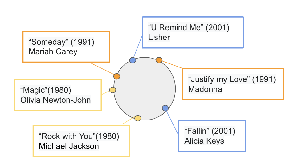
(a) without EC loss.

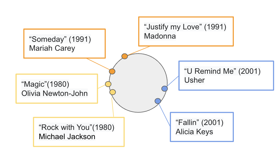
(b) with EC loss.

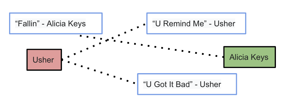
(c) without MMC loss.

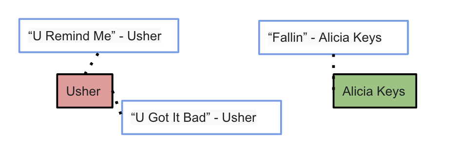
(d) with MMC loss.

Fig. 1: Illustrating the effects of contrastive learning. From (a) to (b), EC loss help aggregating songs based on the era classes. From (c) to (d), MMC loss improves clustering songs based on artists.

2.2 Supervised Contrastive (SUC) Learning

Despite the large scale CNNs can be a powerful model, we consider its architecture and training scheme using cross-entropy loss are still insufficient to tackle the discrimination of nearby eras. Therefore, we develop a novel architecture, called Audio-SUC, to incorporate the contrastive learning [8, 19, 20, 21, 22], which aims to learn robust representations by discriminating positive and negative embedding pairs based on the era labels.

Specifically, we follow [8] to design the era contrastive (EC) loss, which forces clusters of audio embedding belonging to the same era class to be pulled together in the embedding space, and meanwhile pushes apart the audio embeddings from different era classes. To this end, an learnable projection head is defined as $g_{{\bm{\theta}}}:\{{\bm{h}}_{a}\}\rightarrow{\bm{z}}$, where ${\bm{h}}_{a}$ is the encoded embedding from mel-spectrogram $\operatorname{\mathbf{x}}$, and ${\bm{z}}$ is the latent representation.

For training, we first organize the training songs by their era labels. Let $I$ be the training set, ${\bm{z}}_{i}$ be the latent representation for song $i$, and $P(i)$ be the set with the same era label as song $i$’s, while $N(i)$ be the set with different labels from song $i$’s. The learning process is illustrated in Fig. 1(a) and Fig. 1(b). Then, the EC loss can be defined as follows:

$$\mathcal{L}_{EC}=-\sum_{i\in I}\sum_{j\in P(i)}\text{log}\frac{\sigma({\bm{z}}_{i}\cdot{\bm{z}}_{j}/\tau)}{\sum_{k\in N(i)}\sigma({\bm{z}}_{i},{\bm{z}}_{k}/\tau)},$$ (3)

where $\sigma(\cdot)$ is the non-linear transform which adopts an exponential function, and $\tau$ is the temperature parameter. Note that $\mathcal{L}_{EC}$ brings two beneficial properties [8]: $(\textup{\it i})$ ability to align all available positive samples; $(\textup{\it ii})$ ability to mine hard positive and negative pairs. These properties can lead to a more robust representation of learning in our supervised scenario.

2.3 Multi-Modal Contrastive (MMC) Learning

Fig. 2 presents the era distribution of an In-House dataset across years, indicating a high imbalance between pre- and post-2000. In this ection, we propose the Multi-Modal Contrastive Learning to tackle this issue.

2.3.1 Multi-Modal Fusion Module

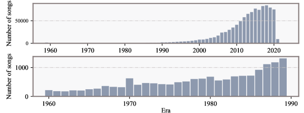
Fig. 2: Era distribution of our In-House dataset. Upper sub-figure covers the years of from 1960 to 2020. Lower sub-figure enlarges the years of pre-1990.

Multi-modal approaches have increasingly attracted researchers’ attention owing to their promising results on various deep learning tasks [23, 24]. To learn a better music representation, text about the music, such as lyrics, can be helpful augmented information and has been widely used in MIR tasks [25, 26, 27]. However, given a song, its lyrics are not always available for reasons such as copyright issues. Alternatively, the text of the artist’s biography contains rich information about the music style during the artist’s active years [28]. We choose the artist’s biography considering its availability as opposed to lyrics.

We follow the previous work [29] to make full use of contextual and correspondence information between music and text via attention mechanism, as illustrated in Fig. 3(a). Given an input song $i$, we use two embedding vectors, $\operatorname{\mathbf{a}}_{i}\in\mathbb{R}^{d_{h}}$ and $\operatorname{\mathbf{t}}_{i}\in\mathbb{R}^{d_{h}}$, to represent its audio and artist biography information, respectively, and $d_{h}=64$ is adopted in the experiments. Specifically, $\operatorname{\mathbf{a}}_{i}$ is derived from the mel-spectrogram $\operatorname{\mathbf{x}}_{i}$ using the audio encoder. For $\operatorname{\mathbf{t}}_{i}$, we utilize Sentences-BERT [30] to encode the corresponding artist biography text. Then, we concatenate $\operatorname{\mathbf{a}}_{i}$ and $\operatorname{\mathbf{t}}_{i}$ to obtain ${\bm{s}}_{i}\in\mathbb{R}^{2d_{h}}$ as the input of the self-attention layer.

The fusion module is based on Transformer blocks [31]. Specifically, the output of $l$-th Transformer block $\mathbf{\tilde{H}}_{\ell}$ is the concatenation of multiple attention heads: $\mathbf{\tilde{H}}_{\ell}=[\mathbf{A}_{{\ell},\text{1}},\cdots,\mathbf{A}_{\ell,h}]$ where $h$ is the number of heads. Each head $\bf A$ contains trainable parameters $\mathbf{W^{Q}}_{\ell},\mathbf{W}^{K}_{\ell},\mathbf{W}^{V}_{\ell}\in\mathbb{R}^{2d_{h}\times d_{k}}$, where $d_{k}$ is the projection dimension of the attention layer.

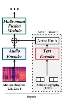
(a) Audio-Artist Encoder

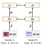
(b) Contrastive Learning Framework

Fig. 3: The overall illustration of AudioArt-MMC. (a) is the Audio-Artist Encoder mainly contains audio encoder, artist biography text encoder and a multi-modal fusion module. (b) shows the encoded latent representation ${\bm{z}}$ that goes through corresponding projection heads for MMC loss and EC loss, respectively.

2.3.2 Multi-Modal Contrastive (MMC) Loss

The EC loss $\mathcal{L}_{EC}$ conditioning on the era labels directly helps improve the era classification task. However, it may excessively blur the differences of songs in the multi-modal embedding space within the same era class. Therefore, to avoid the representation collapse, we develop the multi-modal contrastive (MMC) loss, an unsupervised contrastive learning objective. The critical part for the effectiveness of MMC learning is a reasonable design of different views of the input. For example, in computer vision, data augmentation techniques such as cropping and rotation are applied to one anchor image and the other to create positive and negative views of the anchor image. Similarly, we propose text-shuffle, a technique to create multiple views for the combination of audio and artist embeddings input. To be specific, we consider the concatenation of matched audio and artist embeddings ${\bm{s}}_{i,i}=[\operatorname{\mathbf{a}}_{i},\operatorname{\mathbf{t}}_{i}]$ as a reference, so the concatenation of mismatched audio and artist creates negative views, e.g., ${\bm{s}}_{i,k}=[\operatorname{\mathbf{a}}_{i},\operatorname{\mathbf{t}}_{k}]$, where $\operatorname{\mathbf{t}}_{k}$ is a randomly sampled biography embedding from a different artist. To apply the MMC loss, two components are designed as follows:

• Audio-Artist Encoder: $f_{E}:\{{\bm{s}}\}\rightarrow{\bm{h}}_{m}$, where ${\bm{h}}_{m}$ is the multi-modal embedding learned from the audio-artist concatenation embedding ${\bm{s}}$.

• Projection Head: $f_{T}:\{\operatorname{\mathbf{t}}\}\rightarrow{\bm{h}}_{m}$, which projects the artist biography $\operatorname{\mathbf{t}}$ into the multi-modal embedding space.

For simplicity, we take the artist biography as the anchor. Let an artist embedding $\operatorname{\mathbf{t}}_{i}$ be the anchor, its positive and negative examples in the audio-artist concatenation embedding space are ${\bm{s}}_{i,i}$ and ${\bm{s}}_{i,k}$, respectively. The MMC loss is then defined as:

$$\mathcal{L}_{MMC}=-\sum_{c\in\mathrm{C}}\sum_{i\in c(i)}\text{log}\frac{\sigma\left(f_{T}(\operatorname{\mathbf{t}}_{i})\cdot f_{E}({\bm{s}}_{i,i})/\tau\right)}{\sum_{k\in c(i)}\sigma\left(f_{T}(\operatorname{\mathbf{t}}_{i})\cdot f_{E}({\bm{s}}_{i,k})/\tau\right)},$$ (4)

where $\sigma(\cdot)$ is the exponential function, $\mathrm{C}$ is the all possible era labels, $c$ is the era label of song $i$, and $c(i)$ is the set having the era label $c$. The learning process is illustrated in Fig. 1(c) and Fig. 1(d). As illustrated in Fig. 3(b), we obtain the AudioArt-MMC model, which is trained with a sum of the cross-entropy (MLE) loss, era contrastive (EC) loss, and multi-modal contrastive (MMC) loss:

$$\mathcal{L}=\mathcal{L}_{\mathrm{MLE}}+\alpha\mathcal{L}_{MMC}+\beta\mathcal{L}_{EC},$$ (5)

where $\alpha$ and $\beta$ are hyperparameters weighting the loss terms. Note that, AudioArt-MMC uses the multi-modal embedding for $g_{\theta}$ to calculate $\mathcal{L}_{EC}$ (see Eq. 3), while Audio-SUC uses the audio embedding encoded from mel-spectrogram for $\mathcal{L}_{EC}$.

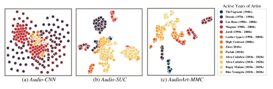
Fig. 4: The t-SNE visualization of the latent representation of different methods. The active years of an artist is marked in the parenthesis.

3 Experiments

3.1 Experiment Setup

Datasets & Metrics. To evaluate our proposed methods, we used a public dataset, Million Song Dataset (MSD) [32], and an internal music collection (In-House). MSD, which has been widely used in music auto-tagging evaluations [11], contains the metadata and pre-computed audio features of one million contemporary songs. Our In-House dataset includes about 800K songs, where the era distribution is presented in Fig. 2. For artist biography, we adopted the AllMusic dataset [33], which covers the biography text data of about 200K artists. We created the audio-text input pairs by matching the artist names. We selected 85,475 tracks from MSD for the experiments, considering the availability of audio features, release years, and artist biographies. Whereas, the full set of In-House was used, since it covers all the required information.

The difference in instrumentation and genre of songs released in close years can be subtle. Therefore, we follow similar works [34, 35] to propose a metric that allows false prediction tolerance. We define the accuracy with $\pm x$ years of tolerance (ACC_x) as follows:

$$\text{ACC}_{x}=\frac{1}{N}\sum_{i=1}^{N}\frac{x-\text{min}[\text{abs}(y_{i}-\hat{y_{i}}),x]}{x},$$ (6)

where $y_{i}$ and $\hat{y_{i}}$ represent the ground truth and predicted years of song $i$, and $N$ is the total number of test songs. For instance, ACC₀ counts only the cases when the prediction exactly matches the ground truth. We define two evaluation scenarios of granularity for year ranges: $(\textup{\it i})$ one year per class: each year represents a class. For example, songs released in 1981 are assigned with a different class than songs released in 1982. $(\textup{\it ii})$ ten years per class: each class represents a decade (e.g., 60s, 80s, and 00s). Therefore, songs released in 1981 and 1982 are within the ‘1980s’ class, while the song in 2011 is labeled with ‘2010s’ class.

Training Details. To extract the input mel-spectrograms, we first resample the original audio waveform to 22,050 Hz. Then, we use a window size of 2,048 with a hop size of 512 for a frame, and transform each frame into a 224-band mel-scaled magnitude spectrum. In the training stage, we set a batch size of 64. Each audio example, which includes 1,024 frames (roughly 6-seconds long), is randomly sampled from an arbitrary song in the training data. We use the Adam optimizer [36] with a learning rate of 1e-4.

	MSD				In-House
Method	ACC0	ACC1	ACC2	ACC3	ACC0	ACC1	ACC2	ACC3
64 classes (one year per class)
AudioArt-MMC	.238	.451	.588	.628	.188	.350	.476	.650
Audio-SUC	.213	.313	.426	.544	.140	.196	.436	.579
Audio-CNN	.138	.169	.271	.302	.097	.157	.334	.486
8 classes (ten years per class)
AudioArt-MMC	.788	.975	.988	-	.750	.978	.986	-
Audio-SUC	.675	.917	.958	-	.563	.920	.973	-
Audio-CNN	.519	.902	.964	-	.433	.865	.954	-

Table 1: Results of the one year/class and ten year/class are reported. Best results of each dataset and metric are marked bold.

3.2 Results and Discussion

We performed 10-fold cross-validation to obtain the results, and this process was done on MSD and In-House independently. We split 10% of the training set as the validation set, and selected the snapshot with best performance on validation set as the testing model.

Era Prediction Comparison. Table 1 presents the overall comparison of the two datasets. It is clear that incorporating the supervised contrastive learning (Audio-SUC) can significantly outperform the baseline model (Audio-CNN) for most of the cases (except the ACC₂ in the 8 classes scenario on MSD), and that jointing the audio and artist information for input with the multi-modal contrastive learning (i.e., AudioArt-MMC) can consistently further the performance. Such a result is in line with our expectations when designing the models. As suggested in prior work [5], artist information is very helpful in hit song prediction of a period of time, so it also offers strong clues about the musical sounds representing an era. Comparing among ACC values with different tolerances for the 64 classes scenario, the superiority of the contrastive learning-based models over CNN seems to become more apparent when the tolerance is getting larger. This indicates that the learned features indeed possess abilities for era discrimination. Lastly, for the 8 classes scenario (i.e., decade tagging), ACC₁ can achieve 90%+ accuracy solely based on audio, demonstrating promising results for a usable system in relevant MIR applications.

Robustness to Data Imbalance. As discussed, our dataset is imbalanced in era distribution. We are interested in the performance of the pre-2000 era, so we present the result of the corresponding subset in In-House. Table 2 shows the results on the pre-2000 subset and the difference $\Delta$ from their counterparts in Table 1. Note that smaller $\Delta$ is better. Comparing the $\Delta$ values among the three variants, AudioArt-MMC shows significantly smaller performance gaps between the full-set and subset results, indicating its stronger ability to handle the imbalanced data.

Visualization of Embeddings. Finally, we perform a qualitative examination of the effect of the proposed MMC loss by visualizing the embeddings of the penultimate layer from the three proposed models using t-SNE plots. We randomly select 400 songs associated with 13 artists and plot the corresponding song embeddings in the 2D space. Each artist is assigned a unique color, with brighter colors for recenter eras. As displayed in Fig. 4, EC loss can facilitate the embeddings of same era class to be closer while maintaining the diversity of different songs (see Fig. 4(b)), and MMC loss further forces aggregating songs of the same artist (see Fig. 4(c)).

Method	ACC0	ACC1	ACC2	ACC3	$\Delta_{0}$	$\Delta_{1}$	$\Delta_{2}$	$\Delta_{3}$
AudioArt-MMC	.175	.287	.393	.488	.013	.063	.083	.162
Audio-SUC	.094	.122	.237	.379	.046	.074	.097	.200
Audio-CNN	.055	.093	.162	.295	.042	.064	.172	.191

Table 2: Results for the pre-2000 subset of In-House in the 64 classes (one year/class) scenario. $\Delta_{i}$ corresponds to the ACC_i difference between the pre-2000 subset and the whole dataset.

4 Conclusion

In this paper, we have presented a novel multi-modal contrastive learning framework to recognize music era based on audio and artist information. The design of the EC and MMC losses enables a satisfactory clustering behaviors, showing convincing results for the task. For future work, we will try to improve the performance with more sophisticated solutions. We also plan to study the possibility of including additional metadata, such as instrumentation, genre, and mood, into a unified framework.

5 Acknowledgement

This work was supported by National Key R&D Program of China (2019YFC1711800) and NSFC (62171138).

References

- [1] P. Ball, The music instinct: how music works and why we can’t do without it, Random House, 2010.
- [2] D. Huron, Sweet anticipation: Music and the psychology of expectation, MIT press, 2008.
- [3] H. Honing, Musical cognition: a science of listening, Routledge, 2017.
- [4] J. Serrà, Á. Corral, M. Boguñá, M. Haro Berois, and J. L. Arcos, “Measuring the evolution of contemporary western popular music,” Scientific reports. 2012;(2): 521, 2012.
- [5] M. Interiano, K. Kazemi, L. Wang, J. Yang, Z. Yu, and N. L. Komarova, “Musical trends and predictability of success in contemporary songs in and out of the top charts,” Royal Society open science, vol. 5, no. 5, pp. 171274, 2018.
- [6] T. Pohle, P. Knees, M. Schedl, E. Pampalk, and G. Widmer, ““reinventing the wheel”: a novel approach to music player interfaces,” IEEE Transactions on Multimedia, vol. 9, no. 3, pp. 567–575, 2007.
- [7] M. Schedl, D. Hauger, and D. Schnitzer, “A model for serendipitous music retrieval,” in Proc. Workshop on Context-awareness in Retrieval and Recommendation, 2012, pp. 10–13.
- [8] P. Khosla, P. Teterwak, C. Wang, A. Sarna, Y. Tian, P. Isola, A. Maschinot, C. Liu, and D. Krishnan, “Supervised contrastive learning,” Proc. NeurIPS, vol. 33, pp. 18661–18673, 2020.
- [9] T. Chen, S. Kornblith, M. Norouzi, and G. Hinton, “A simple framework for contrastive learning of visual representations,” in Proc. ICML, 2020, pp. 1597–1607.
- [10] K. Hoashi, K. Matsumoto, and N. Inoue, “Personalization of user profiles for content-based music retrieval based on relevance feedback,” in Proc. ACM Multimedia, 2003, p. 110–119.
- [11] J. Nam, K. Choi, J. Lee, S.-Y. Chou, and Y.-H. Yang, “Deep learning for audio-based music classification and tagging: Teaching computers to distinguish rock from bach,” IEEE signal processing magazine, vol. 36, no. 1, pp. 41–51, 2018.
- [12] K. Choi, G. Fazekas, and M. Sandler, “Automatic tagging using deep convolutional neural networks,” arXiv preprint arXiv:1606.00298, 2016.
- [13] J. Pons, O. Nieto, M. Prockup, E. Schmidt, A. Ehmann, and X. Serra, “End-to-end learning for music audio tagging at scale,” arXiv preprint arXiv:1711.02520, 2017.
- [14] M. Won, S. Chun, O. Nieto, and X. Serrc, “Data-driven harmonic filters for audio representation learning,” in Proc. ICASSP, 2020, pp. 536–540.
- [15] E. Zangerle, M. Vötter, R. Huber, and Y.-H. Yang, “Hit song prediction: Leveraging low-and high-level audio features.,” in ISMIR, 2019, pp. 319–326.
- [16] L.-C. Yang, S.-Y. Chou, J.-Y. Liu, Y.-H. Yang, and Y.-A. Chen, “Revisiting the problem of audio-based hit song prediction using convolutional neural networks,” in Proc. ICASSP, 2017, pp. 621–625.
- [17] L.-C. Yu, Y.-H. Yang, Y.-N. Hung, and Y.-A. Chen, “Hit song prediction for pop music by siamese cnn with ranking loss,” arXiv preprint arXiv:1710.10814, 2017.
- [18] K. Ibrahim, E. Epure, G. Peeters, and G. Richard, “Should we consider the users in contextual music auto-tagging models?,” in Proc. ISMIR, 2020.
- [19] J. Yu, H. Yin, X. Xia, T. Chen, L. Cui, and Q. V. H. Nguyen, “Are graph augmentations necessary? simple graph contrastive learning for recommendation,” in Proc. ACM SIGIR, 2022, pp. 1294–1303.
- [20] Y. Marrakchi, O. Makansi, and T. Brox, “Fighting class imbalance with contrastive learning,” in International Conference on Medical Image Computing and Computer-Assisted Intervention. Springer, 2021, pp. 466–476.
- [21] Z. Jiang, T. Chen, B. J. Mortazavi, and Z. Wang, “Self-damaging contrastive learning,” in Proc. ICML, 2021, pp. 4927–4939.
- [22] P. Wang, K. Han, X.-S. Wei, L. Zhang, and L. Wang, “Contrastive learning based hybrid networks for long-tailed image classification,” in Proc. CVPR, 2021, pp. 943–952.
- [23] W. Ding, M. Xu, D. Huang, W. Lin, M. Dong, X. Yu, and H. Li, “Audio and face video emotion recognition in the wild using deep neural networks and small datasets,” in Proc. ACM Multimodal Interaction, 2016, pp. 506–513.
- [24] S. Pini, O. B. Ahmed, M. Cornia, L. Baraldi, R. Cucchiara, and B. Huet, “Modeling multimodal cues in a deep learning-based framework for emotion recognition in the wild,” in Proc. ACM Multimodal Interaction, 2017, pp. 536–543.
- [25] P. Lamere, “Social tagging and music information retrieval,” Journal of new music research, vol. 37, no. 2, pp. 101–114, 2008.
- [26] S. Oramas, O. Nieto, F. Barbieri, and X. Serra, “Multi-label music genre classification from audio, text, and images using deep features,” arXiv preprint arXiv:1707.04916, 2017.
- [27] S. Oramas, F. Barbieri, O. Nieto Caballero, and X. Serra, “Multimodal deep learning for music genre classification,” Trans. ISMIR, vol. 1, no. 1, pp. 4–21, 2018.
- [28] T. Li and M. Ogihara, “Music artist style identification by semi-supervised learning from both lyrics and content,” in Proc. ACM Multimedia, 2004, pp. 364–367.
- [29] F. Simonetta, S. Ntalampiras, and F. Avanzini, “Multimodal music information processing and retrieval: Survey and future challenges,” in International Workshop on Multilayer Music Representation and Processing, 2019, pp. 10–18.
- [30] N. Reimers and I. Gurevych, “Sentence-bert: Sentence embeddings using siamese bert-networks,” arXiv preprint arXiv:1908.10084, 2019.
- [31] A. Vaswani, N. Shazeer, N. Parmar, J. Uszkoreit, L. Jones, A. N. Gomez, Ł. Kaiser, and I. Polosukhin, “Attention is all you need,” Proc. NeurIPS, vol. 30, 2017.
- [32] T. Bertin-Mahieux, D. P. Ellis, B. Whitman, and P. Lamere, “The million song dataset,” in Proc. ISMIR, 2011.
- [33] R. Malheiro, R. Panda, P. Gomes, and R. P. Paiva, “Emotionally-relevant features for classification and regression of music lyrics,” IEEE Transactions on Affective Computing, vol. 9, no. 2, pp. 240–254, 2016.
- [34] R. Angulu, J. R. Tapamo, and A. O. Adewumi, “Age estimation via face images: a survey,” EURASIP Journal on Image and Video Processing, vol. 2018, no. 1, pp. 1–35, 2018.
- [35] A. Saraf and E. Khoury, “Distribution learning for age estimation from speech,” in Proc. ICASSP, 2022, pp. 8552–8556.
- [36] D. P. Kingma and J. Ba, “Adam: A method for stochastic optimization,” arXiv preprint arXiv:1412.6980, 2014.