An activity transition in FRB 20201124A:
methodological rigor,
detection of frequency-dependent cessation,
and a geometric magnetar model.
We report detections of fast radio bursts (FRBs) from the repeating source FRB 20201124A with Apertif/WSRT and GMRT, and measurements of basic burst properties, especially the dispersion measure (DM) and fluence. Based on comparisons of these properties with previously published larger samples, we argue that the excess DM reported earlier for pulses with integrated signal to noise ratio is due to incompletely accounting for the so-called sad trombone effect, even when using structure-maximizing DM algorithms. Our investigations of fluence distributions next lead us to advise against formal power-law fitting, especially dissuading the use of the least-square method, and we demonstrate the large biases involved. A maximum likelihood estimator (MLE) provides a much more accurate estimate of the power law and we provide accessible code for direct inclusion in future research. Our GMRT observations were fortuitously scheduled around the end of the activity cycle as recorded by FAST. We detected several bursts (one of them very strong) at 400/600 MHz, a few hours after sensitive FAST non-detections already showed the 1.3 GHz FRB emission to have ceased. After FRB 20180916B, this is a second example of a frequency-dependent activity window identified in a repeating FRB source. Since numerous efforts have so-far failed to determine a spin period for FRB 20201124A, we conjecture it to be an ultra-long period magnetar, with a period on the scale of months, and with a very wide, highly irregular duty cycle. Assuming the emission comes from closed field lines, we use radius-to-frequency mapping and polarization information from other studies to constrain the magnetospheric geometry and location of the emission region. Our initial findings are consistent with a possible connection between FRBs and crustal motion events.
Key Words.:
fast radio bursts – high energy astrophysics – neutron stars1 Introduction
Fast radio bursts (FRBs) are micro-to-millisecond-long bursts of radio emission of extragalactic origin (see Petroff et al., 2019, 2022, for review). Over the almost two decades since the discovery of the first FRB (Lorimer et al., 2007), multiple FRB emission theories have been proposed (for the live catalogue see Platts et al., 2019). So far no consensus about their exact origin has emerged, although neutron star progenitors currently appear favored.
It is even possible that several classes of progenitors emit FRBs. At the moment, the most obvious empirical demarcation between these types is the dichotomy between one-off sources and FRB repeaters. Only the former are potentially cataclysmic. These two classes show statistical differences in the spectro-temporal properties of the bursts (Pleunis et al., 2021a). In comparison to one-off sources, repeaters offer much more information about their circum-burst environment and the burst emission mechanism: they can be localized with much better precision and the pulses provide dynamical estimates of the electron content and magnetic field in the vicinity of the emitting plasma. Any emission theory must explain the entire distribution of burst fluences, and the various spectro-morphological properties of pulses that originate in the same local environment.
While some FRBs are only seen to repeat a handful of times, FRB 20201124A is a veritable FRB factory: it is capable of emitting prolifically, and datasets covering it contain hundreds of pulses. It is thought to be located in a dynamically evolving magnetized environment, as suggested by irregular rotation measure (RM) variations on short timescales and the presence of Faraday conversion (Xu et al., 2022). FRB 20201124A is notorious for its high but exceedingly variable pulse emission rate. The source was first detected at the end of 2020 by the Canadian Hydrogen Intensity Mapping Experiment (CHIME), but only after about 40 hrs of earlier observations of the same field contained no detections (Lanman et al., 2022). By 2021 March-May FRB 20201124A had entered a high-activity phase, the “Spring 2021” or “S21” epoch hereafter111Given the source declination of we label the activity spans by the northern hemisphere seasons., reaching rates almost 50 bursts per hour, as observed by the Five-hundred-meter Aperture Spherical radio Telescope (FAST) at 20 cm wavelength (Xu et al., 2022). The S21 FAST burst sample was complemented by observations performed with CHIME, the Effelsberg 100-m and the Parkes 64-m dishes, the upgraded Giant Metrewave Radio Telescope (uGRMT), and ASKAP, the Australian Square Kilometre Array Pathfinder (Lanman et al., 2022; Hilmarsson et al., 2021; Marthi et al., 2022; Kumar et al., 2022).
Bursts from FRB 20201124A exhibit a high degree of circular and linear polarizations, with predominantly flat position angle (PA) curves. These polarization properties hint at a magnetospheric origin (Jiang et al., 2022). Such an origin a grees with a rotating neutron-star progenitor hypothesis. However, despite extensive searches, no periodicity has been found in the high number of bursts, over a broad range of trial periods spanning milliseconds to days (Niu et al., 2022; Du et al., 2023).
The FAST observations indicate that the S21 activity epoch ended abruptly between 2021 May 26 and 29 (Xu et al., 2022, observations at 1250 MHz). On May 27 CHIME/FRB recorded one more burst from this FRB at the lower frequencies of 400–800 MHz (Lanman et al., 2022), followed by a bright burst at 1350 MHz detected by the Stockert telescope on May 28, during a 3-day gap in FAST coverage (Kirsten et al., 2024) . The gaps in the observing schedules of these three telescopes did not allow further constraints on any possible frequency-dependent boundaries of the activity phase, an effect seen in one other repeating FRB, FRB 20180916B (Pastor-Marazuela et al., 2021). The end of the activity cycle was, however, also covered by GMRT observations at 300–750 MHz. Strikingly, GMRT detected several low-frequency pulses on June 1, several hours after the FAST non-detections showed the higher-frequency bursts had already turned off.
Despite continued monitoring (Mao et al., 2022; Trudu et al., 2022), these June 1 pulses were the only signs of activity detected from FRB 20201124A until the pulses reappeared at some time before 2021 September 21 (Main et al., 2021, also CHIME222https://www.chime-frb.ca/repeaters/FRB20201124A). An extensive FAST monitoring campaign then observed an exponentially increasing FRB rate, reaching activity levels an order of magnitude higher than those Xu et al. reported earlier. The activity in this “Fall 2021” (F21) epoch abruptly quenched again between September 28 and 29 (Zhou et al., 2022). No detections are next published until late 2022 January (the “Winter 2022”, W22 epoch; Ould-Boukattine et al., 2022).
The repeater field was regularly scheduled in the Apertif-LOFAR333The APERture Tile In Focus and LOw-Frequency ARray, respectively. Exploration of the Radio Transient sky (ALERT) survey, that started in 2019 at the Westerbork Synthesis Radio Telescope (WSRT; Maan & van Leeuwen, 2017; van Leeuwen et al., 2023; Pastor-Marazuela et al., 2024). During the last observing run of this survey, in the first week of 2022 February, the three observing sessions towards FRB 20201124A yielded ten FRB detections.
This work describes the properties of those bursts detected within the ALERT survey in W22, as well as of GMRT bursts from the S21 and W22 activity cycles. We include the analysis of dispersion measures (DMs), fluence distributions, (quasi-)periodicities, and scintillation of these bursts.
The evidence we find for a frequency-dependent activity cycle, together with the energetics and morphological properties of the recorded pulses – both in our sample and in the large FAST sample – provide an unique test of the hypothesis that FRBs originate from low-twist ultra-long period (ULP) magnetars (Wadiasingh & Timokhin, 2019; Wadiasingh et al., 2020; Beniamini et al., 2020; Caleb et al., 2022). That is interesting, because a variety of scenarios have been proposed on how neutron stars might form FRBs, but testing and distinguishing these observationally is challenging.
In the ULP hypothesis, FRBs are generated via a pulsar-like emission mechanism in the magnetospheres of very slowly rotating magnetars. In these sources, the non-potential magnetosphere (i.e., one in which currents flow) is characterized by an unusually weak large-scale magnetic field twist, much weaker than that of ”normal” galactic magnetars. This results in a low plasma density on the closed magnetic field lines. In such charge-starved conditions, deformations in the crust that dislocate the footpoints of the magnetic field lines generate strong transient electric fields. This, in turn, leads to avalanche pair production and, ultimately, the emission of FRBs via a pulsar-like, coherent mechanism.
The low-twist magnetar hypothesis of FRB generation makes specific predictions for the times of arrival (TOAs) of individual bursts, and for the quasi-periodicity of sub-bursts. In this work, we compare these predictions to existing observational evidence. Finally, we put constraints on the location and shape of active regions on the surface of the star, by using two classical phenomenological models of radio pulsar emission: radius-to-frequency mapping and rotating vector models.
2 GMRT observations and analysis
| Burst # | (MHz) | Topo TOA (MJD) | DM (pc cm-3) | Equiv. width (ms) | Peak Flux (Jy) | (Jy ms) |
|---|---|---|---|---|---|---|
| G01 | 400 | 59366.29432631 | 412.7 | 42 | 3.8 | 160 |
| G02 | 400 | 59366.31507238 | 412.5 | 19 | 2.1 | 40 |
| G03 | 650 | 59366.30413889 | 414.5 | 15 | 3.2 | 48 |
| G04 | 650 | 59366.31848719 | 416.0 | 18 | 4.1 | 72 |
| G05 | 650 | 59366.32968037 | 415.5 | 16 | 43.4 | 679 |
| G06 | 650 | 59366.34033776 | 415.0 | 33 | 4.4 | 144 |
| G07 | 650 | 59616.77764372 | 419.8 | 23 | 2.2 | 51 |
| G08 | 650 | 59617.55751631 | 417.2 | 11 | 2.6 | 28 |
| G09 | 650 | 59617.56061649 | 412.2 | 18 | 1.2 | 22 |
| G10 | 650 | 59617.56817339 | 416.4 | 13 | 2.1 | 27 |
| G11 | 650 | 59617.57193117 | 421.0 | 29 | 2.1 | 59 |
| G12 | 650 | 59617.59070828 | 416.0 | 20 | 1.8 | 34 |
| G13 | 650 | 59617.55159768 | 418.2 | 18 | 1.4 | 26 |
| G14 | 650 | 59617.55230447 | 421.0 | 20 | 1.4 | 28 |
| G15 | 650 | 59617.63759893 | 413.4 | 7 | 1.5 | 11 |
| G16 | 650 | 59617.61070096 | 413.6 | 12 | 2.3 | 26 |
2.1 Observations
We observed FRB 20201124A with the uGMRT (Gupta et al., 2017) on 2021 June 01, July 03 & 04, and 2022 February 05, 06 & 07, under Director’s Discretionary Time. Except for one session, FRB 20201124A was observed simultaneously in the band 3 (300–500 MHz) and band 4 (550–750 MHz) of GMRT, by combining the antennae in two different sub-arrays. These dual-band observations thus provided a frequency coverage of 300–750 MHz. The observing setup utilized the phased-array beam (PAB) sensitivity of typically 11 antennae in each of the two sub-arrays. At band 4, data were recorded at 4096 channels across 200 MHz bandwidth centered at 650 MHz, with a sampling time of 0.328 ms. At band 3, the data were coherently dedispersed in real-time at a DM of 410.9 pc cm-3, and then recorded to disk with 1024 sub-bands across 200 MHz bandwidth centered at 400 MHz, using a sampling time of 0.164 ms. The last session on 2022 February 07 was conducted only in band 4 utilizing a higher sensitivity obtained by combining 16 antennae in a single sub-array, and the PAB data were coherently dedispersed at a DM of 410.9 pc cm-3 in real-time and then recorded to the disk with 1024 sub-bands and a sampling time of 40.96 s. During all the observations conducted in 2022, data from the incoherent-array beam (IAB) formed using the same antennae in the individual sub-arrays were also recorded simultaneously with the PAB. The availability of the IAB data facilitate a better excision of the radio frequency interference (RFI).
2.2 Preprocessing and search for radio bursts
The individual band data from all the sessions were processed through the following series of data reduction steps. For the band 4 observations, which did not employ the real-time coherent dedispersion, we used SIGPROC’s dedisperse to create 1024 sub-bands, by dedispersing sets of 4 channels to a single subband, using a DM of 410.9 pc cm-3. As mentioned above, all the band 3 observations were already recorded with 1024 coherently dedispersed sub-bands (the real-time coherent dedispersion removes only the intra-sub-band smearing). The individual band data from each of the sessions were then subjected to down-sampling from 16 bits to 8 bits per sample using digifil, and RFI excision using RFIClean444https://github.com/ymaan4/RFIClean (Maan et al., 2021) and rfifind from the pulsar search and analysis toolkit PRESTO (Ransom et al., 2002).
For the observations conducted in 2022, we formed the post-correlation beam (Roy et al., 2018) using the PABs and IABs (i.e., we subtracted the IAB from the PAB after appropriate scaling555https://github.com/ymaan4/pcBeam-GMRT). This post-correlation beam contains less red noise, mitigates some RFI and thus reduces false candidates while searching for bright pulses. This beam was processed through the same steps described above.
The sub-banded data were then incoherently dedispersed in steps of 0.05 and 0.2 pc cm-3, covering the DM range 400–425 pc cm-3 in 500 and 125 trial DMs, for band 3 and band 4 respectively, using prepdata from PRESTO. The above configurations limit the dispersive smearing to a maximum of 1 ms throughout the explored DM range for both bands. Each dedispersed time-series was searched for the presence of bright pulses above a signal-to-noise ratio (S/N) threshold of 8 and a maximum pulse-width of 50 ms using single_pulse_search.py. All the single pulse candidates were next grouped by looking for the brightest candidates within roughly 100 or 200 ms wide time windows and across all the trial DMs. Waterfall plots for all the grouped candidates were scrutinized by eye to identify the genuine bursts.
Each dedispersed time-series was also searched for periodic signals using accelsearch from PRESTO, with zmax set to 256. For each observation, all the periodic signal candidates were sifted for harmonics and duplicates at different DM trials, and the final candidates were folded using prepfold and the diagnostic plots were examined by human experts.
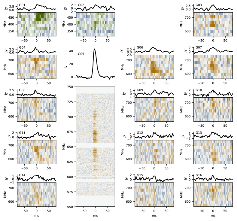
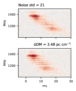
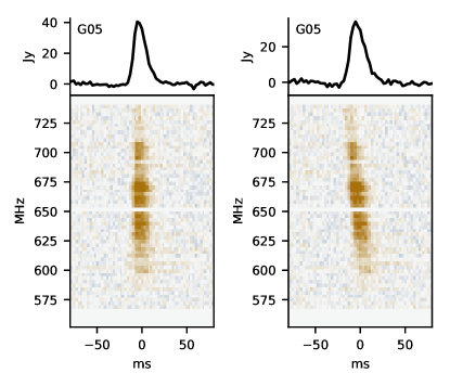
Overall, 16 bursts were detected, six during the 2021 June 01 session, one on 2022 February 6 and the rest on February 07. The bursts are labeled G01–G16 following their TOA order. Figure 1 shows spectra and band-integrated profiles for the obtained burst sample, whereas Table 1 lists their properties.
All bursts except G05 are faint and little more can be inferred from their spectro-temporal shapes than a hint of downward-drifting trombone features, when dedispersed to the DM obtained from G05 (see Section 4.1). Overall, the peak flux densities, fluences and equivalent widths are comparable to the FRB 20201124A bursts recorded earlier with GMRT, in 2021 April (Marthi et al., 2022).
3 ALERT observations and analysis
Apertif is a phased-array front-end system installed on 12 of the 14 WSRT dishes666Westerbork dish RT1 also monitors FRBs, in stand-alone mode (e.g., Kirsten et al. 2024). We hereafter call that mode Wb-RT1. All other references to WSRT imply Apertif. (Adams & van Leeuwen, 2019; van Cappellen et al., 2022). Apertif observed FRB 20201124A as part of the scheduled visits of repeater fields in the ALERT survey (Oostrum et al., 2020; van Leeuwen et al., 2023), on 2021 July 03 & 04, and on 2022 February 01, 05, & 06. The last two observations were coordinated to overlap with GMRT (see Sect. 3.2). All sessions lasted for three hours except for a 2.4-hr-long session on February 05.
Apertif consists of phase array feeds on a multi-element interferometer, that form a hierarchical system of beams. During the FRB 20201124A observations, the central compound beam CB00 was pointed at the J2000 sky coordinates , ( for July 2021 sessions). These coordinates are close to the source position at , as reported by Nimmo et al. (2022). The offset lies well within the Apertif localization limits (Oostrum, 2020).
Total intensity samples were recorded at a time resolution of 81.92 s, and with 1536 channels of 195.312 kHz for a sample bandwidth of 300 MHz centered at 1369.6 MHz. As part of the standard real-time FRB search, the data from all 40 compound beams was independently searched for FRBs, using the AMBER777https://github.com/TRASAL/AMBER search code (the Apertif Monitor for Bursts Encountered in Real-Time; Sclocco et al., 2016) in the DARC888https://github.com/loostrum/darc pipeline (the Data Analysis of Real-time Candidates; Oostrum, 2021) on the Apertif Radio Transient System (ARTS; van Leeuwen, 2014). Real-time candidate selection was carried out by a neural network, as described in Connor & van Leeuwen (2018).
The DARC pipeline did not find any candidates in the July sessions. This is in line with the reports by Main et al. (2021) on targeted observations with both uGMRT and the Effelsberg Telescope over 2021 June–Aug. Mao et al. (2022) also did not find any bursts down to 4 Jy ms during a 104-hr observing run with Nanshan 26-m Radio Telescope in 2021 June-July.
During the 2022 February ALERT run, two bright FRBs were detected on the 1st, at pc cm-3. Initially, the bursts were found in CB17, which partially overlaps CB00 (Fig. 3 in van Leeuwen et al., 2023). Fluences and dispersion measures for these bursts were previously reported in Atri et al. (2022). Subsequent reanalysis showed the pulses were not detected in CB00 because of the residual RFI. The next session, on the February 05, yielded one more burst. No bursts were detected on the February 06, despite comparable system parameters and RFI.
3.1 Deep search
We subsequently performed an offline search over a finer grid of trial DMs and matched-filter boxcar widths than is possible in the real-time search. First, the filterbank files from CB00 were thoroughly cleaned of RFI using the iqrm999https://gitlab.com/kmrajwade/iqrm_apollo software implementation of the Inter-Quartile Range Mitigation outlier detection algorithm (Morello et al., 2022) and using rficlean101010https://github.com/ymaan4/RFIClean, which operates in the Fourier domain (Maan et al., 2021).
Pulse candidates were selected using TransientX111111https://github.com/ypmen/TransientX (Men & Barr, 2024). We searched for FRBs over DMs ranging from 360 to 460 pc cm-3 with a step of 0.25 pc cm-3. Boxcar filter widths ranged from 0.18 ms (slightly over two samples) to 200 ms. Each session yielded about 500 potential FRBs with integrated , which were inspected visually. Most of the candidates were residual RFI, displaying sharp, narrow-band positive and negative jumps in the frequency-resolved signal. Only 24 pulses possessed the FRB-like properties we defined, being relatively broadband and displaying smooth variation of signal strength with frequency. Three brighter candidates matched earlier DARC detections.
| Burst # | TOA (MJD) | DM (pc cm-3) | S/N | Width (ms) |
|---|---|---|---|---|
| 59398.32763124 | 432.50 | 7.1 | 4.1 | |
| 59398.35390255 | 423.00 | 7.3 | 3.4 | |
| 59399.30523345 | 407.50 | 7.5 | 0.7 | |
| 59399.33769469 | 377.00 | 7.3 | 1.1 | |
| 59611.83116861 | 424.00 | 7.1 | 21.3 | |
| W01 | 59611.83130447 | 418.50 | 93.3 | 3.4 |
| 59611.83210172 | 369.50 | 7.7 | 0.6 | |
| W02 | 59611.84358984 | 434.00 | 10.5 | 11.4 |
| 59611.84811625 | 416.75 | 7.1 | 11.4 | |
| W03 | 59611.86041082 | 422.75 | 12.2 | 32.4 |
| W04 | 59611.87300625 | 425.75 | 11.6 | 9.3 |
| W05 | 59611.87448743 | 433.50 | 15.8 | 17.3 |
| W06 | 59611.89157873 | 428.25 | 9.1 | 9.3 |
| 59611.90475537 | 433.00 | 7.5 | 21.3 | |
| 59611.90700670 | 418.00 | 7.7 | 14.0 | |
| W07a | 59611.90761850 | 412.75 | 9.6 | 6.1 |
| W07b | 59611.90761951 | 425.50 | 57.3 | 21.3 |
| 59611.91905550 | 390.50 | 7.3 | 7.5 | |
| W08 | 59611.92021812 | 422.00 | 9.3 | 7.5 |
| W09 | 59611.92725919 | 425.25 | 11.3 | 11.4 |
| 59611.92842737 | 414.25 | 7.4 | 3.4 | |
| W10 | 59615.74587387 | 415.25 | 51.7 | 6.1 |
| 59616.73514411 | 432.00 | 7.6 | 17.3 | |
| 59616.78902312 | 424.75 | 7.4 | 9.3 |
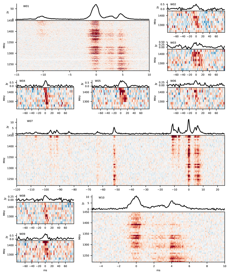
Table 2 lists the times of arrival, best DM, integrated S/N and boxcar filter width for all 24 candidates. The majority (83%) have DMs larger than 411 pc cm-3, the DM of the brightest pulses from FRB 20201124A. However, transientX optimizes DM to maximize the S/N ratio and for some bright pulses this clearly compromises the intrinsic spectro-temporal structure.
About 70% of all candidates come from one observing session, 2022 February 01. The 2021 July sessions and session 2022 February 06 yield two candidates each, and session 2022 February 05 resulted in only one (relatively bright) burst. It is possible that some of our faint candidates are due to chance noise fluctuations. In order to estimate the rate of occurrence of such noise candidates, we performed the same search in DM range between 660 and 760 pc cm-3, leaving all other parameters intact. In this manner three candidates were visually filtered from about 500 candidates per session. Two candidates were detected in session 2021 July 04 and one in 2022 February 05, their integrated S/N values were , widths ranged from 0.3 to 6.3 ms, and on the diagnostic plots the spectra looked indistinguishable from the spectra of faint FRB candidates from Table 2.
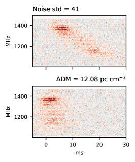
Table 2 lists 13 pulses with , significantly more than the 3 that would have been expected by chance detections following the test described above. This likely means that some of those candidates were emitted by FRB 20201124A, although we cannot tell which ones exactly. Their faintness precludes any meaningful analysis, thus we do not further include them in the sample. The spectra of the remaining ten bursts were next computed using dspsr and are shown in Fig. 2.
Calibration of the ALERT FRBs is performed with the help of drift scan observations of the bright quasars 3C147, 3C286, and 3C48 at the beginning and the end of each observing run (cf. Connor et al., 2020; Pastor-Marazuela et al., 2023). We used the calibrator observation closest to a given FRB 20201124A session and estimated the System Equivalent Flux Density (SEFD) using the known quasar flux (Perley & Butler, 2017). For 2022 February 01, the SEFD was 94 Jy and for the last two sessions it was 82 Jy. There is a slight (10%) variation within the band which was ignored. However, we took into account the excised parts of the band. Scaling the SEFD according to the radiometer equation resulted in about 170 or 200 times smaller SEFD for the band-integrated signal at the original time resolution (the denominator in Eq. A1.16 of Lorimer & Kramer 2005), depending on the number of excised channels. Following Pastor-Marazuela et al. (2021) we assume 20% errors on the flux density values.
The quasar driftscan observations in the end of the 2022 June-July observing run failed, but test observations of pulsars immediately before and after FRB 20201124A observations did not indicate any malfunction. Taking a typical SEFD of 85 Jy as derived in van Leeuwen et al. (2023), the fluence of the faint (i.e., below the adopted S/N threshold) bursts from Table 2 ranges from 0.7 to 4 Jy ms, which is comparable to the limits by Mao et al. (2022) and larger than the 0.02 Jy ms limits for 5-ms pulses after the emission quenching as reported by Xu et al. (2022). Still, we believe that the small excess of burst candidates detected near the plausible source DM (four around 410 pc cm-3 versus one candidate around the incorrect DM of 610 pc cm-3) does not provide compelling evidence for the detection of faint FRBs between S21 and F21 activity cycles. More robust estimates of the chance probabilities of such detection are beyond the scope of this work.
Among the ALERT bursts, W07 stands out because of its complex structure, appearing to consist of two groups of pulses with separations comparable to the duration of the groups themselves, clearly visible in Fig. 2. The burst was actually detected as two separate events by transientX, but in what follows we will analyze it as one cluster-burst, following the convention of Zhou et al. (2022), who, based on the waiting time distribution of the emission peaks from Xu et al. (2022), define such a “cluster-burst” as a collection of emission peaks with a separation less than 400 ms, without signs of bridge emission between them.
The ALERT rate of 3 bursts per hour is seemingly smaller than the 5.6–45.8 hr-1 reported by Xu et al. (2022). However, taking into account only those FAST pulses which satisfy the width-dependent fluence threshold based on an integrated ALERT S/N of 8.1, Jy ms, we find that the FAST rate was close to the ALERT values in the beginning of the FAST observing campaign and extrapolates to 10–14 bursts per hour for the FAST sensitivity limits.
On 2022 February 01, no pulses other than W07 appear clustered. Session 2022 February 05 yielded only one relatively bright burst, 11 minutes into the observation, but no other bursts, even faint ones, were detected later. Xu et al. (2022) report at least one instance of a change in rate by a factor 3 (5 on their full sample) between daily sessions. The absence of emission after 2022 February 5 is unlikely to be the end of this activity cycle, since Takefuji et al. (2022) observed a burst at 2.3 GHz on 2022 February 18. After that no other detections were reported.
3.2 Simultaneous observations by GMRT and ALERT
Apertif and the GMRT were co-pointing on 2021 February 05 from 18:20–19:30 UT, and on February 06 from 16:30–19:30 UT. During this time there is one burst detection, G07 (Table 1). There is no evidence for this same burst in the Apertif data. We conclude the burst emission is band limited, and does not extend from 650 MHz up to 1.4 GHz, similar to the behavior we have found earlier in FRB 20180916B (Pastor-Marazuela et al., 2021).
4 Burst analysis
| Burst # | DM (pc cm-3) | Equiv. width (ms) | Span (ms) | Peak Flux (Jy) | Fluence (Jy ms) |
|---|---|---|---|---|---|
| W01 | 410.06(13) | 3 | 15 | 69.6 | 215.3 |
| W02 | 10 | 0.5 | 5.1 | ||
| W03 | 15 | 0.5 | 7.7 | ||
| W04 | 9 | 0.7 | 6.2 | ||
| W05 | 15 | 0.8 | 12.2 | ||
| W06 | 18 | 0.4 | 7.2 | ||
| W07 | 410.01(34) | 7 | 112 | 12.6 | 98.6 |
| W08 | 14 | 0.3 | 4.2 | ||
| W09 | 15 | 0.7 | 10.9 | ||
| W10 | 409.89(42) | 3 | 5 | 10.8 | 28.5 |
4.1 Dispersion measure
Dispersion is an important characteristic of FRBs as it measures the integrated electron density on the line of sight – provided that the effect of dispersion can be separated from any intrinsic spectral shape of the burst. Variations of the DM may indicate a complex and dynamic circum-burst environment, since rapid DM changes are not expected at the galactic and inter-galactic level. When combined with the RM, the DM places limits on the magnetic field strengths encountered by the bursts (e.g. Xu et al., 2022; Lu et al., 2023).
As a quantity, the DM characterizes the magnitude of the pulse delay – a delay that is inversely dependent on the square of the observing frequency. In the absence of any a priori knowledge about the intrinsic spectral shape of a burst, the DM can be estimated by maximizing the coherent power in the burst, across the observing bandwidth (Seymour et al., 2019). This technique is employed by DM_phase121212https://www.github.com/DanieleMichilli/DM_phase which operates as follows. During dedispersion, the time series from each particular frequency channel is shifted to counteract the expected dispersive delay for this frequency. For a Fourier transform along the time axis, this operation corresponds to a multiplication by , with , where signifies the Fourier frequency. The phase of the Fourier transform is integrated over and , and the resulting dependence of integrated coherent power on the trial DM values is examined for peaks. The error of the DM measurement is assumed to be the error of peak position determination.
We have utilized DM_phase with an automatic cutoff along the axis to measure the DM for all our bursts that have an integrated . The GMRT sample yielded one such burst, with a single component and slightly asymmetrical pulse shape. For this burst, the DM was measured to be pc cm-3.
The WSRT sample contained three sufficiently bright bursts, all composed of a few distinct components. The DM measured here was lower, 410 pc cm-3, with a characteristic error of 0.3 pc cm-3 (Table 3). The initially reported measurement of pc cm-3 for bursts W01 and W07b (Atri et al., 2022) was based on the less precise method of straightening the pulse structures visually. Both the GMRT and WSRT measurements agree with the distribution of DMs within the respective activity cycles (Xu et al., 2022; Kirsten et al., 2024).
The structure-maximizing method of DM estimation is a de-facto standard in the FRB field at the moment. However, it does not provide unambiguous measurements for all bursts. For some FRBs, optimal DMs determined from the upper/lower halves of the observing band are inconsistent with each other, and burst spectral features can not be aligned across the whole band (see, e.g., Platts et al., 2021; Kumar et al., 2022; Zhou et al., 2022).
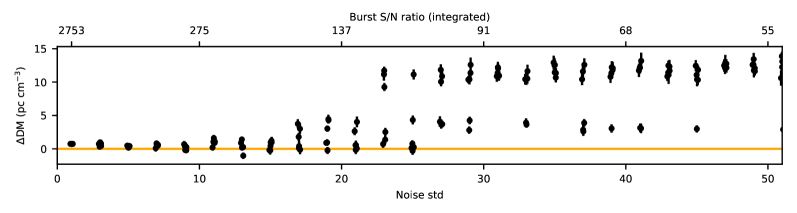
Below we will demonstrate that the existence of a DM value that maximizes burst coherent structure does not mean that this DM can be readily used to measure the integrated electron density along the path the emission traveled. Depending on the burst spectral shape, the structure-maximizing DM may be biased by fine structure buried in noise. We illustrate this using the comprehensive study of FRB 20201124A bursts by Xu et al. (2022). The authors compiled a set of DM values measured with DM_phase for bursts with integrated S/N ratio of 20–3000 and a variety of time-frequency profiles. The authors rule out secular DM trends on the level of 2.9 pc cm-3 per two months, but record a large spread of DMs (with variations of order of few pc cm-3) within individual 2-hr sessions, sometimes on a timescale of less than a minute or, remarkably, even less than a second.
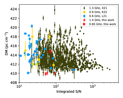
There is a correspondence between the reported DMs and the integrated S/Ns of the bursts in the Xu et al. dataset: the DMs of the brightest bursts are listed as lower (around 411 pc cm-3), whereas the reported DMs of fainter bursts are spread between 409 and 424 pc cm-3 (Fig. 3). Kumar et al. (2022) and Lanman et al. (2022) report a similar spread of DM values for comparable S/Ns131313 While Kumar et al. (2022) uses DM_phase, Lanman et al. (2022) use fitburst, which models bursts as a collection of Gaussian components with frequency-dependent amplitudes convolved with a scattering function (see CHIME/FRB Collaboration et al. 2021, for a discussion on the limitations of this approach)..
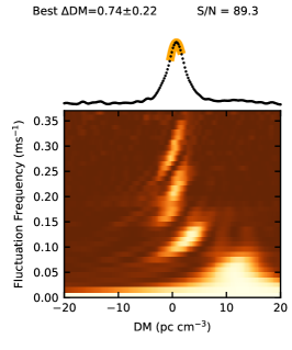
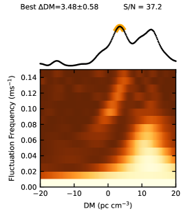
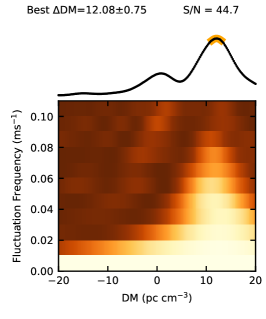
Does this correlation signify a causative relationship with the intrinsic brightness of the burst, and/or is it related to the method or to instrument noise? To investigate the effect of noise on the performance of DM_phase, we utilized a nine-burst sample of burst spectra that were made public by Xu et al. at the time of manuscript preparation141414 After our analysis was performed, an extended version of burst spectra sample from Xu et al. (2022) have been made public (Wang et al., 2023a). We will take burst #377 from Xu et al. (2022) as an example, and discuss other bursts afterwards.
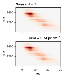
The observed behavior of burst #377 is shown in the top left panel of Fig. 4. It has three partly merged components and an overall drift in frequency. The spectrum of the -resolved power versus the trial DM shows different zones corresponding to these scales. If we now add Gaussian noise to each frequency channel of the data (pre-normalized by the standard deviation of noise in the off-pulse region), the fine temporal structure is washed out ever more, and above a certain amount of added noise only the low- feature remains. Above this edge in additional noise (i.e. below this boundary in terms of S/N), DM_phase aligns the entire spectrum, converging on a DM about 10 pc cm-3 higher that the original value. The step is clearly visible when comparing the middle column in Fig. 4 to the right column.
We note that even without such additional noise the DM derived with DM_phase depends on the choice of the frequency and time averaging, as well as the channel normalization method. The resulting spread of DM measurements is a few times larger than the estimated DM_phase uncertainties. The same level of discrepancy is observed between DMs from Xu et al. (2022) and our measurements. Also, on our normalized data we measure integrated S/N of about 1.5 times larger than reported by Xu et al. (2022). This could be partly attributed to normalization or, partly, be due to a finer grid of trial widths we used for the integrated S/N calculation. We also note that the some of the information in the header of burst spectra that accompany Xu et al. (2022) (e.g. DM and cardinal burst number) deviates from the corresponding entries in their data table.
How much the DM varies with pulse S/N, as well as the character of this variation (e.g., with or without a “step”), is determined by the temporal-spectral shape of the burst. The least amount of variation, less than a few times the DM_phase-reported error, was recorded for bursts with distinct, widely separated components (e.g. bursts #779, #1377, and #1398 from Extended Data Figure 6 in Xu et al. 2022). Mean while, bursts with an overall drift in frequency (e.g. #377, #460) exhibited steps of pc cm-3 even at integrated S/Ns as large as 100. Thus, for the majority of the burst population in Fig. 3 the DMs are likely overestimated if unresolved drift in frequency was present.
FAST provides by far the largest and brightest sample of bursts, since for other telescopes the S/N is usually smaller, meaning that DM overestimation is widespread. As this is a matter of S/N, the same effect will occur for very bright bursts observed with relatively less sensitive telescopes.
Assuming that the DM excess of Xu et al. is indeed due to absorption of the trombone effect, we can calculate the absorbed drift rate from an extra dispersion delay between the edges of the band. For a pc cm-3, the frequency drifts are between 25 and 225 MHz/ms, comparable to the values found by Zhou et al. (2022), who determine their DM values from a sample of bursts with sharp, separate components.
If the true DM at the time of the GMRT observations was 411 pc cm-3, then the DM measured from burst G05 would imply a drift rate of 8 MHz/ms (Fig. 5). It is useful to compare this value to the study of Marthi et al. (2022), who calculated drift rates for a sample of 48 FRBs recorded during a single session with the GMRT. In that study, a DM of pc cm-3 was determined using a singular-value decomposition of the spectrum of the brightest burst, exhibiting a sharp burst rise and a few partially merged components. All bursts in the study of Marthi et al. (2022) displayed trombone drift, with rates between 0.75 and 20 MHz/ms. We thus conclude that the DM determined for G05 has some drift absorbed in it.
For the F21 activity cycle, Zhou et al. (2022) measure an average DM of 412.4(3)–411.6(3) pc cm-3, using only those pulses that show sharp edges or well-separated components. Individual measurements are spread within pc cm-3, larger than the reported errors. Kirsten et al. (2024) measure DMs consistent with Zhou et al. (2022) for that day. Statistically, their DMs for the W22 cycle are no different from our measurements. Overall we conclude that reliably detecting any secular DM trend on the level of 1 pc cm-3 between activity cycles requires a more robust method of dealing with the influence of burst structure than is currently used.
4.2 (Quasi-)periodicity
Some FRBs consist of multiple components arranged in a seemingly regular fashion. A reliable detection of such (quasi-)periodicity may have interesting implications for FRB emission theories. For example, such periodicity may be a direct manifestation of the relatively fast spin period of an emitting compact object. Or, it may reflect the features of spark generation or non-stationary plasma flow in the neutron star magnetosphere (e.g., Mitra et al., 2015). Finally, quasi-periodicity of subpulse components appears naturally when FRB generation is driven by crust motion (Wadiasingh & Chirenti, 2020).
So far, the most reliable detection of periodicity comes from a one-off FRB. Chime/FRB Collaboration et al. (2022) detected a 217 ms periodicity in the nine components of FRB 20191221A. This periodicity is consistent with beamed emission from a neutron star rotating at 5 Hz. Other detections are close to the level and exhibit quasi-periods ranging from sub-milliseconds to tens of milliseconds (Pastor-Marazuela et al., 2023; Chime/FRB Collaboration et al., 2022).
FRB 20201124A presents an interesting example of a repeating FRB source characterized by apparent periodicity in some of its sub-bursts. Nevertheless, timing analysis of the sub-burst TOAs derived from 53 bursts within the F21 activity cycle, as conducted by Niu et al. (2022), did not reveal a single period with possible harmonics, but unveiled a broad distribution of periods spanning the range of 1 to 10 ms, with an extended tail reaching up to 50 ms. All identified periods exhibited significances not exceeding of the normal distribution.
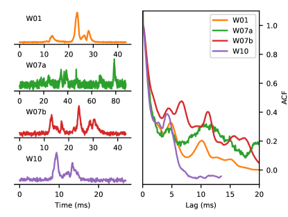
In our sample, only bursts W01, W07, and W10 exhibit multiple components with potentially periodic spacing. To test for this sub-second periodicity we computed the auto-correlation function (ACF) of W01, W10 and the two parts of W07 (Fig. 6), but no prominent periodicity was found. The quasi-periods corresponding to the peaks on ACF are in good agreement with the distribution obtained by Niu et al. (2022) on a larger sample of bursts.
We complemented the ACFs with a timing analysis, which may be more sensitive to short periodicities potentially buried in the zero-lag peak of the ACF. In the timing analysis, periodicity is searched for in the sample of sub-burst TOAs, and the accuracy of the timing analysis is greatly influenced by the precision of the TOA measurement. If sub-bursts have complex shape and are closely spaced, it becomes difficult to determine which parts of the time series belong to different sub-bursts, and which reflect the intrinsic shape of an individual sub-burst. An example of this can be seen in the sub-bursts of FRB W07 on the upper subplot of Fig. 7 around ms.
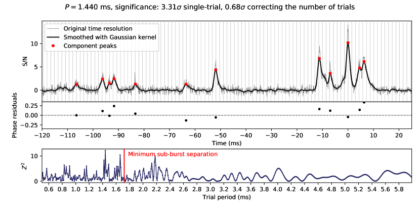
For the subsequent analysis, we defined each TOA as the time stamp of the peak on the signal smoothed with a Gaussian kernel with a five-sample standard deviation. The peaks were located using scipy.signal.find_peaks.
For bursts with prominent, ostensible quasi-periodicity it is logical to assume that the period is close to sub-burst separation or its integer multiplicative (e.g. FRB 20191221A in Chime/FRB Collaboration et al. 2022, where sub-bursts arrive every one or two periods). The situation becomes more complicated when bursts are less frequent, as in FRB 20201124A. Searching for periods around the minimum sub-burst component separation then leads to a large variation of these periods from one burst to another, as was demonstrated by Niu et al. (2022).
In what follows we thus do not assume that the minimum separation between sub-bursts strictly constrains the possible periodicity. Instead, we performed a uniform search over a grid of trial periods using the statistic:
| (1) |
where is the phase of ith sub-burst component computed with trial period . was maximized over the range of between 0.5 and 6 ms with an increment of 0.01 ms. We estimate the significance by repeating the analysis on samples of random TOAs, keeping the first and last fixed, and drawing the remaining TOAs from a uniform distribution spanning .
.
Applying this analysis to the 11-component burst from Niu et al. (2022), we find an optimal of 3.07 ms, . In the batch simulated of sets containing 11 random TOAs, 99.75% of sets had a maximum for ms. This equates to a significance for the observed burst equivalent to for a normal distribution. The results are close to those obtained by Niu et al.: ms with significance of 151515Differences may stem from inaccuracies in determining TOAs from the digitized version of their Fig. 7.. However, since we searched over a grid of , the number of trials should be taken into account. Comparing the maximum score of the real data to the pool of maximum scores lowers the significance to . Thus, for these weak signals the presence of a priori constraints on is crucial for obtaining a significant result.
Among the bursts in our sample, W07 exhibited quasi-periodicity with a period of ms, showing a significance of directly, and after correction for the number of trials. For Bursts W01, W10, and the two sub-burst groups of W07, no discernible periodicity with single-trial significances greater than was identified. It appears the sub-bursts lack prominent quasi-periodicity, at least when not considering sub-burst shape appropriately or in the absence of motivated constraints on .
Under the assumption that sub-bursts appear almost every period, and that can change from one burst to another, we examined the distribution of from Niu et al. (2022) in order to investigate whether the frequencies were clustered around specific harmonics, as predicted by the crust motion and low-twist theory (Wadiasingh & Chirenti, 2020). We did this by obtaining the eigenmode -number from the formula over a range of trials. For each trial we examined the deviations of the obtained values for from their respective nearest integer counterparts. These distributions appeared to be uniform and indistinguishable from the same distributions computed on sets of uniformly distributed random period values. Although no clustering was hence found, we cannot disprove crust motion theory this way. Since the eigenfrequency depends also on the strength of magnetic field at the location and time of the crust motion, it may vary from one burst to another (Wadiasingh & Chirenti, 2020).
4.3 Burst fluences
Tables 1 and 3 list the peak flux densities and fluences of the bursts recorded in this study. Prior to measuring the peak flux densities, the band-integrated time series were averaged by several time bins (see the caption of Fig. 2). For fainter bursts, the peak flux density depends on how much of such averaging was performed.
The fluence was estimated by summing the signal in a fixed-size window around the burst peak. For all bursts except W07, this window size comprised 60 ms. For W07 we used a larger window, from to 20 ms, to encompass all components. The fluence of W01 is in agreement with the CB17 detection we reported in Atri et al. (2022). For W07, we measure a 3 times larger fluence in the larger window, as we are now including the component group W07a, in contrast to the earlier reported results from the standard pipeline.
4.3.1 Fluence distributions
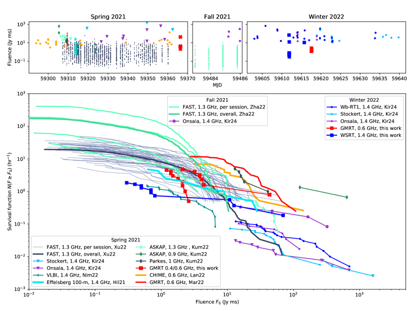
Statistical distributions of burst fluences provide valuable information about the FRB emission mechanism, and about propagation in the circum-burst environment (Cui et al., 2021; Xiao et al., 2024). Owing to the large number of bursts observed, FRB 20201124A has the potential to offer one of the best-measured distributions of burst fluences among repeating FRB sources. In practice, however, the distributions from different observations exhibit little agreement with each other (Fig. 8). The apparent mismatch is not entirely caused by the difference between the mean event rates at different epochs, but the shape of the distributions themselves seem to have intrinsic changes.
A series of dedicated observations by the FAST telescope demonstrated that the FRB 20201124A burst rate is highly variable (by up to two orders of magnitude), both within and between activity cycles (Xu et al., 2022; Zhang et al., 2022). The fluence distribution is bimodal (Zhang et al., 2022), but unfortunately, the pulse rate is insufficient for exploring any changes in the distribution shape on the timescale of the rate change, although some studies have been performed (Sang & Lin, 2023).
The fluences of bursts from WSRT observations fall within the range of fluences reported by other authors. Fainter bursts likely belong to the fainter component of the bimodal fluence distribution seen in the FAST observations Zhang et al. (2022). No contemporaneous observations were conducted during W22 activity cycle, however, and the position of the fainter component is known to shift from cycle to cycle. The WSRT-burst fluence distribution is flatter than normal, although similarly flat distributions have been recorded previously.
Bursts recorded by GMRT during the S21 and W22 activity cycles have steep fluence distributions. Bursts in our sample are, furthermore, generally fainter than the ones recorded with a similar observing setup by Marthi et al. (2022). The level of discrepancy between our two distributions and the one from Marthi et al. is, however, within the ranges observed by FAST.
4.3.2 Fitting methods
Generally, a cumulative distribution of burst fluences can be approximated with a power-law (PL) distribution, with a possible flattening at lower fluences, either intrinsic or due to sample incompleteness close to observational sensitivity limit. PL fits are easy to perform, have only few free parameters, and allow for quick comparisons with theoretical models (e.g. Wadiasingh et al., 2020). There are, however, limitations that should be kept in mind as these can bias the physical interpretation of the results.
One of the caveats concerns the fitting method. Historically, fluence distributions of individual pulses of pulsar radio emission have been approximated with PL functions by performing a least-squares linear fit to the survival function on a log-log scale (hereafter the “graphical method”), and this practice is still sometimes used for the FRB fluence distribution (Popov & Stappers, 2007; Bilous et al., 2022; Pastor-Marazuela et al., 2021; Kirsten et al., 2024). Despite the ostensible transparency of the graphical fitting method, the least-square minimization does not provide an accurate and unbiased estimate of the PL parameters – even if the number of the sample is quite large by FRB standards ( pulses, see Goldstein et al., 2004; Hoogenboom et al., 2006). A Maximum Likelihood Estimator (MLE) provides a much more accurate estimate of the PL index. In Appendix A we provide a detailed comparison of the two methods.
| Reference | Telescope | MHz | MJD start | min | min | max | # of FRBs | fraction PL | ||
| Spring 2021 | ||||||||||
| Lanman et al. (2022) | CHIME | 600 | 59177 | 0.24 | 3.2 | 5.8 | 140 | 33 | 0.88 | |
| Kumar et al. (2022) | ASKAP | 1271 | 59306 | 1.01 | 21.0 | 27.0 | 58.0 | 9 | 0.89 | |
| Xu et al. (2022) | FAST | 1250 | 59307 | 0.19 | 0.017 | 5.6 | 67.3 | 1715 | 0.08 | |
| Kumar et al. (2022) | Parkes | 850 | 59309 | 1.27 | 13.0 | 13.0 | 41.0 | 5 | 1.00 | |
| Marthi et al. (2022) | uGMRT | 650 | 59310 | 0.18 | 2.6 | 7.2 | 108 | 47 | 0.89 | |
| Hilmarsson et al. (2021) | Effelsberg | 1360 | 59314 | 0.22 | 0.6 | 1.1 | 28.1 | 19 | 0.63 | |
| Nimmo et al. (2022) | VLBI | 1400 | 59315 | 0.28 | 0.6 | 0.9 | 6.6 | 18 | 0.89 | |
| Kirsten et al. (2024) | Onsala | 1400 | 59327 | 0.26 | 13.3 | 13.3 | 693 | 8 | 1.00 | |
| This work | uGMRT | 400 | 59366 | 0.46 | 2.1 | 2.1 | 43.4 | 6 | 1.00 | |
| Fall 2021 | ||||||||||
| Zhang et al. (2022) all | FAST | 1250 | 59483 | 0.20 | 0.010 | 1.69 | 10.4 | 696 | 0.15 | |
| Zhang et al. (2022) | FAST | 1250 | 59483 | 0.09 | 0.020 | 0.020 | 5.4 | 31 | 1.00 | |
| Zhang et al. (2022) | FAST | 1250 | 59484 | 0.83 | 0.012 | 1.19 | 3.5 | 63 | 0.14 | |
| Zhang et al. (2022) | FAST | 1250 | 59485 | 0.27 | 0.010 | 1.61 | 10.4 | 190 | 0.20 | |
| Zhang et al. (2022) | FAST | 1250 | 59486 | 0.18 | 0.013 | 1.16 | 5.6 | 412 | 0.26 | |
| Winter 2022 | ||||||||||
| Kirsten et al. (2024) | Wb-RT1 | 1380 | 59603 | 1.16 | 13.4 | 224 | 699 | 24 | 0.17 | |
| Kirsten et al. (2024) | Onsala | 1400 | 59612 | 2.75 | 14.9 | 67.7 | 122 | 6 | 0.50 | |
| This work | WSRT | 1369 | 59612 | 0.19 | 0.3 | 0.3 | 69.6 | 10 | 1.00 | |
| This work | uGMRT | 650 | 59617 | 6.58 | 1.2 | 2.1 | 2.6 | 10 | 0.50 | |
| Kirsten et al. (2024) | Stockert | 1381 | 59619 | 0.65 | 11.0 | 36.1 | 250 | 13 | 0.69 | |
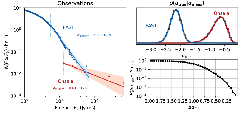
As an illustration, we refit the fluence distributions recently obtained by Kirsten et al. (2024) using both methods: graphical and MLE. The outcome of the original fits prompted the authors to speculate that there may be two separate populations of pulses emitted by FRB 20201124A, with the more energetic population having substantially flatter distribution. Unlike the authors, we fit fluences instead of spectral energy densities. While we use all available Onsala measurements, we necessarily exclude the Stockert observations from fitting with both methods, as the large difference in exposure time and sensitivity makes combining the datasets for subsequent MLE fitting very difficult. As in Kirsten et al. (2024), the optimal minimum fluence value for both the FAST and Onsala distributions was determined with powerlaw161616https://pypi.org/project/powerlaw/, modified according to Eq. 11-12 in Appendix A..
Despite the above-mentioned differences in approach, our implementation of the graphical method reproduces the values of the measured PLI and its corresponding bootstrapping errors as reported by Kirsten et al.: and .
The MLE method, however, results in and . Clearly, the MLE determines the errors to the fit to be larger than the graphical method indicates. As a matter of fact, the difference between the FAST and Onsala divided by errors added in quadrature, which is 13.7 for graphical method171717Bootstrapping errors are generally not well-suited for determining PLI uncertainties, see Appendix A., is only 4.7 according to the MLE. This indicates the difference in PLI between Onsala and FAST is much less significant when measured with MLE method.
However, the distribution of around true value is not Gaussian: obeys a gamma distribution, which deviates from a normal distribution for small sample sizes, . For a uniform prior on this results in the posterior distribution for being skewed towards steeper PLI for small . In Fig. 9 we show the posterior distributions for both the FAST and Onsala samples constructed from the fitted on a grid of trial . The posterior is well described by the gamma distribution from James et al. (2019) modified for the unbiased estimate (in their notation) by taking :
| (2) |
Having two posterior distributions, one may calculate the probability that the difference between the values for the FAST and Onsala samples is smaller than some threshold value (Fig. 9). These probabilities remain low for differences in PLI less than , indicating that, indeed, a significant difference exists between and . This significance is, however, appreciably smaller than implied by graphical method. For example, graphically, but according to the MLE.
To summarize our findings up to here, accurate estimates of the PLI for small burst samples critically depend on two factors: first, using an unbiased PLI fitting method, and second, taking into account the skewness of the posterior probability distribution.
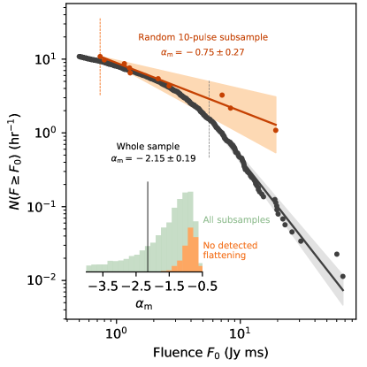
There is, however, one more caveat connected to sampling from flattened distributions. If the observed fluence distribution flattens at the low end, either due to instrument sensitivity, or intrinsically, then this flattening can not always be recognized in small samples, and the measured power-law index (PLI) can be biased towards shallower values. The amount of this bias depends on the extent of flattening. As an example, we show the distribution of 10-pulse PLIs from the FAST S21 sample in Fig. 10. The sample was truncated at 5 Jy ms and the flattening signifies an intrinsic property of the pulses. The PLI distribution is skewed towards shallower values, which is expected because low-fluence pulses with shallower survival functions are more abundant. However, about 17% of these 10-pulse samples do not exhibit apparent flattening at the lower-fluence edge of survival function. Their survival functions are well-fitted with a single PL for the whole extent of the 10-sample distribution. A chance observation resulting in one such 10-burst realization may well lead to the erroneous conclusions that the distribution of burst fluences obeys a PL with a shallow index, and to a subsequent unfounded scientific interpretation.
The exact amount of PLI bias towards shallower values depends on the sample size and on the underlying fluence distribution as observed with a specific instrument under a specific setup. Assumptions about intrinsic fluence distribution as well as models of instrumental limitations (see e.g., Gardenier et al., 2019; Wang & van Leeuwen, 2024, for such models) should both be taken into account while interpreting the measured PLIs.
4.3.3 Fitting results
In this section, we review the PLI measurements for the fluence survival functions of bursts recorded in our observations and reported in the literature. Table 4 summarizes the results of the MLE fitting procedure. Unlike Kirsten et al. (2024), we did not combine bursts recorded by different telescopes, and we did not correct for the unknown possible underestimation of CHIME fluences (Lanman et al., 2022). For the FAST sample and our WSRT observations, we combined bursts with separation smaller than 100 ms to facilitate comparison with (Kirsten et al., 2024). Such proximity threshold lies within the short-recurrence component of the bimodal waiting time distribution and is smaller than the 400-ms sub-burst separation threshold in Zhou et al. (2022), which was derived from the trough between the two components of the waiting time distribution. In practice this means that for the small fraction of bursts the fluences of individual sub-burst clusters, as defined by (Zhou et al., 2022) were counted separately. This, however, had only minor influence on the shape of fluence distributions.
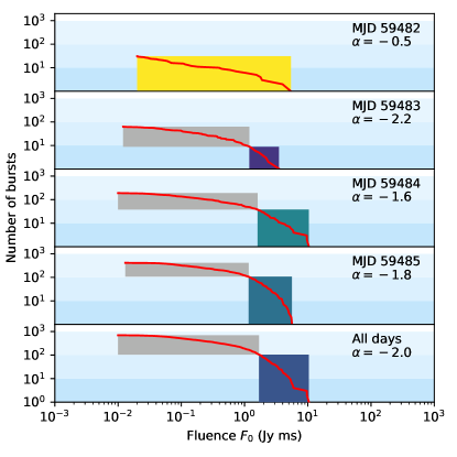
In Table 4, all measured values, except one, are within the range of to . However, we must warn the reader that nominal PLI values, even with their respective MLE fit uncertainties, should be treated with caution due to the apparent flattening of distributions at the lower-fluence end, which can be either instrumental or intrinsic. To illustrate this, we show the powerlaw fit for four individual sessions of the F21 FAST burst sample (Fig. 11). During the observing run, the rate of pulses increased more than tenfold, from 31 to 412 combined bursts per one-hour session. The overall shape of the fluence distribution did not change dramatically, yet for the first session, the PL fit yielded a flat without a low-fluence cutoff. For the subsequent sessions, the optimal fit excluded the low-fluence region, resulting in a much steeper PLI. It is possible that the shallow for the first session is solely due to the aforementioned bias present in small samples drawn from a flattened distribution; however, intrinsic variability cannot be ruled out.
The fits for per-session fluence distributions of the FAST sample from the S21 activity cycle also exhibited a dependence on the number of bursts recorded per session. The number of bursts varied from 11 to 99 per session. The measured PLIs were more diverse for smaller burst samples, ranging from to , with occasional much steeper outliers of about . The fraction of power-law-obeying bursts ranged from 5% to 90%, with steeper indices corresponding to larger minimum fluences and a smaller number of bursts in the PL tail. The two most prolific sessions, with more than 80 FRBs each, yielded values of and , with 25% of bursts belonging to the PL tail.
All three burst sub-samples in our study are small, with ten or fewer bursts each. The bursts from two GMRT sessions in the S21 and W22 activity cycles resulted in dramatically different values, and . The very steep PLI resembles similar steep values of the Spring FAST per-session fit when the burst sample size was small, and a relatively large minimum fluence was found for the PL tail. The shallower of the S21 cycle is largely determined by a single bright burst, G05. Similarly, our for the CHIME data is shallower than the MLE fit from Lanman et al. (2022), as they excluded the brightest burst due to uncertainties in fluence determination. The WSRT burst sample is described by a shallow distribution with and no apparent low-fluence flattening. This PLI is close to the ones reported by Kirsten et al. (2024) and Hilmarsson et al. (2021), but extends to smaller fluences.
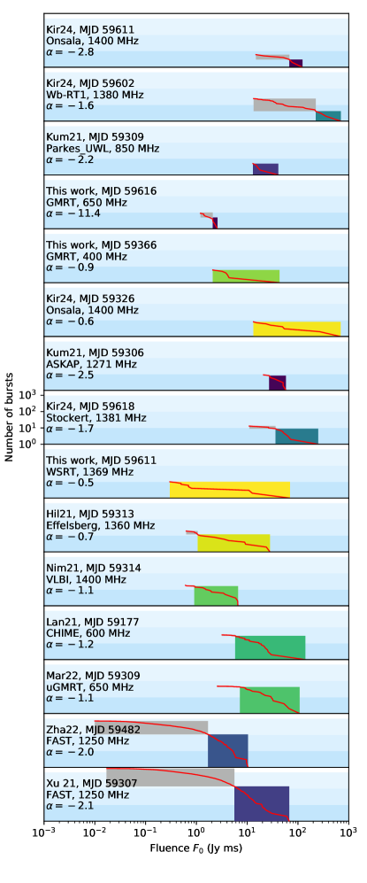
Fig. 12 provides a graphical representation of the PLI measurements from Table 4. Burst samples are sorted by the number of bursts in the PL tail. Overall, PLIs determined from burst samples smaller than about a hundred tend to have diverse values that are inconsistent between different studies. For the largest sets of pulses (696 and 1715 FRBs from the two FAST studies), only a small fraction (about 10%) of the brightest pulses follow a power-law distribution, with close to and minimum fluence differing by a factor of 3. Since these observations were performed under the same observing setup, the difference signifies intrinsic variability between activity cycles.
Given the inevitable instrumental bias, possible intrinsic frequency evolution and temporal variability, constraining the PLI is a daunting task. One can also well ask the question whether PL approximation should be used in this case at all, since for both of the two samples of bursts that were largest and most sensitive, only 10% of bursts have fluences that obey a PL distribution.
4.3.4 Fitting code availability
To facilitate the future use in the community of the correct, MLE algorithms for fitting burst fluences, we have made available an ipython notebook that implements the various types of PL fits. It includes instructions on how to adapt the powerlaw package as described in Appendix A. The notebook is hosted on Zenodo181818https://doi.org/10.5281/zenodo.12644702 and GitHub191919https://github.com/TRASAL/FRB_powerlaw.
4.4 Scintillation
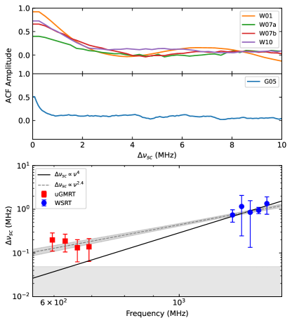
In order to measure the decorrelation bandwidth, we obtained the spectra of the brightest bursts in our sample, G05, W01, W07A, W07b, and W10, by averaging their emission in time over the time bins where the signal is four times larger than the noise standard deviation. Note that for W07a, only the last, brightest component satisfies this criterion. For each ALERT burst, we removed the data above MHz, where RFI becomes strong in the observations. For the uGMRT burst G05, we fitted the burst spectrum to a Gaussian and only took the frequencies within two standard deviations of the center in order to have enough signal for the analysis; this is between 580 MHz and 709 MHz. Next we compute the ACFs of the spectra, removing the zero-lag frequency value, and fit the central peak of the ACF to a Lorentzian. The decorrelation bandwidth is often defined as the half-width at half-maximum of the ACF’s fitted Lorentzian (see e.g. Lorimer & Kramer, 2005, Section 4.2.2). For the ALERT bursts, we obtain an average decorrelation bandwidth (weighted by the inverse standard deviation of each measurement) MHz at the central frequency 1336.5 MHz. For G05, we obtain MHz at the central burst frequency, 644.5 MHz.
The frequency-dependent intensity variations produced by scintillation are expected to follow a power law evolution of the form , with the frequency in GHz, a constant that gives the decorrelation bandwidth in MHz at 1 GHz, and the scintillation index, expected to be for scintillation produced by a thin screen and for scintillation produced in an extended, turbulent medium. To measure the power law index of the decorrelation bandwidth, we divide the bandwidth into several subbands, and we measure the half width at half maximum (HWHM) in each subband as described above. We divide the Apertif bursts into five subbands, and the uGMRT one into four. For the Apertif bursts, we compute the HWHM weighted average in each frequency subband, and then we fit all decorrelation bandwidths as a function of frequency to a power law spectrum. We obtain MHz, and . The results from the scintillation analysis are presented in Fig. 13.
Our measurements at both frequencies are based on a small number of bursts. Previous studies have shown that both the decorrelation bandwidth and vary substantially when measured on individual bursts within a relatively narrow bandwidth of 500 MHz centered around 1250 MHz: Xu et al. (2022) reported a mean of 4.9 with a standard deviation of 6.4. This variation may be at least partially influenced by the intrinsic spectral structure of the bursts. Inferring from the combined spectra of a few dozen bursts detected within an hour-long observing session resulted in a more shallow of (Zhou et al., 2022).
Main et al. (2022) increased the robustness of determination by comparing decorrelation bandwidths at 700 and 1400 MHz. Their setup is similar to ours in terms of frequency coverage, but their sample of bursts is larger. They reported a power-law index of , which is also shallower than the one for the thin screen model. However, both in our measurements and those from Main et al. (2022), the decorrelation bandwidth at the lowest radio frequencies may be biased by insufficient frequency resolution, resulting in being biased towards more shallow values.
The study of Main et al. (2022) utilized bursts from the S21 activity cycle, with low- and high-frequency observations conducted several days apart. Our measurements at 1.4 GHz come from the W22 cycle, 245 days after the S21 observations at 650 MHz. Wu et al. (2024) reported small annual variations in the observed decorrelation bandwidth attributed to the Earth’s movement with respect to a moderately anisotropic scattering screen located in the Milky Way (see also Main et al., 2022). This variation is much smaller than the scatter associated with measurements from individual sessions and therefore can not be the main source of systematic uncertainty in our measurement. The available bulk of observational data does not show evidence for a secular trend in the decorrelation bandwidth or across three activity cycles.
Main et al. (2022) detected enough nearby bursts from FRB 20201124A to measure its scintillation timescale of min in the L-band. Unfortunately, the most closely spaced bursts with sufficient SNR in our sample (W01 and W07) are separated by min, which does not allow us to probe the scintillation timescale of the source. The correlation coefficient between W01 and W07a/b is close to zero, consistent with the previous measurement.
4.5 TOA statistics
The similarity in burst arrival statistics between FRBs and the high-energy short bursts from magnetars was one of the key observational facts put forward by Wadiasingh & Timokhin (2019, hereafter: WT19) in support of their crust motion and low-twist model of FRB generation. Both observed burst types feature a log-normal distribution of waiting times, and a log-uniform distribution of TOAs as measured from the outburst start time. WT19 studied the distribution of burst arrival times using a sample of 93 FRBs from FRB 20121102A recorded over the span of five hours. Some of the FAST observations of FRB 20201124A provide much higher a pulse rate (up to a few hundred pulses per hour), but the duration of the observing session is smaller, typically less than two hours.
Using the publicly available information about burst fluences and arrival times from Xu et al. (2022) and Zhang et al. (2022), we constructed the distribution of waiting times between successive bursts. As mentioned before, this distribution consists of two non-overlapping log-normal components. Based on a common definition of sub-bursts, we combined bursts which were separated by less than 400 ms into one, using an iterative routine. For each resulting cluster of sub-bursts, the TOA was taken to be the time of arrival of the first burst, and the cluster fluence to be the sum of the individual component fluences. Combined bursts from each observing day were analyzed separately.
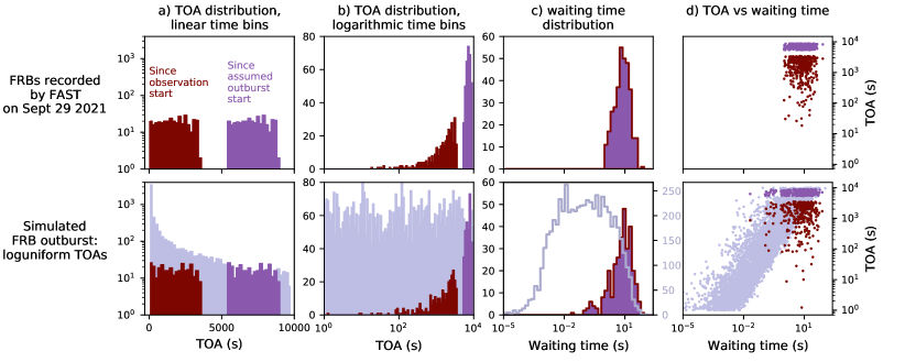
Fig. 14 shows the distribution of burst TOAs measured with respect to the session start for the most prolific observing session, on September 29 2021 (MJD 59486; see Table 4). The distribution is uniform with linear time bins and, unlike for FRB 20121102A (WT19), there is no linear correlation between the logarithms of the TOAs and the corresponding waiting times (the brown points in the top-right subplot). This discrepancy can, however, be explained if the observation took place some time after the outburst started, when the burst rate no longer changed significantly during a session.
To illustrate this, we simulated burst arrival times by generating log-uniformly distributed random variables , using scipy.stats.loguniform. These random variables fell within the range of s with a probability density function of Approximately 1.5 hours after the start of the simulated outburst, the rate of occurrence for remains relatively constant over the duration of the FAST session.
If TOAs are measured from the start of the simulated outburst, s, their statistics closely resemble the statistics of real bursts (Fig. 14). This suggests the possibility that the observed bursts are part of an outburst that began several hours before the observations. In this model, the variation in the session-to-session burst rate, which shows significant growth towards the end of the F21 activity cycle, could be attributed to different outbursts overlapping, or occurring in close succession. Unfortunately, the scope of this work does not permit a quantitative assessment of the probability of FAST missing the start of an outburst after observing FRB 20201124A for almost 60 days with duty cycle. Such an assessment would require an estimation of the tentative duration of an outburst and the frequency of their occurrence.
4.6 Frequency-dependent activity cycle
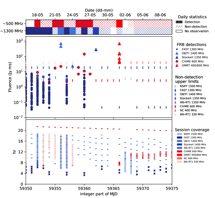
FRB 20201124A was extensively observed, by multiple telescopes, around the end of the S21 activity cycle. Figure 15 provides a summary of the time/frequency coverage of these observations, including the TOAs and fluences of the detected FRBs, plus fluence upper limits for any non-detections.
The majority of the FRB detections in the L-band were provided by sensitive FAST observations. These observations occurred at intervals of 1 or 3 days, with each 2-hour session yielding the detection of dozens of bursts with fluences above 0.053 Jy ms. Notably, there was an abrupt cessation of emission between MJD 59360 and 59363, after which no FRBs were recorded despite the unchanged observing setup and cadence.
These FAST observations were complemented by Kirsten et al. (2024), who conducted near-daily observations using several smaller telescopes. Their observations necessarily featured a significantly higher detection threshold, approximately 10 Jy ms. The last known pulse from the S21 session, detected by Kirsten et al., occurred on May 28, one day before the first non-detection by FAST, on a day when FAST was not conducting observations.
Shortly after this then yet unbeknown quenching, Mao et al. (2022) executed an extensive targeted search for bursts from FRB 20201124A in the L-band using the Nanshan 26-m radio telescope (NSRT). The authors determined a minimum detectable fluence of 4 Jy ms. On June 02 and 03, when FAST was not observing, the NSRT sessions were significantly longer than those generally used at FAST. If the source had persisted as active as before, several bright pulses should likely have been detected on these dates – but none were. On June 07, both NSRT and FAST observed FRB 20201124A, a few hours apart, with neither telescope detecting any bursts.
At the lower frequencies centered around 400 to 600 MHz, the majority of observations are provided by CHIME/FRB. That transit instrument records FRB 20201124A for 3.13 minutes virtually every day in the frequency range of 400–800 MHz. Lanman et al. (2022) estimate the burst rate after March 20 to be between 0.9–2 100 day-1, and the bursts exhibit Poissonian repetition. No bursts were detected in the five sessions between May 27 and our GMRT detections described below; this absence has a Poissonian probability of between 0.11 and 0.37, assuming constant observing and instrument conditions. Beyond purely Poissonian variations, it is noteworthy that the rate may also intrinsically vary on timescales shorter than a month, as indicated by the apparent inconsistency between the rate derived from CHIME/FRB observations and that from a 3-hour April session at 550–750 MHz at GMRT (Marthi et al., 2022). For the CHIME/FRB fluence limit, we take the lowest-fluence burst detection from Lanman et al. (2022), namely 3 Jy ms.
Trudu et al. (2022) observed FRB 20201124A at similar frequencies, 400–416 MHz, with the Northern Cross (NC) radio telescope, for 68 hours in April and June 2021. The authors estimate a minimum detectable fluence of 44 Jy ms and expect bursts to be detectable over this whole observing campaign. That expectation is based on the rates and the power law fluence distribution slope from CHIME/FRB monitoring (Lanman et al., 2022), and assuming there is no burst rate variability. Similarly, Kirsten et al. (2024) observed FRB 20201124A at 350 MHz with Wb-RT1 during several days, right before the L-band quenching, with an estimated minimum detectable fluence of 42 Jy ms, and not detecting any bursts.
Our observations with GMRT yielded six bursts on 2021 June 01, all of them with fluences above 40 Jy ms and one burst reaching fluence of 680 Jy ms. FAST observed FRB 20201124A a few hours before these GMRT observations and placed a stringent Jy ms upper limit on the FRB fluences in L-band.
Taken together, these detections and strict upper limits show that after it stopped emitting at L-band, FRB 20201124A continued to produce bursts at 400 to 600 MHz. The evidence is shown in Fig. 15. We estimate that the low-frequency radio emission may have lasted for 3–6 days after bursts stopped in L-band. The lower limit of 3 days comes from a scenario where the L-band quenching happened right before FAST observations on May 29, and lower frequency emission ended right after the GMRT observations on June 01. The upper limit of 6 days follows from assuming the high frequencies cease right after the last detected Stockert burst on May 28 and low-frequency emission persist up to the non-detection session at the Northern Cross telescope on June 03.
So far, only FRB 20180916B is known to display a similar frequency-dependent activity window in a repeating FRB (Pastor-Marazuela et al., 2021; Pleunis et al., 2021b). This source has a well-determined activity period of 16.3 days (CHIME/FRB et al., 2020). From comparing the activity phase-resolved burst detection rate in simultaneous observations using WSRT/Apertif and LOFAR, and in earlier CHIME/FRB observations, the authors conclude that higher frequencies appear to arrive earlier in phase. This trend was confirmed to extend to frequencies as high as 5 GHz. Between 150 MHz and 5 GHz the center of activity window shifts by about 6 days and the width of the window shrinks from 3.6 to 1.0 days (Bethapudi et al., 2023).
For FRB 20201124A, the activity window is challenging to determine precisely because of the uneven observational coverage, but evidence suggests that its duration is highly variable, with the duration of the inactive sessions ranging from a few months to at least two years (Lanman et al., 2022), and the active stages spanning months. Targeted searches have ruled out a periodicity of up to 10 days (Xu et al., 2022; Niu et al., 2022; Du et al., 2023), but longer periods are not yet disproven.
5 Geometric constraints on emission regions
In the low-twist magnetar model of FRB generation, bursts are produced in the magnetosphere of a neutron star via a pulsar-like emission mechanism (WT19). The exact nature of that invoked mechanism remains a long-standing mystery despite a plethora of observational pulsar facts and decades of ongoing modeling efforts. Nonetheless, the key observational properties of pulsar radio emission can be explained by a pair of phenomenological models, known as the radius-to-frequency mapping (RFM; Cordes, 1978) and the rotating vector model (RVM; Radhakrishnan & Cooke, 1969). These models produce constraints on the overall magnetospheric geometry and the location of emission regions, based on a set of plausible assumptions. Below we will apply RFM/RVM techniques to bursts from FRB 20201124A.
5.1 Radius-to-frequency mapping (RFM)
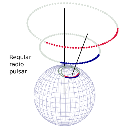
The RFM model postulates that radio waves decouple from magnetic field lines at a certain altitude, and propagate tangentially to the local magnetic field line at the decoupling point. We will call this the “emission point”, although radio waves may actually be produced elsewhere (Philippov et al., 2020). Lower radio frequencies are related to emission points situated higher in the magnetosphere, where the dipolar field has diverged further, offering a natural explanation for the broadening of the on-pulse window at lower frequencies that is observed in radio pulsars. In pulsars, the on-pulse activity window is thus frequency dependent, and wider at lower frequencies.
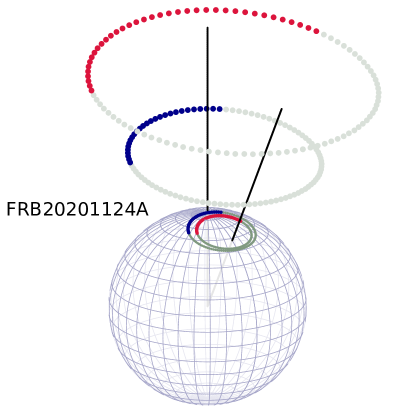
Now, the presence of similar frequency-dependent activity window behavior is evident in both FRB 20201124A and FRB 20180916B. Nevertheless, a clear distinction arises in terms of timescale: in pulsars, the widening amounts to fractions of a second, whereas for FRB sources, the frequency-dependent edge of the activity window extends over the course of days. However, the difference in spin phase remains consistent between radio pulsars and FRB repeaters if the latter are ULPs with spin periods () of weeks or longer.
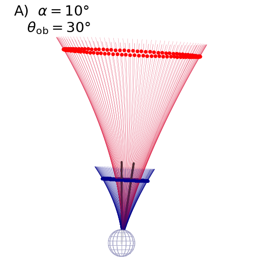
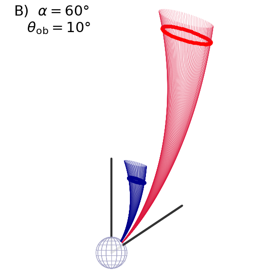
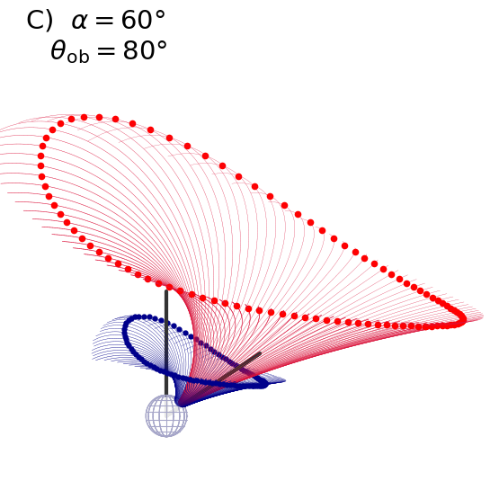
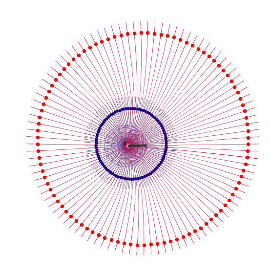
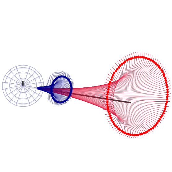
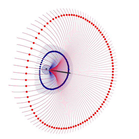
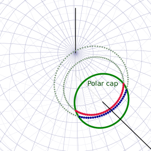
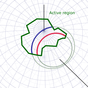
Qualitatively, the frequency-dependent edge of the activity cycle can be explained as follows: while the rotation of the magnetar slowly moves our line of sight (LOS) through the magnetosphere, we detect radio waves from field lines with footpoints in the active regions on the stellar surface. Plasma propagates along the active field line and generates radio emission of continuously decreasing frequency as it moves outward. Since this emission is highly beamed and its frequency is altitude-dependent, at any given moment of time the observed broadband spectrum is composed of radio waves coming from a range of altitudes and originating from different field lines. Consider, for clarity, only two radio frequencies – high and low. We, the observer, detect emission along our single LOS. But the two different frequencies originate from field lines with footpoints that form two separate, different paths on the surface of the star. These two paths may cross the edge of the active region at different times. Fortuitously, the low-frequency path may stay longer in the active region, resulting in detection of low-frequency FRBs after the cessation of higher-frequency emission. Since the effect is purely geometrical and there are no constraints on the shape of the active region for FRB 20201124A, many exact lags between high- and low-frequency quenching are possible, including negative lags, where low-frequency ceases first. The lags may also vary from one episode of activity to another. Once accumulated, the statistical distribution of lag magnitudes and signs may provide clues for the magnetospheric geometry configuration and the spread of the active regions on the stellar surface.
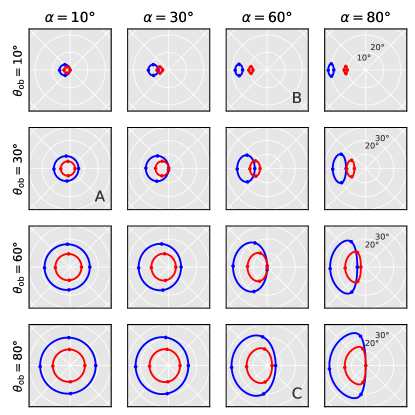
That is the qualitative description to introduce the underlying concepts. In what follows we will constrain the location of observable field line footpoints quantitatively. We assume the external magnetic field to be dipolar, designating the angle between spin and magnetic axis as . Since no external constraints are known for we take it to belong to a grid of trial values ranging from to and spaced by .
In a spherical coordinate system aligned with the spin axis, the observer LOS is defined by a pair of longitude/latitude angles. The latitude (also called “viewing angle”) does not change with time while the longitude corresponds to the spin phase at the moment of time : . In the absence of any external constraints, we review a grid of ranging from to with the spacing of .
Mathematical expressions for the dipolar magnetic field have the simplest form in the rest frame of the pulsar with magnetic moment directed along . In this coordinate system the location of the emission region is (, , ). The relationship between (, ) and (, ) is set by the requirement of the tangent to the magnetic field line at the emission point to be aligned with the LOS at the spin phase . Following Lyutikov (2016):
| (3) |
and
| (4) |
The coordinates of the footpoint of an active field line (, ) can be obtained using the equation for that dipolar field line in the rest frame:
| (5) |
and
| (6) |
Without constraints on the emission altitude , multiple field lines can contribute to the emission at any given . To maximize the stellar surface area under consideration in our exploration, we set the altitude of the observed higher-frequency radio emission to the smallest possible value. For the frequency at the center of WSRT band, this value corresponding to the minimum altitude from which radio waves can escape the low-twist magnetosphere. Assuming characteristic values of the limiting twist and crust oscillation frequency, and taking surface magnetic field to be G, we find this minimum escape altitude is (WT19, Beniamini et al., 2020).
While our numerical calculations are grounded on the assumption that the observed radio waves originate from curvature radiation (Wang et al., 2019, and references therein), the outcome is qualitatively similar when employing a different relationship between the radio wave frequency and the altitude of the emission region. For curvature radiation, the relationship between the radio frequency and the plasma/magnetic field parameters is as follows:
| (7) |
where is the Lorentz factor of the emitting particles, is the speed of light, and is the curvature radius of the field lines. For a dipole magnetic field, can be calculated from the coordinates of the emission point in the rest frame of the star:
| (8) |
Combining Eqs. 3–8, we obtain (, , ) for both the WSRT and GMRT radio frequencies and , for a range of chosen inclination and viewing angles. If does not change between two frequencies (Wang et al., 2019), over the entire range of input parameters. This next determines the low-frequency emission to take place at , above the minimum escape altitude of for GMRT frequencies. If , then is closer to , and the lower-frequency moves closer to its higher frequency counterpart.
The absolute value of (if taken constant between two frequencies) varies from to , with the higher values corresponding to field lines closer to the magnetic pole. These values are similar to the adopted by Wang et al. (2019). We note that our values of are lower limits, since we adopted the smallest possible .
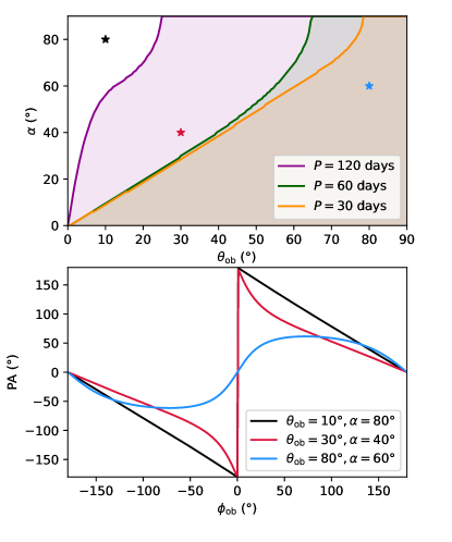
In the absence of any other constraints, the footpoints of the field lines with emission visible to the observer form a closed loop on the star surface (Fig. 16). For the chosen frequencies and , loops subtend of star surface for small , regardless of inclination angle. The fraction of the stellar surface encircled by this footpoint loop increases with growing , reaching about 20% for large viewing and small inclination angles.
Since the footpoint loops are closed, there exists a field line that can potentially provide radio emission at any spin phase . Whether this line will actually emit is determined by physical requirements for pair production and radio wave generation. For radio pulsars, such a requirement is that radio emission is produced by the open field lines with , where is the radius of the polar cap. Figure 18 provides an illustration of this, showing an example of the footpoint loops at two radio frequencies for an inclination angle of and . For plotting convenience, was set to be and . The polar cap with cuts segments from the footpoint loops, with the lower-frequency segment spanning a larger amount of spin phase bins. This implies that radio emission at lower frequencies is observed at earlier and later than the high-frequency one – the average pulse profile is wider at lower frequencies.
In the WT19 model the FRB 20201124A emission can originate on closed field lines, eliminating the polar cap requirement. The minimum emission altitude requirements imposed by the plasma transparency set limits on the magnetic colatitude , defined by , indicating that and for lower and higher frequencies, respectively. This broad region may host several active patches during the activity cycle.
A frequency-dependent activity edge arises when the LOS crosses the edge of the active patch. The exact lag between high- and low-frequency quenching is determined by the ”skewness” of the active region shape in the magnetic longitude direction and the unknown value of the spin period. For instance, assuming the FRB 20201124A spin period to be 2 months (the duration of the S21 activity cycle), then – for a 3–6 day lag, which translates to a similar upper limit on , with the latter being smaller for non-concentric footpoints loops. Thus, a small variation in active region shape may lead to a large variation in observed cessation lag.
A frequency-dependent activity window places constraints on the overall size of an active surface area. Individual crustal motions, on the other hand, are limited in size by the trombone frequency drift (Wang et al., 2019; Bilous et al., 2022; Lyutikov, 2020). Such frequency drift by MHz at 1400 MHz or by 125 MHz at 650 MHz would translate to . If the size of the active “spark” which produces an individual FRB is comparable to the amplitude of footpoint dislocation , then the latter is less than 500 m, below km from Beniamini et al. (2020).
5.2 The rotating vector model (RVM)
In the rotating vector model, the plane of the linearly polarized part of the radio emission is defined by the field line curvature plane at the emission point. For an inclined dipolar field, the position angle (PA) has a characteristic S-shape dependence on the spin phase and the angles introduced previously, as defined by the following analytical relation:
| (9) |
For both normal radio pulsars and magnetars, individual pulses exhibit a large diversity of PA behavior (Mitra et al., 2016; Johnston et al., 2024; Kramer et al., 2007). While numerous deviations are known (Johnston et al., 2023), the measured single-pulse PAs average to an S-curve defined by Eq. 9 in a considerable number of cases.
If we refocus now on FRB 20201124A, we see that the behavior of the PA curve is known only for a four-day stretch at the end of the F21 activity cycle (Jiang et al., 2022): there, the average value of the mean PA within the burst, weighted by burst energy, remained constant. The authors do not specify the limits of the constancy, but the distribution of mean PAs in Jiang et al. (2022) has a standard deviation of about . For the purpose of the arguments following below, we adopt a PA-gradient upper limit of per four days as best describing the observations.
We proceed by selecting (, ) pairs for which there exists at least one spin longitude window that can produce the observed . The size of the spin window depends on the unknown spin period, so we explore three trial periods, of one, two, or four months. Figure 19 shows the allowed ranges of inclination/viewing angles. For the smallest trial period of one month unless the inclination angle is close to . This excludes the non-concentric types of footpoint loops that are visible in Fig. 16. The inclination angle becomes less constrained as the potential spin period grows. Combinations of large and small (e.g. and ) still, however, produce a PA gradient that is too steep, even if months.
6 Summary and conclusions
FRB 20201124A is a prolific source of FRBs. Its bursts exhibit rich and complex structure and are undoubtedly capable of providing valuable insights into the underlying emission physics and propagation mechanisms. However, the current body of observational evidence contains gaps in areas of high scientific interest, and is inevitably affected both by instrumental and processing limitations.
6.1 Determining DM and fluence changes requires careful analysis
One example of these limitations is our current inability to disentangle the dispersive delay imposed by the interstellar medium from the intrinsic burst properties. We have demonstrated that the DM measured using the de-facto standard, structure-maximizing method absorbs the trombone drift for fainter pulses, leading to an overestimation bias in DM measurements that can be as large as 10 pc cm-3 – even for bursts with an integrated S/N on the order of 100. For brighter bursts, the complex structure often can not be maximized with a single DM value (e.g. Zhou et al., 2022). This bias should be taken into account while analyzing DM distributions aggregated from several studies with different sensitivities, since it can lead to apparently multimodal DM distributions which can subsequently be interpreted as plasma lensing or frequency-dependent DM (Wang et al., 2023b). On the other hand, directly incorporating external constraints on spectro-temporal FRB behaviour would allow for testing interesting physical effects. One example is investigating the filamentation of FRBs in the relativistic winds of magnetars, which implies a dependence of the measured DM on pulse luminosity due to propagation in the near-source environment (Sobacchi et al., 2023).
We confirm the absence of secular DM trends between different activity cycles of FRB 20201124A down to the level of a few pc cm-3. This places a limit on any electron density changes along the LOS, that could have been caused by an active circum-burst environment (Metzger et al., 2017). Combining WSRT bursts from the W22 cycle and burst G05 from the S21 cycle, we obtain a broadband PL dependence of the decorrelation bandwidth, more shallow than expected for Kolmogorov turbulence and close to the measurements of Main et al. (2022), who had a similar observing setup.
Despite the relative abundance of available data, the FRB 20201124A burst-fluence distribution remains poorly constrained. The FAST observations demonstrate there is a significant amount of variability in the fluence distribution, over a range of time scales: from between subsequent days to from between distinct activity cycles (Xu et al., 2022; Zhang et al., 2022). Corroborating the findings of Kirsten et al. (2024), we observe a shallower PLI for bursts in the W22 activity cycle than in the FAST measurements during previous cycles (all at the frequencies, around for 1300 MHz). However, as we demonstrate, PLI measurements tend to be imprecise and biased for small burst samples, especially when drawn from distributions with flattening at the low-fluence end, even if the observed distribution appears to be well-fitted with a single PL.
6.2 A ULP magnetar model for the burst behavior
We explore the possibility that FRB 20201124A is an ultra-long period magnetar with a spin period on the scale of months, a period that may remain undetectable for current searches. For such ULP sources, FRBs could be triggered by motion in the star crust, if these cause dislocation of magnetic field-line footpoints that leads to the production of plasma, which subsequently emits radio waves via some pulsar-like emission mechanism (WT19). Similar to the short X-ray bursts thought to be triggered by similar crustal motion events, the arrival times of individual FRBs would then follow a log-uniform distribution if measured from the trigger moment. Such a distribution has been reported for the repeating source FRB 20121102A (WT19). We demonstrate that TOAs of individual bursts from FRB 20201124A in both the S21 and F21 FAST samples exhibit a distribution that is uniform, not log-uniform. The sample could, however, still actually be part of the tail of a log-normal distribution, from a trigger event that occurred before these FAST observing sessions. As the burst rate, in a crescendo, increases exponentially before the emission quenches at the end of the F21 cycle (Zhang et al., 2022), there must be multiple trigger events during a single activity cycle. If these occurred several hours before the observation, our data is consistent with this model.
Another prediction from the crust motion and low-twist theory links crustal oscillations to quasi-periodic sub-burst spacing within individual FRBs. Our WSRT sample contains three bursts with seemingly periodic components; however, we were unable to find any significant periodicity. We show (and caution) that detecting periodicity for closely spaced sub-bursts of arbitrary shape is difficult, especially when the number of period trials is unconstrained.
If radio emission originates from only one frequency-dependent range of heights, then at any given spin phase, the LOS samples only a small fraction of the stellar surface. In contrast, X-ray bursts can be detected from the entire stellar surface at any moment. This difference may explain the intriguing result obtained by Tsuzuki et al. (2024), who found that regular radio pulses from the occasionally FRB-emitting magnetar SGR 1935+2154 exhibit correlation properties similar to those of extragalactic FRBs (Totani & Tsuzuki, 2023) and earthquakes. However, X-ray bursts from the same source did not show such correlation properties. We hypothesize that the lack of correlation for X-ray bursts stems from the superposition of several starquake events occurring simultaneously at different locations. In radio, individual starquake events are observed sequentially.
6.3 The FRB 20201124A activity cycle ends chromatically
At the end of the S21 cycle, our GMRT observations recorded several strong bursts at 300–600 MHz. That is surprising because only a few hours before, FAST had placed upper limits on the absence of emission at 1250 MHz that were 1000 times more stringent. By combining burst detections and telescope scheduling information, we are able to paint a complete, multi-frequency picture of the end of this activity cycle. We show that the edge of the S21 activity cycle depends on the observing frequency – low-frequency emission is present for 3–6 days after the higher-frequency quenching. This marks the second detection of a chromatic activity cycle for a repeating FRB source, following FRB 20180916B (Pastor-Marazuela et al., 2021; Pleunis et al., 2021b). However, for FRB 20180916B, a 16.3-day periodicity is known, and the chromatic window was established by combining bursts from several periods, whereas for FRB 20201124A, we have so-far recorded only a one-time event. Unfortunately, the end of the F21 and W22 activity cycles was not covered by multi-frequency observations.
The fact that lower-frequency emission has been recorded a few days after the disappearance of the higher-frequency one would be hard to explain within the plasma lensing theory of burst quenching. In this theory, the non-uniform distribution of free electrons along LOS acts as a diverging lens, causing a significant increase in burst rate followed by a sudden drop at the end of F21 activity cycle (Chen et al., 2024). For the one-dimensional Gaussian lens model reviewed by Chen et al., low-frequency emission disappears before the high-frequency one. This is the opposite of what we observe.
6.4 Two well-known pulsar models can explain the chromatic activity end, and the flat polarisation – assuming a rotation period of order a month
The chromatic activity cycle we observe resembles a long-known effect observed for radio pulsar emission, namely the widening of the on-pulse window towards lower frequencies. This similarity can actually have a physical interpretation if FRBs are indeed generated via a pulsar-like emission mechanism. We applied the classical phenomenological radius-to-frequency model of average profile widening to the frequency-dependent edge of the S21 activity cycle. Our goal was to constrain the magnetospheric geometry, and the location of active regions on the star surface. Assuming that the active regions are not confined to the open field lines, and given the fact that the spin period is unconstrained, we find a multitude of possible active regions for any combination of dipole inclination angle and the viewing angle of the LOS. The possible extent of these regions in magnetic colatitude is only limited by the requirement of plasma transparency and is on the order of . The observed chromatic edge of the activity cycle is defined by the exact shape of the active regions, and small variations of this shape may cause different amounts of chromatic lag. If active regions differ from one activity cycle to another, we expect the amount of frequency-dependent quenching timescale to vary in subsequent cycles, too. In this model an inverted dependency, i.e. low-frequency emission disappearing before the high frequencies, is allowed, too. Similarly, a chromaticity at the onset of the activity might also exist, again depending on the exact shape of the active regions. In the absence of a physical constraint on the active region shapes, all possibilities, such as symmetric, asymmetric or one-sided behavior of the activity cycle would be possible. It is worth noting that FRB 20180916B exhibits such asymmetric chromaticity, with the emission window at 5 GHz preceding the one at 150 MHz (Bethapudi et al., 2023).
The magnetospheric geometry of FRB 20201124A can be further constrained using a second classical aspect of our understanding of pulsars, the rotating vector model. For this, we determine which geometries are allowed under the observed PA constancy during the 4-day observing stretch at the end of the F21 activity cycle (Jiang et al., 2022). For potential spin periods of a month and above, we can exclude aligned rotators with a LOS close to the spin axis. The constraints are less strict for larger potential spin periods.
6.5 Forward look
To the best of our knowledge, as of July 2024, there have been no indications that FRB 20201124A entered a new activity cycle, with the last pulses detected in the end of March 2022 (Wu et al., 2024). Continuous monitoring of this source remains critically important, by, among others, CHIME on the low-frequency end and a collection of small telescopes operating at higher frequencies (Ould-Boukattine et al., 2024).
We have shown that catching a new cycle early is essential for testing the crust motion and low-twist FRB emission theory, as future observations may unveil a prolific cluster of bursts that could mark the onset of a single trigger event. Additionally, such observations could provide valuable insights on the potentially diverse shape of the active regions through the recording of another chromatic edge of the activity cycle, after the first one presented here. Finally, further constraints on the secular behavior of the PA would be helpful in refining our understanding of magnetospheric geometry.
Acknowledgements.
AB thanks Matteo Trudu, Adam Lanman, Jian-Ping Yuan, and Franz Kirsten for providing extra information about FRB 20201124A observations, Kejia Lee for help with downloading FAST data, and Zorawar Wadiasingh and Andrey Timokhin for discussions on the low-twist ULP magnetar model. This work was supported by the European Research Council under the European Union’s Seventh Framework Programme (FP/2007-2013)/ERC Grant Agreement No. 617199 (‘ALERT’) and Vici research programme ‘ARGO’ with project number 639.043.815, financed by the Dutch Research Council (NWO). JVL further acknowledges support from ’CORTEX’ (NWA.1160.18.316), under the research programme NWA-ORC by NWO. YM further acknowledges support from the Department of Science and Technology, India, via the Science and Engineering Research Board (SERB) Start-up Research Grant (SRG/2023/002657). IPM further acknowledges funding from an NWO Rubicon Fellowship, project number 019.221EN.019. We would like to thank the Centre Director, NCRA-TIFR, and the GMRT observatory for the prompt director’s discretionary time allocation and scheduling of our observations. We thank the staff of the GMRT who have made the GMRT observations possible. The GMRT is run by the National Centre for Radio Astrophysics of the Tata Institute of Fundamental Research. This work makes use of data from the Apertif system installed at the Westerbork Synthesis Radio Telescope owned by ASTRON. ASTRON, the Netherlands Institute for Radio Astronomy, is an institute of NWO.Code availibility. An ipython notebook that implements the MLE (and other) powerlaw fits and includes further instructions is hosted at https://doi.org/10.5281/zenodo.12644702 and https://github.com/TRASAL/FRB_powerlaw.
Appendix A Comparing least-squares and MLE methods of PLI estimates
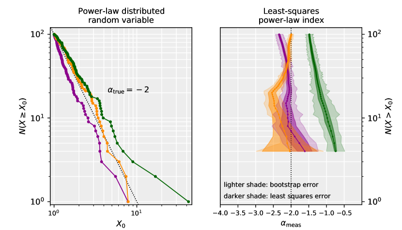
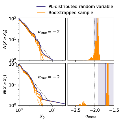
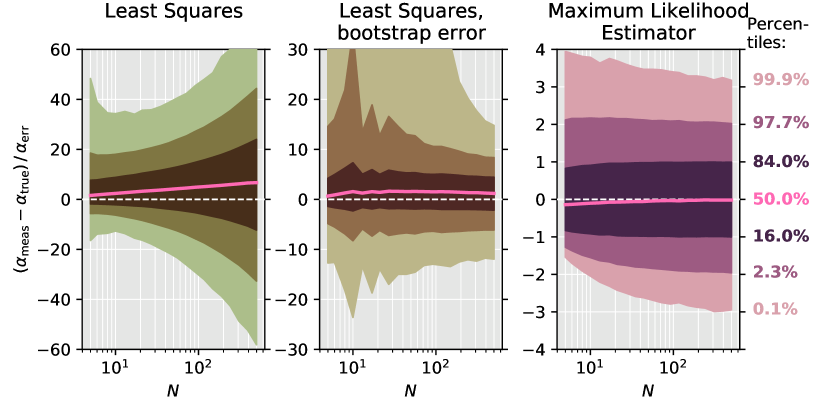
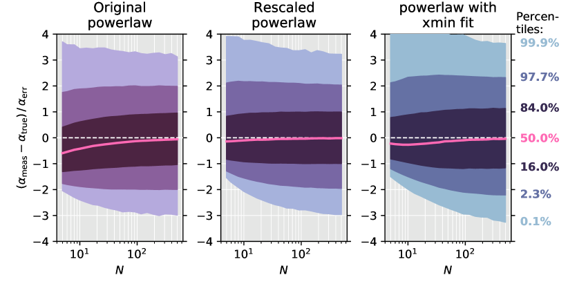
In this section we will investigate accuracy and bias of PLI estimates provided by the graphical and MLE methods. We start with demonstrating the sub-optimal performance of the least squares estimates. To do this, we generated three realizations of PL-distributed random variables using a Pareto distribution from the python library scipy, with survival function defined as:
| (10) |
We took , , and . PLIs were estimated using graphical method on the unbinned survival functions. In order to investigate the dependence of the PLI produced by the graphical method on the sample size, we performed fits on reduced samples, selecting , where ranged from the smallest to the fourth largest values of . For each fit both the least-squares and bootstrapping errors were estimated. For the latter we followed the procedure from Kirsten et al. (2024), removing 10% of the sample without replacement (or one element if ), calculating the PLI, repeating this 100 times and then taking standard deviation of the acquired distribution as , the error on . Figure 20 displays the survival functions and the resulting . Even for , the resulting PLI can deviate from the true value by as much as 25%, while the formal errors are an order of magnitude smaller.
The uncertainties in PLI measurements calculated using the bootstrapping method are indicative at best. The distribution of on bootstrapped sub-samples is generally skewed towards shallower PLIs (Fig. 21). The shape of the SF tail can be heavily influenced by a few large random variables, which constitute a small fraction of the entire sample. Depending on the chance presence of these variables in the bootstrapped sub-sample, the measured PLI can vary substantially, resulting in multimodal bootstrapped PLI distributions (Fig. 21, lower row). This has a significant effect on the calculated standard deviation of bootstrapped PLIs, causing large scatter in the bootstrapped error on from one simulation to another. At the same time, the error is not large enough to describe the true discrepancy between and (Fig. 20).
To further test the quality of the PL fitting, we examined the distributions of test statistics , for several fitting methods. We generated a series of samples with ranging from 5 to 500, values for and . Performing smaller tests using different values of did not reveal any differences in the behavior of examined distributions.
Fig. 22 shows the accuracy of the fit for three methods: graphical with its standard errors, graphical with the bootstrap errors, and MLE (where we emphasize here that the 3 relevant ordinates in that Figure are on different scales). Following James et al. (2019), we used unbiased estimates:
| (11) |
For we used the expression from the same work, despite it being valid only for large :
| (12) |
In the ideal case follows a normal distribution with a median of 0 and a standard deviation . This means that provides an unbiased estimate of , and has an intuitive Gaussian meaning. To illustrate how closely obeys a normal distribution we plot, in Fig. 22 (right sub-panel) , the percentiles at levels corresponding to the median and its , , and counterparts. For the MLE method and relatively large sample sizes , these levels are at , indicating that very closely resembles the normal distribution. For smaller sample sizes is skewed towards negative values, and accurately described by a gamma distribution (Eq. 2). We note that the median value of stays close to 0 for all sample sizes.
In stark contrast to this, the graphical method leads to a median value of on the order of 5 for the least squares error and 1.5 for the bootstrap error, indicating that median tends to be larger than by a few , regardless of sample size. The wide spread of the percentile curves in Fig. 22 (left and middle sub-panel) demonstrates that values are substantially underestimated when choosing to use the graphical method .
We performed similar accuracy estimates for PLIs determined with the python package powerlaw202020https://pypi.org/project/powerlaw/ (Alstott et al., 2014). In the original code, and are calculated as
| (13) |
and
| (14) |
Fig. 23 (left panel) shows that this estimate performs worse than the version modified according to Eqs. 11-12 (center panel).
In real-life observations is often not known. The powerlaw package offers fitting for the best by minimizing the Kolmogorov-Smirnov distance between the data and the theoretical power-law fit. We have repeated the aforementioned simulations with fitting for , restricting its range from to the third largest value. In this case, the median value of is slightly more biased towards small negative values and the distribution is somewhat wider (Fig. 23), but the MLE still provides a much better fit than the graphical method.
References
- Adams & van Leeuwen (2019) Adams, E. A. K. & van Leeuwen, J. 2019, Nature Astronomy, 3, 188
- Alstott et al. (2014) Alstott, J., Bullmore, E., & Plenz, D. 2014, PLoS ONE 9, e85777
- Atri et al. (2022) Atri, P., Bilous, A., van Leeuwen, J., et al. 2022, The Astronomer’s Telegram, 15197, 1
- Beniamini et al. (2020) Beniamini, P., Wadiasingh, Z., & Metzger, B. D. 2020, MNRAS, 496, 3390
- Bethapudi et al. (2023) Bethapudi, S., Spitler, L. G., Main, R. A., Li, D. Z., & Wharton, R. S. 2023, MNRAS, 524, 3303
- Bilous et al. (2022) Bilous, A. V., Grießmeier, J. M., Pennucci, T., et al. 2022, A&A, 658, A143
- Caleb et al. (2022) Caleb, M., Heywood, I., Rajwade, K., et al. 2022, Nature Astronomy, 6, 828
- Chen et al. (2024) Chen, X., Hu, B., Wang, P., et al. 2024, arXiv e-prints, arXiv:2401.18036
- CHIME/FRB et al. (2020) CHIME/FRB, Amiri, M., Andersen, B. C., et al. 2020, Nature, 582, 351
- CHIME/FRB Collaboration et al. (2021) CHIME/FRB Collaboration, Amiri, M., Andersen, B. C., et al. 2021, ApJS, 257, 59
- Chime/FRB Collaboration et al. (2022) Chime/FRB Collaboration, Andersen, B. C., Bandura, K., Bhardwaj, M., et al. 2022, Nature, 607, 256
- Connor & van Leeuwen (2018) Connor, L. & van Leeuwen, J. 2018, AJ, 156, 256
- Connor et al. (2020) Connor, L., van Leeuwen, J., Oostrum, L. C., et al. 2020, MNRAS, 499, 4716
- Cordes (1978) Cordes, J. M. 1978, ApJ, 222, 1006
- Cui et al. (2021) Cui, X.-H., Zhang, C.-M., Wang, S.-Q., et al. 2021, Research in Astronomy and Astrophysics, 21, 211
- Du et al. (2023) Du, C., Huang, Y.-F., Zhang, Z.-B., et al. 2023, arXiv e-prints, arXiv:2310.08971
- Gardenier et al. (2019) Gardenier, D. W., van Leeuwen, J., Connor, L., & Petroff, E. 2019, A&A, 632, A125
- Goldstein et al. (2004) Goldstein, M., Morris, S., & Yen, G. 2004, The European Physical Journal B - Condensed Matter and Complex Systems, 41, 255
- Gupta et al. (2017) Gupta, Y., Ajithkumar, B., Kale, H. S., et al. 2017, Current Science, 113, 707
- Hilmarsson et al. (2021) Hilmarsson, G. H., Spitler, L. G., Main, R. A., & Li, D. Z. 2021, MNRAS, 508, 5354
- Hoogenboom et al. (2006) Hoogenboom, J. P., den Otter, W. K., & Offerhaus, H. L. 2006, The Journal of Chemical Physics, 125, 204713
- James et al. (2019) James, C. W., Ekers, R. D., Macquart, J. P., Bannister, K. W., & Shannon, R. M. 2019, MNRAS, 483, 1342
- Jiang et al. (2022) Jiang, J.-C., Wang, W.-Y., Xu, H., et al. 2022, Research in Astronomy and Astrophysics, 22, 124003
- Johnston et al. (2023) Johnston, S., Kramer, M., Karastergiou, A., et al. 2023, MNRAS, 520, 4801
- Johnston et al. (2024) Johnston, S., Mitra, D., Keith, M. J., Oswald, L. S., & Karastergiou, A. 2024, MNRAS, 530, 4839
- Kirsten et al. (2024) Kirsten, F., Ould-Boukattine, O. S., Herrmann, W., et al. 2024, Nature Astronomy, 8, 337
- Kramer et al. (2007) Kramer, M., Stappers, B., Jessner, A., Lyne, A., & Jordan, C. 2007, Monthly Notices of the Royal Astronomical Society, 377, 107
- Kumar et al. (2022) Kumar, P., Shannon, R. M., Lower, M. E., et al. 2022, MNRAS, 512, 3400
- Lanman et al. (2022) Lanman, A. E., Andersen, B. C., Chawla, P., et al. 2022, ApJ, 927, 59
- Lorimer et al. (2007) Lorimer, D. R., Bailes, M., McLaughlin, M. A., Narkevic, D. J., & Crawford, F. 2007, Science, 318, 777
- Lorimer & Kramer (2005) Lorimer, D. R. & Kramer, M. 2005, Handbook of Pulsar Astronomy (Cambridge University Press)
- Lu et al. (2023) Lu, W.-J., Zhao, Z.-Y., Wang, F. Y., & Dai, Z. G. 2023, ApJ, 956, L9
- Lyutikov (2016) Lyutikov, M. 2016, arXiv e-prints, arXiv:1607.00777
- Lyutikov (2020) Lyutikov, M. 2020, ApJ, 889, 135
- Maan & van Leeuwen (2017) Maan, Y. & van Leeuwen, J. 2017, IEEE Proc. URSI GASS
- Maan et al. (2021) Maan, Y., van Leeuwen, J., & Vohl, D. 2021, A&A, 650, A80
- Main et al. (2021) Main, R., Bethapudi, S., & Marthi, V. 2021, The Astronomer’s Telegram, 14933, 1
- Main et al. (2022) Main, R. A., Hilmarsson, G. H., Marthi, V. R., et al. 2022, MNRAS, 509, 3172
- Mao et al. (2022) Mao, J.-W., Yuan, J.-P., Wen, Z.-G., et al. 2022, Research in Astronomy and Astrophysics, 22, 065006
- Marthi et al. (2022) Marthi, V. R., Bethapudi, S., Main, R. A., et al. 2022, MNRAS, 509, 2209
- Men & Barr (2024) Men, Y. & Barr, E. 2024, A&A, 683, A183
- Metzger et al. (2017) Metzger, B. D., Berger, E., & Margalit, B. 2017, ApJ, 841, 14
- Mitra et al. (2015) Mitra, D., Arjunwadkar, M., & Rankin, J. M. 2015, ApJ, 806, 236
- Mitra et al. (2016) Mitra, D., Basu, R., Maciesiak, K., et al. 2016, ApJ, 833, 28
- Morello et al. (2022) Morello, V., Rajwade, K. M., & Stappers, B. W. 2022, MNRAS, 510, 1393
- Nimmo et al. (2022) Nimmo, K., Hewitt, D. M., Hessels, J. W. T., et al. 2022, ApJ, 927, L3
- Niu et al. (2022) Niu, J.-R., Zhu, W.-W., Zhang, B., et al. 2022, Research in Astronomy and Astrophysics, 22, 124004
- Oostrum (2021) Oostrum, L. 2021, DARC: Data Analysis of Real-time Candidates, 10.5281/zenodo.3784870
- Oostrum et al. (2020) Oostrum, L. C., Maan, Y., van Leeuwen, J., et al. 2020, A&A, 635, A61
- Oostrum (2020) Oostrum, L. C. L. 2020, PhD thesis, University of Amsterdam, Netherlands
- Ould-Boukattine et al. (2024) Ould-Boukattine, O. S., Dijkema, T. J., Gawronski, M., et al. 2024, The Astronomer’s Telegram, 16565, 1
- Ould-Boukattine et al. (2022) Ould-Boukattine, O. S., Kirsten, F., Nimmo, K., et al. 2022, The Astronomer’s Telegram, 15190, 1
- Pastor-Marazuela et al. (2021) Pastor-Marazuela, I., Connor, L., van Leeuwen, J., et al. 2021, Nature, 596, 505
- Pastor-Marazuela et al. (2023) Pastor-Marazuela, I., van Leeuwen, J., Bilous, A., et al. 2023, A&A, 678, A149
- Pastor-Marazuela et al. (2024) Pastor-Marazuela, I., van Leeuwen, J., Bilous, A., et al. 2024, arXiv e-prints, arXiv:2406.00482
- Perley & Butler (2017) Perley, R. A. & Butler, B. J. 2017, ApJS, 230, 7
- Petroff et al. (2019) Petroff, E., Hessels, J. W. T., & Lorimer, D. R. 2019, A&A Rev., 27, 4
- Petroff et al. (2022) Petroff, E., Hessels, J. W. T., & Lorimer, D. R. 2022, A&A Rev., 30, 2
- Philippov et al. (2020) Philippov, A., Timokhin, A., & Spitkovsky, A. 2020, Phys. Rev. Lett., 124, 245101
- Platts et al. (2021) Platts, E., Caleb, M., Stappers, B. W., et al. 2021, MNRAS, 505, 3041
- Platts et al. (2019) Platts, E., Weltman, A., Walters, A., et al. 2019, Phys. Rep, 821, 1
- Pleunis et al. (2021a) Pleunis, Z., Good, D. C., Kaspi, V. M., et al. 2021a, ApJ, 923, 1
- Pleunis et al. (2021b) Pleunis, Z., Michilli, D., Bassa, C. G., et al. 2021b, ApJ, 911, L3
- Popov & Stappers (2007) Popov, M. V. & Stappers, B. 2007, A&A, 470, 1003
- Radhakrishnan & Cooke (1969) Radhakrishnan, V. & Cooke, D. J. 1969, Astrophys. Lett., 3, 225
- Ransom et al. (2002) Ransom, S. M., Eikenberry, S. S., & Middleditch, J. 2002, AJ, 124, 1788
- Roy et al. (2018) Roy, J., Chengalur, J. N., & Pen, U.-L. 2018, ApJ, 864, 160
- Sang & Lin (2023) Sang, Y. & Lin, H.-N. 2023, MNRAS
- Sclocco et al. (2016) Sclocco, A., van Leeuwen, J., Bal, H. E., & van Nieuwpoort, R. V. 2016, Astronomy and Computing, 14, 1
- Seymour et al. (2019) Seymour, A., Michilli, D., & Pleunis, Z. 2019, DM_phase: Algorithm for correcting dispersion of radio signals, Astrophysics Source Code Library, record ascl:1910.004
- Sobacchi et al. (2023) Sobacchi, E., Lyubarsky, Y., Beloborodov, A. M., Sironi, L., & Iwamoto, M. 2023, ApJ, 943, L21
- Takefuji et al. (2022) Takefuji, K., Murata, Y., Ikebe, S., et al. 2022, The Astronomer’s Telegram, 15285, 1
- Totani & Tsuzuki (2023) Totani, T. & Tsuzuki, Y. 2023, MNRAS, 526, 2795
- Trudu et al. (2022) Trudu, M., Pilia, M., Bernardi, G., et al. 2022, MNRAS, 513, 1858
- Tsuzuki et al. (2024) Tsuzuki, Y., Totani, T., Hu, C.-P., & Enoto, T. 2024, MNRAS, 530, 1885
- van Cappellen et al. (2022) van Cappellen, W. A., Oosterloo, T. A., Verheijen, M. A. W., et al. 2022, A&A, 658, A146
- van Leeuwen (2014) van Leeuwen, J. 2014, in ”The Third Hot-wiring the Transient Universe Workshop”, ed. P. R. Wozniak, M. J. Graham, A. A. Mahabal, & R. Seaman, 79
- van Leeuwen et al. (2023) van Leeuwen, J., Kooistra, E., Oostrum, L., et al. 2023, A&A, 672, A117
- Wadiasingh et al. (2020) Wadiasingh, Z., Beniamini, P., Timokhin, A., et al. 2020, ApJ, 891, 82
- Wadiasingh & Chirenti (2020) Wadiasingh, Z. & Chirenti, C. 2020, ApJ, 903, L38
- Wadiasingh & Timokhin (2019) Wadiasingh, Z. & Timokhin, A. 2019, ApJ, 879, 4
- Wang et al. (2023a) Wang, B.-J., Xu, H., Jiang, J.-C., et al. 2023a, Chinese Physics B, 32, 029801
- Wang et al. (2019) Wang, W., Zhang, B., Chen, X., & Xu, R. 2019, ApJ, 876, L15
- Wang & van Leeuwen (2024) Wang, Y. & van Leeuwen, J. 2024, arXiv e-prints, arXiv:2405.06281
- Wang et al. (2023b) Wang, Y.-B., Kurban, A., Zhou, X., Yu, Y.-W., & Wang, N. 2023b, MNRAS, 524, 569
- Wu et al. (2024) Wu, Z., Zhu, W., Zhang, B., et al. 2024, arXiv e-prints, arXiv:2406.12218
- Xiao et al. (2024) Xiao, D., Dai, Z.-G., & Wu, X.-F. 2024, ApJ, 962, 35
- Xu et al. (2022) Xu, H., Niu, J. R., Chen, P., et al. 2022, Nature, 609, 685
- Zhang et al. (2022) Zhang, Y.-K., Wang, P., Feng, Y., et al. 2022, Research in Astronomy and Astrophysics, 22, 124002
- Zhou et al. (2022) Zhou, D. J., Han, J. L., Zhang, B., et al. 2022, Research in Astronomy and Astrophysics, 22, 124001