Differentially Private Convex Approximation of
Two-Layer ReLU Networks

Abstract

We show that it is possible to privately train convex problems that give models with similar privacy-utility trade-off as one hidden-layer ReLU networks trained with differentially private stochastic gradient descent (DP-SGD). As we show, this is possible via a certain dual formulation of the ReLU minimization problem. We derive a stochastic approximation of the dual problem that leads to a strongly convex problem which allows applying, for example, the privacy amplification by iteration type of analysis for gradient-based private optimizers, and in particular allows giving accurate privacy bounds for the noisy cyclic mini-batch gradient descent with fixed disjoint mini-batches. We obtain on the MNIST and FashionMNIST problems for the noisy cyclic mini-batch gradient descent first empirical results that show similar privacy-utility-trade-offs as DP-SGD applied to a ReLU network. We outline theoretical utility bounds that illustrate the speed-ups of the private convex approximation of ReLU networks.

1 Introduction

In differentially private (DP) machine learning (ML), the DP-SGD algorithm (see e.g., Abadi et al., 2016a, ) has become a standard tool obtain ML models with strong privacy guarantees of the individuals. In DP-SGD, the $(\varepsilon,\delta)$-guarantees for the ML model are obtained by clipping gradients to have a bounded Euclidean norm and by adding normally distributed noise scaled with the clipping constant to the mini-batch gradients.

One weak point of the privacy analysis of DP-SGD is that it is assumes that the adversary has access to all the intermediate results of the training iteration. This assumption is unnecessarily strict as often only the final model is needed. As a result, the $(\varepsilon,\delta)$-guarantees are possibly pessimistic when compared to the performance of even the most effective computational attacks (Nasr et al.,, 2021). Another weakness is that the formal guarantees require either full batch training or random subsampling, and, e.g., accurate privacy analyses of many practically relevant algorithms such as noisy cyclic mini-batch GD are not available for non-convex problems such as multi-layer neural networks.

The challenges are how to find realistic $(\varepsilon,\delta)$-guarantees that hold only for the final model and how to analyse practical algorithms such as the noisy cyclic mini-batch GD for problems that give high-utility models. With the former, the hope is that less DP noise would be needed and higher-accuracy DP ML models would be obtained and with the latter, that efficient large-scale implementations would be possible for high-utility models (Chua et al.,, 2024).

To reach these goals, we either have to come up with new privacy accounting techniques that are applicable for general non-convex problems, or then, alternatively, simplify the problems so that they are amenable to existing DP analyses for convex problems. When considering releasing only the final model, existing $(\varepsilon,\delta)$-DP analyses in the literature are applicable for convex problems (such as the logistic regression) and for strongly convex problems (such the logistic regression with $L_{2}$-regularization). When training models with DP-SGD, one quickly finds that the model performance of commonly used convex models is inferior compared to multi-layer neural networks. A natural question arises: can we somehow make convex approximations of minimization problems for multi-layer neural networks that would retain the performance of the models we obtain from the non-convex problems? As a first step to answer this question, we consider in this work such an approximation of the 2-layer ReLU minimization problem.

1.1 Further Motivation for Convex Approximation and Related Literature

In private DP-SGD based optimization clipping of the gradients and the added noise complicate the optimization (Chen et al.,, 2020) which is also reflected in theoretical utility bounds which are difficult to obtain in the non-convex setting. State-of-the-art Empirical Risk Minimization (ERM) bounds for private convex optimization are of the order $O(\tfrac{1}{\sqrt{n}}+\tfrac{\sqrt{d}}{\varepsilon n})$, where $n$ is the number of training data entries, $d$ the dimension of the parameter space and $\varepsilon$ the DP parameter (Bassily et al.,, 2019). Corresponding upper bounds in case of non-convex optimization are of the order $O(\frac{1}{n^{1/3}}+\frac{d^{1/5}}{(\varepsilon n)^{2/5}})$ (Bassily et al.,, 2021). Thus, also from the theoretical perspective, DP training of convex models is favorable over non-convex ones. In order to approximate a two-layer ReLU network which can already considerably improve the model performance upon convex problems such as the logistic regression, we use the results of Pilanci and Ergen, (2020) that show that there exist a certain convex dual formulation for the 2-layer ReLU minimization problem in case the hidden-layer of the ReLU network is sufficiently wide. We also remark that these kind of equivalent convex formulations have also be shown for 2-layer convolutional networks (Bartan and Pilanci,, 2019) and for multi-layer ReLU networks (Ergen and Pilanci,, 2021).

The so-called privacy amplification by iteration analysis for convex private optimization leads to privacy guarantees for the final model and was initiated by Feldman et al., (2018). Their analysis and many subsequent ones (Sordello et al.,, 2021; Asoodeh et al.,, 2020; Balle et al.,, 2019) are still difficult to apply in practice in a sense that it commonly takes very large number of training iterations before one gets DP guarantees that are tighter that those of DP-SGD and as a result it is also difficult to obtain models with better privacy-utility trade-offs than by using DP-SGD. Chourasia et al., (2021) have given an improved analysis for the full batch DP-GD training and Ye and Shokri, (2022) have also given a similar analysis for the shuffled mini-batch DP-SGD. The analysis has been recently further tightened by Bok et al., (2024) whose results we use to analyse the noisy cyclic mini-batch GD.

2 Preliminaries

We denote a dataset containing $n$ data points as $D=(z_{1},\ldots,z_{n}).$ We say $D$ and $D^{\prime}$ are neighboring datasets if they differ in exactly one element (denoted as $D\sim D^{\prime}$). We say that a mechanism $\mathcal{M}\,:\,\mathcal{X}\rightarrow\mathcal{O}$ is $(\varepsilon,\delta)$-DP if the output distributions for neighboring datasets are always $(\varepsilon,\delta)$-indistinguishable (Dwork et al.,, 2006).

Definition 1.

Let $\varepsilon\geq 0$ and $\delta\in[0,1]$. Mechanism $\mathcal{M}\,:\,\mathcal{X}\rightarrow\mathcal{O}$ is $(\varepsilon,\delta)$-DP if for every pair of neighboring datasets $D,D^{\prime}$ and for every measurable set $E\subset\mathcal{O}$,

$$\mathbb{P}(\mathcal{M}(D)\in E)\leq{\rm e}\hskip 1.0pt^{\varepsilon}\mathbb{P}(\mathcal{M}(D^{\prime})\in E)+\delta.$$

We call $\mathcal{M}$ tightly $(\varepsilon,\delta)$-DP, if there does not exist $\delta^{\prime}<\delta$ such that $\mathcal{M}$ is $(\varepsilon,\delta^{\prime})$-DP.

Hockey-stick Divergence and Numerical Privacy Accounting.

The DP guarantees can be alternatively described using the hockey-stick divergence which is defined as follows. For $\alpha>0$ the hockey-stick divergence $H_{\alpha}$ from a distribution $P$ to a distribution $Q$ is defined as

$$H_{\alpha}(P||Q)=\int\left[P(t)-\alpha\cdot Q(t)\right]_{+}\,\hskip 1.0pt{\rm d}\hskip 0.5ptt,$$ (2.1)

where for $t\in\mathbb{R}$, $[t]_{+}=\max\{0,t\}$. The $(\varepsilon,\delta)$-DP guarantee as defined in Def. 1 can be characterized using the hockey-stick divergence as follows.

Lemma 2 (Zhu et al., 2022).

For a given $\varepsilon\geq 0$, tight $\delta(\varepsilon)$ is given by the expression

$$\delta(\varepsilon)=\max_{D\sim D^{\prime}}H_{{\rm e}\hskip 1.0pt^{\varepsilon}}(\mathcal{M}(D)||\mathcal{M}(D^{\prime})).$$

Thus, if we can bound the divergence $H_{{\rm e}\hskip 1.0pt^{\varepsilon}}(\mathcal{M}(D)||\mathcal{M}(D^{\prime}))$ accurately, we also obtain accurate $\delta(\varepsilon)$-bounds. where To this end we need to consider so-called dominating pairs of distributions.

Definition 3 (Zhu et al., 2022).

A pair of distributions $(P,Q)$ is a dominating pair of distributions for mechanism $\mathcal{M}(D)$ if for all neighboring datasets $D$ and $D^{\prime}$ and for all $\alpha>0$,

$$H_{\alpha}(\mathcal{M}(D)||\mathcal{M}(D^{\prime}))\leq H_{\alpha}(P||Q).$$

If the equality holds for all $\alpha$ for some $D,D^{\prime}$, then $(P,Q)$ is a tightly dominating pair of distributions.

We get upper bounds for DP-SGD compositions using the dominating pairs of distributions using the following composition result.

Theorem 4 (Zhu et al., 2022).

If $(P,Q)$ dominates $\mathcal{M}$ and $(P^{\prime},Q^{\prime})$ dominates $\mathcal{M}^{\prime}$, then $(P\times P^{\prime},Q\times Q^{\prime})$ dominates the adaptive composition $\mathcal{M}\circ\mathcal{M}^{\prime}$.

To convert the hockey-stick divergence from $P\times P^{\prime}$ to $Q\times Q^{\prime}$ into an efficiently computable form, we consider so called privacy loss random variables (PRVs) and use Fast Fourier Technique-based methods (Koskela et al.,, 2021; Gopi et al.,, 2021) to numerically evaluate the convolutions appearing when summing the PRVs and evaluating $\delta(\varepsilon)$ for the compositions.

Gaussian Differential Privacy.

For the privacy accounting of the noisy cyclic mini-batch GD, we use the bounds by Bok et al., (2024) that are stated using the Gaussian differential privacy (GDP). Informally speaking, a mechanism $\mathcal{M}$ is $\mu$-GDP, $\mu\geq 0$, if for all neighboring datasets the outcomes of $\mathcal{M}$ are not more distinguishable than two unit-variance Gaussians $\mu$ apart from each other (Dong et al.,, 2022). We consider the following formal characterization of GDP.

Lemma 5 (Dong et al., 2022, Cor. 2.13).

A mechanism $\mathcal{M}$ is $\mu$-GDP if and only it is $(\varepsilon,\delta)$-DP for all $\varepsilon\geq 0$, where

$$\delta(\varepsilon)=\Phi\left(-\frac{\varepsilon}{\mu}+\frac{\mu}{2}\right)-{\rm e}\hskip 1.0pt^{\varepsilon}\Phi\left(-\frac{\varepsilon}{\mu}-\frac{\mu}{2}\right).$$

2.1 DP-SGD with Subsampling Without Replacement

We want to experimentally compare DP-SGD to the noisy cyclic mini-batch gradient descent using the privacy amplification by iteration analysis Bok et al., (2024). To this end, we consider the substitute neighborhood relation of datasets and thus cannot use the commonly considered Poisson subsampling amplification results for DP-SGD that hold for the add/remove neighborhood relation of datasets. Instead, we rely on the results by Zhu et al., (2022) and consider DP-SGD with subsampling without replacement of fixed-sized mini-batches, for which one iteration is given by

$$\theta_{j+1}=\theta_{j}-\eta_{j}\cdot\Big{(}\frac{1}{b}\sum\nolimits_{x\in B_{j}}\text{clip}(\nabla\mathcal{L}(x,\theta_{j}),C)+Z_{j}\Big{)},$$ (2.2)

where $C>0$ denotes the clipping constant, $\text{clip}(\cdot,C)$ the clipping function that clips gradients to have 2-norm at most $C$, $\mathcal{L}$ the loss function, $\theta$ the model parameters, $\eta_{j}$ the learning rate at iteration $j$, $B_{j}$ the mini-batch at iteration $j$ that is sampled without replacement, $b$ the size of each mini-batch and $Z_{j}\sim\mathcal{N}(0,\tfrac{C^{2}\sigma^{2}}{b^{2}}I_{d})$ the noise vector.

This also means that we cannot use the numerical accounting methods designed for the Poisson subsampling under the add/remove neighborhood relation (Gopi et al.,, 2021; Zhu et al.,, 2022). We consider a numerical approach also used in Koskela et al., (Sec. 3.4 2023). We use the following subsampling amplification result, which leads to a privacy profile for the composed mechanism $\mathcal{M}\circ S_{Subset}$, where $S_{Subset}$ denotes a subsampling procedure where, from an input of $n$ entries, a fixed sized subset of $q\cdot n$, $0<q\leq 1$, entries is sampled without replacement.

Lemma 6 (Zhu et al., 2022).

Denote the subsampled mechanism $\widetilde{\mathcal{M}}:=\mathcal{M}\circ S_{Subset}$. Suppose a pair of distributions $(P,Q)$ is a dominating pair of distributions for a mechanism $\mathcal{M}$ for all datasets of size $q\cdot n$ under the $\sim$-neighbouring relation (i.e., the substitute relation), where $q>0$ is the subsampling ratio (size of the subset divided by $n$). Then, for all neighbouring datasets (under the $\sim$-neighbouring relation) $X$ and $Y$ of size $n$,

$$H_{\alpha}\big{(}\widetilde{\mathcal{M}}(X)||\widetilde{\mathcal{M}}(Y)\big{)} \leq H_{\alpha}\big{(}q\cdot P+(1-q)\cdot Q||Q\big{)},\quad\textrm{for }\alpha\geq 1,$$ (2.3)

$$H_{\alpha}\big{(}\widetilde{\mathcal{M}}(X)||\widetilde{\mathcal{M}}(Y)\big{)} \leq H_{\alpha}\big{(}P||q\cdot Q+(1-q)\cdot P\big{)},\quad\textrm{for }0\leq\alpha<1.$$

We can describe the upper bound given by Lemma 6 by a function $h\,:\,\mathbb{R}_{\geq 0}\rightarrow\mathbb{R}$ defined as

$$h(\alpha)=\max\{H_{\alpha}\big{(}q\cdot P+(1-q)\cdot Q||Q\big{)},H_{\alpha}\big{(}P||q\cdot Q+(1-q)\cdot P\big{)}\}.$$ (2.4)

We see that $h(\alpha)$ defines a privacy profile: as a maximum of convex functions it is convex and has all other required properties of a privacy profile (Doroshenko et al.,, 2022). Thus we can use an existing numerical method (Doroshenko et al.,, 2022, Algorithm 1) with the privacy profile $h$ to obtain discrete-valued distributions $\widetilde{P}$ and $\widetilde{Q}$, that give a dominating pair for the subsampled mechanism $\mathcal{M}\circ S_{Subset}$. Furthermore, using the composition result of Lemma 4 and numerical accountants, we obtain $(\varepsilon,\delta)$-bounds for compositions of DP-SGD with subsampling without replacement. Alternatively, we could use RDP bounds given by Wang et al., (2019), however, as also illustrated by the Appendix Figure 6, our numerical approach generally leads to tighter bounds.

2.2 Guarantees for the Final Model and for Noisy Cyclic Mini-Batch GD

We next consider privacy amplification by iteration (Feldman et al.,, 2018) type of analysis that gives DP guarantees for the final model of the training iteration. We use the recent results by Bok et al., (2024) that are applicable to the noisy cyclic mini-batch gradient descent (NoisyCGD) for which one epoch of training is described by the iteration

$$\theta_{j+1}=\theta_{j}-\eta\left(\frac{1}{b}\sum\nolimits_{x\in B_{j}}\nabla_{\theta}f(\theta_{j},x)+Z_{j}\right)$$ (2.5)

where $Z_{j}\sim\mathcal{N}(0,\sigma^{2}I_{d})$ and the data $D$, $\left|D\right|=n$, is divided into disjoint batches $B_{1},\ldots,B_{k}$, each of size $b$. The analysis by Bok et al., (2024) considers the substitute neighborhood relation of datasets and central for the DP analysis is the gradient sensitivity.

Definition 7.

We say that a family of loss functions $\mathcal{F}$ has a gradient sensitivity $L$ if

$$\sup_{f,g\in\mathcal{F}}\left\lVert\nabla f-\nabla g\right\rVert\leq L.$$

As an example relevant to our analysis, for a family of loss functions of the form $h_{i}+r$, where $h_{i}$’s are $L$-Lipschitz loss functions and $r$ is a regularization function, the sensitivity equals $2L$. We will use the following result for analysing the $(\varepsilon,\delta)$-DP guarantees of NoisyCGD. First, recall that a function $f$ is $\beta$-smooth if $\nabla f$ is $\beta$-Lipschitz, and it is $\lambda$-strongly convex if the function $g(x)=f(x)-\frac{\lambda}{2}\left\lVert x\right\rVert_{2}^{2}$ is convex.

Theorem 8 (Bok et al., 2024, Thm. 4.5).

Consider $\lambda$-strongly convex, $\beta$-smooth loss functions with gradient sensitivity $L$. Then, for any $\eta\in(0,2/M)$, NoisyCGD is $\mu$-GDP for

$$\mu=\frac{L}{b\sigma}\sqrt{1+c^{2k-2}\frac{1-c^{2}}{(1-c^{k})^{2}}\frac{1-c^{k(E-1)}}{1+c^{k(E-1)}}},$$

where $k=n/b$, $c=\max\{\left|1-\eta\lambda\right|,\left|1-\eta\beta\right|\}$ and $E$ denotes the number of epochs.

We could alternatively use the RDP analysis by Ye and Shokri, (2022), however, as also illustrated by the experiments of Bok et al., (2024), the bounds given by Thm. 8 lead to slightly lower $(\varepsilon,\delta)$-DP bounds for NoisyCGD.

In order to benefit from the privacy analysis of Thm. 8 for NoisyCGD, we add an $L_{2}$-regularization term with a coefficient $\tfrac{\lambda}{2}$ which makes the loss function $\lambda$-strongly convex. Finding suitable values for the learning rate $\eta$ and regularization parameter $\lambda$ is complicated by the following aspects. The larger the regularization parameter $\lambda$ and the learning rate $\eta$ are, the faster the model ’forgets’ the past updates and the faster the $\varepsilon$-values converge. This is reflected in the GDP bound of Thm.  8 in the constant $c$ which generally equals $\left|1-\eta\lambda\right|$. Thus, in order to benefit from the bound of Thm.  8, the product $\eta\lambda$ should not be too small. On the other hand, when $\eta\lambda$ is too large, the ’forgetting’ starts to affect the model performance. We experimentally observe that the plateauing of the model accuracy and privacy guarantees happens approximately at the same time.

In order to simplify the experimental comparisons which we present in Section 5, we train all models for 400 epochs, each with batch size 1000. Figure 1 illustrates a range of values for the product $\eta\lambda$ where the $(\varepsilon,\delta)$-guarantees given by Thm.  8 become smaller than those given by the DP-SGD analysis with an equal batch size when $\sigma=15.0$. Among the values depicted in Fig. 1, $\eta\lambda=4\cdot 10^{-4}$ is experimentally found to already affect the model performance considerably whereas $\eta\lambda=2\cdot 10^{-4}$ affects only weakly. Thus, in order to simplify the experiments, we make the decision that when tuning the learning rate hyperparameter we set $\lambda$ such that $\eta\lambda=2\cdot 10^{-4}$.

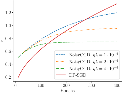
Figure 1: Values of the product of the learning rate $\eta$ and the $L_{2}$-regularization constant $\lambda$ that lead to tighter privacy bounds for the final model using Thm. 8 than for the whole sequence of updates using the DP-SGD analysis. Here the $\varepsilon$-values are shown as a function of number of training epochs, when total number of training samples $N=6\cdot 10^{4}$, the batch size $b=1000$, $\sigma=15.0$ and $\delta=10^{-5}$. We search for a hyperparameter combination ($\eta,\lambda$) that at the same time preserves the learning capacity of the convexified model and gives smaller $\varepsilon$-values for NoisyCGD.

3 Convex Approximation of Two-Layer ReLU Networks

We next derive step by step the strongly convex approximation of the 2-layer ReLU minimization problem and show that the derived problem is amenable for the privacy amplification by iteration type of $(\varepsilon,\delta)$-DP analysis. To simplify the presentation, we consider a 1-dimensional output network (e.g., a binary classifier). It will be straightforward to construct multivariate output networks from the scalar networks (see also Ergen et al.,, 2023).

3.1 Convex Duality of Two-layer ReLU Problem

We first consider the convex reformulation of the 2-layer ReLU minimization problem as presented by Pilanci and Ergen (2020). In particular, consider training a 2-layer ReLU network (with hidden-width $m$) $f\,:\,\mathbb{R}^{d}\rightarrow\mathbb{R}$,

$$f(x)=\sum\nolimits_{j=1}^{m}\phi(u_{j}^{T}x)\alpha_{j},$$ (3.1)

where the weights $u_{i}\in\mathbb{R}^{d}$, $i\in[m]$ and $\alpha\in\mathbb{R}^{m}$, and $\phi$ is the ReLU activation function, i.e., $\phi(t)=\max\{0,t\}$. For a vector $x$, $\phi$ is applied element-wise, i.e. $\phi(x)_{i}=\phi(x_{i})$.

Using the squared loss and $L_{2}$-regularization with a regularization constant $\lambda>0$, the 2-layer ReLU minimization problem can then be written as

$$\min_{\{u_{i},\alpha_{i}\}_{i=1}^{m}}\frac{1}{2}\left\lVert\sum\nolimits_{i=1}^{m}\phi(Xu_{i})\alpha_{i}-y\right\rVert_{2}^{2}+\frac{\lambda}{2}\sum\limits_{i=1}^{m}(\left\lVert u_{i}\right\rVert_{2}^{2}+\alpha_{i}^{2}),$$ (3.2)

where $X\in\mathbb{R}^{n\times d}$ denotes the matrix of the feature vectors, i.e., $X^{T}=\begin{bmatrix}x_{1}&\ldots&x_{n}\end{bmatrix}$ and $y\in\mathbb{R}^{n}$ denotes the vector of labels.

The convex reformulation of this problem is based on enumerating all the possible activation patterns of $\phi(Xu)$, $u\in\mathbb{R}^{d}$. The set of activation patterns that a ReLU output $\phi(Xu)$ can take for a data feature matrix $X\in\mathbb{R}^{n\times d}$ is described by the set of diagonal boolean matrices

$$\mathcal{D}_{X}=\{D=\mathrm{diag}(\mathds{1}(Xu\geq 0))\,:\,u\in\mathbb{R}^{d}\}.$$

Here $\left|\mathcal{D}_{X}\right|$ is the number of regions in a partition of $\mathbb{R}^{d}$ by hyperplanes that pass through origin and are perpendicular to the rows of $X$. We have (Pilanci and Ergen,, 2020):

$$\left|\mathcal{D}_{X}\right|\leq 2r\left(\frac{{\rm e}\hskip 1.0pt(n-1)}{r}\right)^{r},$$

where $r=\mathrm{rank}(X)$.

Let $\left|\mathcal{D}_{X}\right|=M$ and denote $\mathcal{D}_{X}=\{D_{1},\ldots,D_{M}\}$. Let $\lambda>0$. Next, we the parameter space is partitioned into convex cones $C_{1},\ldots,C_{M}$, $C_{i}=\{u\in\mathbb{R}^{d}\,:\,(2D_{i}-I)Xu\geq 0\}$, and we consider a convex optimization problem with group $\ell_{2}$ - $\ell_{1}$ - regularization

$$\min_{v_{i},w_{i}}\frac{1}{2}\left\lVert\sum\nolimits_{i\in[M]}D_{i}X(v_{i}-w_{i})-y\right\rVert_{2}^{2}+\lambda\sum\nolimits_{i\in[M]}(\left\lVert v_{i}\right\rVert_{2}+\left\lVert w_{i}\right\rVert_{2})$$ (3.3)

such that for all $i$, $1\leq i\leq M:\,v_{i},w_{i}\in C_{i}$ i.e.

$$(2D_{i}-I)Xw_{i}\geq 0,\quad(2D_{i}-I)Xv_{i}\geq 0.$$

Interestingly, for a sufficiently large hidden-width $m$, the ReLU minimization problem (3.2) and the convex problem (3.3) have equal minima.

Theorem 1 (Pilanci and Ergen, 2020, Thm. 1).

There exists $m^{*}\in\mathbb{N}$, $m^{*}\leq d+1$, such that for all $m\geq m^{*}$, the ReLU minimization problem (3.2) and the convex problem (3.3) have equal minima.

Moreover, Pilanci and Ergen, (2020) show that for a large enough hidden-width $m$, the optimal weights of the ReLU network can be constructed from the optimal solution of the convex problem 3.3. Subsequent work such as (Mishkin et al.,, 2022) derive the equivalence of Thm. 1 for general convex loss functions $\mathcal{L}$ instead of focusing on the squared loss. One intuition for the convexification is seen as follows: in the convexified problem all the activation patterns are considered in separate terms: for all $u\in C_{i}$ we have that $\phi(Xu)=D_{i}Xu.$

3.2 Stochastic Approximation

Since $\left|\mathcal{D}_{X}\right|$ is generally an enormous number, stochastic approximations to the problem (3.3) have been considered  (Pilanci and Ergen,, 2020; Wang et al.,, 2022; Mishkin et al.,, 2022; Kim and Pilanci,, 2024). In this approximation, vectors $u_{i}\sim\mathcal{N}(0,I_{d})$, $i\in[P]$, $P\ll M$, are sampled randomly to construct the boolean diagonal matrices $D_{1},\ldots,D_{P}$, $D_{i}=\mathrm{diag}(\mathds{1}(Xu_{i}\geq 0))$, and the problem (3.3) is replaced by

$$\min_{v_{i},w_{i}}\,\,\,\frac{1}{2}\left\lVert\sum\nolimits_{i=1}^{P}D_{i}X(v_{i}-w_{i}),y\right\rVert_{2}^{2}+\lambda\sum\nolimits_{i=1}^{P}(\left\lVert v_{i}\right\rVert_{2}+\left\lVert w_{i}\right\rVert_{2})$$ (3.4)

such that for all $i\in[P]$ : $v_{i},w_{i}\in C_{i}$, i.e.,

$$(2D_{i}-I)Xw_{i}\geq 0,\quad\quad(2D_{i}-I)Xv_{i}\geq 0.$$ (3.5)

For practical purposes we consider a stochastic approximation of this kind. However, the constraints 3.5 are data-dependent which potentially makes private learning of the problem (3.4) difficult. Moreover, the overall loss function given by Eq. 3.4 is not generally strongly convex which prevents us using privacy amplification results such as Theorem 8 for NoisyCGD. We next consider a strongly convex problem without constraints of the form 3.5.

3.3 Stochastic Strongly Convex Approximation

Motivated by experimental observations and also the formulation given in (Wang et al.,, 2022), we consider global minimization of the loss function (denote $v=\{v_{i}\}_{i=1}^{P}$)

$$\mathcal{L}\big{(}v,X,y\big{)}=\frac{1}{2n}\left\lVert\sum\nolimits_{i=1}^{P}D_{i}Xv_{i}-y\right\rVert_{2}^{2}+\frac{\lambda}{2}\sum\nolimits_{i=1}^{P}\left\lVert v_{i}\right\rVert_{2}^{2},$$ (3.6)

where the diagonal boolean matrices $D_{1},\ldots,D_{P}\in\mathbb{R}^{n\times n}$ are constructed by taking first $P$ i.i.d. samples $u_{1},\ldots,u_{P}$, $u_{i}\sim\mathcal{N}(0,I_{d})$, and then setting the diagonal elements of $D_{i}$’s as above as

$$(D_{i})_{jj}=\mathds{1}(x_{j}^{T}u_{i}\geq 0)=\max\big{(}0,\mathrm{sign}(x_{j}^{T}u_{i})\big{)}.$$

Note that we may also write the loss function of Eq. (3.6) in the summative form

$$\mathcal{L}\big{(}v,X,y\big{)}=\frac{1}{n}\sum\nolimits_{j=1}^{n}\ell(v,x_{j},y_{j}),$$ (3.7)

where

$$\ell(v,x_{j},y_{j})=\frac{1}{2}\left\lVert\sum\nolimits_{i=1}^{P}(D_{i})_{jj}x_{j}^{T}v_{i}-y_{j}\right\rVert_{2}^{2}+\frac{\lambda}{2}\sum\nolimits_{i=1}^{P}\left\lVert v_{i}\right\rVert_{2}^{2},\quad(D_{i})_{jj}=\mathds{1}(x_{j}^{T}u_{i}\geq 0).$$ (3.8)

Inference Time Model.

At the inference time, having a data sample $x\in\mathbb{R}^{d}$, using the $P$ vectors $u_{1},\ldots,u_{P}$ that were used for constructing the diagonal boolean matrices $D_{i}$, $i\in[P]$, used in the training, the prediction is carried out similarly using the function

$$g(x,v)=\sum\limits_{i=1}^{P}\mathds{1}(u_{i}^{T}x\geq 0)\cdot x^{T}v_{i}.$$

Practical Considerations.

In experiments, we use cross-entropy loss instead of the mean square loss for the loss functions $\mathcal{L}_{j}$. Above, we have considered scalar output networks. In case of $k$-dimensional outputs and $k$-dimensional labels, we will simply use $k$ independent linear models parallely meaning that the overall model has a dimension $d\times P\times k$, where $d$ is the feature dimension and $P$ the number of randomly chosen hyperplanes.

3.4 Meeting the Requirements of DP Analysis

From Eq. 3.7 and Eq. (3.8) it is evident that each loss function $\ell(v,x_{j},y_{j})$, $j\in[n]$, depends only on the data entry $(x_{j},y_{j})$. In case $\lambda=0$, we can apply DP-SGD by simply clipping the sample-wise gradients $\nabla_{v}\ell(v,x_{j},y_{j})$. Moreover, in case $\lambda>0$, by clipping the data sample-wise gradients $\nabla_{v}h(v,x_{j},y_{j})$, where $h(v,x_{j},y_{j})=\frac{1}{2}\left\lVert\sum\nolimits_{i=1}^{P}(D_{i})_{jj}x_{j}^{T}v_{i}-y_{j}\right\rVert_{2}^{2}$, the loss function $\ell$ becomes $2L$-sensitive (see Def. 7).

We also need to analyse the convexity properties of the problem (3.6) for the DP analysis of NoisyCGD. We have the following Lipschitz-bound for the gradients of the loss function (3.6).

Lemma 2.

The gradients of the loss function $\ell(v,x_{j},y_{j})$ given in Eq. (3.8) are $\beta$-Lipschitz continuous for $\beta=\left\lVert x_{j}\right\rVert_{2}^{2}+\lambda$.

Due to the $L_{2}$-regularization, the loss function of the problem (3.6) is clearly $\lambda$-strongly convex. The properties of $\lambda$-strong convexity and $\beta$-smoothness are preserved when clipping the gradients, see, e.g., Section E.2 of (Redberg et al.,, 2024) or Section F.4 of (Ye and Shokri,, 2022). Thus, the DP accounting for NoisyCGD using Thm. 8 is applicable also when clipping the gradients.

4 Theoretical Analysis

4.1 Utility Bounds

Using classical results from private empirical risk minimization (ERM) we illustrate the improved convergence rate when compared to private training of 2-layer ReLU networks. We emphasize that a rigorous analysis would require having a priori bounds for the gradient norms. In the future work, it will be interesting to find our whether techniques used for the private linear regression (see e.g., Liu et al.,, 2023; Avella-Medina et al.,, 2023; Varshney et al.,, 2022; Cai et al.,, 2021) could be used to get rid of the assumption on bounded gradients.

We can directly apply the following classical result from ERM when we apply the private gradient descent (Alg. 1 given in the Appendix A) to the stochastic problem (3.4) or (3.6).

Theorem 1 (Bassily et al., 2014; Talwar et al., 2014).

If the constraining set $\mathcal{C}$ is convex, the data sample-wise loss function $\ell(\theta,z)$ is a convex function of the parameters $\theta\in\mathbb{R}^{p}$, $\left\lVert\nabla_{\theta}\ell(\theta,z)\right\rVert_{2}\leq L$ for all $\theta\in\mathcal{C}$ and $z\in D=(z_{1},\ldots,z_{n})$, then for the objective function $\mathcal{L}(\theta,D)=\tfrac{1}{n}\sum_{i=1}^{n}\ell(\theta,z_{i})$ under appropriate choices of the learning rate and the number of iterations in the gradient descent algorithm (Alg. 1), we have with probability at least $1-\beta$,

$$\mathcal{L}(\theta^{\textrm{priv}},D)-\mathcal{L}(\theta^{*},D)\leq\frac{L\left\lVert\theta_{0}-\theta^{*}\right\rVert_{2}\sqrt{p\log(1/\delta)\log(1/\beta)}}{n\varepsilon}$$

Assuming the gradients stay bounded by a constant $L$, this result gives utility bounds for the stochastic problems (3.4) or (3.6) with $p=d\times P$.

4.1.1 Random Data

We consider for the problem (3.6) utility bounds with random data. This data model is also commonly used in the analysis of private linear regression (see, e.g., Varshney et al.,, 2022).

Recently, Kim and Pilanci, (2024) have given several results for convex problem (3.6) under the assumption of random data, i.e., when $X_{ij}\sim\mathcal{N}(0,1)$ i.i.d. Their results essentially tell that taking $d$ and $n$ large enough (s.t. $n\geq d$), we have that with $P={O}(\tfrac{n\log n/\gamma}{d})$ random hyperplane arrangements we get zero global optimum for the stochastic problem (3.6) with probability at least $1-\gamma-\tfrac{1}{(2n)^{8}}$. If we choose $P={O}\left(\tfrac{n\log n/\gamma}{d}\right)$ hyperplane arrangements, we have an ambient dimension $p=d\cdot P={O}(n\log\tfrac{n}{\gamma})$ and directly get the following corollary of Thm. 1.

Theorem 2.

Consider applying the private gradient descent (Alg. 1) to the practical stochastic strongly convex problem (3.6) and assume the gradients stay bounded by a constant $L>0$. For any $\gamma>0$, there exists $d_{1}$ such that for all $d\geq d_{1}$, $n\geq d$, with probability at least $1-\gamma-\frac{1}{(2n)^{8}}$,

$$\mathcal{L}(\theta^{\textrm{priv}},D)\leq\widetilde{O}\left(\frac{1}{\sqrt{n}\varepsilon}\right),$$

where $\widetilde{O}$ omits the logarithmic factors.

4.2 Reformulation Towards a Dual Form for the Practical Model

An interesting question is whether we can interpret the loss function (3.6) suitable for DP analysis as a stochastic approximation of a dual form of some ReLU minimization problem, similarly as the stochastic problem (3.4) approximates the convex problem  (3.3). We have the following result which is analogous to the reformulation behind the non-strongly convex dual form (3.3). We leave as a future work to find out whether we can state the loss function (3.6) as an approximation of some dual form.

Lemma 3.

For a data-matrix $X\in\mathbb{R}^{n\times d}$, label vector $y\in\mathbb{R}^{n}$ and a regularization parameter $\lambda>0$, consider the ReLU minimization problem

$$\min_{\{u_{j},\alpha_{j}\}_{j=1}^{m}}\frac{1}{2}\left\lVert\sum\nolimits_{j=1}^{m}\phi(Xu_{j})\alpha_{j}-y\right\rVert_{2}^{2}+\frac{\lambda}{2}\left(\sum\nolimits_{j=1}^{m}\left\lVert u_{j}\right\rVert_{2}^{4}+\alpha_{j}^{4}\right).$$ (4.1)

Then, the problem (4.1) and the problem

$$\min_{\{u_{j},\alpha_{j}\leq 1\}_{j=1}^{m},\left\lVert u_{j}\right\rVert_{2}\forall j\in[m]}\frac{1}{2}\left\lVert\sum\nolimits_{j=1}^{m}\phi(Xu_{j})\alpha_{j}-y\right\rVert_{2}^{2}+\lambda\left(\sum\nolimits_{j=1}^{m}\alpha_{j}^{2}\right)$$

have equal minima.

5 Experiments

We compare the methods on two standard datasets: MNIST (LeCun et al.,, 1998) and FashionMNIST (Xiao et al.,, 2017), both of which have a training dataset of $6\cdot 10^{4}$ samples and a test dataset of $10^{4}$ samples. All samples are $28\times 28$ size gray-level images. We experimentally compare three methods: DP-SGD applied to a one-hidden layer ReLU network, DP-SGD applied to the stochastic convex model (3.6) with $\lambda=0$ and NoisyCGD applied to the stochastic convex model (3.6) with $\lambda>0$. We adjust $\lambda$ such that $\eta\lambda=2\cdot 10^{-4}$, where $\eta$ denotes the learning rate hyperparameter (see Sec. 2.2 for the justification of this choice). For DP-SGD, we can use the numerical privacy accounting described in Section 2 and for NoisyCGD the GDP bound of Theorem 8. We use the cross-entropy loss for all the models considered. In order to simplify the comparisons, we fix the batch size to 1000 for all the methods and train all methods for 400 epochs. We compare the results on two noise levels: $\sigma=5.0$ and $\sigma=15.0$. For all methods, we tune the learning rate $\eta$ using on logarithmic grid $\eta=10^{-i/2}$, $i\in\mathbb{Z}$.

For the convexified model, we tune the number of random hyperplane arrangements using the grid $P=2^{i}$, $i\in\mathbb{Z}_{+}$, and find that the $P=128$ is not far from the optimum (see Appendix Section F for comparisons using MNIST). The comparisons of Appendix E alsoillustrate that in the non-private case the stochastic dual problem approximate the ReLU problem increasingly well as $P$ increases. For the ReLU network, using MNIST experiments, we find that the hidden width 200 gives the best results for both $\sigma=5.0$ and $\sigma=15.0$ and we fix the hidden width to 200 for all the experiments.

Figure 2 shows the results on MNIST and illustrates the benefits of the convexification: both DP-SGD and the noisy cyclic mini-batch GD applied to the stochastic dual problem lead to better utility models than DP-SGD applied to the ReLU network. Notice that the final accuracies for DP-SGD are not far from the accuracies obtained by Abadi et al., 2016b using a three-layer network for corresponding $\varepsilon$-values which can be compared using the fact that there is approximately a multiplicative difference of 2 between the two neighborhood relations: the add/remove relation (Abadi et al., 2016b, ) and the substitute relation (ours).

Figure 3 shows the results on FashionMNIST which is a slightly more difficult problem. The DP-SGD applied to the stochastic dual problem leads to better utility models than DP-SGD applied to the ReLU network with slightly smaller differences.

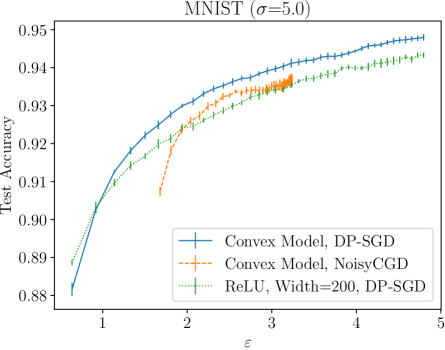
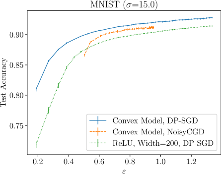
Figure 2: MNIST Comparisons: Test accuracies vs. the spent privacy budget $\varepsilon$, when $\delta=10^{-5}$ and each model is trained for 400 epochs. The ReLU network is a one hidden-layer fully connected network, and the batch size equals 1000 for all methods considered.

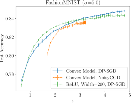
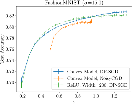
Figure 3: FashionMNIST Comparisons: Test accuracies vs. the spent privacy budget $\varepsilon$, when $\delta=10^{-5}$ and each model is trained for 400 epochs. The model is a one hidden-layer fully connected ReLU network and the batch size equals 1000 for all methods considered.

6 Conclusions and Outlook

We have shown how to privately approximate the two-layer ReLU network, and we have given first high privacy-utility trade-off results for the noisy cyclic mini-batch GD. As shown by the experiments on benchmark image classification datasets, the results for the convex problems have a similar privacy-utility trade-off as the models obtained by applying DP-SGD to a one hidden-layer ReLU network and using the composition analysis for DP-SGD. This is encouraging as the convexification opens up the possibility of considering also other private convex optimizers. Theoretically, an interesting future task is to carry out end-to-end utility analysis for private optimization of ReLU networks via the dual form. The recent non-private results by Kim and Pilanci, (2024) show connections between the stochastic approximation of the dual form and the ReLU minimization problem.

One possible limitation of the proposed method is the additional compute and memory cost. Finding ways to tune the number of random hyperplanes could possibly mitigate this. An interesting general question is, whether it is possible to obtain better privacy-utility trade-off for the final model by using the privacy amplification by iteration type of analysis than by using the composition analysis for DP-SGD. Our experimental observation is that the stagnation of learning and the plateauing of the $(\varepsilon,\delta)$-privacy guarantees for the final model happen approximately at the same time. In order to get a better understanding of this question, more accurate privacy amplification by iteration analysis for DP-SGD or for the noisy cyclic mini-batch GD could be helpful, as the $(\varepsilon,\delta)$-composition bounds for DP-SGD cannot likely be improved a lot.

Appendix A Reference Algorithm for the Utility Bounds

Algorithm 1 Differentially Private Gradient Descent (Song et al.,, 2021)

1:  Input: dataset $D=\{D_{i}\}_{i=1}^{n}$, loss function $\ell\,:\,\mathbb{R}^{p}\times\mathcal{X}\rightarrow\mathbb{R}$, gradient $\ell_{2}$-norm bound $L$, constraint set $\mathcal{C}\subseteq\mathbb{R}^{p}$, number of iterations $T$, noise variance $\sigma^{2}$, learning rate $\eta$.

2:  $\theta_{0}\leftarrow 0$.

3:  for $t=0,\ldots,T-1$ do

4:     $g^{\textrm{priv}}_{t}\leftarrow\frac{1}{n}\sum\limits_{i=1}^{n}\partial_{\theta}\ell(\theta_{t},d_{i})+b_{t}$, where $b_{t}\sim\mathcal{N}(0,\sigma^{2}I_{d})$.

5:     $\theta_{t+1}\leftarrow\Pi_{\mathcal{C}}\left(\theta_{t}-\eta\cdot g^{\textrm{priv}}_{t}\right)$, where $\Pi_{\mathcal{C}}(v)=\mathrm{argmin}_{\theta\in\mathcal{C}}\left\lVert\theta-v\right\rVert_{2}.$

6:  end for

7:  return $\theta^{\textrm{priv}}=\frac{1}{T}\sum\limits_{t=1}^{T}\theta_{t}.$

Appendix B Proof of Lemma 2

Lemma 1.

The gradients of the gradients of the loss function

$$\ell(v,x_{j},y_{j})=\frac{1}{2}\left\lVert\sum\nolimits_{i=1}^{P}(D_{i})_{jj}x_{j}^{T}v_{i}-y_{j}\right\rVert_{2}^{2}+\frac{\lambda}{2}\sum\nolimits_{i=1}^{P}\left\lVert v_{i}\right\rVert_{2}^{2}$$

are $\beta$-Lipschitz continuous for $\beta=\left\lVert x_{j}\right\rVert_{2}^{2}+\lambda$.

Proof.

For the quadratic function

$$h(v)=\frac{1}{2}\left\lVert\sum\nolimits_{i=1}^{P}(D_{i})_{jj}x_{j}^{T}v_{i}-y_{j}\right\rVert_{2}^{2}$$

the Hessian matrix is of the diagonal block form

$$\nabla^{2}h=\mathrm{diag}\left(A_{1},\ldots,A_{P}\right),$$

where $A_{i}=x_{j}D_{i}^{2}x_{j}^{T}=x_{j}D_{i}x_{j}^{T}$. Since for all $i\in[P]$, $x_{j}D_{i}x_{j}^{T}\preccurlyeq x_{j}x_{j}^{T}$, $\nabla^{2}h\preccurlyeq x_{j}x_{j}^{T}$ and furthermore for the spectral norm of $\nabla^{2}h$ we have that $\left\lVert\nabla^{2}h\right\rVert_{2}\leq\left\lVert x_{j}x_{j}^{T}\right\rVert_{2}=\left\lVert x_{j}\right\rVert_{2}^{2}$. ∎

Appendix C Utility Bound: Random Data

We give a convergence analysis for the minimization of the loss function

$$h(v)=\frac{1}{2}\left\lVert\sum\limits_{i=1}^{P}D_{i}Xv_{i}-y\right\rVert_{2}^{2}$$

without any constraints. Kim and Pilanci, (2024) have recently given several results for the stochastic approximations of the convex problem (3.3). The analysis uses the condition number $\kappa$ defined as

$$\kappa=\frac{\lambda_{\max}(XX^{T})}{\lambda_{\min}(M)},$$

where

$$M=\mathbb{E}_{g\sim\mathcal{N}(0,I_{d})}[\mathrm{diag}[\mathds{1}(Xg\geq 0)]XX^{T}\mathrm{diag}[\mathds{1}(Xg\geq 0)]].$$

Lemma 1 (Kim and Pilanci, 2024, Proposition 2).

Suppose we sample $P\geq 2\kappa\log\frac{n}{\delta}$ hyperplane arrangement patterns and assume $M$ is invertible. Then, with probability at least $1-\delta$, for any $y\in\mathbb{R}^{n}$, there exist $v_{1},\ldots,v_{P}\in\mathbb{R}^{d}$ such that

$$\sum\limits_{i=1}^{P}D_{i}Xv_{i}=y.$$ (C.1)

Furthermore, if we assume random data, i.e., $X_{ij}\sim\mathcal{N}(0,1)$ i.i.d., then for sufficiently large $d$ we have the following bound for $\kappa$.

Lemma 2 (Kim and Pilanci, 2024, Corollary 3).

Let the ratio $c=\frac{n}{d}\geq 1$ be fixed. For any $\gamma>0$, there exists $d_{1}$ such that for all $d\geq d_{1}$ with probability at least $1-\gamma-\frac{1}{(2n)^{8}}$,

$$\kappa\leq 10\sqrt{2}\left(\sqrt{c}+1\right)^{2}.$$

There results together tell that taking $d$ and $n$ large enough (such that $n\geq d$), we have that with $P={O}(\frac{n\log\frac{n}{\gamma}}{d})$ hyperplane arrangements we get the zero global optimum with high probability, i.e., there exists $u\in\mathbb{R}^{d\cdot P}$ such that Eq. (C.1) holds with probability at least $1-\gamma-\frac{1}{(2n)^{8}}$.

In case $d$ and $n$ are large enough and we choose $P={O}\left(\frac{n\log\frac{n}{\gamma}}{d}\right)$ hyperplane arrangements, we have that $p=d\cdot P={O}(n\log\frac{n}{\gamma})$ and we directly get the following corollary.

Theorem 3.

For any $\gamma>0$, there exists $d_{1}$ such that for all $d\geq d_{1}$, $n\geq d$, with probability at least $1-\gamma-\frac{1}{(2n)^{8}}$,

$$\mathcal{L}(\theta^{\textrm{priv}},X)-\mathcal{L}(\theta^{*},X)\leq\widetilde{O}\left(\frac{1}{\sqrt{n}\varepsilon}\right),$$

where $\widetilde{O}$ omits logarithmic factors.

Appendix D Proof of Lemma 3

Lemma 1.

For a data-matrix $X\in\mathbb{R}^{n\times d}$, label vector $y\in\mathbb{R}^{n}$ and a regularization parameter $\lambda>0$, consider the ReLU minimization problem

$$\min_{\{u_{j},\alpha_{j}\}_{j=1}^{m}}\frac{1}{2}\left\lVert\sum\nolimits_{j=1}^{m}\phi(Xu_{j})\alpha_{j}-y\right\rVert_{2}^{2}+\frac{\lambda}{2}\left(\sum\nolimits_{j=1}^{m}\left\lVert u_{j}\right\rVert_{2}^{4}+\alpha_{j}^{4}\right).$$ (D.1)

Then, the problem (D.1) and the problem

$$\min_{\{u_{j},\alpha_{j}\}_{j=1}^{m},\left\lVert u_{j}\right\rVert_{2}\leq 1\forall j\in[m]}\frac{1}{2}\left\lVert\sum\nolimits_{j=1}^{m}\phi(Xu_{j})\alpha_{j}-y\right\rVert_{2}^{2}+\lambda\left(\sum\nolimits_{j=1}^{m}\alpha_{j}^{2}\right)$$ (D.2)

have equal minima.

Proof.

From Young’s inequality $\left\lVert x\right\rVert_{2}^{2}+\left\lVert y\right\rVert_{2}^{2}\geq 2\langle a,b\rangle$ it follows that

$$\frac{\lambda}{2}\left(\sum\nolimits_{j=1}^{m}\left\lVert u_{j}\right\rVert_{2}^{4}+\alpha_{j}^{4}\right)\geq\lambda\sum\nolimits_{j=1}^{m}\left\lVert u_{j}\right\rVert_{2}^{2}\cdot\alpha_{j}^{2}.$$

We see that the problem (D.1) is scaling invariant, i.e., for any solution $\{u_{j}^{*},\alpha_{j}^{*}\}_{j=1}^{m}$ and for any $\gamma_{i}>0$, $i\in[m]$, also $\{u_{j}^{*}\cdot\gamma_{i},\alpha_{j}^{*}/\gamma_{i}\}_{j=1}^{m}$ gives a solution. Choosing for every $i\in[m]$, $\gamma_{i}=\sqrt{\frac{\alpha_{i}}{\left\lVert u_{j}\right\rVert_{2}}}$ gives an equality in Young’s inequality. Since this scaling does not affect the solution, we must have for the global minimizer $\{u_{j}^{*},\alpha_{j}^{*}\}_{j=1}^{m}$ of the ReLU minimization problem (D.1) that

$$\frac{1}{2}\left\lVert\sum\nolimits_{j=1}^{m}\phi(Xu_{j}^{*})\alpha_{j}^{*}-y\right\rVert_{2}^{2}+\frac{\lambda}{2}\left(\sum\nolimits_{j=1}^{m}\left\lVert u_{j}^{*}\right\rVert_{2}^{4}+(\alpha_{j}^{*})^{4}\right)$$ (D.3)

$$= \frac{1}{2}\left\lVert\sum\nolimits_{j=1}^{m}\phi(Xu_{j}^{*})\alpha_{j}^{*}-y\right\rVert_{2}^{2}+\lambda\left(\sum\nolimits_{j=1}^{m}\left\lVert u_{j}^{*}\right\rVert_{2}^{2}(\alpha_{j}^{*})^{2}\right).$$

Again, due to the scaling invariance, we see that the minimizing the right-hand-side of (D.3) w.r.t. $\{u_{j},\alpha_{j}\}_{j=1}^{m}$ is equivalent to the problem (D.2).

∎

Appendix E Non-DP MNIST Experiment: Stochastic Approximation of the Dual Problem

Figure 5 illustrates the approximability of the stochastic approximation for the dual problem in the non-private case, when the number of random hyperplanes $P$ is varied, for the MNIST classification problem described in Section 5. We apply SGD with batch size 1000 to both the stochastic dual problem and to a fully connected ReLU network with hidden-layer width 200, and for each model optimize the learning rate in the grid $\{10^{-i/2}\}$, $i\in\mathbb{Z}$. This non-private comparison shows that the approximabilty of the stochastic dual problem increases with increasing $P$, and suggests that the benefits in the private case become from the effect of convexification and not from a better approximability of the network.

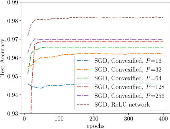
Figure 4: Test accuracies vs. number of epochs, when all models are trained using SGD with batch size 1000. The number of random hyperplanes $P$ is varied for the stochastic dual problem. The ReLU network is a one hidden-layer fully connected ReLU network with hidden-layer width 200. Cross-entropy loss is used for all models.

Appendix F DP MNIST Experiment: Stochastic Approximation of the Dual Problem

Figure 5 illustrates the approximability of the stochastic approximation for the dual problem in the private case, when the number of random hyperplanes $P$ is varied, for the MNIST classification problem described in Section 5. We apply DP-SGD with batch size 1000 to both the stochastic dual problem and to a fully connected ReLU network with hidden-layer width 200, and for each model optimize the learning rate in the grid $\{10^{-i/2}\}$, $i\in\mathbb{Z}$. Based on these comparisons, we choose $P=128$ for all the experiments of Section 5.

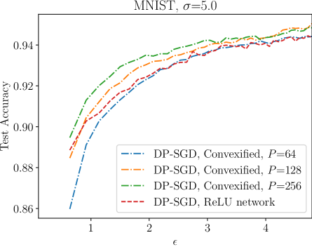
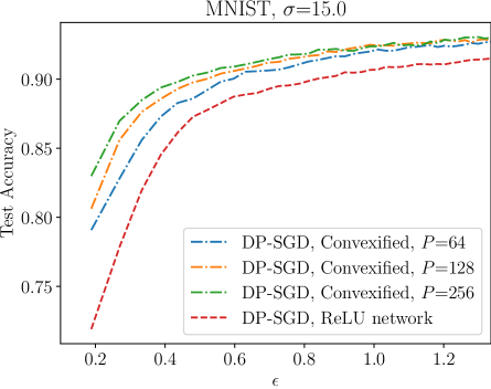
Figure 5: Test accuracies vs. number of epochs, when all models are trained using DP-SGD with batch size 1000, for two different noise levels $\sigma$. The number of random hyperplanes $P$ is varied for the stochastic dual problem. The ReLU network is a one hidden-layer fully connected ReLU network with hidden-layer width 200.

Appendix G Comparison of PLD and RDP Accounting for Subsampling Without Replacement

Instead of using the numerical approach described in Section 2 of the main text, we could alternatively compute the $(\varepsilon,\delta)$-DP guarantees for DP-SGD with subsampling without replacement using the RDP bounds given by Wang et al., (2019). Fig. 6 illustrates the differences when $\sigma=5.0$ and ratio of the batch size and total dataset size $m/n$ equals 0.01. The RDP parameters are converted to $(\varepsilon,\delta)$-bounds using the conversion formula of Lemma 1.

Lemma 1 (Canonne et al., 2020).

Suppose the mechanism $\mathcal{M}$ is $\big{(}\alpha,\epsilon^{\prime}\big{)}$-RDP. Then $\mathcal{M}$ is also $(\epsilon,\delta(\epsilon))$-DP for arbitrary $\epsilon\geq 0$ with

$$\delta(\epsilon)=\frac{\exp\big{(}(\alpha-1)(\epsilon^{\prime}-\epsilon)\big{)}}{\alpha}\left(1-\frac{1}{\alpha}\right)^{\alpha-1}.$$ (G.1)

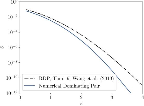
Figure 6: $(\varepsilon,\delta)$-DP guarantees for DP-SGD with subsampling without replacement, computed using the RDP bound of Wang et al., (Thm. 9, 2019) and the numerical dominating pair computed using the privacy profile bound of Zhu et al., (2022) and the numerical algorithm by Doroshenko et al., (2022). The parameter $\sigma=5.0$ and ratio of the batch size and total dataset size $m/n$ equals 0.01.

Bibliography

- (1) Abadi, M., Chu, A., Goodfellow, I., McMahan, H. B., Mironov, I., Talwar, K., and Zhang, L. (2016a). Deep learning with differential privacy. In Proceedings of the 2016 ACM SIGSAC Conference on Computer and Communications Security, pages 308–318.
- (2) Abadi, M., Chu, A., Goodfellow, I., McMahan, H. B., Mironov, I., Talwar, K., and Zhang, L. (2016b). Deep learning with differential privacy. In Proceedings of the 2016 ACM SIGSAC conference on computer and communications security, pages 308–318.
- Asoodeh et al., (2020) Asoodeh, S., Diaz, M., and Calmon, F. P. (2020). Privacy amplification of iterative algorithms via contraction coefficients. In 2020 IEEE International Symposium on Information Theory (ISIT), pages 896–901. IEEE.
- Avella-Medina et al., (2023) Avella-Medina, M., Bradshaw, C., and Loh, P.-L. (2023). Differentially private inference via noisy optimization. The Annals of Statistics, 51(5):2067–2092.
- Balle et al., (2019) Balle, B., Barthe, G., Gaboardi, M., and Geumlek, J. (2019). Privacy amplification by mixing and diffusion mechanisms. Advances in neural information processing systems, 32.
- Bartan and Pilanci, (2019) Bartan, B. and Pilanci, M. (2019). Convex relaxations of convolutional neural nets. In ICASSP 2019-2019 IEEE International Conference on Acoustics, Speech and Signal Processing (ICASSP), pages 4928–4932. IEEE.
- Bassily et al., (2019) Bassily, R., Feldman, V., Talwar, K., and Guha Thakurta, A. (2019). Private stochastic convex optimization with optimal rates. Advances in Neural Information Processing Systems, 32.
- Bassily et al., (2021) Bassily, R., Guzmán, C., and Menart, M. (2021). Differentially private stochastic optimization: New results in convex and non-convex settings. Advances in Neural Information Processing Systems, 34.
- Bassily et al., (2014) Bassily, R., Smith, A., and Thakurta, A. (2014). Private empirical risk minimization: Efficient algorithms and tight error bounds. In Proceedings of the 2014 IEEE 55th Annual Symposium on Foundations of Computer Science, FOCS ’14, pages 464–473, Washington, DC, USA. IEEE Computer Society.
- Bok et al., (2024) Bok, J., Su, W., and Altschuler, J. M. (2024). Shifted interpolation for differential privacy. arXiv preprint arXiv:2403.00278.
- Cai et al., (2021) Cai, T. T., Wang, Y., and Zhang, L. (2021). The cost of privacy: Optimal rates of convergence for parameter estimation with differential privacy. The Annals of Statistics, 49(5):2825–2850.
- Canonne et al., (2020) Canonne, C., Kamath, G., and Steinke, T. (2020). The discrete gaussian for differential privacy. In Advances in Neural Information Processing Systems.
- Chen et al., (2020) Chen, X., Wu, S. Z., and Hong, M. (2020). Understanding gradient clipping in private SGD: A geometric perspective. Advances in Neural Information Processing Systems, 33:13773–13782.
- Chourasia et al., (2021) Chourasia, R., Ye, J., and Shokri, R. (2021). Differential privacy dynamics of langevin diffusion and noisy gradient descent. Advances in Neural Information Processing Systems, 34.
- Chua et al., (2024) Chua, L., Ghazi, B., Kamath, P., Kumar, R., Manurangsi, P., Sinha, A., and Zhang, C. (2024). How private is DP-SGD? arXiv preprint arXiv:2403.17673.
- Dong et al., (2022) Dong, J., Roth, A., and Su, W. J. (2022). Gaussian differential privacy. Journal of the Royal Statistical Society Series B, 84(1):3–37.
- Doroshenko et al., (2022) Doroshenko, V., Ghazi, B., Kamath, P., Kumar, R., and Manurangsi, P. (2022). Connect the dots: Tighter discrete approximations of privacy loss distributions. Proceedings on Privacy Enhancing Technologies, 4:552–570.
- Dwork et al., (2006) Dwork, C., McSherry, F., Nissim, K., and Smith, A. (2006). Calibrating noise to sensitivity in private data analysis. In Proc. TCC 2006, pages 265–284.
- Ergen et al., (2023) Ergen, T., Gulluk, H. I., Lacotte, J., and Pilanci, M. (2023). Globally optimal training of neural networks with threshold activation functions. In The Eleventh International Conference on Learning Representations.
- Ergen and Pilanci, (2021) Ergen, T. and Pilanci, M. (2021). Global optimality beyond two layers: Training deep relu networks via convex programs. In International Conference on Machine Learning, pages 2993–3003. PMLR.
- Feldman et al., (2018) Feldman, V., Mironov, I., Talwar, K., and Thakurta, A. (2018). Privacy amplification by iteration. In 2018 IEEE 59th Annual Symposium on Foundations of Computer Science (FOCS), pages 521–532. IEEE.
- Gopi et al., (2021) Gopi, S., Lee, Y. T., and Wutschitz, L. (2021). Numerical composition of differential privacy. In Advances in Neural Information Processing Systems.
- Kim and Pilanci, (2024) Kim, S. and Pilanci, M. (2024). Convex relaxations of relu neural networks approximate global optima in polynomial time. arXiv preprint arXiv:2402.03625.
- Koskela et al., (2023) Koskela, A., Heikkilä, M., and Honkela, A. (2023). Numerical accounting in the shuffle model of differential privacy. Transactions on machine learning research.
- Koskela et al., (2021) Koskela, A., Jälkö, J., Prediger, L., and Honkela, A. (2021). Tight differential privacy for discrete-valued mechanisms and for the subsampled gaussian mechanism using FFT. In International Conference on Artificial Intelligence and Statistics, pages 3358–3366. PMLR.
- LeCun et al., (1998) LeCun, Y., Bottou, L., Bengio, Y., and Haffner, P. (1998). Gradient-based learning applied to document recognition. Proceedings of the IEEE, 86(11):2278–2324.
- Liu et al., (2023) Liu, X., Jain, P., Kong, W., Oh, S., and Suggala, A. (2023). Label robust and differentially private linear regression: Computational and statistical efficiency. Advances in Neural Information Processing Systems, 36.
- Mishkin et al., (2022) Mishkin, A., Sahiner, A., and Pilanci, M. (2022). Fast convex optimization for two-layer relu networks: Equivalent model classes and cone decompositions. In International Conference on Machine Learning, pages 15770–15816. PMLR.
- Nasr et al., (2021) Nasr, M., Songi, S., Thakurta, A., Papemoti, N., and Carlin, N. (2021). Adversary instantiation: Lower bounds for differentially private machine learning. In 2021 IEEE Symposium on Security and Privacy (SP), pages 866–882. IEEE.
- Pilanci and Ergen, (2020) Pilanci, M. and Ergen, T. (2020). Neural networks are convex regularizers: Exact polynomial-time convex optimization formulations for two-layer networks. In International Conference on Machine Learning, pages 7695–7705. PMLR.
- Redberg et al., (2024) Redberg, R., Koskela, A., and Wang, Y.-X. (2024). Improving the privacy and practicality of objective perturbation for differentially private linear learners. Advances in Neural Information Processing Systems, 36.
- Song et al., (2021) Song, S., Steinke, T., Thakkar, O., and Thakurta, A. (2021). Evading the curse of dimensionality in unconstrained private glms. In International Conference on Artificial Intelligence and Statistics, pages 2638–2646. PMLR.
- Sordello et al., (2021) Sordello, M., Bu, Z., and Dong, J. (2021). Privacy amplification via iteration for shuffled and online PNSGD. In Joint European Conference on Machine Learning and Knowledge Discovery in Databases, pages 796–813. Springer.
- Talwar et al., (2014) Talwar, K., Thakurta, A., and Zhang, L. (2014). Private empirical risk minimization beyond the worst case: The effect of the constraint set geometry. arXiv preprint arXiv:1411.5417.
- Varshney et al., (2022) Varshney, P., Thakurta, A., and Jain, P. (2022). (nearly) optimal private linear regression for sub-gaussian data via adaptive clipping. In Conference on Learning Theory, pages 1126–1166. PMLR.
- Wang et al., (2022) Wang, Y., Lacotte, J., and Pilanci, M. (2022). The hidden convex optimization landscape of regularized two-layer relu networks: an exact characterization of optimal solutions. In International Conference on Learning Representations.
- Wang et al., (2019) Wang, Y.-X., Balle, B., and Kasiviswanathan, S. P. (2019). Subsampled Rényi differential privacy and analytical moments accountant. In The 22nd International Conference on Artificial Intelligence and Statistics, pages 1226–1235.
- Xiao et al., (2017) Xiao, H., Rasul, K., and Vollgraf, R. (2017). Fashion-mnist: a novel image dataset for benchmarking machine learning algorithms. arXiv preprint arXiv:1708.07747.
- Ye and Shokri, (2022) Ye, J. and Shokri, R. (2022). Differentially private learning needs hidden state (or much faster convergence). Advances in Neural Information Processing Systems, 35:703–715.
- Zhu et al., (2022) Zhu, Y., Dong, J., and Wang, Y.-X. (2022). Optimal accounting of differential privacy via characteristic function. Proceedings of The 25th International Conference on Artificial Intelligence and Statistics.