Signatures of supermassive charged gravitinos
in liquid scintillator detectors

Abstract

In previous work two of the present authors have suggested possible experimental ways to search for stable supermassive particles with electric charges of ${\mathcal{O}}(1)$ in upcoming underground experiments and the new JUNO observatory in particular [K.A. Meissner and H. Nicolai, Eur. Phys. J. C 84, 269 (2024)]. In this paper we present a detailed analysis of the specific signature of such gravitino-induced events for the JUNO detector. The proposed method of detection relies on the ‘glow’ produced by photons during the passage of such particles through the detector liquid, which would last for about a few to a few hundred microseconds depending on its velocity and the track. The cross sections for electronic excitation of the main component of the scintillator liquid, namely linear alkylbenzene (LAB), by the passing gravitino, are evaluated using quantum-chemical methods. The results show that, if such particles exist, the resulting signals would lead to a unique and unmistakable signature, for which we present event simulations as they would be seen by the JUNO photomultipliers. Our analysis brings together two very different research areas, namely fundamental particles physics and the search for a fundamental theory on the one hand, and methods of advanced quantum chemistry on the other.

I Introduction

Following the suggestion Meissner and Nicolai (2019a) that Dark Matter (or DM, for short) could consist at least in part of an extremely dilute gas of supermassive stable gravitinos with charge $\pm\frac{2}{3}e$, possible experimental signatures of the passage of such particles through underground detectors were examined in Meissner and Nicolai (2024) (see also Meissner and Nicolai (2023) where an outlier event reported by the MACRO collaboration Ambrosio12 et al. (2004) was investigated as possible evidence towards the existence of such a new particle). The suggestion of superheavy gravitinos as DM is chiefly motivated by the remarkable match between the fermion content of the Standard Model (SM) of particle physics with three generations of 16 quarks and leptons on the one hand, and the spin-$\frac{1}{2}$ states of the $N\!=\!8$ supermultiplet associated to maximally extended supergravity on the other hand R. Jackiw and Witten (1985) (see also Nicolai and Warner (1985)). This agreement and the link with $N\!=\!8$ supergravity lead to the prediction that the only extra fermions beyond the observed 48 spin-$\frac{1}{2}$ fermions of the SM would be eight supermassive gravitinos, which carry fractional electric charges Meissner and Nicolai (2015, 2018).

In this paper we analyze options for a dedicated search for slowly moving supermassive charged gravitinos in much more detail than has been done before. We shall argue that the JUNO experiment An et al. (2016) is predestined for such a search, due to its special design and the properties of its scintillator liquid that would lead to signatures that could not have been seen so far with more conventional DM detectors using Argon or Xenon. JUNO is the largest underground detector ever constructed, with the main purpose of exploring the physics of (anti-)neutrinos (see An et al. (2016); Abusleme et al. (2022) for a detailed description of the experiment), and expected to start taking data in early 2025, this close date providing an extra incentive for the present work. From our perspective, JUNO stands out among other upcoming and planned such experiments because it offers unique opportunities to also search for exotic events of the type proposed here. Specifically, we will focus on a particular proposal for embedding the SM into a Planck scale unified theory, and investigate its possible experimental consequences. We will show that if supermassive particles with the properties predicted by this scheme do exist, the associated signatures would be very different from those induced by neutrino events, and could thus be easily discriminated with appropriate (and hopefully rather minor) adjustments of the JUNO electronics and triggering systems. It goes without saying that the actual discovery of these still hypothetical particles would constitute a major advance also in the search for a unified theory.

Our paper thus tries to predict, as accurately as possible and taking into account all relevant aspects, ways and means to search for weakly ionizing charged supermassive gravitinos with the JUNO detector. Remarkably, our analysis requires an interdisciplinary endeavor on the interface of particle physics and quantum chemistry, two areas which are usually considered to be far apart. The particle physics part of the paper involves a novel approach to physics beyond the SM which we review in section II, and relies on a still to be developed theoretical framework beyond quantum field theory, as well as mostly unexplored mathematics (hyperbolic Kac-Moody Lie algebras). The quantum chemistry part makes use of advanced methods and large computational resources to calculate the lowest excitation levels of the scintillator oil. The latter are needed for the precise determination of the emission rates of photons along the track of the gravitino in the detector, which in turn are crucial for the observability (or not) of such events. As it turns out, the specifics of the JUNO scintillator liquid play a key role in this computation. As a first step, the present analysis considers only the photons emitted from the lowest excitation levels of the scintillator oil. It thus gives only a lower bound on what could actually be seen, but this seems already sufficient to detect the gravitinos when they pass through the JUNO detector, provided the triggering and software are appropriately designed. In future work we will discuss further effects that may enhance the predicted signal (higher level excitations, ionization, etc.). We also explain the possible reasons why WIMP searches using solid state or liquid Argon detectors were unlikely to detect any such signals – not to mention the fact that the signals these experiments have been concentrating on are of an entirely different character! In the section on simulations we will also list possible caveats and difficulties that may still stand in the way of discovery, such as the dark count rates of the JUNO photomultiplier tubes (PMTs), or the ¹⁴C contamination of the detector liquid (whose concentration in the detector is bounded above by $2\cdot 10^{-17}$ according to most recent measurements Obe ).

Simulating the interactions between the scintillating medium and a passing supermassive gravitino is a complicated task, in part due to the existence of several competing processes. Apart from direct interactions with nuclei (nuclear recoil), the three main mechanisms by which the energy can be transferred from a charged particle (projectile) to a molecule in a liquid are: (i) excitation to a bound excited state of the molecule, (ii) capture of an electron by the projectile and its subsequent re-absorption by a molecular ion, and (iii) ionization, i.e. ejection of electron to the continuum Meissner and Nicolai (2024). In this work we will only discuss the first process. While the remaining two processes certainly contribute, we show that the first one alone may already lead to a signal which is strong enough to be detectable by JUNO. Therefore the results of our work should be considered as a very conservative lower bound on the signal strength, not a definitive quantitative prediction. In subsequent papers we shall consider the other mechanisms outlined above which may enhance the signal.

The organization of this paper is as follows. In Section II we list the main reasons for the gravitino DM hypothesis, and its main differences with more established ideas about DM, namely the huge mass and the ${\mathcal{O}}(1)$ electric charge of the proposed DM candidate. In the following sections we first briefly review the JUNO detector design and then study the interaction of the gravitino with the liquid scintillator medium. This enables us to explain the mechanism by which a passing gravitino leads to emission of light which may be subsequently detected. Next, by taking into account other factors that play a role in the detection, we theoretically predict the signature of the signal that the gravitino would produce. We discuss how the signal from the gravitino would differ from other events that may occur within the detector, in particular the inverse beta decays which JUNO was designed to record (Section IV). We argue that the signal produced by a gravitino passing through the detector is fairly unique and can be distinguished both from the background noise and, being much longer, from the inverse beta decay events or antineutrino interactions with the nuclei. Next, we use quantum-chemical methods to compute the relevant cross sections for electronic excitation caused by the gravitino, for both liquid argon detectors and JUNO. The case of argon is computationally much simpler and also potentially useful for possible future searches with such detectors. The details of the computational model and the quantum-chemical calculations are explained in Section V. Finally, in Section VI we present simulations describing how the JUNO PMTs could record a gravitino event. Here we provide results for the case of a gravitino with two assumed velocities corresponding the Earth velocity and the galactic velocity, respectively, to argue that even in this worse case of the Earth velocity the track produced by the gravitino can be unambiguously identified and clearly discriminated against background or neutrino induced events. Our simulations take into account background event rates due to the ¹⁴C contamination of the scintillator fluid as well as dark count rates of photomultipliers, both of which turn out to be much smaller (in the Earth velocity case) or negligible (in the galactic velocity case) than the signal. The final remarks and directions for future work are given in Section VII.

II Why supermassive charged gravitinos?

Because the proposed scenario differs substantially from more established ideas about DM, and for the reader’s convenience, we first review the main arguments for supermassive charged gravitinos and the gravitino DM hypothesis. This proposal has its origins in maximal $N\!=\!8$ supergravity Cremmer and Julia (1979); De Wit and Nicolai (1982) and relies in an essential way on the associated fermion multiplet comprising 56 helicity-$\frac{1}{2}$ and eight helicity-$\frac{3}{2}$ states (this supermultiplet is also distinguished by the cancellation of conformal anomalies Meissner and Nicolai (2017); Tseytlin (2013)). In comparison with currently popular proposals for extending the SM, which usually come with numerous new particles not too far above the electroweak scale (especially in the context of superstring unification and low energy supersymmetry), this scheme is very minimalistic in that the only extra fermions appearing beyond the 48 spin-$\frac{1}{2}$ fermions of the SM are eight supermassive gravitinos (which absorb eight spin-$\frac{1}{2}$ Goldstinos). Such a novel approach to unification and the DM problem appears amply justified in view of decades of failed attempts to discover any signs of new physics with more standard approaches to physics beyond the SM, most significantly the non-observation of new fundamental spin-$\frac{1}{2}$ degrees of freedom at LHC. A further hint in support of a minimalistic scheme is the fact that the RG evolution of the measured SM couplings up to the Planck scale exhibits no Landau poles (an apparent instability in the effective scalar potential generated by the RG evolution of the Higgs boson self-coupling can be cured by slightly modifying the scalar sector of the SM). This strongly indicates that, as far as its spin-$\frac{1}{2}$ and spin-1 sectors are concerned, the SM could simply survive more or less as is all the way up to the Planck scale – an option that is outside the scope of conventional GUT or superstring phenomenology.

In essence, the proposal goes back to Gell-Mann’s old observation that the fermion content of the SM with three, and only three, generations of quarks and leptons (including right-chiral neutrinos) can be matched with the spin-$\frac{1}{2}$ content of the maximal $N\!=\!8$ supermultiplet after removal of eight Goldstinos R. Jackiw and Witten (1985); Nicolai and Warner (1985). This surprising agreement constitutes the main theoretical motivation for the present proposal. Yet, it has not received much attention because of an overwhelming expectation that LHC and related experiments, as well as various DM searches, would discover, or at least produce indirect evidence for new fundamental degrees of freedom at the TeV scale, especially in connection with low energy ($N\!=\!1$) supersymmetry. The fact that all these searches have come up empty-handed despite enormous efforts strengthens the case for unification attempts such as the present one that try to make do with just the 48 SM spin-$\frac{1}{2}$ fermions.

Crucially, in Gell-Mann’s scheme the matching of U(1)_em charges requires a ‘spurion shift’ of $\delta q=\pm\frac{1}{6}$ R. Jackiw and Witten (1985); Nicolai and Warner (1985) that is not part of $N\!=\!8$ supergravity and that, in terms of the original spin-$\frac{1}{2}$ tri-spinor $\chi^{ijk}$ of $N\!=\!8$ supergravity, requires a very peculiar deformation of the supergravity U(1) with a generator that does not belong to the SU(8) $R$-symmetry of the theory Meissner and Nicolai (2015, 2018). Furthermore, it invokes a fictitious family symmetry SU(3)_f such that the supergravity fermions can only ‘see’ the diagonal subgroup of SU(3)_c and SU(3)_f. The main new step taken in Meissner and Nicolai (2018, 2019a) consisted in extending Gell-Mann’s considerations to the eight massive gravitinos which would be the only extra fermions beyond the known three generations of quarks and leptons. Under SU(3)$\,\times\,$U(1)_em the gravitinos transform as

$$\left({\bf 3}\,,\,\frac{1}{3}\right)\oplus\left(\bar{\bf 3}\,,\,-\frac{1}{3}\right)\oplus\left({\bf 1}\,,\,\frac{2}{3}\right)\oplus\left({\bf 1}\,,\,-\frac{2}{3}\right)$$ (1)

Importantly, the U(1)_em gravitino charge assignments in (1) include the spurion shift needed for matching the spin-$\frac{1}{2}$ sectors Meissner and Nicolai (2019a); see Meissner and Nicolai (2015, 2018) for a derivation of these quantum numbers and an explanation of how to extend the spurion shift to the gravitinos. All gravitinos would thus carry fractional electric charges. If one identifies the SU(3) in (1) with SU(3)_c as in Meissner and Nicolai (2019a), a complex triplet of gravitinos would be subject to strong interactions. The color triplet gravitinos (whose possible physical manifestations have been discussed in Meissner and Nicolai (2019b)) will not play any role in our subsequent considerations, so we will be concerned here only with the color singlet gravitinos of charge $\pm\frac{2}{3}e$.

Although the combined spin-$\frac{1}{2}$ and spin-$\frac{3}{2}$ content thus coincides with the fermionic part of the $N\!=\!8$ supergravity multiplet, it is important to stress that the underlying theory would need to be an as yet unknown extension beyond $N\!=\!8$ supergravity, because the latter theory cannot accommodate the required shift of U(1) charges, nor reproduce the SU(3)${}_{c}\times$ SU(2)${}_{w}\times$ U(1)_Y symmetry of the SM. The point of view taken here is that the required extension necessitates a framework beyond space-time based quantum field theory, and that rectification of the mismatches should be viewed as providing guidance towards such a theory. What seems clear is that such a theory will require extending known symmetries to infinite-dimensional symmetries, which may not admit a space-time realization. In particular, it is expected that the maximal rank hyperbolic Kac-Moody algebra E₁₀ and its ‘maximal compact’ sub-algebra K(E₁₀) will play a key role , and possibly supersede supersymmetry as a guiding principle towards unification. One strong hint in this direction is the fact that the requisite shift of U(1) charges necessarily requires enlarging the $R$-symmetry SU(8)$\,\equiv\,$ K(E₇) of $N\!=\!8$ supergravity all the way to K(E₁₀) Kleinschmidt and Nicolai (2015), which is hugely infinite-dimensional. At this time it is not clear how to go about constructing such a theory, but see Damour et al. (2002) for a closely related attempt in the context of maximal supergravity. From that construction it follows that conventional concepts of quantum field theory, as well as the SM symmetries and space-time itself, would then have to emerge from some pre-geometric ‘space-time-less’ scheme 

In view of the unresolved theoretical challenges we here adopt a more pragmatic approach by focusing on possible observable signatures induced by the spin-$\frac{3}{2}$ gravitinos which could support the above scenario. More specifically, an important consequence of (1) and the U(1) charge shift is that, due to their fractional charges the gravitinos cannot decay into SM fermions, and are therefore stable independently of their mass. Their stability against decays makes them natural candidates for DM Meissner and Nicolai (2019a). While most currently popular DM scenarios are based on the assumption of ultralight constituents (such as axions) or TeV scale WIMPs, the above arguments would suggest that DM could thus consist at least in part of an extremely dilute gas of supermassive stable gravitinos with charge $q=\pm\frac{2}{3}$ in units of the elementary charge $e$. In this case they must have very large mass, as follows directly from the bounds on the electric charge of any putative DM particle of large mass derived in McDermott et al. (2011); Dolgov et al. (2013); Del Nobile et al. (2016). Although these bounds were derived with a different perspective, namely bounding the charge of ‘low mass’ (in comparison with the Planck scale) DM candidates, by considering various astrophysical constraints, we are of course free to take the opposite view of this analysis as providing a lower bound on the mass of supermassive particles with given ${\mathcal{O}}(1)$ charges. This evidently constitutes an extrapolation well beyond the mass range considered in McDermott et al. (2011); Dolgov et al. (2013); Del Nobile et al. (2016), but the inequalities derived there nevertheless indicate that gravitinos with charges (1) can be within the allowed range to be viable DM candidates if their mass is close to, but still below, the Planck scale. The latter requirement is motivated by the fact that the very notion of a particle and its mass may become meaningless in a regime where classical space and time de-emerge.

As was argued in Meissner and Nicolai (2019a) the abundance of the color singlet gravitinos cannot be estimated since they were never in thermal equilibrium, but if they are the dominant contribution to the DM content of the universe one can plausibly assume their abundance in first approximation to be given by the average DM density inside galaxies Weber and de Boer (2010), viz.

$$\rho_{DM}\,\sim\,0.3\cdot 10^{6}\,\rm GeV\!\cdot\!m^{-3}$$ (2)

(the average in the Universe is a million times smaller). If DM were entirely made out of nearly Planck mass particles with an assumed mass of $10^{18}$ GeV, this would amount to $\sim 3\cdot 10^{-13}$ particles per cubic meter within galaxies. Furthermore assuming an average velocity of 30 km$\,\cdot\,$s^-1 this yields the flux estimate

$$\Phi\;\sim\;0.03\,{\rm m}^{-2}{\rm yr}^{-1}{\rm sr}^{-1}$$ (3)

We emphasize that, in addition to the unknown mass of the particle, there remain important uncertainties which could shift this estimate in either direction. One concerns possible inhomogeneities in the DM distribution within galaxies or stellar systems, which could lead to either a local depletion or to a local enhancement of the DM density (2) in the vicinity of the earth (see e.g. Damour and Krauss (1999) for an early discussion of this point). The other is the average velocity $v$ of superheavy DM particles w.r.t. the earth which we assume to lie in the range

$$v_{E}\,\lesssim\,v\,\lesssim\,v_{S}\,,$$ (4)

where $v_{E}$ is the virial velocity for a particle bound to the Sun and $v_{S}$ if it is bound to our Galaxy. In the paper we will assume $v_{E}=30$ km/s and $v_{S}=230$ km/s. It is also clear that a sufficiently heavy charged particle can easily pass through the earth without deflection, independently of the effects it has on ordinary matter. In particular, it can enter a detector from any direction. Because the velocities (4) are non-relativistic and the energy transfer from the particle to the molecule is on average below its ionization energy, ionization is a relatively rare event, which is our main reason for concentrating on electronic excitations to bound states within the molecule.

The distinctive feature of the present proposal is therefore hat the DM gravitinos do participate in SM interactions with couplings of order ${\mathcal{O}}(1)$. In this sense, these DM candidates are not dark at all, but simply too rare and too faint to be observed directly with standard devices because of their extremely low abundance. This is in contrast to other scenarios involving DM particles which are assumed to have only weak and gravitational interactions with SM matter, but might still be seen with standard detectors due to their more frequent occurrence. By contrast the gravitinos in (1) could in principle be detected if a way can be found to overcome their low abundance. A further obstacle is the low ionization rate of these particles, as explained above. It is here that a special feature of JUNO comes into play that may facilitate detection, namely the fact that the scintillator liquid has low excitation levels (because benzene is a large molecule), enabling even a weakly ionizing particle to produce a visible effect.

III Juno detector design

For the benefit of the readers who are not familiar with the design of liquid scintillator detectors, in this section we provide a brief overview of salient features of the JUNO detector design and operation principles. First, JUNO is tuned to detect signals from the inverse beta decay events in which an antineutrino $\bar{\nu}_{e}$ hits a proton in the detector medium and produces a neutron and a positron

$$\bar{\nu}_{e}+p\longrightarrow n+e^{+}.$$ (5)

The positron annihilates almost immediately when it encounters an electron and produces two $\gamma$ photons – the primary signal. The secondary signal is produced sometime later by the capture of the free neutron by an atomic nucleus.

The JUNO is built deep underground to shield it from the cosmic radiation and consists of two major parts. The first is the central detector which is spherical in shape and has a diameter of $35.5\,$m. It is filled with the scintillating liquid comprising three ingredients: linear alkylbenzenes (LAB, solvent), 2,5-diphenyloxazole (PPO, $3\,$g/L) and 1,4-Bis(2-methylstyryl)benzol (Bis-MSB, 15 mg/L). As the $\gamma$ photons produced in the events travel through the detector, they undergo Compton scattering and transfer some energy to the molecules of the scintillating liquid which thereby gets electronically excited. As the LAB molecules are the most abundant in the liquid, they absorb most of the energy of the passing photon. The radiative lifetime of LAB molecules is large (hundreds of nanoseconds) and hence they have enough time to transfer their energy to the main fluor (PPO) through direct collisions. The fluor molecule rapidly emits a photon (wavelength $\approx 350\,$nm) as a result of de-excitation from the first excited to the ground electronic state. Finally, the Bis-MSB molecules serve as wavelength shifters. They absorb the photons emitted by PPO and, with a small delay, re-emit photons with somewhat different wavelength. The purpose of this process is to shift the photon wavelength to values where the photon detectors (PMTs) are the most sensitive. The central detector is covered with photomultiplier tubes which capture the photons emitted inside.

The second part of the JUNO detector is a cylindrical tank of diameter $\approx 38\,$m in which the central (spherical) detector is embedded. The tank is filled with ultrapure water and is used to detect the Cherenkov radiation emitted when high-energy particles, primarily muons, pass through. When the Cherenkov radiation is detected in the water tank, all photomutiplier tubes in the main detector which are on the path of the incoming particle are switched off. This procedure, called vetoing, is the main mechanism which enables to reduce the background noise resulting from, e.g. radioactivity of the surrounding rock and soil.

IV Detection of the gravitino

It is clear that the gravitino particle possesses different physical characteristics than the antineutrinos which the JUNO detector was designed to detect. As a result, the signal generated by the gravitino will be different from the inverse beta decay events. In this section we shall discuss these differences from the qualitative point of view, while in subsequent sections we present results of the calculations which enable to quantify the strength of the gravitino signal.

The first major difference in the gravitino detection is related to the vetoing mechanism. As discussed in Refs. Meissner and Nicolai (2020, 2024) gravitino moves at much lower velocities than the background muons, much less than 1% of the speed of light in vaccum. It is well known that the Cherenkov radiation is emitted only when a particle travels in a medium with a velocity larger than the speed of light in this medium. The speed of light in a medium is smaller by a factor of $1/n$ than in vacuum, where $n$ is the refractive index of the medium. For water (which fills the outer tank of the detector) the refractive index is roughly $n\approx 1.33$ which means that the speed of light in water is about 75% of the speed in vacuum. This velocity is much larger than that of the gravitino which means that the passing gravitino will not emit the Cherenkov radiation.

Nonetheless, the gravitino passing through the outer tank will excite the neighboring water molecules to higher electronic states. By subsequent radiative decay, water molecules may emit photons which are detected by the photomutiplier tubes. However, as the de-excitation of liquid water is dominated by non-radiative decay channels and the outer tank contains no fluor molecules, the efficiency of this process is extremely low. Moreover, the orientation of the photons potentially emitted by water molecules is completely random. This is different from the Cherenkov radiation which is emitted in a cone with the opening angle $\cos\theta=1/n\beta$, where $\beta$ is the ratio between the speed of the particle and the speed of light in vacuum. For these two reasons, we argue that the passing gravitino will not trigger the vetoing mechanism in the outer tank.

Next, the passing gravitino enters the inner part of the detector filled with the scintillating mixture. It excites the surrounding LAB molecules which transfer the excitation to the PPO fluor through collisions. Light emitted by the radiative decay of the fluor is detected in the PMTs (after absorption and re-emission by the wavelength shifter). On the surface, this mechanism is very similar to the inverse beta decay events where the LAB molecules are excited by Compton scattering, while the subsequent steps are identical. However, we argue that the inverse beta decay events can be distinguished from gravitino events based on their entirely different temporal characteristics.

The $\gamma$ photons generated by the inverse beta decay events travel trough the detector at roughly 66% of speed of light in vacuum, because the refractive index of the scintillating liquid is about $n\approx 1.5$. As the inverse beta decay events can occur at an arbitrary point in the inner detector, the two $\gamma$ photons have to travel, on average, the distance equal to the radius of the detector, $R\approx 17.7\,$m. Therefore, it takes about $90\,$ns before the $\gamma$ photons leave the detector. All LAB molecules are excited within this time and it takes another couple of nanoseconds for the excitation transfer and decay of the PPO molecule. Therefore, the whole primary signal is over within roughly $100\,$ns. If the secondary signal resulting from the capture of the free neutron by atomic nucleus (and subsequent decay of the deuteron) is observed, another $\gamma$ photon is generated after about $250\,$ns from the primary event. The secondary signal is over after another $\approx 100\,$ns. In total, one would observe two strong signals lasting $\approx 100\,$ns separated by about $250\,$ns, and the whole event would last less than a microsecond.

The situation is quite different in the case of gravitinos. As mentioned above, they move at a much lower velocity, estimated at considerably less then 1% of the speed of light. In fact, more rigorous velocity estimates were established in the previous section by assuming that DM particles are bound either to the Solar System or to the Milky Way galaxy, leading to $v_{E}=29.8\,$km/s and $v_{S}=230\,$km/s, respectively. When expressed as a fraction of the speed of light, these velocities correspond to $\beta_{E}\approx 10^{-4}$ and $\beta_{S}\approx 7.7\cdot 10^{-4}$. This means that the gravitino needs either about $600\,\mu$s (for $v_{E}$) or about $77\,\mu$s (for $v_{S}$) to complete the run through the inner detector, assuming that the average distance it has to travel is equal to roughly the radius of the inner sphere. This corresponds to time scales larger by two or three orders of magnitude in comparison with the inverse beta decay events.

This difference in time scales can be used to distinguish the inverse beta decay events (and other events involving fast particles) from the gravitino events. Due to its enormous mass, the gravitino would move at nearly constant speed along a linear path. Every now and then, the LAB molecule is excited and this excitation is transferred to the PPO fluor which emits a photon. After, on average, roughly $100\,$ns from the LAB excitation, this photon reaches the photomultiplier tubes and can be detected. By this time the gravitino travels a certain distance and has a chance of exciting another LAB molecule, hence the process repeats itself. The signal will last for tens of microseconds up to a fraction of a milisecond, rather than less than a microsecond as in the inverse beta decay signals or the antineutrino interaction with nuclei.

In the above analysis, we have assumed that the signal generated by the gravitino is strong enough to be observable by the JUNO detector. This depends entirely on the number of photons generated per unit distance as the gravitino travels through the scintillating fluid. To estimate this quantity, knowledge of the number of LAB molecules excited by the gravitino to a higher electronic state is required. In the next section, we develop a theoretical framework which enables to calculate this crucial parameter.

V Theory of molecular excitations

V.1 Preliminary considerations

As the interaction of the gravitino with the scintillating medium is a complicated process, approximations have to be introduced to make theoretical predictions feasible. In this section we introduce and justify the approximations introduced into the theoretical model.

First, it is instructive to consider the time and energy scales involved in the interaction of the gravitino with a charge-neutral molecule. First, regarding the energy scale, in the preceding paper Meissner and Nicolai (2024) it has been discussed that in a simple classical picture, the maximum energy transferred from the gravitino to an electron in a molecule is of the order of several eV for $\beta\approx 10^{-3}$ or less. This corresponds to the energy range of electronic excitations to bound excited states, whereas ionization events are expected to be relatively unimportant. In other words, the passing gravitino can be treated as a perturbation, similarly as with the interaction of weak external electric field.

Of course, this perturbative picture is not valid in situations where the gravitino penetrates deep within the $1s$ core orbitals of carbon, oxygen, etc. atoms. In such cases, the excitation of the core electron leaves a vacancy filled by an electron from a higher energy level (Auger effect) and an ionization event is possible. However, such events are expected to be rare due to relatively compact extent of the core orbitals in comparison with the valence shells. For example, the volume of a single water molecule calculated as the volume of a union of spheres corresponding with the van der Waals radii of two hydrogen and an oxygen atoms equals to about $26$ų Maglic and Lavendomme (2022) (geometry of water in liquid taken from Ref. Moriarty and Karlström (1997)). The effective radius of the water molecule is hence equal to about $1.8$Å. By comparison, the $1s$ core orbital of the oxygen atom is characterized by the mean electron-nucleus distance of $\langle r\rangle=0.105$Å Saito (2009). Due to the exponential decay of the orbital with the electron-nucleus distance, a sphere of radius $2\langle r\rangle=0.210$Å centered at the atomic nucleus encloses nearly total core density ($\approx\,$94%). The probability of the collision with the core relative to the collision with the whole molecule is equal to the square of the ratio of the corresponding effective radii and evaluates to only about $1$%. For larger molecules, such as LAB, this ratio turns out to be even lower. Therefore, even if the core penetration events are not described accurately by our model, this should have a negligible effect on the overall results, justifying the perturbative approach.

The second issue which warrants a discussion is the strength of the interaction between the molecules in a liquid in relation with the energy transfer from the gravitino. In the inner detector, interaction between LAB molecules is dominated by the $\pi$-$\sigma$ and $\pi$-$\pi$ dispersion interactions (London forces), because the permanent dipole moment of LAB is very small. The strength of this type of interactions is usually of the order of $10-15\,$kJ/mol, for example, $11.3\,$kJ/mol for the benzene dimer Pitonak et al. (2008) and $14.5\,$kJ/mol for the toluene dimer Rogers et al. (2006). Therefore, the intermolecular interaction energies in the scintillating medium, on average, are smaller than $0.01\,$eV – two to three orders of magnitude less than the expected energy transfer from the passing gravitino. This leads to the conclusion that it is reasonable to neglect the intermolecular interactions in modeling the excitations caused by the gravitino.

Table 1: Components of LAB with general formula C₆H₅CHR₁R₂ and their molar concentrations.

Overall formula	Concentration	R1	R2
C6H5-C10H21	10%	CH3	C8H17
		C2H5	C7H15
		C3H7	C6H13
		C4H9	C5H11
C6H5-C11H23	35%	CH3	C9H19
		C2H5	C8H17
		C3H7	C7H15
		C4H9	C6H13
		C5H11	C5H11
C6H5-C12H25	35%	CH3	C10H21
		C2H5	C9H19
		C3H7	C8H17
		C4H9	C7H15
		C5H11	C6H13
C6H5-C13H27	20%	CH3	C11H23
		C2H5	C10H21
		C3H7	C9H19
		C4H9	C8H17
		C5H11	C7H15
		C6H13	C6H13

Table 2: Excitation energies and oscillator strengths for the $S_{1}$ state of the LAB isomers. The order of the isomers is the same as in Table 1 (from top to bottom). The results for the proposed LAB model molecule (3-PP) are given in the last row, while averaged results for $20$ isomers are given in the second last row. All results were obtained at the ADC(2)/aug-cc-pVTZ level of theory using B3LYP-D3/cc-pVTZ optimized geometries.

Isomer	Excitation energy (eV)	Osc. strength $\cdot\,10^{4}$
1	5.195	6.49
2	5.184	7.33
3	5.183	7.25
4	5.182	8.20
5	5.194	6.35
6	5.185	7.25
7	5.183	7.35
8	5.182	7.55
9	5.183	8.12
10	5.194	6.31
11	5.185	7.37
12	5.183	7.11
13	5.182	7.45
14	5.182	7.58
15	5.195	6.29
16	5.185	7.26
17	5.183	7.17
18	5.182	7.26
19	5.182	7.48
20	5.183	8.17
average	5.185	7.27
3-PP	5.186	7.68

Next, we consider the time scale related to the gravitino-molecule interaction. One can easily estimate that when the gravitino is, say, $10\,$Å from the molecular center, the strength of the resulting interaction is too small to cause any electronic excitation. Then assuming even the lowest velocity estimate of $\beta_{E}\approx 10^{-4}$, it takes only a few tens of femtoseconds for the gravitino to travel from the initial distance of $10\,$Å from the molecule to the distance of $10\,$Å on the other side. Within this regime, energy transfer from the gravitino to the LAB molecule is possible, leading to electronic excitations. However, during such a short time the nuclei of a molecule can be considered as essentially static. This leads to the important conclusion that we can consider only adiabatic electronic excitations caused by the gravitino and treat atomic nuclei to be essentially motionless during the process. The subsequent nuclear relaxation and other transformations occur at much longer time scales and by that time, the gravitino is already far away from a molecule.

Finally, we have to introduce a model suitable for description of the gravitino. The proposed gravitino is a point-like particle of charge $\pm\frac{2}{3}e$ and enormous mass $Mc^{2}\approx 10^{18}\,$GeV. Therefore, the loss of the kinetic energy of the gravitino due to energy transfer to the scintillating medium (estimated at several eV per molecule, see above) is negligible. Therefore, one can assume that the gravitino moves along a predefined linear path with a constant velocity on the scale of the whole detector. Additionally, due to the huge mass, one can treat the gravitino simply as a source of a moving classical Coulomb potential, neglecting the quantum effects such as tunneling etc. In fact, a more rigorous treatment would be based on the Liénard–Wiechert potential which takes into account the retardation effects. However, the correction to the Coulomb potential resulting from the retardation is of the leading order $\beta^{2}$ which is negligible for the gravitino with the estimated $\beta\ll 10^{-2}$.

V.2 Model linear alkylbenzene molecule

The main component of the scintillating medium in the inner detector (LAB) is not a single molecule, but rather a mixture of various isomers with the general chemical formula C₆H₅-C_nH_2n+1 with $n=10-13$. In this work, we use that the composition of LAB given in Ref. Lombardi et al. (2019) for the pilot distillation and stripping tests at Daya Bay Neutrino Laboratory for their future use in the JUNO detector. In Table 1 we provide a listing of the $20$ possible isomers of LAB identified by us based on Ref. Lombardi et al. (2019) along with their stated overall concentrations.

Due to the large number of isomers and their considerable size, we seek a simpler model molecule that captures the essential characteristics of LAB. In particular, we focus on the first excited singlet state ($S_{1}$) of LAB. While the passing gravitino causes excitations also to higher excited electronic states, they are expected to be relatively unstable compared to $S_{1}$ and quickly decay non-radiatively due to non-adiabatic and collisional processes. Taking into consideration that the time required to transfer the energy from LAB to the PPO fluor is of the order of nanoseconds, we expect the $S_{1}$ state to be the primary carrier of the excess energy. Of course, the decay of higher excited electronic states of LAB undoubtedly leads to an increase population of the $S_{1}$ state, but neglect of such events can be seen as a conservative lower bound to the overall efficiency of the process. In a follow-up work, we shall consider excitations to higher electronic states, as well as other competing processes such as electron capture.

To study the variation of the properties of the $S_{1}$ state among the LAB isomers, we first optimized the ground-state geometry of each isomer using the B3LYP density functional Becke ; Lee et al. (1988); Vosko et al. (1980) with the D3 dispersion correction Grimme et al. (2010, 2011); Smith et al. (2016) and the cc-pVTZ basis set Dunning Jr (1989). These calculations were performed with the help of the QChem program package Shao et al. (2015). The optimized structures of each isomer are given in Supplemental Material sup . Next, the vertical excitation energy to the $S_{1}$ state, denoted $\omega_{1}$, and the corresponding oscillator strength of the dipole transition

$$f_{01}=\frac{4\omega_{1}}{3}|\boldsymbol{\mu}_{01}|^{2},$$ (6)

where $\boldsymbol{\mu}_{01}$ is the dipole $S_{0}\rightarrow S_{1}$ transition moment, was calculated for each isomer using the algebraic-diagrammatic construction method Schirmer (1982); Trofimov et al. (2006); Hättig and Hald (2002); Dreuw and Wormit (2015), ADC(2), within the aug-cc-pVTZ basis set Kendall et al. (1992). In Table 2 we list the results obtained for every isomer. Clearly, the variation of the results among the isomers is tiny in the case of the excitation energies and amounts to no more than $0.02\,$eV. A larger spread is obtained in the case of the oscillator strengths, but even for this quantity the maximum deviation from the mean is of the order of $10\%$. From the chemical point of view, this similarity among LAB isomers is straightforward to understand. The excitation to the $S_{1}$ state is dominated by the $\pi\rightarrow\pi^{*}$ transition within the benzene ring. The alkyl substitution groups serve as weak electron donors, but do not alter the excitation character. We can exploit this property by restricting our consideration to a simpler model molecule that captures the essential properties of the $S_{1}$ state. For this purpose, we propose the 3-phenylpentane (3-PP) molecule with the chemical formula C₆H₅CH(C₂H₅)₂. In Table 2 we provide the excitation energy and the oscillator strength for the $S_{0}\rightarrow S_{1}$ transition in the 3-PP molecule calculated at the same level of theory as for the actual LAB constituents. As one can see, the properties of the 3-PP are very close to the average of the corresponding properties of LAB isomers.

V.3 Excitation probability due to the passing gravitino

The main unknown quantity determining the possibility of detecting the proposed gravitino particle in the JUNO detector is the probability that the LAB molecules in the inner detector are electronically excited by the passing DM particle. To specify the model used to calculated this probability from first principles, we rely on the assumptions and estimates outlined in Sec. V.1. First, we neglect the interactions between the molecules in the scintillating liquid and hence consider interaction of an isolated model LAB molecule (3-PP) with the gravitino. The gravitino is treated classically as a moving charge interacting with all electrons and nuclei in the molecule through the Coulomb potential

$$V_{\mathrm{DM}}(t)=-\sum_{i}\frac{q}{|\mathbf{r}_{i}-\mathbf{s}(t)|}+\sum_{A}\frac{qZ_{A}}{|\mathbf{R}_{A}-\mathbf{s}(t)|},$$ (7)

where the summation indices $i$ and $A$ run over all electrons and nuclei, respectively, in the molecule, $Z_{A}$ are the nuclear charges, and $\mathbf{s}(t)$ is the fixed path of the gravitino. An explicit parametrization of the latter quantity will be specified later, but for now it suffices to write $\mathbf{s}(t)=\mathbf{s}_{0}+\mathbf{v}t$, where $\mathbf{v}$ is the velocity of the gravitino and $\mathbf{s}_{0}$ is the point at which the gravitino is the closest to the origin of the coordinate system. The origin can be chosen arbitrarily – this choice has no influence on the final results after proper averaging over the path of the gravitino is performed. For simplicity, in the present work the nuclear position was chosen in the case of argon atom, while the nuclear center of charge was used for LAB model. In this parametrization, both in the $t\rightarrow\infty$ and $t\rightarrow-\infty$ limits the gravitino is infinitely far away from the atom/molecule. Conversely, for $t=0$ the grativino distance to the chosen origin $\mathbf{s}_{0}$ is minimal along the path.

Time evolution of the system is governed by the Schrödinger equation

$$i\partial_{t}\Psi(\mathbf{r},\mathbf{R},t)=\hat{H}\Psi(\mathbf{r},\mathbf{R},t),$$ (8)

where $\mathbf{r}$ and $\mathbf{R}$ is a shorthand notation for coordinates of all electrons and nuclei, respectively, in the system. The total Hamiltonian of the system is a sum of the electronic Hamiltonian for the isolated molecule $(H_{0})$ and the interaction potential with the gravitino

$$\hat{H}=\hat{H}_{0}+V_{\mathrm{DM}}(t).$$ (9)

As discussed in Sec. V.1 the effective time of the interaction between the gravitino and the molecule is small and nuclear motion can be neglected. Therefore, the total wavefunction is expanded into a linear combination of adiabatically excited electronic states

$$\Psi(\mathbf{r},\mathbf{R}_{0},t)=\sum_{n=0}^{\infty}c_{n}(t)\,e^{-iE_{n}t}\,\psi_{n}(\mathbf{r},\mathbf{R}_{0}),$$ (10)

where $\mathbf{R}_{0}$ is the reference geometry of the molecule. The phase factor $e^{-iE_{n}t}$ in the above formula is arbitrary and was included for convenience. The states $\psi_{n}(\mathbf{r},\mathbf{R}_{0})$ are eigenfunctions of the molecular Hamiltonian

$$\hat{H}_{0}\psi_{n}(\mathbf{r},\mathbf{R}_{0})=E_{n}\psi_{n}(\mathbf{r},\mathbf{R}_{0}),$$ (11)

where $E_{n}\equiv E_{n}(\mathbf{R}_{0})$ is the electronic energy of the state $n$. According to the arguments from Sec. V.1 we assume that the $V_{\mathrm{DM}}(t)$ can be treated as a perturbation and solve Eq. (8) using the time-dependent perturbation theory. We expand the coefficients $c_{n}(t)$ in the orders of the perturbation

$$c_{n}(t)=c_{n}^{(0)}(t)+c_{n}^{(1)}(t)+\ldots$$ (12)

and treat $\hat{H}_{0}$ and $V_{\mathrm{DM}}(t)$ as a zeroth-order and a first-order quantity, respectively. Additionally, the unperturbed system is assumed to reside in the ground electronic state, i.e. $c_{n}^{(0)}(t)=\delta_{n0}$. As in the first Born approximation, time derivative of the amplitudes are found from

$$\dot{c}_{n}^{(1)}(t)=e^{-i\omega_{n}t}\langle\psi_{n}|V_{\mathrm{DM}}(t)|\psi_{0}\rangle.$$ (13)

We are interested in values of the coefficients $c_{n}(t)$ for $t\rightarrow\infty$, i.e. when the gravitino gets far away from the molecule. To this end, we integrate both sides of the above expression over time within the interval $t\in(-\infty,+\infty)$ and use the fact that $\lim_{t\rightarrow-\infty}c_{n}^{(1)}(t)=\delta_{0n}$. This leads to (for $n\geq 1$)

$$c_{n}^{(1)}\equiv\lim_{t\rightarrow\infty}c_{n}^{(1)}(t)=\int_{-\infty}^{\infty}dt\;e^{-i\omega_{n}t}\,\langle\psi_{n}|V_{\mathrm{DM}}(t)|\psi_{0}\rangle.$$ (14)

We are interested in the probability $p_{0\rightarrow n}$ that the molecule is found in the excited state $n$ when the gravitino gets far away, i.e. the perturbation is effectively switched off (adiabatically). It is given by the expression

$$p_{0\rightarrow n}=|c_{n}^{(1)}|^{2}.$$ (15)

The present method of calculation of the transition probabilities is based directly on Eq. (14). Evaluation of the key quantity, $\langle\psi_{n}|V_{\mathrm{DM}}(t)|\psi_{0}\rangle$, requires two main ingredients. The first is the transition density matrix from the ground state to the $n$-th excited state. In this work, it was evaluated using the ADC(2) method employing a truncation scheme identical to Ref. Mester et al. (2018). The second ingredient are the matrix elements of the Coulomb potential $V_{\mathrm{DM}}(t)$ within the current atomic basis. As the Gaussian basis set are used exclusively in this work, the required integrals can be evaluated analytically Boys (1950); McMurchie and Davidson (1978) and LibInt2 library Valeev (2024) was employed for this purpose.

This leaves only the integration over time which is performed numerically on a uniform grid with spacing $\Delta t=0.1$. We verified that further decrease of $\Delta t$ leads to no appreciable changes in the overall results. The integral over time is approximated by truncating it according to $\int_{-\infty}^{\infty}dt\approx\int_{-T}^{T}dt$, and the value of $T$ is chosen adaptively (for each path separately) such that the calculated transition probabilities are stable to within threshold of $10^{-13}$. While this approach is straightforward is the case of argon and water, for LAB molecules a large $T$ was required to achieve convergence. In order to accelerate the calculations, whenever the gravitino is separated by more than $400\,$ bohr from the molecular center, the quantity $\langle\psi_{n}|V_{\mathrm{DM}}(t)|\psi_{0}\rangle$ is evaluated using the multipole expansion of the potential $V_{\mathrm{DM}}(t)$ rather than by direct calculations. In the present work, the multipole expansion was truncated at quadrupole terms. This leads to an error vanishing as inverse fourth power of the gravitino-molecule separation which is negligible for the present purposes. Further technical details of the procedure of evaluating $p_{0\rightarrow n}$, along with analysis of additional approximations which can be applied to reduce the cost of the calculations, are beyond the scope of the present paper and will be reported separately.

V.4 Gravitino path averaging

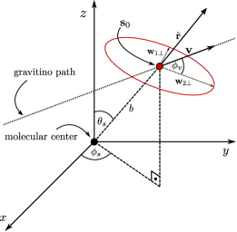
Figure 1: Parametrization of the path of the gravitino adopted in the present work.

To faithfully model the interaction of the gravitino with the scintillating medium, we have to take into account the fact that the gravitino encounters roughly $10^{9}$–$10^{12}$ molecules along its track which are randomly oriented with respect to the path. Therefore, the excitation probabilities $p_{0\rightarrow n}$ defined in the previous section have to be averaged over all possible path orientations.

As discussed in the previous section, the path of the gravitino is parametrized as $\mathbf{s}(t)=\mathbf{s}_{0}+\mathbf{v}t$, where $\mathbf{s}_{0}$ is the point at which the gravitino is the closest to the adopted origin of the coordinate system. Therefore, there are five degrees of freedom in specifying the path – one additional degree has already been eliminated by fixing the origin of the coordinate system (removing the translation of the system as a whole). Two variables that parameterize the path come up naturally in the present context. The first is the velocity of the gravitino, $v=|\mathbf{v}|$, and the second is the so-called impact parameter, $b=|\mathbf{s}_{0}|$, which is simply the minimal distance between the gravitino and the molecular center of charge along the path. Note that the definition of $\mathbf{s}_{0}$ implies that the dot product $\mathbf{v}\cdot\mathbf{s}_{0}$ is equal to zero.

This leaves three degrees of freedom to be specified. As the next two variables we choose angles $\theta_{s}\in[0,\pi]$ and $\phi_{s}\in[0,2\pi]$ which are the coordinates of the vector $\mathbf{s}_{0}$ in the spherical coordinate system centered at the origin, i.e. $\mathbf{s}_{0}=b\,[\sin\theta_{s}\cos\phi_{s},\sin\theta_{s}\sin\phi_{s},\cos\theta_{s}]=b\,\hat{\mathbf{s}}_{0}$, where $\hat{\mathbf{s}}_{0}$ is unit vector. For better clarity, we decided to express $\hat{\mathbf{s}}_{0}$ in Cartesian coordinates, $\hat{\mathbf{s}}_{0}=[x_{0},y_{0},z_{0}]$, in the subsequent formulas.

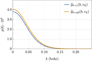
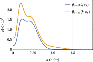
Figure 2: Excitation probabilities $\widetilde{p}_{0\rightarrow 1}(b,v)$ and $\widetilde{p}_{0\rightarrow\mathrm{all}}(b,v)$ for the argon atom as a function of the impact parameter, $b$. The results for the gravitino velocities $v_{E}$ and $v_{S}$ are given in the left and right panel, respectively. All values are in atomic units. Notice a different scale on the vertical axis of both plots.

The fifth, and final, variable is the angle $\phi_{v}\in[0,2\pi]$ which rotates the path of the gravitino within a plane that passes through $\mathbf{s}_{0}$ and is perpendicular to the vector pointing from the origin to the point $\mathbf{s}_{0}$. One can show by direct calculation that the following vectors lie within this plane and are orthonormal:

$$\mathbf{w_{1\perp}}=\frac{[1,\;0,\;-x_{0}/z_{0}]}{\sqrt{1+x_{0}^{2}/z_{0}^{2}}}$$

$$\mathbf{w_{2\perp}}=\frac{[x_{0}y_{0}/z_{0},\;-x_{0}^{2}/z_{0}-z_{0},\;y_{0}]}{\sqrt{\frac{x_{0}^{2}}{z_{0}^{2}}(x_{0}^{2}+y_{0}^{2})+2x_{0}^{2}+y_{0}^{2}+z_{0}^{2}}}$$

While this choice of $\mathbf{w}_{1\perp}$ and $\mathbf{w}_{2\perp}$ is not unique, it is convenient in practice. Note that the definitions given above break down when $z_{0}=0$. However, in this special case one can set $\mathbf{w}_{1\perp}=[0,0,1]$ and $\mathbf{w}_{2\perp}=[-y_{0},x_{0},0]$ without loss of generality. Finally, the last parameter specifying the path is the angle $\phi_{v}$ is defined such that:

$$\hat{\mathbf{v}}=\frac{\mathbf{v}}{|\mathbf{v}|}=\mathbf{w}_{1\perp}\cos\phi_{v}+\mathbf{w}_{2\perp}\sin\phi_{v}.$$ (16)

The definition of the variables specifying the path is illustrated graphically in Fig. 1.

To ease the presentation of the results we define the excitation probability $\widetilde{p}_{0\rightarrow n}(b,v)$ averaged over the angles $\theta_{s}$, $\phi_{s}$, and $\phi_{v}$ according to the formula

$$\widetilde{p}_{0\rightarrow n}(b,v)=\int_{0}^{\pi}d\theta_{s}\;\sin\theta_{s}\int_{0}^{2\pi}d\phi_{s}\int_{0}^{2\pi}d\phi_{v}\;p_{0\rightarrow n},$$ (17)

where the integrand is defined through Eq. (15). In the current implementation, this averaging is carried out numerically – we use the Lebedev quadrature Lebedev (1976, 1977); Lebedev and Laikov (1999) with 302 points for integration over the solid angle $(\theta_{s},\phi_{s})$ and the trapezoidal rule with 30 points and equal grid spacing for integration over $\phi_{v}$.

In the last step, the excitation probabilities have to be averaged over the impact parameter, $b$. For simplicity, we assume that the scintillating medium in the inner detector consists solely of LAB with the bulk density $0.8650\,$g/cm³ at $T=300\,$K Lombardi et al. (2019). The fluor and wavelength shifter molecules can be neglected in this analysis due to their low concentrations. Using the average molecular mass of LAB equal to $M_{\mathrm{LAB}}=241.52\,$g/mol, see Table 1, this leads to the density $\rho_{\mathrm{LAB}}=2.157\cdot 10^{27}\,$m^-3 expressed as the number of molecules per unit volume. Similarly, we use $\rho_{\mathrm{Ar}}=2.136\cdot 10^{28}\,$m^-3 for liquid argon. The distribution of molecules in the detector medium is assumed to be perfectly uniform. In the remainder of this section, we consider LAB molecules as an example, but analogous definitions hold also for liquid argon.

As the gravitino travels the distance $d$ through the inner detector, it encounters

$$dn_{\mathrm{LAB}^{*}}=2\pi d\,\rho_{\mathrm{LAB}}\,b\,db,$$ (18)

LAB molecules with respect to which the gravitino path is characterized by the impact parameter in the interval $[b,b+db]$. Therefore, to find the total number of LAB molecules which get excited, $n_{\mathrm{LAB}^{*}}$, we have to evaluate the integral

$$\begin{split}n_{\mathrm{LAB}^{*}}&=\int_{0}^{\infty}dn_{\mathrm{LAB}^{*}}\;\widetilde{p}_{0\rightarrow 1}(b,v)\\ &=2\pi d\,\rho_{\mathrm{LAB}}\int_{0}^{\infty}db\;b\,\widetilde{p}_{0\rightarrow 1}(b,v),\end{split}$$ (19)

where we restrict ourselves only to the first excited state of LAB. Further in the paper, we consider cross sections defined as

$$\sigma_{\mathrm{LAB}^{*}}(v)=2\pi\int_{0}^{\infty}db\;b\,\widetilde{p}_{0\rightarrow 1}(b,v),$$ (20)

such that $n_{\mathrm{LAB}^{*}}=d\,\rho_{\mathrm{LAB}}\,\sigma_{\mathrm{LAB}^{*}}(v)$. Note that the cross section $\sigma_{\mathrm{LAB}^{*}}(v)$ has units of m² and can be interpreted as the probability of exciting LAB to the first excited state per unit distance the gravitino travels and per single LAB molecule.

In the next two sections we report the calculated excitation probabilities and total cross sections for argon and model LAB molecule, while the corresponding results for water molecule are given in the Supplemental Material sup . On a technical note, the excitation energies and excited state wavefunctions required in $\widetilde{p}_{0\rightarrow 1}(b,v)$ were evaluated using the ADC(2) method Schirmer (1982); Trofimov et al. (2006); Hättig and Hald (2002); Dreuw and Wormit (2015) using the aug-cc-pVXZ basis set family Dunning Jr (1989); Kendall et al. (1992). We used X=Q for argon atom while X=T was employed for the remaining systems. To reduce the cost of the calculations, density-fitting approximation of the two-electron integrals Whitten (1973); Dunlap et al. (1979); Vahtras et al. (1993); Feyereisen et al. (1993); Rendell and Lee (1994); Kendall and Früchtl (1997); Weigend (2002) was invoked. The matching aug-cc-pVXZ-RIFIT basis sets optimized in Ref. Weigend et al. (1998, 2002) were used for this purpose. The error resulting from the density-fitting approximation is negligible in the present context.

V.5 Excitation cross-sections: argon

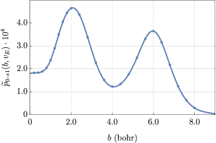
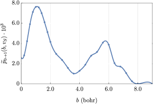
Figure 3: Excitation probabilities $\widetilde{p}_{0\rightarrow 1}(b,v)$ for model LAB molecule as a function of the impact parameter, $b$. The results for the gravitino velocities $v_{E}$ and $v_{S}$ are given in the left and right panel, respectively. All values are in atomic units. Notice a different scale on the vertical axis of both plots.

As a warm-up exercise we first consider liquid argon because the relevant computations are considerably simpler, as no elaborate path averaging procedure is required. For this case, excitation probabilities were evaluated for two gravitino velocities ($v_{E}$ and $v_{S}$). In the case of $v_{E}$, 32 values of $b$ were considered within the interval $b\in[0.0,0.50]$. For $v_{S}$ this grid is somewhat larger ($45$ points within interval $b\in[0.0,2.5]$) due to more rapid variation of the excitation probabilities as a function of $b$. As the path averaging is not necessary for argon, we calculated transition probabilities not only to the first excited state, i.e. $\widetilde{p}_{0\rightarrow 1}(b,v)$, but also to all bound states supported by a given basis (with excitation energies lower than the ionization energy of the atom calculated by the same method). The total excitation probability is then obtained by summing the excitation probabilities $\widetilde{p}_{0\rightarrow n}(b,v)$ for all accessible $n$. We denote this quantity by the symbol $\widetilde{p}_{0\rightarrow\mathrm{all}}(b,v)$. The excitation probabilities $\widetilde{p}_{0\rightarrow 1}(b,v)$ and $\widetilde{p}_{0\rightarrow\mathrm{all}}(b,v)$ are given in Fig. 2 for the velocities $v_{E}$ and $v_{S}$, respectively. Clearly, the transition to the first excited state dominates, especially for the lower velocity of the gravitino. This suggests that the effects such as ionization are likely negligible.

In the calculation of the cross sections, we employ the total excitation probabilities $\widetilde{p}_{0\rightarrow\mathrm{all}}(b,v)$. In order to perform integration over the impact parameter $b$ according to Eq. (20) we interpolate the results obtained on a grid using cubic $B$-spline method Press et al. (1992). The integration in Eq. (20) is then elementary and gives (in units of m²)

$$\begin{split}&\sigma_{\mathrm{Ar}^{*}}(v_{E})=6.84\cdot 10^{-27},\\ &\sigma_{\mathrm{Ar}^{*}}(v_{S})=1.73\cdot 10^{-24},\end{split}$$ (21)

for the velocities $v_{E}$ and $v_{S}$, respectively. From the point of view of simulations described in the next section, it is useful to define a related quantity, namely the mean time between the excitation events as the gravitino travels through the scintillating medium. This characteristic time can be calculated from the formula

$$\tau_{\mathrm{Ar}^{*}}(v)=\frac{1}{v\,\sigma_{\mathrm{Ar}^{*}}(v)\rho_{\mathrm{Ar}}},$$ (22)

and in the present case it equals

$$\begin{split}&\tau_{\mathrm{Ar}^{*}}(v_{E})=228\,{\rm ns}\\ &\tau_{\mathrm{Ar}^{*}}(v_{S})=0.12\,{\rm ns}.\end{split}$$ (23)

The argon-based experiments performed up to now had a relatively small size. Bigger detectors, such as the one with 20 t of LAr at Gran Sasso Manthos (2023), searching for WIMPs in the intermediate mass range, are still in the early phase of development. As we can see from (23), at least for galactic velocities, the number of photons produced by excitations in LAr can be significant. In principle there is therefore considerable potential for discovery of gravitinos also in the LAr experiments, which has been mainly limited by the size of the detector.

As one can see from inspection of the relevant numbers for liquid argon, there is in principle also a potential for discovery with more conventional detectors. If the particles in question actually exist, the absence of any signal so far in these experiments is therefore most likely due to (1) the much smaller surface area of existing DM detectors (which diminishes event rates by more than a factor of 100 in comparison with JUNO), (2) the much shorter duration of the passage of the particle through the detector, and (3) the fact that the relative closeness of its path to the walls of the detector (in comparison with JUNO) may not allow to clearly identify a trajectory, which could thus have been easily misidentified as background. Last but not least, the fact that these experiments did not expressly look for effects with a longer duration induced by atomic excitations, rather focusing on nuclear-recoil-induced events may have prevented a discovery even if a supermassive gravitino had actually passed through the detector. Similar comments apply to xenon-based detectors, as well as detectors using purified water.

V.6 Excitation cross-sections: LAB scintillator

Analogous calculations were performed for the LAB model molecule for velocities $v_{E}$ and $v_{S}$, and this is the main result we want to report in this work. We used the a grid of $b$ with spacing $0.2$ within the interval $(0.0,2.0)$ (where the excitation probabilities are the largest), and with spacing $0.4$ within the interval $(2.0,9.0)$. Beyond the point $b=9.0$, the excitation probabilities decay rapidly and are negligible for both velocities. The results for the model LAB molecule are illustrated in Fig. 3.

For integration over $b$, we used the same approach as in the case of argon atom. This leads to the averaged cross sections (in m²)

$$\begin{split}&\sigma_{\mathrm{LAB}^{*}}(v_{E})=5.62\cdot 10^{-23},\\ &\sigma_{\mathrm{LAB}^{*}}(v_{S})=5.74\cdot 10^{-22},\end{split}$$ (24)

and characteristic times

$$\begin{split}&\tau_{\mathrm{LAB}^{*}}(v_{E})=0.27\,{\rm ns}\\ &\tau_{\mathrm{LAB}^{*}}(v_{S})=0.0035\,{\rm ns}.\end{split}$$ (25)

These results are employed in the simulations described in the next section. Note that the excitation probabilities reported in this work never exceed a few parts per thousand, even at the peak $b$ and in the case of the larger velocity $v_{S}$. This suggests that the excitation process is indeed perturbative in nature and the adopted theoretical framework is justified. Note that by comparing the results for argon and LAB, i.e. Eqs. (23) and (25), it is immediately evident that the photon production rates for LAB are (much) higher than the ones for argon, which is another significant advantage of JUNO in comparison with previous experiments.

VI Simulations

In this section we provide some examples of simulations that show how the photons produced by a gravitino traversing the detector would be registered by the JUNO PMTs. As was shown in the previous section, the excitations of the scintillator oil with its admixtures of PPO and Bis-MSB on average produce a large number of photons per nanosecond along the track of the gravitino which strongly depends on the velocity of the gravitino. Specifically, we simulate the events for two velocities; galactic one assumed to be 230 km/s ($\beta\sim 7.7\cdot 10^{-4}$) and 29.8 km/s ($\beta\sim 10^{-4}$). For these exemplary values we have produced simulations with the following assumptions, based on the information provided in Ref. An et al. (2016):

• The photons produced by a passing gravitino along the track are emitted in random directions every 0.0035 ns (for $\beta_{S}$) or 0.27 ns (for $\beta_{E}$) as shown in Eq. (25);

• the overall efficiency of the photomultipliers is 30.1%;

• the area coverage by large (20”) PMTs is 75%;

• the attenuation coefficient of photons in the oil is given by $\exp(-l/l_{a})$ with $l_{a}$=27 m;

• the radioactive ¹⁴C has a concentration ¹⁴C/¹²C of at most $2\cdot 10^{-17}$ Obe ;

• dark count rates are counted separately for two types of 20” PMTs used in the central detector, namely Hamamatsu (5000 PMTs) and NNTV (12612 PMTs) Abusleme et al. (2022).

Other sources of photons, like ²³⁸U chain, ²³²Th chain, ²¹⁰Pb chain, ⁸⁵Kr contaminations as well as external sources, like radiation from surrounding rocks, are not included in the simulations. The flashes from antineutrinos and muons are very intense but very short-lived, and should be subtracted if they occur during the passage of a gravitino.

Based on these assumptions we get the average number of photons coming from the passage of gravitino and detected by large PMTs:

$$0.301\cdot 0.75\cdot 0.9/(0.0035\ {\rm ns}) \sim 58/{\rm ns}\;\;\;\;\,\mbox{for}\;\;\beta_{E},\;\;\;\;\;\;$$ (26)

$$0.301\cdot 0.75\cdot 0.9/(0.27\ {\rm ns}) \sim 0.75/{\rm ns}\;\;\mbox{for}\;\;\beta_{S},\;\;\;\;\;\;$$ (27)

where the first factor in the numerator corresponds to the PMT efficiencies, the second to the area coverage and the third to the approximate contribution from the attenuation in the oil. The time of passage for a gravitino crossing the detector along the diagonal would be 160 $\mu$s for $\beta=7.7\cdot 10^{-4}$ and 1260 $\mu$s for $\beta=10^{-4}$ so the number of photons detected should be $\sim$ 3.5 million in the first case and almost a million in the second. For tracks close to the edge, like the one we have chosen for simulations as described below, these numbers will be proportionally smaller but the relative importance of both ¹⁴C decays and the dark count rates is the same in all cases.

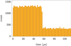
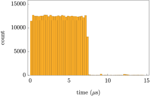
Figure 4: Number of detected photons as a function of time for velocities $v_{E}$ (left panel) and $v_{S}$ (right panel).

VI.1 Effects of ¹⁴C contamination

We have taken into account the decays ${}^{14}\mathrm{C}\rightarrow\,^{14}\mathrm{N}+e^{-}+\bar{\nu}$, assuming a relative ¹⁴C/¹²C concentration of $2\cdot~{}10^{-17}$ (representing an upper bound Obe ), and ¹⁴C half-life of $1.2\cdot 10^{11}$ s. This gives, on average, 0.143 decays per microsecond inside the detector, assuming the mass of oil equal to $2\cdot 10^{7}$ kg. The actual number of photons depends on the fraction $x$ of the energy carried away by the electron (with a maximal value of 156 keV), for which we use the beta distribution

$$P(x;p,q)\,=\,\frac{x^{p-1}(1-x)^{q-1}}{{\rm B}(p,q)}\qquad(0\leq x\leq 1),$$ (28)

where the energy of the electron is $x\cdot$156 keV. Inspection of the distribution curve given in Kuzminov and Osetrova (2000) shows that the best fit for the ¹⁴C decays is achieved with the parameter values $p=1.2$ and $q=2.7$ and the number of photons emitted is assumed to be ten photons per every keV of electron’s energy. Assuming that the ¹⁴C decay gives on average 49 keV (i.e. 490 photons) we have the following approximate number of photons per microsecond detected by large PMTs

$$0.143\cdot 490\cdot 0.301\cdot 0.75/\mu{\rm s}\sim 0.016/{\rm ns}.$$ (29)

As we see in Eq. (26) this value is roughly 3000 times smaller than the photon detection rate from $v_{S}$ gravitinos and 40 times smaller than the photon detection rate for $v_{E}$ gravitinos, so even in the second case they do not influence the simulations in any significant way (but are included in the simulations nevertheless).

VI.2 Dark count rate

There are two different 20” PMTs used in the JUNO Central Detector (CD) which cover about 75% of the total area: HPK (Hamamatsu, 5000 PMTs) and NNVT (12612 PMTs) (all the data in this section are taken from Abusleme et al. (2022)). There are also 25600 small 3” PMTs, whose combined area is only a few percent of the total area, so they are not included in the simulations. The photon detection efficiency (PDE) of both types is similar and the average PDE for the PMTs in CD is 30.1%. The dark count rates (DCRs) are however significantly different – HPK PMTs have DCRs narrowly centered about 15 kHz, while NNVT PMTs have a broad distribution with an average 50 kHz (potted 31 kHz). These numbers were measured on the surface and normalized to 12 hours in darkness. Therefore one can expect the actual DCRs to be smaller after these PMTs are mounted in the CD, both because of a much longer period of darkness and because of a much smaller muon flux at the experiment site. We assume that these numbers are 8 kHz (HPK) and 15 kHz (NNVT), respectively. It could be a priori possible to count only photons registered by the PMTs with lower DCR (HPK) that cover approximately one quarter of the full solid angle and compare it with the full count (HPK+NNVT) to determine the influence of DCR on the reconstruction of the event.

Taking this into account we get the dark count every 4.4 ns, i.e. the rate of dark counts is 0.23/ns if we take all (large) PMTs (and every 25 ns if we take only HPK PMTs but then we have only 40% of the previous area). This does not present any problem for $\beta=7.7\cdot 10^{-4}$. However, for $\beta=10^{-4}$ it is a significant fraction of the gravitino induced photons. However, as will be shown below, even in this case it is unambiguous to detect the passage of the gravitino and distinguish it from the statistical fluctuations, given the very large number of photons and using the statistical $F$ distribution, we have extremely high level of significance. A passage of a gravitino can thus be proven practically with certainty.

VI.3 Results of simulation

We have found that the signature for ’fast’ gravitinos ($\beta_{S}$) is absolutely unambiguous, due to the very large number of photons emitted in comparison with any background. We display here the simulation results for the cases of both slow gravitinos ($\beta_{E}$) and fast gravitinos ($\beta_{S}$) with a relatively short track close to the edge of the ball. In all other cases the visibility of the track is much more pronounced.

The track we have chosen to visualize is close to the edge of the ball, directed vertically upwards and has the following entry and exit points

$$(x_{i},y_{i},z_{i}) = (16.47,1.65,-3.86)\ {\rm m}$$

$$(x_{f},y_{f},z_{f}) = (16.77,1.68,-2.19)\ {\rm m}$$ (30)

(the radius is assumed to be equal to 17 m). From our point of view this represents a kind of ‘worst case’, in the sense that with other parameters the track is in general more visible. Indeed, we have simulated other tracks, closer to the center of the ball and at different angles and the results were very similar when the lengths of the tracks (and respective times of passages) were appropriately rescaled with respect to the one chosen here.

We discuss first the slow gravitino ($\beta=10^{-4}$). We start to count the time when the gravitino enters the ball, then, after it exits the ball (in 56 $\mu$s) we continue the simulation up to 112 $\mu$s to see the difference between signal plus background in the first 56 $\mu$s and only background in the next 56 $\mu$s.

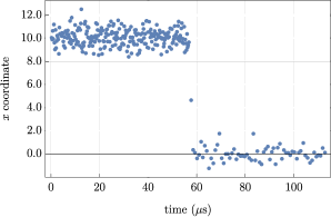
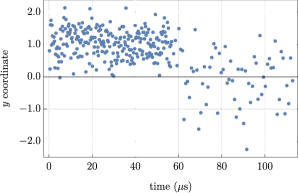
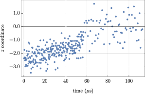
Figure 5: Averaged (over 200 subsequent firings) $x$, $y$, $z$ positions of the firing PMTs as a function of time (gravitino velocity $v_{E}$).

In Fig. 4 on the left we display the simulated number of detected photons as a function of time, taking into account all the assumptions listed above. As we can see the passage of gravitino can be clearly and unambiguously seen as being very different for the first 56 $\mu$s and the next 56 $\mu$s. No background or other particle can mimic such a signal.

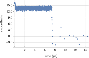
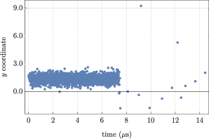
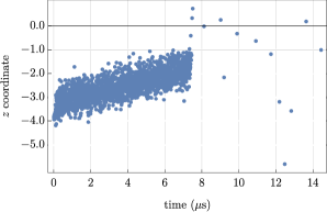
Figure 6: Averaged (over 200 subsequent firings) $x$, $y$, $z$ positions of the firing PMTs as a function of time (gravitino velocity $v_{S}$).

The track can then be reconstructed as follows. Since photons are emitted in all directions, to approximately reproduce the track it is reasonable to average over the positions of the firing photomultipliers – we have chosen to average over 200 consecutive firings. Fig. 5 presents the results of the simulation in an attempt to reconstruct the track. The horizontal axis is in microseconds and the vertical axis in meters showing on three figures average positions $x$, $y$ and $z$ of firing photomultipliers as a function of time of firing (they are the times of arrival, not the times of emission). As we can see comparing with (30), even in this unfavorable case (slow gravitino with smaller ratio signal/background than for the fast ones) we can approximately reproduce the track.

Next we discuss the case of fast gravitinos ($\beta=7.7\cdot 10^{-4}$). We start to count the time when the gravitino enters the ball, then, after it exits the ball (in 7 $\mu$s) we continue the simulation up to 14 $\mu$s to see the difference between signal plus background in the first 7 $\mu$s and only background (almost invisible in comparison) in the next 7 $\mu$s. In Fig. 4 on the right we display the simulated number of detected photons as a function of time. As we can see the passage of a gravitino can be even more clearly and unambiguously detected than before as being very different for the first 7 $\mu$s and the next 7 $\mu$s. We approximately reproduce the track after averaging, as before, over 200 consecutive firings and Fig. 6 presents the results of the simulation. When compared with (30) we see that the track can be well reproduced as a function of time with several meters of precision.

VII Final comments

Our calculation vividly illustrates why and how JUNO sits in a ‘sweet spot’ predestined to search for supermassive charged gravitinos. This is true not only for the most favorable case of galactic speeds $v\sim v_{S}$, for which the number of photons produced along the track is very large, but also for slow, ‘sun-bound’ gravitinos with $v\sim v_{E}$. As the simulations show, any passage of a gravitino, either slow or fast, close to the center or to the edge, should produce a clear and unmistakable signal if the electronics, triggering system and the software are set to take into account the possibility of long and continuous detection of photons over many microseconds. Finally, we would like to reiterate that the excitation cross sections for LAB reported in this work are conservative lower bounds, taking into account only the $S_{0}\rightarrow S_{1}$ excitation process. In subsequent paper, we shall consider other competing processes initiated by the passing gravitino, such as ionization or capture of an electron. The impact of these processes on the strength of the signal will be studied, improving the current lower bound.