The two-body problem in 2+1 spacetime dimensions with negative cosmological constant: two point particles

Abstract

We work towards the general solution of the two-body problem in 2+1-dimensional general relativity with a negative cosmological constant. The BTZ solutions corresponding to black holes, point particles and overspinning particles can be considered either as objects in their own right, or as the exterior solution of compact objects with a given mass $M$ and spin $J$, such as rotating fluid stars. We compare and contrast the metric approach to the group-theoretical one of characterising the BTZ solutions as identifications of 2+1-dimensional anti-de Sitter spacetime under an isometry. We then move on to the two-body problem. In this paper, we restrict the two objects to the point particle range $|J|-1\leq M<-|J|$, or their massless equivalents, obtained by an infinite boost. (Both anti-de Sitter space and massless particles have $M=-1$, $J=0$). We derive analytic expressions for the total mass $M_{\text{tot}}$ and spin $J_{\text{tot}}$ of the system in terms of the six gauge-invariant parameters of the two-particle system: the rest mass and spin of each object, and the impact parameter and energy of the orbit. Based on work of Holst and Matschull on the case of two massless, nonspinning particles, we conjecture that the black hole formation threshold is $M_{\text{tot}}=|J_{\text{tot}}|$. The threshold solutions are then extremal black holes. We determine when the global geometry is a black hole, an eternal binary system, or a closed universe.

I Introduction

General relativity in 2+1 spacetime dimensions appears dynamically trivial because in 2+1 dimensions the Weyl tensor is identically zero. This means that the full Riemann tensor is determined by the Ricci tensor, and so by the stress-energy tensor of the matter. Hence there are no gravitational waves, and the vacuum solution is locally unique: Minkowski in the absence of a cosmological constant $\Lambda$, de Sitter for $\Lambda>0$ and anti-de Sitter (from now on, adS3) for $\Lambda<0$.

However, it was noted by Deser, Jackiw and t’Hooft in 1984 DeserJackiwTHooft84 that even the general vacuum solution with $\Lambda=0$ is non-trivial if one allows for singularities representing point particles, which may be spinning. The global solution is then obtained by identifying Minkowski spacetime with itself under a non-trivial isometry for each particle. In the simplest case, this is a rotation by $2\pi-2\nu$, where the resulting spacetime can be thought of as Minkowski with a wedge of opening angle $2\nu$ removed and the two faces of the wedge identified. The dynamics of two or more interacting particles can then be dealt with in closed form using the algebra of such isometries.

In 1992, Bañados, Teitelboim and Zanelli BTZ92 (from now on, BTZ) noticed that 2+1 dimensional vacuum Einstein gravity with $\Lambda<0$ admits rotating black hole solutions parameterised by a mass $M$ and spin $J$ that share many features with the family of Kerr solutions in 3+1 dimensions. These can be found easily by solving an axistationary ansatz for the metric, but their existence had been overlooked because the metric has to be locally adS3. In fact, these metrics can be derived as non-trivial identifications of adS3 with itself BHTZ93 under the action of an isometry.

A key difference to black holes in 3+1 dimensions is the existence of a mass gap: while adS3 is given by the BTZ solution with parameters $M=-1$ and $J=0$, only the BTZ solutions with $M\geq 0$ and $|J|\leq M$ represent black holes. (These parameters are defined below). Solutions with all other real values of $M$ and $J$ have naked singularities and represent point particles ($|J|<-M$), similar to those for $\Lambda=0$ described in DeserJackiwTHooft84 , and overspinning particles ($|J|>|M|$).

Combining these two ideas suggests a research programme of completely solving the two-body problem in 2+1-dimensional gravity with $\Lambda<0$. A key insight is that the BTZ solutions are not only building blocks in their own right, but are also the exterior solutions of any compact object. By contrast, in 3+1 dimensions, the vacuum exterior spacetime of any spherical compact object is Schwarzschild, but the exterior of a non-spherical or rotating compact object is not in general Kerr, even the if the object is itself axistationary.

Because any vacuum spacetime with $\Lambda<0$ is locally isometric to adS3, the exterior spacetime of any compact object, like the vacuum BTZ solutions, must be an identification of adS3 with itself under an element of its isometry group. The basic idea is the following. Cover up the compact object with a world tube, remove the interior of the world tube, and make the resulting spacetime simply connected by making a suitable cut from the world tube to infinity. On this simply connected domain, the spacetime must now locally be adS3. To undo the cutting-open, we need to identify the two sides of the cut, and regularity then requires that the identification is via an isometry of adS3. It was shown in BHTZ93 that the gauge-invariant content of such an identification is a mass $M$ and spin $J$, characterising the BTZ spacetimes.

The isometry group of adS3 is usually obtained HawkingEllis by first characterising adS3 as a hyperboloid embedded in ${\mathbb{R}}^{(2,2)}$ endowed with a flat metric. Its symmetry group is then the subgroup of the isometry group of the embedding space that leaves the hyperboloid invariant, namely $SO(2,2)$. This approach gives us only the BTZ solutions for $M>|J|-1$. This includes all black hole solutions, but only a region of point particles and overspinning particles.

More explicitly, one can write the adS3 metric locally in terms of “cut and paste” coordinates $(\hat{t},\chi,\hat{\phi})$ in which the metric coefficients depend only on $\chi$. The BTZ metrics are then obtained by identifying $\hat{\phi}$ with a period smaller or larger than $2\pi$, and identifying $\hat{t}$ with a jump across the cut. The identifications not parameterised by an element of the isometry group are those in which the period is larger than $2\pi$ (rather than smaller), or the time jump larger than $2\pi$.

Spinning massless particles are obtained from point particles by applying an infinite boost and sending the mass to infinity simultaneously. They correspond to a non-trivial identification of adS3 across a null plane but have $M=-1$ and $J=0$ like adS3 itself.

Restricting ourselves to point particles with $|J|-1\leq M<-|J|$, or the vacuum exterior of compact objects in that parameter range, or the massless equivalents of point particles, we take an algebraic approach to the two-body problem in 2+1 dimensions with $\Lambda<0$ in which each object is obtained by an identification under isometry, and the resulting combined object is obtained by multiplying the two elements of the isometry group. We now summarise previous work using this approach.

Time-symmetric initial data for two massive point particles, two black holes, or one black hole and one massive point particle were constructed in Steif96 . Complete solutions describing two massless non-spinning particles without and with impact parameter were constructed in M99 ; HM99 , and two or more massive non-spinning particles colliding at one point in L16a ; L16b . With non-zero impact parameter, above a certain energy threshold the spacetime contains closed timelike curves (from now on, CTCs), in analogy with the Gott time machine Gott91 . However, if the boundary of the region of CTCs is considered as the physical singularity, this spacetime instead represents the creation of a rotating black hole from two particles HM99 .

In this paper, we generalise the algebraic approach of Steif96 ; M99 ; HM99 ; L16a ; L16b to computing the total mass and spin of the most general two-point-particle setup, allowing for arbitrary rest masses (including zero) and spins, and arbitrary center-of mass relative momentum and impact parameter. We do not, however, generalise the explicit spacetime constructions of M99 ; HM99 . Rather, we rely on the beautiful constructions in HM99 as providing a sufficiently general example to argue that a black hole forms from two point particles if and only if the total mass $M$ and spin $J$ obey the inequalities $M\geq 0$ and $|J|\leq M$ that characterise black holes.

We begin with parameter counting. Each compact object surrounded by vacuum has a rest mass (which can be zero), a spin (which can be zero), an initial position and an initial momentum. Hence the two-body initial data have 12 parameters. Six of these correspond to rotating, boosting and translating the two-body combined object, and so in the absence of any further objects in the universe they are pure gauge. The other six parameters of the initial data are gauge-invariant. One can take them to be the two rest masses, the two spins, the impact parameter measured in the rest frame, plus one more. For two massless nonspinning particles, we take this last parameter to be their energies in the rest frame (where they are equal). For two massive particles, we take it to be their total relative rapidity. For one massless and one massive particle we use the rapidity of the massive particle and the energy of the massless particle, both with respect to the rest frame.

In Sec. II, based on DeserJackiwTHooft84 ; BTZ92 ; BHTZ93 ; C95 ; MiskovicZanelli2009 , we review in explicit coordinates how metrics describing black holes, point particles and overspinning particles can be characterised as identifications of adS3. We discuss their spacetime structure and the role of closed timelike curves (CTCs).

In Sec. III, based on M99 ; HM99 ; BHTZ93 ; C95 ; MiskovicZanelli2009 , we review a group theoretical approach complementary to the metric approach of Sec. II, where adS3 is identified with the group manifold $SL(2,{\mathbb{R}})$ and the isometry group of adS3 is represented by $SL(2,{\mathbb{R}})\times SL(2,{\mathbb{R}})/{\mathbb{Z}}^{2}$ acting by conjugation, rather than by $SO(2,2)$ acting on ${\mathbb{R}}^{(2,2)}$. The two groups are related in Appendix A. We also point out that either group theory approach gives only BTZ solutions with $|J|<M+1$. Appendix B relates the coordinate and isometry group treatments of overspinning particles.

Appendix C considers the limit $\Lambda=0$ from both the coordinate and isometry group approach. We point out that spinning point particles can be defined in two ways, and have in fact been defined differently for $\Lambda=0$ and $\Lambda<0$ in the literature. We give a BTZ-like metric for point particles. We also give an exact expression for the total angular momentum of a pair of particles in the $\Lambda=0$ case that is missing from DeserJackiwTHooft84 .

In Sec. IV we review, based on M99 ; HM99 ; L16a ; L16b , how the isometries corresponding to massive non-spinning point particles (the “particle generators”) can be obtained from their geodesics. Massless particles are obtained in the limit of infinite boost and vanishing rest mass. In an alternative and more general approach, we obtain the generators for spinning massive point particles on arbitrary trajectories (for a single object in the universe, the trajectory is still pure gauge) by boosting and translating the generators of a single massive point particle sitting at the centre of the coordinate system. Again massless particles are obtained as a limit. The nonspinning massive particle case serves as check on this calculation.

In Sec. V we create systems of two objects by multiplying their generators. We explain in detail how the two different product orders correspond to different gauges, and how to define gauge-invariant physical quantities, such as the relative rapidity and the impact parameter of the particles in the rest frame of the collision. Appendix D gives a simple example of how the product generators define an effective particle and how the order of multiplication corresponds to a gauge choice.

In Sec. VI we obtain the total mass $M_{\text{tot}}$ and spin $J_{\text{tot}}$ of the two-particle system, based on the product generators. Motivated by the work of Holst and Matschull HM99 , we conjecture that a black hole (with mass $M_{\text{tot}}$ and spin $J_{\text{tot}}$) forms if and only $|J_{\text{tot}}|<M_{\text{tot}}$. Otherwise, they define an effective point particle or overspinning particle characterising the metric outside of both objects. If the two particles collide they could also form a single real particle. Appendix E summarises the work of Steif Steif96 on the time-symmetric case, which serves as a check on our results.

The algebraic shortcut approach for calculating $M_{\text{tot}}$ and spin $J_{\text{tot}}$ of a two-body system has previously been used in BS00 . There, they are expressed as functions of three parameters, but it remains unclear which three-dimensional subspace of the six-dimensional parameter space of the general two-body system is being examined.

Sec. VII contains our conclusions and a list of open questions.

II Metric description of adS3 and its identifications

II.1 AdS3

We consider the three-dimensional Einstein equations

$$G_{ab}+\Lambda\,g_{ab}=8\pi T_{ab}.$$ (1)

We use units where $c=G=1$. Note that in 2+1 Newton’s constant $G$ has units of 1/mass, so in such units mass is dimensionless and angular momentum has dimension of length.

We write the negative cosmological constant as

$$\Lambda=:-{1\over\ell^{2}}<0.$$ (2)

From now on and unless otherwise stated, we measure length and time in units of $\ell$, so that we can set $\ell=1$, and all quantities become dimensionless. $\ell$ can be reinstated from dimensional analysis, assuming that, still with $c=G=1$, $\ell$ itself and our coordinates $t$, $r$, $\rho$, $\chi$, $x_{i}$ and spin $J$ have dimension length, while the angle $\phi$ and mass $M$ are dimensionless.

Any solution of the Einstein equations (1) with $T_{ab}=0$ is locally isometric to adS3. This can be characterised as the hyperboloidal hypersurface

$$-x_{3}^{2}-x_{0}^{2}+x_{1}^{2}+x_{2}^{2}=-1,$$ (3)

embedded in ${\mathbb{R}}^{(2,2)}$ and endowed with the metric induced by the flat metric

$$ds^{2}=-dx_{3}^{2}-dx_{0}^{2}+dx_{1}^{2}+dx_{2}^{2}$$ (4)

on ${\mathbb{R}}^{(2,2)}$ HawkingEllis . The entire hypersurface (3) can be parameterised as

$$x_{3} = \cosh{{\chi}}\cos{t},$$ (5a)

$$x_{0} = \cosh{{\chi}}\sin{t},$$ (5b)

$$x_{1} = \sinh{{\chi}}\cos{\phi},$$ (5c)

$$x_{2} = \sinh{{\chi}}\sin{\phi},$$ (5d)

where the coordinate ranges are

$$0\leq{\chi}<\infty,\quad 0\leq{t}<2\pi,\quad 0\leq{\phi}<2\pi.$$ (6)

In these coordinates the induced metric becomes

$$ds^{2}=-\cosh^{2}{{\chi}}\,d{t}^{2}+d\chi^{2}+\sinh^{2}{{\chi}}\,d{\phi}^{2}.$$ (7)

The maximal analytic extension of adS3 is obtained by dropping the periodicity of ${t}$, thus taking the universal cover of the original, periodic, version. Each slice of constant $t$ is the hyperpolic 2-plane (from now on ${\mathbb{H}}^{2}$), which has constant negative curvature. For clarity, we will from now on refer to the periodic version as padS3 and the extended version as eadS3.

With the new radial coordinate

$$r:=\sinh{{\chi}}=\sqrt{x_{1}^{2}+x_{2}^{2}},$$ (8)

the metric of eadS3 can be written in the alternative form

$$ds^{2}=-\left(1+r^{2}\right)\,d{t}^{2}+\left(1+r^{2}\right)^{-1}\,dr^{2}+r^{2}\,d{\phi}^{2},$$ (9)

with coordinate ranges

$$0\leq r<\infty,\quad-\infty<{t}<\infty,\quad 0\leq{\phi}<2\pi.$$ (10)

A third useful form of the eadS3 metric is obtained by defining the radial coordinate

$$\rho:=\tanh{\chi\over 2}\qquad 0\leq\rho<1,$$ (11)

which implies

$$r={2\rho\over 1-\rho^{2}}.$$ (12)

The inverse can be written as

$$\rho={r\over\sqrt{r^{2}+1}+1}.$$ (13)

The metric becomes

$$ds^{2}={4\over(1-\rho^{2})^{2}}\left(-{(1+\rho^{2})^{2}\over 4}d{t}^{2}+d\rho^{2}+\rho^{2}\,d{\phi}^{2}\right).$$ (14)

In these coordinates, each ${\mathbb{H}}^{2}$ slice of constant ${t}$ is represented in conformally flat form, that is as the Poincaré disk. Timelike null infinity $r=\infty$ is now represented by the boundary $\rho=1$. The conformal diagram of eadS3 is a cylinder. In the resulting spacetime picture in coordinates $(t,\rho,\phi)$, lightcones are isotropic in $\phi$ but twice as wide at the centre $\rho=0$ as at the boundary $\rho=1$.

In a fourth coordinate system on eadS3, we introduce the tortoise radius

$$r_{*}:=\int{dr\over 1+r^{2}}=\tan^{-1}r,$$ (15)

with range

$$0\leq r_{*}<{\pi\over 2},$$ (16)

or equivalently

$$\sinh\chi=\tan r_{*}\quad\Leftrightarrow\quad\cosh\chi={1\over\cos r_{*}},$$ (17)

to write the metric (7) as

$$ds^{2}={1\over\cos^{2}r_{*}}\left(-dt^{2}+dr_{*}^{2}+\sin^{2}r_{*}\,d\phi^{2}\right).$$ (18)

The conformal spatial metric is now that of one half of a 2-sphere, representing the hyperbolic plane as the Klein disk. The lightcones are at 45 degrees in the radial direction, but are no longer isotropic.

Rotating the coordinates on the 2-sphere via

$$\sin r_{*}\cos\phi = \cos\theta,$$ (19)

$$\sin r_{*}\sin\phi = \sin\theta\cos\varphi,$$ (20)

$$\cos r_{*} = \sin\theta\sin\varphi,$$ (21)

(any two of these three equations are independent) gives

$$ds^{2}={1\over\sin^{2}\theta\sin^{2}\varphi}\left(-dt^{2}+d\theta^{2}+\sin^{2}\theta\,d\varphi^{2}\right).$$ (22)

Whereas the obvious family of null geodesics of (18), $r_{*}=t$ at constant $\phi$, form a null cone, all intersecting at the point $r_{*}=t=0$, the equally obvious family of null geodesics of (22), $\theta=t$ at constant $\varphi$, are parallel and meet only at the points $\theta=t=0$ and $\theta=t=\pi$ on the conformal boundary: they form the adS3 equivalent of a null plane HM99 .

II.2 BTZ black holes

The BTZ metric can be obtained by making an axistationary ansatz for the Einstein equations (1) in vacuum. It is BTZ92

$$ds^{2}=-f\,dt^{2}+f^{-1}\,dr^{2}+r^{2}(d\phi+\beta dt)^{2},$$ (23)

where

$$f:=-M+{r^{2}}+{J^{2}\over 4r^{2}},\qquad\beta:=-{J\over 2r^{2}}.$$ (24)

$M$ is dimensionless but $J$ has dimension length if we do not use units where $\ell=1$. Clearly the case $M=-1$ and $J=0$ is the eadS3 metric in the form (9). For any $M$ and $J$, the surfaces of constant $t$ are spacelike at sufficiently large $r$. The coordinates have the ranges (10). As a matter of convention, throughout this paper spacetime points with coordinates $(t,r,\phi)$ and $(t,r,\phi+2\pi)$ are always identified. We write such identifications as

$$(t,r,\phi)\sim(t,r,\phi+2\pi).$$ (25)

We note already that the same identification will look different in the coordinates ${\hat{\phi}}$ and ${\hat{t}}$ introduced later.

We focus first on the parameter range $M>0$ with $0\leq|J|\leq M$, for which the BTZ metric represents a black hole BTZ92 ; BHTZ93 ; C95 . We define the dimensionless parameters

$$\lambda_{+\pm}:=\sqrt{M\pm J}$$ (26)

and their linear combinations

$$s_{\pm}:={1\over 2}(\lambda_{++}\pm\lambda_{+-}).$$ (27)

We note for later the identities

$$M = s_{+}^{2}+s_{-}^{2},$$ (28)

$$J = 2s_{+}s_{-},$$ (29)

$$\sqrt{M^{2}-{J^{2}}} = s_{+}^{2}-s_{-}^{2}.$$ (30)

$s_{-}$ has the same sign as $J$, while $s_{+}>0$. The metric coefficient $f$ has zeros at $r^{2}=s_{\pm}^{2}$. We define $r_{+}:=s_{+}$ and $r_{-}:=|s_{-}|$. They obey $0\leq r_{-}\leq r_{+}$. The Killing vector $\partial/\partial t$ is timelike in the outer region $r>r_{+}$, spacelike in the middle region $r_{-}<r<r_{+}$ and again timelike in the inner region $r<r_{-}$.

As in the Kerr solution in 3+1 spacetime dimensions, Kruskal coordinates can be constructed to show that $r=r_{+}$ is an event horizon separating the outer and middle regions, and $r=r_{-}$ a Cauchy horizon separating the middle and inner regions BHTZ93 .

In the non-spinning case $J=0$, we have $r_{+}=\sqrt{M}$ and $r_{-}=0$, so the inner region does not exist. In the extremal case $M=|J|>0$, we have $r_{+}=r_{-}=\sqrt{M/2}$ and the middle region does not exist. We have referred here to “the” inner, middle and outer region, event horizon and Cauchy horizon, but in the maximally extended non-rotating black hole solutions there is a “left” as well as a “right” outer region, and in the spinning ones all these are repeated to the past and future, see BTZ92 or C95 for conformal diagrams.

In the subextremal case $|J|<M$, the BTZ black hole solution (23) can be locally identified with the hyperboloid (3), where formulas for the $x_{\mu}$ are given in the first three columns of Table 1 in terms of intermediate coordinates $({\hat{t}},{\chi},{\hat{\phi}})$. Those in turn are given in terms of the BTZ coordinates $(t,r,\phi)$ by

$$\chi = \begin{cases}\cosh^{-1}\sqrt{\alpha},&\text{outer region}\\ \sin^{-1}\sqrt{\alpha},&\text{middle region}\\ -\sinh^{-1}\sqrt{-\alpha},&\text{inner region}\end{cases},$$ (31a)

$${\hat{t}} = s_{+}t-s_{-}\phi,$$ (31b)

$${\hat{\phi}} = s_{+}\phi-s_{-}t,$$ (31c)

where we have introduced shorthand C95

$$\alpha:={r^{2}-r_{-}^{2}\over r_{+}^{2}-r_{-}^{2}}={{r^{2}}-s_{-}^{2}\over s_{+}^{2}-s_{-}^{2}}.$$ (32)

It is straightforward to verify that in each of the three regions the metric in $(t,r,\phi$) induced by (4) is indeed the BTZ metric (23). Note that the embeddings for the three regions of a black hole given in Table 1 differ from those given in BHTZ93 ; C95 by a gauge transformation. The gauge here has been chosen so that for nonspinning black holes the intersection of the plane $x_{3}=0$ with the hyperboloid is a moment of time symmetry, parameterised as $\hat{t}=0$, and that their generators (see below) then obey $u=v$. An explicit transformation from the BTZ metric to the adS3 metric (in the Poincaré coordinates) in the extremal case $|J|=M>0$ is given in BHTZ93 .

	outer region	middle region	inner region	point particle	overspinning particle
	$r_{+}<r<\infty$	$r_{-}<r<r_{+}$	$0<r<r_{-}$	$0<r<\infty$	$0<r<\infty$
	$0<{\chi}<\infty$	$0<{\chi}<{\pi\over 2}$	$\chi_{\rm bh}<{\chi}<0$	$\chi_{\rm pp}<{\chi}<\infty$	$\chi_{\rm os}<{\chi}<\infty$
$x_{3}$	$-\sinh{{\chi}}\,\sinh{\hat{t}}$	$-\cos{{\chi}}\,\cosh{\hat{t}}$	$-\cosh{{\chi}}\,\cosh{\hat{t}}$	$\cosh{{\chi}}\cos{\hat{t}}$	$-\cosh{{\chi}}\cosh{\tilde{\phi}}\sin{\tilde{t}}+\sinh{{\chi}}\sinh{\tilde{\phi}}\cos{\tilde{t}}$
$x_{0}$	$-\cosh{{\chi}}\,\cosh{\hat{\phi}}$	$-\sin{{\chi}}\,\cosh{\hat{\phi}}$	$\sinh{{\chi}}\,\sinh{\hat{\phi}}$	$\cosh{{\chi}}\sin{\hat{t}}$	$\cosh{{\chi}}\cosh{\tilde{\phi}}\cos{\tilde{t}}+\sinh{{\chi}}\sinh{\tilde{\phi}}\sin{\tilde{t}}$
$x_{1}$	$\cosh{{\chi}}\,\sinh{\hat{\phi}}$	$\sin{{\chi}}\,\sinh{\hat{\phi}}$	$-\sinh{{\chi}}\,\cosh{\hat{\phi}}$	$\sinh{{\chi}}\cos{\hat{\phi}}$	$-\cosh{{\chi}}\sinh{\tilde{\phi}}\cos{\tilde{t}}-\sinh{{\chi}}\cosh{\tilde{\phi}}\sin{\tilde{t}}$
$x_{2}$	$\sinh{{\chi}}\,\cosh{\hat{t}}$	$\cos{{\chi}}\,\sinh{\hat{t}}$	$\cosh{{\chi}}\,\sinh{\hat{t}}$	$\sinh{{\chi}}\sin{\hat{\phi}}$	$-\cosh{{\chi}}\sinh{\tilde{\phi}}\sin{\tilde{t}}+\sinh{{\chi}}\cosh{\tilde{\phi}}\cos{\tilde{t}}$

Table 1: Embedding of the BTZ solution into eadS3, in terms of $x^{\mu}$. The constants $\chi_{\text{bh}}$, $\chi_{\text{pp}}$ and $\chi_{\text{os}}$ are defined in (34), (44) and (50).

The induced metric in $({\hat{t}},{\chi},{\hat{\phi}})$ is

$$ds^{2} = -\sinh^{2}{{\chi}}\,d{\hat{t}}^{2}+d\chi^{2}+\cosh^{2}{{\chi}}\,d{\hat{\phi}}^{2},$$ (33a)

$$ds^{2} = \cos^{2}{{\chi}}\,d{\hat{t}}^{2}-d\chi^{2}+\sin^{2}{{\chi}}\,d{\hat{\phi}}^{2},$$ (33b)

$$ds^{2} = \cosh^{2}{{\chi}}\,d{\hat{t}}^{2}+d\chi^{2}-\sinh^{2}{{\chi}}\,d{\hat{\phi}}^{2}$$ (33c)

for the outer, middle and inner regions, respectively. These metrics are therefore alternative local forms of the adS3 metric. They are the only forms of the adS3 metric that are diagonal and depend on only one coordinate $\chi$, made unique by the choice $|g_{\chi\chi}|=1$.

We see that $\partial/\partial\hat{t}$ is the Killing generator of the event horizon, while $\partial/\partial\hat{\phi}$ is the Killing generator of the Cauchy horizon. In BTZ coordinates, the event horizon and Cauchy horizon generators are $\partial/\partial t+\Omega_{\pm}\partial/\partial\phi$ where $\Omega_{\pm}=J/(2r_{\pm}^{2})$, respectively.

The range of ${\chi}$ in each of the three regions is given in the second row of Table 1, with

$$\chi_{\rm bh}:=-\sinh^{-1}{|s_{-}|\over\left(M^{2}-{J^{2}}\right)^{1/4}}.$$ (34)

$\chi=\chi_{\rm bh}$ corresponds to $r=0$ in the inner patch.

From (31b,31c), the identification (25) in BTZ coordinates is equivalent to

$$({\hat{t}},{\chi},{\hat{\phi}})\sim({\hat{t}}-2\pi s_{-},{\chi},\hat{\phi}+2\pi s_{+}).$$ (35)

In particular, the angle $\hat{\phi}$ has period $2\pi s_{+}$ (with no particular significance of $s_{+}=1$), and the time coordinate ${\hat{t}}$ is identified with a jump

$$\Delta\hat{t}_{\rm bh}:=-2\pi s_{-},$$ (36)

which vanishes when $J=0$ and has the opposite sign from $J$. We shall refer to the intermediate coordinates $(\hat{t},\chi\,\hat{\phi})$ also as the cut-and-paste coordinates, in contrast to the BTZ coordinates $(t,r,\phi)$.

With the identification (35), the surfaces of constant $\hat{t}$ in the outer metric are wormholes, with a throat of circumference $2\pi r_{+}$ located at $\chi=0$. They can be interpreted as the Killing slicing of the two exterior regions of the Kruskal metric, with time going forwards in the right outer region, backwards in the left outer region, and each time slice going through the 2-surface $\chi=0$, equivalent to $x_{0}=x_{1}=0$, where the Killing horizon bifurcates.

II.3 Point particles

We next focus on the parameter range $M<0$, $|J|<-M$. Then the BTZ metric (23) has no horizons (zeros of $f$ for real $r$). Instead the BTZ solution for $M<0$ but $M\neq-1$ represents what one could either call a naked singularity BTZ92 or a point particle DeserJackiwTHooft92 . We define the two dimensionless parameters

$$\lambda_{-\pm}:=\sqrt{-M\pm J},$$ (37)

and their linear combinations

$$a_{\pm}:={1\over 2}(\lambda_{-+}\pm\lambda_{--})$$ (38)

as the equivalent of the BTZ black hole parameters $s_{\pm}$. They obey

$$-M = a_{+}^{2}+a_{-}^{2},$$ (39)

$$J = 2a_{+}a_{-},$$ (40)

$$\sqrt{M^{2}-{J^{2}}} = a_{+}^{2}-a_{-}^{2}.$$ (41)

$a_{-}$ has the same sign as $J$, while $a_{+}>0$.

The identification of the point particle BTZ solution with padS3 written as the hyperboloid (3) in ${\mathbb{R}}^{(2,2)}$ was found in MiskovicZanelli2009 . (However, MiskovicZanelli2009 restrict to $|J|\leq-M$ for $-1\leq M<0$ only. We do not see why this would be necessary.) This identification is given here in the second-last column of Table 1, with the intermediate coordinates now given in terms of the BTZ coordinates by

$${\chi} = \cosh^{-1}\sqrt{\alpha}$$ (42a)

$${\hat{t}} = a_{+}t+a_{-}\phi,$$ (42b)

$${\hat{\phi}} = a_{+}\phi+a_{-}{t}.$$ (42c)

Here $\alpha$ is defined by

$$\alpha={{r^{2}}+a_{+}^{2}\over a_{+}^{2}-a_{-}^{2}}.$$ (43)

[This is the same expression as (32) if we take into account that $s_{\pm}^{2}=-a_{\mp}^{2}$.] The range of ${\chi}$ is given in Table 1, with

$$\chi_{\rm pp}:=\cosh^{-1}{a_{+}\over\left(M^{2}-{J^{2}}\right)^{1/4}}.$$ (44)

$\chi=\chi_{\rm pp}$ corresponds to $r=0$. The expressions for the $x_{\mu}$ given in Table 1 in the point particle case are simply (5) with hats on, and so the induced metric in $({\hat{t}},{\chi},{\hat{\phi}})$ is

$$ds^{2}=-\cosh^{2}\chi\,d\hat{t}^{2}+d\chi^{2}+\sinh^{2}\chi\,d\hat{\phi}^{2},$$ (45)

The induced metric in $(t,r,\phi)$ is once again the BTZ metric (23).

The identification(25) is now equivalent to

$$({\hat{t}},{\chi},{\hat{\phi}})\sim({\hat{t}}+2\pi a_{-},{\chi},{\hat{\phi}}+2\pi a_{+}).$$ (46)

We can think of this as a wedge cut out with defect angle $2\nu>0$, or a wedge inserted with excess angle $2\nu<0$, where

$$\nu:=\pi\left(1-a_{+}\right),$$ (47)

and a time jump

$$\Delta{\hat{t}}_{\rm pp}:=2\pi a_{-},$$ (48)

which has the same sign as $J$, applied when identifying across the sides of the wedge. Hence we can think of the point particle geometry as eadS3 with a timelike conical singularity and time jump. The exception is $M=-1$ and $J=0$, which gives $a_{+}=1$ and $a_{-}=0$.

II.4 Overspinning particles

The $(J,M)$-plane is completed by two disjoint overspinning regions $|J|>|M|$. There are no horizons, and, as we will see below, if we restrict to $r\geq 0$ there are no closed timelike curves either. Hence we can consider the restriction most usefully as a kind of particle.

For clarity, in this paper we will call BTZ solutions with $M<0$, $|J|<-M$ “point particles”, and BTZ solutions with $|J|>|M|$ “overspinning particles”. Only the nonspinning particle solutions are unambiguously “point particles”, with a singular worldline at $r=\chi=0$, whereas in both spinning point particle and overspinning particle solutions a singular worldline at $\chi=0$ is surrounded by a world tube containing closed timelike curves whose outer boundary is at $r=0$, see the following Sec. II.5 for details. Therefore either all (spinning) point particle and overspinning particle solutions should be considered as “particles” or none. We have opted here for the former as the one more consistent with the established terminology in the literature.

To simplify notation, we now restrict to the case $J>|M|$. The case $J<-|M|$ can be obtained by flipping the signs of $\hat{\phi}$ and $J$, thus also replacing $\lambda_{\pm+}$ with $\lambda_{\pm-}$.

An identification of this class of solutions with padS3 in the form of (3) is given in the last column of Table 1, with

$$\chi = {1\over 2}\sinh^{-1}\left({2{r^{2}}-M\over\sqrt{{J^{2}}-M^{2}}}\right),$$ (49a)

$${\tilde{t}} = {\lambda_{-+}\over 2}(t+\phi),$$ (49b)

$${\tilde{\phi}} = {\lambda_{++}\over 2}\left(\phi-t\right).$$ (49c)

This is derived in Appendix B (using the methods of Sec. III below and Appendix A.) The value of $\chi$ corresponding to $r=0$ is

$$\chi_{\rm os}:={1\over 2}\sinh^{-1}\left({-M\over\sqrt{{J^{2}}-M^{2}}}\right).$$ (50)

The metric in $(t,r,\phi)$ is again the BTZ metric (23). The induced metric in intermediate coordinates $({\tilde{t}},\chi,{\tilde{\phi}})$ is

$$ds^{2} = -d{\tilde{t}}^{2}+d\chi^{2}+d{\tilde{\phi}}^{2}+2\sinh{2{\chi}}\,d{\tilde{\phi}}\,d{\tilde{t}}$$

$$= -\cosh^{2}{2{\chi}}\,d\tilde{t}^{2}+d\chi^{2}+\left(d\tilde{\phi}+\sinh{2{\chi}}\,d\tilde{t}\right)^{2}.$$

As a byproduct we have found yet another form of writing the metric of eadS3, see also BengtssonSandin2006 . Any parameterisation of the overspinning BTZ metric that represents it as an identification of adS3 with a shift in $\tilde{t}$ and a shift in $\tilde{\phi}$, where $\partial/\partial\tilde{t}$ and $\partial/\partial\tilde{\phi}$ are commuting Killing vectors of adS3, both before and after the identification, must be related to this one by a linear recombination of the coordinates $\tilde{t}$ and $\tilde{\phi}$ and a reparameterisation of the coordinate $\chi$. It is clear that no such reparameterisation can make the metric diagonal at the same time.

The identification (25) is equivalent to

$$({\tilde{t}},\chi,{\tilde{\phi}})\sim({\tilde{t}}+\pi\lambda_{-+},\chi,{\tilde{\phi}}+\pi\lambda_{++})$$ (52)

To make this look more like the point particle and black hole cases, we define the alternative cut-and-paste coordinates

$$\hat{t} := \tilde{t}-\tilde{\phi}=b_{+}t+b_{-}\phi,$$ (53)

$$\hat{\phi} := \tilde{t}+\tilde{\phi}=b_{+}\phi+b_{-}t,$$ (54)

where we have defined the shorthand parameters

$$b_{\pm}:={1\over 2}(\lambda_{-+}\pm\lambda_{++}).$$ (55)

The metric becomes

$$ds^{2}={1\over 2}\sinh 2\chi(-d\hat{t}^{2}+d\hat{\phi}^{2})+d\chi^{2}-d\hat{t}\,d\hat{\phi}$$ (56)

(yet another local coordinate system on adS3), and the identification is

$$({\hat{t}},\chi,{\hat{\phi}})\sim({\hat{t}}+2\pi b_{-},\chi,{\hat{\phi}}+2\pi b_{+}).$$ (57)

For the prototype overspinning particle $J=1$, $M=0$, this reduces $({\hat{t}},\chi,{\hat{\phi}})\sim({\hat{t}},\chi,{\hat{\phi}}+2\pi)$ just as for adS3 spacetime $M=-1$, $J=0$ and the prototype black hole $M=1$ and $J=0$.

II.5 Closed timelike curves

By replacing the coordinate $r$ with $R:=r^{2}$ in (23) we obtain

$$ds^{2}=\left(M-{R}\right)\,dt^{2}+{dR^{2}\over F}+R\,d\phi^{2}-J\,d\phi\,dt,$$ (58)

where

$$F:=4R^{2}-4MR+J^{2}=r^{2}f(r).$$ (59)

Hence we have an analytic continuation beyond $r=0$ to negative $R$. The metric (58) is regular, with regular inverse, except where $F=0$. These roots occur at

$$R_{\pm}:={M\pm\sqrt{M^{2}-J^{2}}\over 2}.$$ (60)

For point particles, $R=R_{+}=-a_{-}^{2}<0$ corresponds to the particle location $\chi=0$, which is a conical singularity. Therefore, the maximal analytic extension of the spacetime corresponds to $R_{+}<R<\infty$. The root $R=R_{-}$ of $F$ is not physical. For black holes or overspinning particles, the maximal analytic continuation of the spacetime corresponds to the range $-\infty<R<\infty$. For black holes, $R=-\infty$ is a segment of timelike infinity deep inside the black hole, see the Penrose diagram in BHTZ93 .

It is clear from the form (58) of the metric that there is a smooth closed timelike curve (CTC) through every point of the spacetime with $R<0$, namely the curve given by constant $t$ and $R$. Conversely, it was shown in BHTZ93 that if spacetime is restricted to $R>0$ there are no closed differentiable causal curves at all. We give this argument here for completeness. A differentiable curve $(t,r,\phi)(\tau)$ is causal if

$$-f\dot{t}^{2}+f^{-1}\dot{r}^{2}+r^{2}\left(\dot{\phi}+{J\over 2r^{2}}\dot{t}\right)^{2}\leq 0,$$ (61)

where a dot denotes $d/d\tau$. Causal curves that cross an event horizon or Cauchy horizon cannot cross it again and so cannot be closed. Hence it is sufficient to consider curves that remain in $f>0$ and curves that remain in $f<0$. In a spacetime region where $f>0$, we note that a closed differentiable curve must have one point where $\dot{t}=0$. But then there is a contradiction with (61) as long as $r^{2}>0$. Similarly, in a spacetime region where $f<0$, we note that a closed differentiable curve must have a point where $\dot{r}=0$ to obtain the same contradiction.

It was conjectured in BHTZ93 that any field theory matter falling into a BTZ black hole has divergent stress-energy at $r=0$ and so turns it into a genuine curvature singularity. Therefore it was proposed to exclude $r<0$ and consider $r=0$ as the true singularity, by extension even in the vacuum black hole case. Excluding the CTC region for point particles or overspinning particles can be justfied in the same way. However, if we think of the particle as corresponding to a singular stress-energy tensor with support on a world line, the point of view taken (for $\Lambda=0$) in DeserJackiwTHooft84 , that particle is at $\chi=0$ for point particles and at $\chi=-\infty$ for overspinning particles, not at $r=0$. A spinning “particle” at $r=0$ is really a brane, the point of view taken (for $\Lambda<0$) in MiskovicZanelli2009 . For the purpose of our calculations, it will not be necessary to take a view on this as long as the $r>0$ regions of the two particles never overlap (or at least not before before they have fallen into a black hole). It is worth stressing that the existence of CTCs is independent of the value of $\Lambda$, see also Appendix C.

III $SL(2,{\mathbb{R}})$ description of the isometries of padS3, and of the BTZ solutions

III.1 padS3 as a Lie group manifold

The hyperboloid (3) corresponding to the time-periodic spacetime padS3 can be mapped to the Lie group $SL(2,{\mathbb{R}})$ via the identification

$${\bf x}={x_{3}}I+{x_{0}}\gamma_{0}+{x_{1}}\gamma_{1}+{x_{2}}\gamma_{2},$$ (62)

where $I$ is the identity matrix and the $\gamma$-matrices are

$$\gamma_{0}=\left(\begin{array}[]{ c c }0&1\\ -1&0\end{array}\right),\>\gamma_{1}=\left(\begin{array}[]{ c c }0&1\\ 1&0\end{array}\right),\>\gamma_{2}=\left(\begin{array}[]{ c c }1&0\\ 0&-1\end{array}\right).$$ (63)

Together these form a basis of real $2\times 2$ matrices. The condition (3) is precisely the condition $\det{\bf x}=1$ for the matrix ${\bf x}$ to be an element of the group. The inverse of (62) is

$$x_{0} = -{1\over 2}\operatorname{tr}(\gamma_{0}{\bf x}),\quad x_{1}={1\over 2}\operatorname{tr}(\gamma_{1}{\bf x}),$$

$$x_{2} = {1\over 2}\operatorname{tr}(\gamma_{2}{\bf x}),\quad x_{3}={1\over 2}\operatorname{tr}({\bf x}).$$ (64)

We can parameterise the general element of $SL(2,R)$ as

$$g_{\text{gen}}(\zeta,\psi,\varphi) := \cosh\zeta\,(\cos\psi\,I+\sin\psi\,\gamma_{0})$$ (65)

$$+\sinh\zeta\,(\cos\varphi\,\gamma_{1}+\sin\varphi\,\gamma_{2}).$$

Taking the inverse of $g$ corresponds to changing the signs of the coefficients of $\gamma_{0}$, $\gamma_{1}$ and $\gamma_{2}$. Hence

$$g_{\text{gen}}(\zeta,\psi,\varphi)^{-1}=g_{\text{gen}}(-\zeta,-\psi,\varphi).$$ (66)

Note also that for $g,h\in SL(2,{\mathbb{R}})$, $\operatorname{tr}(g^{-1})=\operatorname{tr}g$ and $\operatorname{tr}gh=\operatorname{tr}hg$.

III.2 Isometries

In the representation of padS3 as $SL(2,{\mathbb{R}})$, any isometry $\phi$ can be represented as

$$\phi:\ {\bf x}\mapsto\tilde{\bf x}:=g^{-1}{\bf x}h,$$ (67)

where $g$ and $h$ are two elements of $SL(2,{\mathbb{R}})$, called the left and right generators of the isometry. $(g,h)$ and $(-g,-h)$ (and only those two pairs) represent the same isometry. We follow the convention of HM99 . (By contrast, C95 uses the convention $g{\bf x}h$.) The composition of isometries is then given by right matrix multiplication of the generators $(g,h)$, that is $\phi_{1}\circ\phi_{2}$ has generators $(g_{1}g_{2},h_{1}h_{2})$.

The isometry admits fixed points ${\bf x}=g^{-1}{\bf x}h$ if and only if the generators are in the same conjugacy class, that is, there exists an ${\bf x}$ such that

$$g={\bf x}h{\bf x}^{-1}.$$ (68)

In particular, if either $h=I$ or $g=I$ (but not both), $\phi$ is the left or right action and so acts freely (admits no fixed points). However, if any fixed points exist, the set of fixed points is precisely a geodesic HM99 , which can be interpreted as a generalised axis of rotation.

The isometry group of padS3 can also be represented as $SO(2,2)$ acting on ${\bf x}\in{\mathbb{R}}^{(2,2)}$ by matrix multiplication. See Appendix A for details.

III.3 Point particles, overspinning particles and black holes as isometries

As we have already seen, particles and black holes in adS3 can be represented by identifying the padS3 spacetime under a nontrivial isometry, that is

$$\psi:\ {\bf x}\sim u^{-1}{\bf x}v.$$ (69)

We can also look at the identification $\psi$ (considered as a physical particle or black hole) under the isometry $\phi$ (considered as a mere change of coordinate system that leaves the form of the metric invariant), that is $\tilde{\psi}:=\phi^{-1}\psi\phi$. In terms of the $SL(2,{\mathbb{R}})$ generators we have

$$g^{-1}{\bf x}h\sim g^{-1}u^{-1}{\bf x}vh=(g^{-1}ug)^{-1}(g^{-1}{\bf x}h)(h^{-1}vh)$$ (70)

or equivalently

$$\tilde{\bf x}\sim\tilde{u}^{-1}\tilde{\bf x}\tilde{v}$$ (71)

where the generators of the same isometry $\psi$, expressed in the new “coordinate system” $\tilde{\bf x}$ are

$$\tilde{u}:=g^{-1}ug,\qquad\tilde{v}:=h^{-1}vh.$$ (72)

This specifies how the generators $u$ and $v$ of the identification $\psi$ representing a physical particle transform under an independent isometry $\phi$ with generators $g$ and $h$ representing a coordinate change.

The identification of the spacetime with itself under the isometry $\psi$ is transitive. Hence with two objects (particle or black hole) we also have the identifications

$$\psi_{2}\circ\psi_{1}:\ {\bf x}\sim u_{2}^{-1}(u_{1}^{-1}{\bf x}v_{1})v_{2}=(u_{1}u_{2})^{-1}{\bf x}(v_{1}v_{2})$$ (73)

and

$$\psi_{1}\circ\psi_{2}:\ {\bf x}\sim u_{1}^{-1}(u_{2}^{-1}{\bf x}v_{2})v_{1}=(u_{2}u_{1})^{-1}{\bf x}(v_{2}v_{1})$$ (74)

We can think of these as the representation of an “effective particle”. We note that we can write

$$u_{1}u_{2}=u_{2}^{-1}(u_{2}u_{1})u_{2},\quad v_{1}v_{2}=v_{2}^{-1}(v_{2}v_{1})v_{2}.$$ (75)

Comparing (75) with (72), we see that the product particle generators taken in the two orders are related by the “coordinate transformation” (67) generated by $(g,h)=(u_{2},v_{2})$. Hence taking the product isometry in the two orders corresponds to the same effective particle in two different coordinate patches. See Appendix D for the visualisation of an example with $\Lambda=0$ that illustrates the effective particle in the two different gauges.

Throughout this paper, we use ${\bf x},{\bf y},{\bf z}$ for points in padS3, $u,v$ for left and right particle generators, and $g,h$ for left and right generators of a “coordinate change”, even though they are all elements of $SL(2,{\mathbb{R}})$.

What is the gauge-invariant information in a pair $(u,v)$ of generators? The eigenvalues of any matrix are invariant under conjugation, but since in $SL(2,{\mathbb{R}})$ the determinant (product of the eigenvalues) is always $1$ and there are only two such eigenvalues, two elements of $SL(2,{\mathbb{R}})$ are conjugate if and only if they have the same trace (sum of the eigenvalues). The product trace $\operatorname{tr}(u_{1}u_{2})$ is also gauge-invariant, and independent of the product order. We will see that the traces of particle generators encode the rest mass and spin of the particle, and so the traces of the product generators (in either order) encode the rest mass and spin of the effective particle. No other gauge-invariant quantities can be constructed from $(u,v)$.

For two spacetime points ${\bf x}$ and ${\bf y}$ in adS3 linked by a geodesic, the geodesic distance $d({\bf x},{\bf y})$ between them is given by

$${1\over 2}\operatorname{tr}\left({\bf x}^{-1}{\bf y}\right)=\begin{cases}\cos d({\bf x},{\bf y})&\hbox{spacelike,}\\ \cosh d({\bf x},{\bf y})&\hbox{timelike,}\\ 1&\hbox{null separated.}\end{cases}$$ (76)

This is easily verified by considering simple cases and noting that both the left-hand side and the right-hand side of this equation are gauge-invariant.

III.4 BTZ generators

The isometry $\psi$ of the BTZ black hole solutions is of the form (69) with generators

$$\left.\begin{aligned} u_{\rm bh}\\ v_{\rm bh}\end{aligned}\right\} = -\cosh\beta_{\mp}\,I-\sinh\beta_{\mp}\,\gamma_{2}$$ (77)

$$= -\cosh\left(\pi\sqrt{M\mp J}\right)\,I-\sinh\left(\dots\right)\,\gamma_{2}$$

for $M\geq 0$, $|J|\leq M$. We have made an arbitrary choice of overall sign, such that the generators of padS3 are $I$ [compare the limit $M=-1$, $J=0$ of (79) below.] To avoid writing factors of $\pi$, we have introduced the shorthands

$$\beta_{\pm}:=\pi\lambda_{+\pm}.$$ (78)

From Table 1 and (31b-31c) we can verify explicitly that (69) with (77) acts on the outer, middle and inner region of the BTZ black hole spacetime in the same way as $\phi\to\phi+2\pi$ in the BTZ coordinates $(t,r,\phi)$. However, the $SL(2,{\mathbb{R}})$ picture covers the identifications in all three regions at once.

The isometry $\psi$ of the BTZ spinning point particle solutions is of the form (69) with generators

$$\left.\begin{aligned} u_{\rm pp}\\ v_{\rm pp}\end{aligned}\right\} = \cos\nu_{\mp}\,I+\sin\nu_{\mp}\,\gamma_{0}$$ (79)

$$= -\cos\left(\pi\sqrt{-M\pm J}\right)\,I+\sin\left(\dots\right)\,\gamma_{0}.$$

To avoid writing factors of $\pi$, we have introduced the shorthands

$$\nu_{\pm}:=\pi(1-\lambda_{-\mp})=\nu\pm{\Delta\hat{t}_{\rm pp}\over 2}$$ (80)

We can again verify explicitly that this acts on the BTZ black hole spacetime in the same way as $\phi\to\phi+2\pi$ in the BTZ coordinates.

The BTZ generators for overspinning particles with $J>|M|$ are

$$u_{J>|M|}=u_{\rm pp},\quad v_{J>|M|}=v_{\rm bh},$$ (81)

and for $J<|M|$ they are

$$u_{J>|M|}=u_{\rm bh},\quad v_{J>|M|}=v_{\rm pp}.$$ (82)

The coordinate formulas in Sec. II.4 were actually found by the methods of Appendix B from the generators (81,82).

Put differently, in all parts of the $(J,M)$-plane, we choose $u=u_{\rm bh}$ if $M-J>0$ and $u=u_{\rm pp}$ if $M-J<0$, and we choose $v=v_{\rm bh}$ if $M+J>0$ and $v=v_{\rm pp}$ if $M+J<0$.

The generators of the $M=J=0$ spacetime appear to be $u=v=-I$, but this is not the correct limit. From (35), we see that as $s_{+}\to 0$, the fundamental domain between the two surfaces $\hat{\phi}=0$ and $\hat{\phi}=2\pi s_{+}$ disappears. The correct way of taking the limit is to apply a boost at the same time BHTZ93 . The two identification surfaces then do not approach each other uniformly as the limit is taken, but touch only at one end (infinity) while staying apart at the other end.

III.5 $M$ and $J$ from the traces of the isometry generators

The traces of the generators are related to each other in the four segments of the $(J,M)$-plane by analytic continuation. We have

$$Tu = -\cosh\pi\sqrt{M-J}=-\cos\pi\sqrt{-M+J},$$ (83a)

$$Tv = -\cosh\pi\sqrt{M+J}=-\cos\pi\sqrt{-M-J}$$ (83b)

for the BTZ generators everywhere in the $(J,M)$ plane. By contrast, there is no direct analytic continuation of the entire generators. To obtain one, one would have to apply a gauge transformation to the generators in order to transform a curve in $SL(2,{\mathbb{R}})\times SL(2,{\mathbb{R}})$ of generators that turns a corner at $J=\pm M$, with either $u=-I$ or $v=-I$, into a smooth one.

We define the function

$${\cal T}(Q):=-\cosh\pi\sqrt{Q}=-\cos\pi\sqrt{-Q}$$ (84)

which is complex-analytic in the entire $Q$ plane, and in particular is real-valued and real-analytic on the real line $-\infty<Q<\infty$. For $-\infty<T\leq 1$, ${\cal T}(Q)$ has the real analytic inverse

$${\cal Q}(T):={[\cosh^{-1}(-T)]^{2}\over\pi^{2}}=-{[\cos^{-1}(-T)]^{2}\over\pi^{2}}.$$ (85)

The function ${\cal Q}(T)$ is shown in Fig. 1. We can then write

$$Tu = {\cal T}(M-J),$$ (86a)

$$Tv = {\cal T}(M+J)$$ (86b)

for all real values of $M$ and $J$, or equivalently

$$M-J = {\cal Q}(Tu),$$ (87a)

$$M+J = {\cal Q}(Tv).$$ (87b)

This bijection between $(u,v)$ and $(J,M)$ is defined only for $Tu,Tv\leq 1$, and $|J|\leq M+1$. Fig. 2 shows the regions in the $(J,M)$ plane representing black holes, point particles and overspinning particles, and where these can be represented using the group theory approach.

Figure 1: A plot of ${\cal Q}(T)$. It is defined for $T\leq 1$. Note ${\cal Q}(-1)=0$, ${\cal Q}(0)=-1/4$ and ${\cal Q}(1)=-1$.

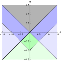
Figure 2: A plot of the $(J,M)$ plane, showing the black hole region (black), region of point particles that can be represented using the $SL(2,{\mathbb{R}})$ approach (dark green) and cannot (light green), and regions of overspinning particles that can be represented using the $SL(2,{\mathbb{R}})$ approach (dark blue) and cannot (light blue). The two objects considered in this paper take parameters in the dark green region.

III.6 Applicability of the isometry group approach

We have seen that the approach of identifying padS3 or eadS3 under an isometry of padS3 covers all the BTZ black hole solutions, but point particles and overspinning particles only for $|J|<M+1$. In other words, we can only represent point particles in parameter region

$$-1+|J|<M<-|J|$$ (88)

(the dark green region in Fig. 2), and overspinning particles in the parameter region

$$-|M|<|J|<-1+M$$ (89)

consisting of two disjoint parts $J>0$ and $J<0$ (the dark blue region in Fig. 2). The BTZ solutions we miss are those that require identifications

$$(\hat{t},\chi,\hat{\phi})\sim(\hat{t}+\Delta\hat{t},\chi,\hat{\phi}+\Delta\hat{\phi})$$ (90)

with $|\Delta\hat{t}|>2\pi$ or $\Delta\hat{\phi}>2\pi$ or both, whereas both have period $2\pi$ in the metric (45) of padS3. Unwinding $\hat{t}$ gives rise to the eadS3 solution, but already we are not aware of a parameterisation of the isometry group of eadS3 that allows easy multiplication. Further unwinding $\hat{\phi}$ produces a spacetime that we may call uadS3, with a branch point at $\chi=0$. Its isometry group is presumably the universal cover of $SL(2,{\mathbb{R}})\times SL(2,{\mathbb{R}})$, but this is not a matrix group and so does not allow for easy multiplication.

At this point, we seem to be facing a technical obstacle that we have not managed to overcome. However, one may wonder if the the BTZ solutions we are missing actually arise as exteriors of physical compact objects.

This question is suggested by the example of fluid stars. All rigidly rotating perfect fluid stars, for arbitrary equation of state, have been constructed explicitly in 2+1rotstars , building on the earlier work Cataldo . (The construction is formally for barotropic equations of state, but in an axistationary solution, where everything depends only on $r$, a stratified equation of state cannot be distinguished from a barotropic one). For any barotropic equation of state that has sound speed no greater than the speed of light and admits solutions with finite mass, stars with exterior metrics of all three types (point particle, black hole and overspinning particle) exist. These precisely fill the region $|J|<M+1$ with $M>-1$ of BTZ parameter space that is characterised by isometries of padS3.

IV A spinning point particle on an arbitrary trajectory

IV.1 Timelike geodesics

The world line $r=0$ of a point particle given by the BTZ metric corresponds to the world tube $\chi=\chi_{\text{pp}}$ surrounding the geodesic $\chi=0$ in the metric (45). More generally, the world line of any freely falling compact object corresponds to a world tube surrounding a geodesic of eads3. Hence we begin by calculating the timelike geodesics of eadS3.

Since the metric ($\ref{adS3metric})$ is independent of both $\phi$ and $t$, both $\partial_{t}$ and $\partial_{\phi}$ are Killing vectors, giving rise to the conserved energy (per rest mass)

$$E:=-u_{a}(\partial/\partial_{t})^{a}=\cosh^{2}\chi\ \dot{t}$$ (91)

and angular momentum (per rest mass)

$$L:=u_{a}(\partial/\partial_{\phi})^{a}=\sinh^{2}\chi\ \dot{\phi}.$$ (92)

Here a dot denotes $d/d\tau$ and $\tau$ is the proper time. The normalisation condition $u_{a}u^{a}=-1$ becomes a nonlinear first-order differential equation for $\chi(\tau)$, namely

$$\dot{\chi}^{2}+\frac{L^{2}}{\sinh^{2}\chi}-\frac{E^{2}}{\cosh^{2}\chi}=-1.$$ (93)

In the coordinate $r$ defined in Eq. (8) this becomes

$$\dot{r}^{2}=E^{2}-\left(1+{1\over r^{2}}\right)L^{2}-(1+r^{2}).$$ (94)

Taking the square root, we obtain a separable ODE that can be integrated in closed form to obtain

$$\chi(\tau)=\sinh^{-1}\left(\sqrt{C-D\cos 2\tau}\right),$$ (95)

where we have defined the temporary shorthands

$$C:=\frac{E^{2}-L^{2}-1}{2},\qquad D:=\sqrt{C^{2}-L^{2}}.$$ (96)

Without loss of generality, we have fixed the origin of $\tau$ so that the closest approach to the “central” world line $\chi=0$ is at $\tau=n\pi$ for integer $n$. The proper distance at these moments, measured along surfaces of constant $t$ (and in units of $\ell$) is

$$\delta:=\sinh^{-1}\sqrt{C-D}.$$ (97)

By integrating the definitions of $E$ and $L$ we then obtain $t(\tau)$ and $\phi(\tau)$.

We define the Lorentz factor $\Gamma$, rapidity $\gamma$ and 2-velocity $v$ of the geodesic with tangent vector $u^{a}$, with respect to the observers $n^{a}$ normal to the slices of constant $t$, by

$$\Gamma:=\cosh\gamma:={1\over\sqrt{1-v^{2}}}:=-u^{a}n_{a},$$ (98)

where $u_{a}u^{a}=n_{a}n^{a}=-1$. We note for later use that $v=\tanh\gamma$. With $n_{a}=-\cosh\chi\,(dt)_{a}$, we find

$$\Gamma(\tau)={E\over\cosh\chi(\tau)}.$$ (99)

We now define the constant parameter

$$z:=\gamma(0)=\cosh^{-1}\left({E\over\cosh\delta}\right).$$ (100)

In terms of the parameters $\delta$ and $z$, we then have

$$E=\cosh z\cosh\delta,\quad L=\sinh z\sinh\delta,$$ (101)

and the geodesics are given by

$$\chi(\tau) = \sinh^{-1}\sqrt{\sin^{2}\tau\sinh^{2}z+\cos^{2}\tau\sinh^{2}\delta},$$ (102a)

$$t(\tau) = \tan^{-1}\left({\cosh z\tan\tau\over\cosh\delta}\right)+t_{0},$$ (102b)

$$\phi(\tau) = \tan^{-1}\left({\sinh z\tan\tau\over\sinh\delta}\right)+\phi_{0},$$ (102c)

where $t_{0}$ and $\phi_{0}$ are arbitrary integration constants. We can now allow both $z$ and $\delta$ to have either sign. If we think about geodesics in terms of initial data at, say, $t=0$, the free data are the initial position and 2-velocity, requiring $4$ parameters. These can be mapped to our parameters $t_{0}$, $\phi_{0}$, $\delta$ and $z$, up to $t_{0}\to t_{0}+2n\pi$.

$\chi(\tau)$ is periodic with period $\pi$, and take values between $|\delta|$ and $|z|$, either of which could be the larger one of the two. We interpret the inverse $\tan^{-1}$ so that $t(\tau)$ always increases monotonically, and $\phi(\tau)$ increases (decreases) monotonically if $\delta$ and $z$ have the same (opposite) sign. When $\tau$ has increased by $2\pi$, $t$ has increased by $2\pi$, $\phi$ has changed by $2\pi$ or $-2\pi$, and $\chi$ has gone through two periods.

Looking back, we see that (94) is formally identical to the effective radial equation of motion of a Newtonian particle with energy per mass $C$, angular momentum per mass $L$, and an attractive central force per mass equal to the radius $r$ (like the force of a spring). Hence it is not surprising that in terms of $x_{1}$ and $x_{2}$ the timelike geodesics are the ellipses

$$\left({x_{1}\over\sinh z}\right)^{2}+\left({x_{2}\over\sinh\delta}\right)^{2}=1.$$ (103)

The relative sign of $z$ and $\delta$ determines the direction of the orbit. In the special cases $\delta=\pm z$ the orbits become circular. The timelike geodesic $\chi=0$ that appears to be at the centre of each of these ellipses is not privileged physically. Rather, as the background spacetime is maximally symmetric, any one timelike geodesic can be transformed into $\chi=0$ by an isometry, and this will transform all other timelike geodesics into ellipses about this new centre.

Because all geodesics have the same period $2\pi$ in $t$ (and in $\tau$), any two timelike geodesics that intersect once do so an infinite number of times at coordinate time intervals $\Delta t=\pi$ and proper time intervals $\Delta\tau=\pi$, irrespective of their relative boost at the points of intersection. This periodicity also relates the timelike geodesics of padS3 and eadS3.

IV.2 Null geodesics

To find null geodesics as a limit of our timelike geodesics, we take the boost $z$ to infinity while also rescaling the proper time $\tau$ by an infinite factor. Reparameterising $\tau$ as

$$\lambda:=\tau\cosh z$$ (104)

and taking the limit $z\to\infty$, we obtain

$$\chi(\lambda) = \sinh^{-1}\sqrt{\lambda^{2}+\sinh^{2}\delta},$$ (105a)

$$t(\lambda) = \tan^{-1}\left({\lambda\over\cosh\delta}\right)+t_{0},$$ (105b)

$$\phi(\lambda) = \tan^{-1}\left({\lambda\over\sinh\delta}\right)+\phi_{0}.$$ (105c)

Null geodesics can of course also be found directly from (93) with the right-hand side set to $0$ instead of $-1$. The affine parameter $\lambda$ is defined only up to an affine transformation. With (104) we have normalised $\lambda$ so that $dt/d\lambda=1/\cosh\delta$ at $\lambda=0$, which is the moment of closest approach to $\chi=0$. In contrast to the timelike case, for $-\infty<\lambda<\infty$, each null geodesic crosses eadS3 exactly once, entering and leaving through the timelike infinity at $t=t_{0}\mp\pi/2$, $\chi=\infty$, $\phi=\phi_{0}\mp\pi/2$.

IV.3 Massive non-spinning particles

An elegant way of computing isometry generators that leave a given geodesic invariant was given in HM99 . This can be used to find the generators of any nonspinning point particle. It is easily verified that if we take any two points ${\bf y}$ and ${\bf z}$ and define $u={\bf z}{\bf y}^{-1}$ and $v={\bf y}^{-1}{\bf z}$, then ${\bf x}=u^{-1}{\bf x}v$ is obeyed both for ${\bf x}={\bf y}$ and for ${\bf x}={\bf z}$. But locally any two points ${\bf y}$ and ${\bf z}$ define a unique geodesic ${\bf x}(\tau)$ through them. Finally, it can be shown that the fixed points of an isometry of padS3, if there are any, must form a geodesic HM99 . Combining these two facts, we must have that ${\bf x}(\tau)=u^{-1}{\bf x}(\tau)v$ for all points on the geodesic. Hence $u$ and $v$ obtained from any two points ${\bf y}={\bf x}(\tau_{\bf y})$ and ${\bf z}={\bf x}(\tau_{\bf z})$ on a geodesic are the generators of an isometry that leaves precisely this geodesic invariant. It is clear that the generator can depend only on $\nu:=\tau_{\bf z}-\tau_{\bf y}$.

The general timelike geodesic (102a-102c) in $SL(2,{\mathbb{R}})$ notation, using (62) and (5), is

$${\bf x}(\tau) = (\cos t_{0}\cosh\delta\cos\tau-\sin t_{0}\cosh z\sin\tau)\,I$$

$$+ (\cos t_{0}\cosh z\sin\tau+\sin t_{0}\cosh\delta\cos\tau)\,\gamma_{0}$$

$$+ (\cos\phi_{0}\sinh\delta\cos\tau+\sin\phi_{0}\sinh z\sin\tau)\,\gamma_{1}$$

$$+ (\cos\phi_{0}\sinh z\sin\tau-\sin\phi_{0}\sinh\delta\cos\tau)\,\gamma_{2},$$

where $\tau$ is proper time. The generators in terms of $\nu$, $\delta$, $z$, $t_{0}$ and $\phi_{0}$ become

$$\left.\begin{aligned} u\\ v\end{aligned}\right\} = \cos\nu\,I+\sin\nu\Bigl{\{}\cosh z_{\pm}\,\gamma_{0}$$ (107)

$$+\sinh z_{\pm}\left[-\sin\phi_{\pm}\,\gamma_{1}+\cos\phi_{\pm}\,\gamma_{2}\right]\Bigr{\}},$$

where we have defined the shorthands

$$z_{\pm}:=z\pm\delta,\qquad\phi_{\pm}:=\phi_{0}\pm t_{0}.$$ (108)

They obey the identities

$$u(t_{0},\phi_{0},z,\delta,\nu)=v(-t_{0},\phi_{0},z,-\delta,\nu)$$ (109)

relating the left and right generator, and the rotation symmetry

$$u(t_{0},\phi_{0}+\pi,z,\delta,\nu)=u(t_{0},\phi_{0},-z,-\delta,\nu)$$ (110)

and similarly for $v$. The latter symmetry is intuitive: reversing both boost and impact parameter is equivalent to a rotation by $\pi$. Note also that the geodesic in $SL(2,{\mathbb{R}})$ notation and the particle generators are regular as $\delta\to 0$, whereas the expressions for $t$, $\chi$ and $\phi$ are not, due to the coordinate singularity of the polar coordinates $(\chi,\phi)$ at $\chi=0$.

The generators for a particle sitting still at $\chi=0$, with $\delta=z=0$, are simply

$$u=v=\cos\nu\,I+\sin\nu\,\gamma_{0},$$ (111)

which agrees with the BTZ generators (79) for zero spin. We read off

$$Tu=Tv=\cos\nu,$$ (112)

and as the trace is invariant under conjugation, this expression is invariant under the isometries that map one timelike geodesic to another, and so it must be related to the rest mass of any nonspinning particle, independently of location and velocity. If we combine two massive nonspinning particles on the same geodesic (characterized by $\delta$, $z$, and $\phi_{0}$) by multiplying their generators, we find that $(u_{1}u_{2},v_{1}v_{2})$ describe another particle on this geodesic, with mass $\nu_{1}+\nu_{2}$. So $\nu$ is proportional to the locally measured particle mass. The factor of proportionality is obtained by directly solving the Einstein equations with the distributional stress-energy tensor

$$T_{ab}=mu^{a}u^{b}\delta({\bf x}),$$ (113)

which makes sense in 2+1 dimensions (only). The result is $\nu=4\pi m$ DeserJackiwTHooft84 , see also Appendix C. Because the source is infinitesimally small, this is independent of $\Lambda$.

IV.4 Massless non-spinning particles

To obtain the massless limit of the massive particle generators, we let $z\to\infty$ at the same time as $\nu\to 0$ such that

$$\lim_{\nu\to 0}\nu\cosh z=:{W}$$ (114)

is finite. We obtain

$$\left.\begin{aligned} u\\ v\end{aligned}\right\}=I+{W}e^{\mp\delta}\left[\gamma_{0}-\sin\phi_{\pm}\,\gamma_{1}+\cos\phi_{\pm}\,\gamma_{2}\right].$$ (115)

Equivalently, we can repeat the construction of the particle generators from the geodesic it is on. The null geodesics (105a-105c) in $SL(2,{\mathbb{R}})$ notation are

$${\bf x}(\lambda) = (\cos t_{0}\cosh\delta+\lambda\sin t_{0})\,I$$ (116)

$$+ (\sin t_{0}\cosh\delta+\lambda\cos t_{0})\,\gamma_{0}$$

$$+ (\cos\phi_{0}\sinh\delta-\lambda\sin\phi_{0})\gamma_{1}$$

$$+ (\sin\phi_{0}\sinh\delta+\lambda\cos\phi_{0})\gamma_{2}.$$

We find (115) again, with ${W}:=\lambda_{\bf z}-\lambda_{\bf y}$. Putting two massless particles with energies ${W}_{1}$ and ${W}_{2}$ on the same geodesic, the product of their generators has $W={W}_{1}+{W}_{2}$, so $W$ is proportional to the particle energy, see also the end of Sec. VI.3 below for the relation between $W$ and energy.

IV.5 Massive spinning particle

The approach starting from a geodesic cannot be extended to spinning particles, as their symmetry identifies any point on the particle world line with another one, shifted in time. However, we can obtain the generators for a massive spinning particle by boosting and displacing the BTZ solution. The 5-parameter family of isometries (67) with generators

$$\left.\begin{aligned} g\\ h\end{aligned}\right\}:=g_{\text{gen}}\left({z_{\mp}\over 2},\psi,\phi_{\pm}+\psi\right),$$ (117)

where $g_{\text{gen}}$ was defined in (65) and $\phi_{\pm}$ was defined in (108), is the most general one (out of the 6-dimensional group of all isometries) which maps the timelike “central” geodesic $\chi=0$ of the padS3 metric (7), represented in $SL(2,{\mathbb{R}})$ notation as

$${\bf x}_{c}=\cos(t_{0}+\tau)\,I+\sin(t_{0}+\tau)\,\gamma_{0},$$ (118)

to the geodesic (102a-102c), represented as (IV.3). We have already parameterised it so that it maps the generators (79) of the nonspinning BTZ point particle to (107) via the action (72).

This 5-parameter family is periodic with period $2\pi$ in $\phi_{\pm}$ and $\psi$. Moreover, shifting $\psi$ by $\pi$ changes only the overall sign of $g$ and $h$, and so corresponds to the same isometry. Changing the signs of both $z$ and $\delta$ is equivalent to shifting either $t_{0}$ or $\phi_{0}$ by $\pi$, as was the case for non-spinning particles. Both $g$ and $h$ have a left factor $\cos\psi\,I+\sin\psi\,\gamma_{0}$ that corresponds to a rotation by $2\psi$ in the $x_{1}x_{2}$ plane (which leaves the particle trajectory unchanged), applied before any boost and displacement.

Hence we define the generators of a boosted and displaced spinning point particle by (72) with (117), obtaining

$$\left.\begin{aligned} u\\ v\end{aligned}\right\} = \cos\nu_{\mp}\,I+\sin\nu_{\mp}\,\Bigl{\{}\cosh z_{\mp}\,\gamma_{0}$$

$$+\sinh z_{\mp}\,\left[-\sin\phi_{\pm}\,\gamma_{1}+\cos\phi_{\pm}\,\gamma_{2}\right]\Bigr{\}}.$$

The value of $\psi$ does not affect the generators. As expected, these generators map the geodesic (IV.3) to itself but with a time jump $\tau\to\tau+2\pi a_{-}$, compare (48). In the nonspinning case, we have $\nu_{+}=\nu_{-}=\nu$, and and (IV.5) reduces to (107).

IV.6 Massless spinning particle

We reparameterise

$$M=-1+{2W\over\pi\cosh z},\quad J={2U\over\pi\cosh z}$$ (120)

The condition $|J|<M+1$ for the particle to be representable as an isometry of padS3 is equivalent to $0<W<|U|$ (energy dominates spin).

We now define the massless limit of (IV.5) by letting $z\to\infty$ while keeping $W$, $U$ and $\delta$ fixed. The resulting generators are

$$\left.\begin{aligned} u\\ v\end{aligned}\right\} = I+e^{\mp\delta}(W\mp U)\bigl{[}\gamma_{0}$$ (121)

$$-\sin\phi_{\pm}\gamma_{1}+\cos\phi_{\pm}\gamma_{2}\bigr{]}.$$

We recover the nonspinning case (115) by setting $U=0$. Both $W$ and $U$ are additive if we place two massless particles on the same orbit, so are proportional to the particle energy and spin.

The generator traces for a massless spinning particle are $Tu=Tv=1$, as for the adS3 solution itself, so in contrast to the massive spinning particles these are not BTZ solutions. It is clear that they cannot be, as the BTZ solutions are by ansatz axisymmetric and stationary, while the massless particle solutions are neither: the particle crosses eadS3 at a specific time and in a specific direction, which breaks these symmetries.

The fact that only the generator traces are gauge-invariant, but they are both 1, also suggests a single massless particle cannot be distinguished from vacuum adS3 in a gauge-indepenent way. We can make a gauge transformation from (121) to

$$\left.\begin{aligned} \tilde{u}\\ \tilde{v}\end{aligned}\right\}=I+e^{\alpha_{\mp}}(W\mp U)(\gamma_{0}+\gamma_{2}),$$ (122)

for two arbitrary (real and finite) gauge parameters $\alpha_{\mp}$. Hence not only the orbital parameters $\delta$, $\phi_{0}$ and $t_{0}$ are pure gauge, as one would expect, but so are $W\pm U$, up to the fact they do not vanish and their sign.

What is the identification isometry parameterised by (121)? The 1-parameter family of null geodesics (116), with $\phi_{0}$ and $t_{0}$ fixed, $-\infty<\delta<\infty$ labelling the geodesics, and $\lambda$ the affine parameter along thm, form a null plane. This is most easily seen in ${\mathbb{R}}^{(2,2)}$, where the family with, for simplicity, $\phi_{0}=t_{0}=0$ is given by

$$x^{\mu}=(\cosh\delta,\lambda,\sinh\delta,\lambda).$$ (123)

One can show that the isometry (121) acts on the null plane parameterised by $t_{0}$, $\phi_{0}$, $-\infty<\delta<\infty$ and $-\infty<\lambda<\infty$, where $\delta=\delta_{0}$ is the particle worldline, as the identification

$$\lambda\sim\lambda+2W\cosh(\delta-\delta_{0})+2U\sinh(\delta-\delta_{0}),$$ (124)

On the particle worldline itself, the shift in $\lambda$ is simply $\Delta\lambda=2W$. Note it is neither an even nor an odd function of $\delta-\delta_{0}$, and depends on both $W$ and $U$.

V Two spinning point particles

V.1 Interpretation of product order in the rest frame

We now calculate the products of the generators of two point particles. Interpreting this product physically requires some care. Consider first two non-spinning massive particles with the same mass $\nu_{0}$ and equal and opposite boosts $z_{0}$, colliding head-on. Without loss of generality, we can make the particles collide at $\chi=0$ at $t=0$, coming from the $y$ and $-y$ directions. Hence it is sufficient to consider

$$\delta_{i}=t_{0i}=\phi_{01}=0,\quad\phi_{02}=\pi,\quad\nu_{i}=\nu_{0},\quad z_{i}=z_{0}\geq 0.$$ (125)

The product generators in this special case are

$$v_{1}v_{2}=u_{1}u_{2} = \left(\cos 2\nu\cosh^{2}z_{0}-\sinh^{2}z_{0}\right)I$$ (126)

$$+\sin 2\nu_{0}\cosh z_{0}\,\gamma_{0}$$

$$+ \sin^{2}\nu_{0}\sinh 2z_{0}\,\gamma_{1}.$$

They can be written as

$$v_{1}v_{2} = u_{1}u_{2}=\cos\nu_{\text{tot}}\,I$$ (127)

$$+\sin\nu_{\text{tot}}(\cosh z_{\text{tot}}\,\gamma_{0}+\sinh z_{\text{tot}}\,\gamma_{1})$$

with parameters

$$\nu_{\text{tot}} = 2\sin^{-1}(\sin\nu_{0}\cosh z_{0}),$$ (128a)

$$z_{\text{tot}} = -\tanh^{-1}(\tan\nu_{0}\sinh z_{0}).$$ (128b)

These are the generators of a single particle with rest mass $\nu_{\text{tot}}$, going through $\chi=0$ at $t=0$ but not sitting still there: rather, the particle moves in the $x$-direction $\phi_{0}=\pi/2$ with a rapidity $z_{\text{tot}}$. The appearance of this sideways boost is initially surprising, but see Appendix D for the visualisation of an example with $\Lambda=0$. As explained there, the boost is reversed when the product order is reversed, that is

$$u_{1}u_{2}\leftrightarrow u_{2}u_{1}\Leftrightarrow z_{\text{tot}}\leftrightarrow-z_{\text{tot}}$$ (129)

and similarly for $v_{2}v_{1}$. This corresponds to two equally natural ways of defining a coordinate system on the effective particle spacetime.

To put the joint particle at rest as seen from either one of the two sides, we could apply a boost transformation to $u_{1}u_{2}$ with generators

$$g=h=g_{\text{gen}}\left(-{z_{\text{tot}}\over 2},0,{\pi\over 2}\right),$$ (130)

where $g_{\text{gen}}$ was defined in (65). The result is

$$g^{-1}u_{1}u_{2}g=h^{-1}v_{1}v_{2}h=\cos\nu_{\text{tot}}\,I+\sin\nu_{\text{tot}}\,\gamma_{0},$$ (131)

as intended. Alternatively, we could apply the opposite boost to the product generators taken in the opposite order.

V.2 Rest frame and center of mass conditions

If there are only two massive, nonspinning particles in the universe, the only physical parameters of the initial data are the rest masses $\nu_{i}$ of the two particles and their relative rapidity $Z$ and impact parameter $D$, measured in the “rest frame” of the system.

However, it is not obvious how to define the 3-momentum of a self-gravitating test particle locally, as it is sitting at a singularity of the metric. With $\Lambda<0$, the addition of the 3-momenta of two particles at different points also becomes ambiguous as there is no parallelism at a distance. To give a precise definition of the rest frame we need to define the center of mass of the system at the same time.

We define a “frame” to be a patch of eadS3 that touches the trajectories of both particles, together with a time slicing $t$ in which each slice has the geometry $d\chi^{2}+\sinh^{2}\chi\,d\phi^{2}$ of ${\mathbb{H}}^{2}$. We define the distance $d(t)$ of the particles in that frame as the length of the spatial geodesic linking them. We assume this geodesic lies inside the patch and the wedges representing the particles do not intersect it. Without loss of generality, let the closest approach happen at $t=0$, with $D:=d(0)$.

We define as a necessary condition for the frame to be the rest frame that the 2-velocities of two non-spinning particles are antiparallel at $t=0$, where we compare them by parallel transport along the spatial geodesic linking them. A sufficiently general family of particles data is

$$t_{0i}=0,\quad\phi_{01}=0,\quad\phi_{02}=\pi,\quad z_{i}>0.$$ (132)

Clearly one of the periodic moments of closest approach, with respect to the $t$-frame, is at $t=0$, and at that moment the particles move in the $y$ and $-y$ directions, antiparallel by our operational definition. We define the relative rapidity and impact parameter (assumed to be measured in the rest frame) as

$$Z:=z_{1}+z_{2},\quad D:=\delta_{1}+\delta_{2}.$$ (133)

(Recall that rapidities $\gamma$, but not velocities $v$, are additive in special relativity, and that the two are related by $v=\tanh\gamma$.) If we further define the center of mass to be at $\chi=0$, both $\delta_{i}$ must have the same sign, but they, and hence $D$, can have either sign. Reversing the sign of $D$ corresponds to the mirror image of the initial data, and so reverses the orbital angular momentum. In the rest frame, both $z_{i}$ must have the same sign. Reversing the signs of $z_{i},\delta_{i}$ corresponds to a rotation of the whole system by $\pi$, which is pure gauge.

Assume initially that the two particles (132) have the same rest mass, offset and rapidity,

$$\quad\nu_{i}=\nu,\quad\delta_{i}=\delta,\quad z_{i}=z.$$ (134)

By symmetry, the effective particle, a spinning one, should be at rest in the $t$-frame at the point $\chi=0$. The product generators under the assumptions (132) and (134) are

$$\left.\begin{aligned} u_{1}u_{2}\\ v_{1}v_{2}\end{aligned}\right\} = \left(\cos 2\nu\cosh^{2}z_{\mp}-\sinh^{2}z_{\mp}\right)I$$ (135)

$$+\sin 2\nu\cosh z_{\mp}\,\gamma_{0}$$

$$+\sin^{2}\nu\sinh 2z_{\mp}\,\gamma_{1}.$$

Reversing the product order in these expressions corresponds to reversing the signs of both $\delta$ and $z$, which also reverses the sign of the sideways boost of the effective particle (here, the sign of the coefficient of $\gamma_{1}$). Geometrically, this represents a rotation by $\pi$ of the original two-particle system.

Intuitively, this rotation symmetry should hold also for any non-symmetric collision where the $z_{i}$ are measured in the rest frame and the $\delta_{i}$ are measured relative to the center of mass. Returning to the case where we assume only (132), but leave the $\nu_{i}$, $\delta_{i}$ and $z_{i}$ arbitrary, we therefore define the center of mass and the rest frame by its symmetry

$$(u_{1}u_{2}\leftrightarrow u_{2}u_{1},v_{1}v_{2}\leftrightarrow v_{2}v_{1})\Leftrightarrow(\delta_{i}\leftrightarrow-\delta_{i},z_{i}\leftrightarrow-z_{i}).$$ (136)

The $u_{i}$ and $v_{i}$ are given by (IV.5). Explicit but tedious calculation shows that (136) holds if and only if the two constraints

$$\sinh z_{\pm 1}\tan\nu_{1}=(1\leftrightarrow 2)$$ (137)

on the initial data parameters hold, or equivalently

$$\cosh\delta_{1}\sinh z_{1}\tan\nu_{1} = (1\leftrightarrow 2),$$ (138a)

$$\sinh\delta_{1}\cosh z_{1}\tan\nu_{1} = (1\leftrightarrow 2).$$ (138b)

In the limit $\nu_{i}\ll 1$, $z_{i}\ll 1$ and $\delta_{i}\ll 1$ of a small, slow orbit and small masses, where $\Lambda$, special-relativistic effects and self-gravity can be neglected, these conditions become

$$\nu_{1}z_{1} = \nu_{2}z_{2},$$ (139a)

$$\nu_{1}\delta_{1} = \nu_{2}\delta_{2}.$$ (139b)

This limit identifies (138a) as the condition that the $t$-frame is the rest frame and (138b) as the condition that $\chi=0$ is the center of mass. For head-on collisions, with $\delta_{i}=0$, the center of mass condition duly becomes trivial, and the rest frame condition becomes

$$\sinh z_{1}\tan\nu_{1}=(1\leftrightarrow 2),$$ (140)

in agreement with Eq. (5.1) of L16b .

For spinning particles, the rest frame and centre of mass conditions (137) generalise to

$$\sin z_{\pm 1}\tan\nu_{\pm 1}=(1\leftrightarrow 2),$$ (141)

which must hold separately for the upper and lower signs. They do not separate into center of mass and rest frame conditions of the form (138).

With (132,138a,138b) imposed, the products of two generators (IV.5) are

$$\left.\begin{aligned} u_{1}u_{2}\\ v_{1}v_{2}\end{aligned}\right\} = \bigl{[}\cos\nu_{\mp 1}\cos\nu_{\mp 2}$$ (142)

$$-\sin\nu_{\mp 1}\sin\nu_{\mp 2}\cosh(Z\mp D)\bigr{]}\,I$$

$$+\Bigl{\{}{1\over 2}\bigl{[}1-\cos 2\nu_{\mp 1}\cos 2\nu_{\mp 2}$$

$$\qquad+\sin 2\nu_{\mp 1}\sin 2\nu_{\mp 2}\cosh(Z\mp D)\bigr{]}\Bigr{\}}^{1\over 2}\,\gamma_{0}$$

$$+\,\sin\nu_{\mp 1}\sin\nu_{\mp 2}\sinh(Z\mp D)\gamma_{1}.$$

By construction, the reverse product order is obtained by reversing the signs of $Z$ and $D$. The trace of this expression takes this form already in general gauge.

V.3 Orbital parameters

Solving $t(\tau_{1})=t(\tau_{2})$ for $\tau_{2}$ in terms of $\tau_{1}$ [with $t(\tau_{i})$ given in (102b)], and using the rest frame and centre of mass conditions (138), we find that $\phi_{2}(t)=\phi_{1}(t)+\pi$ for all $t$. In other words, in the center of mass frame the two particles are always linked by a spatial geodesic throught the point $\chi=0$, and so they appear to be circling this point as one would intuitively expect for a common center of mass in the rest frame. Of course, each particle actually moves independently on an elliptic orbit. The center of mass and rest frame conditions simply make these independent movements appear like the effect of a mutual attraction, with force proportional to the distance $r$.

We see from (102a) and (102c) that between $\tau=0$ and $\tau=\pi/2$ the parameters $z_{i}$ and $\delta_{i}$ exchange roles, and hence the same is true for their sums $D$ and $Z$. In scattering theory language, $D$ is the impact parameter and $Z$ the relativity rapidity. For periodic orbits, and with our convention that $|D|\leq Z$, $D$ is also the apogee distance, signed with the handedness of the orbit, and $Z$ the perigee distance.

VI The product state and its geometric interpretation

VI.1 Total mass and angular momentum of the two-body system

We now come to the application of (87). As the two-body systems we consider here cannot radiate or divide their energy and angular momentum, and as the generator traces are invariant under isometries, $M$ and $J$ computed from a suitable product of the generators of the two individual objects by using must be the total mass and angular momentum. Applying (87) to the product generators we have

$$M_{\text{tot}}-J_{\text{tot}} = {\cal Q}(Tu_{1}u_{2}),$$ (143a)

$$M_{\text{tot}}+J_{\text{tot}} = {\cal Q}(Tv_{1}v_{2}),$$ (143b)

where the function ${\cal Q}(T)$ was defined in (85). We identify the final state as a black hole if $M>|J|$. This does not say anything about the process of black hole formation, which we do not examine here.

However, Holst and Matschull HM99 have constructed the full spacetime for two massless non-spinning point particles, which enter through the conformal boundary. They show that if and only if the effective state is a black hole, a black hole is formed and the two particles fall through its event horizon. Based on this work, we conjecture that when the effective state for any two point particles (massive or massless, spinning or non-spinning) is a black hole all particles fall into a black-hole horizon. When one or both of the particles are massive, they emerge from a white-hole horizon. When both particles are massless and enter through the conformal boundary, the white hole is absent. To avoid the white hole we could create one or both of the massive particles in a collision of massless particles that themselves have entered through the conformal boundary of adS3.

We will show for two massive point particles that a point-particle total state corresponds to a binary that orbits forever if $\nu_{1}+\nu_{2}<\pi$, but a closed universe if $\nu_{1}+\nu_{2}>\pi$, always with $0<\nu_{i}<\pi$. To complement this, we also conjecture that an overspinning particle effective state corresponds to a binary system that orbits forever, again based on the result of HM99 for two massless non-spinning particles.

VI.2 Two massive spinning particles

Recall from (142) that the traces of the product generators in the massive spinning case are

$$\left.\begin{aligned} Tu_{1}u_{2}\\ Tv_{1}v_{2}\end{aligned}\right\} = \cos\nu_{\mp 1}\,\cos\nu_{\mp 2}$$ (144)

$$-\sin\nu_{\mp 1}\,\sin\nu_{\mp 2}\,\cosh(Z\mp D).$$

Both are $\leq 1$, so $M_{\text{tot}}$ and $J_{\text{tot}}$ are defined from (143), and obey $|J_{\text{tot}}|<-1+M_{\text{tot}}$.

From our convention that $Z\geq|D|$ we find that $|Z\pm D|=Z\pm D$. Then from (144) and (143) we have

$$M_{\text{tot}}-J_{\text{tot}}>0 \quad\Leftrightarrow\quad Z-D>C_{-},$$ (145a)

$$M_{\text{tot}}+J_{\text{tot}}>0 \quad\Leftrightarrow\quad Z+D>C_{+},$$ (145b)

where we have defined the shorthands

$$C_{\pm}:=\cosh^{-1}\left({1+\cos\nu_{\pm 1}\cos\nu_{\pm 2}\over\sin\nu_{\pm 1}\sin\nu_{\pm 2}}\right),$$ (146)

By the assumption that both individual objects are point particles, with $|J_{i}|<-M_{i}$, the argument of $\cosh^{-1}$ in (146) is $\geq 1$, and so $C_{\pm}$ defined in (146) are real. We choose the positive branch of $\cosh^{-1}$, so that $C_{\pm}\geq 0$, with equality at $\nu_{\pm 1}+\nu_{\pm 2}=\pi$. In the nonspinning case we have

$$C_{+}=C_{-}=C:=\cosh^{-1}\left({1+\cos\nu_{1}\cos\nu_{2}\over\sin\nu_{1}\sin\nu_{2}}\right).$$ (147)

The graph of the function $C(\nu_{1},\nu_{2})$ is the green surface in Fig. 3.

Fig. 4 shows the total state by colour-coding in the $(D,Z)$-plane, for particle masses and spins $\nu_{\pm i}$ that give rise to values $C_{-}=2$ and $C_{+}=3$, chosen arbitrarily for this plot. The colour-coding is the same as in Fig. 2, and we see that regions of parameter space representing black holes, point particles and overspinning particles are laid out in qualitatively the same way in the $(Z,D)$-plane of orbital parameters as in the $(J,M)$ plane of BTZ states. The boundary $Z=|D|$ of the plot is just our convention that $Z\geq|D|$. The lines $Z=C_{\mp}\pm D$ that separate black hole, point particle and overspinning particle outcome regions depend on the particle masses and spins $\nu_{\pm i}$ through the two combinations $C_{\pm}$.

The 3-dimensional subcase of our 6-dimensional space of initial data where two non-spinning massive particles collide head-on, and so the spacetime admits a moment of time symmetry has previously been investigated by Steif Steif96 . We have chosen a gauge where $u=v$ if and only if there is a time-symmetry, and this single element of $SL(2,{\mathbb{R}})$ then parameterises the isometries of the 2-geometry of the moment of time-symmetry. (See Appendix E for a summary.) This special case already illustrates a subtlety: A point-particle effective state can represent either a (fictitious) effective point particle, and hence again a binary system that orbits forever, or a genuine third particle that closes space. In this latter case we have three particles on an equal footing, two of which we specified arbitrarily and a third that is determined by the first two. All three particles emerge from a big-bang singularity and end in a big-crunch singularity.

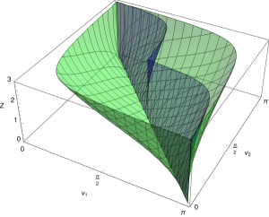
Figure 3: A plot of the possible effective states in the 3-dimensional parameter space of two nonspinning point particles that collide head-on, such that the solution has a moment of time symmetry: the parameters are $0\leq\nu_{1},\nu_{2}<\pi$ and $Z\geq 0$, which is equal both to the relative rapidity at impact, and the distance when the particles are momentarily at rest. (The particle spins and the impact parameter $D$ are assumed to be zero.) The boat-shaped green surface is $Z=C(\nu_{1},\nu_{2})$. Below and to the left of this surface (small $\nu_{i}$, small $Z$) the effective state is a virtual effective particle. Below and to the right (large $\nu_{i}$, small $Z$) the effective state is real third particle, which closes space. Above the surface (large $Z$), the effective state is a black hole. Within this black-hole region, for data to the right of the blue surface (large $\nu_{i}$) the moment of time symmetry (when the two particles are at maximum separation) already contains an apparent horizon.

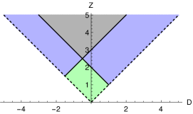
Figure 4: A plot of the different effective states for two massive spinning particles, plotted in the $(D,Z)$-plane, for arbitrarily fixed values $C_{+}=3$ and $C_{-}=2$. The plot continues to larger $Z$ and $|D|$. By definition $Z\geq|D|$, for $D$ to be interpreted as the (signed) impact parameter and $Z$ the relativity rapidity of the two particles at the moment of closest approach, or $|Z|$ as the apogee and $D$ as the perigee. In the green region, for $0\leq\nu_{1}+\nu_{2}<\pi$ spacetime at infinity is that of an effective spinning particle and the binary is eternal, while for $\nu_{1}+\nu_{2}>\pi$ space is closed by a real third particle and collapses. Blue corresponds to an overspinning particle, and grey to a spinning black hole. The regions and diagonal lines in the $(D,Z)$ plane here correspond to the regions and lines of the same colour in Fig. 2.

We now show that a point-particle effective state means an effective particle, and so a binary system orbiting forever, if and only if $\nu_{1}+\nu_{2}<\pi$, and a real third particle and closed space if and only if $\nu_{1}+\nu_{2}>\pi$, independently of the orbital parameters and particle spins.

To see this, consider first the limit where $Z$ and $D$ are much smaller than one. The two-particle orbit is then much smaller than the cosmological length scale $\ell$ and so spacetime outside the particles can be approximated as locally flat, and the particles are moving slowly, so special-relativistic effects can also be neglected. In this limit, the generator traces (144) are approximately

$$\left.\begin{aligned} Tu_{1}u_{2}\\ Tv_{1}v_{2}\end{aligned}\right\} \simeq \cos(\nu_{\mp 1}+\nu_{\mp 2})$$ (148)

$$= \cos\left(\nu_{1}+\nu_{2}\mp{\Delta{\hat{t}}_{1}+\Delta{\hat{t}}_{2}\over 2}\right)$$

$$=: \cos\left(\nu_{\text{tot}}\mp{\Delta{\hat{t}}_{\text{tot}}\over 2}\right).$$

Because of the periodicity of the cosine, this has multiple inverses for $\nu_{\text{tot}}$ and $(\Delta\hat{t})_{\text{tot}}$, and we now need to consider which choice of inverse is physical.

If $0\leq\nu_{1}+\nu_{2}\leq\pi$, the total defect angle is less than $2\pi$, and the excision wedges of the two particles (which in the $\Lambda=0$ approximation are straight lines) can be rotated so that they do not overlap. (Where one locates the wedges is otherwise pure gauge.) One then has a picture of time slices similar to that of Fig. 5 (in Appendix E): space is open, and outside both particles the spatial geometry is that of a cone, while seen from infinity the spatial slice is also a cone with vertex at a fictitious effective particle. From elementary Euclidean geometry, the defect angles add up to the total defect angles. Similarly, the time jumps add up when we go around both particle world lines. Hence the correct solution of (148) is

$$\nu_{\text{tot}}\simeq\nu_{1}+\nu_{2},\qquad\Delta\hat{t}_{\text{tot}}\simeq\Delta\hat{t}_{1}+\Delta\hat{t}_{2}.$$ (149)

(We have written $\simeq$ as a reminder that this is only an approximation for small, slow orbits.)

For $\nu_{1}+\nu_{2}>\pi$, the excision wedges have to overlap. Only a four-sided compact region of each time slice is now physical. If the particles are at A and B, and their excision wedges intersect at C and C’, for consistency we now must rotate the wedges so that C is mapped to C’ by the identification associated with either particle, in other words AC has the same length as AC’, and BC has the same length as BC’. The wedges now face each other symmetrically, and the triangles ABC and ABC’ are equal up to a reflection.

The vertices C and C’ now both represent a third particle that closes space: AC is glued to AC’, and BC to BC’, so that C and C’ coincide. Thus glued together, all three particles are on an equal footing. However, in the opened-up form, the entire physical angle around particle A is the angle CAC’, and similarly the entire physical angle around particle B is the angle CBC’, but the physical angle around particle C is split equally into the two sectors ACB and AC’B.

It is easy to see that for small orbits, where the curvature of spacetime can be neglected, the sum of physical angles around particles A, B and C is $2\pi$, namely the sum of interior angles of the two triangles ABC and ABC’. This means that the sum of the defect angles at the three particles is $3\times 2\pi-2\pi=4\pi$. This is the solid angle of $S^{2}$: each time slice has topology $S^{2}$, but the entire solid angle is concentrated at the three particles, with space flat in between. Beyond the small-orbit approximation, the curvature of space due to the cosmological constant also becomes significant. As this is negative for $\Lambda<0$, the sum of defect angles must be larger than $4\pi$.

With space closed, the total time jump going around all particles must be zero, as any loop going round all three particle world lines is contractible, that is, going around none. The correct solution of (148) for $\pi<\nu_{1}+\nu_{2}<2\pi$ is therefore

$$\nu_{1}+\nu_{2}+\nu_{3}\simeq 2\pi,\qquad\Delta\hat{t}_{1}+\Delta\hat{t}_{2}+\Delta\hat{t}_{3}\simeq 0.$$ (150)

Note that in this entire argument the wedge surfaces are independent of the particle spins, which only affect the time shift made in the identification, and so an effective particle is real if and only if $\nu_{1}+\nu_{2}>\pi$, independently of the particle spins. We now show that in the generic case, where $Z$ and $D$ are not small, this simple algebraic criterion still holds exactly.

As we have seen, the particle is real if the forward excision wedges overlap, and virtual if the backward excision wedges overlap. Suppose we start from a situation where the effective particle is real, and then reduce the defect angles of the two particles, while keeping their orbits and time jumps fixed. The real particle will move to the boundary of the adS3 cylinder, and return as a virtual particle. Hence the transition occurs when the effective particle is at infinity. This occurs when either $z$ or $\delta$ of the effective particle become infinite (an elliptic orbit reaching infinity), or both (a circular orbit at infinity). Hence, one or both of $\cosh z_{\pm}$ of the effective particle become infinite at the transition from real to effective particle.

Note now that when the matrices $u_{i}$ and $v_{i}$ are bounded, then so are $u_{1}u_{2}$ and $v_{1}v_{2}$. From (IV.5) we can write

$$\left.\begin{aligned} u_{1}u_{2}\\ v_{1}v_{2}\end{aligned}\right\}=\cos\nu_{{\rm tot}\mp}\,I+\sin\nu_{{\rm tot}\mp}\left(\cosh z_{{\rm tot}\mp}\,\gamma_{0}+\dots\right),$$ (151)

and this must remain bounded as the effective particle reaches infinity. Given that the coefficients of $\gamma_{0}$ in (151) must remain finite but one or both of $\cosh z_{{\rm tot}\mp}$ become infinite, we must have that the corresponding $\sin\nu_{{\rm tot}\mp}=0$ and so the corresponding $\cos\nu_{{\rm tot}\mp}=1$ or $-1$. In other words, an effective particle can be on an orbit reaching infinity only if either one of $Tu_{1}u_{2}$ or $Tv_{1}v_{2}$ is equal to either $1$ or $-1$, or both are.

Looking at the product traces now as the functions (144) of the initial parameters we see that, for fixed $\nu_{i\pm}$, $T=\pm 1$ occurs at the boundaries of the point-particle region in the $(D,Z)$ plane, so the effective particle cannot change nature within that region. But then we can choose to evaluate its nature in the small, slow orbit approximation $|D|,Z\ll 1$ as above. In other words, the effective particle is virtual for $\nu_{1}+\nu_{2}<\pi$ and real for $\nu_{1}+\nu_{2}>\pi$, independently of the $\Delta\hat{t}_{i}$, $D$ and $Z$.

VI.3 Two massless spinning particles

We now consider the case of two massless spinning particles. The special case of two non-spinning massless particles was treated in HM99 . The traces of the product generators are

$$\left.\begin{aligned} Tu_{1}u_{2}\\ Tv_{1}v_{2}\end{aligned}\right\} = 1-2e^{\mp D}(W_{1}\mp U_{1})(W_{2}\mp U_{2}).$$ (152)

In the massless limit, the rest frame and centre of mass conditions (141) become

$$e^{\pm\delta_{1}}(W_{1}\pm U_{1})=(1\leftrightarrow 2).$$ (153)

These two equations can be rearranged as

$$e^{\delta_{1}-\delta_{2}}={W_{2}+U_{2}\over W_{1}+U_{1}}={W_{1}-U_{1}\over W_{2}-U_{2}}.$$ (154)

and so $W_{1}$, $W_{2}$, $U_{1}$ and $U_{2}$ measured in the rest frame must obey the one constraint

$$W_{1}^{2}-U_{1}^{2}=W_{2}^{2}-U_{2}^{2}.$$ (155)

As we have $W_{i}>|U_{i}|$, we can parameterise this constraint as

$$W_{i}=W_{0}\cosh\sigma_{i},\quad U_{i}=W_{0}\sinh\sigma_{i}$$ (156)

where $W_{0}>0$ and $-\infty<\sigma_{i}<\infty$ can now be chosen freely. The two constraints (153) then both reduce to

$$\delta_{1}+\sigma_{1}=\delta_{2}+\sigma_{2}.$$ (157)

Given the gauge-invariant parameters $D$, $\sigma_{1}$ and $\sigma_{2}$, this can be solved for

$$\left.\begin{aligned} \delta_{1}\\ \delta_{2}\end{aligned}\right\}={D\pm(\sigma_{2}-\sigma_{1})\over 2}.$$ (158)

We then find

$$\left.\begin{aligned} Tu_{1}u_{2}\\ Tv_{1}v_{2}\end{aligned}\right\}=1-2W_{0}^{2}e^{\mp(D+\Sigma)},$$ (159)

where

$$\Sigma:=\sigma_{1}+\sigma_{2},$$ (160)

and the four gauge-invariant parameters $W_{0}$, $\sigma_{1}$, $\sigma_{2}$ and $D$ can be chosen freely. Substituting (158) into (143) gives

$$M\pm J={\cal Q}\left(1-2W_{0}^{2}e^{\pm(D+\Sigma)}\right),$$ (161)

and so $J$ is an odd analytic function of $D+\Sigma$ while $M$ is even.

The inequalities for classifying the effective state are

$$M_{\text{tot}}-J_{\text{tot}}>0 \quad\Leftrightarrow\quad D+\Sigma<2\ln W_{0},$$ (162a)

$$M_{\text{tot}}+J_{\text{tot}}>0 \quad\Leftrightarrow\quad D+\Sigma>-2\ln W_{0}.$$ (162b)

We see that it is a black hole state if and only if

$$|D+\Sigma|<2\ln W_{0},$$ (163)

which obviously requires $W_{0}>1$, a point particle if and only

$$|D+\Sigma|<-2\ln W_{0},$$ (164)

which requires $W_{0}<1$, and otherwise an overspinning particle state. We have the intuitive result that it is, qualitativey, the sum of orbital angular momentum and particle spins that impedes collapse. The non-spinning case is recovered simply by setting $\Sigma=0$, and for this case HM99 have shown that the black hole effective state corresponds to dynamical black hole formation, while for both the point particle and overspinning particle effective state the two particles leave through the conformal boundary. We conjecture that this holds also in the spinning case.

In the special case where two counterspinning particles of the same energy collide headon and merge into a single non-spinning massive point particle, or nonspinning black hole, we have $D=\Sigma=0$, and $\nu$ or $M$ are related to $W_{0}$ by $1-2W_{0}^{2}=\cos\nu$ for $W_{0}<1$ or $2W_{0}^{2}-1=\cosh\sqrt{M}$ for $W_{0}\geq 1$.

VI.4 One massive and one massless spinning particle

In the mixed case where particle 1 is massive and particle 2 is massless, and reparameterising

$$W_{2}=:W_{02}\cosh\sigma_{2},\quad U_{2}=:W_{02}\sinh\sigma_{2},$$ (165)

the traces of the product generators are

$$\left.\begin{aligned} Tu_{1}u_{2}\\ Tv_{1}v_{2}\end{aligned}\right\}=\cos\nu_{\mp 1}-\sin\nu_{\mp 1}\,W_{20}e^{z_{1}\mp(D+\sigma_{2})}.$$ (166)

The rest frame and centre of mass conditions (141) become

$$\sin(z_{1}\pm\delta_{1})\tan\nu_{\pm 1}=W_{20}e^{\mp(\delta_{2}+\sigma_{2})}.$$ (167)

Writing $\delta_{2}=D-\delta_{1}$ and eliminating $\delta_{1}$, we obtain

$$K^{2}+2K\cosh\tilde{D}+1=e^{4z_{1}}$$ (168)

where we have defined the shorthands

$$K := {2e^{z_{1}}W_{20}\over\sqrt{\tan\nu_{+1}\,\tan\nu_{-1}}},$$ (169a)

$$\alpha_{1} := {1\over 2}\ln{\tan\nu_{-1}\over\tan\nu_{+1}},$$ (169b)

$$\tilde{D} := D+\sigma_{2}+\alpha_{1}.$$ (169c)

$\tilde{D}$ is an impact parameter corrected for the spin of the massive particle (through $\alpha_{1}$) and the massless particle (through $\sigma_{2}$). We solve (168) as a quadratic equation for $K$, obtaining

$$K=-\cosh\tilde{D}+\sqrt{e^{4z_{1}}+\sinh^{2}\tilde{D}}.$$ (170)

Hence the product generator traces in their final form are

$$\left.\begin{aligned} Tu_{1}u_{2}\\ Tv_{1}v_{2}\end{aligned}\right\}=\cos\nu_{\mp 1}-{\sin\nu_{\mp 1}\,\tan\nu_{\mp 1}\over 2}e^{\mp\tilde{D}}K,$$ (171)

where the five gauge-invariant parameters $\nu_{\pm 1}$, $z_{1}$, $D$ and $\sigma_{2}$ can now be specified freely, and $K$ is given by (170). In the nonspinning case $J_{1}=U_{2}=0$ we have $\alpha_{1}=\sigma_{2}=0$ and $\tilde{D}=D$.

The inequalities for classifying the product isometry are

$$M_{\text{tot}}-J_{\text{tot}}>0 \quad\Leftrightarrow\quad \tilde{D}>\tilde{C}_{-},$$ (172a)

$$M_{\text{tot}}+J_{\text{tot}}>0 \quad\Leftrightarrow\quad \tilde{D}<\tilde{C}_{+},$$ (172b)

where we have defined the shorthands

$$\tilde{C}_{\pm} := \pm{1\over 2}\ln{e^{4z_{1}}-1-\hat{C}_{\mp}\over\hat{C}_{\mp}(\hat{C}_{\mp}+1)},$$ (173)

$$\hat{C}_{\pm} := 2\,{1+\cos\nu_{\pm 1}\over\sin\nu_{\pm 1}\,\tan\nu_{\mp 1}}.$$ (174)

In particular, we the effective state is a black hole for

$$\tilde{C}_{-}<\tilde{D}<\tilde{C}_{+}$$ (175)

(which implies $\tilde{C}_{-}<\tilde{C}_{+}$), an effective point particle for

$$\tilde{C}_{-}>\tilde{D}>\tilde{C}_{+}$$ (176)

(which implies $\tilde{C}_{-}>\tilde{C}_{+}$), and an effective overspinning particle otherwise. We conjecture that a black hole forms dynamically if and only if the effective state is a black hole, and otherwise the massless particle leaves the spacetime through the conformal boundary.

VII Conclusions

We have taken the first steps in a research programme of classifying all solutions of 2+1-dimensional general relativity with negative cosmological constant that contain two compact objects surrounded by vacuum.

The programme has three key ingredients: First, the exterior of any compact object must be an identification of adS3 under an isometry. Second, the same must be true for the exterior of the composite object. Third, we can obtain the composite isometry as a product of the component isometries representing two objects and their relative motion, as was first done in the $\Lambda=0$ case by Deser, Jackiw and t’Hooft DeserJackiwTHooft84 .

The possible exterior solutions for massive compact objects are precisely the BTZ axistationary vacuum solutions BTZ92 , which are parameterised by any real values of mass $M$ and spin $J$. These can be black holes $M\geq|J|$, point particles $M<-|J|$ and overspinning particles $|J|>|M|$. The black-hole solutions are very well studied, the particle solutions less so. In assembling our building blocks, we have filled a few small gaps in the literature, such as the maximal analytic extensions of the particle solutions and the nature of their singularities, and the construction of the overspinning particle solutions as identifications of adS3.

We can also admit the point particle and overspinning particle solutions on the entire domain $0<r<\infty$ as particle-like solutions. $r=0$ is a singular worldline only for non-spinning point particles, but otherwise is the boundary of a region of closed timelike curves that must be excised. (The singular worldline $\chi=0$ is inside this region.)

Finally, we can boost point particles while reducing their rest mass in order to create perfectly sensible massless (spinning particles) HM99 , and so these should be considered as well. (This probably makes no sense for extended objects with point particle exterior). This completes our list candidates for the two objects.

We have encountered two major difficulties in this programme. The first one is that while all real values of $(J,M)$ correspond to distinct BTZ solutions, the algebraic representation of the isometries of adS3 as the group $SL(2,{\mathbb{R}})\times SL(2,{\mathbb{R}})\times/{\mathbb{Z}}$ BHTZ93 covers only the segment $M>-1+|J|$ of the $(J,M)$ plane, comprising all black hole solutions but not all point particle or overspinning particle solutions.

The solutions we miss either have a time shift in their identification that is larger than $2\pi$, and/or an excess, rather than deficit, angle. There seems to be no reason for excluding these, and it is possible that the wider isometry group that generates them can be represented in a useful way. On the other hand, the space of rigidly rotating perfect fluid stars with causal barotropic equations of state constructed in 2+1rotstars fill precisely the region $M>-1+|J|$ of the $(J,M)$ plane, so it seems also possible that the exteriors of physically reasonable compact objects all fall into this region, which can be represented by the isometry group of padS3.

We can set aside this first difficulty by restricting ourselves to objects with $M_{i}>-1+|J_{i}|$ for $i=1,2$. Within this category, we have further restricted the two bodies to be to massive point particles or compact objects with massive point particle exterior, which have $-1+|J_{i}|<M_{i}<-|J_{i}|$ (the dark green region in Fig. 2), or massless point particles, which have $M_{i}=-1$, $J_{i}=0$ (but non-trivial isometry generators). We have computed $M_{\text{tot}}$ and $J_{\text{tot}}$ of the composite object as explicit analytic functions of six gauge-invariant parameters: the two rest masses and spins, and the impact parameter and energy in the center of mass frame.

The second major difficulty is how to draw conclusions about the global spacetime from the algebraic calculation. We have not attempted this, but rely on Holst and Matschull’s beautiful explicit construction of the global spacetime with two massless nonspinning point particles HM99 . Based on their work, we conjecture the following: if the product isometry corresponds to a black hole, a black hole is actually created dynamically. When the composite state of two massive particles is an overspinning particle, the binary is eternal. When it corresponds to a massive point particle, the binary is either eternal, or the effective particle is real and closes space, which then recollapses. We have found a simple criterion for which of the last two possibilities is realised. Finally, when either one or both of the two bodies is a massless particle and no black hole is formed the massless particle(s) leave the spacetime through the conformal boundary.

Our expressions for $M_{\text{tot}}$ and $J_{\text{tot}}$ remain finite and analytic at the black hole threshold. In this sense, there is no Choptuik-style critical scaling Choptuik92 ; GundlachLRR . The same is true also for toy models in 2+1 dimensions, such as dust balls MannRoss93 ; VazKoehler08 , thin dust shells PelegSteif95 , or shells with tangential pressure MannOh06 and rotation MannOhPark09 . All these systems cannot shed mass or spin so if a black hole is formed it contains all the mass and spin, and so the threshold of black hole formation is $|J_{\text{tot}}|=M_{\text{tot}}$. (By contrast, for 3+1 spacetime dimensions Kehle and Unger KehleUnger24 have made the exciting conjecture that there are regions of solution space where the threshold solutions are extremal black holes also for more physical matter models or even vacuum.)

However, a system that can shed mass and spin during collapse will show genuinely non-trivial critical phenoma even in 2+1 spacetime dimensions. This has been demonstrated for an axisymmetric massless scalar field without and with angular momentum in JalmuznaGundlachChmaj2015 ; JalmuznaGundlach2017 , and for an axisymmetric perfect fluid without and with angular momentum in BourgGundlach21a ; BourgGundlach21b .

What remains to be done to complete the solution of the two-body problem is to investigate the spacetimes where the two bodies include overspinning particles and black holes, or compact objects with such exteriors. We have not attempted this as we are not sure about the geometric meaning of the traces of the generator products. However, given that there are no periodic test particle orbits on black hole spacetimes, it is unlikely that eternal black hole binaries exist. Rather, it is likely that an effective point particle or overspinning particle is real and closes space, as in the solutions found in Clement94 .

It would also be interesting to see if BTZ solutions with $M>-1+|J|$ can be realised as identifications under an isometry of a spacetime we have called uadS3, with these isometries parameterised in form that allows them to be composed explicitly.

Appendix A $SO(2,2)$ and $SL(2,{\mathbb{R}})\times SL(2,{\mathbb{R}})/{\mathbb{Z}}^{2}$

It is helpful to translate the pair of $SL(2,{\mathbb{R}})$ generators into a single $SO(2,2)$ generator to see how the isometry acts on the hyperboloid (3) embedded in ${\mathbb{R}}^{(2,2)}$. We define the matrix $R\in SO(2,2)$ equivalent to the pair $(u,v)\in SL(2,{\mathbb{R}})\times SL(2,{\mathbb{R}})/{\mathbb{Z}}_{1}$ by

$$(RX)\cdot\gamma:=u^{-1}(X\cdot\gamma)v,$$ (177)

for all $X\in{\mathbb{R}}^{(2,2)}$, where $X\cdot\gamma$ is shorthand for (62). Recall that we use the coordinates $X=(x_{3},x_{0},x_{1},x_{2})$, where we denote the two timelike directions by $(x_{3},x_{0})$. This definition gives the explicit formula

$$R_{\mu\nu}={1\over 2}(-1)^{\delta_{\mu 0}}\operatorname{tr}\left(\gamma_{\mu}u^{-1}\gamma_{\nu}v\right)$$ (178)

for the components of the matrix $R$. If we write $u=\sum u_{\mu}\gamma_{\mu}$, where $u_{0}^{2}+u_{3}^{2}-u_{1}^{2}-u_{2}^{2}=1$, and similarly for $v$, then each matrix element $R_{\mu\nu}$ of $R$ is a sum of four terms of the form $u_{\alpha}v_{\beta}$.

Consider now the $SO(2,2)$ matrix $S$ equivalent to the pair of $SL(2,{\mathbb{R}})$ matrices $(u,I)$, and $T$ equivalent to the pair $(I,v)$. The generators of the product of these isometries, in either order, are $(u,v)$ and so we must have $R=ST=TS$. Moreover, for a given isometry $u$ and $v$ are unique up to an overall sign. This implies any $SO(2,2)$ matrix $R$ can be written as the product of two commuting $SO(2,2)$ factors $S$ and $T$. However, the isometries $(u^{p},v^{q})$ and $(u^{1-p},v^{1-q})$, whose product is $(u,v)$, also commute, and so the split is not unique.

We define the 6 one-parameter subgroups $R_{[\mu\nu]}(\alpha)$ of $SO(2,2)$, with $\mu>\nu$, $\mu,\nu=3,0,1,2$, as the group of rotations or boosts in the $(x_{\mu},x_{\nu})$-plane. The subgroups $R_{\mu\nu}$ and $R_{\kappa\lambda}$ commute if and only if $\mu,\nu,\kappa,\lambda$ are all distinct, and so the 6 one-parameter subgroups form three pairs of one-parameter commuting subgroups. We can trivially combine these pairs into the 3 two-parameter subgroups

$$R_{[30][12]}(\alpha,\beta) := R_{[30]}(\alpha)\,R_{[12]}(\beta),$$ (179)

$$R_{[31][02]}(\alpha,\beta) := R_{[31]}(\alpha)\,R_{[02]}(\beta),$$ (180)

$$R_{[32][01]}(\alpha,\beta) := R_{[32]}(\alpha)\,R_{[01]}(\beta).$$ (181)

Less obviously, we can restrict these two obtain six more pairs of two commuting one-parameter subgroups, namely

$$\left[R_{[30][12]}(\alpha,\alpha),R_{[31][02]}(\beta,\beta)\right] = 0,$$ (182)

$$\left[R_{[30][12]}(-\alpha,\alpha),R_{[31][02]}(-\beta,\beta)\right] = 0,$$ (183)

$$\left[R_{[30][12]}(-\alpha,\alpha),R_{[32][01]}(\beta,\beta)\right] = 0,$$ (184)

$$\left[R_{[30][12]}(\alpha,\alpha),R_{[32][01]}(-\beta,\beta)\right] = 0,$$ (185)

$$\left[R_{[32][01]}(\alpha,\alpha),R_{[31][02]}(\beta,\beta)\right] = 0,$$ (186)

$$\left[R_{[32][01]}(-\alpha,\alpha),R_{[31][02]}(-\beta,\beta)\right] = 0.$$ (187)

Appendix B $SO(2,2)$ derivation of the overspinning particle cut-and-paste coordinates

We now use the formulas of Appendix A to derive a parameterisation of (3) for the overspinning case $|J|>|M|$. In the context of this paper we need it to prove that (81,82) really are the generators for $J>|M|$ and $J<|M|$, respectively.

The $SO(2,2)$ equivalent of the black hole generators (77) is

$$R_{\rm bh}:=R_{[32][01]}(2\pi s_{-},-2\pi s_{+}).$$ (188)

The two commuting factors corresponding to $(u,I)$ and $(I,v)$ are

$$T_{\rm bh} := R_{[32][01]}(-\pi\lambda_{+-},-\pi\lambda_{+-}),$$ (189)

$$S_{\rm bh} := R_{[32][01]}(\pi\lambda_{++},-\pi\lambda_{++}).$$ (190)

The three parameterisations $X({\hat{t}},\chi,{\hat{\phi}})$ of (3) for black holes can be written as

$$X_{\rm outer} = R_{[32][01]}({-\hat{t},-\hat{\phi}})\,R_{[02]}(-\chi)\,(0,-1,0,0),$$

$$X_{\rm middle} = R_{[32][01]}({-\hat{t},-\hat{\phi}})\,R_{[30]}(-\chi)\,(-1,0,0,0),$$

$$X_{\rm inner} = R_{[32][01]}({-\hat{t},-\hat{\phi}})\,,R_{[31]}(-\chi)\,(-1,0,0,0).$$

This notation makes it easy to verify that all three parameterisations $X$ obey

$$R_{\rm bh}X({\hat{t}},\chi,{\hat{\phi}})=X({\hat{t}}-2\pi s_{-},\chi,{\hat{\phi}}+2\pi s_{+}),$$ (192)

using that $R_{32}$ and $R_{01}$ commute, and the defining property of 1-parameter subgroups that $R(\alpha)R(\beta)=R(\alpha+\beta)$.

Similarly, the equivalent of the point particle generators (79) is

$$R_{\rm pp}:=R_{[30][12]}(-2\pi a_{-},-2\pi a_{+}),$$ (193)

with commuting factors

$$T_{\rm pp} := R_{[30][12]}(-\pi\lambda_{-+},-\pi\lambda_{-+}),$$ (194)

$$S_{\rm pp} := R_{[30][12]}(\pi\lambda_{--},-\pi\lambda_{--}),$$ (195)

and the parameterisation is

$$X_{\rm pp}=R_{[30][12]}(-{\hat{t}},-{\hat{\phi}})\,R_{31}(\chi)\,(1,0,0,0),$$ (196)

and the pair obeys

$$R_{\rm pp}X_{\rm pp}({\hat{t}},\chi,{\hat{\phi}})=X({\hat{t}}+2\pi a_{-},\chi,{\hat{\phi}}+2\pi a_{+}).$$ (197)

Based on these examples, we now see what to do in the overspinning particle case. We only deal with the case $J>|M|$, as the case $J<-|M|$ is similar. The $SO(2,2)$ generator is

$$R_{J>|M|}:=T_{\text{pp}}S_{\text{bh}}.$$ (198)

The crucial observation is that the $T_{\text{pp}}$ and $S_{\text{bh}}$ still commute because of (185). This allows us to write

$$X_{J>|M|} = R_{[32][01]}(\hat{\phi},-\hat{\phi})R_{[30][12]}(-\hat{t},-\hat{t})$$ (199)

$$\times R_{02}(\chi)\,(0,1,0,0),$$

and to verify that $R_{J>|M|}X_{J>|M|}\sim X_{J>|M|}$ is equivalent to (52). The parameterisation (199) is written out in full in the last column of Table 1. Instead of the last factor in (199) we could have used $R_{31}(-\chi)\,(1,0,0,0)$ to obtain the same induced metric.

Appendix C The limit $\Lambda=0$

To take the limit $\Lambda\to 0$, or equivalently $\ell\to\infty$, we use dimensional analysis to reinstate $\ell$ in the relevant formulas, using that $J$ and our radial and time coordinates have dimension length, while $M$ and angles are dimensionless.

The metric of a spinning point particle solution of (1) with $\Lambda=0$, with mass $m$ and spin (angular momentum) $j$ at rest at the origin of the coordinate system can be written as the flat metric

$$ds^{2}=-d{\hat{t}}^{2}+d\chi^{2}+\chi^{2}\,d{\hat{\phi}}^{2}$$ (200)

but with the non-trivial identifications

$$({\hat{t}},\chi,{\hat{\phi}})\sim\left({\hat{t}}+\Delta\hat{t}_{\rm pp},\chi,{\hat{\phi}}+(2\pi-2\nu)\right),$$ (201)

where the defect angle $2\nu$ and time jump $\Delta\hat{t}_{\rm p}$ are given by

$$\nu = 4\pi m,$$ (202)

$$\Delta\hat{t}_{\rm pp} = (1-4m)8\pi j,$$ (203)

in units $c=G=1$, compare Eqs. (2.8b-c) and (4.21-22) of DeserJackiwTHooft84 and Eq. (1) of DeserJackiwTHooft92 . Here $m$ and $j$ are defined as area integrals over a distributional stress-energy tensor $T_{ab}$ in Eq. (1), following DeserJackiwTHooft84 . In the limit $\ell\to\infty$, $\nu$ defined in (47) and $\nu_{\pm}$ defined in (80) all become become equal to $\nu$ defined in (202).

On small spacetime scales the cosmological constant becomes irrelevant, and so has no influence on the conical singularity itself. Indeed, in the limit $\ell\to\infty$, the point particle metric (7) in cut-and-paste coordinates becomes (200).

Using $a_{+}\to\sqrt{-M}$ and $a_{-}\ell\to J/(2\sqrt{-M})$ (and hence $a_{-}\to 0$ and $a_{-}/\ell\to 0$) as $\ell\to\infty$ we find that in this limit the definitions (42) become

$${\chi} = {1\over\sqrt{-M}}\sqrt{r^{2}+{J^{2}\over 4(-M)}},$$ (204)

$$\ {\hat{t}} = \sqrt{-M}t+{J\over 2\sqrt{-M}}\phi,$$ (205)

$${\hat{\phi}} = \sqrt{-M}\phi.$$ (206)

The resulting metric is again the BTZ metric (23), with the only difference that now

$$f=-M+{J^{2}\over 4r^{2}}.$$ (207)

This is agrees with taking the limit $\ell\to\infty$ directly in (23,24) while keeping $M$ and $J$ fixed.

We note that $f=0$ corresponds to $\chi=0$, whereas $r=0$ corresponds to $\chi=|J|/(-2M)$. From the argument given above in Sec. II.5, we see that by restricting to $r>0$ we eliminate CTCs.

This important fact is not explicitly noted in DeserJackiwTHooft84 , perhaps because the significance of $\chi=|J|/(-2M)$ is less obvious in the cut-and-paste metric (200) than that of $r=0$ in the BTZ-like metric (23) with (207). Conversely, in MiskovicZanelli2009 the point-particle BTZ metric is interpreted as having a brane source at $r=0$, rather than a point particle at $\chi=0$, and the possible extension beyond $r=0$ is not explicitly noted.

The identification $(t,r,\phi)\sim(t,r,\phi+2\pi)$ corresponds

$$({\hat{t}},\chi,{\hat{\phi}})\sim\left({\hat{t}}+{J\over 2\sqrt{-M}}2\pi,\chi,{\hat{\phi}}+\sqrt{-M}2\pi\right),$$ (208)

and so in the limit $\Lambda\to 0$ the point particle defect angle and time jump are related to the BTZ quantities as

$$\nu = \pi\left(1-\sqrt{-M}\right),$$ (209)

$$\Delta\hat{t}_{\rm pp} = {\pi J\over\sqrt{-M}}.$$ (210)

These expressions are equal to the leading orders in $\Lambda=-\ell^{-2}$ in the corresponding expressions (47) and (48). However, in interpreting them one should keep in mind that $\nu$ and $\Delta\hat{t}_{\rm pp}$ can be measured in an arbitrarily small neighbourhood of the particle world line, and so should be interpreted as fundamental properties of the particle, independently of $\Lambda$, while $M$ and $J$ should be considered as depending on both the particle and $\Lambda$.

As a byproduct of our calculations for $\Lambda<0$, we can also obtain the expressions for the total mass and angular momentum of the effective final particle in the case $\Lambda=0$, when black holes cannot form. For this purpose, we simply note that the only dimensionful parameter of the initial data is $D$, which has units of length and so is measured in units of $\ell$. Among the parameters of the final state, the same holds for the time jump $\Delta\hat{t}$. Equating (144) with (79), taking the sum and difference of the equations with the two signs, and expanding to leading order in $1/\ell$, we find

$$\cos\nu_{\text{tot}} = \cos\nu_{1}\cos\nu_{2}-\sin\nu_{1}\sin\nu_{2}\cosh Z,$$

$$\Delta\hat{t}_{\text{tot}}\sin\nu_{\text{tot}} = \Delta\hat{t}_{1}(\sin\nu_{1}\cos\nu_{2}+\cos\nu_{1}\sin\nu_{2}\cosh Z)$$

$$+(1\leftrightarrow 2)+2D\sin\nu_{1}\sin\nu_{2}\sinh Z.$$

Note that the first equation is valid also for spinning point particles, even though the time jumps representing the spin do not appear.

Eq. (C) is the the same as Eq. (5.12) of DeserJackiwTHooft84 , whereas the angular momentum $j$ of the effective point particle was computed there only in a Newtonian approximation. To check agreement with that result, we expand in $\nu_{i}\ll 1$ and $Z\ll 1$. Noting that $Z\simeq{v_{1}+v_{2}}$ for small $Z$, we find

$$\nu \simeq \nu_{1}+\nu_{2},$$ (213)

$$\Delta\hat{t}_{\rm pp} \simeq 2{\nu_{1}\nu_{2}\over\nu_{1}+\nu_{2}}D\,(v_{1}+v_{2}).$$ (214)

For $\nu_{1}=\nu_{2}$ and hence $v_{1}=v_{2}$, this last equation reduces to $\Delta\hat{t}_{\rm pp}\simeq 2\nu_{1}Dv_{1}$, which agrees with Eq. (5.20) of DeserJackiwTHooft84 if we also approximate the right-hand side of (203) by $8j$. (Note that in units $c=G=1$, $J$ of DeserJackiwTHooft84 is our $j$.)

We note that the authors of DeserJackiwTHooft84 impose as the rest frame condition that the effective particle is at rest in one of the two product orders (but therefore not the other), whereas our rest frame condition is that the effective particle moves with equal and opposite velocities in the two product orders. We believe our condition, which is based on the clear physical argument set out in Sec. V.2, is better motivated.

Appendix D A geometric construction of an effective particle with $\Lambda=0$

Fig. 5 illustrates a time slice with $\Lambda=0$ and two point particles with masses (half of defect angles) $\nu_{1}$ and $\nu_{2}$ at rest at positions $(0,0)$ and $(0,d)$. The following statements can be verified by inspection of this figure:

(1) A time slice is obtained by gluing together the entire shaded region (that is, counting the overlap only once) together along the two wedges. The resulting geometry, when embedded like a piece of paper into 3-dimensional Euclidean space, looks like a coffee filter paper. Let us call this manifold 1.

(2) By contrast, the effective geometry seen from a distance is obtained by moving the upper (blue) and lower (red) shaded patches apart until their vertices (represented by the two larger dots, with the corresponding colors) coincide before gluing them together. The total defect angle at the new vertex (where the two larger dots are now identified) is $2\nu_{1}+2\nu_{2}$. Note that the doubly-shaded region of space has to be duplicated for this construction. Let us call the result manifold 2.

(3) The new vertex has a unique position on manifold 2 (which is larger), but not on manifold 1. If on each of the two patches on manifold 1 we keep the Cartesian coordinate system $(x,y)$ defined by the horizontal and vertical axes before the patches are moved then the location of the effective particle is

$$(x_{0},y_{0}):=d{\sin\nu_{2}\over\sin(\nu_{1}+\nu_{2})}(\cos\nu_{1},\sin\nu_{1})$$ (215)

when seen from the lower (red) patch, but $(x_{0},-y_{0})$ when seen from the upper (blue) patch.

(4) Seen from the upper (blue) patch, going anticlockwise around the effective particle is equivalent to going anticlockwise around particle 1 then particle 2. Seen from the lower (red) patch, this order is reversed. Hence the two product orders correspond to different coordinate choices on the two-particle spacetime.

By making $d$ slowly time-dependent, we can also infer the geometry of two moving particles in the limit of non-relativistic motion: If the particles approach each other horizontally at a combined speed $2v$, then the two fictitious locations of the effective particle approach each other vertically, each at speed of $v_{\text{tot}}=2v\sin\nu_{1}\nu_{2}/\sin(\nu_{1}+\nu_{2})$. For $\nu_{1}=\nu_{2}=\nu$ and $v_{1}=v_{2}=v$, we have $v_{\text{tot}}=v\tan\nu$. This agrees with the non-relativistic limit $|v|\ll 1$ of (128b), and $\nu_{\text{tot}}=\nu_{1}+\nu_{2}$ agrees with (128a). (At higher velocity, special-relativistic velocity addition and mass increase would have to be taken into account).

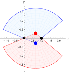
Figure 5: Construction of the spatial geometry with $\Lambda=0$ and two point particles with masses (half of defect angles) $\nu_{1}$ and $\nu_{2}$ at positions $(0,0)$ and $(0,d)$, represented by the two smaller (black) dots. The area of each dot is proportional to the mass (defect angle) of the particle it represents. For plotting we have chosen the specific values $\nu_{1}=0.4$, $\nu_{2}=0.7$, and $d=1.0$.

Appendix E The head-on collision of two non-spinning massive particles

Steif Steif96 has classified all time-symmetric initial data for the two-body problem. The two bodies can then be nonspinning black holes or nonspinning massive point particles.

For the case of two point particles, we have the 3-dimensional subcase of our 6-dimensional space of initial data where two non-spinning massive particles collide head-on. This requires that the particle spins and the impact parameter $D$ all vanish. In our units where $\Lambda=-1$ and $G=c=1$, our parameter $M$ is $8M$ of Steif, our $\nu_{1}$ and $\nu_{2}$ are $4\pi m$ and $4\pi\tilde{m}$ of Steif, and our $Z$ is $d$ of Steif. Recall that $Z$ is both the rapidity at closest approach (here, at impact), and the distance at largest separation (here, at the moment of time symmetry). Rather than the full spacetime, Steif constructs the initial data at the moment of time symmetry, where the extrinsic curvature vanishes. The spatial geometry at that moment is constructed by isometric identifications of the Poincaré disk, corresponding to our identifications of the entire spacetime. Note that for easier comparison with Steif’s work we have adapted a convention throughout this paper where $u=v$ if and only if the spacetime admits a moment of time symmetry, and this single element of $SL(2,{\mathbb{R}})$ then parameterises an isometry of ${\mathbb{H}}^{2}$.

Our results agree with Steif’s with the following clarifications: his “open, no horizon” can denote both our virtual effective particle outcome, or our black hole outcome. In the latter case, a black hole forms eventually as the particles fall toward each other from a large separation, but there is no apparent horizon at the moment of time symmetry (moment of largest separation). “Closed space” corresponds to our real effective particle outcome. In other words, this is really a three-particle closed universe that recollapses. “Black hole” corresponds to our black hole outcome and where an apparent horizon is already present at the moment of time symmetry. Our black hole criterion $Z>C$ corresponds to $\cosh d>f_{c}$ of Steif. Our and Steif’s results are shown in Fig. 3. For completeness, we have included in this figure, without derivation, Steif’s criterion for the existence of an AH at the moment of time symmetry. This is $d<\tan\nu_{1}/(-\tan\nu_{2})$ for $0\leq\nu_{1}\leq\pi/2$ and $\pi/2<\nu_{2}<\pi$, and equivalently for $\nu_{1}$ and $\nu_{2}$ interchanged. The derivation, not given in Steif96 , will be given elsewhere Jormatwoparticles .

When the two original particles are equivalent to an effective particle and collide head-on but a black hole does not form, one can take them to collide elastically, bouncing back from the collision event, or to collide inelastically, continuing as a single particle with mass $\nu_{\text{tot}}\pi$.

In the elastic collision, one basically wants to glue one spacetime picture, including the wedges, to its mirror image under a time reflection through $t=0$. This is possible only if the restrictions of the two sides of each wedge to $t=0$ are mapped to each other, and this in turn requires the wedges to be centred on the plane through the two particle trajectories, and facing away from each other.

For the inelastic collision, one could arrange one side of each excision wedge to touch at the moment of collision, and for the other two sides to become, at that moment, the two sides of the excision wedge of the new particle.

References

- (1) S. Deser, R. Jackiw and G. t’Hooft, Three-dimensional Einstein gravity: Dynamics of flat space, Annals of Physics 152, 220 (1984).
- (2) M. Bañados, C. Teitelboim and J. Zanelli, Black hole in three-dimensional spacetime, Phys. Rev. Lett. 69, 1849 (1992).
- (3) M. Bañados, M. Henneaux, C. Teitelboim and J. Zanelli, Geometry of the 2+1 black hole, Phys. Rev. D 48, 1506 (1993).
- (4) The large scale structure of spacetime, S. W. Hawking and G. F. R. Ellis, Cambridge University Press 1973.
- (5) A. R. Steif, Time-symmetric initial data for multibody solutions in three dimensions, Phys. Rev. D 53, 5527 (1996).
- (6) H.-J. Matschull, Black hole creation in 2 + 1 dimensions, Class. Quant. Grav. 16, 1069 (1999).
- (7) S. Holst and H.-J. Matschull, The anti-de Sitter Gott universe: a rotating BTZ wormhole, Class. Quant. Grav. 16, 3095 (1999).
- (8) J. Lindgren, Black hole formation from pointlike particles in three-dimensional anti-de Sitter space, Class. Quant. Grav. 33, 145009 (2016).
- (9) J. Lindgren, Collisions of massive particles, timelike thin shells and formation of black holes in three dimensions, J. High Energy Phys. 2016, 48 (2016).
- (10) J. R. Gott III, Closed timelike curves produced by pairs of moving cosmic strings: Exact solutions, Phys. Rev. Lett. 66, 1126 (1991).
- (11) S. Carlip, The (2+1)-dimensional black hole, Class. Quant. Grav. 12, 2853 (1995).
- (12) O. Mišković and J. Zanelli, Negative spectrum of the 2+1 black hole, Phys. Rev. D 79, 105011 (2009).
- (13) D. Birmingham and S. Sen, Gott time machines, BTZ black hole formation, and Choptuik scaling, Phys. Rev. Lett. 84, 1074 (2000).
- (14) S. Deser, R. Jackiw and G. T’Hooft, Physical cosmic strings do not generate closed timelike curves, Phys. Rev. Lett. 68, 267 (1992).
- (15) I. Bengtsson and P. Sandin, Anti-de Sitter space, squashed and stretched, Class. Quant. Grav. 23, 971 (2006).
- (16) C. Gundlach and P. Bourg, Rigidly rotating perfect fluid stars in 2+1 dimensions, Phys. Rev. D 102, 084023 (2020).
- (17) M. Cataldo, Rotating perfect fluids in (2+1)-dimensional Einstein gravity, Phys. Rev. D 69, 064015 (2004).
- (18) M. W. Choptuik, Universality and scaling in gravitational collapse of a massless scalar field, Phys. Rev. Lett. 70, 9 (1993).
- (19) C. Gundlach and J. M. Martín-García, Living Rev. Relativity, 2007-05 (2007).
- (20) R. B. Mann and S. F. Ross, Gravitationally collapsing dust in 2+1 dimensions, Phys. Rev. D 47, 3319 (1993).
- (21) C. Vaz and K. R. Koehler, Rotating, inhomogeneous dust interior for the BTZ black hole, Phys. Rev. D 78, 024038 (2008).
- (22) Y. Peleg and A. R. Steif, Phase transition for gravitationally collapsing dust shells in 2+1 dimensions, Phys. Rev. D, 51, R3992 (1995).
- (23) R. B. Mann and J. J. Oh, Gravitationally collapsing shells in (2+1) dimensions, Phys. Rev. D 74, 124016 (2006).
- (24) R. B. Mann J. J. Oh and M. Park, Role of angular momentum and cosmic censorship in (2+1)-dimensional rotating shell collapse, Phys. Rev. D 79, 064005 (2009).
- (25) C. Kehle and R. Unger, Extremal black hole formation as a critical phenomenon, unpublished, https://arxiv.org/abs/2402.10190.
- (26) J. Jałmużna, C. Gundlach, and T. Chmaj, Scalar field critical collapse in 2+1 dimensions, Phys. Rev. D 92, 124044 (2015).
- (27) J. Jałmużna and C. Gundlach, Critical collapse of a rotating scalar field in 2+1 dimensions, Phys. Rev. D 95, 084001 (2017).
- (28) P. Bourg and C. Gundlach, Critical collapse of a spherically symmetric ultrarelativistic fluid in 2+1 dimensions, Phys. Rev. D 103, 124055 (2021).
- (29) P. Bourg and C. Gundlach, Critical collapse of an axisymmetric ultrarelativistic fluid in 2+1 dimensions, Phys. Rev. D 104, 104017 (2021).
- (30) G. Clément, Multiwormholes and multi-black-holes in three dimensions, Phys. Rev. D 50, R7119 (1994).
- (31) J. Louko, unpublished notes.