Small $x$ asymptotics for special function solutions of Painlevé III equation

Abstract.

In this paper we compute the small $x$ asymptotics of the special function solutions of Painlevé-III equation. We use the representation of solution in terms of Hankel determinants of Bessel functions, which seems to be new. Hankel determinants can be rewritten as multiple contour integrals using Andrèief identity. Finally small $x$ asymptotics is obtained using elementary asymptotic methods.

1. Introduction

Painlevé equations are six nonlinear second-order ordinary differential equations. They are written in the form of $u^{\prime\prime}=R(u^{\prime},u,t)$ with $R$ a rational function. Their solutions have the so called Painlevé property. It means that the locations of singularities of branching type don’t depend on the initial conditions, but the locations of isolated singularities might depend on initial conditions. They were discovered at the beginning of the 20st century in the works [Pai02, Gam10], see also [Inc44]. Most of the solutions of Painlevé equations are transcendental. It means that they can’t be reduced to simpler classical special functions. However, there are several exceptions. In particular for Painlevé III equation one can find solutions expressed in terms of Bessel functions (see [UW98, Mur95]). For the applications of such special function solutions of Painlevé III equation in random matrix theory we refer the reader to [FW02], [ZCL20].

We start with presenting Painlevé III equation

$$u^{\prime\prime}=\dfrac{\left(u^{\prime}\right)^{2}}{u}-\dfrac{u^{\prime}}{x}+\dfrac{\alpha u^{2}+\beta}{x}+u^{3}-\frac{1}{u},\quad\alpha,\beta\in\mathbb{C}.$$ (1)

Consider the Hankel determinant of cylinder functions:

$$\Delta_{n}(x,\alpha)=\det\left(\left\{\mathcal{C}_{\frac{\alpha}{2}-j+k}(x)\right\}_{j,k=0}^{n-1}\right),\quad n\in\mathbb{N}$$ (2)

with

$$\mathcal{C}_{\nu}(x)=d_{1}J_{\nu}(x)+d_{2}Y_{\nu}(x)$$ (3)

and $J_{\nu}(x)$, $Y_{\nu}(x)$ are Bessel functions of first and second kind. Additionally, denote $\Delta_{0}(x,\alpha)=1$.

Proposition 1.1.

The expression

$$u_{n}(x,\alpha)=-\frac{\Delta_{n+1}(x,\alpha-2)\Delta_{n}(x,\alpha)}{\Delta_{n+1}(x,\alpha)\Delta_{n}(x,\alpha-2)},\quad n\in\mathbb{N}\cup\{0\},\quad\alpha\in\mathbb{C}.$$ (4)

solves Painlevé III equation with shifted parameters

$$u_{n}^{\prime\prime}=\dfrac{\left(u_{n}^{\prime}\right)^{2}}{u_{n}}-\dfrac{u_{n}^{\prime}}{x}+\dfrac{(\alpha+2n)u_{n}^{2}+(-\alpha+2+2n)}{x}+u_{n}^{3}-\frac{1}{u_{n}}.$$ (5)

The fact that Hankel determinants of Bessel functions are related to the solutions of Painlevé III equation is well known, see for example [Cla23], [FW02]. But the formula of type (4) was not presented in literature, except for the case of rational solutions, see [CLL23]. Now we are ready to present the first result of our asymptotic analysis.

Theorem 1.1.

The Hankel determinant (2) admits the following $x\rightarrow 0$ asymptotics for fixed $d_{1},d_{2}\in\mathbb{C}$, $n\in\mathbb{N}\cup\{0\}$, $\alpha\in\mathbb{C}\setminus(2\mathbb{Z}+i\mathbb{R})$

1. If $Re(\alpha)>2n-2\text{ or }d_{1}\sin\left(\frac{\pi\alpha}{2}\right)+d_{2}\cos\left(\frac{\pi\alpha}{2}\right)=0$, then

   $$\Delta_{n}(x,\alpha)\sim(-1)^{\frac{n(n+1)}{2}}\left(\frac{d_{2}}{\pi}\right)^{n}\frac{G(n+1)G(\frac{\alpha}{2}+1)}{G(\frac{\alpha}{2}-n+1)}\left(\frac{x}{2}\right)^{-\frac{n\alpha}{2}},\text{ as }x\to 0.$$

2. If $2n-4j-2<Re(\alpha)<2n-4j+2\text{ for }j=1,2\ldots,n-1$, then

   $$\Delta_{n}(x,\alpha)\sim (-1)^{\frac{n(n-1)}{2}+nj+n-j}\left(\frac{d_{2}}{\pi}\right)^{n}\left(\frac{d_{1}}{d_{2}}\sin\left(\frac{\pi\alpha}{2}\right)+\cos\left(\frac{\pi\alpha}{2}\right)\right)^{j}$$

   $$\times\frac{G(n-j+1)G(-\frac{\alpha}{2}+n-j+1)G(j+1)G(j+\frac{\alpha}{2}+1)}{G(-\frac{\alpha}{2}+n-2j+1)G(\frac{\alpha}{2}-n+2j+1)}\left(\frac{x}{2}\right)^{(\alpha-2n+2j)j-\frac{n\alpha}{2}},\text{ as }x\to 0.$$

3. If $Re(\alpha)<-2n+2\text{ or }d_{2}=0$, then

   $$\Delta_{n}(x,\alpha)\sim\frac{(-1)^{\frac{n(n+1)}{2}}}{\pi^{n}}\left(d_{1}\sin\left(\frac{\pi\alpha}{2}\right)+d_{2}\cos\left(\frac{\pi\alpha}{2}\right)\right)^{n}\frac{G(n+1)G(-\frac{\alpha}{2}+1)}{G(-\frac{\alpha}{2}-n+1)}\left(\frac{x}{2}\right)^{\frac{n\alpha}{2}},\text{ as }x\to 0$$

where $G(x)$ refers to the Barnes $G$-function.

This formula is obtained after rewriting the Hankel determinant as multiple contour integral using Andrèief identity and performing elementary asymptotic analysis. We should mention that the same strategy was applied to special function solutions of Painlevé-II equation in [Dea18].

Combining the Theorem 1.1 with Proposition 1.1 we derive the asymptotics of $u_{n}(x,\alpha)$ as $x\rightarrow 0$.

Theorem 1.2.

Solution (4) of Painlevé-III equation (5) admits the following $x\rightarrow 0$ asymptotics for fixed $d_{1},d_{2}\in\mathbb{C}$, $n\in\mathbb{N}\cup\{0\}$, $\alpha\in\mathbb{C}\setminus(2\mathbb{Z}+i\mathbb{R})$

1. If $Re(\alpha)>2+2n\quad\text{or }d_{1}\sin\left(\frac{\pi\alpha}{2}\right)+d_{2}\cos\left(\frac{\pi\alpha}{2}\right)=0$, then

   $$u_{n}(x,\alpha)\sim\left(\frac{2}{2n+2-\alpha}\right)\frac{x}{2},\text{ as }x\to 0.$$

2. If $2n-4j<Re(\alpha)<2n-4j+2\text{ and }j=0,1,\ldots,n$,then

   $$u_{n}(x,\alpha)\sim (-1)^{n}\left(\frac{d_{1}}{d_{2}}\sin\left(\frac{\pi\alpha}{2}\right)+\cos\left(\frac{\pi\alpha}{2}\right)\right)\left(\frac{\Gamma(-\frac{\alpha}{2}+n-2j+1)}{\Gamma(\frac{\alpha}{2}-n+2j)}\right)^{2}$$

   $$\times\frac{\Gamma(j+\frac{\alpha}{2})\Gamma(j+1)}{\Gamma(-\frac{\alpha}{2}+n-j+1)\Gamma(n-j+1)}\left(\frac{x}{2}\right)^{\alpha-2n+4j-1},\text{ as }x\to 0.$$

3. If $2n-4j-2<Re(\alpha)<2n-4j\text{ and }j=0,1,\ldots,n-1$, then

   $$u_{n}(x,\alpha)\sim (-1)^{n}\left(\frac{d_{1}}{d_{2}}\sin\left(\frac{\pi\alpha}{2}\right)+\cos\left(\frac{\pi\alpha}{2}\right)\right)^{-1}\left(\frac{\Gamma(\frac{\alpha}{2}-n+2j+1)}{\Gamma(-\frac{\alpha}{2}+n-2j)}\right)^{2}$$

   $$\times\frac{\Gamma(-\frac{\alpha}{2}+n-j+1)\Gamma(n-j)}{\Gamma(j+\frac{\alpha}{2}+1)\Gamma(j+1)}\left(\frac{x}{2}\right)^{-\alpha+2n-4j-1},\text{ as }x\to 0.$$

4. If $Re(\alpha)<-2n\quad\text{or }d_{2}=0$, then

   $$u_{n}(x,\alpha)\sim\left(-\frac{\alpha}{2}-n\right)\left(\frac{x}{2}\right)^{-1},\text{ as }x\to 0.$$

where $\Gamma(x)$ refers to the Gamma function.

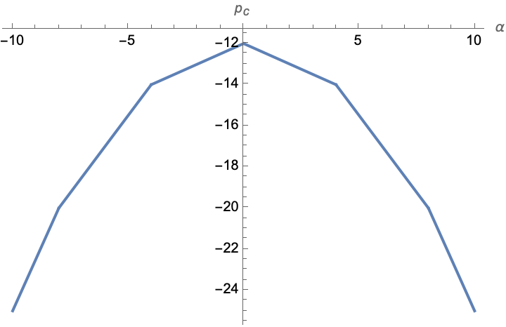
(a) Hankel determinant

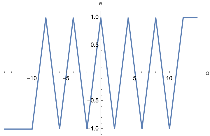
(b) Solution of Painlevé-III equation.

Figure 1. Leading power in the asymptotics for $n=5$ as function of $\alpha$.

We can compare our result to the small $x$ asympotics computed based on the monodromy data in [BLMP24], see also [Jim82, Kit87]. We have to make change of variables $x\to 2x$ to match with the scaling of Painlevé-III equation considered in [BLMP24]. As the result we get $e_{1}^{2}=e_{\infty}^{2}=e_{0}^{2}=(-1)^{n}e^{\frac{i\pi\alpha}{2}}$ which formally was not included in the considered monodromy data.

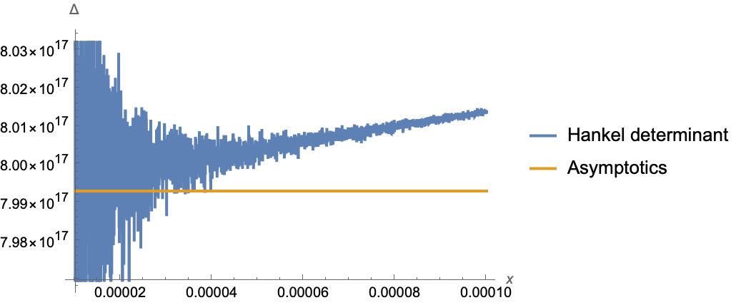
Figure 2. Plot of the expression $x^{50}\Delta_{n}(x,\alpha)$ and its small $x$ asymptotics for $n=10$ and $\alpha=0.98$, $d_{1}=0.55$, $d_{2}=0.71$.

Our result is useful for the numerical computation of solution $u_{n}(x,\alpha)$. If we try to naively use formula $\eqref{eq:q_n_formula}$, we would encounter large cancellation error in the computation of Hankel determinant, see Figure 2. Instead, we use the result of Theorem 1.2 and method of undetermined coefficients to derive detailed asymptotic expansion of solution $u_{n}(x,\alpha)$:

$$u_{n}(x,\alpha)\sim\sum_{k=0}^{\infty}\sum_{l=-k-1}^{k+1}(b_{kl}x^{2k+(2l-1)p}+c_{kl}x^{2k+1+2lp}),\quad x\to 0.$$ (6)

Here we denoted by $p$ the power of asymptotic of $u_{n}(x,\alpha)$ at zero: $u_{n}(x,\alpha)\sim ax^{p}$ as $x\to 0$ and $|\mathrm{Re}(p)|\leq 1$. Afterwards we can use truncated version of (6) to get precise initial condition of $u_{n}(x,\alpha)$ at some point near zero. Plugging this initial condition in the ODE solver we can determine values of $u_{n}(x,\alpha)$ away from zero. There is difficulty here, when we use standard solver, since $u_{n}(x,\alpha)$ has singularities on the real line. Instead we have to step in the complex plane to go around the singularity. For Painlevé III corresponding code was developed in [FFW18]. The authors generously shared it with us and we present the result in Figure 3. We observe that for large $n$ the pole structure is similar to the pole structure of rational solutions of Painlevé III equation observed in [BMS18], but the poles now lie also in the regions extending to infinity.

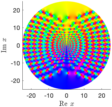
Figure 3. Complex plot of solution $u_{n}(x,\alpha)$, for $n=15$ and $\alpha=-\frac{223}{225}$, $d_{1}=0.55$, $d_{2}=0.71$.

2. Construction of Bessel function solutions of Painlevé III equation

2.1. The simultaneous solutions of Ricatti and Painlevé III equations

The standard way to construct the special function solutions of Painlevé equations is to use Ricatti equation, see [Cla23, Theorem 3.5] and [DLMF, §32.10(iii)]. More precisely, we look for the simultaneous solutions of Painlevé III equation (1) and the Ricatti equation

$$u^{\prime}(x)=a(x)u^{2}(x)+b(x)u(x)+c(x),\quad a(x)\neq 0.$$ (7)

Taking the first derivative of (7) and plugging in the $u^{\prime}(x)$, we get:

$$u^{\prime\prime}(x)=2a^{2}(x)u^{3}(x)+(a^{\prime}(x)+3a(x)b(x))u^{2}(x)+(2a(x)c(x)+b^{2}(x)+b^{\prime}(x))u(x)+(b(x)c(x)+c^{\prime}(x))$$

Meanwhile, plugging (7) into (1), we get:

$$u^{\prime\prime}(x)= (a^{2}(x)+1)u^{3}(x)+\left((2a(x)b(x)-\frac{a(x)-\alpha}{x}\right)u^{2}(x)+\left(b^{2}(x)+2a(x)c(x)-\frac{b(x)}{x}\right)u(x)$$

$$+\frac{c(x)-1}{u(x)}+2b(x)c(x)-\frac{c(x)-\beta}{x}.$$

By matching and solving for the coefficients, we have totally four cases. We list them below:

$$a(x)=1, b(x)=\frac{\alpha-1}{x}, c(x)=1, \beta=2-\alpha$$ (8)

$$a(x)=-1, b(x)=\frac{-1-\alpha}{x}, c(x)=-1, \beta=-2-\alpha$$ (9)

$$a(x)=1, b(x)=\frac{\alpha-1}{x}, c(x)=-1, \beta=\alpha-2$$ (10)

$$a(x)=-1, b(x)=\frac{-1-\alpha}{x}, c(x)=1, \beta=\alpha+2$$ (11)

Notice that if $u(x)$ solves the Ricatti equation, then $w(x)=\exp\left(-\int a(x)u(x)dx\right)$ solves the following linear ODE:

$$a(x)w^{\prime\prime}(x)-(a^{\prime}(x)+a(x)b(x))w^{\prime}(x)+c(x)a^{2}(x)w(x)=0,\quad a(x)\neq 0.$$ (12)

From now on we will only focus on the case (8). The equation (12) becomes

$$w{{}^{\prime\prime}}(x)+\frac{(1-\alpha)}{x}w{{}^{\prime}}(x)+w(x)=0.$$ (13)

We can notice that $x^{-\frac{\alpha}{2}}w(x)$ solves Bessel equation (108) with $\nu=\frac{\alpha}{2}$. For $\alpha\in\mathbb{C}\setminus(2\mathbb{Z}+i\mathbb{R})$ we denote the solution of (13)

$$w(x,\alpha)=x^{\frac{\alpha}{2}}\mathcal{C}_{\frac{\alpha}{2}}(x)$$ (14)

where cylinder function $\mathcal{C}_{\nu}(x)$ is given by (3). Here we assume that $\frac{\alpha}{2}$ is not integer for convenience in our future computations. As the result we get

Proposition 2.1 ([DLMF, §32.10(iii)]).

Painlevé III equation (1) with $\beta=2-\alpha$ and $\alpha\in\mathbb{C}\setminus(2\mathbb{Z}+i\mathbb{R})$ admits the special function solution

$$u_{0}(x,\alpha)=-\frac{d}{dx}\ln(w(x,\alpha)).$$ (15)

with $w(x,\alpha)$ given by (14).

Remark 2.1.

In the case (9) solution is also given in term of Bessel functions, while in the cases (10), (11) it is given in terms of modified Bessel functions.

2.2. Bäcklund transformation

To construct more solutions for PIII equation with more general parameters, we need to introduce a powerful tool. Bäcklund transformations for the Painlevé-III equation are given by (see [DLMF, §32.7(iii)])

$$B_{1}:(u(x),\alpha,\beta)\to\left(\frac{xu^{\prime}(x)+xu^{2}(x)-\beta u(x)-u(x)+x}{u(x)(xu^{\prime}(x)+xu^{2}(x)+\alpha u(x)+u(x)+x)},\alpha+2,\beta+2\right)$$ (16)

$$B_{2}:(u(x),\alpha,\beta)\to\left(-\frac{xu^{\prime}(x)-xu^{2}(x)-\beta u(x)-u(x)+x}{u(x)(xu^{\prime}(x)-xu^{2}(x)-\alpha u(x)+u(x)+x)},\alpha-2,\beta+2\right)$$ (17)

Assume that $u(x)$ solves Painlevé-III equation. Denote $B_{1}(u(x),\alpha,\beta)=(W(x),\alpha+2,\beta+2)$. One can show that $W(x)$ solves Painlevé-III equation

$$W^{\prime\prime}(x)=\dfrac{\left(W^{\prime}(x)\right)^{2}}{W(x)}-\dfrac{W^{\prime}(x)}{x}+\dfrac{(\alpha+2)W^{2}(x)+(\beta+2)}{x}+W^{3}(x)-\frac{1}{W(x)}.$$

Similarly, denote $B_{2}(u(x),\alpha,\beta)=(W(x),\alpha-2,\beta+2)$. One can show that $W(x)$ solves Painlevé-III equation

$$W^{\prime\prime}(x)=\dfrac{\left(W^{\prime}(x)\right)^{2}}{W(x)}-\dfrac{W^{\prime}(x)}{x}+\dfrac{(\alpha-2)W^{2}(x)+(\beta+2)}{x}+W^{3}(x)-\frac{1}{W(x)}.$$

Proposition 2.2 ([DLMF, §32.7(iii)]).

Denote $B_{1}^{n}(u_{0}(x,\alpha),\alpha,2-\alpha)=(u_{n}(x,\alpha),\alpha+2n,-\alpha+2+2n)$ with $u_{0}(x,\alpha)$ given by (15). Then $u_{n}(x,\alpha)$ is the special function solution of Painlevé III equation (5).

We can observe that parameters of Painlevé-III equation (5) parameters satisfy $\alpha+\beta\in 2+4\mathbb{N}$. We will use Bäcklund tranformation $B_{2}$ in our future constructions.

Remark 2.2.

Using the transformation $u(x)\rightarrow-u(x)$ we can get solutions with $\alpha+\beta\in-2-4\mathbb{N}$. Using the transformation $u(x)\rightarrow-iu(-ix)$ we can get solutions with $\alpha-\beta\in 2+4\mathbb{N}$.

3. Hankel determinants of cylinder functions

3.1. Hamiltonian system

We use the formulas presented in [Cla23].

Definition 3.1.

We define the momentum associated to the solution of Painlevé-III equation using formula

$$v(x)=\frac{1}{2u^{2}(x)}\left(xu^{\prime}(x)+xu^{2}(x)-x+u(x)\left({\beta-1}{}\right)\right)$$

Definition 3.2.

We define the Hamiltonian associated to the solution of Painlevé-III equation using formula

$$H(x)={v^{2}(x)}{}u^{2}(x)-v(x)\left(xu^{2}(x)-{x}+u(x)\left({\beta-1}\right)\right)+2xu(x)\left(\frac{\beta-(2+\alpha)}{4}\right)$$

One can show that Painlevé-III equation is equivalent to the Hamiltonian system:

$$x\dfrac{du}{dx}=\dfrac{\partial H}{\partial v},$$

$$\quad x\dfrac{dv}{dx}=-\dfrac{\partial H}{\partial u}.$$

3.2. Tau function and Toda equation

For details of this section see [Oka87] and [FW02].

Definition 3.3.

We define the auxiliary Hamiltonian associated to the solution of Painlevé-III equation using formula

$$h(x)=\frac{1}{2}\left(H(x)+u(x)v(x)-x^{2}+\frac{1}{4}(\beta-4)(\beta+(\alpha-2))\right).$$

In this section we will deal with generic solution $u(x)$. Since momentum, Hamiltonian and auxiliary Hamiltonian are expressed in terms of $u(x)$, the action of Bäcklund transformation $B_{1}$ can be extended to them by formulas $(u(x),\alpha,\beta)$ to $v(x)$, $H(x)$ and $h(x)$. We denote

$$(u_{n}(x),\alpha+2n,\beta+2n)=B_{1}^{n}(u(x),\alpha,\beta)$$ (18)

$$v_{n}(x)=\left.v(x)\right|_{u(x)\to u_{n}(x),\beta\to\beta+2n}$$ (19)

$$H_{n}(x)=\left.H(x)\right|_{u(x)\to u_{n}(x),v(x)\to v_{n}(x),\alpha\to\alpha+2n,\beta\to\beta+2n}$$ (20)

$$h_{n}(x)=\left.h(x)\right|_{H(x)\to H_{n}(x),u(x)\to u_{n}(x),v(x)\to v_{n}(x),\alpha\to\alpha+2n,\beta\to\beta+2n}$$ (21)

On the path to derive the representation of Proposition 1.1 we introduce the tau function associated with the solution $u(x)$.

Definition 3.4.

Define tau function associated to the solution of Painlevé-III equation using formula

$$x\dfrac{d}{dx}\ln(\tau_{n}(x))=h_{n}(x).$$ (22)

It is defined up to a multiplicative constant.

Proposition 3.1 ([FW02, Proposition 4.2]).

Tau function for Painlevé-III equation given by (22) satisfies Toda equation

$$x\dfrac{d}{dx}x\dfrac{d}{dx}\ln(\tau_{n}(x))=c_{n}\frac{\tau_{n+1}(x)\tau_{n-1}(x)}{\tau_{n}^{2}(x)}$$

for some constants $c_{n}$. Moreover, one can choose multiplicative constants in the definition (22) in such a way that $c_{n}=1$.

Proof.

Using the Bäcklund transformation $B_{1}$ we can check the identity

$$h_{n+1}(x)=h_{n}(x)-v_{n}u_{n}(x)-\frac{3}{2}+\frac{\alpha}{4}-\frac{3\beta}{4}+2n$$ (23)

Denote $A_{n}(x)=x\dfrac{d}{dx}x\dfrac{d}{dx}\ln(\tau_{n}(x))$ and $B_{n}(x)=\frac{\tau_{n+1}(x)\tau_{n-1}(x)}{\tau_{n}^{2}(x)}$. We want to show that $A_{n}(x)=c_{n}B_{n}(x)$. Taking natural log on both sides, we get $\ln A_{n}(x)=\ln B_{n}(x)+\ln c_{n}$. Therefore, it is sufficient to show

$$\dfrac{d}{dx}(\ln A_{n}(x)-\ln B_{n}(x))=0.$$ (24)

Well, by using Definition 3.4 and the identity (23), we have:

$$\dfrac{d}{dx}\ln(B_{n}(x))=\frac{v_{n-1}(x)u_{n-1}(x)-v_{n}(x)u_{n}(x)+2}{x}$$ (25)

$$\dfrac{d}{dx}\ln(A_{n}(x))=\frac{h^{\prime}_{n}(x)+xh^{\prime\prime}_{n}(x)}{xh^{\prime}_{n}(x)}$$ (26)

By using Definition 3.3 and (18)–(21), we rewrite (26), (25) in terms of $u_{n}(x)$. After a long computation we obtain (24).

Let’s show that using transformation $\tau_{n}(x)\to a_{n}\tau_{n}(x)$ one can make sure that the constant $c_{n}$ in the Toda equation is $1$. We notice that $a_{n}$ has to satisfy a difference equation

$$c_{n}a_{n}^{2}=a_{n+1}a_{n-1}.$$

Its general solution is given by

$$a_{n}=\frac{a_{1}^{n}}{a_{0}^{n-1}}\prod_{j=1}^{n-1}\prod_{i=1}^{j}c_{i},\ \ n\in\mathbb{N}$$

We can pick the initial conditions $a_{0}=a_{1}=1$ and choose

$$a_{n}=\prod_{j=1}^{n-1}\prod_{i=1}^{j}c_{i},\ \ n\in\mathbb{N}.$$

∎

3.3. Wronskian solutions of Toda equation

Toda equation determines the tau function recursively given initial conditions. If we want to derive some nice formula for it, we need some properties of determinants. The Leibniz formula for the determinant of $n\times n$ matrix $A=\left\{a_{ij}\right\}_{i,j=1}^{n}$ is given by

$$\det(A)=\sum_{\sigma\in S_{n}}\mathrm{sgn}(\sigma)\prod_{k=1}^{n}a_{k,\sigma(k)}$$

where $S_{n}$ is the set of permutations of $n$ elements and $\mathrm{sgn}(\sigma)$ is sign of permutation $\sigma$. Directly using the Leibniz formula above, we can show the following formulas for the derivative of a determinant

$$\dfrac{d}{dx}\det(A)=\sum_{j=1}^{n}\sum_{\sigma\in S_{n}}\mathrm{sgn}(\sigma)\left(\dfrac{d}{dx}a_{j,\sigma(j)}\right)\prod_{\begin{subarray}{c}k=1\\ k\neq j\end{subarray}}^{n}a_{k,\sigma(k)}$$ (27)

Remembering that $\det(A^{T})=\det(A)$ we can write the alternative formula

$$\dfrac{d}{dx}\det(A)=\sum_{j=1}^{n}\sum_{\sigma\in S_{n}}\mathrm{sgn}(\sigma)\left(\dfrac{d}{dx}a_{\sigma(j),j}\right)\prod_{\begin{subarray}{c}k=1\\ k\neq j\end{subarray}}^{n}a_{\sigma(k),k}.$$ (28)

Denote $A_{i|j}$ the matrix obtained from $A$ by deleting of $i$th row and $j$th column. The Laplace expansion for the determinant along the $j$th row is given by

$$\det(A)=\sum_{k=1}^{n}(-1)^{k+j}a_{jk}\det(A_{j|k})$$

Proposition 3.2 (see [VV23]).

Denote $A_{ij|kl}$ the matrix obtained from $A$ by deleting of $i$th and $j$th row anf $k$th and $l$th column. Determinats of these matrices satisfy Deshanot-Jacobi identity

$$\det(A)\det(A_{ij|ij})=\det(A_{i|i})\det(A_{j|j})-\det(A_{i|j})\det(A_{j|i}),\quad 1\leq i,j\leq n$$ (29)

Proposition 3.3 ([FW02, (2.43)]).

The sequence of functions

$$f_{n}(x)=\det\left(\left\{\left(x\dfrac{d}{dx}\right)^{i+j}f_{0}(x)\right\}_{i,j=0}^{n}\right)$$ (30)

solves Toda equation corresponding to Painlevé-III equation

$$\left(x\dfrac{d}{dx}\right)^{2}\ln(f_{n}(x))=\frac{f_{n+1}(x)f_{n-1}(x)}{f_{n}^{2}(x)},\quad n\geq 1.$$ (31)

Proof.

Specifically, to match the expression in Proposition 3.2, we rewrite (31) as:

$$f_{n-1}(x)f_{n+1}(x)=f_{n}(x)\left(x\dfrac{d}{dx}\right)^{2}f_{n}(x)-\left(x\dfrac{d}{dx}f_{n}(x)\right)^{2},\quad n\geq 1$$

Put $f_{n+1}(x)=\det(A)$. It follows that $f_{n}(x)=\det(A_{n+2|n+2})$ and $f_{n-1}(x)=\det(A_{n+1,n+2|n+1,n+2})$. We take the first derivative of the determinant in (30) by multi-linearity with respect to rows using (27). Since a determinant with two identical rows is zero, we end up with $x\dfrac{d}{dx}f_{n}(x)=\det(A_{n+1|n+2})$. Since $A_{n+1|n+2}=(A_{n+2|n+1})^{T}$, it implies that $x\dfrac{d}{dx}f_{n}(x)=\det(A_{n+1|n+2})=\det(A_{n+2|n+1})$. Then we take the second derivative of the determinant in (30) successively by multi-linearity with respect to columns using (28). Similarly, since a determinant with two identical columns is zero, we end up with $\left(x\dfrac{d}{dx}\right)^{2}f_{n}(x)=\det(A_{n+1|n+1})$. Using (29) we obtain (31). ∎

Now let’s return to the special function solutions $u_{n}(x,\alpha)$. We compute corresponding auxiliary Hamiltonians $h_{0}(x,\alpha)$, $h_{1}(x,\alpha)$, and $h_{2}(x,\alpha)$. It turns out that corresponding tau functions can be chosen as

$$\tau_{0}(x,\alpha)=1,$$ (32)

$$\tau_{1}(x,\alpha)=\mathcal{C}_{\frac{\alpha}{2}}(x),$$ (33)

$$\tau_{2}(x,\alpha)=\det\left(\begin{array}[]{cc}\tau_{1}(x,\alpha)&x\dfrac{d}{dx}\tau_{1}(x,\alpha)\vspace{0.2cm}\\ x\dfrac{d}{dx}\tau_{1}(x,\alpha)&\left(x\dfrac{d}{dx}\right)^{2}\tau_{1}(x,\alpha)\end{array}\right).$$ (34)

where $\mathcal{C}_{\nu}(x)$ is given by (3). Toda equation determines tau function uniquely given the initial condition. The solution with initial conditions (33), (34) is given by (30) by Proposition 3.3. As the result we get

Proposition 3.4.

Tau functions associated to the special function solutions $u_{n}(x,\alpha)$ can be chosen as

$$\tau_{n}(x,\alpha)=\det\left(\left\{\left(x\dfrac{d}{dx}\right)^{i+j-2}\tau_{1}(x,\alpha)\right\}_{i,j=1}^{n}\right)$$ (35)

with $\tau_{1}(x,\alpha)=\mathcal{C}_{\frac{\alpha}{2}}(x)$, $\tau_{0}(x,\alpha)=1$.

Proposition 3.5.

Fromula (35) can be alternatively written as

$$\tau_{n}(x,\alpha)=x^{n(n-1)}(-1)^{\frac{n(n-1)}{2}}\Delta_{n}(x,\alpha).$$ (36)

where $\Delta_{n}(x,\alpha)$ is given by (2).

Proof.

Using mathematical induction and identity (113) one can compute the structure of $\left(x\dfrac{d}{dx}\right)^{j}\mathcal{C}_{\frac{\alpha}{2}}(x)$:

$$\left(x\dfrac{d}{dx}\right)^{j}\mathcal{C}_{\frac{\alpha}{2}}(x)=x^{j}\mathcal{C}_{\frac{\alpha}{2}-j}(x)+\sum_{k=0}^{j-1}c_{kj}x^{k}\mathcal{C}_{\frac{\alpha}{2}-k}(x)$$ (37)

where $c_{kj}$ are constant coefficients. Well, we furtherly simplify the determinant using (37):

$$\det\left(\left\{\left(x\dfrac{d}{dx}\right)^{k+j}\mathcal{C}_{\frac{\alpha}{2}}(x)\right\}_{k,j=0}^{n-1}\right)$$

$$=\begin{vmatrix}\mathcal{C}_{\frac{\alpha}{2}}(x)&x\dfrac{d}{dx}\mathcal{C}_{\frac{\alpha}{2}}(x)&\cdots\\ x\mathcal{C}_{\frac{\alpha}{2}-1}(x)+c_{01}\mathcal{C}_{\frac{\alpha}{2}}(x)&x\dfrac{d}{dx}\left(x\mathcal{C}_{\frac{\alpha}{2}-1}(x)+c_{01}\mathcal{C}_{\frac{\alpha}{2}}(x)\right)&\cdots\\ x^{2}\mathcal{C}_{\frac{\alpha}{2}-2}(x)+c_{12}x\mathcal{C}_{\frac{\alpha}{2}-1}(x)+c_{02}\mathcal{C}_{\frac{\alpha}{2}}(x)&x\dfrac{d}{dx}\left(x^{2}\mathcal{C}_{\frac{\alpha}{2}-2}(x)+c_{12}\mathcal{C}_{\frac{\alpha}{2}-1}+c_{02}\mathcal{C}_{\frac{\alpha}{2}}(x)\right)&\cdots\\ \vdots&\vdots&\ddots\end{vmatrix}$$

Observe that by elementary row operations, we can always use the previous rows to eliminate the $\sum_{k=0}^{j-1}c_{kj}x^{k}\mathcal{C}_{\frac{\alpha}{2}-k}(x)$ part in a fixed row and the value of the determinant doesn’t change. Finally, we will end up with:

$$\det\left(\left\{\left(x\dfrac{d}{dx}\right)^{k+j}\mathcal{C}_{\frac{\alpha}{2}}(x)\right\}_{k,j=0}^{n-1}\right)$$

$$=\begin{vmatrix}\mathcal{C}_{\frac{\alpha}{2}}(x)&x\dfrac{d}{dx}\mathcal{C}_{\frac{\alpha}{2}}(x)&\cdots\vspace{0.2cm}\\ x\,\mathcal{C}_{\frac{\alpha}{2}-1}(x)&x\dfrac{d}{dx}(x\,\mathcal{C}_{\frac{\alpha}{2}-1}(x))&\cdots\vspace{0.2cm}\\ x^{2}\mathcal{C}_{\frac{\alpha}{2}-2}(x)&x\dfrac{d}{dx}(x^{2}\mathcal{C}_{\frac{\alpha}{2}-2}(x))&\cdots\\ \vdots&\vdots&\ddots\end{vmatrix}=\det\left(\left\{\left(x\dfrac{d}{dx}\right)^{k}x^{j}\mathcal{C}_{\frac{\alpha}{2}-j}\right\}_{k,j=0}^{n-1}\right)$$

By relation (114), by induction, we can show:

$$\left(x\dfrac{d}{dx}\right)^{k}x^{j}\mathcal{C}_{\frac{\alpha}{2}-j}(x) =(-1)^{k}x^{j+k}\mathcal{C}_{\frac{\alpha}{2}-j+k}(x)+\sum_{n=0}^{k-1}d_{nkj}x^{j+n}\mathcal{C}_{\frac{\alpha}{2}-j+n}(x)$$ (38)

To prove (38) by (114), we first fix $k=1$ and induct on $j$. We have

$$x\dfrac{d}{dx}x^{j}\mathcal{C}_{\frac{\alpha}{2}-j}(x)=-x^{j+1}\mathcal{C}_{\frac{\alpha}{2}-j+1}(x)+x^{j}\left(\frac{\alpha}{2}-j\right)\mathcal{C}_{\frac{\alpha}{2}-j}(x)+jx^{j}\mathcal{C}_{\frac{\alpha}{2}-j}(x)$$ (39)

$$=-x^{j+1}\mathcal{C}_{\frac{\alpha}{2}-j+1}(x)+x^{j}\frac{\alpha}{2}\mathcal{C}_{\frac{\alpha}{2}-j}(x)$$

After showing (39) we induct on $k$. We also can notice that coefficient depending in $j$ cancels in the right hand side of (39). It implies that $d_{nkj}$ actually doesn’t depend on $j$. So (38) can be written as

$$\left(x\dfrac{d}{dx}\right)^{k}x^{j}\mathcal{C}_{\frac{\alpha}{2}-j}(x) =(-1)^{k}x^{j+k}\mathcal{C}_{\frac{\alpha}{2}-j+k}(x)+\sum_{n=0}^{k-1}d_{nk}x^{j+n}\mathcal{C}_{\frac{\alpha}{2}-j+n}(x)$$ (40)

Again, we furtherly simplify the determinant by (40):

$$\det\left(\left\{\left(x\dfrac{d}{dx}\right)^{k+j}\mathcal{C}_{\frac{\alpha}{2}}(x)\right\}_{k,j=0}^{n-1}\right)=\begin{vmatrix}\mathcal{C}_{\frac{\alpha}{2}}(x)&-x\,\mathcal{C}_{\frac{\alpha}{2}+1}(x)+d_{01}\mathcal{C}_{\frac{\alpha}{2}}(x)&\cdots\\ x\,\mathcal{C}_{\frac{\alpha}{2}-1}(x)&-x^{2}\mathcal{C}_{\frac{\alpha}{2}}(x)+d_{01}x\,\mathcal{C}_{\frac{\alpha}{2}-1}(x)&\cdots\\ \vdots&\vdots&\ddots\end{vmatrix}$$

Similarly, by applying elementary column operations, we can always use the previous columns to eliminate the $\sum_{n=0}^{k-1}d_{nk}x^{j+n}\mathcal{C}_{\frac{\alpha}{2}-j+n}(x)$ part in a fixed column and the value of the determinant doesn’t change. Finally, we will end up with:

$$\det\left(\left\{\left(x\dfrac{d}{dx}\right)^{k+j}\mathcal{C}_{\frac{\alpha}{2}}(x)\right\}_{k,j=0}^{n-1}\right)=\det\left((-1)^{k}x^{j+k}\mathcal{C}_{\frac{\alpha}{2}-j+k}(x)\right)$$

By multi-linearity of determinant, we can factor out $(-1)^{k}x^{j+k}$ and reach the conclusion:

$$\tau_{n}(x,\alpha)=\det\left((-1)^{k}x^{j+k}\mathcal{C}_{\frac{\alpha}{2}-j+k}(x)\right)=x^{n(n-1)}(-1)^{\frac{n(n-1)}{2}}\Delta_{n}(x,\alpha)$$

where $\Delta_{n}(x,\alpha)$ is given by (2). That completes the proof. ∎

3.4. Proof of Proposition 1.1

.

We start with considering Bäcklund transformations $B_{1}$ and $B_{2}$. Using the explicit formulas (16), (17) and equation (1) we can show that these transformations commute: $B_{1}B_{2}=B_{2}B_{1}$.

Let’s consider now $B_{2}$ applied to special function solution (15). After using differential equation (13) for $w(x)$ we get

$$B_{2}(u_{0}(x,\alpha),\alpha,2-\alpha)[1]=\frac{2-\alpha}{x}+\frac{w(x)}{w^{\prime}(x)}=\frac{2-\alpha}{x}+\dfrac{1}{\dfrac{\alpha}{2x}+\dfrac{\mathcal{C}^{\prime}_{\frac{\alpha}{2}}(x)}{\mathcal{C}_{\frac{\alpha}{2}}(x)}}.$$

The use notation $[1]$ above for the first component of the output of Bäcklund transformation. We use (114) to get

$$B_{2}(u_{0}(x,\alpha),\alpha,2-\alpha)[1]=\frac{2-\alpha}{x}+\dfrac{\mathcal{C}_{\frac{\alpha}{2}}(x)}{\mathcal{C}_{\frac{\alpha}{2}-1}(x)}.$$

Using identity (113) we can rewrite it as

$$B_{2}(u_{0}(x,\alpha),\alpha,2-\alpha)[1]=\frac{2-\alpha}{2x}-\dfrac{\mathcal{C}^{\prime}_{\frac{\alpha}{2}-1}(x)}{\mathcal{C}_{\frac{\alpha}{2}-1}(x)}=-\dfrac{d}{dx}\ln(w(x,\alpha-2))=u_{0}(x,\alpha-2).$$ (41)

Now using commutativity of $B_{1}$ and $B_{2}$ we get

$$B_{2}(u_{n}(x,\alpha),\alpha+2n,-\alpha+2+2n)=B_{2}B_{1}^{n}(u_{0}(x,\alpha),\alpha,-\alpha+2)$$

$$=B_{1}^{n}(u_{0}(x,\alpha-2),\alpha-2,-\alpha+4)=(u_{n}(x,\alpha-2),\alpha-2+2n,-\alpha+4+2n).$$

Similarly we can show that

$$B_{1}B_{2}(u_{n}(x,\alpha),\alpha+2n,-\alpha+2+2n)=(u_{n+1}(x,\alpha-2),\alpha+2n,-\alpha+6+2n).$$ (42)

On the next step of our proof introduce the following sequence of functions

$$\widetilde{u}_{n}(x,\alpha)=-\frac{\tau_{n+1}(x,\alpha-2)\tau_{n}(x,\alpha)}{\tau_{n+1}(x,\alpha)\tau_{n}(x,\alpha-2)}.$$ (43)

Using the Toda equation (31) and the definition of tau function (22) we can see that

$$\widetilde{u}_{n+1}(x,\alpha)=\widetilde{u}_{n}(x,\alpha)\dfrac{\left(x\dfrac{d}{dx}\right)^{2}\ln(\tau_{n+1}(x,\alpha-2))}{\left(x\dfrac{d}{dx}\right)^{2}\ln(\tau_{n+1}(x,\alpha))}=\widetilde{u}_{n}(x,\alpha)\dfrac{\left(x\dfrac{d}{dx}\right)h_{n+1}(x,\alpha-2)}{\left(x\dfrac{d}{dx}\right)h_{n+1}(x,\alpha)}.$$ (44)

Using identity (42) and definition of $h_{n+1}(x,\alpha)$ we can express right hand side of (44) in terms of $u_{n}(x,\alpha)$. We also provide intermediate formulas

$$h_{n+1}(x,\alpha)= -\frac{1}{8u_{n}(x,\alpha)^{2}}\Big{[}u_{n}(x,\alpha)^{2}\left(\alpha^{2}-4n^{2}+2x^{2}+3\right)+2xu_{n}(x,\alpha)\left(\alpha-2n+u_{n}^{\prime}(x,\alpha)-2\right)\Big{.}$$ (45)

$$\Big{.}+2x(\alpha+2n+2)u_{n}(x,\alpha)^{3}-x^{2}\left(\left(u_{n}^{\prime}(x,\alpha)\right)^{2}-1\right)+x^{2}u_{n}(x,\alpha)^{4}\Big{]},$$ (46)

$$h_{n+1}(x,\alpha-2)= -\frac{1}{8u_{n}(x,\alpha)^{2}}\Big{[}u_{n}(x,\alpha)^{2}\left(a^{2}-4a-4n^{2}+2x^{2}+7\right)+x^{2}u_{n}(x,\alpha)^{4}$$ (47)

$$-2xu_{n}(x,\alpha)\left(-a+2n+u_{n}^{\prime}(x,\alpha)+4\right)+2x(a+2n)u_{n}(x,\alpha)^{3}-x^{2}\left(u_{n}^{\prime}(x,\alpha)^{2}-1\right)\Big{]}.$$ (48)

As the result we get

$$\widetilde{u}_{n+1}(x,\alpha)=\widetilde{u}_{n}(x,\alpha)\frac{(-3+\alpha+2n)u_{n}(x,\alpha)+xu_{n}^{2}(x,\alpha)+x+xu_{n}^{\prime}(x,\alpha)}{u_{n}^{2}(x,\alpha)((1+\alpha+2n)u_{n}(x,\alpha)+xu_{n}^{2}(x,\alpha)+x+xu_{n}^{\prime}(x,\alpha))}.$$ (49)

Using identity (113), initial conditions (32), (33) and definiton (43) we can observe that

$$\widetilde{u}_{0}(x,\alpha)=u_{0}(x,\alpha).$$ (50)

Using explicit formula (16) for Bäcklund transformation $B_{1}$, relation (49) and mathematical induction we get

$$\widetilde{u}_{n}(x,\alpha)=u_{n}(x,\alpha).$$ (51)

Finally using (36) we arrive to (4). ∎

4. Asymptotics of Hankel determinant

4.1. Andrèief identity

To prove our result we rewrite Hankel determinant (2) as multiple contour integral.

Proposition 4.1 (see [For19]).

Andrèief identity is given by the following formula

$$\intop_{\Gamma}\ldots\intop_{\Gamma}\det\left(\left\{f_{j}(x_{k})\right\}_{j,k=1}^{n}\right)\det\left(\left\{g_{j}(x_{k})\right\}_{j,k=1}^{n}\right)\prod_{k=1}^{n}h(x_{k})dx_{k}=n!\det\left(\left\{\intop_{\Gamma}f_{j}(x)g_{k}(x)h(x)dx\right\}_{j,k=1}^{n}\right)$$

We apply Andrèief identity and get the following result.

Theorem 4.1.

The Hankel determinat $\Delta_{n}(x,\alpha)$ given by (2) can be rewritten as

$$\Delta_{n}(x,\alpha)=\frac{1}{n!}\intop_{\Gamma_{1}\cup\Gamma_{2}}\ldots\intop_{\Gamma_{1}\cup\Gamma_{2}}\prod_{1\leq j<k\leq n}(t_{k}-t_{j})\left(\frac{1}{t_{k}}-\frac{1}{t_{j}}\right)\prod_{k=1}^{n}h(t_{k})dt_{k}$$ (52)

where

$$h(t)=\frac{e^{\frac{x}{2}\left(t-\frac{1}{t}\right)}}{2\pi it^{1+\frac{\alpha}{2}}}\left(\left(d_{1}+d_{2}\cot\left(\frac{\pi\alpha}{2}\right)\right)\chi_{\Gamma_{1}}(t)+d_{2}\csc\left(\frac{\pi\alpha}{2}\right)e^{\frac{i\pi\alpha}{2}}\chi_{\Gamma_{2}}(t)\right),$$

and contours of integration $\Gamma_{1}$, $\Gamma_{2}$ are shown on Figure 7. We use the notation $\chi_{\Gamma_{j}}(t)$ for the characteristic function of contour $\Gamma_{j}$. We assume $-\pi<\arg(t)<\pi$ on contour $\Gamma_{1}$ and $0<\arg(t)<2\pi$ on contour $\Gamma_{2}$.

Proof.

Using contour integral representation (112) we get

$$\mathcal{C}_{\frac{\alpha}{2}-j+k}(x)=\intop_{\Gamma_{1}\cup\Gamma_{2}}t^{-k}t^{j}h(t)dt$$

Put $g_{k}(t)=t^{-k}$ and $f_{j}(t)=t^{j}$. By Proposition 4.1, we get

$$\Delta_{n}(x,\alpha) =\frac{1}{n!}\intop_{\Gamma_{1}\cup\Gamma_{2}}\ldots\intop_{\Gamma_{1}\cup\Gamma_{2}}\det\left(\left\{f_{j}(t_{k})\right\}_{j,k=0}^{n-1}\right)\det\left(\left\{g_{j}(t_{k})\right\}_{j,k=0}^{n-1}\right)\prod_{k=0}^{n-1}h(t_{k})dt_{k}$$

$$=\frac{1}{n!}\intop_{\Gamma_{1}\cup\Gamma_{2}}\ldots\intop_{\Gamma_{3}\cup\Gamma_{4}}\det\left(\left\{t_{k}^{j}\right\}_{j,k=0}^{n-1}\right)\det\left(\left\{t_{k}^{-j}\right\}_{j,k=0}^{n-1}\right)\prod_{k=0}^{n-1}h(t_{k})dt_{k}$$

By the formula for the Vandermonde determinant (115) we can simplify the integrand and get

$$\det\left(\left\{t_{k}^{j}\right\}_{j,k=0}^{n-1}\right)=\prod_{0\leq j<k\leq n-1}(t_{k}-t_{j})$$

$$\det\left(\left\{t_{k}^{-j}\right\}_{j,k=0}^{n-1}\right)=\prod_{0\leq j<k\leq n-1}\left(\frac{1}{t_{k}}-\frac{1}{t_{j}}\right)$$

Thus, the explicit formula for $\Delta_{n}(x,\alpha)$ is given by:

$$\Delta_{n}(x,\alpha)=\frac{1}{n!}\intop_{\Gamma_{1}\cup\Gamma_{2}}\ldots\intop_{\Gamma_{1}\cup\Gamma_{2}}\prod_{0\leq j<k\leq n-1}(t_{k}-t_{j})\left(\frac{1}{t_{k}}-\frac{1}{t_{j}}\right)\prod_{k=0}^{n-1}h(t_{k})dt_{k}.$$

For convenience we shift the index of variables $t_{k}$.

∎

4.2. Basic strategies

Up to this point, we’ve got enough preparation to compute the asymptotics at zero. Our goal is to get asymptotics $\Delta_{n}(x,\alpha)\sim b(n)x^{a(n)}$ when $x\rightarrow 0$. It is reasonable expectation since Bessel function $J_{\nu}(x)$ admits series representation (109). We summarize several key ideas to achieve this goal:

• The contours $\Gamma_{1}$ and $\Gamma_{2}$ spread out to zero and infinity in the formula (52). We can’t put $x=0$ here without losing convergence of the integral.

• Expanding the product $\prod_{k=0}^{n-1}h(t_{k})$ in the integrand of (52) we get the expressions, where some of the variables $t_{k}$ will belong to contour $\Gamma_{1}$ and others will belong to $\Gamma_{2}$.

• We apply change of variables $t=\frac{2}{x}s$ to variables on contours $\Gamma_{1}$. The integrand will preserve exponential decay at infinity when we put $x=0$. On the other hand, we can apply change of variable $t=\frac{x}{2}s$ to variables on contours $\Gamma_{2}$. In this case the integrand will preserve exponential decay at zero when we put $x=0$.

4.3. Expanded formula for $\Delta_{n}(x,\alpha)$

Lemma 4.1.

Let $I$ denotes a subset of the set of indices $\{1,\ldots,n\}$, $r$ denotes its cardinality $|I|$ and $I^{c}$ denotes its complement. One can observe the following identity

$$\prod\limits_{k=1}^{n}(c_{1}\chi_{\Gamma_{1}}(t_{k})+c_{2}\chi_{\Gamma_{2}}(t_{k}))=\sum_{\begin{subarray}{c}I\subset\{1,...,n\}\\ \left|I\right|=r\end{subarray}}c_{1}^{r}c_{2}^{n-r}\prod_{k\in I}\chi_{\Gamma_{1}}(t_{k})\prod_{j\in I^{c}}\chi_{\Gamma_{2}}(t_{j}).$$

Now we apply Lemma 4.1 to the expression in Theorem 4.1 in order to convert the formula into a summation form and decouple the contours. Denote

$${}c_{1}=d_{1}+d_{2}\cot\left(\frac{\pi\alpha}{2}\right),\quad c_{2}=d_{2}\csc\left(\frac{\pi\alpha}{2}\right)e^{\frac{i\pi\alpha}{2}}.$$ (53)

We have

$$\Delta_{n}(x,\alpha)=\frac{(-1)^{\frac{n(n-1)}{2}}}{n!}\intop_{\Gamma_{1}\cup\Gamma_{2}}\ldots\intop_{\Gamma_{1}\cup\Gamma_{2}}\prod_{m=1}^{n}(c_{1}\chi_{\Gamma_{1}}(t_{m})+c_{2}\chi_{\Gamma_{2}}(t_{m}))\prod_{1\leq j<k\leq n}\frac{(t_{j}-t_{k})^{2}}{t_{j}t_{k}}\prod_{l=1}^{n}\frac{e^{\frac{x}{2}(t_{l}-\frac{1}{t_{l}})}}{2\pi it_{l}^{\frac{\alpha}{2}+1}}dt_{l}$$

$$= \frac{(-1)^{\frac{n(n-1)}{2}}}{n!}\intop_{\Gamma_{1}\cup\Gamma_{2}}\ldots\intop_{\Gamma_{1}\cup\Gamma_{2}}\sum_{\begin{subarray}{c}I\subset\{1,...,n\}\\ \left|I\right|=r\end{subarray}}c_{1}^{r}c_{2}^{n-r}\prod_{i\in I}\chi_{\Gamma_{1}}(t_{i})\prod_{j\in I^{c}}\chi_{\Gamma_{2}}(t_{j})\prod_{1\leq j<k\leq n}\frac{(t_{j}-t_{k})^{2}}{t_{j}t_{k}}\prod_{l=1}^{n}\frac{e^{\frac{x}{2}(t_{l}-\frac{1}{t_{l}})}}{2\pi it_{l}^{\frac{\alpha}{2}+1}}dt_{l}$$

$$= \frac{(-1)^{\frac{n(n-1)}{2}}}{(2\pi i)^{n}n!}\sum_{\begin{subarray}{c}I\subset\{1,...,n\}\\ \left|I\right|=r\end{subarray}}c_{1}^{r}c_{2}^{n-r}\intop_{\Gamma_{1}}\ldots\intop_{\Gamma_{1}}\intop_{\Gamma_{2}}\ldots\intop_{\Gamma_{2}}\sqrt{\prod_{\begin{subarray}{c}j\not=k\\ j,k\in I\end{subarray}}\frac{(t_{j}-t_{k})^{2}}{t_{j}t_{k}}}\sqrt{\prod_{\begin{subarray}{c}j\not=k\\ j,k\in I^{c}\end{subarray}}\frac{(t_{j}-t_{k})^{2}}{t_{j}t_{k}}}\sqrt{\prod_{\begin{subarray}{c}j\in I\\ k\in I^{c}\end{subarray}}\frac{(t_{j}-t_{k})^{2}}{t_{j}t_{k}}}$$

$$\sqrt{\prod_{\begin{subarray}{c}j\in I^{c}\\ k\in I\end{subarray}}\frac{(t_{j}-t_{k})^{2}}{t_{j}t_{k}}}\prod_{l\in I}\frac{e^{\frac{x}{2}(t_{l}-\frac{1}{t_{l}})}}{t_{l}^{\frac{\alpha}{2}+1}}dt_{l}\prod_{l\in I^{c}}\frac{e^{\frac{x}{2}(t_{l}-\frac{1}{t_{l}})}}{t_{l}^{\frac{\alpha}{2}+1}}dt_{l}$$

For $t_{k}\in I$, we use change of variable $t_{k}=\frac{2}{x}s_{k}$. On the other hand, for $t_{j}\in I^{c}$, we use change of variable $t_{j}=\frac{x}{2}s_{j}$. The formula above becomes

$$\Delta_{n}(x,\alpha)=\frac{(-1)^{\frac{n(n-1)}{2}}}{(2\pi i)^{n}n!}\sum_{\begin{subarray}{c}I\subset\{1,...,n\}\\ \left|I\right|=r\end{subarray}}c_{1}^{r}c_{2}^{n-r}\intop_{\Gamma_{1}}\ldots\intop_{\Gamma_{1}}\intop_{\Gamma_{2}}\ldots\intop_{\Gamma_{2}}\prod_{\begin{subarray}{c}j<k\\ j,k\in I\end{subarray}}\frac{(s_{j}-s_{k})^{2}}{s_{j}s_{k}}\prod_{\begin{subarray}{c}j<k\\ j,k\in I^{c}\end{subarray}}\frac{(s_{j}-s_{k})^{2}}{s_{j}s_{k}}$$

$$\prod_{\begin{subarray}{c}j\in I\\ k\in I^{c}\end{subarray}}\left(\frac{2}{x}\right)^{2}\frac{(s_{j}(1+O(x^{2}))^{2}}{s_{j}s_{k}}\prod_{l\in I}\frac{e^{s_{l}}(1+O(x^{2}))}{\left(\frac{2}{x}\right)^{\frac{\alpha}{2}+1}s_{l}^{\frac{\alpha}{2}+1}}\frac{2}{x}ds_{l}\prod_{l\in I^{c}}\frac{e^{-\frac{1}{s_{l}}}(1+O(x^{2}))}{s_{l}^{\frac{\alpha}{2}+1}\left(\frac{x}{2}\right)^{\frac{\alpha}{2}+1}}\frac{x}{2}ds_{l}$$

Group all the $\frac{2}{x}$ factors together and pull them out of the summation,

$$\Delta_{n}(x,\alpha)=\frac{(-1)^{\frac{n(n-1)}{2}}}{(2\pi i)^{n}n!}\sum_{\begin{subarray}{c}I\subset\{1,...,n\}\\ \left|I\right|=r\end{subarray}}c_{1}^{r}c_{2}^{n-r}\left(\frac{2}{x}\right)^{-\alpha r+2r(n-r)+\frac{\alpha n}{2}}\intop_{\Gamma_{1}}\ldots\intop_{\Gamma_{1}}\intop_{\Gamma_{2}}\ldots\intop_{\Gamma_{2}}\prod_{\begin{subarray}{c}j<k\\ j,k\in I\end{subarray}}\frac{(s_{j}-s_{k})^{2}}{s_{j}s_{k}}$$

$$\prod_{\begin{subarray}{c}j<k\\ j,k\in I^{c}\end{subarray}}\frac{(s_{j}-s_{k})^{2}}{s_{j}s_{k}}\prod_{\begin{subarray}{c}j\in I\\ k\in I^{c}\end{subarray}}\frac{(s_{j}(1+O(x^{2}))^{2}}{s_{j}s_{k}}\prod_{\begin{subarray}{c}l\in I\end{subarray}}\frac{e^{s_{l}}(1+O(x^{2}))}{s_{l}^{\frac{\alpha}{2}+1}}ds_{l}\prod_{\begin{subarray}{c}l\in I^{c}\end{subarray}}\frac{e^{-\frac{1}{s_{l}}}(1+O(x^{2}))}{s_{l}^{\frac{\alpha}{2}+1}}ds_{l}$$

We also want to group all the products of variable s together and separate the integrals based on different contours. We rewrite the following three parts,

$$\prod_{\begin{subarray}{c}j<k\\ j,k\in I\end{subarray}}\frac{(s_{j}-s_{k})^{2}}{s_{j}s_{k}}=\prod_{\begin{subarray}{c}j<k\\ j,k\in I\end{subarray}}(s_{j}-s_{k})^{2}\prod_{\begin{subarray}{c}j\not=k\\ j,k\in I\end{subarray}}\frac{1}{\sqrt{s_{j}s_{k}}}=\prod_{\begin{subarray}{c}j<k\\ j,k\in I\end{subarray}}(s_{j}-s_{k})^{2}\prod_{l\in I}s_{l}^{\gamma_{1}}$$ (54)

$$\prod_{\begin{subarray}{c}j<k\\ j,k\in I^{c}\end{subarray}}\frac{(s_{j}-s_{k})^{2}}{s_{j}s_{k}}=\prod_{\begin{subarray}{c}j<k\\ j,k\in I^{c}\end{subarray}}(s_{j}-s_{k})^{2}\prod_{\begin{subarray}{c}j\not=k\\ j,k\in I^{c}\end{subarray}}\frac{1}{\sqrt{s_{j}s_{k}}}=\prod_{\begin{subarray}{c}j<k\\ j,k\in I^{c}\end{subarray}}(s_{j}-s_{k})^{2}\prod_{l\in I^{c}}s_{l}^{\gamma_{2}}$$ (55)

$$\prod_{\begin{subarray}{c}j\in I\\ k\in I^{c}\end{subarray}}\frac{s_{j}}{s_{k}}=\prod_{l\in I}s_{l}^{\gamma_{3}}\prod_{l\in I^{c}}s_{l}^{\gamma_{4}}$$ (56)

To find $\gamma_{1}$ we can interpret the product in (54) as product a over all elements of $r\times r$ matrix except for the diagonal. Terms with $s_{j}$ appear along $j$th row and $j$th column, so there are $2(r-1)$ of them. Similar argument can be used for computation of $\gamma_{2}$, but the size of the matrix would be $(n-r)\times(n-r)$. Keeping in mind that we still have square root and introducing the power $-\frac{1}{2}$, then we get:

$$\gamma_{1}=-\frac{2(r-1)}{2}=1-r,$$

$$\gamma_{2}=-\frac{2(n-r-1)}{2}=-n+r+1.$$

To compute $\gamma_{3}$ and $\gamma_{4}$ we visualize the number of the $s$-factors using the following matrix

$$\left\{\dfrac{s_{j_{\alpha}}}{s_{k_{\beta}}}\right\}_{\begin{subarray}{c}1\leq\alpha\leq r\\ 1\leq\beta\leq n-r\end{subarray}}=\begin{pmatrix}\dfrac{s_{j_{1}}}{s_{k_{1}}}&\dfrac{s_{j_{1}}}{s_{k_{2}}}&\dfrac{s_{j_{1}}}{s_{k_{3}}}&\cdots\vspace{0.2cm}\\ \dfrac{s_{j_{2}}}{s_{k_{1}}}&\dfrac{s_{j_{2}}}{s_{k_{2}}}&\dfrac{s_{j_{2}}}{s_{k_{3}}}&\cdots\\ \vdots&\vdots&\vdots&\ddots\end{pmatrix}$$

We can observe that horizontally, for each $s_{j_{\alpha}}$, there are $(n-r)$ factors. Vertically, for each $s_{k_{\beta}}$ there are $-r$ factors. We get

$$\gamma_{3}=n-r,$$

$$\gamma_{4}=-r.$$

As the result we obtain the following expanded formula for $\Delta_{n}(x,\alpha)$

$$\Delta_{n}(x,\alpha)= \frac{(-1)^{\frac{n(n-1)}{2}}}{(2\pi i)^{n}n!}\sum_{\begin{subarray}{c}I\subset\{1,...,n\}\\ \left|I\right|=r\end{subarray}}c_{1}^{r}c_{2}^{n-r}\left(\frac{2}{x}\right)^{-\alpha r+2r(n-r)+\frac{\alpha n}{2}}(1+O(x^{2}))$$

$$\times\intop_{\Gamma_{1}}\ldots\intop_{\Gamma_{1}}\prod_{\begin{subarray}{c}j<k\\ j,k\in I\end{subarray}}(s_{j}-s_{k})^{2}\prod_{\begin{subarray}{c}l\in I\end{subarray}}e^{s_{l}}s_{l}^{-\frac{\alpha}{2}-2r+n}ds_{l}\intop_{\Gamma_{2}}\ldots\intop_{\Gamma_{2}}\prod_{\begin{subarray}{c}j<k\\ j,k\in I^{c}\end{subarray}}(s_{j}-s_{k})^{2}\prod_{\begin{subarray}{c}l\in I^{c}\end{subarray}}e^{-\frac{1}{s_{l}}}s_{l}^{-\frac{\alpha}{2}-n}ds_{l}$$

We can see that terms in the right hand side only depend on cardinality of $I$. Rewriting it, we get the following preliminary asymptotic formula for $\Delta_{n}(x,\alpha)$.

Lemma 4.2.

The Hankel determinant (2) admits the following $x\rightarrow 0$ asymptotics for fixed $d_{1},d_{2}\in\mathbb{C}$, $n\in\mathbb{N}\cup\{0\}$, $\alpha\in\mathbb{C}\setminus(2\mathbb{Z}+i\mathbb{R})$

$$\begin{split}&\Delta_{n}(x,\alpha)=\frac{(-1)^{\frac{n(n-1)}{2}}}{(2\pi i)^{n}}\sum_{r=0}^{n}\frac{c_{1}^{r}c_{2}^{n-r}}{r!(n-r)!}\left(\frac{2}{x}\right)^{-\alpha r+2r(n-r)+\frac{\alpha n}{2}}(1+O(x^{2}))\\ &\times\intop_{\Gamma_{1}}\ldots\intop_{\Gamma_{1}}\prod_{{1\leq j<k\leq r}}(s_{j}-s_{k})^{2}\prod_{l=1}^{r}e^{s_{l}}s_{l}^{-\frac{\alpha}{2}-2r+n}ds_{l}\intop_{\Gamma_{2}}\ldots\intop_{\Gamma_{2}}\prod_{{1\leq j<k\leq n-r}}(s_{j}-s_{k})^{2}\prod_{l=1}^{n-r}e^{-\frac{1}{s_{l}}}s_{l}^{-\frac{\alpha}{2}-n}ds_{l}.\end{split}$$ (57)

Coefficients $c_{1}$, $c_{2}$ are given by (53). Contours of integration $\Gamma_{1}$, $\Gamma_{2}$ are shown on Figure 7. We assume $-\pi<\arg(t)<\pi$ on contour $\Gamma_{1}$ and $0<\arg(t)<2\pi$ on contour $\Gamma_{2}$.

4.4. Proof of Theorem 1.1

The asymptotics of $\Delta_{n}(x,\alpha)$ is the leading term of the asymptotic formula (57). Denote the power of $x$ appearing in (57) as $p(r,\alpha,n)$:

$$p(r,\alpha,n)=\alpha r-\frac{n\alpha}{2}-2r(n-r).$$ (58)

We need to find the minimum of $\mathrm{Re}(p(r,\alpha,n))$ with respect to $r$. Introduce notation for the index which realizes this minimum

$$\mathop{\min}\limits_{\begin{subarray}{c}0\leq r\leq n\\ r\in\mathbb{N}\cup\{0\}\end{subarray}}\mathrm{Re}(p(r,\alpha,n))=p(r_{c}(\alpha,n),\alpha,n).$$ (59)

We have the following formula for it.

Lemma 4.3.

The critical index $r_{c}(\alpha,n)$ defined by (59) admits the following piecewise formula

$$r_{c}(\alpha,n)=\begin{cases}0&\text{if }\mathrm{Re}(\alpha)>2n-2\\ j&\text{if }2n-4j-2<\mathrm{Re}(\alpha)<2n-4j+2\\ &\text{ and }j=1,2,\ldots,n-1\\ n&\text{if }\mathrm{Re}(\alpha)<-2n+2\end{cases}$$ (60)

Proof.

Since $0\leq r\leq n$ and $r\in\mathbb{Z}$, so $p(r,\alpha,n)$ only takes values on that discrete set. It is clear that $\mathrm{Re}(p(r,\alpha,n))$ is an upward parabola in variable $r$ and it takes minimum value at $r_{\min}(n,\alpha)=\frac{2n-\mathrm{Re}(\alpha)}{4}$. We will discuss different cases of relative positions between $r_{\min}(\alpha,n)$ and $r_{c}(\alpha,n)$. If $r_{\min}(\alpha,n)\leq 0$, then $r_{c}(\alpha,n)=0$. If $r_{\min}(\alpha,n)\geq n$, then $r_{c}(\alpha,n)=n$. Let $0\leq j\leq n$ and $j\leq r_{\min}(\alpha,n)\leq j+1$. If $j\leq r_{\min}(\alpha,n)<j+\frac{1}{2}$, then $r_{c}(\alpha,n)=j$. If $j+\frac{1}{2}<r_{\min}(\alpha,n)\leq j+1$, then $r_{c}(\alpha,n)=j+1$. In other words,

• $r_{c}(\alpha,n)=0$ when $\frac{2n-\mathrm{Re}(\alpha)}{4}<\frac{1}{2}$,

• $r_{c}(\alpha,n)=j$ when $j-\frac{1}{2}<\frac{2n-\mathrm{Re}(\alpha)}{4}<j+\frac{1}{2}$ and $j=1,2,\ldots,n-1$,

• $r_{c}(\alpha,n)=n$ when $\frac{2n-\mathrm{Re}(\alpha)}{4}>n-\frac{1}{2}$.

These conditions can be rewritten as (60). ∎

Remark 4.1.

Floor function gives a more compact form for $r_{c}(\alpha,n)$. Indeed $\forall$ $0\leq j\leq n$, we know $r_{c}(\alpha,n)=j$ if and only if $j-\frac{1}{2}\leq\frac{n}{2}-\frac{\mathrm{Re}(\alpha)}{4}\leq j+\frac{1}{2}$ or $j\leq\frac{n}{2}-\frac{\mathrm{Re}(\alpha)}{4}+\frac{1}{2}\leq j+1$. Therefore

$$r_{c}(\alpha,n)=\begin{cases}n&\text{if }{\mathrm{Re}(\alpha)}{}<2-2n,\\ \lfloor\frac{n}{2}-\frac{\mathrm{Re}(\alpha)}{4}+\frac{1}{2}\rfloor&\text{if }2-2n<{\mathrm{Re}(\alpha)}{}<2n-2,\\ 0&\text{if }\mathrm{Re}(\alpha)>2n-2.\end{cases}$$

As the result we have

$$\begin{split}&\Delta_{n}(x,\alpha)\sim\frac{(-1)^{\frac{n(n-1)}{2}}}{(2\pi i)^{n}}\frac{c_{1}^{r_{c}}c_{2}^{n-r_{c}}}{r_{c}!(n-r_{c})!}\left(\frac{x}{2}\right)^{p(r_{c},\alpha,n)}\intop_{\Gamma_{1}}\ldots\intop_{\Gamma_{1}}\prod_{{1\leq j<k\leq r_{c}}}(s_{j}-s_{k})^{2}\prod_{l=1}^{r_{c}}e^{s_{l}}s_{l}^{-\frac{\alpha}{2}-2r_{c}+n}ds_{l}\\ &\times\intop_{\Gamma_{2}}\ldots\intop_{\Gamma_{2}}\prod_{{1\leq j<k\leq n-r_{c}}}(s_{j}-s_{k})^{2}\prod_{l=1}^{n-r_{c}}e^{-\frac{1}{s_{l}}}s_{l}^{-\frac{\alpha}{2}-n}ds_{l},\quad\text{ as }x\to 0.\end{split}$$ (61)

By Andrèief identity again, we have

$$\intop_{\Gamma_{1}}\ldots\intop_{\Gamma_{1}}\prod_{\begin{subarray}{c}1\leq j<k\leq r_{c}\end{subarray}}(s_{j}-s_{k})^{2}\prod_{\begin{subarray}{c}l=1\end{subarray}}^{r_{c}}e^{s_{l}}s_{l}^{-\frac{\alpha}{2}-2r_{c}+n}ds_{l}=r_{c}!\det\left(\left\{\intop_{\Gamma_{1}}s^{k+j}e^{s}s^{-\frac{\alpha}{2}-2r_{c}+n}ds\right\}_{j,k=0}^{r_{c}-1}\right)$$ (62)

$$\intop_{\Gamma_{2}}\ldots\intop_{\Gamma_{2}}\prod_{\begin{subarray}{c}1\leq j<k\leq n-r_{c}\end{subarray}}(s_{j}-s_{k})^{2}\prod_{l=1}^{n-r_{c}}e^{-\frac{1}{s_{l}}}s_{l}^{-\frac{\alpha}{2}-n}ds_{l}=(n-r_{c})!\det\left(\left\{\intop_{\Gamma_{2}}s^{k+j}e^{-\frac{1}{s}}s^{-\frac{\alpha}{2}-n}ds\right\}_{j,k=0}^{n-r_{c}-1}\right)$$ (63)

Notice that the two determinants above are Hankel determinants with weights $w_{1}(s)=e^{s}s^{-\frac{\alpha}{2}-2r_{c}+n}$ on contour $\Gamma_{1}$ and $w_{2}(s)=e^{-\frac{1}{s}}s^{-\frac{\alpha}{2}-n}$ on contour $\Gamma_{2}$ respectively. To evaluate (62), (63), we reduce them to Hankel determinants with the Laguerre weight $w(x)=e^{-x}x^{\alpha}$, $\mathrm{Re}(\alpha)>-1$ on the contour $\Gamma=[0,\infty)$. Denote

$$H_{1}(\alpha,n)=\intop_{\Gamma_{1}}\ldots\intop_{\Gamma_{1}}\prod_{\begin{subarray}{c}1\leq j<k\leq r_{c}\end{subarray}}(s_{j}-s_{k})^{2}\prod_{\begin{subarray}{c}l=1\end{subarray}}^{r_{c}}e^{s_{l}}s_{l}^{-\frac{\alpha}{2}-2r_{c}+n}ds_{l}$$ (64)

and

$$H_{2}(\alpha,n)=\intop_{\Gamma_{2}}\ldots\intop_{\Gamma_{2}}\prod_{\begin{subarray}{c}1\leq j<k\leq n-r_{c}\end{subarray}}(s_{j}-s_{k})^{2}\prod_{l=1}^{n-r_{c}}e^{-\frac{1}{s_{l}}}s_{l}^{-\frac{\alpha}{2}-n}ds_{l}.$$ (65)

In $H_{1}(\alpha,n)$, we make the change of variable $s=\widetilde{s}e^{-i\pi}$. More specifically the modulus and argument of the variable transform as

$$|s|=|\widetilde{s}|$$

$$\arg(s)=\arg(\widetilde{s})-\pi,\quad 0<\arg(\widetilde{s})<2\pi.$$

The contour $\Gamma_{1}$ becomes $\widetilde{\Gamma_{1}}$ as shown in the picture below.

Figure 4. Contour $\widetilde{\Gamma_{1}}$

Also notice that

$$s_{l}^{-\frac{\alpha}{2}-2r_{c}+n} =e^{(-\frac{\alpha}{2}-2r_{c}+n)\ln|s_{l}|+(-\frac{\alpha}{2}-2r_{c}+n)i\arg(s_{l})}$$

$$=e^{(-\frac{\alpha}{2}-2r_{c}+n)\ln|\widetilde{s_{l}}|+(-\frac{\alpha}{2}-2r_{c}+n)i(\arg(\widetilde{s_{l}})-\pi)}$$

$$=\widetilde{s_{l}}^{-\frac{\alpha}{2}-2r_{c}+n}e^{-i\pi(-\frac{\alpha}{2}-2r_{c}+n)}$$

As the result we have

$$H_{1}(\alpha,n) =\intop_{\widetilde{\Gamma_{1}}}\ldots\intop_{\widetilde{\Gamma_{1}}}\prod_{\begin{subarray}{c}1\leq j<k\leq r_{c}\end{subarray}}(\widetilde{s_{j}}-\widetilde{s_{k}})^{2}\prod_{l=1}^{r_{c}}e^{-\widetilde{s_{l}}}\widetilde{s_{l}}^{-\frac{\alpha}{2}-2r_{c}+n}e^{-i\pi(-\frac{\alpha}{2}-2r_{c}+n)}(-1)d\widetilde{s_{l}}$$

$$=(-1)^{r_{c}}(e^{-i\pi(-\frac{\alpha}{2}-2r_{c}+n)})^{r_{c}}\intop_{\widetilde{\Gamma_{1}}}\ldots\intop_{\widetilde{\Gamma_{1}}}\prod_{\begin{subarray}{c}1\leq j<k\leq r_{c}\end{subarray}}(\widetilde{s_{j}}-\widetilde{s_{k}})^{2}\prod_{\begin{subarray}{c}l=1\end{subarray}}^{r_{c}}e^{-\widetilde{s_{l}}}\widetilde{s_{l}}^{-\frac{\alpha}{2}-2r_{c}+n}d\widetilde{s_{l}}$$

To continue our evaluation we need the following Lemma.

Lemma 4.4.

Using the properties of power function we can show the following identity

$$\intop_{0}^{\infty}s^{j}e^{-s}s^{\gamma}ds=\frac{1}{e^{2\pi i\gamma}-1}\intop_{\widetilde{\Gamma_{1}}}s^{j}e^{-s}s^{\gamma}ds,\quad j\in\mathbb{Z},\quad j+\mathrm{Re}(\gamma)>-1.$$ (66)

With the aid of (66) we can rewrite our contour integrals in terms of real line integrals under the convergence condition $\mathrm{Re}(\alpha)<2n-2$.

$$H_{1}(\alpha,n) =(-1)^{r_{c}}(e^{-i\pi(-\frac{\alpha}{2}-2r_{c}+n)})^{r_{c}}(e^{2\pi i(-\frac{\alpha}{2}-2r_{c}+n)}-1)^{r_{c}}$$

$$\times\intop_{0}^{\infty}\ldots\intop_{0}^{\infty}\prod_{\begin{subarray}{c}1\leq j<k\leq r_{c}\end{subarray}}(\widetilde{s_{j}}-\widetilde{s_{k}})^{2}\prod_{\begin{subarray}{c}l=1\end{subarray}}^{r_{c}}e^{-\widetilde{s_{l}}}\widetilde{s_{l}}^{-\frac{\alpha}{2}-2r_{c}+n}d\widetilde{s_{l}}$$

By using Andrèief idenity we get

$$H_{1}(\alpha,n) =r_{c}!(-1)^{r_{c}}\left(2i\sin\left(\left(-\frac{\alpha}{2}-2r_{c}+n\right)\pi\right)\right)^{r_{c}}H_{L}\left(-\frac{\alpha}{2}-2r_{c}+n,r_{c}-1\right)$$

where $H_{L}(\gamma,k)$ denotes $(k+1)\times(k+1)$ Hankel determinant associated with weight $e^{-x}x^{\gamma}$ on the contour $\Gamma=[0,\infty)$. It was computed in Proposition E.3. Using this result we have for $\mathrm{Re}(\alpha)<2n-2$

$$H_{1}(\alpha,n)=r_{c}!(-1)^{nr_{c}}(2i)^{r_{c}}\sin^{r_{c}}\left(\frac{\pi\alpha}{2}\right)\frac{G\left(1+n-r_{c}-\frac{\alpha}{2}\right)G(r_{c}+1)}{G\left(1-\frac{\alpha}{2}-2r_{c}+n\right)}.$$ (67)

We can notice that left and right hand sides of (67) are entire functions of $\alpha$. Therefore by the uniqueness of analytic continuation we can say that (67) holds for all $\alpha\in\mathbb{C}$.

Similarly, in $H_{2}(\alpha,n)$, we put $s=\frac{1}{\widetilde{s}}$. Then the modulus and argument of the variable respectively transform as

$$|s|=\frac{1}{|\widetilde{s}|}$$

$$\arg(\widetilde{s})=-\arg(s),\quad-2\pi<\arg(\widetilde{s})<0$$

The contour $\Gamma_{2}$ becomes $\widetilde{\Gamma_{2}}$ as shown in the picture below.

Figure 5. Contour $\widetilde{\Gamma_{2}}$

The second multi-integral becomes

$$H_{2}(\alpha,n) =\intop_{\widetilde{\Gamma_{2}}}\ldots\intop_{\widetilde{\Gamma_{2}}}\prod_{\begin{subarray}{c}1\leq j<k\leq n-r_{c}\end{subarray}}\left(\frac{1}{\widetilde{s_{j}}}-\frac{1}{\widetilde{s_{k}}}\right)^{2}\prod_{\begin{subarray}{c}l=1\end{subarray}}^{n-r_{c}}e^{-\widetilde{s_{l}}}\widetilde{s_{l}}^{\frac{\alpha}{2}+n}\left(-\frac{1}{s_{l}^{2}}\right)d\widetilde{s_{l}}$$

$$=(-1)^{n-r_{c}}\intop_{\widetilde{\Gamma_{2}}}\ldots\intop_{\widetilde{\Gamma_{2}}}\prod_{\begin{subarray}{c}1\leq j<k\leq n-r_{c}\end{subarray}}\left(\frac{\widetilde{s_{j}}-\widetilde{s_{k}}}{\widetilde{s_{j}}\widetilde{s_{k}}}\right)^{2}\prod_{\begin{subarray}{c}l=1\end{subarray}}^{n-r_{c}}e^{-\widetilde{s_{l}}}\widetilde{s_{l}}^{\frac{\alpha}{2}+n-2}d\widetilde{s_{l}}$$

$$=(-1)^{n-r_{c}}\intop_{\widetilde{\Gamma_{2}}}\ldots\intop_{\widetilde{\Gamma_{2}}}\prod_{\begin{subarray}{c}1\leq j<k\leq n-r_{c}\end{subarray}}(\widetilde{s_{j}}-\widetilde{s_{k}})^{2}\prod_{\begin{subarray}{c}l=1\end{subarray}}^{n-r_{c}}\widetilde{s_{l}}^{2r_{c}+2-2n}e^{-\widetilde{s_{l}}}\widetilde{s_{l}}^{\frac{\alpha}{2}+n-2}d\widetilde{s_{l}}$$

$$=(-1)^{n-r_{c}}\intop_{\widetilde{\Gamma_{2}}}\ldots\intop_{\widetilde{\Gamma_{2}}}\prod_{\begin{subarray}{c}1\leq j<k\leq n-r_{c}\end{subarray}}(\widetilde{s_{j}}-\widetilde{s_{k}})^{2}\prod_{\begin{subarray}{c}l=1\end{subarray}}^{n-r_{c}}e^{-\widetilde{s_{l}}}\widetilde{s_{l}}^{\frac{\alpha}{2}+2r_{c}-n}d\widetilde{s_{l}}$$

Here we used the square of (55)

$$\prod_{\begin{subarray}{c}1\leq j<k\leq n-r_{c}\end{subarray}}\left(\frac{\widetilde{s_{j}}-\widetilde{s_{k}}}{\widetilde{s_{j}}\widetilde{s_{k}}}\right)^{2}=\prod_{\begin{subarray}{c}1\leq j<k\leq n-r_{c}\end{subarray}}(\widetilde{s_{j}}-\widetilde{s_{k}})^{2}\prod_{\begin{subarray}{c}j\not=k\\ 1\leq j,k\leq n-r_{c}\end{subarray}}\frac{1}{\widetilde{s_{j}}\widetilde{s_{k}}}=\prod_{\begin{subarray}{c}1\leq j<k\leq n-r_{c}\end{subarray}}(\widetilde{s_{j}}-\widetilde{s_{k}})^{2}\prod_{l=1}^{n-r_{c}}\widetilde{s_{l}}^{2r_{c}+2-2n}$$

To continue our evaluation we need the following analog of Lemma 4.4.

Lemma 4.5.

Using the properties of power function we can show the following identity

$$\intop_{0}^{\infty}s^{j}e^{-s}s^{\gamma}ds=\frac{1}{1-e^{-2\pi i\gamma}}\intop_{\widetilde{\Gamma_{2}}}s^{j}e^{-s}s^{\gamma}ds,\quad j\in\mathbb{Z},\quad j+\mathrm{Re}(\gamma)>-1.$$ (68)

With the aid of (68) we can rewrite our contour integrals in terms of real line integrals under the convergence condition $\mathrm{Re}(\alpha)>2-2n$

$$H_{2}(\alpha,n) =(-1)^{n-r_{c}}\intop_{\widetilde{\Gamma_{2}}}\ldots\intop_{\widetilde{\Gamma_{2}}}\prod_{\begin{subarray}{c}1\leq j<k\leq n-r_{c}\end{subarray}}(\widetilde{s_{j}}-\widetilde{s_{k}})^{2}\prod_{\begin{subarray}{c}l=1\end{subarray}}^{n-r_{c}}e^{-\widetilde{s_{l}}}\widetilde{s_{l}}^{\frac{\alpha}{2}+2r_{c}-n}d\widetilde{s_{l}}$$ (69)

$$=(-1)^{n-r_{c}}(1-e^{-2\pi i(\frac{\alpha}{2}+2r_{c}-n)})^{n-r_{c}}\intop_{0}^{\infty}\ldots\intop_{0}^{\infty}\prod_{1\leq j<k\leq n-r_{c}}(\widetilde{s_{j}}-\widetilde{s_{k}})^{2}\prod_{\begin{subarray}{c}l=1\end{subarray}}^{n-r_{c}}e^{-\widetilde{s_{l}}}\widetilde{s_{l}}^{\frac{\alpha}{2}+2r_{c}-n}d\widetilde{s_{l}}$$ (70)

Using Andrèief identity we get

$$H_{2}(\alpha,n) =(n-r_{c})!(-1)^{n-r_{c}}(e^{-\pi i(\frac{\alpha}{2}+2r_{c}-n)})^{n-r_{c}}\left(2i\sin\left(\left(\frac{\alpha}{2}+2r_{c}-n\right)\pi\right)\right)^{n-r_{c}}$$

$$\times H_{L}\left(\frac{\alpha}{2}+2r_{c}-n,{n-r_{c}-1}\right).$$

We use Proposition E.3 to evaluate the Hankel determinant with Laguerre weight and arrive to the formula

$$H_{2}(\alpha,n)=(n-r_{c})!(-1)^{n-r_{c}}e^{-i\pi(n-r_{c})\frac{\alpha}{2}}(2i)^{n-r_{c}}\sin^{n-r_{c}}\left(\frac{\pi\alpha}{2}\right)\frac{{G(\frac{\alpha}{2}+r_{c}+1)}G(n+1-r_{c})}{G(\frac{\alpha}{2}+2r_{c}-n+1)}$$ (71)

We repeat the uniqueness of analytic continuation argument above to claim that formula (71) holds for all $\alpha\in\mathbb{C}$. Combining (67),(71), (57) and the definitions (64), (65) we get

$$\begin{split}&\Delta_{n}(x,\alpha)\sim\frac{(-1)^{\frac{n(n-1)}{2}}}{\pi^{n}}{c_{1}^{r_{c}}c_{2}^{n-r_{c}}}\left(\frac{x}{2}\right)^{p(r_{c},\alpha,n)}(-1)^{n-r_{c}+nr_{c}}e^{-i\pi(n-r_{c})\frac{\alpha}{2}}\sin^{n}\left(\frac{\pi\alpha}{2}\right)\\ &\frac{{G(\frac{\alpha}{2}+r_{c}+1)}G(n+1-r_{c})G\left(1+n-r_{c}-\frac{\alpha}{2}\right)G(r_{c}+1)}{G(\frac{\alpha}{2}+2r_{c}-n+1)G\left(1-\frac{\alpha}{2}-2r_{c}+n\right)},\quad\text{ as }x\to 0.\end{split}$$ (72)

Using definitions (58), (53) and formula (60) we finish the Proof of Theorem 1.1.

5. Asymptotics of special function solutions

To deduce the asymptotics of $u_{n}(x,\alpha)$, we need to use our main result Theorem 1.1 and Proposition 1.1. We have to shift the index of Hankel determinant $n$ and the parameter $\alpha$.

5.1. Piecewise function for the power of $x$ in the asymptotic of $u_{n}(x,\alpha)$.

Let’s introduce notation for the power of $x$ in the asymptotic of $\Delta_{n}(x,\alpha)$ in Theorem 1.1

$$p_{c}(\alpha,n)=p(r_{c}(\alpha,n),\alpha,n)=\begin{cases}-\frac{\alpha n}{2},&\text{ if }\mathrm{Re}(\alpha)>2n-2,\\ (\alpha-2n+2j)j-\frac{\alpha n}{2},&\text{ if }2n-4j-2<\mathrm{Re}(\alpha)<2n-4j+2,\\ &\text{ for }{j=1,\ldots,n-1}\\ \frac{\alpha n}{2},&\text{ if }\mathrm{Re}(\alpha)<-2n+2\end{cases}$$ (73)

Then the power of $x$ in the asymptotic of $u_{n}(x,\alpha)$ based on Proposition 1.1 is given by

$$e(\alpha,n)=p_{c}(\alpha-2,n+1)-p_{c}(\alpha-2,n)+p_{c}(\alpha,n)-p_{c}(\alpha,n+1).$$ (74)

Lemma 5.1.

The piecewise function for the power of $x$ in the asymptotic of $u_{n}(x,\alpha)$ is given by

$$e(\alpha,n)=\begin{cases}1&\text{if }\mathrm{Re}(\alpha)>2+2n\\ \alpha-2n+4j-1&\text{if }2n-4j<\mathrm{Re}(\alpha)<2n-4j+2\text{ and }j=0,1,\ldots,n\\ -\alpha+2n-4j-1&\text{if }2n-4j-2<\mathrm{Re}(\alpha)<2n-4j\text{ and }j=0,1,\ldots,n-1\\ -1&\text{if }\mathrm{Re}(\alpha)<-2n\end{cases}$$

Proof.

We plug in formula (73) in the expression (74).
If $\mathrm{Re}(\alpha)>2+2n$, then we have

$$p_{c}(\alpha,n)=-\frac{\alpha n}{2}, p_{c}(\alpha,n+1)=-\frac{\alpha n}{2}-\frac{\alpha}{2},$$ (75)

$$p_{c}(\alpha-2,n)={-\frac{\alpha n}{2}+n}, p_{c}(\alpha-2,n+1)=-\frac{\alpha n}{2}+n+1-\frac{\alpha}{2}.$$ (76)

That confirms first case. Similarly, if $2n-4j<\mathrm{Re}(\alpha)<2n-4j+2$ and $j=0,1,\ldots,n$, then we have:

$$p_{c}(\alpha,n)=(\alpha-2n+2j)j-\frac{\alpha n}{2},$$

$$p_{c}(\alpha,n+1)=(\alpha-2n+2j)j-2j-\frac{\alpha n}{2}-\frac{\alpha}{2},$$

$$p_{c}(\alpha-2,n)=(\alpha-2n+2j)j-2j-\frac{\alpha n}{2}+n,$$

$$p_{c}(\alpha-2,n+1)=(\alpha-2n+2j)j-\frac{\alpha n}{2}-n-1+\frac{\alpha}{2}.$$

Notice that for $p_{c}(\alpha-2,n+1)$ we had to shift index $j$ to $j+1$ in (73) to get correct formula. We confirmed the second case. If $2n-4j-2<\mathrm{Re}(\alpha)<2n-4j$ and $j=0,1,\ldots,n-1$, then we have

$$p_{c}(\alpha,n)=(\alpha-2n+2j)j-\frac{\alpha n}{2},$$

$$p_{c}(\alpha,n+1)=(\alpha-2n+2j)j-2n+2j-\frac{\alpha n}{2}+\frac{\alpha}{2},$$

$$p_{c}(\alpha-2,n)=(\alpha-2n+2j)j+\alpha-n+2j-\frac{\alpha n}{2},$$

$$p_{c}(\alpha-2,n+1)=(\alpha-2n+2j)j-\frac{\alpha n}{2}-n-1+\frac{\alpha}{2}.$$

Notice that now we had to shift index $j$ to $j+1$ in (73) for $p_{c}(\alpha-2,n+1)$, $p_{c}(\alpha,n+1)$, and $p_{c}(\alpha-2,n)$ to get correct formula. We confirmed the third case. Finally if $\mathrm{Re}(\alpha)<-2n$, then all terms in (74) change sign compared to the case $\mathrm{Re}(\alpha)>2n-2$. That confirms the last case and finishes the proof of Lemma 5.1. ∎

5.2. Proof of Theorem 1.2

In this part, we will compute the coefficients in the asymptotics of Theorem 1.2. We introduce notation for the coefficient in the asymptotics of $\Delta_{n}(x,\alpha)$ in Theorem 1.1. We included factor of $2$ inside of power of $x$ for convenience

$$c(\alpha,n)=\begin{cases}(-1)^{\frac{n(n+1)}{2}}\left(\frac{d_{2}}{\pi}\right)^{n}\frac{G(n+1)G(\frac{\alpha}{2}+1)}{G(\frac{\alpha}{2}-n+1)},&\text{ if }\mathrm{Re}(\alpha)>2n-2,\\ \\ (-1)^{\frac{n(n-1)}{2}+nj+n-j}\left(\frac{d_{2}}{\pi}\right)^{n}\left(\frac{d_{1}}{d_{2}}\sin\left(\frac{\pi\alpha}{2}\right)+\cos\left(\frac{\pi\alpha}{2}\right)\right)^{j}&\text{ if }2n-4j-2<\mathrm{Re}(\alpha)<2n-4j+2,\\ \times\frac{G(n-j+1)G(-\frac{\alpha}{2}+n-j+1)G(j+1)G(j+\frac{\alpha}{2}+1)}{G(-\frac{\alpha}{2}+n-2j+1)G(\frac{\alpha}{2}-n+2j+1)},&\text{ for }{j=1,\ldots,n-1}\\ \\ \frac{(-1)^{\frac{n(n-1)}{2}+n^{2}}}{\pi^{n}}\left(d_{1}\sin\left(\frac{\pi\alpha}{2}\right)+d_{2}\cos\left(\frac{\pi\alpha}{2}\right)\right)^{n}&\text{ if }\mathrm{Re}(\alpha)<-2n+2\\ \times\frac{G(n+1)G(-\frac{\alpha}{2}+1)}{G(-\frac{\alpha}{2}-n+1)},\end{cases}$$ (77)

Let’s denote the constant coefficient in the asymptotic of $u_{n}(x,\alpha)$ as $q(\alpha,n)$. We have

$$q(\alpha,n)=-\frac{c(\alpha-2,n+1)c(\alpha,n)}{c(\alpha-2,n)c(\alpha,n+1)}.$$ (78)

Lemma 5.2.

The piecewise formula for $q(\alpha,n)$ is given by

$$q(\alpha,n)=\begin{cases}\frac{2}{2n+2-\alpha},&\text{ if }\mathrm{Re}(\alpha)>2n+2,\\ \\ (-1)^{n}\left(\frac{d_{1}}{d_{2}}\sin\left(\frac{\pi\alpha}{2}\right)+\cos\left(\frac{\pi\alpha}{2}\right)\right)\left(\frac{\Gamma(-\frac{\alpha}{2}+n-2j+1)}{\Gamma(\frac{\alpha}{2}-n+2j)}\right)^{2}&\text{ if }2n-4j<\mathrm{Re}(\alpha)<2n-4j+2,\\ \times\frac{\Gamma(j+\frac{\alpha}{2})\Gamma(j+1)}{\Gamma(-\frac{\alpha}{2}+n-j+1)\Gamma(n-j+1)},&\text{ for }{j=0,\ldots,n}\\ \\ (-1)^{n}\left(\frac{d_{1}}{d_{2}}\sin\left(\frac{\pi\alpha}{2}\right)+\cos\left(\frac{\pi\alpha}{2}\right)\right)^{-1}\left(\frac{\Gamma(\frac{\alpha}{2}-n+2j+1)}{\Gamma(-\frac{\alpha}{2}+n-2j)}\right)^{2}&\text{ if }2n-4j-2<\mathrm{Re}(\alpha)<2n-4j,\\ \times\frac{\Gamma(-\frac{\alpha}{2}+n-j+1)\Gamma(n-j)}{\Gamma(j+\frac{\alpha}{2}+1)\Gamma(j+1)},&\text{ for }{j=0,\ldots,n-1}\\ \\ -\frac{\alpha}{2}-n&\text{ if }\mathrm{Re}(\alpha)<-2n\end{cases}$$ (79)

Proof.

For $\mathrm{Re}(\alpha)>2n+2$ we have

$$c(\alpha,n) =(-1)^{\frac{n(n+1)}{2}}\left(\frac{d_{2}}{\pi}\right)^{n}\frac{G(n+1)G(\frac{\alpha}{2}+1)}{G(\frac{\alpha}{2}-n+1)},$$ (80)

$$c(\alpha-2,n) =(-1)^{\frac{n(n+1)}{2}}\left(\frac{d_{2}}{\pi}\right)^{n}\frac{G(n+1)G(\frac{\alpha}{2}+1)}{G(\frac{\alpha}{2}-n+1)}\frac{\Gamma(\frac{\alpha}{2}-n)}{\Gamma(\frac{\alpha}{2})},$$ (81)

$$c(\alpha,n+1) =(-1)^{\frac{(n+2)(n+1)}{2}}\left(\frac{d_{2}}{\pi}\right)^{n+1}\frac{G(n+1)G(\frac{\alpha}{2}+1)}{G(\frac{\alpha}{2}-n+1)}{\Gamma(n+1)}{\Gamma\left(\frac{\alpha}{2}-n\right)},$$ (82)

$$c(\alpha-2,n+1) =(-1)^{\frac{(n+2)(n+1)}{2}}\left(\frac{d_{2}}{\pi}\right)^{n+1}\frac{G(n+1)G(\frac{\alpha}{2}+1)}{G(\frac{\alpha}{2}-n+1)}\frac{\Gamma(n+1)\Gamma\left(\frac{\alpha}{2}-n\right)\Gamma\left(\frac{\alpha}{2}-n-1\right)}{\Gamma\left(\frac{\alpha}{2}\right).}$$ (83)

That implies

$$q(\alpha,n)=-\frac{\Gamma\left(\frac{\alpha}{2}-n-1\right)}{\Gamma\left(\frac{\alpha}{2}-n\right)}=\frac{2}{2n+2-\alpha}.$$ (84)

That confirms the first case.

For $2n-4j<\mathrm{Re}(\alpha)<2n-4j+2$ we have

$$c(\alpha,n)=(-1)^{\frac{n(n-1)}{2}+nj+n-j}\left(\frac{d_{2}}{\pi}\right)^{n}\left(\frac{d_{1}}{d_{2}}\sin\left(\frac{\pi\alpha}{2}\right)+\cos\left(\frac{\pi\alpha}{2}\right)\right)^{j}$$ (85)

$$\times\frac{G(n-j+1)G(-\frac{\alpha}{2}+n-j+1)G(j+1)G(j+\frac{\alpha}{2}+1)}{G(-\frac{\alpha}{2}+n-2j+1)G(\frac{\alpha}{2}-n+2j+1)},$$ (86)

$$c(\alpha-2,n)=(-1)^{\frac{n(n-1)}{2}+nj+n}\left(\frac{d_{2}}{\pi}\right)^{n}\left(\frac{d_{1}}{d_{2}}\sin\left(\frac{\pi\alpha}{2}\right)+\cos\left(\frac{\pi\alpha}{2}\right)\right)^{j}$$ (87)

$$\times\frac{G(n-j+1)G(-\frac{\alpha}{2}+n-j+1)G(j+1)G(j+\frac{\alpha}{2}+1)}{G(-\frac{\alpha}{2}+n-2j+1)G(\frac{\alpha}{2}-n+2j+1)}\frac{\Gamma(-\frac{\alpha}{2}+n-j+1)\Gamma(\frac{\alpha}{2}-n+2j)}{\Gamma(j+\frac{\alpha}{2})\Gamma(-\frac{\alpha}{2}+n-2j+1)},$$ (88)

$$c(\alpha,n+1)=(-1)^{\frac{n(n+1)}{2}+nj+n+1}\left(\frac{d_{2}}{\pi}\right)^{n+1}\left(\frac{d_{1}}{d_{2}}\sin\left(\frac{\pi\alpha}{2}\right)+\cos\left(\frac{\pi\alpha}{2}\right)\right)^{j}$$ (89)

$$\times\frac{G(n-j+1)G(-\frac{\alpha}{2}+n-j+1)G(j+1)G(j+\frac{\alpha}{2}+1)}{G(-\frac{\alpha}{2}+n-2j+1)G(\frac{\alpha}{2}-n+2j+1)}\frac{\Gamma(-\frac{\alpha}{2}+n-j+1)\Gamma(n-j+1)\Gamma(\frac{\alpha}{2}-n+2j)}{\Gamma(-\frac{\alpha}{2}+n-2j+1)},$$ (90)

$$c(\alpha-2,n+1)=(-1)^{\frac{n(n+1)}{2}+nj+j+2n+2}\left(\frac{d_{2}}{\pi}\right)^{n+1}\left(\frac{d_{1}}{d_{2}}\sin\left(\frac{\pi\alpha}{2}\right)+\cos\left(\frac{\pi\alpha}{2}\right)\right)^{j+1}$$ (91)

$$\times\frac{G(n-j+1)G(-\frac{\alpha}{2}+n-j+1)G(j+1)G(j+\frac{\alpha}{2}+1)}{G(-\frac{\alpha}{2}+n-2j+1)G(\frac{\alpha}{2}-n+2j+1)}{\Gamma(j+1)\Gamma\left(-\frac{\alpha}{2}+n-j+1\right)}{}.$$ (92)

Combining these formulas we confirm the second case. Notice that for $c(\alpha-2,n+1)$ we had to shift index $j$ to $j+1$ in (77) to get correct formula.

For $2n-4j-2<\mathrm{Re}(\alpha)<2n-4j$ we have

$$c(\alpha,n)=(-1)^{\frac{n(n-1)}{2}+nj+n-j}\left(\frac{d_{2}}{\pi}\right)^{n}\left(\frac{d_{1}}{d_{2}}\sin\left(\frac{\pi\alpha}{2}\right)+\cos\left(\frac{\pi\alpha}{2}\right)\right)^{j}$$ (93)

$$\times\frac{G(n-j+1)G(-\frac{\alpha}{2}+n-j+1)G(j+1)G(j+\frac{\alpha}{2}+1)}{G(-\frac{\alpha}{2}+n-2j+1)G(\frac{\alpha}{2}-n+2j+1)},$$ (94)

$$c(\alpha-2,n)=(-1)^{\frac{n(n-1)}{2}+nj+2n}\left(\frac{d_{2}}{\pi}\right)^{n}\left(\frac{d_{1}}{d_{2}}\sin\left(\frac{\pi\alpha}{2}\right)+\cos\left(\frac{\pi\alpha}{2}\right)\right)^{j+1}$$ (95)

$$\times\frac{G(n-j+1)G(-\frac{\alpha}{2}+n-j+1)G(j+1)G(j+\frac{\alpha}{2}+1)}{G(-\frac{\alpha}{2}+n-2j+1)G(\frac{\alpha}{2}-n+2j+1)}\frac{\Gamma(j+1)\Gamma(-\frac{\alpha}{2}+n-2j)}{\Gamma(n-j)\Gamma(\frac{\alpha}{2}-n+2j+1)},$$ (96)

$$c(\alpha,n+1)=(-1)^{\frac{n(n+1)}{2}+nj+2n+1}\left(\frac{d_{2}}{\pi}\right)^{n+1}\left(\frac{d_{1}}{d_{2}}\sin\left(\frac{\pi\alpha}{2}\right)+\cos\left(\frac{\pi\alpha}{2}\right)\right)^{j+1}$$ (97)

$$\times\frac{G(n-j+1)G(-\frac{\alpha}{2}+n-j+1)G(j+1)G(j+\frac{\alpha}{2}+1)}{G(-\frac{\alpha}{2}+n-2j+1)G(\frac{\alpha}{2}-n+2j+1)}\frac{\Gamma(j+1)\Gamma(j+\frac{\alpha}{2}+1)\Gamma(-\frac{\alpha}{2}+n-2j)}{\Gamma(\frac{\alpha}{2}-n+2j+1)},$$ (98)

$$c(\alpha-2,n+1)=(-1)^{\frac{n(n+1)}{2}+nj+2n+j+2}\left(\frac{d_{2}}{\pi}\right)^{n+1}\left(\frac{d_{1}}{d_{2}}\sin\left(\frac{\pi\alpha}{2}\right)+\cos\left(\frac{\pi\alpha}{2}\right)\right)^{j+1}$$ (99)

$$\times\frac{G(n-j+1)G(-\frac{\alpha}{2}+n-j+1)G(j+1)G(j+\frac{\alpha}{2}+1)}{G(-\frac{\alpha}{2}+n-2j+1)G(\frac{\alpha}{2}-n+2j+1)}{\Gamma(j+1)\Gamma\left(-\frac{\alpha}{2}+n-j+1\right)}{}.$$ (100)

Tha confirms the third case. Notice that now we had to shift index $j$ to $j+1$ in (77) for $c(\alpha-2,n+1)$, $c(\alpha,n+1)$, and $c(\alpha-2,n)$ to get correct formula.

Finally for $\mathrm{Re}(\alpha)<-2n$ we have

$$c(\alpha,n)= \frac{(-1)^{\frac{n(n-1)}{2}+n^{2}}}{\pi^{n}}\left(d_{1}\sin\left(\frac{\pi\alpha}{2}\right)+d_{2}\cos\left(\frac{\pi\alpha}{2}\right)\right)^{n}\frac{G(n+1)G(-\frac{\alpha}{2}+1)}{G(-\frac{\alpha}{2}-n+1)},$$ (101)

$$c(\alpha-2,n)= \frac{(-1)^{\frac{n(n-1)}{2}+n^{2}+n}}{\pi^{n}}\left(d_{1}\sin\left(\frac{\pi\alpha}{2}\right)+d_{2}\cos\left(\frac{\pi\alpha}{2}\right)\right)^{n}\frac{G(n+1)G(-\frac{\alpha}{2}+1)}{G(-\frac{\alpha}{2}-n+1)}\frac{\Gamma(-\frac{\alpha}{2}+1)}{\Gamma(-\frac{\alpha}{2}-n+1)},$$ (102)

$$c(\alpha,n+1)= \frac{(-1)^{\frac{(n+1)n}{2}+(n+1)^{2}}}{\pi^{n+1}}\left(d_{1}\sin\left(\frac{\pi\alpha}{2}\right)+d_{2}\cos\left(\frac{\pi\alpha}{2}\right)\right)^{n+1}$$ (103)

$$\times\frac{G(n+1)G(-\frac{\alpha}{2}+1)}{G(-\frac{\alpha}{2}-n+1)}{\Gamma(n+1)}{\Gamma\left(-\frac{\alpha}{2}-n\right)},$$ (104)

$$c(\alpha-2,n+1)= \frac{(-1)^{\frac{(n+1)n}{2}+n+1+(n+1)^{2}}}{\pi^{n+1}}\left(d_{1}\sin\left(\frac{\pi\alpha}{2}\right)+d_{2}\cos\left(\frac{\pi\alpha}{2}\right)\right)^{n+1}$$ (105)

$$\times\frac{G(n+1)G(-\frac{\alpha}{2}+1)}{G(-\frac{\alpha}{2}-n+1)}{\Gamma(n+1)}{\Gamma\left(-\frac{\alpha}{2}+1\right)}.$$ (106)

That implies

$$q(\alpha,n)=\frac{\Gamma\left(-\frac{\alpha}{2}-n+1\right)}{\Gamma\left(-\frac{\alpha}{2}-n\right)}=-\frac{\alpha}{2}-n.$$ (107)

That confirms the last case. ∎

6. Future work

There are several interesting directions for the future research to consider. It is not very difficult to get large $x$ asymptotics following the path that we showed. It is also easy to get rid of condition $\alpha\in\mathbb{C}\setminus(2\mathbb{Z}+i\mathbb{R})$. It is also a matter of change of variables to include the case of Hankel determinants of modified Bessel functions which corresponds to parameters of Painlevé-III equation $\alpha-\beta\in 2+4\mathbb{N}$.

More difficult question is large $n$ asymptotics, which would require more advanced tools like nonlinear steepest descent for Riemann-Hilbert problems.

Appendix A Bessel equation and contour integral representation of its solution

Bessel equation is given by

$$u^{\prime\prime}(x)+\dfrac{u^{\prime}(x)}{x}+\left(1-\frac{\nu^{2}}{x^{2}}\right)u(x)=0.$$ (108)

One of the standard solutions in the form of series representation is given by (see [DLMF, (10.2.2)])

$$J_{\nu}(x)=\frac{x^{\,\nu}}{2^{\,\nu}}\sum_{k=0}^{\infty}\frac{(-1)^{k}x^{\,2k}}{2^{\,2k}k!\Gamma(\nu+k+1)}$$ (109)

where $\Gamma(x)$ is Gamma function. The contour integral representations for $-\frac{\pi}{2}<\arg(x)<\frac{\pi}{2}$ is given by (see [DLMF, (10.9.17)])

$$J_{\nu}(x)=\frac{1}{2\pi i}\intop_{\infty-i\pi}^{\infty+i\pi}e^{x\sinh(z)-\nu z}dz,$$ (110)

Figure 6. Contour for $J_{\nu}(x)$.

Bessel function of second kind can be written as (see [DLMF, (10.2.3) ])

$$Y_{\nu}(x)=\cot(\pi\nu)J_{\nu}(x)-\csc(\pi\nu)J_{-\nu}(x)$$

By formula (110) of $J_{\nu}(x)$ it follows that cylinder function $\mathcal{C}_{\nu}(x)$ that we introduced in (3) can be written as

$$\mathcal{C}_{\nu}(x)=\left(d_{1}+d_{2}\cot(\pi\nu)\right)\frac{1}{2\pi i}\intop_{\infty-i\pi}^{\infty+i\pi}e^{x\sinh(z)-\nu z}dz-d_{2}\csc(\pi\nu)\frac{1}{2\pi i}\intop_{\infty-i\pi}^{\infty+i\pi}e^{x\sinh(z)+\nu z}dz$$

Making the change of variable $z\to i\pi-z$ in the second integral we get

$$\mathcal{C}_{\nu}(x)=\left(d_{1}+d_{2}\cot(\pi\nu)\right)\frac{1}{2\pi i}\intop_{\infty-i\pi}^{\infty+i\pi}e^{x\sinh(z)-\nu z}dz+d_{2}\csc(\pi\nu)\frac{e^{i\pi\nu}}{2\pi i}\intop_{-\infty+2i\pi}^{-\infty}e^{x\sinh(z)-\nu z}dz$$

Making another change of variable $e^{z}=t$, we get

$$\mathcal{C}_{\nu}(x)=\intop_{\Gamma_{1}\cup\Gamma_{2}}\frac{e^{\frac{x}{2}\left(t-\frac{1}{t}\right)}}{2\pi it^{1+\nu}}(\left(d_{1}+d_{2}\cot(\pi\nu)\right)\chi_{\Gamma_{1}}(t)+d_{2}\csc(\pi\nu)e^{i\pi\nu}\chi_{\Gamma_{2}}(t))dt=\intop_{\Gamma_{1}\cup\Gamma_{2}}h(t)dt$$ (112)

Here $\Gamma_{1}$ is contour of integration for $J_{\nu}(x)$ and $\Gamma_{2}$ is contour of integration for $J_{-\nu}(x)$ after change of variable $e^{z}=t$ shown in the Figure 7.

(a) Contour $\Gamma_{1}$

(b) Contour $\Gamma_{2}$

Figure 7. Contours for $\mathcal{C}_{\nu}(x)$.

We should make a remark about power function $\frac{1}{t^{1+\nu}}$. When we use it, we assume $-i\pi<\arg(t)<i\pi$ on contour $\Gamma_{1}$ and $0<\arg(t)<2\pi i$ on contour $\Gamma_{2}$.

Appendix B Differential identities for cylinder functions

Cylinder functions $\mathcal{C}_{\nu}(x)$ satisfy the following differential identities (see [DLMF, (10.6.2)]):

$$\mathcal{C}_{\nu}^{\prime}(x)=\frac{\nu}{x}\mathcal{C}_{\nu}(x)-\mathcal{C}_{\nu+1}(x),$$ (113)

$$\mathcal{C}_{\nu}^{\prime}(x)=\mathcal{C}_{\nu-1}(x)-\frac{\nu}{x}\mathcal{C}_{\nu}(x).$$ (114)

Appendix C Vandermonde determinant

The formula for the Vandermonde determinant is given by

$$\det(\left\{x_{j}^{k}\right\}_{j,k=0}^{n})=\prod_{0\leq j<k\leq n}(x_{k}-x_{j})$$ (115)

Appendix D Barnes G-function

Barnes G-function $G(z)$ satisfies the following property

$$G(z+1)=\Gamma(z)G(z),\quad\forall z\in\mathbb{C}.$$ (116)

Moreover, $G(1)=1$.

Proposition D.1.

For Gamma function $\Gamma(z)$ and Barnes G-function $G(z)$, the following relation holds

$$\prod_{j=0}^{n}\Gamma(z+j+1)=\frac{G(z+n+2)}{G(z+1)},\quad\forall z\in\mathbb{C}.$$

Proof.

The proof is relatively easy, it just uses (116) recursively.

$$\prod_{j=0}^{n}\Gamma(z+j+1) =\frac{\Gamma(z+n+1)\Gamma(z+n)\ldots\Gamma(z+1)G(z+1)}{G(z+1)}$$

$$=\frac{\Gamma(z+n+1)\Gamma(z+n)\ldots\Gamma(z+2)G(z+2)}{G(z+1)}=$$

$$\ldots=\frac{\Gamma(z+n+1)G(z+n+1)}{G(z+1)}=\frac{G(z+n+2)}{G(z+1)}.$$

∎

Appendix E Orthogonal polynomial

For details about this section see [Ism05].

Definition E.1.

The monic polynomial of degree $n$

$$p_{n}(z)=z^{n}+\sum_{j=0}^{n-1}a_{j}z^{j}$$

is called orthogonal polynomial with respect to weight $w(z)$ on contour $\Gamma$ if it satisfies conditions

$$\intop_{\Gamma}p_{n}(z)z^{j}w(z)dz=0,\quad 0\leq j\leq n-1.$$

Definition E.2.

Moments of the weight $w(z)$ are given by

$$\mu_{j}=\intop_{\Gamma}z^{j}w(z)dz$$

Definition E.3.

Hankel determinant of size $(n+1)\times(n+1)$ associated to the orthogonal polynomials $p_{n}(z)$ is given by

$$H_{n}=\det\left(\left\{\mu_{j+k}\right\}_{j,k=0}^{n}\right)$$

Proposition E.1.

Denote by $M_{n}(z)$ the matrix $\left\{\mu_{j+k}\right\}_{j,k=0}^{n}$ with last row replaced by $(1,z,z^{2},\ldots,z^{n})$. The monic orthogonal polynomials $p_{n}(z)$ are given by

$$p_{n}(z)=\frac{1}{H_{n-1}}\det(M_{n}(z))$$

Definition E.4.

The normalizing constant for monic orthogonal polynomials $p_{n}(z)$ is given by

$$h_{n}=\intop_{\Gamma}p_{n}^{2}(z)w(z)dz$$

Proposition E.2.

The Hankel determinant of size $(n+1)\times(n+1)$ can be written in terms of normalizing constants as

$$H_{n}=\prod_{j=0}^{n}h_{j}.$$

Proposition E.3 ([DLMF, Table 18.3.1]).

For the generalized Laguerre polynomials with weight $w(s)=e^{-s}s^{\gamma}$, $\mathrm{Re}(\gamma)>-1$ and contour $\Gamma=[0,\infty)$ , the $(n+1)\times(n+1)$ Hankel determinant is given by

$$H_{L}(\gamma,n)=\frac{{G(n+\gamma+2)}G(n+2)}{G(\gamma+1)},$$ (117)

where $G(z)$ is the Barnes G-function.

Proof.

One may notice that classical generalized Laguerre polynomials are not monic

$$L_{n}^{(\gamma)}(x)=\frac{(-1)^{n}}{n!}x^{n}+\ldots$$

According to [DLMF, Table 18.3.1] we know that

$$\intop_{0}^{\infty}\left(L_{n}^{(\gamma)}(x)\right)^{2}e^{-x}x^{\gamma}dx=\frac{\Gamma(n+\gamma+1)}{n!}.$$

Monic version of generalized Laguerre polynomial is given by $p_{n}(x)=\frac{n!}{(-1)^{n}}L_{n}^{(\gamma)}(x)$. Therefore normalizing constant for monic orthogonal polynomial is given by

$$h_{n}(\gamma)=\intop_{0}^{\infty}p_{n}^{2}(x)e^{-x}x^{\gamma}dx=\Gamma(n+\gamma+1)n!=\Gamma(n+\gamma+1)\Gamma(n+1).$$ (118)

That implies that $(n+1)\times(n+1)$ Hankel determinant is given by

$$H_{n}=\prod_{j=0}^{n}h_{j}(\gamma)=\prod_{j=0}^{n}\Gamma(j+\gamma+1)\Gamma(j+1).$$ (119)

Using Proposition D.1 and the fact that $G(1)=1$ we get the result. ∎

References

- [BLMP24] Ahmad Barhoumi, Oleg Lisovyy, Peter D. Miller and Andrei Prokhorov “Painlevé-III monodromy maps under the confluence and applications to the large-parameter asymptotics of rational solutions” In SIGMA Symmetry Integrability Geom. Methods Appl. 20, 2024, pp. Paper No. 019\bibrangessep77 DOI: 10.3842/SIGMA.2024.019
- [BMS18] Thomas Bothner, Peter D. Miller and Yue Sheng “Rational solutions of the Painlevé-III equation” In Stud. Appl. Math. 141.4, 2018, pp. 626–679 DOI: 10.1111/sapm.12220
- [Cla23] Peter A. Clarkson “Classical solutions of the degenerate fifth Painlevé equation” In J. Phys. A 56.13, 2023, pp. Paper No. 134002\bibrangessep23 arXiv:2301.01727 [nlin.SI]
- [CLL23] Peter A. Clarkson, Chun-Kong Law and Chia-Hua Lin “A constructive proof for the Umemura polynomials of the third Painlevé equation” In SIGMA Symmetry Integrability Geom. Methods Appl. 19, 2023, pp. Paper No. 080\bibrangessep20 DOI: 10.3842/SIGMA.2023.080
- [Dea18] Alfredo Deaño “Large asymptotics for special function solutions of Painlevé II in the complex plane” In SIGMA Symmetry Integrability Geom. Methods Appl. 14, 2018, pp. Paper No. 107\bibrangessep19 DOI: 10.3842/SIGMA.2018.107
- [DLMF] “NIST Digital Library of Mathematical Functions ” F. W. J. Olver, A. B. Olde Daalhuis, D. W. Lozier, B. I. Schneider, R. F. Boisvert, C. W. Clark, B. R. Miller, B. V. Saunders, H. S. Cohl, and M. A. McClain, eds., http://dlmf.nist.gov/, Release 1.1.4 of 2022-01-15 URL: http://dlmf.nist.gov/
- [FFW18] Marco Fasondini, Bengt Fornberg and J… Weideman “A computational exploration of the McCoy-Tracy-Wu solutions of the third Painlevé equation” In Phys. D 363, 2018, pp. 18–43 DOI: 10.1016/j.physd.2017.10.011
- [For19] Peter J. Forrester “Meet Andréief, Bordeaux 1886, and Andreev, Kharkov 1882–1883” In Random Matrices Theory Appl. 8.2, 2019, pp. 1930001\bibrangessep9 DOI: 10.1142/S2010326319300018
- [FW02] P.. Forrester and N.. Witte “Application of the -function theory of Painlevé equations to random matrices: , , the LUE, JUE, and CUE” In Comm. Pure Appl. Math. 55.6, 2002, pp. 679–727 DOI: 10.1002/cpa.3021
- [Gam10] B. Gambier “Sur les équations différentielles du second ordre et du premier degré dont l’intégrale générale est a points critiques fixes” In Acta Math. 33.1, 1910, pp. 1–55 DOI: 10.1007/BF02393211
- [Inc44] E.. Ince “Ordinary Differential Equations” Dover Publications, New York, 1944, pp. viii+558
- [Ism05] Mourad E.. Ismail “Classical and quantum orthogonal polynomials in one variable” With two chapters by Walter Van Assche, With a foreword by Richard A. Askey 98, Encyclopedia of Mathematics and its Applications Cambridge University Press, Cambridge, 2005, pp. xviii+706 DOI: 10.1017/CBO9781107325982
- [Jim82] Michio Jimbo “Monodromy problem and the boundary condition for some Painlevé equations” In Publ. Res. Inst. Math. Sci. 18.3, 1982, pp. 1137–1161 DOI: 10.2977/prims/1195183300
- [Kit87] A.. Kitaev “The method of isomonodromic deformations and the asymptotics of the solutions of the “complete” third Painlevé equation” In Mat. Sb. (N.S.) 134(176).3, 1987, pp. 421–444\bibrangessep448 DOI: 10.1070/SM1989v062n02ABEH003247
- [Mur95] Yoshihiro Murata “Classical solutions of the third Painlevé equation” In Nagoya Math. J. 139, 1995, pp. 37–65 DOI: 10.1017/S0027763000005298
- [Oka87] Kazuo Okamoto “Studies on the Painlevé equations. IV. Third Painlevé equation ” In Funkcial. Ekvac. 30.2-3, 1987, pp. 305–332 URL: http://www.math.kobe-u.ac.jp/~fe/xml/mr0927186.xml
- [Pai02] P. Painlevé “Sur les équations différentielles du second ordre et d’ordre supérieur dont l’intégrale générale est uniforme” In Acta Math. 25.1, 1902, pp. 1–85 DOI: 10.1007/BF02419020
- [UW98] Hiroshi Umemura and Humihiko Watanabe “Solutions of the third Painlevé equation. I” In Nagoya Math. J. 151, 1998, pp. 1–24 DOI: 10.1017/S0027763000025149
- [VV23] Jan Vrbik and Paul Vrbik “A Novel Proof of the Desnanot-Jacobi Determinant Identity” In Mathematics Magazine 0.0 Taylor & Francis, 2023, pp. 1–5 DOI: 10.1080/0025570X.2023.2199721
- [ZCL20] Mengkun Zhu, Yang Chen and Chuanzhong Li “The smallest eigenvalue of large Hankel matrices generated by a singularly perturbed Laguerre weight” In J. Math. Phys. 61.7, 2020, pp. 073502\bibrangessep12 DOI: 10.1063/1.5140079