1 Introduction

Over the past 70 years, the field of artificial intelligence has experienced dramatic changes in both the problems studied and the models used. With the emergence of new learning tasks, various machine learning models, each designed based on different prior assumptions, have been proposed to address these problems. As shown in Figure 1, we illustrate the timeline about three types of machine learning models that have dominated the field of artificial intelligence in the past 50 years, including probabilistic graphical models [kindermann1980markov, Pearl_CSS85, 10.5555/1795555], support vector machines [10.1023/A:1022627411411, 10.5555/2998981.2999021, 10.1145/130385.130401] and deep neural networks [Rumelhart1986LearningRB, GoodBengCour16]. Along with important technological breakthroughs, these models each had their moments of prominence and have been extensively explored and utilized in various research and application tasks related to data and learning nowadays. Besides these three categories of machine learning models, there are many other models (e.g., the tree based models and clustering models) that do not fit into these categories, but we will not discuss them in this paper and will leave them for future investigation instead.

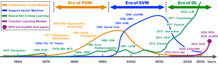
Figure 1: The timeline illustrates the development of various dominant machine learning base models over the past 70 years, with different colors representing different models. Orange Color: probabilistic graphical models (1980s to mid-2000s); Blue Color: support vector machine (mid 1990s to early 2010s); Green Color: deep learning models (mid-2010s to present); and Purple Color: deep function learning (2020s to present).

In this paper, we will introduce a novel deep model, namely Reconciled Polynomial Network (RPN), that can potentially unify these different aforementioned base models into one shared representation. In terms of model architecture, RPN consists of three component functions: data expansion function, parameter reconciliation function and remainder function. Inspired by the Taylor’s theorem, RPN disentangles the input data from model parameters, and approximates the target functions to be inferred as the inner product of the data expansion function with the parameter reconciliation function, subsequently summed with the remainder function.

Based on architecture of RPN, inferring the diverse underlying mapping that governs data distributions (from inputs to outputs) is actually equivalent to inferring these three compositional functions. This inference process of the diverse data distribution mappings based on RPN is named as the function learning task in this paper. Specifically, the “function” term mentioned in the task name refers to not only the mathematical function components composing the RPN model but also the cognitive function of RPN as an intelligent system to relate input signals with desired output response. Function learning has been long-time treated as equivalent to the continuous function fitting and approximation for regression tasks only. Actually, in psychology and cognitive science, researchers have also used the function learning concept for modeling the mental induction process of stimulus-response relations of human and other intelligent subjects [carroll1963functional, koh1991function], involving the acquisition of knowledge, manipulation of information and reasoning. In this paper, we argue that function learning is the most fundamental task in intelligent model learning, encompassing continuous function approximation, discrete vision and language data recognition and prediction, and cognitive and logic dependency relation induction. The following Section 2 will provide an in-depth discussion of function learning and offer a comparative analysis of function learning with the currently prevailing paradigm of representation learning.

Determined by the definitions of the data expansion functions, RPN will project data vectors from the input space to an intermediate (higher-dimensional) space represented with new basis vectors. To address the “curse of dimensionality” issue stemming from the data expansions, the parameter reconciliation function in RPN fabricates a reduced set of parameters into a higher-order parameter matrix. These expanded data vectors are then polynomially integrated via the inner product with these generated reconciled parameters, which further projects these expanded data vectors back to the desired lower-dimensional output space. Moreover, the remainder function provides RPN with additional complementary information to further reduce potential approximation errors. All these component functions within RPN embody concrete physical meanings. These functions, coupled with the straightforward application of simple inner product and summation operators, provide RPN with greater interpretability compared to other existing base models.

RPN possesses a highly versatile architecture capable of constructing models with diverse complexities, capacities, and levels of completeness. In this paper, to provide RPN with greater modeling capabilities in design, we enable RPN to incorporate both a wide architecture featuring multi-heads and multi-channels (within each layer), as well as a deep architecture comprising multi-layers. Additionally, we further offer RPN with a more adaptable and lightweight mechanism for constructing models with comparable capabilities through the nested and extended data expansion functions. These powerful yet flexible design mechanisms provide RPN with greater modeling capability, enabling it to serve as the backbone for unifying various base models mentioned above into a single representation. This includes non-deep models, like probabilistic graphical models (PGMs) - such as Bayesian network [Pearl_CSS85] and Markov network [kindermann1980markov] - and kernel support vector machines (kernel SVMs) [10.1145/130385.130401], as well as deep models like the classic multi-layer perceptron (MLP) [Rumelhart1986LearningRB] and the recent Kolmogorov-Arnold network (KAN) [Liu2024KANKN].

To investigate the effectiveness of RPN for deep function learning tasks, this paper will present extensive empirical experiments conducted on numerous benchmark datasets. Given RPN’s status as a general base model for function learning, we evaluate its performance with datasets in various modalities, including numerical function datasets (for continuous function fitting and approximation), image and text datasets (for discrete vision and language data classification), and classic tabular datasets (for variable dependency relationship inference and induction). The experimental results demonstrate that, RPN outperforms MLP and KAN with mean squared errors at least $\times 10^{-1}$ lower (and even $\times 10^{-2}$ lower in some cases) on continuous function fitting tasks. On both vision and language benchmark datasets, using much less learnable parameters, RPN consistently achieves higher accuracy scores than Naive Bayes, kernel SVM, MLP, and KAN for these discrete data classifications. Moreover, equipped with probabilistic data expansion functions, RPN also learns better probabilistic dependency relationships among variables and outperforms probabilistic models, including Naive Bayes, Bayesian networks, and Markov networks, for learning on the tabular benchmark datasets.

We summarize the contributions of this paper as follows:

• RPN for Deep Function Learning: In this paper, we propose the task of “deep function learning” and introduce a novel deep function learning base model, i.e., the Reconciled Polynomial Network (RPN). RPN has a versatile model architecture and attains superior modeling capabilities for diverse deep function learning tasks on various multi-modality datasets. Moreover, by disentangling input data from model parameters with the expansion, reconciliation and remainder functions, RPN achieves greater interpretability than existing deep and non-deep base models.

• Component Functions: In this paper, we introduce a tripartite set of compositional functions - data expansion, parameter reconciliation, and remainder functions - that serve as the building blocks for the RPN model. By strategically combining these component functions, we can construct a multi-head, multi-channel, and multi-layer architecture, enabling RPN to address a wide spectrum of learning challenges across diverse function learning tasks.

• Base Model Unification: This paper demonstrates that RPN provides a unifying framework for several influential base models, including Bayesian networks, Markov networks, kernel SVMs, MLP, and KAN. We show that, through specific selections of component functions, each of these models can be unified into RPN’s canonical representation, characterized by the inner product of a data expansion function with a parameter reconciliation function, summed with a remainder function.

• Experimental Investigations: This paper presents a series of extensive empirical experiments conducted across numerous benchmark datasets for various deep function learning tasks, including numerical function fitting tasks, discrete image and language data classification tasks, and tabular data based dependency relation inference and induction tasks. The results demonstrate RPN’s consistently superior performance compared to other existing base models, providing strong empirical validations of our proposed model.

• The tinyBIG Toolkit: To facilitate the adoption, implementation and experimentation of RPN, we have released tinyBIG, a comprehensive toolkit for RPN model construction. tinyBIG offers a rich library of pre-implemented functions, including $25$ categories of data expansion functions, $10$ parameter reconciliation functions, and $5$ remainder functions, along with the complete model framework and optimized model training pipelines. This integrated toolkit enables researchers to rapidly design, customize, and deploy RPN models across a wide spectrum of deep function learning tasks.

This paper provides a comprehensive investigation of the proposed Reconciled Polynomial Network model. The remaining parts of this paper will be organized as follows. In Section 2, we will first introduce the novel function learning concept and compare RPN with several existing base models. In Section 3, we will cover notations, task formulations, and essential background knowledge on Taylor’s theorem. In Section 4, we will provide detailed descriptions of RPN model’s architecture and design mechanisms. Our library of expansion, reconciliation, and remainder functions will be presented in Section 5. In Section LABEL:sec:backbone_unification, we demonstrate how RPN unifies and represents existing base models. The experimental evaluation of RPN’s performance on numerous benchmark datasets will be provided in Section LABEL:sec:experiments. After that, we will discuss RPN’s interpretations from both machine learning and biological neuroscience perspectives in Section LABEL:sec:interpretation. In Section LABEL:sec:merits_limitations, we will critically discuss the merits, limitations and potential future works of RPN. Finally, we will introduce the related works in Section LABEL:sec:related_work and conclude this paper in Section LABEL:sec:conclusion.

2 Deep Function Learning

In this section, we will first introduce the concept of deep function learning task. After that, we will provide the detailed clarifications about how deep function learning differs from existing deep representation learning tasks. Based on this concept, we will further compare RPN, the deep function learning model proposed in this paper, with other existing non-deep and deep base models to illustrate their key differences.

2.1 What is Deep Function Learning?

As its name suggests, deep function learning, as the most fundamental task in machine learning, aims to build general deep models composed of a sequence of component functions that infer the relationships between inputs and outputs. These component functions define the mathematical projections across different data and parameter spaces. In deep function learning, without any prior assumptions about the data modalities, the corresponding input and output data can also appear in different forms, including but not limited to continuous numerical values (such as continuous functions), discrete categorical features (such as images and language data), probabilistic variables (defining the dependency relationships between inputs and outputs), and others.

Definition 1

(Deep Function Learning): Formally, given the input and output spaces $\mathbbm{R}^{m}$ and $\mathbbm{R}^{n}$, the underling mapping that governs the data projection between these two spaces can be denoted as:

$$f:\mathbbm{R}^{m}\to\mathbbm{R}^{n}.$$ (1)

Deep function learning aims to build a model $g$ as a composition of deep mathematical function sequences $g_{1},g_{2},\cdots,g_{K}$ to project data cross different vector spaces, which can be represented as

$$g:\mathbbm{R}^{m}\to\mathbbm{R}^{n},\text{ and }g=g_{1}\circ g_{2}\circ\cdots\circ g_{k},$$ (2)

where the $\circ$ notation denotes the component function integration and composition operators. The component functions $g_{i}$ can be defined on either input data or the model parameters.

For input $\mathbf{x}\in\mathbbm{R}^{m}$, if the output generated by the model can approximate the desired output, i.e.,

$$g(\mathbf{x}|\mathbf{w},\boldsymbol{\theta})\approx f(\mathbf{x}),$$ (3)

then model is $g$ can serve as an approximated mapping of $f$. Notations $\mathbf{w}\in\mathbbm{R}^{l}$ and $\boldsymbol{\theta}\in\mathbbm{R}^{l^{\prime}}$ denote the learnable parameters and hyper-parameters of the function learning model, respectively.

Below, we will further clarify the distinctions between deep function learning and current deep model-based data representation learning tasks. After that, we will compare our RPN model, which is grounded in deep function learning, against other existing base models.

2.2 Deep Function Learning vs Deep Representation Learning

As mentioned previously, the function learning tasks and models examined in this paper encompass not only continuous function approximation, but also discrete data classification and the induction of dependency relations. Besides the literal differences indicated by their names - representation learning is data oriented but function learning is model oriented - deep function learning significantly differs from the current deep representation learning in several critical perspectives discussed below.

• Generalizability: Representation learning, to some extent, has contributed to the current fragmentation within the AI community, as data - the carrier of information - is collected, represented, and stored in disparate modalities. Existing deep models, specifically designed for certain modalities, tend to overfit to these modality-specific data representations in addition to learning the underlying information. Applying a model proposed for one modality to another typically necessitates significant architectural redesigns. Recently, there have been efforts to explore the cross-modal applicability of certain models, e.g., CNNs for language and Transformers for vision, but replicating such cross-modality migration explorations across all current and future deep models is extremely expensive and unsustainable. Furthermore, to achieve the future artificial general intelligence (AGI), the available data in a single modality is no longer sufficient for training larger models. Deep function learning, without any prior assumptions on data modalities, will pave the way for improving the model generalizability. These learned functions should demonstrate their generalizability and applicability to multi-modal data from the outset, during their design and investigation phases.

• Interpretability: Representation learning primarily aims to learn and extract latent patterns or salient features from data, aligning with the technological advancements in data science and big data analytics over the past two decades. However, the learned data representations often lack interpretable physical meanings, rendering most current AI models to be black boxes. In contrast, to realize the goal of explainable AI (xAI), greater emphasis must be placed on developing new model architectures with concrete physical meanings and mathematical interpretations in the future. The RPN based deep function learning, on the other hand, aims to learn compositional functions with inherent physical interpretability for building general-purpose models across various tasks, thereby bridging the interpretability gap of current and future deep models.

• Reusability: Representation learning converts input data into embedding vectors that can be stored in vector databases and reused in future applications (e.g., in the retrieval-augmented generation (RAG) models). However, in practical real-world scenarios, the direct usability of such pre-computed embedding representations in vector databases can be quite limited, both in terms of use cases and transactional queries or operations. Moreover, as new data arrives, new architectures are designed, and new model checkpoints are updated in the dynamically evolving online and offline worlds, we may need to re-learn all these embedding representation vectors via fine-tuning or retraining from scratch to maintain consistency, greatly impacting the reusability of representation learning results. In contrast, function learning focuses on learning compositional functions for underlying mapping inference, whose disentangled design is inherently well-suited for reusability and continual learning in future AI systems.

As a special type of machine learning, both deep function learning and deep representation learning are focused on inferring the underlying distributions of data. In contrast to representation learning, deep function learning narrows down the model architecture to a sequence of concrete mathematical functions defined on both data and parameter spaces. The RPN based deep function learning model also disentangles data from parameters and aims to infer and learn these compositional functions, each bearing a concrete physical interpretation for mathematical projections between various data and parameter domains. In contrast, existing deep representation learning models inextricably mix data and parameters together, rendering model interpretability virtually impossible. Below, we will further illustrate the differences of RPN with several existing base models.

2.3 RPN vs Other Base Models

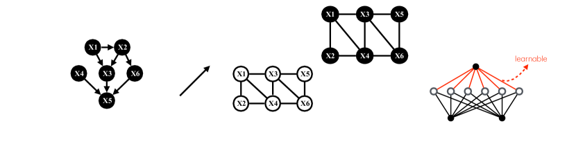
[0.5ex][x]1pt1.5mm

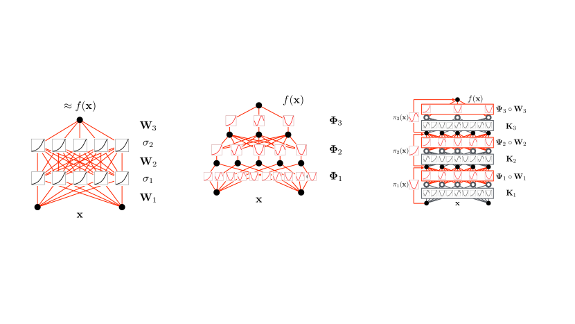
Figure 2: A comparison of RPN with Bayesian Network, Markov Network, Kernel SVM, MLP and KAN in terms of mathematical theorem foundation, formula and model architecture. In the plots, we represent the learnable parameters and functions in the red color, while the unlearnable/fixed ones are represented in the dark/gray colors instead. The inputs and outputs are represented with the solid circles, while the expansions are represented as the hollow circles instead.

Figure 2 compares the RPN model proposed for deep function learning with several base models in terms of mathematical theorem foundations, formula representations, and model architectures. The top three Plots (a)-(c) describe the non-deep base models: Bayesian Networks, Markov Networks, and Kernel SVMs; while the Plots (d)-(i) at the bottom illustrate the architectures of deep base models: MLPs, KANs, and RPN. For MLPs and KANs, Plots (d)-(e) and (g)-(h) illustrate their two-layer and three-layer architectures, respectively. Similarly, for RPN, we present its one-layer and three-layer architectures in Plots (f) and (i).

Based on the plots shown in Figure 2, we can observe significant differences of RPN compared against these base models, which are summarized as follows:

• RPN vs Non-Deep Base Models: Examining the model plots, we observe that all these base model architectures can be represented as graph structures composed of variables and their relationships. The model architecture of the Markov network is undirected, while that of the Bayesian network is directed. Similarly, for MLP, KAN, and RPN, although we haven’t shown the variable connection directions, their model architecture are also directed, flowing from bottom to top. The model architectures of both Markov network and Bayesian network consist of variable nodes that correspond only to input features and output labels. In contrast, for kernel SVM, MLP, KAN, and RPN, their model architectures involve not only nodes representing inputs and outputs, but also those representing expansions and hidden layers. Both RPN and kernel SVM involve a data expansion function to project input data into a high-dimensional space. However, their approaches diverge thereafter. Kernel SVM directly defines parameters within this high-dimensional space to integrate expansion vectors into outputs. In contrast, RPN fabricates these high-dimensional parameters via a reconciliation function from a reduced set of parameters instead.

• RPN vs Deep Base Models: The difference between RPN and MLP is easy to observe. MLP involves neither data expansion nor parameter reconciliation. Instead, they apply activation functions to neurons after input integration, which is parameterized by neuron connection weights. Unlike MLPs with predefined, static activation functions, the recent KAN model proposes to learn the activation functions attached to neuron-neuron connections, with their outputs being directly summed together. RPN, in contrast, integrates the strengths of both kernel SVM and KAN: it employs the expansion function from kernel SVM and adopts learnable functions attached to neuron-to-neuron connections, similar to KANs. Meanwhile, different from kernel SVM, MLP and KAN, RPN introduces a novel approach to fabriate a large number of parameters from a small set. This technique helps address both the “curse of dimension” and the model generalization problems. We have briefly mentioned the “curse of dimension” problem before already, and will discuss about the model generalization issue later in Section LABEL:sec:interpretation from the VC-theory perspective.

Here, we briefly compare these base models with RPN. In the following Section LABEL:sec:backbone_unification, after we introduce the RPN model architecture and the component functions, we will further discuss how to unify these base models into RPN’s canonical representations. More comprehensive information about these base models and other related work will also be provided in Section LABEL:sec:related_work.

3 Notations and Background Knowledge on Taylor’s Theorem

This section first introduces the notation system used throughout this paper. Based on the notations, we then briefly present Taylor’s theorem as the preliminary knowledge of the RPN model, which will be introduced in the following Section 4.

3.1 Notation System

In the sequel of this paper, we will use the lower case letters (e.g., $x$) to represent scalars, lower case bold letters (e.g., $\mathbf{x}$) to denote column vectors, bold-face upper case letters (e.g., $\mathbf{X}$) to denote matrices and high-order tensors, and upper case calligraphic letters (e.g., $\mathcal{X}$) to denote sets. Given a matrix $\mathbf{X}$, we denote $\mathbf{X}(i,:)$ and $\mathbf{X}(:,j)$ as its $i_{th}$ row and $j_{th}$ column, respectively. The ($i_{th}$, $j_{th}$) entry of matrix $\mathbf{X}$ can be denoted as $\mathbf{X}(i,j)$. We use $\mathbf{X}^{\top}$ and $\mathbf{x}^{\top}$ to represent the transpose of matrix $\mathbf{X}$ and vector $\mathbf{x}$. For vector $\mathbf{x}$, we represent its $L_{p}$-norm as $\left\|\mathbf{x}\right\|_{p}=\left(\sum_{i}|\mathbf{x}(i)|^{p}\right)^{\frac{1}{p}}$. The Frobenius-norm of matrix $\mathbf{X}$ is represented as $\left\|\mathbf{X}\right\|_{F}=\left(\sum_{i,j}|\mathbf{X}(i,j)|^{2}\right)^{\frac{1}{2}}$. The elementwise product of vectors $\mathbf{x}$ and $\mathbf{y}$ of the same dimension is represented as $\mathbf{x}\odot\mathbf{y}$, their inner product is represented as $\left\langle\mathbf{x},\mathbf{y}\right\rangle$, and their Kronecker product is $\mathbf{x}\otimes\mathbf{y}$. The elementwise product and Kronecker product operators can also be applied to matrices $\mathbf{X}$ and $\mathbf{Y}$ as $\mathbf{X}\odot\mathbf{Y}$ and $\mathbf{X}\otimes\mathbf{Y}$, respectively.

3.2 Taylor’s Theorem for Univariate Function Approximation

Taylor’s theorem approximates a $d$-times differentiable function around a given point using polynomials up to degree $d$, commonly referred to as the $d_{\text{th}}$-order Taylor polynomial. In this section, we first introduce Taylor’s theorem for univariate functions, which also generalizes to multivariate and vector valued functions. We will briefly describe its extension to multivariate functions in the subsequent Subsection 3.3, and then introduce the RPN model designed based on Taylor’s theorem with vector valued functions in Section 4.

Theorem 1

(Taylor’s Theorem): Let $d\geq 1$ be an integer and let function $f:\mathbbm{R}\to\mathbbm{R}$ be $d$ times differentiable at the point $a\in\mathbbm{R}$. As illustrated in Figure 3, then there exists a function $h_{d}:\mathbbm{R}\to\mathbbm{R}$ such that

$$f(x) =\frac{f(a)}{0!}(x-a)^{0}+\frac{f^{\prime}(a)}{1!}(x-a)^{1}+\frac{f^{\prime\prime}(a)}{2!}(x-a)^{2}+\cdots+\frac{f^{(d)}(a)}{d!}(x-a)^{d}+R_{d}(x),$$ (4)

$$=\sum_{i=0}^{d}\frac{f^{(i)}(a)}{i!}(x-a)^{i}+R_{d}(x).$$

In the equation, $R_{d}(x)$ is also normally called the “remainder” term and can be represented as

$$R_{d}(x)=h_{d}(x)(x-a)^{d}\text{ , where }\lim_{x\to a}h_{d}(x)=0.$$ (5)

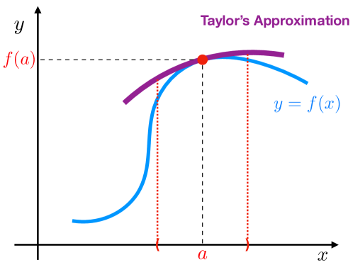
Figure 3: An illustration of Taylor’s approximation of continuous functions.

According to the above description of the Taylor’s Theorem, the function output $f(x)$ can be represent as a summation of polynomials of high degrees of the $(x-a)$. What’s more, in this paper, we propose to further disentangle the variable $x$ from the given constant point $a$. Terms like $(x-a)^{k}$ can be decomposed into summations of polynomials in $x$ alone, with $a$ serving as the coefficients:

$$(x-a)^{d} ={d\choose 0}(-a)^{d-0}x^{0}+{d\choose 1}(-a)^{d-1}x^{1}+\cdots+{d\choose d}(-a)^{d-d}x^{d}.$$ (6)

Based on the decomposition, we can rewrite the above Equation (4) as follows:

$$f(x|a) =\left\langle{\mathbf{x}},\mathbf{c}\right\rangle+R_{d}(x),$$ (7)

where $\left\langle\cdot,\cdot\right\rangle$ denotes the inner product operator. The expanded data vector $\mathbf{x}=\kappa(x)=[x^{0},x^{1},x^{2},\cdots,x^{d}]\in\mathbbm{R}^{d+1}$ contains the high-order polynomials of $x$, where the created coefficient vector $\mathbf{c}=\psi(a)=[c_{0},c_{1},c_{2},\cdots,c_{d}]\in\mathbbm{R}^{d+1}$ has the same dimension as $\mathbf{x}$. Each coefficient term, such as $c_{i}$ (where $i\in\{0,1,\cdots,d\})$, is fabricated with $a$ as follows:

$$c_{i}=\sum_{j=i}^{d}\frac{f^{(j)}(a)}{j!}{j\choose i}(-a)^{j-i}.$$ (8)

The remainder term measure the error in approximating $f$ with Taylor’s polynomials. The representation illustrated in Equation (5) above is known as the “Peano Remainder”. In addition, mathematicians have introduced many different forms of remainder representations, some of which are listed below:

$$\underline{\textbf{(a) Peano Remainder:}}$$ (9)

$$R_{d}(x)=h_{d}(x)(x-a)^{d},$$

$$\text{where }\lim_{x\to a}h_{d}(x)=0.$$

$$\underline{\textbf{(b) Lagrange Remainder:}}$$ (10)

$$R_{d}(x)=\frac{f^{(d+1)}(\xi)}{(d+1)!}{(x-a)^{d+1}},$$

$$\text{for some }\xi\text{ between $a$ and $x$}.$$

$$\underline{\textbf{(c) Cauchy Remainder:}}$$ (11)

$$R_{d}(x)=\frac{f^{(d+1)}(\xi)}{d!}{(x-\xi)^{d}(x-a)},$$

$$\text{for some }\xi\text{ between $a$ and $x$}.$$

$$\underline{\textbf{(d) Schl\"{o}milch Remainder:}}$$ (12)

$$R_{d}(x)=\frac{f^{(d+1)}(\xi)}{d!}{(x-\xi)^{d+1-p}\frac{(x-a)^{p}}{p}},$$

$$\text{for some }p>0\text{ and }\xi\text{ between $a$ and $x$}.$$

3.3 Taylor’s Theorem for Multivariate Function Approximation

Representing multivariate continuous functions with Taylor’s polynomials is more intricate. In this part, we use a multivariate function $f:\mathbbm{R}^{m}\to\mathbbm{R}$ as an example to illustrate how to disentangle the input variables and function parameters via Taylor’s formula. Similar as the above single-variable function, assuming function $f$ is $d_{th}$-time continuously differentiable at point $\mathbf{a}\in\mathbbm{R}^{m}$, then for the inputs near the point can be approximated as

$$f(\mathbf{x})=\sum_{|\alpha|\leq d}\frac{D^{|\alpha|}f(\mathbf{a})}{\alpha!}(\mathbf{x}-\mathbf{a})^{\alpha}+R_{d}(\mathbf{x}).$$ (13)

The notation $D^{|\alpha|}f$ denotes the $|\alpha|_{th}$ partial derivatives of function $f$ and $R_{d}(\mathbf{x})$ denotes the remainder term:

$$\begin{cases}D^{|\alpha|}f&=\frac{\partial^{|\alpha|}f}{\partial x_{1}^{\alpha_{1}}\cdots\partial x_{m}^{\alpha_{m}}}\\ R_{d}(\mathbf{x})&=\sum_{|\alpha|=d}h_{\alpha}(\mathbf{x})(\mathbf{x}-\mathbf{a})^{\alpha}\end{cases},\text{ where }\begin{cases}&|\alpha|\ \ =\alpha_{1}+\alpha_{2}+\cdots+\alpha_{m};\\ &\alpha!\ \ =\alpha_{1}!\alpha_{2}!\cdots\alpha_{m}!;\\ &(\mathbf{x}-\mathbf{a})^{\alpha}\ \ =(x_{1}-a_{1})^{\alpha_{1}}\cdots(x_{m}-a_{m})^{\alpha_{m}};\\ &\lim_{\mathbf{x}\to\mathbf{a}}h_{\alpha}(\mathbf{x})\ \ =0.\end{cases}$$ (14)

Similar to the single-variable case, the variables $\mathbf{x}=[x_{1},x_{2},\cdots,x_{m}]$ involved in the multivariate polynomials can also be decoupled from the data point $\mathbf{a}=[a_{1},a_{2},\cdots,a_{m}]$, leading to the following representation:

$$f(\mathbf{x}|\mathbf{a})=\left\langle\bar{\mathbf{x}},{\mathbf{c}}\right\rangle+R_{d}(\mathbf{x}),$$ (15)

where $\bar{\mathbf{x}}$ denotes the data expansion vector, and $\mathbf{c}$ represents the created coefficient vector. Their detailed representations are provided as follows.

• Data Expansion: Function $\kappa:\mathbbm{R}^{m}\to\mathbbm{R}^{D}$ will expand the input vector $\mathbf{x}=[x_{1},x_{2},\cdots,x_{m}]^{\top}$ to $\bar{\mathbf{x}}\in\mathbbm{R}^{D}$ as follows:

  $$\bar{\mathbf{x}}=\kappa(\mathbf{x})=[\underbrace{1}_{\text{1 term of order 0}},\underbrace{x_{1},x_{2},\cdots,{x_{m}}}_{\text{$m$ terms of order 1}},\underbrace{x_{1}^{2},x_{1}x_{2},\cdots,{x_{m}^{2}}}_{\text{$m^{2}$ terms of order 2}},\underbrace{\cdots}_{\cdots},\underbrace{\cdots,x_{m}^{d}}_{\text{$m^{d}$ terms of order $d$}}]^{\top},$$ (16)

  where the expansion output vector has a dimension of $D=\sum_{i=0}^{d}m^{i}$.

• Parameter Fabrication: Function $\psi:\mathbbm{R}^{m}\to\mathbbm{R}^{D}$ will fabricate the constant $\mathbf{a}$ to a coefficient vector of dimension $D$ as follows:

  $${\mathbf{c}}=\psi(\mathbf{a})=[\underbrace{c_{0}}_{\text{coeff. of constant}},\underbrace{c_{1},c_{2},\cdots,c_{m}}_{\text{coeff. of terms with order 1}},\underbrace{c_{1,1},c_{1,2},\cdots,c_{m,m}}_{\text{coeff. of terms with order 2}},\underbrace{\cdots}_{\cdots},\underbrace{\cdots,c_{m,m,\cdots,m}}_{\text{coeff. of terms with order d}}]^{\top}.$$ (17)

  The coefficient vector $\mathbf{c}$ has the same dimension as $\bar{\mathbf{x}}$, and the coefficient $c_{i_{1},i_{2},\cdots,i_{k}}$ corresponds to the polynomial term $x_{i_{1}}x_{i_{2}}\cdots x_{i_{k}}$. As to the specific representation of $c_{i_{1},i_{2},\cdots,i_{k}}$, it can be obtained by decomposing the above Equations (13)-(14).

• Lagrange Remainder: The remainder $R_{d}(\mathbf{x})$ will include all the terms with order higher than $d$, which can reduce the approximation errors.

3.4 Taylor’s Theorem based Machine Learning Models

In real-world problems, the underlying functional mappings are often more intricate, such as $f:\mathbbm{R}^{m}\to\mathbbm{R}^{n}$ with multiple input variables and multiple outputs. Representing these functions with Taylor’s polynomials requires more cumbersome derivations, and the coefficient fabrication outputs should be a two-dimensional matrix, such as $\psi(\mathbf{a})\in\mathbbm{R}^{n\times D}$. To avoid getting bogged down in unnecessary mathematical details, we will not repeat those derivations here.

In recent years, there has been a growing interest in designing machine learning and deep learning models based on Taylor’s theorem. For binary data inputs, Zhang et al. [Zhang2018ReconciledPM] introduce the reconciled polynomial machine to unify shallow and deep learning models, which is also the prior work that this paper is based on. Balduzzi et al. [Balduzzi2016NeuralTA] investigate the convergence and exploration in rectifier networks with neural Taylor approximations, while Chrysos et al. [Chrysos2020DeepPN] propose a new class of function approximation method based on polynomial expansions. Zhao et al. [zhao2023taylornet] propose a generic neural architecture TaylorNet based on tensor decomposition to initialize the models, and Nivron et al. [Nivron2023TaylorformerPP] introduce to incorporate use Taylor’s expansion as a wrapper of transformer for the probabilistic predictions for time series and other random processes. Beyond time series and continuous function approximation, Taylor’s expansion has found applications in reinforcement learning and computer vision. [Tang2020TaylorEP] investigates the application of Taylor’s expansions in reinforcement learning and introduces the Taylor expansion policy optimization to generalize prior work; and [Pfrommer2022TaSILTS] introduces a simple augmentation to standard behavior cloning losses in the context of continuous control for Taylor series imitation learning. In image processing, [Zhou2021UnfoldingTA] proposes to use Taylor’s formula to construct a novel framework for image restoration, and [10070581] proposes the Taylor neural net for image super-resolution.

Different these prior work, since the underlying function $f$ is unknown, we cannot directly employ the above derivations and Taylor’s expansions to define approximated polynomial representations of $f$ for practical applications. Drawing inspiration from the approximation architecture delineated in Equation 7 and Equation 15, we propose a novel approach that defines distinct component functions to substitute the data vector, coefficient vector, and remainder terms. Additionally, as the input variable $\mathbf{x}$ varies across instances, instead of manually selecting one single fixed constant $\mathbf{a}$, we propose to define it as multi-channel parameters and learn them instead. These innovations form the foundation of our proposed Reconciled Polynomial Network (our) model to be introduced in the following section.

4 RPN: Reconciled Polynomial Network for Deep Function Learning

Based on the preliminary background introduced above and inspired by the work of [Zhang2018ReconciledPM], we will introduce the Reconciled Polynomial Network (RPN) model for function learning in this section.

4.1 RPN: Reconciled Polynomial Network

Formally, given the underlying data distribution mapping $f:\mathbbm{R}^{m}\to\mathbbm{R}^{n}$, we represent the RPN model proposed to approximate function $f$ as follows:

$${g(\mathbf{x}|\mathbf{w})=\left\langle\kappa(\mathbf{x}),\psi(\mathbf{w})\right\rangle+\pi(\mathbf{x}),}$$ (18)

where

• $\kappa:\mathbbm{R}^{m}\to\mathbbm{R}^{D}$ is named as the data expansion function and $D$ is the target expansion space dimension.

• $\psi:\mathbbm{R}^{l}\to\mathbbm{R}^{n\times D}$ is named as the parameter reconciliation function, which is defined only on the parameters without any input data.

• $\pi:\mathbbm{R}^{m}\to\mathbbm{R}^{n}$ is named as the remainder function.

The architecture of RPN is also illustrated in Figure 4. The RPN model disentangles input data from model parameters through the expansion functions $\kappa$ and reconciliation function $\psi$. More detailed information about all these components and modules mentioned in Figure 4 will be introduced in the following parts of this section.

4.2 RPN Component Functions

The data expansion function $\kappa$ projects input data into a new space with different basis vectors, where the target vector space dimension $D$ is determined when defining $\kappa$. In practice, the function $\kappa$ can either expand or compress the input to a higher- or lower-dimensional space. The corresponding function, $\kappa$, can also be referred to as the data expansion function (if $D>m$) and data compression function (if $D<m$), respectively. Collectively, these can be unified under the term “data transformation functions”. In this paper, we focus on expanding the inputs to a higher-dimensional space, and will use the function names “data transformation” and “data expansion” interchangeably in the following sections.

Meanwhile, the parameter reconciliation function $\psi$ adjusts the available parameter vector of length $l$ by fabricating a new parameter matrix of size $n\times D$ to accommodate the expansion space dimension $D$ defined by function $\kappa$. In most of the cases studied in this paper, the parameter vector length $l$ is much smaller than the output matrix size $n\times D$, i.e., $l\ll n\times D$. Meanwhile, in practice, we can also define function $\psi$ to fabricate a longer parameter vector into a smaller parameter matrix, i.e., $l>n\times D$. To unify these different cases, the data reconciliation function can also be referred to as the “parameter fabrication function”, and these function names will be used interchangeably in this paper.

Without specific descriptions, the remainder function $\pi$ defined here is based solely on the input data $\mathbf{x}$. However, in practice, we also allow $\pi$ to include learnable parameters for output dimension adjustment. In such cases, it should be rewritten as $\pi(\mathbf{x}|\mathbf{w}^{\prime})$, where $\mathbf{w}^{\prime}$ is one extra fraction of the model’s learnable parameters. Together with the parameter vector $\mathbf{w}$ (i.e., the input to the parameter reconciliation function $\psi$), they will define the complete set of learnable parameters for the model.

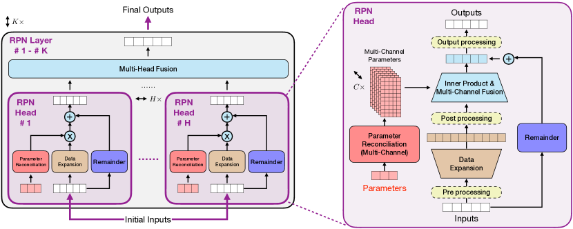
Figure 4: An illustration of the RPN framework. The left plot illustrates the multi-layer ($K$-layer) architecture of RPN. Each layer involves multi-head for function learning, whose outputs will be fused together. The right plot illustrates the detailed architecture of the RPN head, involving data expansion, multi-channel parameter reconciliation, remainder, and their internal operations. The components with yellow color in dashed lines denote the optional data processing functions (e.g., activation functions and norm functions) for the inputs, expansions and outputs.

4.3 Wide RPN: Multi-Head and Multi-Channel Model Architecture

Similar to the Transformer with multi-head attention [Vaswani2017AttentionIA], as shown in Figure 4, the RPN model employs a multi-head architecture, where each head can disentangle the input data and model parameters using different expansion, reconciliation and remainder functions, respectively:

$$g(\mathbf{x}|\mathbf{w},H)=\sum_{h=0}^{H-1}\left\langle\kappa^{(h)}(\mathbf{x}),\psi^{(h)}(\mathbf{w}^{(h)})\right\rangle+\pi^{(h)}(\mathbf{x}),$$ (19)

where the superscript “$h$” indicates the head index and $H$ denotes the total head number. By default, we use summation to combine the results from all these heads.

Moreover, in the RPN model shown in Figure 4, similar to convolutional neural networks (CNNs) employing multiple filters, we allow each head to have multiple channels of parameters applied to the same data expansion. For example, for the $h_{th}$ head, we define its multi-channel parameters as $\mathbf{w}^{(h),0},\mathbf{w}^{(h),1},\cdots,\mathbf{w}^{(h),C-1}$, where $C$ denotes the number of channels. These parameters will be reconciled using the same parameter reconciliation function, as shown below:

$$g(\mathbf{x}|\mathbf{w},H,C)=\sum_{h=0}^{H-1}\sum_{c=0}^{C-1}\left\langle\kappa^{(h)}(\mathbf{x}),\psi^{(h)}(\mathbf{w}^{(h),c})\right\rangle+\pi^{(h)}(\mathbf{x}),$$ (20)

The multi-head, multi-channel design of the RPN model allows it to project the same input data into multiple different high-dimensional spaces simultaneously. Each head and channel combination may potentially learn unique features from the data. The unique parameters at different heads can have different initialized lengths, and each of them will be processed in unique ways to accommodate the expanded data. This multi-channel approach provides our model with more flexibility in model design. In the following parts of this paper, to simplify the notations, we will illustrate the model’s functional components using a single-head, single-channel architecture by default. However, readers should note that these components to be introduced below can be extended to their multi-head, multi-channel designs in practical implementations.

4.4 Deep RPN: Multi-Layer Model Architecture

The wide model architecture introduced above provides RPN with greater capabilities for approximating functions with diverse expansions concurrently. However, such shallow architectures can be insufficient for modeling complex functions. In this paper, as illustrated in Figure 4, we propose to stack RPN layers on top of each other to build a deeper architecture, where the Equation (18) actually defines one single layer of the model. Formally, we can represent the deep RPN with multi-layers as follows:

$$\begin{cases}\text{Input: }&\mathbf{h}_{0}=\mathbf{x},\\ \text{Layer 1: }&\mathbf{h}_{1}=\left\langle\kappa_{1}(\mathbf{h}_{0}),\psi_{1}(\mathbf{w}_{1})\right\rangle+\pi_{1}(\mathbf{h}_{0}),\\ \text{Layer 2: }&\mathbf{h}_{2}=\left\langle\kappa_{2}(\mathbf{h}_{1}),\psi_{2}(\mathbf{w}_{2})\right\rangle+\pi_{2}(\mathbf{h}_{1}),\\ \cdots&\cdots\ \cdots\\ \text{Layer K: }&\mathbf{h}_{K}=\left\langle\kappa_{K}(\mathbf{h}_{K-1}),\psi_{K}(\mathbf{w}_{K})\right\rangle+\pi_{K}(\mathbf{h}_{K-1}),\\ \text{Output: }&\hat{\mathbf{y}}=\mathbf{h}_{K}.\end{cases}$$ (21)

The subscripts used above denote the layer index. The dimensions of the outputs at each layer can be represented as a list $[d_{0},d_{1},\cdots,d_{K-1},d_{K}]$, where $d_{0}=m$ and $d_{K}=n$ denote the input and the desired output dimensions, respectively. Therefore, if the component functions at each layer of our model have been predetermined, we can just use the dimension list $[d_{0},d_{1},\cdots,d_{K-1},d_{K}]$ to represent the architecture of the RPN model.

4.5 Versatile RPN: Nested and Extended Expansion Functions

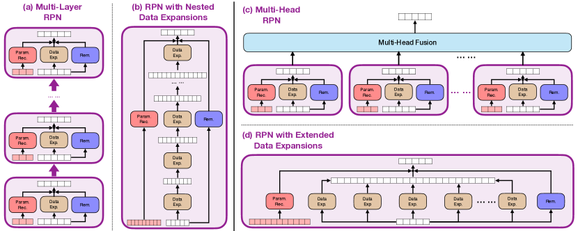
Figure 5: An illustration of the RPN layer with nested and extended data expansions. Plot (a): multi-layer RPN; Plot (b): single-layer RPN with nested data expansions; Plot (c): multi-head RPN; Plot (d): single-head RPN with extended data expansions.

The data expansion function introduced earlier projects the input data to a higher-dimensional space. There exist different ways to define the data expansion function, and a list of such basic expansion functions will be introduced in the following Section 5.1. The multi-head, multi-channel and multi-layer architecture also provides RPN with more capacity to build wider and deeper architectures for projecting input data to the desired target space. In addition to these designs, as illustrated in Figure 5, RPN also provides a more flexible and lightweight mechanism to build models with similar capacities via the nested and extended data expansion functions.

Nested expansions: Formally, given a list of $n$ data expansion functions $\kappa_{1}:\mathbbm{R}^{d_{0}}\to\mathbbm{R}^{d_{1}}$, $\kappa_{2}:\mathbbm{R}^{d_{1}}\to\mathbbm{R}^{d_{2}}$, $\cdots$, $\kappa_{n}:\mathbbm{R}^{d_{n-1}}\to\mathbbm{R}^{d_{n}}$, as shown in Plots (a)-(b) of Figure 5, the nested calls of these functions will project a data vector from the input space $\mathbbm{R}^{d_{0}}$ to the desired output space $\mathbbm{R}^{d_{n}}$, defining the nested data expansion function $\kappa:\mathbbm{R}^{m}\to\mathbbm{R}^{D}$ as follows:

$$\kappa(\mathbf{x})=\kappa_{n}\left(\kappa_{n-1}\left(\cdots\kappa_{2}\left(\kappa_{1}\left(\mathbf{x}\right)\right)\right)\right)\in\mathbbm{R}^{D}.$$ (22)

where the function input and output dimensions should be $d_{0}=m$ and $d_{n}=D$.

Extended expansions: In addition to nesting these $n$ expansion functions, as shown in Plots (c)-(d) of Figure 5, they can also be concatenated and applied concurrently, with their extended outputs allowing the model to leverage multiple expansion functions simultaneously. Formally, we can represent the extended data expansion function $\kappa:\mathbbm{R}^{m}\to\mathbbm{R}^{D}$ defined based on $\kappa_{1}:\mathbbm{R}^{m}\to\mathbbm{R}^{d_{1}}$, $\kappa_{2}:\mathbbm{R}^{m}\to\mathbbm{R}^{d_{2}}$, $\cdots$, $\kappa_{n}:\mathbbm{R}^{m}\to\mathbbm{R}^{d_{n}}$ as follows:

$$\kappa(\mathbf{x})=\left[\kappa_{1}\left(\mathbf{x}\right),\kappa_{2}\left(\mathbf{x}\right),\cdots,\kappa_{n}\left(\mathbf{x}\right)\right]\in\mathbbm{R}^{D},$$ (23)

where the extended expansion’s output dimension is equal to the sum of the output dimensions from all the individual expansion functions, i.e., $D=\sum_{i=1}^{n}d_{i}$.

As illustrated in Figure 5, the nested expansion functions can define complex expansions akin to the multi-layer architecture of RPN mentioned above. Meanwhile, the extended expansion functions can define expansions similar to the multi-head architecture of RPN. Both nested and extended expansions allow for faster data expansions, circumventing cumbersome parameter inference and remainder function calculation, and can reduce the additional learning costs associated with training deep and wide architectures of our model. This flexibility afforded by nested and extended expansions provides us with greater versatility in designing the RPN model.

4.6 Learning Correctness of RPN: Complexity, Capacity and Completeness

The learning correctness of RPN is fundamentally determined by the compositions of its component functions, each contributing from different perspectives:

• Model Complexity: The data expansion function $\kappa$ expands the input data by projecting its representations using basis vectors in the new space. In other words, function $\kappa$ determines the upper bound of the RPN model’s complexity.

• Model Capacity: The reconciliation function $\psi$ processes the parameters to match the dimensions of the expanded data vectors. The reconciliation function and parameters jointly determine the learning capacity and associated training costs of the RPN model.

• Model Completeness: The remainder function $\pi$ completes the approximation as a residual term, governing the learning completeness of the RPN model.

In the following Section 5, we will introduce several different representations for the data expansion function $\kappa$, parameter reconciliation function $\psi$, and remainder function $\pi$. By strategically combining these component functions, we can construct a multi-head, multi-channel, and multi-layer architecture, enabling RPN to address a wide spectrum of learning challenges across diverse learning tasks.

4.7 Learning Cost of RPN: Space, Time and Parameter Number

To analyze the learning costs of RPN, we can take a batch input $\mathbf{X}\in\mathbbm{R}^{B\times m}$ of batch size $B$ as an example, which will be fed to the RPN model with $K$ layers, each with $H$ heads and each head has $C$ channels. Each head will project the data instance from a vector of length $m$ to an expanded vector of length $D$ and then further projected to the desired output of length $n$. Each channel reconciles parameters from length $l$ to the sizes determined by both the expansion space and output space dimensions, i.e., $n\times D$.

Based on the above hyper-parameters, assuming the input and output dimensions at each layer are comparable to $m$ and $n$, then the space, time costs and the number of involved parameters in learning the RPN model are calculated as follows:

• Space Cost: The total space cost for data (including the inputs, expansions and outputs) and parameter (including raw parameters, fabricated parameters generated by the reconciliation function and optional remainder function parameters) can be represented as $\mathcal{O}(KH(\underbrace{B(\underbrace{m}_{\text{input}}+\underbrace{D}_{\text{expansion}}+\underbrace{n}_{\text{output}})}_{\text{space cost for data}}+\underbrace{C(\underbrace{l}_{\text{raw param.}}+\underbrace{nD}_{\text{reconciled param.}})+\underbrace{mn}_{\text{(optional) remainder param.}}}_{\text{space cost for parameters}}))$.

• Time Cost: Depending on the expansion and reconciliation functions used for building RPN, the total time cost of RPN can be represented as $\mathcal{O}(KH(\underbrace{t_{exp}(m,D)}_{\text{time cost for data exp.}}+\underbrace{Ct_{rec}(l,D)}_{\text{time cost for param. rec.}}+\underbrace{CmnD}_{\text{time cost for inner product}}+\underbrace{mn}_{\text{(optional) time cost for remainder}}))$, where notations $t_{exp}(m,D)$ and $t_{rec}(l,D)$ denote the expected time costs for data expansion and parameter reconciliation functions, respectively.

• Learnable parameters: The total number of parameters in RPN will be $\mathcal{O}(KHCl+KHmn)$, where $\mathcal{O}(KHmn)$ denotes the optional parameter number used for defining the remainder function.

for tree= forked edges, grow’=0, s sep=2.1pt, draw, rounded corners, node options=align=center,, text width=2.7cm, , [Reconciled
Polynomial
Network
(RPN), fill=Plum!30, parent [Data
Expansion
Functions, for tree=fill=brown!45, child [1. Identity Expansion, fill=brown!30, grandchild [1-(a). $\kappa(\mathbf{x})=\mathbf{x}$, fill=brown!30, greatgrandchild [dim: $D=m$, fill=brown!15, referenceblock] ] [1-(b). $\kappa(\mathbf{x})=\sigma(\mathbf{x})$, fill=brown!30, greatgrandchild [dim: $D=m$, fill=brown!15, referenceblock] ] ] [2. Reciprocal Expansion, fill=brown!30, grandchild [2-(a). $\kappa(\mathbf{x})=\frac{{1}}{\mathbf{x}}$, fill=brown!30, greatgrandchild [dim: $D=m$, fill=brown!15, referenceblock] ] [2-(b). $\kappa(\mathbf{x})=\sigma\left(\frac{{1}}{\mathbf{x}}\right)$, fill=brown!30, greatgrandchild [dim: $D=m$, fill=brown!15, referenceblock] ] ] [3. Linear Expansion, fill=brown!30, grandchild [3-(a). $\kappa(\mathbf{x})=c\mathbf{x}$, fill=brown!30, greatgrandchild [dim: $D=m$, fill=brown!15, referenceblock] ] [3-(b). $\kappa(\mathbf{x})=\mathbf{x}\mathbf{C}_{post}$, fill=brown!30, greatgrandchild [dim: $D=m$, fill=brown!15, referenceblock] ] [3-(c). $\kappa(\mathbf{x})=\mathbf{C}_{pre}\mathbf{x}^{\top}$, fill=brown!30, greatgrandchild [dim: $D=m$, fill=brown!15, referenceblock] ] ] [4. Taylor Expansion, fill=brown!30, grandchild [4-(a). $\kappa(\mathbf{x}|d)=[P_{1}(\mathbf{x}),P_{2}(\mathbf{x}),\cdots,P_{d}(\mathbf{x})]$, fill=brown!30, greatgrandchild [dim: $D=\sum_{i=1}^{d}m^{i}$, fill=brown!15, referenceblock] ] ] [5. Fourier Expansion, fill=brown!30, grandchild [5-(a). $\kappa(\mathbf{x}|P,N)$ = $[\cos(2\pi\frac{i}{P}\mathbf{x}),\sin(2\pi\frac{i}{P}\mathbf{x})]_{i=1}^{N}$, fill=brown!30, greatgrandchild [dim: $D=2mN$, fill=brown!15, referenceblock] ] ] [6. B-Spline Expansion, fill=brown!30, grandchild [6-(a). $\kappa(\mathbf{x}|t,d)=[B_{0,d-1}(\mathbf{x}),\cdots,B_{t-1,d-1}(\mathbf{x})]$, fill=brown!30, greatgrandchild [dim: $D=m(t+d)$, fill=brown!15, referenceblock] ] ] [7. Chebyshev Expansion, fill=brown!30, grandchild [7-(a). $\kappa(\mathbf{x}|d)=[T_{1}(\mathbf{x}),T_{2}(\mathbf{x})\cdots,T_{n}(\mathbf{x})]$, fill=brown!30, greatgrandchild [dim: $D=md$, fill=brown!15, referenceblock] ] ] [8. Jacobi Expansion, fill=brown!30, grandchild [8-(a). $\kappa(\mathbf{x}|d)=\left[P_{1}^{(\alpha,\beta)}(\mathbf{x}),P_{2}^{(\alpha,\beta)}(\mathbf{x}),\cdots,P_{d}^{(\alpha,\beta)}(\mathbf{x})\right]$, fill=brown!30, greatgrandchild [dim: $D=md$, fill=brown!15, referenceblock] ] ] [9. Trigonometric Expansion, fill=brown!30, grandchild [9-(a). $\kappa(\mathbf{x})=[\cos(\mathbf{x}),\sin(\mathbf{x}),\tan(\mathbf{x})]$, fill=brown!30, greatgrandchild [dim: $D=3m$, fill=brown!15, referenceblock] ] [9-(b). $\kappa(\mathbf{x})=[\arccos(\mathbf{x}),\arcsin(\mathbf{x}),\arctan(\mathbf{x})]$, fill=brown!30, greatgrandchild [dim: $D=3m$, fill=brown!15, referenceblock] ] ] [10. Hyperbolic Expansion, fill=brown!30, grandchild [10-(a). $\kappa(\mathbf{x})=[\cosh(\mathbf{x}),\sinh(\mathbf{x}),\tanh(\mathbf{x})]$, fill=brown!30, greatgrandchild [dim: $D=3m$, fill=brown!15, referenceblock] ] [10-(b). $\kappa(\mathbf{x})=[\text{arccosh}(\mathbf{x}),\text{arcsinh}(\mathbf{x}),\text{arctanh}(\mathbf{x})]$, fill=brown!30, greatgrandchild [dim: $D=3m$, fill=brown!15, referenceblock] ] ] [11. RBF Expansion, fill=brown!30, grandchild [11-(a). $\kappa(\mathbf{x}|d)=\left[\varphi(\mathbf{x}|c_{1}),\varphi(\mathbf{x}|c_{2}),\cdots,\varphi(\mathbf{x}|c_{d})\right]$, fill=brown!30, greatgrandchild [dim: $D=md$, fill=brown!15, referenceblock] ] ] [12. Combinatorial Expansion, fill=brown!30, grandchild [12-(a). $\kappa(\mathbf{x})=\left[{\mathbf{x}\choose 1},{\mathbf{x}\choose 2},\cdots,{\mathbf{x}\choose d}\right]$, fill=brown!30, greatgrandchild [dim: $D=\sum_{i=1}^{d}i\cdot{m\choose i}$, fill=brown!15, referenceblock] ] ] [13. Probabilistic Expansion, fill=brown!30, grandchild [13-(a). $\kappa(\mathbf{x}|d,\boldsymbol{\theta})=\left[\log P\left({\mathbf{x}}|\theta_{1}\right),\cdots,\log P\left({\mathbf{x}}|\theta_{d}\right)\right]$, fill=brown!30, greatgrandchild [dim: $D=md$, fill=brown!15, referenceblock] ] [13-(b). $\kappa(\mathbf{x}|d,\boldsymbol{\theta})$ = $\left[\log P\left({\mathbf{x}\choose 1}|\theta_{1}\right),\cdots,\log P\left({\mathbf{x}\choose d}|\theta_{d}\right)\right]$, fill=brown!30, greatgrandchild [dim: $D=\sum_{i=1}^{d}{m\choose i}$, fill=brown!15, referenceblock] ] ] ] [Parameter Reconciliation
Functions, for tree=fill=red!45,child [1. Constant Reconciliation, fill=red!30, grandchild [1-(a). $\psi(\mathbf{w})=\mathbf{c}$, fill=red!20, greatgrandchild [$l=0$, fill=red!10, referenceblock] ] [1-(b). $\psi(\mathbf{w})=\mathbf{0}$, fill=red!20, greatgrandchild [$l=0$, fill=red!10, referenceblock] ] [1-(c). $\psi(\mathbf{w})=\mathbf{I}$, fill=red!20, greatgrandchild [$l=0$, fill=red!10, referenceblock] ] ] [2. Identity Reconciliation, fill=red!30, grandchild [2-(a). $\psi(\mathbf{w})=\mathbf{w}$, fill=red!20, greatgrandchild [$l=nD$, fill=red!10, referenceblock] ] ] [3. Masking Reconciliation, fill=red!30, grandchild [3-(a). $\psi({\mathbf{w}}|p)=\mathbf{M}\odot\mathbf{W}$, fill=red!20, greatgrandchild [$l=p\cdot nD$, fill=red!10, referenceblock] ] ] [4. Duplicated Padding Rec., fill=red!30, grandchild [4-(a). $\psi(\mathbf{w}|p)=\mathbf{C}\otimes\mathbf{W}$, fill=red!20, greatgrandchild [$l=\frac{nD}{pq}$, fill=red!10, referenceblock] ] ] [5. Low-Rank Reconciliation, fill=red!30, grandchild [5-(a). $\psi(\mathbf{w})=\mathbf{A}\mathbf{B}^{\top}$, fill=red!20, greatgrandchild [$l=nr+Dr$, fill=red!10, referenceblock] ] ] [6. HM Reconciliation, fill=red!30, grandchild [6-(a). $\psi(\mathbf{w}|p)=\mathbf{A}\otimes\mathbf{B}$, fill=red!20, greatgrandchild [$l=pq+\frac{nD}{pq}$, fill=red!10, referenceblock] ] ] [7. LPHM Reconciliation, fill=red!30, grandchild [7-(a). $\psi(\mathbf{w}|p)=\mathbf{A}\otimes\mathbf{B}=\mathbf{A}\otimes(\mathbf{C}\mathbf{D}^{\top})$, fill=red!20, greatgrandchild [$l=pq+r(\frac{n}{p}+\frac{D}{q})$, fill=red!10, referenceblock] ] ] [8. Dual LPHM Reconciliation, fill=red!30, grandchild [8-(a). $\psi(\mathbf{w}|p)=\mathbf{A}\otimes\mathbf{B}=(\mathbf{P}\mathbf{Q}^{\top})\otimes(\mathbf{C}\mathbf{D}^{\top})$, fill=red!20, greatgrandchild [$l=r(p+q+\frac{n}{p}+\frac{D}{q})$, fill=red!10, referenceblock] ] ] [9. HyperNet Reconciliation, fill=red!30, grandchild [9-(a). $\psi(\mathbf{w})=\text{HyperNet}(\mathbf{w})$, fill=red!20, greatgrandchild [dim: $l$ manual setup, fill=red!10, referenceblock] ] ] ] [Remainder Functions, for tree=fill=blue!45, child [1. Constant Remainder, fill=blue!30, grandchild [1-(a). $\pi(\mathbf{x})=\mathbf{c}$, fill=blue!20, greatgrandchild [no parameter, fill=blue!10, referenceblock] ] [1-(b). $\pi(\mathbf{x})=\mathbf{0}$ (zero remainder), fill=blue!20, greatgrandchild [no parameter, fill=blue!10, referenceblock] ] ] [2. Identity Remainder, fill=blue!30, grandchild [2-(a). $\pi(\mathbf{x})=\mathbf{x}$, fill=blue!20, greatgrandchild [requires parameter, fill=blue!10, referenceblock] ] [2-(b). $\pi(\mathbf{x})=\sigma(\mathbf{x})$, fill=blue!20, greatgrandchild [requires parameter, fill=blue!10, referenceblock] ] ] [3. Linear Remainder, fill=blue!30, grandchild [3-(a). $\pi(\mathbf{x})=\mathbf{x}\mathbf{W}^{\prime}$, fill=blue!20, greatgrandchild [requires parameter, fill=blue!10, referenceblock] ] [3-(b). $\pi(\mathbf{x})=\sigma(\mathbf{x}\mathbf{W}^{\prime})$, fill=blue!20, greatgrandchild [requires parameter, fill=blue!10, referenceblock] ] ] [4. Expansion Remainder, fill=blue!30, grandchild [4-(a). $\pi(\mathbf{x}|\mathbf{w}^{\prime})=\left\langle\kappa^{\prime}(\mathbf{x}),\psi^{\prime}(\mathbf{w}^{\prime})\right\rangle+\pi^{\prime}(\mathbf{x})$, fill=blue!20, greatgrandchild [requires parameter, fill=blue!10, referenceblock] ] ] ] ]

Figure 6: An overview of data expansion, parameter reconciliation, and remainder functions implemented in the tinyBIG toolkit for constructing the RPN model architecture.

5 List of Expansion, Reconciliation and Remainder Functions for RPN Model

This section introduces the expansion, reconciliation, and remainder functions that can be used to design the RPN model, all of which have been implemented in the tinyBIG toolkit and are readily available. Readers seeking a concise overview can refer to Figure 6, which summarizes the lists of expansion, reconciliation and remainder functions to be introduced in this section.

5.1 Data Expansion Functions

The data expansion function determines the complexity of RPN. We will introduce several different data expansion functions below. In real-world practice, these individual data expansions introduced below can also be nested and extended to define more complex expansions, which provides more flexibility in the design of our RPN model.

5.1.1 Identity and Reciprocal Data Expansion

The simplest data expansion methods are the identity data expansion and reciprocal data expansion, which project the input data vector $\mathbf{x}\in\mathbbm{R}^{m}$ onto itself and its reciprocal, potentially with minor transformations via some activation functions, as denoted below:

$$\kappa(\mathbf{x})=\mathbf{x}\in\mathbbm{R}^{D}\text{, and }\kappa(\mathbf{x})=\frac{{1}}{\mathbf{x}}\in\mathbbm{R}^{D},$$ (24)

or

$$\kappa(\mathbf{x})=\sigma(\mathbf{x})\in\mathbbm{R}^{D}\text{, and }\kappa(\mathbf{x})=\sigma\left(\frac{{1}}{\mathbf{x}}\right)\in\mathbbm{R}^{D}.$$ (25)

In the above equations, $\sigma$ denotes an optional activation function (e.g., sigmoid, ReLU, SiLU) or normalization function (e.g., layer-norm, batch-norm, instance-norm). For both the identity and reciprocal expansion functions, their output dimension is equal to the input dimension, i.e., $D=m$.

For all the other expansion functions introduced hereafter, as mentioned in the previous Figure 4, we can also apply the (optional) activation and normalization functions both before and after the expansion by default.

5.1.2 Linear Data Expansion

In certain cases, we may need to adjust the value scales of $\mathbf{x}$ linearly without altering the basis vectors or the dimensions of the space. This can be accomplished through the linear data expansion function. Formally, the linear data expansion function projects the input data vector $\mathbf{x}\in\mathbbm{R}^{m}$ onto itself via linear projection, as follows:

$$\kappa(\mathbf{x})=c\mathbf{x}\in\mathbbm{R}^{D},$$ (26)

or

$$\kappa(\mathbf{x})=\mathbf{x}\mathbf{C}_{post}\in\mathbbm{R}^{D},$$ (27)

or

$$\kappa(\mathbf{x})=\mathbf{C}_{pre}\mathbf{x}^{\top}\in\mathbbm{R}^{D},$$ (28)

where the activation function or norm function $\sigma$ is optional, and $c\in\mathbbm{R}$, $\mathbf{C}_{post},\mathbf{C}_{pre}\in\mathbbm{R}^{m\times m}$ denote the provided constant scalar and linear transformation matrices, respectively. Linear data expansion will not change the data vector dimensions, and the output data vector dimension $D=m$.

5.1.3 Taylor’s Polynomials based Data Expansions

Given a vector $\mathbf{x}=[x_{1},x_{2},\cdots,x_{m}]\in\mathbbm{R}^{m}$ of dimension $m$, the multivariate composition of order $d$ defined based on $\mathbf{x}$ can be represented as a list of potential polynomials composed by the product of the vector elements $x_{1}$, $x_{2}$, $\cdots$, $x_{m}$, where the sum of the degrees equals $d$, i.e.,

$$P_{d}(\mathbf{x})=[x_{1}^{d_{1}}x_{2}^{d_{2}}\cdots x_{m}^{d_{m}}]_{d_{1},d_{2},\cdots,d_{m}\in\{0,1,\cdots m\}\land\sum_{i=1}^{m}d_{i}=d}.$$ (29)

Some examples of the multivariate polynomials are provided as follows:

$$P_{0}(\mathbf{x}) =[1]\in\mathbbm{R}^{1},$$ (30)

$$P_{1}(\mathbf{x}) =[x_{1},x_{2},\cdots,x_{m}]\in\mathbbm{R}^{m},$$

$$P_{2}(\mathbf{x}) =[x_{1}^{2},x_{1}x_{2},x_{1}x_{3},\cdots,x_{1}x_{m},x_{2}x_{1},x_{2}^{2},x_{2}x_{3},\cdots,x_{m}x_{m}]\in\mathbbm{R}^{m^{2}}.$$

We observe that the above representation of $P_{2}(\mathbf{x})$ may contain duplicated elements, e.g., $x_{1}x_{2}$ and $x_{2}x_{1}$. However, this representation simplifies the implementation, and high-order polynomials can be recursively calculated using the Kronecker product operator based on the lower-order ones.

Definition 2

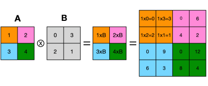
Figure 7: An illustration of Kronecker product on matrices $\mathbf{A}$ and $\mathbf{B}$.

(Kronecker product): Formally, as illustrated in Figure 7, given two matrices $\mathbf{A}\in\mathbbm{R}^{p\times q}$ and $\mathbf{B}\in\mathbbm{R}^{s\times t}$, the Kronecker product of $\mathbf{A}$ and $\mathbf{B}$ is defined as

$$\mathbf{A}\otimes\mathbf{B}=\begin{bmatrix}a_{1,1}\mathbf{B}&a_{1,2}\mathbf{B}&\cdots&a_{1,q}\mathbf{B}\\ a_{2,1}\mathbf{B}&a_{2,2}\mathbf{B}&\cdots&a_{2,q}\mathbf{B}\\ \vdots&\vdots&\ddots&\vdots\\ a_{p,1}\mathbf{B}&a_{p,2}\mathbf{B}&\cdots&a_{p,q}\mathbf{B}\\ \end{bmatrix}\in\mathbbm{R}^{ps\times qt},$$ (31)

where the output will be a larger matrix with $p\times s$ rows and $q\times t$ columns.

The Kronecker product can also be applied to vectors, with the base polynomial vectors $P_{0}(\mathbf{x})$ and $P_{1}(\mathbf{x})$, the other Taylor’s polynomials with higher orders can all be recursively defined as follows:

$$P_{d}(\mathbf{x})=P_{1}(\mathbf{x})\otimes P_{d-1}(\mathbf{x})\text{, for }\forall d\geq 2.$$ (32)

With the notation $P_{d}(\mathbf{x})$, we can define the Taylor’s polynomials based data expansion function as the list of polynomial terms with orders no greater than $d$ (where $d$ is a hyper-parameter of the function) as follows:

$$\kappa(\mathbf{x}|d)=[P_{1}(\mathbf{x}),\cdots,P_{d}(\mathbf{x})]\in\mathbbm{R}^{D}.$$ (33)

Since RPN has a deep architecture, the hyper-parameter $d$ is normally set to a small value (e.g., $d=2$) to avoid excessively large expansions at each layer. Expanding the input data to a Taylor’s polynomial of order $4$ can be achieved either by stacking two layers of RPN layer or by nesting two Taylor’s expansion functions with $d=2$. Additionally, the base term $P_{0}(\mathbf{x})$ containing the constant value ‘$1$’ can be subsumed by the bias term in the inner product implementation, and thus need not be explicitly included in the expansion. The output dimension will then be $D=\sum_{i=1}^{d}m^{i}$.

Taylor’s polynomials are known to approximate functions very well, and an illustrative example of their approximation correctness on function $y=\exp(x)$ is provided below.

Example: In the right plot, we illustrate the approximation of function $f(x)=\exp(x)$ with Taylor’s polynomials of different orders, where the notation $T_{d}(x)$ denotes the Taylor’s polynomials with degrees up to $d$. According to the plot, increasing the degree allows the Taylor’s polynomials to approximate the function $f(x)$ more accurately. Among all these illustrated Taylor’s polynomials in the plot, $T_{4}(x)=1+x+\frac{x^{2}}{2}+\frac{x^{3}}{6}+\frac{x^{4}}{24}$ outperforms the others.

5.1.4 Fourier Series based Data Expansions

A Fourier series is an expansion of a periodic function into the sum of Fourier series. In mathematics, the Dirichlet-Jordan test gives sufficient conditions for a real-valued, periodic function to be equal to the sum of its Fourier series at a point of continuity. Fourier series can be represented in several forms, and in this paper, we will utilize the sine-cosine representation.

Based on the hyper-parameters $P$ and $N$, we can represent the Fourier series based data expansion function $\kappa$ for the input vector $\mathbf{x}$ as follows:

$$\kappa(\mathbf{x}|P,N)=\left[\cos(2\pi\frac{1}{P}\mathbf{x}),\sin(2\pi\frac{1}{P}\mathbf{x}),\cos(2\pi\frac{2}{P}\mathbf{x}),\sin(2\pi\frac{2}{P}\mathbf{x}),\cdots,\cos(2\pi\frac{N}{P}\mathbf{x}),\sin(2\pi\frac{N}{P}\mathbf{x})\right]\in\mathbbm{R}^{D},$$ (34)

where the output dimension $D=2mN$.

5.1.5 B-Splines based Data Expansion

Formally, a B-spline of degree $d+1$ is defined as a collection of piecewise polynomial functions $\left\{B_{i,d}(x)\right\}_{i\in\{0,2,\cdots,t-1\}}$ of degree $d$ over the variable $x$, which takes values from a pre-defined value range $[x_{0},x_{t})$. The value range $[x_{0},x_{t}]$ is divided into smaller pieces by points $x_{0},x_{1},x_{2},\cdots,x_{t}$ sorted in a non-decreasing order, and these points are also known as the knots. These knots partition the value range $[x_{0},x_{t}]$ into $t$ disjoint intervals: $[x_{0},x_{1}),[x_{1},x_{2}),\cdots,[x_{t-1},x_{t})$.

As to the specific representations of B-splines, they can be defined recursively based on the lower-degree terms according to the following equations:

Base B-splines with degree $d=0$:

$$\left\{B_{0,0}(x),B_{1,0}(x),\cdots,B_{t-1,0}(x)\right\},$$ (35)

where

$$B_{i,0}(x)=\begin{cases}1,&\text{if }x_{i}\leq x<x_{i+1};\\ 0,&\text{otherwise}.\end{cases}$$ (36)

Higher-degree B-splines with $d>0$:

$$\left\{B_{0,d}(x),B_{1,d}(x),\cdots,B_{t-1,d}(x)\right\},$$ (37)

where

$$B_{i,d}(x)=\frac{x-x_{i}}{x_{i+d}-x_{i}}B_{i,d-1}(x)+\frac{x_{i+d+1}-x}{x_{i+d+1}-x_{i+1}}B_{i+1,d-1}(x).$$ (38)

According to the representations, term $B_{i,d}(x)$ recursively defined above will have non-zero outputs if and only if the inputs lie within the value range $x_{i}\leq x<x_{i+d+1}$.

B-splines have been extensively used in curve-fitting and numerical differentiation of experimental data, including their recent application in the design of KAN [Liu2024KANKN]. In this paper, we define the B-spline-based data expansion function with degree $d$, which can be represented as follows:

$$\kappa(\mathbf{x}|d)=\left[B_{0,d}(\mathbf{x}),B_{1,d}(\mathbf{x}),\cdots,B_{t-1,d}(\mathbf{x})\right]\in\mathbbm{R}^{D},$$ (39)

where the output dimension can be calculated as $D=m(t+d)$.

5.1.6 Chebyshev Polynomials based Data Expansion

In addition to B-splines, we observe several other similar basis functions recursively defined based on those of lower degrees, including Chebyshev polynomials and Jacobi polynomials.

Chebyshev polynomials have been demonstrated to be important in approximation theory for the solution of linear systems. They can be represented as two sequences of polynomials related to the cosine and sine functions (also known as the first-kind and second-kind), with recursive calculation equations that are quite similar to each other, differing only in scalar coefficients. In this paper, we will use the Chebyshev polynomials of the first kind (i.e., defined based on the cosine function) and it can be represented with the following recursive equations.

Base cases $d=0$ and $d=1$:

$$T_{0}(x)=1\text{, and }T_{1}(x)=x$$ (40)

High-order cases with degree $d\geq 2$:

$$T_{d}(x)=2x\cdot T_{d-1}(x)-T_{d-2}(x).$$ (41)

Based on the above representations, in this paper, we define the Chebyshev polynomials based data expansion function with degree hyper-parameter $d\geq 1$ as follows:

$$\kappa(\mathbf{x}|d)=\left[T_{1}(\mathbf{x}),T_{2}(\mathbf{x})\cdots,T_{d}(\mathbf{x})\right]\in\mathbbm{R}^{D}.$$ (42)

Similar to the aforementioned Taylor’s polynomial-based data expansions, since the output of $T_{0}(x)$ is a constant, it will not be included in the expansion function definition by default, and the output dimension will be $D=md$.

5.1.7 Jacobi Polynomials based Data Expansion

Different from the Chebyshev polynomial, the Jacobi polynomials have a more complicated recursive representation. Formally, the Jacobi polynomials parameterized by $\alpha$ and $\beta$ of degree $d\geq 2$ on variable $x$ can be represented as $P_{d}^{(\alpha,\beta)}(x)$, which can be recursively defined based on the lower-order cases:

$$P_{d}^{(\alpha,\beta)}(x)= \frac{(2d+\alpha+\beta-1)\left[(2d+\alpha+\beta)(2d+\alpha+\beta-2)x+(\alpha^{2}-\beta^{2})\right]}{2d(d+\alpha+\beta)(2d+\alpha+\beta-2)}P_{d-1}^{(\alpha,\beta)}(x)$$ (43)

$$-\frac{2(d+\alpha-1)(d+\beta-1)(2d+\alpha+\beta)}{2d(d+\alpha+\beta)(2d+\alpha+\beta-2)}P_{d-2}^{(\alpha,\beta)}(x).$$

As to the base case, we list some of them as follows:

$$P_{0}^{(\alpha,\beta)}(x) =1,$$ (44)

$$P_{1}^{(\alpha,\beta)}(x) =(\alpha+1)+(\alpha+\beta+2)\frac{(x-1)}{2},$$

$$P_{2}^{(\alpha,\beta)}(x) =\frac{(\alpha+1)(\alpha+2)}{2}+(\alpha+2)(\alpha+\beta+3)\frac{x-1}{2}+\frac{(\alpha+\beta+3)(\alpha+\beta+4)}{2}\left(\frac{x-1}{2}\right)^{2}.$$

In this paper, we define the Jacobi polynomial based data expansion function with degree $d$ as follows:

$$\kappa(\mathbf{x}|d)=\left[P_{1}^{(\alpha,\beta)}(\mathbf{x}),P_{2}^{(\alpha,\beta)}(\mathbf{x}),\cdots,P_{d}^{(\alpha,\beta)}(\mathbf{x})\right]\in\mathbbm{R}^{D},$$ (45)

where the output dimension $D=md$.

The Jacobi polynomials belong to the family of classic orthogonal polynomials, where two different polynomials in the sequence are orthogonal to each other under some inner product. Meanwhile, the Gegenbauer polynomials form the most important class of Jacobi polynomials, and Chebyshev polynomial is a special case of the Gegenbauer polynomials. In addition to these, we will also gradually incorporate other classic orthogonal polynomials into our tinyBIG toolkit.

5.1.8 Hyperbolic Function and Trigonometric Function based Data Expansions

The Fourier series introduced above is actually an example of a trigonometric series. In addition to Fourier series, we also include several other types of trigonometric functions based data expansion approach in this paper, such as hyperbolic functions, shown as follows:

$$\kappa(\mathbf{x})=\left[\cosh(\mathbf{x}),\sinh(\mathbf{x}),\tanh(\mathbf{x})\right]\in\mathbbm{R}^{D}\text{, where }D=3m.$$ (46)

In addition to the hyperbolic functions, we can also define the data expansion function using inverse hyperbolic functions, trigonometric functions, and inverse trigonometric functions, as follows:

$$\kappa(\mathbf{x}) =\left[\text{arccosh}(\mathbf{x}),\sinh(\mathbf{x}),\tanh(\mathbf{x})\right]\in\mathbbm{R}^{D};$$ (47)

$$\kappa(\mathbf{x}) =\left[\cos(\mathbf{x}),\sin(\mathbf{x}),\tan(\mathbf{x})\right]\in\mathbbm{R}^{D};$$ (48)

$$\kappa(\mathbf{x}) =\left[\arccos(\mathbf{x}),\arcsin(\mathbf{x}),\arctan(\mathbf{x})\right]\in\mathbbm{R}^{D},$$ (49)

where the output dimensions of these expansion functions are all $D=3m$.

Unlike hyperbolic functions, trigonometric functions are periodic, and different input values of $x$ may be projected to identical outputs, rendering them indistinguishable. This can potentially lead to degraded performance. Nonetheless, the above trigonometric function-based data expansion function can be employed as intermediate layers or complementary heads within a layer to compose more complex functions and construct more powerful models.

5.1.9 Radial Basis Functions based Data Expansion

In mathematics, a radial basis function (RBF) is a real-valued function $\varphi$ defined based on the distance between the input ${x}$ and some fixed point, e.g., ${c}$, which can be represented as follows:

$$\varphi({x}|c)=\varphi(x-c).$$ (50)

There are different ways to define the function $\varphi$ in practice, two of which studied in this paper are shown as follows:

$$\underline{\textbf{(a) Gaussian RBF:}}$$ (51)

$$\varphi(x|c)=e^{-(\epsilon(x-c))^{2}},$$

$$\text{ where }\epsilon\text{ is a hyperparameter}.$$

$$\underline{\textbf{(b) Inverse Quadratic RBF:}}$$ (52)

$$\varphi(x|c)=\frac{1}{1+(\epsilon(x-c))^{2}},$$

$$\text{ where }\epsilon\text{ is a hyperparameter}.$$

Given a set of $d$ different fixed points, e.g., $\mathbf{c}=[c_{1},c_{2},\cdots,c_{d}]$, a sequence of $d$ different such RBF can be defined, which compare the input against these $d$ different fixed points shown as follows:

$${\varphi}(x|\mathbf{c})=\left[\varphi(x|c_{1}),\varphi(x|c_{2}),\cdots,\varphi(x|c_{d})\right]\in\mathbbm{R}^{d}.$$ (53)

With the above notations, we can represent the Gaussian RBF and Inverse Quadratic RBF based data expansion functions both with the following equation:

$$\kappa(\mathbf{x})={\varphi}(\mathbf{x}|\mathbf{c})=\left[\varphi(\mathbf{x}|c_{1}),\varphi(\mathbf{x}|c_{2}),\cdots,\varphi(\mathbf{x}|c_{d})\right]\in\mathbbm{R}^{D},$$ (54)

where the output dimension will be $D=md$.

5.1.10 Combinatorial Data Expansion

Combinatorial data expansion function expands input data by enumerating the potential combinations of elements from the input vector, with the number of elements to be combined ranging from $1$, $2$, $\cdots$, $d$, where $d$ is a hyper-parameter. Formally, given a data instance featured by a variable set $\mathcal{X}=\{X_{1},X_{2},\cdots,X_{m}\}$ (here, we use the upper-case $X_{i}$ to denote the variable of the $i_{th}$ feature), we can represent the possible combinations of $d$ terms selected from $\mathcal{X}$ with notation:

$${\mathcal{X}\choose d}=\left\{\mathcal{C}|\mathcal{C}\subset\mathcal{X}\land|\mathcal{C}|=d\right\},\\$$ (55)

where $\mathcal{C}$ denotes a subset of $\mathcal{X}$ containing no duplicated elements and the size of the output set ${\mathcal{X}\choose d}$ will be equal to ${m\choose d}$. Some simple examples with $d=1$, $d=2$ and $d=3$ are illustrated as follows:

$$d=1: {\mathcal{X}\choose 1}=\left\{\{X_{i}\}|X_{i}\in\mathcal{X}\right\},$$ (56)

$$d=2: {\mathcal{X}\choose 2}=\left\{\{X_{i},X_{j}\}|X_{i},X_{j}\in\mathcal{X}\land X_{i}\neq X_{j}\right\},$$

$$d=3: {\mathcal{X}\choose 3}=\left\{\{X_{i},X_{j},X_{k}\}|X_{i},X_{j},X_{k}\in\mathcal{X}\land X_{i}\neq X_{j}\land X_{i}\neq X_{k}\land X_{j}\neq X_{k}\right\}.$$

By applying the above notations to concrete data instances, given a data instance with values $\mathbf{x}=[x_{1},x_{2},\cdots,x_{m}]$ (the lower-case $x_{i}$ denotes the feature value), we can also represent the combinations of $d$ selected features from $\mathbf{x}$ as ${\mathbf{x}\choose d}$, which can be used to define the combinatorial data expansion function as follows:

$$\kappa(\mathbf{x})=\left[{\mathbf{x}\choose 1},{\mathbf{x}\choose 2},\cdots,{\mathbf{x}\choose d}\right].$$ (57)

Similar as the above Taylor’s expansions, the output dimension of the combinatorial expansion will increase exponentially. Given an input data vector $\mathbf{x}\in\mathbbm{R}^{m}$, with hyper-parameter $d$, its expansion output of combinations with up to $d$ elements will be $\kappa(\mathbf{x})\in\mathbbm{R}^{D}$, where $D=\sum_{i=1}^{d}i\cdot{m\choose i}$.

5.1.11 Probabilistic Data Expansion

An important category of data expansion functions that surprisingly performed very well, even outperforming many of the extension approaches mentioned above, are probability density function based data expansions. Formally, in probability theory and statistics, a probability density function (PDF) is a function that describes the relative likelihood for a random variable to take on a given value within its sample space. Formally, given a probabilistic distribution parameterized by $\theta$, we can represent its probability density function as

$$P(x|\theta)\in[0,1]\text{, where }\int_{x}P(x|\theta)\mathrm{d}x=1.$$ (58)

Lots of probabilistic distributions have been proposed by mathematicians and statisticians, such as Gaussian distribution $\mathcal{N}(\mu,\sigma)$, Exponential distribution $\mathcal{E}(\lambda)$, Laplace distribution $\mathcal{L}(\mu,b)$, Cauchy distribution $\mathcal{C}(x_{0},\gamma)$, Chi-squared distribution $\mathcal{X}^{2}(k)$ and Gamma distribution $\Gamma(k,\theta)$, etc. The PDFs of these distributions are also provided as follows:

$$\underline{\textbf{(a) Gaussian Distribution:}}$$ (59)

$$P(x|\mu,\sigma)=\frac{1}{\sigma\sqrt{2\pi}}\exp^{-\frac{1}{2}(\frac{x-\mu}{\sigma})^{2}},$$

$$\text{ where }\mu,\sigma\text{ are the mean and std parameters}.$$

$$\underline{\textbf{(b) Exponential Distribution:}}$$ (60)

$$P(x|\lambda)=\begin{cases}\lambda\exp^{-\lambda x}&\text{ for }x\geq 0,\\ 0&\text{ otherwise},\end{cases},$$

$$\text{ where }\lambda>0\text{ is the rate parameter}.$$

$$\underline{\textbf{(c) Laplace Distribution:}}$$ (61)

$$P(x|\mu,b)=\frac{1}{2b}\exp^{\left(-\frac{|x-\mu|}{b}\right)},$$

$$\text{ where }\mu,b>0\text{ are the location, scale parameters}.$$

$$\underline{\textbf{(d) Cauchy Distribution:}}$$ (62)

$$P(x|x_{0},\gamma)=\frac{1}{\pi\gamma\left[1+\left(\frac{x-x_{0}}{\gamma}\right)^{2}\right]},$$

$$\text{ where }x_{0},\gamma\text{ are the location and scale parameters}.$$

$$\underline{\textbf{(e) Chi-Squared Distribution:}}$$ (63)

$$P(x|k)=\frac{1}{2^{\frac{k}{2}}\Gamma(\frac{k}{2})}x^{(\frac{k}{2}-1)}\exp^{-\frac{x}{2}},$$

$$\text{ where }k\in\mathbbm{N}^{+}\text{ is the dof parameter}.$$

$$\underline{\textbf{(f) Gamma Distribution:}}$$ (64)

$$P(x|k,\theta)=\frac{1}{\Gamma(k)\theta^{k}}x^{k-1}\exp^{-\frac{x}{\theta}},$$

$$\text{ where }k,\theta>0\text{ are the shape and scale parameters}.$$

When feeding inputs to a probability density function, its output is typically a very small number, and the curve of many distribution PDFs can be quite flat (i.e., with a very small slope). In this paper, we propose using the log-likelihood to expand the input data instead, which makes it possible to unify the representations of probabilistic graphical models with RPN, more information of which will be introduced in Section LABEL:subsec:pm.

In this paper, we introduce two different expansions based on the probabilistic distributions, i.e., naive probabilistic expansion and combinatorial probabilistic expansion introduced as follows.