Thermalization in Trapped Bosonic Systems With Disorder

Abstract

A detailed study of thermalization is conducted on experimentally accessible states in a system of bosonic atoms trapped in an open linear chain with disorder. When the disorder parameter is large, the system exhibits regularity and localization. In contrast, weak disorder introduces chaos and raises questions about the validity of the Eigenstate Thermalization Hypothesis (ETH), especially for states at the extremes of the energy spectrum which remain regular and non-thermalizing.

The validity of ETH is assessed by examining the dispersion of entanglement entropy and the number of bosons on the first site across various dimensions, while maintaining a constant particle density of one. Experimentally accessible states in the occupation basis are categorized using a crowding parameter that linearly correlates with their mean energy.

Using full exact diagonalization to simulate temporal evolution, we study the equilibration of entanglement entropy, the number of bosons, and the reduced density matrix of the first site for all states in the occupation basis. Comparing equilibrium values of these observables with those predicted by microcanonical ensembles, we find that, within certain tolerances, most states in the chaotic region thermalize. However, states with low participation ratios in the energy eigenstate basis show greater deviations from thermal equilibrium values.

I Introduction

In recent years, experiments with ultracold atomic systems confined to one-dimensional (1D) geometries have emerged as a frontier in quantum statistical mechanics [1, 2, 3, 4, 5]. The properties of these systems, governed by the laws of quantum mechanics, present profound challenges to our traditional understanding of statistical ensembles and equilibrium states. These experiments, often conducted at ultra-low temperatures near absolute zero, allow researchers unprecedented control over individual quantum states, enabling them to probe phenomena that were previously inaccessible[6, 7, 8]. Despite the remarkable progress in experimental techniques and theoretical frameworks, fundamental questions persist regarding the applicability of conventional statistical ensembles in describing the behavior of these few-particle systems[9, 10]. In particular, the validity of canonical and microcanonical ensembles in capturing the thermalization processes of such systems remains an open question. Addressing these challenges requires a comprehensive investigation into the intricate interplay between quantum coherence, particle interactions, and external confinement, shedding light on the fundamental principles underlying the behavior of quantum many-body systems in low-dimensional geometries. This study aims to contribute to this dialogue by examining the thermalization dynamics of bosonic atoms trapped in a disordered 1D chain, offering insights into the fundamental mechanisms governing the thermalization of quantum systems at the nanoscale.

Thermalization processes in quantum systems have witnessed significant breakthroughs, leading to the formulation of the Eigenstate Thermalization Hypothesis (ETH), a pivotal concept reshaping our perception of quantum dynamics [11, 12, 13]. The ETH posits that eigenstates of typical quantum Hamiltonians exhibit statistical properties similar to those predicted by the microcanonical ensemble, fundamentally implying that the system’s behavior can be effectively described by equilibrium statistical mechanics. This paradigm shift has profound implications, not only for fundamental quantum theory but also for practical applications in areas such as quantum information and condensed matter physics. In the context of this article, we demonstrate the validity of the ETH within the framework of the Aubry-André model, showcasing its robustness and applicability across diverse quantum systems.

Our study is motivated by the desire to provide experimental scientists with guidance on the long-term behavior of states in the occupation basis, which have been extensively studied and realized in experiments involving ultra-cold atoms. These experimental platforms offer a unique opportunity to probe and validate theoretical predictions concerning thermalization processes in quantum systems. By focusing on the behavior of occupation states over extended time scales, we aim to offer insights that can inform experimentalists about the dynamics and evolution of these states under various conditions. Through a comprehensive analysis, we not only aim to validate the ETH but also to provide a roadmap for experimental investigations into the thermalization dynamics of these states.

The paper is structured as follows: In Section II we introduce the Hamiltonian of the system, discuss its basic properties, particularly the quantum signatures of chaos in its spectrum, and also discuss some properties of the occupation basis, which are the initial states considered in this contribution. Section III.1 presents the probabilities of occupation and highlights these as principal observables commonly measured in experiments. Moving on to Section III.2, we scrutinize the validity of the ETH through the lens of two specific observables: the entanglement entropy and the number of bosons in the first site. Throughout all section IV, the equilibrium values of the observables for initial states in the occupation basis are compared with those obtained from a microcanonical ensemble. Conclusions drawn from our analysis are presented in Section V.

II The Interacting Aubry-André model (IAA)

The Interacting Aubry-André model (IAA) describes the dynamics of $N$ spin-less bosons on a lattice with $M$ sites in a one dimensional chain with open boundary conditions. The Hamiltonian of this system, with $\hbar=1$, is

$$\hat{H}=-J\sum_{\braket{i,j}=1}^{M}\hat{b}_{i}^{\dagger}\hat{b}_{j}+\frac{U}{2}\sum_{i=1}^{M}\hat{n}_{i}(\hat{n}_{i}-1)+W\sum_{i=1}^{M}\cos(2\pi\beta i+\phi)\hat{n}_{i}$$ (1)

The operators $\hat{b}^{\dagger}_{i}$ and $\hat{b}_{i}$ are the creation and annihilation operators of one boson on the site $i$, respectively. The first term describes the coherent tunneling coupling between neighboring lattice sites with rate $J$. The second term represents the interaction between bosons, depending on the occupancy, $\hat{n}_{i}=\hat{b}_{i}^{\dagger}\hat{b}_{i}$, in the same site $i$. The last term introduces a site disorder, with an incommensurate frequency $\beta$, phase $\phi$, and disorder parameter $W$. The Hamiltonian parameters $J$, $W$ and $\phi$ can be controlled by the experimentalists, nevertheless, the phase $\phi$ can vary randomly from one realization to another.

The dimension of the Hilbert space of the system is determined by the expression Dim $=(N+M-1)!/N!(M-1)!$, where $N$ and $M$ are the number of bosons and sites, respectively. In this study, considering a unit filling of the lattice ($N/M=1$), we investigate four different lattice sizes: $M=7,8,9,10$, corresponding to Hilbert space dimensions of $1716$, $6435$, $24310$, and $92378$, respectively. The dynamics of the observables are calculated using full exact diagonalization. Each system size is sampled in 40 realizations by considering random values of $\phi$ in the range $[0,2\pi)$, following the approach outlined in [14]. Most observables are calculated as averages over these $40$ realizations with random $\phi$, in order to highlight some quantum phenomena

When the disorder parameter $W$ in the Hamiltonian is significantly large (1), it disrupts the thermalization process and many-body localization (MBL) occurs. This results in the cessation of transport and bosons become localized. The transition to this localized state is highly dependent on the parameter $\beta$, which is chosen ideally as an irrational number. In practical experiments, $\beta$ is frequently associated to the wavelengths of a pair of lasers. In this study, we employ a decimal approximation to the golden ratio $\beta=1.618$, whereas for the remaining parameters we consider $U=4/(N-1)$, $J=1/2$, and $W=0.6$[5]. These parameter values are associated with the presence of chaos and a richer dynamics in the system, as previously observed in studies such as [15, 16, 17, 18]. The dependence of $U$ with $N$ guarantees that all terms in the Hamiltonian scale with $N$ in the same way.

II.1 Spectral signatures of quantum chaos

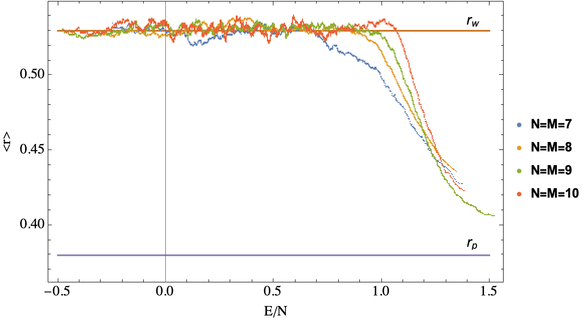
Figure 1: Averaged level spacing ratio $\braket{r}$ is shown for different system sizes. The upper and lower horizontal lines show the limits $r_{W}=0.53$, and $r_{P}=0.38$ which correspond to values of $\braket{r}$ for Wygner-Dyson and Poison distribution respectively.

Commonly used indicators of quantum chaos rely on the properties of the energy spectrum, and determine how close is this spectrum to that of an ensemble of random matrices. For a sorted set of eigenenergies, denoted as $E_{n}$ (with $n=1,2,...,\text{Dim}$), the spacing between nearest neighbors, $s_{n}=E_{n+1}-E_{n}$, show two different distributions. Quantum chaotic systems exhibit level spacing that follows the Wigner-Dyson distribution, whose main characteristic is the level repulsion ($\lim_{\tilde{s}\rightarrow 0}P(\tilde{s})=0$.) For the Gaussian Orthogonal Ensamble (GOE), it is [19]

$$P(\tilde{s})=\frac{\tilde{s}}{2\sigma^{2}}e^{-\tilde{s}^{2}/4\sigma^{2}},$$ (2)

in terms of the unfolded variable $\tilde{s}=s/\Delta E$, being $1/\Delta E$ the density of states.

Conversely, in regular systems where eigenvalues are not correlated, the distribution of level spacing aligns well with the Poisson distribution.

$$p(\tilde{s})=e^{-\tilde{s}}.$$ (3)

In order to elude the unfolding procedure, one can use the ratio of two consecutive level spacings, a method proposed by Oganesyan and Huse[20, 21, 22],

$$\tilde{r}=\frac{\text{min}(s_{n},s_{n-1})}{\text{max}(s,s_{n-1})}=\text{min}\left(r_{n},\frac{1}{r_{n}}\right)$$ (4)

with $r_{n}=s_{n}/s_{n-1}$. This ratio is independent of the density of states and, as said before, no unfolding is necessary. For quantum chaotic systems, the mean level spacing ratio is $\langle\tilde{r}\rangle_{W}=4-2\sqrt{3}\approx 0.535$, whereas for regular systems, it has a lower mean value of $\langle\tilde{r}\rangle_{P}=2\ln 2-1\approx 0.386$ [23, 24].

Fig. 1 illustrates the level spacing ratio $\langle r\rangle$ versus the mean energy of the levels in intervals of 200 energy states for the IAA model, averaged over 40 realizations and for four different system sizes. The chaotic region extends from $E/N=-0.5$ to $E/N\approx 0.7$ for $M=7$, whereas for larger system sizes the upper chaotic limit increases up to $E/N\approx 1.1$ for $M=10$. In all cases, for high-energy states, the system transitions to a regular spectrum.

II.2 Occupation basis

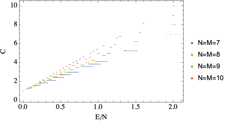
Figure 2: Crowding parameter versus energy of occupation states.

In this contribution we consider all the elements of the occupation basis as initial states. The occupation basis provides a convenient representation where the states of the system are described by the number of bosons present at each site of the lattice. The occupation basis is defined as follows: consider a one-dimensional lattice with $M$ sites, labeled by $i=1,2,…,M$. Let there be a total of $N$ bosons in the system. An occupation state is denoted by $\ket{\mathbf{n}}\equiv\ket{n_{1},n_{2},...,n_{M}}$, where $n_{i}$ represents the number of bosons at site $i$. The total number of bosons is conserved, hence:

$$\sum_{i=1}^{M}n_{i}=N.$$ (5)

The occupation states form a complete basis for the Hilbert space of the system.

A categorization of all potential initial states in the occupation basis is established by introducing a parameter that we call the crowding parameter

$$C=\frac{1}{N}\sum{n_{i}^{2}}.$$ (6)

The crowding parameter varies from 1 (representing a state where each site contains one particle) to $N$ (representing a state where all particles are situated in a single site).

The crowding parameter is associated with the expectation value of the energy for occupation states. Observe that, since the hopping term has no diagonal components in the occupation basis, and the disorder term is an oscillatory function of the phase $\phi$ with null average over many realizations, the average energy of the occupation states has only contributions from the interaction term [the second one in the Hamiltonian of Eq. (1)]. For this reason, the average value of the energy for occupation states is linear in the crowding parameter $E=\bra{\mathbf{n}}H\ket{\mathbf{n}}\approx\frac{U}{2}N(C-1)$. This linear behavior is observed in Fig. 2. Notice that the energy width at each value of C becomes visibly smaller as N increases.

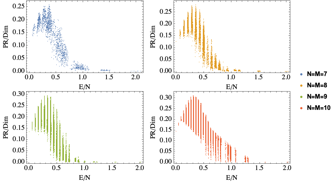
Figure 3: Participation Ratio (PR), normalized by the dimension Dim of the Hilbert space, vs the expectation value of energy for occupation states and for different sizes of the system.

II.3 Localization of the occupation states in the Hamiltonian eigenbasis

A relevant property for anticipating the dynamical behaviour of an initial state is its distribution in the Hamiltonian eigenbasis. A simple characterization of this distribution is obtained by calculating the Participation Ratio (PR).

The Participation Ratio serves as an efficient measure of how many states (of an arbitrary basis $\{\ket{\phi_{m}}\}$) are needed to built a given state $\ket{k}=\sum_{m}c^{(k)}_{m}\ket{\phi_{m}}$. It is defined as

$$\mathrm{PR}_{k}=\frac{1}{\sum_{m}|c^{(k)}_{m}|^{4}}.$$ (7)

A low PR value indicates that the state is highly localized, meaning it is predominantly composed of a few basis states. Conversely, a high PR value suggests that the state is spread out across many basis states, indicating delocalization.

Fig. 3 presents the PR of all occupation states in the eigenbasis, plotted versus their average energy $E$. Note that the occupation states accommodate in several clusters with approximately the same energy, these clusters are associated to the different values of the crowding parameter as can be clearly seen in Fig.2. It can be observed that most occupation states, whose energies lie in region $E/N<0.5$ have $\mathrm{PR}>0.10$Dim, i.e., are the more delocalized in the eigenbasis. On the other hand, those states with larger crowding parameters have the highest energies and the lowest PRs.

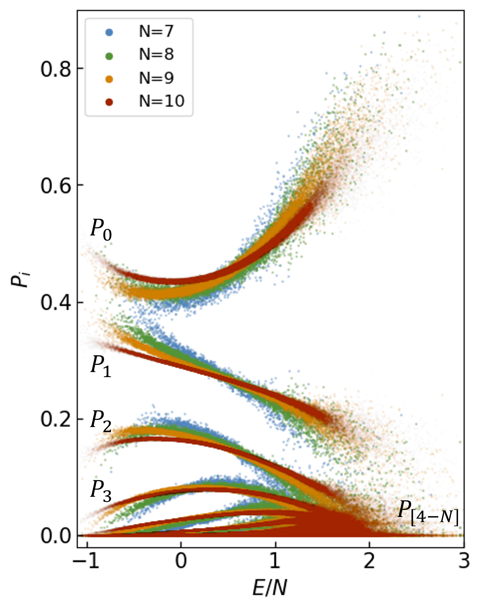
Figure 4: Eigenstate expectation values of occupation probabilities at the first site.

III Thermalization in the IAA model: static properties

The Eigenstate Termalization Hyphothesis (ETH) [13] postulates that the expectation value $\bra{\phi_{m}}\hat{A}\ket{\phi_{m}}$ of any operator will be approximately the same for most of the eigenstates $\ket{\phi_{m}}$ with energies $E_{m}$ in a small energy window $\Delta E$. It implies that generic states whose components in the eigenbasis are concentrated in this energy region will all attain the same temporal average of this observable.

III.1 Occupation probabilities

The occupation probabilities are the observables most commonly found in the experiments. They are defined as the probability to find $i$ particles in a determinate site of the chain. For any state $\ket{q}=\sum_{n_{1},n_{2},...,n_{M}}c^{(q)}_{n_{1},n_{2},...,n_{M}}\ket{n_{1},n_{2},...,n_{M}}$, the probability $P^{(q)}_{i}$ of finding $i$ bosons, $i=0,1,2,...,N$, in the first site is

$$P^{(q)}_{i}=\sum_{n_{2},...,n_{M}}|c^{(q)}_{n_{1}=i,n_{2},...,n_{M}}|^{2}.$$ (8)

$i$	0	1	2	3	4	5	6	7	8
$N_{i}$	3003	1716	924	462	210	84	28	7	1
$p_{i}$	0.46667	0.26667	0.14359	0.07179	0.03263	0.01305	0.00435	0.001091	0.00016

Table 1: The second row list the number of states $N_{i}$ with occupation number $i$ in the occupation basis, with $i$ in the first row. The third row lists $p_{i}\equiv N_{i}/6435$, where $6435$ is the number of states for $N=8$ bosons in $L=8$ sites.

The figure 4 presents the average over 40 realizations of the occupation probabilities for the eigenstates of the IAA model. Notably, across all dimensions, the probability of finding zero particles in the first site is notably elevated, and the occupation probability of finding larger number of particles decreases as function of this number. This behaviour can be roughly understood by considering the whole occupation basis. The number and fraction of members of this basis with a given number of particles in a given site are shown in Table 1. The fractions and numbers of states show the same pattern: the largest set of states is that corresponding to zero particles in the given site, and the fractions decrease for states with a larger number of particles in the given site.

Moreover, as we move towards the edges of the spectrum, we observe, in figure 4, an increase in dispersion, whereas within the chaotic region, the observables display reduced dispersion. Importantly, for this chaotic region the dispersion reduces as the number of particles (and sites) increases, providing a first indication of thermalization of the system’s eigenstates.

III.2 Thermalization test for the number of particles and entanglement entropy

We have selected two observables, whose expectation values are calculated in the IAA model and, as in the case of occupation probabilities, are averaged over 40 realizations of the phase $\phi$ in the Hamiltonian 1. They are the expectation value of the number of atoms in the first site $\hat{n}_{1}$, and the Entanglement Entropy $S_{1}$ between the first site and the rest of the chain [10]. In terms of the occupation probabilities these observables are

$$n^{(q)}_{1}=\sum_{i=0}^{N}i\,P^{(q)}_{i},\,\,\,\,\,\,\,\,\,\hbox{and}\,\,\,\,\,\,\,S^{(q)}_{1}=-\sum_{i=0}^{N}P^{(q)}_{i}\ln P^{(q)}_{i}.$$ (9)

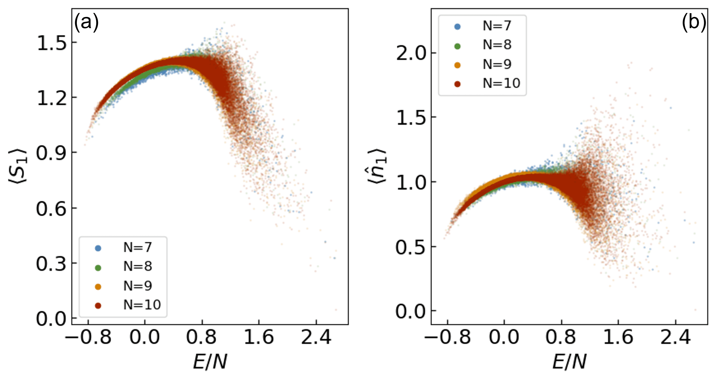
Figure 5: Two distinct observables in the eigenstates are depicted as a function of the energy values. (a) The entanglement entropy that measures the degree of entanglement between the first site and the remainder of the chain. (b) The expectation value of the particle number in the first site.

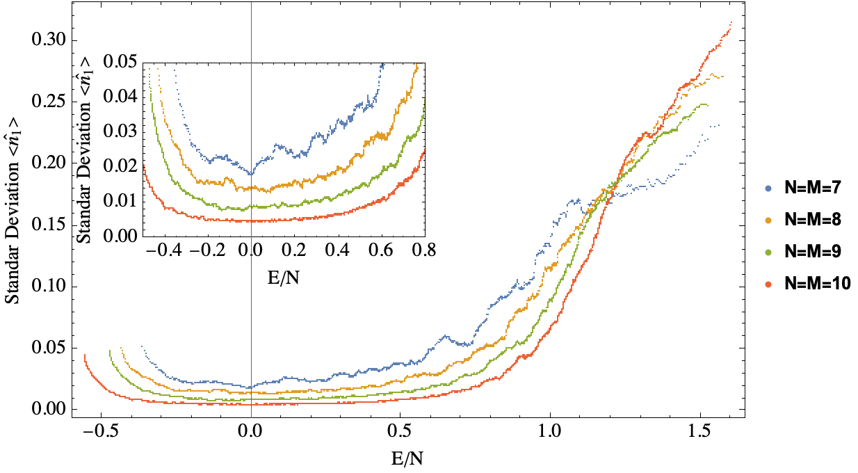
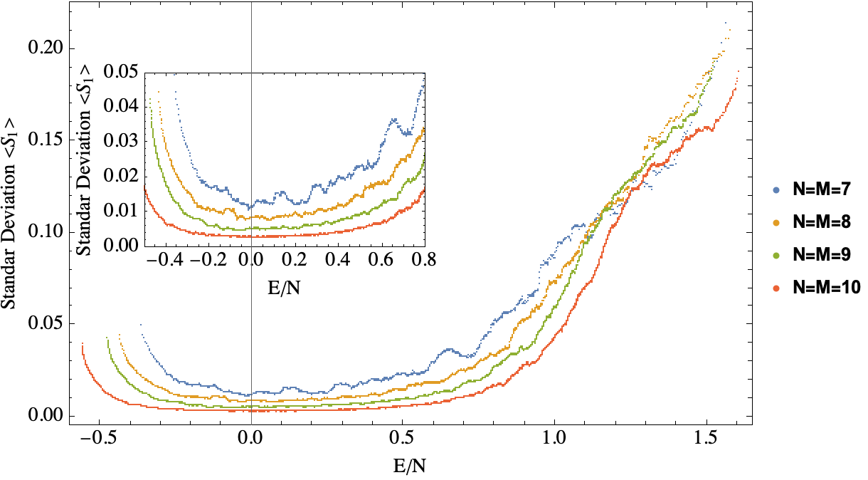
Figure 6: Standard deviation of averaged number of particles in the first site of the chain $\hat{n}_{1}$ for the eigenvectors taking a window of 200 states and standard deviation of the averaged entanglement entropy of the first site with the rest.

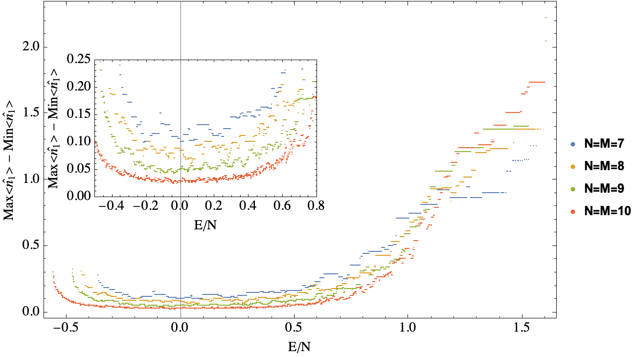
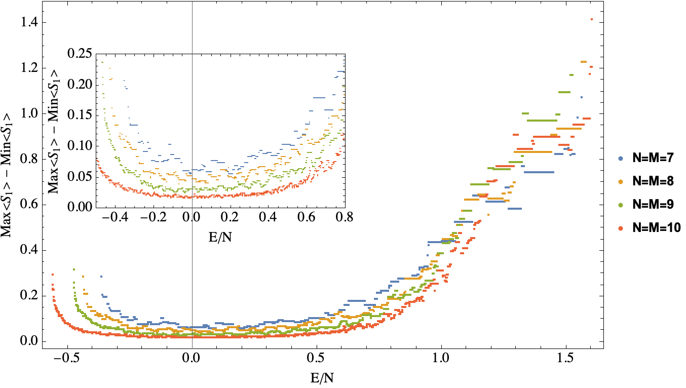
Figure 7: Top: maximun value of the averaged number of particles in the first site of the chain minus the minimun for windows of 200 eigenstates plotted versus the mean energy of the respective windows. Bottom: same as top panel, but now for the entanglement entropy of the first site respect to the rest of the chain.

Figure 5 illustrates the behavior of the average over 40 realizations of $\braket{n_{1}}$ for all eigenstates. It can be seen that eigenstates with energies lower than $E/N\lesssim 0.6$ satisfy the Eigenstate Thermalization Hypothesis (ETH): the average occupation exhibits a smooth dependence on $E/N$, with minimal dispersion for energies below $E/N\lesssim 0.6$. Additionally, the same figure displays the average entanglement entropy of the first site, $\braket{S_{1}}$, as a function of the average energy of each eigenstate. Similar to the occupation of first site, this observable presents a smooth behavior for energies below $E/N\lesssim 0.6$, whereas in the larger energy (regular) region, the dispersion is more pronounced across all dimensions.

To further demonstrate compliance with the Eigenstate Thermalization Hypothesis[25], Figures 6 and 7 show, respectively, the standard deviation and the maximum minus the minimum value of the entanglement entropy and the number of particles at site one as a function of the energy of the eigenstates for moving windows of 200 energy eigenstates. Four different sizes of the system are considered $N=M=7,8,9$ and $10$. It can be observed that, for energies below $E/N\lesssim 1.1$ and for the two observables, both dispersion measures diminish as the system size is increased, which is a strong test of the validity of the ETH for the same energy interval where quantum chaos was diagnosed in the model (see Fig.1).

IV Thermalization in the IAA model: dynamical properties

In the following, the equilibrium value of the observables for initial states in the occupation basis are compared with the microcanonical average to ascertain whether these observables exhibit thermalization behavior in the IAA model.

IV.1 Equilibrium values of initial states in the occupation basis.

Consider an isolated system initially prepared in a nonstationary state with a well-defined mean energy. In such a scenario, we characterize an observable as thermalizing if, throughout the system’s time evolution, it gradually approaches the microcanonical prediction and consistently remains close to it for the majority of subsequent times. Remarkably, whether the isolated system is in a pure or mixed state holds no significance in determining its thermalization behavior [26]. If we consider the time evolution of an isolated system, expanding the initial state in the eigenbasis of the Hamiltonian $\hat{H}$, $\ket{\Psi(0)}=\sum_{l}c_{l}\ket{\phi_{l}}$. The function at time $t$ evolves as $\ket{\Psi(t)}=e^{-i\hat{H}t}\ket{\Psi(0)}=\sum_{l}c_{l}e^{-iE_{l}t}\ket{\phi_{l}}$, with $E_{l}$ the eigenstate energies. The evolution of any observable $\hat{A}$ in quantum mechanics is described by the expression:

$$\hat{A}(t)=\braket{\Psi(t)}{\hat{A}}{\Psi(t)}=\sum_{m}|c_{m}|^{2}A_{mm}+\sum_{m,n\neq m}c_{m}^{*}c_{n}e^{i(E_{m}-E_{n})t}A_{mn},$$ (10)

where $A_{m,n}=\braket{\phi_{m}}{\hat{A}}{\phi_{n}}$. In the long-time average, the second sum in Eq. 10 typically averages to zero, provided there are no degeneracies or if their number is nonextensive. Consequently, we are left with the sum of the diagonal elements of $\hat{A}$ weighted by $|c_{m}^{2}|$.

The time evolution of the entanglement entropy of the first site $S_{1}$ is shown in Fig. 8 for two initial occupation states: $\ket{1,1,1,1,1,1,1,1}$ and $\ket{0,2,2,0,0,2,2,0}$. In both cases, $S_{1}$ exhibits small fluctuations around its equilibrium value at times larger than $100$. As this equilibration time can change depending on the initial state and the size of the system, in what follows we present equilibrium values of observables for $t=10^{4}$, averaged over 40 realizations of the model.

$S_{1}$

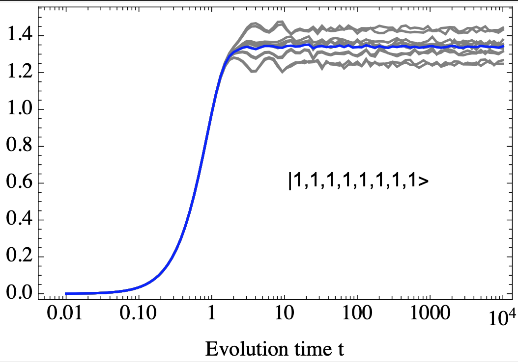
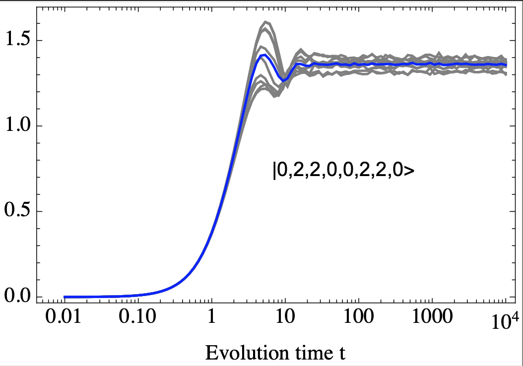
Figure 8: Time evolution of the entanglement entropy of the first site in the case $N=8$ $M=8$ for two different initial occupation states. Blue line is the average over 40 realizations. Gray lines show some examples of these realizations.

Thermalization of the observable $\hat{A}$ implies that the first term in Eq. 10 converges to the microcanonical average. The microcanonical average of a quantum observable $\hat{A}$ is defined as the average value of the observable over all the states within a specific energy range around a given energy $E$, this can be expressed as:

$$\langle\hat{A}\rangle_{\text{micro}}=\frac{1}{\mathcal{N}(E,\Delta E)}\sum_{E_{i}\in[E-\Delta E,E+\Delta E]}\langle\phi_{i}|\hat{A}|\phi_{i}\rangle$$ (11)

where $\mathcal{N}(E,\Delta E)$ is the number of quantum states $\ket{\phi_{i}}$ with energies within the range $[E-\Delta E,E+\Delta E]$, and $\braket{\phi_{i}}{\hat{A}}{\phi_{i}}$ is the expectation values of the observables $\hat{A}$ in the state $\ket{\phi_{i}}$.

In simpler terms, the microcanonical average is the mean value of the observable taken over all quantum states whose energies lie within a narrow interval centered around the energy $E$. This average is used to describe the behavior of the observable in equilibrium, assuming that the system is isolated and has a fixed energy. The microcanonical average was computed using a window centered on energy $E$, with 30 eigenstates to the right and left of this energy value. The window was shifted across the entire spectrum in increments of 1 state.

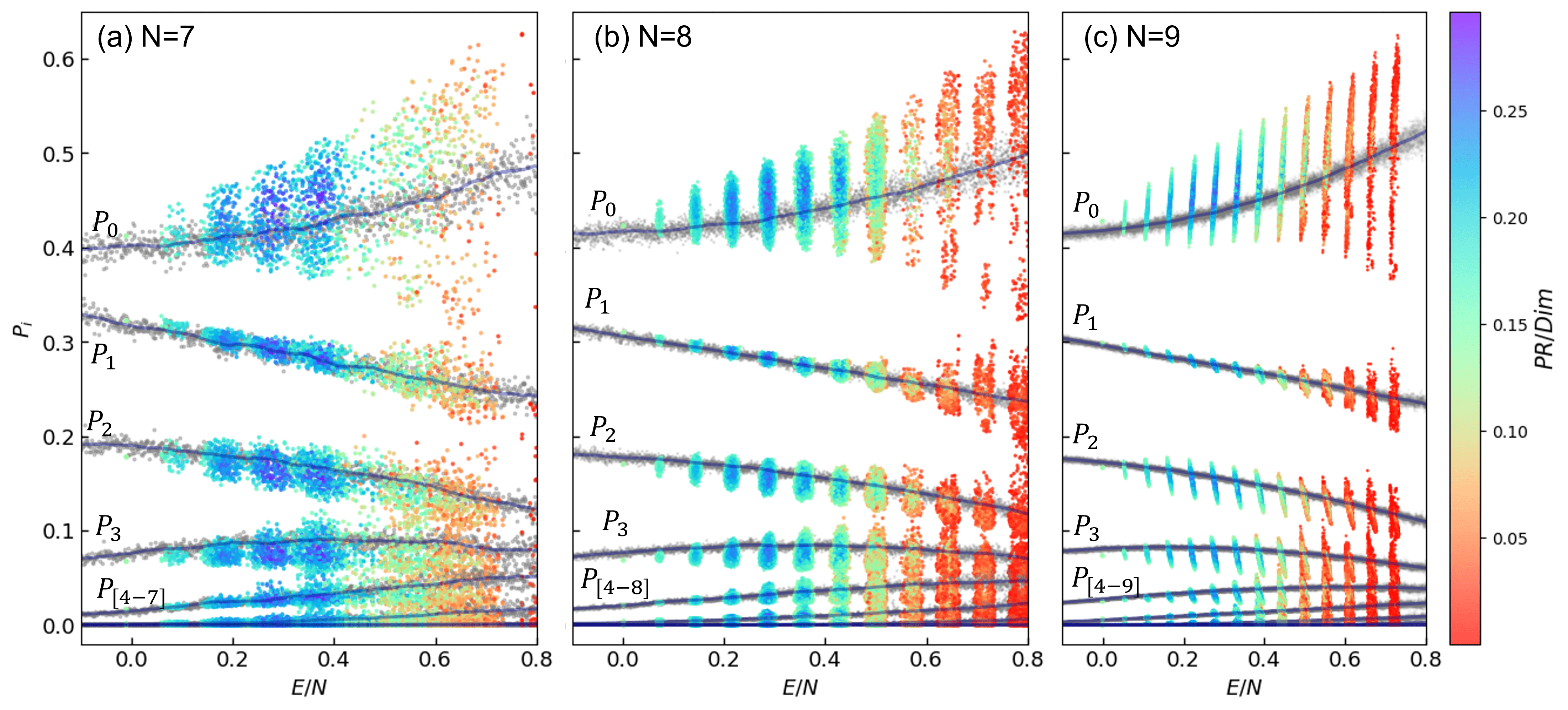
Figure 9: In light gray, eigenstate expectation values for the occupation probabilities of the first site, the dark blue line is the mean value at constant windows of 30 eigenstates (microcanonical average). Coloured dots are the equilibrium values ($t\approx 10^{4}$) of the occupation probabilities of the first site for initial occupation states. Colour scale represent the quotient between participation ratio (PR) of the occupation states in the energy eigenbasis and the dimension of the Hilbert space.

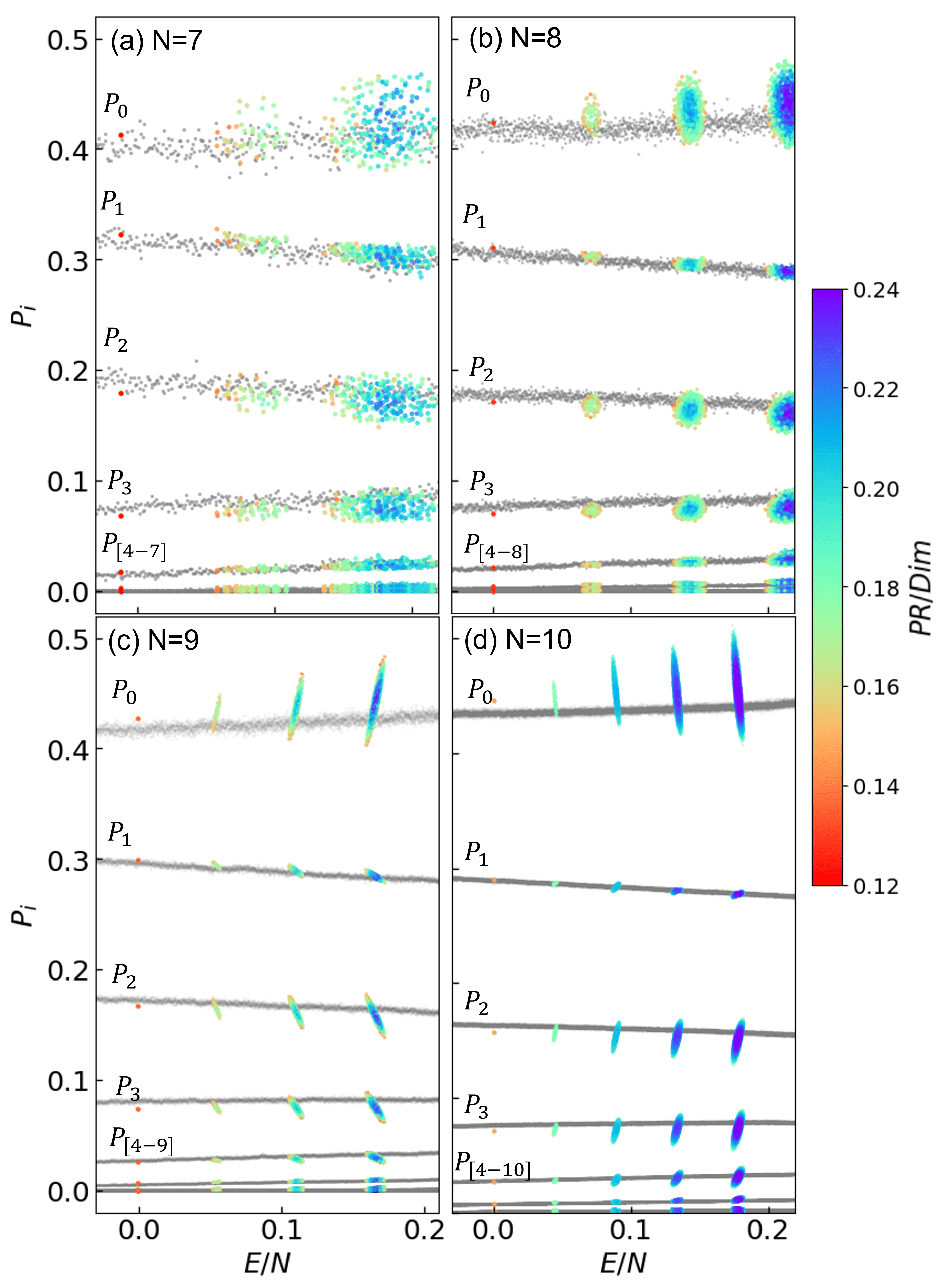
Figure 10: Same as Fig.9 for a shorter energy interval $E/N\in[0,0.2]$, considering four different system sizes $N=M=7,8,9$ and $10$.

Figures 9 and 10 illustrate a comparison between the equilibrium values of the occupation probabilities of the first site $P_{i}$ and the values obtained from the eigenstates. The Participation Ratio (PR) of the occupation states are depicted using a color code, while the microcanonical average is presented in Fig. 9 by a continuous dark blue line. It is evident that the equilibrium values organize in several clusters, each with a number of states that increases as energy does. The clusters are associated to different numbers of the crowding parameter. The leftmost cluster formed by a sole point correspond to $C=1$ and is constituted by the Mott state (an initial atom in each site). Notably, the clusters of lower energies exhibit occupation probabilities that closely align with the microcanonical average. As the energy is increased, the clusters show larger dispersions, though in a different rate depending on the considered $P_{i}$. For example, $P_{1}$ exhibits dispersion of values much smaller than the other probabilities. Observe that the clusters of $P_{1}$ align perfectly to the eigenstates probabilities for the energy range shown in Fig. 10, for the four different sizes considered there. The figures 9 and 10 highlight that the relaxation values of certain initial occupation states deviate from the microcanonical average. The dispersion of values increases as a function of the crowding parameter (and energy), and within each cluster the states with lower PR present larger deviations.

While Fig. 9 allows to observe the occupation probabilities of the first site for a wide energy for $N=M=7,8,9$, Fig. 10 presents a more detailed view in the energy range $E/N\in[0.0,0.2]$, including results for $N=M=10$. It is possible to observe that the centroids of the colored clusters, depicting the equilibrium values of the occupation probabilities of the first site for long time evolution of states in the occupation basis, are slightly displaced from the gray slim line showing the occupation probabilities of the eigenstates.

We examine now the equilibration values of the same observables we have already studied in the previous section for the eigenstates: the number of particles and the entanglement entropy of the first site.

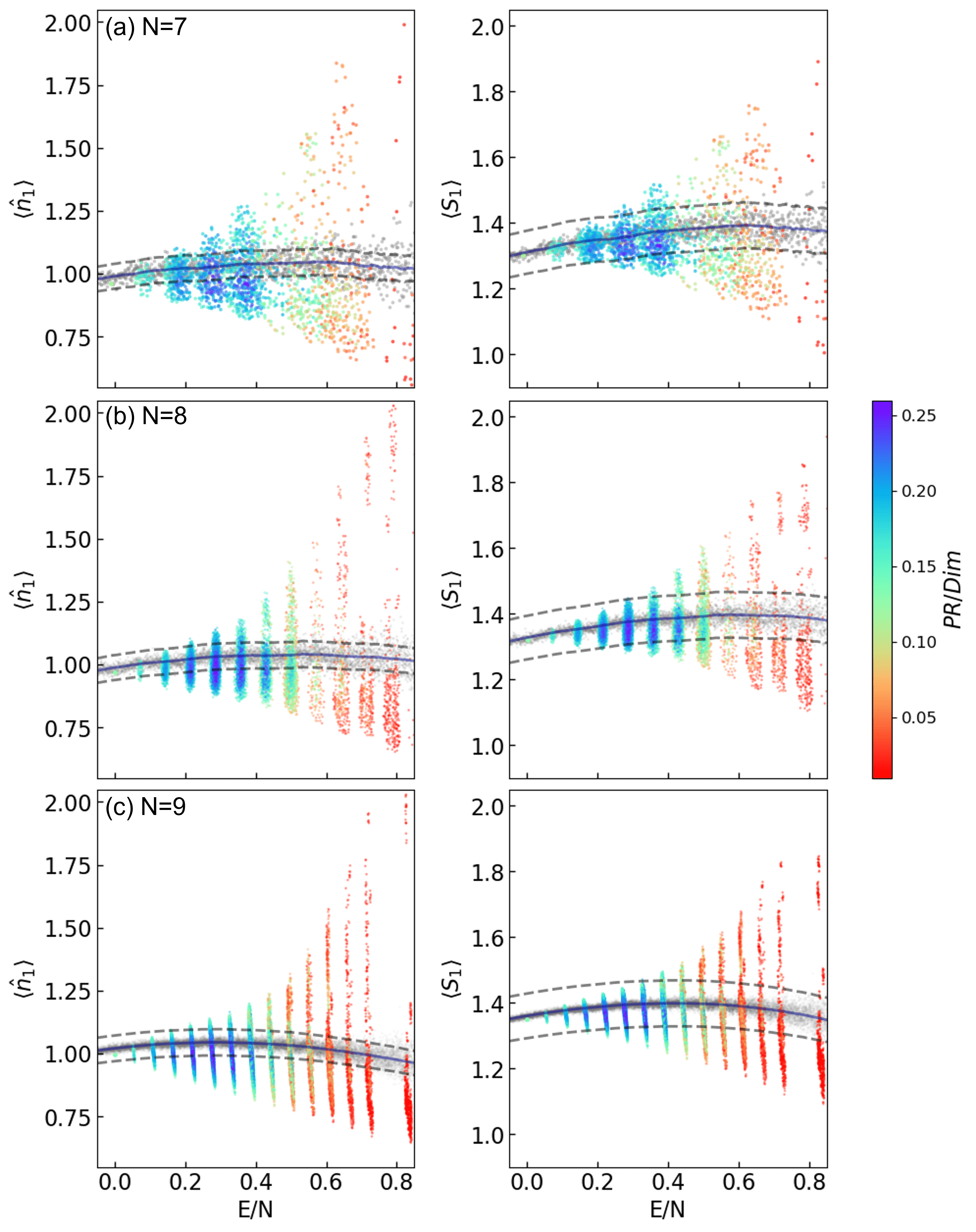
Figure 11: Relaxation values ($t\approx 10^{4}$) of initial states in the occupation basis for the atomic occupation number of the first site (left column) and the entanglement entropy of the first site (right column). Each row represents different number of bosons, (a) $N=M=7$, (b) $N=M=8$ and (c) $N=M=9$. In the background is shown in gray dots the eigenstate expectation value for both observables, the blue line represents the microcanonical average. Gray dashed lines represent deviations of $10\%$ respect to the microcanonical value. All graphs are displayed with a color map representing the averaged PR/Dim of the occupation states respect to the energy eigenbasis.

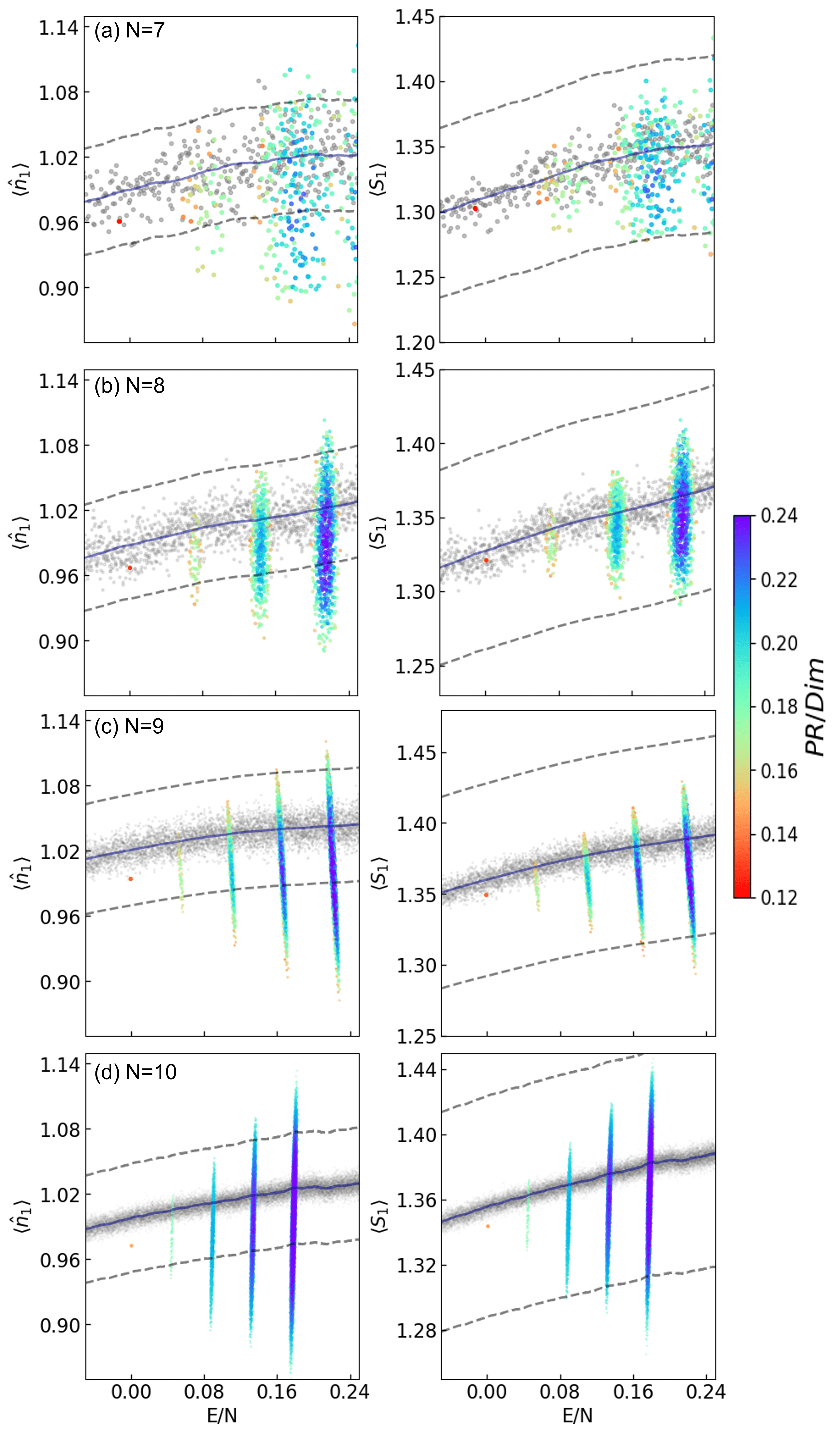
Figure 12: Same as Fig.11 for a shorter energy interval and including four different system sizes: (a) $N=M=7$, (b) $N=M=8$, (c) $N=M=9$, and (d) $N=M=10$.

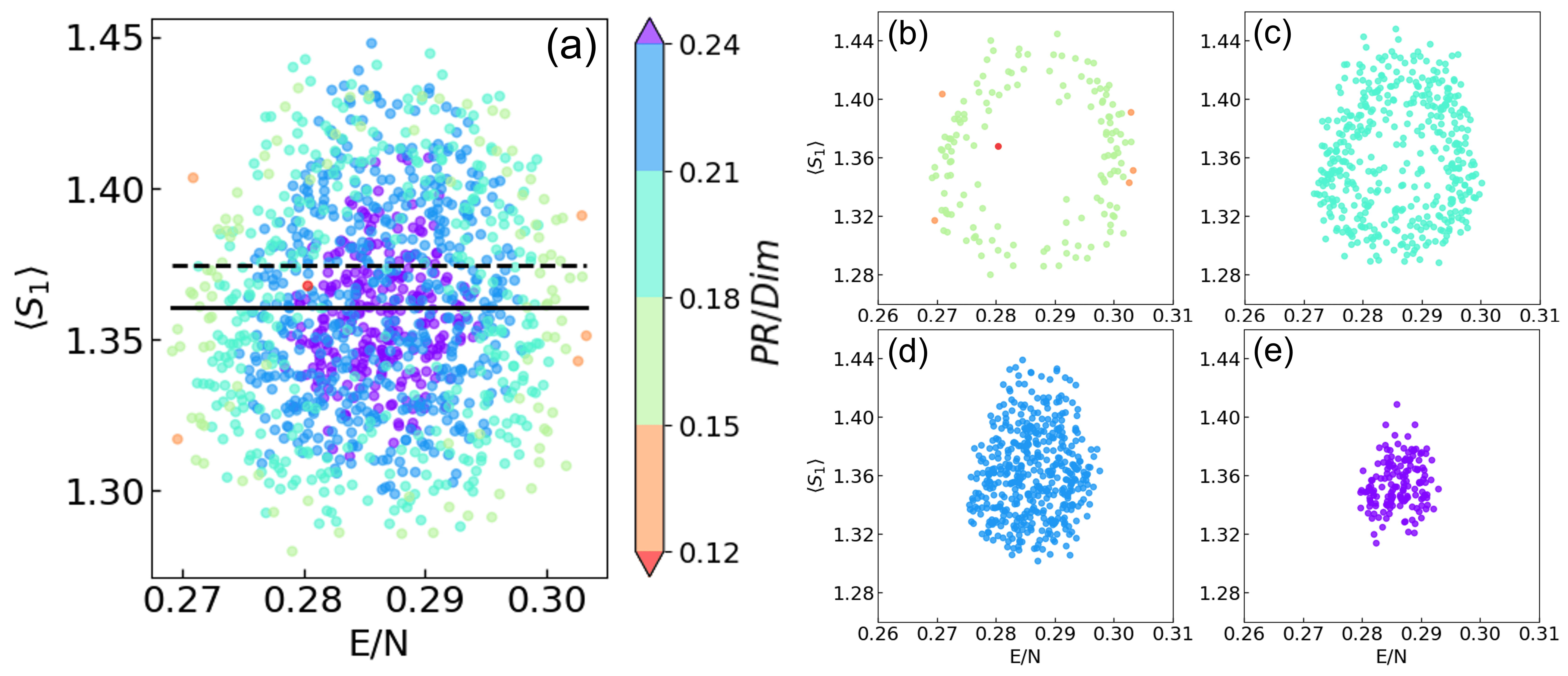
Figure 13: (a) $S_{1}$ vs $E$ colored by the PR for all the occupation states with crowding parameter $C=2$. System size is $N=M=8$. The dashed line is the microcanonical average in the region $C=2$ and the solid black line is the average of all these occupation states. (b)-(e) Same graphic as (a), but separated according to their respective PR values

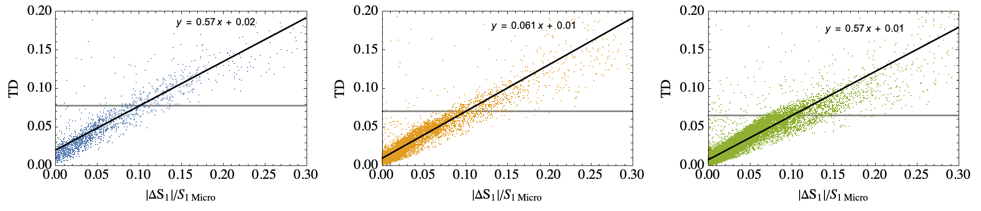
Figure 14: TD is plotted against $\Delta S/S_{1\text{micro}}$ for three different system sizes: left $N=M=7$, middle $N=M=8$ and right is for $N=M=9$. The correlation between these two observables closely resembles a linear relationship. The continuous black line represents the linear fit to the data, and the gray line indicates the value corresponding to $\Delta S/S_{1\text{micro}}=0.1$, which corresponds to a 10% difference between the microcanonical entropy and the occupation states entropy.

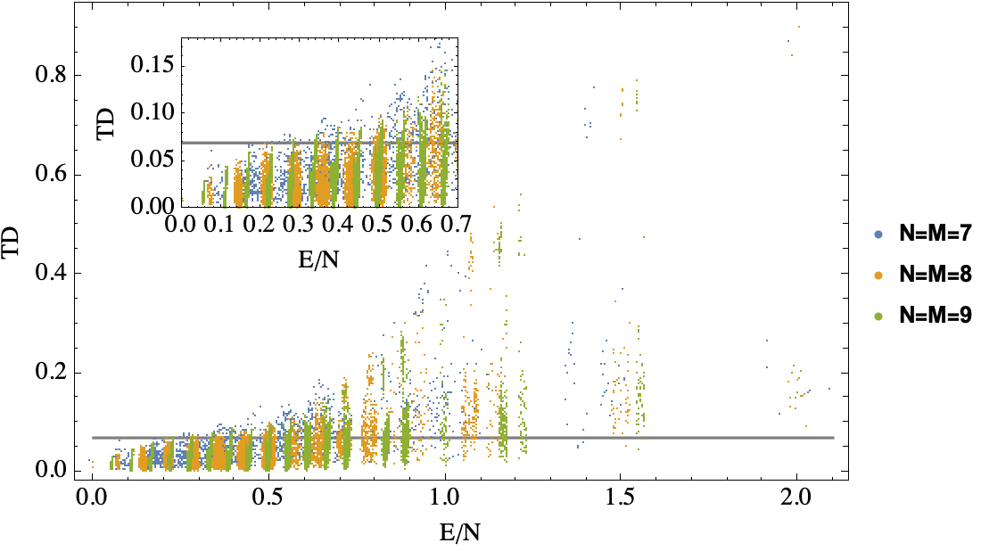
Figure 15: The figure depicts the trace distance between the microcanonical ensemble and the number states evolved at $t=10^{4}$ as a function of the expectation value of the occupation states for three different system sizes.

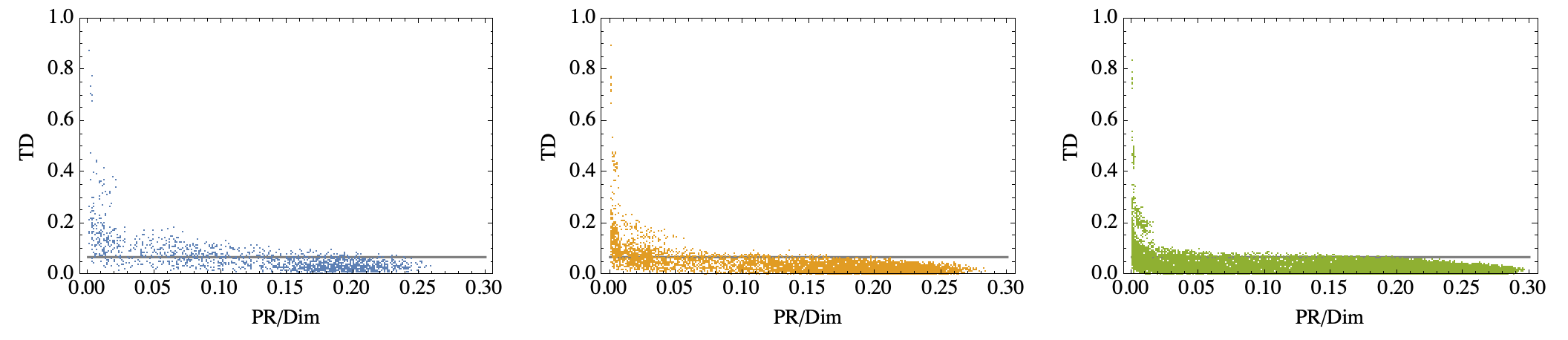
Figure 16: Trace distance (TD) of the microcanonical ensemble and the equilibrium reduced density matrix of initial occupation states versus the energy participation ratio (PR) of the occupation states respect to the energy eigenbasis. Thre different system sizes are considered: $N=M=7$ (left), $N=M=8$ (middle) and $N=M=9$ (right). States with low PR exhibit high TD values, while states with high PR tend to have lower TD values.

A comprehensive picture of the behaviour of the relaxation values of the two observables $n_{1}^{(q)}$ and $S_{1}^{(q)}$ is obtained by plotting their average over 40 Hamiltonian realizations for the whole set of initial states in the occupation basis. These values for initial states having energies in the chaotic energy region $E/N\in[0,0.8]$ are depicted in Fig.11 for three different systems sizes $N=M=7,8$ and $9$. The relaxation values are shown in a rainbow scale according to the PR values of the initial states. The ensemble averages of the observables for the energy eigenstates are shown by gray dots in the background.

Similar to the occupation probabilities, the relaxation values get organized in several clusters associated each to a value of the crowding parameter. Begining in $C=1$, from left to right the crowding parameter increases and so does the mean energy of the states. The relaxation value of the Mott state ($C=1$) in all panels is close to the values coming from the energy eigenstates, i.e., the ETH is satisfied for this state. This initial state was the one extensively studied experimentally in Ref. [5]. As we move to states with higher energies, the ETH is not perfectly satisfied for some states, but the relaxation values in each cluster are located around the trend given by the ensemble averages for eigenstates. The microcanonical average, Eq. (11), and deviations of ten percent around it are shown in the figure by solid and dashed lines, respectively.

The dispersion of the relaxation values in each cluster increases as energy does, but states with high PR present a lower dispersion and concentrate in the inner part of the cluster, whereas states with low PR sit in a much ampler region of the respective cluster, thus having a larger dispersion in their equilibration values. These properties can be more clearly seen in Fig. 12, where a closer view to the first clusters is presented. The cluster structure is clearly seen for the system sizes considered, $N=M=7,8,9,$ and now including $N=M=10$. Unexpectedly, the Mott state show a slight downward deviation respect to the eigenstates averages as the system size is increased. For other clusters in the energy range shown, a similar downward deviation is observed respect to the eigenstates averages.

We can analyze how high and low PR states behave into each cluster. For that purpose we present in Fig. 13 the behaviour of the entanglement entropy for the cluster with crowding parameter $C=2$ in the case $N=M=8$ (similar patterns are found into the other clusters). In panel (a) we plot the relaxation values of $S_{1}$ for all initial states belonging to the cluster versus their average energy. The color of the points indicate their PR. We can see clearly the trend: states with higher participation ratio tend to localize at the center of the cluster, while states with lower PR spread in wider intervals of $S_{1}$ and $E$. The cluster of relaxation values is not centered around the microcanonical value (dashed line) but is slightly shifted downwards. That is why the mean value of the $S_{1}$ in the cluster (solid line) is below the microcanonical value. Panels (b)-(d) in the same Fig. 13, make evident that states with high $PR$ [panels (d) and (e)] locate in the center of the cluster, whereas states with low PR [panels (a) and (b)] locate in the outer borders of the cluster, avoiding the center of the cluster and forming rings.

IV.2 Quantifying the lack of thermalization.

From the results of previous subsection, it is clear that relaxation values of low PR states in the occupation basis tend to deviate more respect to the thermal averages than states with high PR. In this subsection, we determine if these deviations are significative.

In order to quantify the thermal deviation of the equilibirum state that is attained by initial states in the occupation basis, we consider 1) the relative deviation of the entanglement entropy of the first site respect to the thermal average and 2) the trace distance between the microcanonical density matrix in the first site $\rho_{A}^{mc}$ and the reduced density matrix in the first site of the state evolved unitarily from an initial state in the occupation basis $\rho_{A}$. We define both quantities in the following.

The relative deviation of the entanglement entropy respect to the thermal value is

$$\frac{|\Delta S_{1}|}{S_{1\text{micro}}}=\frac{|S_{1}-S_{1\text{micro}}|}{S_{1\text{micro}}},$$ (12)

where $S_{1\text{micro}}$ is the entropy value at the first site in the microcanonical ensemble, Eq. 11, and $S_{1}$ is the equilibrium value of the entropy of each occupation state.

The Trace Distance (TD) of two reduced density matrices, on the other hand, is

$$\text{TD}=\frac{1}{2}\text{Tr}\left|\rho_{A}^{\text{mc}}-\rho_{A}\right|,$$ (13)

where $\rho_{A}^{\text{mc}}$ is the microcanonical density matrix in the first site and $\rho_{A}$ is the reduced density matrix in the first site of the state evolved unitarily from an initial state in the occupation basis. Along this work we employ observables related with only one site. In this case, the trace distance takes the simple form

$$\text{TD}(q)=\frac{1}{2}\sum_{i}^{M}\left|p_{i,\text{micro}}-p_{i}^{(q)}\right|.$$ (14)

When TD is close to zero, the two matrices are similar, and we say that the system thermalizes. Conversely, if TD is close to one, we say that the system does not thermalize. In the following, we determine a reference value of TD allowing us to distinguish between thermal and non-thermal states.

In Fig.14 we show the trace distance plotted versus the relative deviation of the entropy for all the initial states in the occupation basis, for $N=M=7,8$ and $9$. The Figure shows that, as it could be expected, both quantities are related in a simple way. For the three system sizes considered, a linear relation is obtained TD $\propto|\Delta S_{1}|/S_{1\text{micro}}$. From these results, we obtain that thermal deviations of equilibration values less than $10\%$ correspond to TD$<0.07$. Therefore, this latter value can be used as a reference to establish if a equilibrium state thermalize (TD$<0.07$) or not (TD$>0.07$). It is worth emphasizing that the trace distance depends exclusively on the states, and therefore guarantees thermalization for any observable.

In Figs. 15 and 16, we observe the behavior of the equilibrium TD for the initial states in the occupation basis. In Fig. 15, for three different system sizes, we show the TD for all the occupation states as function of their respective energy. We observe that for states with $E/N<0.6$, most of the TD values are less than 0.07, indicating that most of these states thermalize. For higher energy values, a larger fraction of states do not thermalize. It is important to note that for all system dimensions, the value $E/N\approx 0.6$ marks the point where a proliferation of non-thermalizing states begin to appear, in close correspondence with the transition from chaos to regularity in the spectrum shown in Fig.1.

Fig. 16 shows the TD but now as a function of the PR/Dim of all the states in the occupation basis, for three different system sizes. It is observed that states with high PR/Dim>$0.20=1/5$ have a trace distance below TD $<0.07$, indicating that they thermalize. As the value of PR/Dim decreases a larger fraction of states have TD values above $0.07$, i.e. the fraction of non-thermal states increases. It can be concluded that a PR larger than Dim/5 is a sufficient condition for thermalization, but there are many states with smaller PR which can also be described as thermalized under the present criteria.

V Conclusions

A meticulous spectral analysis of the Aubry-André model has been conducted, utilizing averages derived from 40 numerical diagonalizations and random $\phi$ samplings within the $[0,2\pi]$ range. The findings provide compelling evidence of thermalization within the chaotic system’s eigenstates, as demonstrated by the smooth dependence of average occupation and entanglement entropy on energy. The adherence to the Eigenstate Thermalization Hypothesis (ETH) is further supported by the inverse relationship of the standard deviation, and the discrepancy between maximum and minimum values, of entanglement entropy and particle number at the first site, with the size of the system.

Comparisons of observable values with the microcanonical average highlight the presence of occupation states deviating from this average, particularly among states with low participation ratios in the energy eigenbasis. These discoveries underscore the validity of ETH within the Aubry-André model, offering insights into the underlying mechanisms governing thermalization in disordered quantum systems.

In this study we considered a linear chain with open boundary conditions. It would be intriguing to explore whether the dispersions of equilibrium values observed here would diminish in the case of a chain with periodic boundary conditions.

- [1] Thilo Stöferle, Henning Moritz, Christian Schori, Michael Köhl, and Tilman Esslinger. Transition from a strongly interacting 1d superfluid to a mott insulator. Phys. Rev. Lett., 92:130403, Mar 2004.
- [2] L. Fallani, J. E. Lye, V. Guarrera, C. Fort, and M. Inguscio. Ultracold atoms in a disordered crystal of light: Towards a bose glass. Phys. Rev. Lett., 98:130404, Mar 2007.
- [3] G. Roux, T. Barthel, I. P. McCulloch, C. Kollath, U. Schollwöck, and T. Giamarchi. Quasiperiodic bose-hubbard model and localization in one-dimensional cold atomic gases. Phys. Rev. A, 78:023628, Aug 2008.
- [4] Adam M Kaufman, M Eric Tai, Alexander Lukin, Matthew Rispoli, Robert Schittko, Philipp M Preiss, and Markus Greiner. Quantum thermalization through entanglement in an isolated many-body system. Science, 353(6301):794–800, 2016.
- [5] Alexander Lukin, Matthew Rispoli, Robert Schittko, M. Eric Tai, Adam M. Kaufman, Soonwon Choi, Vedika Khemani, Julian Léonard, and Markus Greiner. Probing entanglement in a many-body-localized system. Science, 364(6437):256–260, 2019.
- [6] Markus Greiner, Olaf Mandel, Tilman Esslinger, Theodor W. Hänsch, and Immanuel Bloch. Quantum phase transition from a superfluid to a mott insulator in a gas of ultracold atoms. Nature, 415(6867):39–44, 2002.
- [7] Immanuel Bloch, Jean Dalibard, and Wilhelm Zwerger. Many-body physics with ultracold gases. Rev. Mod. Phys., 80:885–964, Jul 2008.
- [8] Manuel Endres, Hannes Bernien, Alexander Keesling, Harry Levine, Eric R. Anschuetz, Alexandre Krajenbrink, Crystal Senko, Vladan Vuletic, Markus Greiner, and Mikhail D. Lukin. Atom-by-atom assembly of defect-free one-dimensional cold atom arrays. Science, 354(6315):1024–1027, 2016.
- [9] G. Roux, T. Barthel, I. P. McCulloch, C. Kollath, U. Schollwöck, and T. Giamarchi. Quasiperiodic bose-hubbard model and localization in one-dimensional cold atomic gases. Phys. Rev. A, 78:023628, Aug 2008.
- [10] Rubem Mondaini and Marcos Rigol. Many-body localization and thermalization in disordered hubbard chains. Phys. Rev. A, 92:041601, Oct 2015.
- [11] J. M. Deutsch. Quantum statistical mechanics in a closed system. Phys. Rev. A, 43:2046–2049, Feb 1991.
- [12] Mark Srednicki. Chaos and quantum thermalization. Phys. Rev. E, 50:888–901, Aug 1994.
- [13] Marcos Rigol, Vanja Dunjko, and Maxim Olshanii. Thermalization and its mechanism for generic isolated quantum systems. Nature, 452(7189):854–858, 2008.
- [14] J M Zhang and R X Dong. Exact diagonalization: the bose–hubbard model as an example. European Journal of Physics, 31(3):591–602, apr 2010.
- [15] A. R Kolovsky and A Buchleitner. Quantum chaos in the bose-hubbard model. Europhysics Letters (EPL), 68(5):632–638, dec 2004.
- [16] Corinna Kollath, Guillaume Roux, Giulio Biroli, and Andreas M Läuchli. Statistical properties of the spectrum of the extended bose–hubbard model. Journal of Statistical Mechanics: Theory and Experiment, 2010(08):P08011, aug 2010.
- [17] Javier de la Cruz, Sergio Lerma-Hernández, and Jorge G. Hirsch. Quantum chaos in a system with high degree of symmetries. Phys. Rev. E, 102:032208, Sep 2020.
- [18] Carlos Diaz-Mejia, Javier de la Cruz, Sergio Lerma-Hernández, and Jorge G. Hirsch. Persistent revivals in a system of trapped bosonic atoms. Physics Letters A, 493:129262, 2024.
- [19] Hans-Jürgen Stöckmann. Quantum chaos: an introduction, 2000.
- [20] Vadim Oganesyan and David A. Huse. Localization of interacting fermions at high temperature. Phys. Rev. B, 75:155111, Apr 2007.
- [21] N.D. Chavda, H.N. Deota, and V.K.B. Kota. Poisson to goe transition in the distribution of the ratio of consecutive level spacings. Physics Letters A, 378(41):3012–3017, 2014.
- [22] Eduardo Jonathan Torres-Herrera and Lea F. Santos. Dynamical detection of level repulsion in the one-particle aubry-andré model. Condensed Matter, 5(1), 2020.
- [23] Y. Y. Atas, E. Bogomolny, O. Giraud, and G. Roux. Distribution of the ratio of consecutive level spacings in random matrix ensembles. Phys. Rev. Lett., 110:084101, Feb 2013.
- [24] Shashi C L Srivastava, Arul Lakshminarayan, Steven Tomsovic, and Arnd Bäcker. Ordered level spacing probability densities. Journal of Physics A: Mathematical and Theoretical, 52(2):025101, dec 2018.
- [25] Marcos Rigol and Lea F. Santos. Quantum chaos and thermalization in gapped systems. Phys. Rev. A, 82:011604, Jul 2010.
- [26] Anatoli Polkovnikov Luca D’Alessio, Yariv Kafri and Marcos Rigol. From quantum chaos and eigenstate thermalization to statistical mechanics and thermodynamics. Advances in Physics, 65(3):239–362, 2016.