Universal Scaling Laws for a Generic Swimmer Model
Abstract
We have developed a minimal model of a swimmer without body deformation based on force and torque dipoles which allows accurate 3D Navier-Stokes calculations. Our model can reproduce swimmer propulsion for a large range of Reynolds numbers, and generate wake vortices in the inertial regime, reminiscent of the flow generated by the flapping tails of real fish. We performed a numerical exploration of the model from low to high Reynolds numbers and obtained universal laws using scaling arguments. We collected data from a wide variety of micro-organisms, thereby extending the experimental data presented in (M. Gazzola et al., Nature Physics 10, 758, 2014). Our theoretical scaling laws compare very well with experimental data across the different regimes, from Stokes to turbulent flows. We believe that this model, due to its relatively simple design, will be very useful for obtaining numerical simulations of collective effects within fish schools composed of hundreds of individuals.
Introduction The wide variety of means employed by living creatures to move in aquatic environments is fascinating Childress (1981). Motion generally involves a complex interplay between the deformation of the body and the surrounding fluid. From the smallest organisms, like bacteria, to colossal blue whales Berg (2004); S.Powar et al. (2022); Garcia et al. (2011); Smits (2019); Gray (1936); Wolfgang et al. (1999); Dabiri et al. (2006); Müller et al. (2001), the differences in length scale , velocity and mode of locomotion are so vast that the elaboration of a universal model to describe swimming across these scales might seem impossible.
The importance of inertia with respect to viscous dissipation is quantified by the Reynolds number, which expresses the ratio of stress due to inertia to stress due to viscosity: , where and represent fluid density and viscosity, respectively. The Reynolds numbers associated with aquatic living species span several decades, typically ranging from for fish to for micro-organisms like spermatozoa. Consequently, the drag force exerted by the fluid on the swimmer is largely dependent on the species considered, originating from either fully viscous dissipation at the small scale, or turbulent inertia at the large scale.
As a result, each swimming model Taylor (1951); Spagnolie and Lauga (2010); Lauga (2020); Lighthill (1960); Liu and Kawachi (1999); Kern and Koumoutsakos (2006) tends to offer a tailored approach specific to the flow regime considered and the corresponding body deformation. Most models focus on periodic body deformation, coupled with the surrounding fluid, and resolve the full swimming cycle. This provides specific approaches that address swimming at small scales, where viscous forces dominate (e.g. for micro-organisms Lauga and Powers (2009)), differently from the macroscopic strategies of large fish or mammals, which can leverage the inertia of the surrounding fluid to break time reversibility Purcell (1977). The highly diverse physical origins of particular swimming patterns represent an obstacle to the exploration of a more comprehensive and universal viewpoint.
In this letter, we propose a different approach. Deformation kinematics, such as undulations, oscillations and pulsations, are ignored, and locomotion is described using force and torque dipoles applied by a solid body of finite size on a fluid. While a similar description has already been used for micro-swimmers at low Hernandez et al. (2005); Mehandia and Nott (2008); Jibuti et al. (2014), to the best of our knowledge, it has never yet been employed for high , when inertia starts to dominate viscous forces. In this work, we study the motion described by our model over decades of Reynolds numbers (), theoretically and numerically, comparing our results with experimental data. Although the direct effect on swimming velocity of the specific deformation of the swimmer’s body is acknowledged, particularly as it can reduce the drag force Gray (1936); Li et al. (2021), we would like to emphasize that we are not attempting to provide a detailed and precise analysis of a particular mode of locomotion, but rather a more universal description in terms of the forces applied to the fluid. While our swimmer model is minimal, the motion of the surrounding fluid is accurately captured using the full numerical resolution of the 3D Navier-Stokes equation, and our approach encompasses the different swimming regimes of a wide variety of aquatic species. Our model can also remarkably reproduce the characteristic wake vortices observed behind fish due to the flapping of their tails Drucker and Lauder (2002).
Our approach furthermore exhibits universal scaling laws which link the swimming Reynolds number to a new dimensionless group, the thrust number defined below. We identify three different regimes: the Stokes regime (), a laminar regime () and a turbulent regime (), and calculate the theoretical exponents of the scaling laws in the three regimes using simple scaling analyses (independently of the space dimension). These compare very well with the numerical simulations produced by our generic swimmer model. We also validate our results with experimental data presented in Gazzola et al. (2014) for the laminar and turbulent regimes, and further extend this validation with data collected on micro-swimmers for the Stokes regime.
Swimmer model.
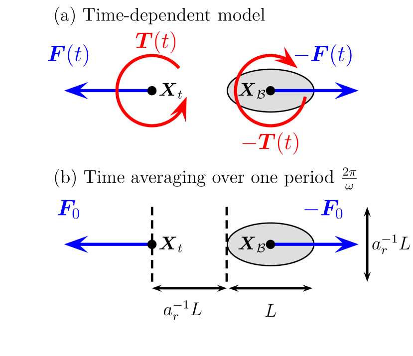
The model uses a time-dependent force dipole combined with a torque dipole (Fig. 1(a)), both attached to a rigid body of ellipsoidal shape. An autonomous swimming body creates its own motion, therefore the total sum of forces and torques must cancel out, due to the third law of Newton of the fluid-body system. Feynman et al. (2006). The model developed by Filella et al. (2018) presents some conceptual similarities. It represents each fish as a point-like active particle bearing a dipole in a potential 2D inviscid fluid, which allows consideration of the hydrodynamic interactions between fish in the far-field limit. However, since our aim is to explore a wide spectrum of Reynolds numbers (from viscous to inertial regimes), we solved the full incompressible Navier-Stokes equations in 3D and 2D (see SM ven (a)).
The swimmer exerts on the fluid a force dipole like that generally used for a micro-swimmer at a low Hernandez et al. (2005); Mehandia and Nott (2008); Jibuti et al. (2014) (see Fig. 1). We used a pusher-like model that reproduces the force distribution of a fish at high Reynolds numbers. This approach can easily be extended to a more detailed model by using more complex force distributions (e.g. Mehandia and Nott (2008)). As shown in Fig. 1(a), the force dipole is composed of one force applied in the fluid at the rear of the body , mimicking a swimming organ, and an opposite force exerted inside the body at the center-of-mass . The force is time-dependent with pulsation and pusher-like: with . The absolute value in the expression of enforces the pusher nature of the swimmer. We also consider a torque dipole: , collocated with the force dipole. The torque at the back represents the stroke of the swimming organ and causes the vortex street Drucker and Lauder (2002) in the fish’s wake at high . An opposite torque is applied in the body (Fig. 1(a)), and represents the counter-reaction of the rest of the body. For practical reasons in the scaling analyses below, we also introduce force and torque densities and respectively. Averaging these dipoles over one period of time () results in a simple static force dipole (Fig. 1(b)), while the average torque cancels out. This time averaging over one beating period is very similar to models of pushers and pullers beating at low Hernandez et al. (2005); Mehandia and Nott (2008); Jibuti et al. (2014).
Scaling laws. The hydrodynamic nature of our model allows for simple scaling arguments, inspired by Gazzola et al. (2014) for inertial flows but translated to a more generic framework and extended to the non-inertial Stokes regime. In the following, we present arguments, but they remain valid in (see SM ven (a)). We also consider that all the lengths scale as .
The body of the swimmer is submitted to different dominant drag forces depending on the Reynolds number. To describe this effect across all swimming regimes, we introduce the thrust number as the ratio between the applied force density multiplied by inertial forces , and the square of viscous forces , which gives
| (1) |
The thrust number appears naturally at all scales of Reynolds numbers, as shown below. It contains the force term at the origin of the motion, which is characterized by the Reynolds number. It therefore provides a convenient method for evaluating velocity as a function of force. Let us consider classic scaling arguments:
-
•
At high Reynolds numbers, the boundary layer around the body is turbulent and pressure drag dominates. The corresponding force scales as . Since , we obtain .
-
•
For small but finite Reynolds numbers, the regime is laminar and the viscous force in the boundary layer dominates: where is the thickness of the boundary layer, which obeys the Blasius law Landau and Lifshitz (2013) . This finally leads to .
-
•
At low Reynolds numbers, the Stokes drag force dominates and the force applied on the body compensates the drag: . This gives .
From the Stokes to the turbulent regime, we observe that the exponent of the scaling is always below one and decreases. It suggests a diminishing swimming performance as the Reynolds number of the swimmer increases. To confirm these three successive regimes, we present below numerical simulations with our swimmer model, exploring a large range of values for the thrust and Reynolds numbers.
Numerical simulations.
We performed direct numerical simulations of the incompressible Navier-Stokes equations in the presence of our model swimmer, a rigid ellipsoid body with the force and torque dipoles attached. The corresponding fluid momentum balance equation writes:
| (2) |
where and are respectively the velocity and pressure fields, denotes the material derivative , is the strain-rate tensor, and denote the density and viscosity fields, and and respectively represent the – time-varying – force and torque dipoles attached to the swimmer, as introduced above. The rigid body of the swimmer is accounted for with a fictitious domain penalty method inspired by (Janela et al., 2005); in practice, this can be implemented simply with a spatially-variable viscosity (Tanaka and Araki, 2000): where is the indicator – or Heaviside – function of . In practice, a viscosity ratio is applied between the fluid and the swimmer body to ensure that the rigid motion constraint is satisfied within . Density is defined as constant inside and outside , thus making the swimmer neutrally buoyant. Note that this fictitious domain penalty method allows the swimmer to be treated directly as part of the Navier-Stokes equations through the viscosity field, thereby avoiding the need to deal with moving boundary conditions and potential remeshing issues at the body interface in the discrete setting. The incrompressible Navier-Stokes equations are solved numerically using an implicit finite element method (Metivet et al., 2018) implemented in the parallel FEEL++ library Prud’homme et al. (2012). The position and orientation of the swimmer are updated at each time-step using a first order Euler scheme with the translational and rotational velocities computed from the fluid velocity field in . A comprehensive derivation of the numerical model and technical details are provided in SM ven (a).
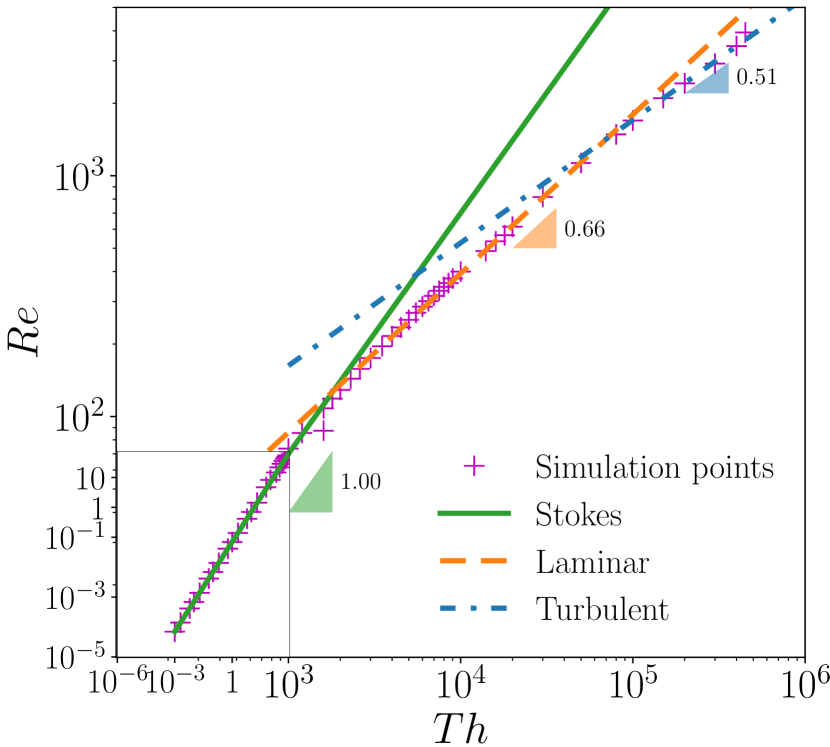
This numerical framework is used to explore a large range of Reynolds numbers () and Thrust numbers (, in order to evaluate the dependence of as a function of while varying each of the model’s different parameters (, , , and ) separately (see SM ven (a)). As shown in Fig. 2, the numerical simulations are in perfect agreement with the scaling laws presented above, displaying the Stokes regime in the range , the laminar regime for and the turbulent regime for ,
with fitting exponents that match the predictions. Note that the ranges of each regime depend on the aspect ratio of the swimmer , which is kept constant. We also found that and do not play any role in the dependency, which confirms that all the important parameters are embedded in the number.
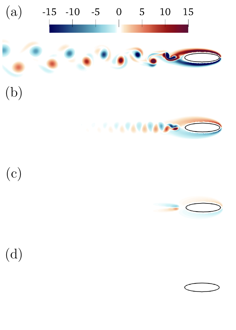
Wake and vortices. Although torque plays no role in the scaling of as a function of , it is essential to reproduce the wake at the rear of the swimmer in the inertial regime. The torque dipole can be used to account for flagellum, body undulation or tail beating to generate a reverse von Karman vortex street, as observed in the wake of a fish at high number Kern and Koumoutsakos (2006); Ko et al. (2023).
Figures 3(a,b) illustrate the typical wakes obtained with in 2D simulations.
The vortices created at the same frequency are spaced further apart as the Reynolds number (i.e. velocity) increases from to . The length over which they dissipate becomes shorter towards the viscous regimes (Fig. 3(c)), vanishing completely at low (Fig. 3(d)). Indeed, no vortices are present behind micro-organisms Drescher et al. (2010).
Comparison with experimental data. To compare our scaling results with experimental data, forces must be expressed in terms of observable data (Fig. 4), such as undulation or tail beating frequency. Although force , torque and pulsation are independent quantities in the model, physical constraints exist between these quantities in living organisms. We made the reasonable assumption that the size of the swimming organ scales with the size of the body Gazzola et al. (2014). Force and torque generated by the swimming organ are such that .
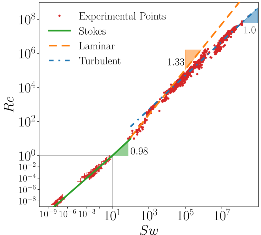
In inertial regimes, i.e. excluding the Stokes regime that we address separately, the instantaneous force creates a transient acceleration of the fluid, which scales with , i.e. . Introducing the observation-based swimming number Gazzola et al. (2014), the theoretical force drive can be related to experimentally measurable data as . The scaling laws previously derived from our model can thus be reformulated in terms of : in the laminar regime , while in the turbulent regime , in accordance with the results of Gazzola et al. (2014).
In the Stokes regime, the force exerted by the swimming organ is balanced by viscous drag, so that . Reintroducing again the swimming number , we obtain , leading to . Note that this is a natural consequence of the absence of inertia: each stroke creates a net displacement that scales with , inducing a swimming velocity .
Figure 4 shows the experimental data collected from micrometer- to meter-size aquatic organisms along with the corresponding fitted scaling laws. In addition to the results from Gazzola et al. (2014), an excellent agreement between experimental data and hydrodynamic scaling laws is also obtained in the Stokes regime.
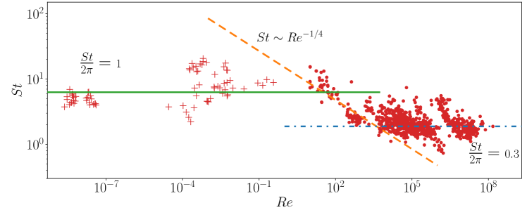
Note that in both the Stokes and turbulent regimes, so that the corresponding Strouhal number is constant, as illustrated in Figure 5. The transition between Gazzola et al. (2014) and occurs in the laminar regime where .
Conclusion. By avoiding direct fluid-structure coupling, our generic swimmer model provides an efficient model for hydrodynamic propulsion, while retaining the salient features of swimming organisms across several decades of Reynolds numbers. High numerical stability and efficiency ensure fully tractable 2D and 3D simulations, thereby paving the way to large scale simulations with hundreds of agents. It also proposes a methodology for progressive refinement of the hydrodynamic field, by retaining higher moments of forces and torques, resulting in more complex propulsion models. This approach broadens our understanding of the swimming of aquatic organisms by revealing the universal relationship between the velocity of a swimmer and the force exerted by its swimming organ. The sub-linear dependence demonstrated between and suggests diminishing swimming performance as the swimmer’s Reynolds number increases. The scaling laws obtained also match the experimental data obtained from thousands of aquatic animals, ranging from large mammalians to micro-organisms. Our results shed new light on the general mechanisms underlying swimming and provide an efficient and robust numerical framework to investigate the collective behavior of swimmers in complex environments.
Acknowledgements. This project received financial support from the French National Research Agency (ANR-21-CE45-0005, FISHSIF project).
References
- Childress (1981) S. Childress, Mechanics of Swimming and Flying (Cambridge University Press, 1981).
- Berg (2004) H. Berg, E.coli in motion (Springer, 2004).
- S.Powar et al. (2022) S.Powar, F. Parast, A. Nandagiri, A. Gaikwad, D. Potter, M. O’Bryan, R. Prabhakar, J. Soria, and R. Nosrati, Small Methods 6, e2101089 (2022).
- Garcia et al. (2011) M. Garcia, S. Berti, P. Peyla, and S. Rafaï, Phys. Rev. E 83, 035301 (2011).
- Smits (2019) A. Smits, J. Fluid. Mech., Perspectives 874, 1 (2019).
- Gray (1936) J. Gray, J. Exp. Biol. 13, 192 (1936).
- Wolfgang et al. (1999) M. Wolfgang, J. Anderson, M. Grosenbaugh, D. Yue, and M. Triantafyllou, J. Exp. Biol. 202, 4841 (1999).
- Dabiri et al. (2006) J. O. Dabiri, S. P. Colin, and J. H. Costello, J. Exp. Biol. 209, 17 (2006).
- Müller et al. (2001) U. Müller, J. Smit, E. Stamhuis, and J. Videler, J. Exp. Biol. 204, 2751 (2001).
- Taylor (1951) G. I. Taylor, Proc. R. Soc. Lond. A 209, 447 (1951).
- Spagnolie and Lauga (2010) S. Spagnolie and E. Lauga, Phys. of Fluids 22, 031901 (2010).
- Lauga (2020) E. Lauga, Phys. Rev. Fluids 5, 123101 (2020).
- Lighthill (1960) M. J. Lighthill, J. Fluid Mech. 9, 305 (1960).
- Liu and Kawachi (1999) H. Liu and K. Kawachi, J. Comp. Phys. 155, 223 (1999).
- Kern and Koumoutsakos (2006) S. Kern and P. Koumoutsakos, J. Exp. Biol. 209, 4841 (2006).
- Lauga and Powers (2009) E. Lauga and T. R. Powers, Reports on Progess in Physics 72, 096601 (2009).
- Purcell (1977) E. Purcell, American Journal of Physics 3–11, 1 (1977).
- Hernandez et al. (2005) J. Hernandez, C. Stoltz, and M. Graham, Phys. Rev. Lett. 95, 204501 (2005).
- Mehandia and Nott (2008) V. Mehandia and P. Nott, J. Fluid Mech. 595, 239 (2008).
- Jibuti et al. (2014) L. Jibuti, L. Qi, C. Misbah, W. Zimmermann, S. Rafaï, and P. Peyla, Phys. Rev. E 90, 063019 (2014).
- Li et al. (2021) G. Li, H. Liu, U. Müller, C. Voesenek, and J. van Leeuwen, Proc. Royal Soc. 288, 1 (2021).
- Drucker and Lauder (2002) E. G. Drucker and G. V. Lauder, Integrative and Comparative Biology 42, 243 (2002), https://academic.oup.com/icb/article-pdf/42/2/243/1841427/i1540-7063-042-02-0243.pdf .
- Gazzola et al. (2014) M. Gazzola, M. Argentina, and L. Mahadevan, Nature Physics 10, 758 (2014).
- Feynman et al. (2006) R. Feynman, R. Leighton, and M. Sands, The Feynman Lectures on Physics, Vol. 1 (Addison-Wesley, 2006).
- Filella et al. (2018) A. Filella, F. Nadal, C. Sire, E. Kanso, and C. Eloy, Phys. Rev. Lett. 120, 198101 (2018).
- ven (a) “See supplementary material at [to-be-inserted-by-publisher],” (a).
- Landau and Lifshitz (2013) L. D. Landau and E. M. Lifshitz, Fluid mechanics: course of theoretical physics, Vol. 6 (Elsevier, 2013).
- Janela et al. (2005) J. Janela, A. Lefebvre, and B. Maury, in ESAIM: Proceedings, Vol. 14 (EDP Sciences, 2005) pp. 115–123.
- Tanaka and Araki (2000) H. Tanaka and T. Araki, Phys. Rev. Lett. 85, 1338 (2000).
- Metivet et al. (2018) T. Metivet, V. Chabannes, M. Ismail, and C. Prud’homme, Mathematics 6, 203 (2018).
- Prud’homme et al. (2012) C. Prud’homme, V. Chabannes, V. Doyeux, M. Ismail, A. Samake, and G. Pena, ESAIM: Proc. 38, 429 (2012).
- Ko et al. (2023) H. Ko, G. Lauder, and R. Nagpal, J. R. Soc. Interface 20, 1 (2023).
- ven (b) “Doi will be added after the peer review,” (b).
- Drescher et al. (2010) K. Drescher, R. E. Goldstein, N. Michel, M. Polin, and I. Tuval, Phys. Rev. Lett. 105, 168101 (2010).