Unwinding Toxic Flow with Partial Information

Abstract

We consider a central trading desk which aggregates the inflow of clients’ orders with unobserved toxicity, i.e. persistent adverse directionality. The desk chooses either to internalise the inflow or externalise it to the market in a cost effective manner. In this model, externalising the order flow creates both price impact costs and an additional market feedback reaction for the inflow of trades. The desk’s objective is to maximise the daily trading P&L subject to end of the day inventory penalization. We formulate this setting as a partially observable stochastic control problem and solve it in two steps. First, we derive the filtered dynamics of the inventory and toxicity, projected to the observed filtration, which turns the stochastic control problem into a fully observed problem. Then we use a variational approach in order to derive the unique optimal trading strategy. We illustrate our results for various scenarios in which the desk is facing momentum and mean-reverting toxicity. Our implementation shows that the P&L performance gap between the partially observable problem and the full information case are of order $0.01\%$ in all tested scenarios.

Mathematics Subject Classification (2010):

91G10, 49N10, 49N90, 93E20, 93E11, 60G35

JEL Classification:

C61, C73, G11, G24, G32,

Keywords:

central risk book, market making, optimal liquidation, price impact, partially observable stochastic control

1 Introduction

The common market situation where buyers and sellers have different information has played a central role in understanding and modeling financial ecosystems. In particular models of informed traders have been at the core of financial research ever since the pioneering work of Glosten and Milgrom [22], Kyle [25], Easley and O’Hara [15]. Toxic order flow refers to the situation where agents adversely select market makers who may be unaware that they are providing liquidity at a loss. This phenomena has a profound effect on market making and on high-frequency trading strategies. The statistical properties of toxic flows and indicators that predict them, such as volume imbalance and trade intensity, have received a considerable amount of attention in [13, 18, 16, 17] among others.

One of the fundamental problems faced by modern financial institutions is how to optimally unwind a stochastic order flow. Hence, in addition to the academic work on detection and prediction of toxic flows, some effort was dedicated to optimisation of trading performance despite their presence. It is a common practice that market makers and brokers unwind the order flow by matching their clients’ opposite transactions in a process called internalization. The remaining orders are routed and executed in the market as out-flow orders (also known as externalization). Butz and Oomen [10] proposed a simple model for internalization using queuing theory, in which the agent can skew their prices in order to control inventory risk. Barzykin et al. [6] proposed a stochastic optimal control model which combines internalization and externalization. In their model, the dealer sets quotes to attract flow while they simultaneously hedge in a separate liquidity pool. The common situation of an informed trader with information about the trend of an asset price and a broker who trades at a loss was studied in Cartea and Sánchez-Betancourt [12]. However in their setting, the broker takes advantage of knowing the parameters of the toxic order flow which he uses as a signal in order to decide whether to internalise or externalise, depending on the state in the market.

In pursuit of minimising firm-wide trading costs due to price impact, many institutions have centralised trading activity, including into desks commonly known as central risk books (CRBs), which net opposite orders of clients. In a recent work Nutz, Webster, and Zhao [31] studied the problem of CRB which optimally unwinds an order flow arriving from clients by using both internalization and externalization, while taking into account transient price impact induced from the outflow. In their model Nutz et al. assume that the order flow is a diffusion process with parameters which are known to the desk. The sign of the drift term in the inflow determines the type of toxicity, which could be mean-reverting or momentum driven. Moreover, in [31] the externalization does not affect the inflow created by informed traders. From the mathematical perspective, the model of Nutz et al. differs from standard optimal execution problems such as [11, 26, 29] insofar as in their model the inventory to be executed is random and determined by the inflow.

The main objective of this paper is to combine the two streams of literature, i.e. the statistical estimation of toxicity and the optimal unwinding in the presence of toxicity, into a unified tractable framework. The data analysis in Section 4.1 of institutional FX flow implies that the inflow’s drift parameter, which represent toxicity can change on a daily basis from being mean reverting to having momentum (i.e. positive trend). While the trajectories of the inflow are observed by the desk, the drift and the noise of the inflow are not observables and are subject to inference throughout the trading day. This turns the liquidation problem faced by the desk to a partially observed stochastic control problem. Moreover, as suggested by Brunnermeier and Pedersen [9], if the desk externalizes their accumulated inventory, other agents in the market can interact with this flow introducing feedback. The desk is also allowed to exploit price predicting signals in the unwind strategy. We will capture all three aforementioned phenomena, which are not included in the model proposed by Nutz et al. [31]. As a result, the optimal unwinding problem will become now a partially observable stochastic control problem.

In order to tackle the partially observable stochastic control problem faced by the desk, we use methods from filtering theory. We recall that filtering concerns the estimation of an unobserved stochastic process, given noisy observations of the process. Linear filtering dates back to the pioneering work of Kalman [23], Kalman and Bucy [24] while in the non-linear case we refer to the seminal contribution of Zakai, Kushner and Stratonovich (see Chapter 3 of [4] and [14]). The area of partially observable stochastic control considers optimal control problems with incomplete information, i.e. when some of the state variables are unobserved by the agent. In our setting the unobservable is drift (toxicity) and the noise of the order flow. In contrast to the full information case, in this class of problems the control is required to be adapted to a smaller filtration generated by the observable states, which in turn is influenced by the control (see Section 2.1 for further details). Recently, Sun and Xiong [34] introduced a novel approach for solving a class of quadratic optimal control problems with partially observable linear dynamics of the sates, by utilizing the Fujisaki-Kallianpur-Kunita method from stochastic filtering theory [20].

In order to optimally unwind a stochastic order flow without observing its toxicity, we first derive the dynamics of the state processes in terms of the projection of the toxicity to the observed filtration (see Theorem 3.1). This step is inspired by the methodology of Sun and Xiong [34]. Having obtained the dynamics of the filtering processes, we use a variational approach in order to derive the optimal unwind strategy, which minimises the desk’s cost functional (see Theorem 3.8). In Section 4 we perform a detailed numerical analysis and provide empirical evidence to the result of the model. Our study provides the following new insights:

• Using institutional FX flow as an example we show that the probabilistic properties of the order flow (see (2.2)) can randomly change from mean-reverting to momentum-driven every day. These daily changes are illustrated in figure 2. On the other hand, the distribution parameters of the toxicity (see (2.3)) are stable thought a one year timescale.

• We show that the feedback of externalization has a prominent effect on P&L (of over 45%), even for small values of the feedback parameter (see table 4). We also observe that in cases where the feedback $b$ is of large magnitude, the desk can exploit this to its own advantage and control the inflow and the transient price impact in order to get better trading performence (see discussion in Section 4.4).

• We study the P&L performance gap between the partially observable problem and the full information case and find the regret to be of order less than $0.01\%$ in all tested scenarios (see table 3).

Mathematical contribution.

In addition to our financial observation we comment on the mathematical contribution of this work with respect to Sun and Xiong [34] and Nutz et al. [31].

• Our model extends the model of [31] to the case where the drift of the inflow is unknown to the agent (see (2.2)). We also include the feedback of the desk’s trades on the inflow process (see (2.2) and (2.3)) which was not taken into account in [31], or in earlier papers. These two major changes in the model introduce a partially observable stochastic control problem which is solved by introducing a new two-step approach as described below. Moreover, in contrast to [31] where only martingale prices were considered, our fundamental price also includes a general finite variation drift (see $A$ in (2.1)), often referred to as alpha. Alphas serve as short term price predictors, and they are an important ingredient in portfolio choice and execution strategies (see [1, 21, 26, 29, 35] among others). As a result, the optimal execution rate includes a new term which incorporates the signal’s expected future values. We demonstrate the effects of this component and other extensions to the model in Section 4.

• The approach of Sun and Xiong [34] could not be applied directly in order to derive the dynamics of filtering process for the toxicity and inventory in Theorem 3.1. In [34] it is assumed that the observed states are a subset of the state variables, however in our case, some of the observed state variables introduce drift dependence in the control and degeneracy in the noise. We therefore needed to extend the approach in [34] to fit into our setting. In the second step of the derivation of the optimal strategy, we solve the stochastic control problem using a variational method (see Theorem 3.8), which is orthogonal to the method of verification via a linear-quadratic ansatz, which was used in [34]. We refer to Remark 3.3 for further details.

Organisation of the paper: In Section 2, we introduce the model for stochastic order flow and other market processes and define the agent’s optimal control problem. In Section 3, we present our main results, including the filtering process obeyed by the conditional expectation of the drift of the inflow, as well as the optimal unwind strategy for the agent. In Section 4 we provide empirical evidence and present simulations of the numerical implementation of the model. Section 5 provides some concluding remarks. Appendix A provides the proof of the filtering result, Theorem 3.1, while Appendix B gives the proof of the optimal control result, Theorem 3.8. Finally, Appendix C comprehensively details the representation of the optimal control and Appendix D gives the proof of the full information result.

2 Model setup

We consider a central trading desk of an investment bank or a large trading firm which aggregates the inflow of clients’ orders. The desk chooses either to internalise the orders or to execute them in the market in a cost effective manner. In order to describe mathematically this setup, we adopt the main features of the model from Section 2.1 of Nutz et al. [31].

Let $T>0$ denote a finite deterministic time horizon and let $(\Omega,\mathcal{F},(\mathcal{F}_{t})_{t\in[0,T]},\mathbb{P})$ be a filtered probability space satisfying the usual conditions of right continuity and completeness. We consider a risky asset which follows a semimartingale price process $P=(P_{t})_{0\leq t\leq T}$ whose canonical decomposition $P=\overline{M}+A$ into a (local) martingale $\overline{M}=(\overline{M}_{t})_{0\leq t\leq T}$ and a predictable finite-variation process $A=(A_{t})_{0\leq t\leq T}$ satisfies

$$E\left[\langle\overline{M}\rangle_{T}\right]+E\left[\left(\int_{0}^{T}|dA_{s}|\right)^{2}\right]<\infty.$$ (2.1)

We assume that the inflow (or order flow) of buy/sell orders of the risky asset arriving to the desk satisfy the following dynamics,

$$dZ^{q}_{t}=\theta^{q}_{t}dt+\sigma dW^{Z}_{t},\quad 0\leq t\leq T,\quad Z^{q}_{0}=z,$$ (2.2)

where $W^{Z}=(W^{Z}_{t})_{t\geq 0}$ is a Brownian motion and $\sigma$ is a positive constant. The trend $\theta^{q}=(\theta^{q}_{t})_{t\geq 0}$ is an adapted stochastic processes, unknown to the agent, which follows

$$d\theta^{q}_{t}=\left(a_{t}\theta^{q}_{t}+b_{t}q_{t}\right)dt+c_{t}dW^{Z}_{t}+d_{t}dW^{\theta}_{t},\quad 0\leq t\leq T,\quad\theta_{0}\in\mathbb{R},$$ (2.3)

where $a=(a_{s})_{s\in[0,T]},b=(b_{s})_{s\in[0,T]},c=(c_{s})_{s\in[0,T]}$ and $d=(d_{s})_{s\in[0,T]}$ are measurable deterministic functions, which are bounded on $[0,T]$. Additionally, $b$ must be differentiable. Here $W^{\theta}=(W^{\theta}_{t})_{t\geq 0}$ is a Brownian motion not depending on $W^{Z}$ and $q=(q_{s})_{s\in[0,T]}$ denotes the desk’s trading rate, to be specified later. The parameters of $\theta$ are assumed to be known from historical data of previous trades. Throughout this work, superscript $q$ indicates that a process is controlled by the desk’s trading rate, which will be defined later. The sign of the function $a_{t}$ determines whether the toxicity $\theta^{q}$ exhibits momentum (when $a_{t}>0$) or reversion (when $a_{t}<0$). The function $b_{t}$ represents the feedback effect on the inflow of the desk’s unwind trades. This function is typically chosen to be negative in order to model the behaviour of predatory traders. For example, at times where the desk unwinds inventory (i.e. $q_{t}<0$), predatory traders can make profits by first buying the asset in the market, and then close their position by placing sell orders, which may increase the desk’s inventory. We refer to Brunnermeier and Pedersen [8] for a detailed description of this phenomena. The function $c$ in (2.3) allows for correlation between the inflow noise and the toxicity noise. Finally, the non-negative function $d$ represents the volatility of the toxicity $\theta^{q}$.

Note that the inflow model specified in (2.2) and (2.3) is slight variant of the inflow dynamics in Section 2.1 of [31], which is compatible with partially observable stochastic control setting and also provides additional flexibility from the modelling perspective. The process $Z^{q}$ in (2.2) represents the cumulative aggregated inflow the desk faces. A positive increment of $Z^{q}$ corresponds corresponds to bid orders placed by one of the clients. The initial value $z$ represents the outstanding orders at the beginning of the day. In Section 2.1 of [31] it was assumed that the parameters of the inflow are known to the desk, however this assumption is not precise as reflected from the data analysis in Section 4.1, which suggests that the characteristics of the order flow can change from momentum to mean reverting every day and sometimes even during the day. Moreover, as suggested by [9], if a large agent needs to sell due to risk management or other considerations, other traders may react and also sell, and subsequently buy back the asset. This phenomenon which was not captured in [31], leads to price overshooting and to an adverse execution revenues for the desk. We address both of these important issues in the dynamics of the inflow in (2.2) and (2.3). In order to handle the uncertainty of the parameters of the inflow and the feedback affect of externalisation, we introduce the notion of the partial filtration.

Definition 2.1 (The Partial Filtration).

We denote the agent’s observed filtration by $\{\mathcal{Y}_{t}\}_{t\in[0,T]}$, which is the natural filtration generated by components of the fundamental price, $(\overline{M},A)$ in (2.1) and by the inflow $Z^{q}$ in (2.2). Note that $\mathcal{Y}_{t}\subset\mathcal{F}_{t}$ for any $0\leq t\leq T$ and that in particular the trend of the inflow $\theta^{q}$ in (2.3) is unobserved. Moreover, the trading rate $q$ affects the filtration $\{\mathcal{Y}_{t}\}_{t\in[0,T]}$ through (2.2) and (2.3). In order to keep this in mind we add a subscript of $q$ to the notation of the partial filtration, i.e. for any $q\in\mathcal{A}$ we write $\mathcal{Y}^{q}=\{\mathcal{Y}^{q}_{t}\}_{t\in[0,T]}$.

The desk’s goal is to optimally decide between unwinding or internalising the order flow by controlling its own trading rate $q$ which is selected from the following class of admissible strategies:

$$\mathcal{A}:=\left\{q\,:\,q\textrm{ is }\{\mathcal{Y}^{q}_{t}\}_{t\in[0,T]}-\textrm{ prog measurable s.t. }\mathbb{E}\Big{[}\int_{0}^{T}q_{t}^{2}dt\Big{]}<\infty\right\}.$$ (2.4)

We define the desk’s cumulative outflow trades as follows,

$$Q^{q}_{t}=\int_{0}^{t}q_{s}ds,\quad 0\leq t\leq T.$$ (2.5)

We assume that the desk’s trading activity causes price impact on the risky asset’s execution price in the sense that their orders are filled at prices

$$S^{q}_{t}=P_{t}+Y^{q}_{t}+\frac{1}{2}\epsilon q_{t},\quad 0\leq t\leq T,$$ (2.6)

where the transient price impact $Y^{q}$ is formulated according to the Obizhaeva and Wang model [32],

$$Y^{q}_{t}=ye^{-\beta t}+\int_{0}^{t}e^{-\beta(t-s)}\lambda q_{s}ds,\quad 0\leq t\leq T,$$ (2.7)

with constants $\lambda,\beta>0$ and $Y_{0}=y\geq 0$. The term $\frac{1}{2}\epsilon q_{t}$ represents the instantaneous price impact as in [2] and it is also used in [31] as a proxy for the trading costs associated with the bid-ask spread.

The desk’s inventory during the trading period is given by the sum of the outflow and the inflow, where negative sign of outflow implies execution,

$$X^{q}_{t}=Q^{q}_{t}+Z^{q}_{t},\quad 0\leq t\leq T.$$ (2.8)

The expected execution costs of the unwind strategy $q=(q_{t})_{t\geq 0}$, conditioned on the initial conditions $(P_{0},S_{0},Z_{0},Y_{0})=(q;p,s,y,z)$ are given by,

$$\begin{split}C(q;p,s,y,z)&=\mathbb{E}_{p,s,y,z}\left[\int_{0}^{T}S^{q}_{t}dQ_{t}-X^{q}_{T}P_{T}+\alpha(X^{q}_{T})^{2}\right]\\ &=\mathbb{E}_{p,s,y,z}\left[\int_{0}^{T}\left(P_{t}q_{t}+Y^{q}_{t}q_{t}+\frac{1}{2}\epsilon q^{2}_{t}\right)dt-X^{q}_{T}P_{T}+\alpha(X^{q}_{T})^{2}\right].\end{split}$$ (2.9)

The first term on the right-hand side of (2.9) represent the desk’s terminal wealth; that is, the final cash position including the trading costs which are induced by the spread and the transient price impact as prescribed in (2.6). The term $X^{q}_{T}P_{T}$ represents the end of the day book value of the desk’s position. The term $\alpha(X^{q})^{2}_{T}$ with a constant $\alpha>0$ imposes a costs for any discrepancies between the inflow and the outflow at the end of the day, hence it provides an incentive for the desk to unwind the order flow. We therefore wish to find a trading rate $q\in\mathcal{A}$ such that

$$V(p,s,y,z)=\inf_{q\in\mathcal{A}}C(q;p,s,y,z).$$ (2.10)

The desk’s observables: We assume that the model parameters $\beta,\lambda,\epsilon,\sigma,\alpha,\theta_{0}$ (which are constants) and $a,b,c,d$ (which are deterministic functions) in (2.2), (2.3), (2.6) and (2.7) are known to the desk as they are estimated before the trading period. Moreover, the order flow $Z^{q}$ in (2.2), the execution price $S$ in (2.6) and the price signal $A$ are observed by the desk. Since the trading rate $q$ is also an observable this means that the transient price impact $Y^{q}$ and the local martingale component $\overline{M}$ of the price are observables as well (see (2.1) and (2.6)). However, realisations of the order flow’s drift $\theta^{q}_{t}$ in (2.3) along with the Brownian motions $W^{Z}$ and $W^{\theta}$ are unobserved by the desk.

Remark 2.2.

This notion of partial information is the focus of our work and provides the main difference to the model studied in [31], in which the inflow $Z$ is uncontrolled by the agent and it takes the form, $dZ_{t}=-\theta_{t}Z_{t}dt+\sigma_{t}dW_{t}$ where $\theta$ and $\sigma$ are known deterministic functions. In this work we assume that the toxicity $\theta$ is unknown and needs to be inferred by the agent in a cost effective manner, while taking into account the feedback effect agent’s executed trades on the inflow (see (2.2) and (2.3)).

2.1 A note on partially observable stochastic control

One of the main challenges in the theory of partially observable stochastic control is that the control must be progressively measurable with respect to the observable filtration, but since the observation process depends on the control, the stochastic control problem is ill-posed. We refer to Section 9.1 of [7] for an explanation of this so-called ‘chicken and egg’ problem. In the case of linear-quadratic partially observable stochastic control problems, this can be resolved by introducing an additional limitation on the admissibility of the control, also explained in Section 9.1 of [7]. In our case, the control would additionally be required to be adapted to the filtration generated by the process

$$Z^{0}_{t}:=\int_{0}^{t}\theta^{0}_{s}ds+\sigma W^{Z}_{t},\quad t\geq 0,$$

where $Z^{0}$ and $\theta^{0}$ denote the inflow and toxicity process in (2.2) and (2.3) when $q\equiv 0$, i.e. in the case of no outflow trades.

In our case however we tackle the problem by using an idea introduced in [34], whereby we first fix a control $q\in\mathcal{A}$, then derive the so-called filtering processes. This approach does not require the additional admissibility conditions on the controls, which were mentioned in the preceding paragraph. By deriving the dynamics of the filtering processes (see Section 3.1) we manage to transform the partially observable stochastic control problem (2.10) into a fully observable problem and to derive its unique solution in Section 3.2 .

In the following we provide additional details about the method. Let $(L_{t})_{t\geq 0}$ be a square integrable stochastic process on $(\Omega,\mathcal{F},(\mathcal{F}_{t})_{t\in[0,T]},\mathbb{P})$. Recall that the conditional expectation of $L_{t}$ with respect to the observable sigma-algebra $\mathcal{Y}^{q}_{t}$ is the orthogonal projection onto the Hilbert space of square-integrable $\mathcal{Y}^{q}_{t}$-measurable random variables. We denote this projection $\hat{L}_{t}=\mathbb{E}\left[L_{t}|\mathcal{Y}^{q}_{t}\right]$. Since the inventory $X^{q}$ in (2.8) is known to the agent, we can write its projection as $X^{q}_{t}=\hat{X}^{q}_{t}$, and apply this to (2.9) to get

$$\mathcal{C}(q;p,s,y,z)=\mathbb{E}_{p,s,y,z}\left[\int_{0}^{T}\left(P_{t}q_{t}+Y_{t}q_{t}+\frac{1}{2}\epsilon q^{2}_{t}\right)dt-P_{T}\hat{X}^{q}_{T}+\alpha(\hat{X}^{q}_{T})^{2}\right].$$ (2.11)

Our goal in the upcoming section is to derive an SDE satisfied by $\hat{X}^{q}$, in terms of the projection of $\theta^{q}$ in (2.3) to $\mathcal{Y}^{q}_{t}$ (i.e. $\hat{\theta}^{q}$). Having obtained the dynamics of the filtering processes $\hat{X}^{q}$ in Corollary 3.2, we use a variational approach in order to derive the optimal unwind strategy $q^{*}$ in feedback form, which minimises the cost functional in Theorem 3.8.

3 Main Results

In this section we present our main results. We start with the results related to the filtering process in Section 3.1. Using these results, we derive the unique optimal strategy for the partially observable stochastic control problem (2.10) in Section 3.2.

3.1 The Filtering Processes

We define the joint inventory-toxicity process,

$$\mathbb{X}^{q}_{t}=(\theta^{q}_{t},X^{q}_{t})^{\top},\quad t\geq 0.$$ (3.1)

From (2.2), (2.3) and (2.8) it follows that $\mathbb{X}^{q}$ satisfies,

$$d\mathbb{X}^{q}_{t}=\left(A_{t}\mathbb{X}^{q}_{t}+B_{t}q_{t}\right)dt+C_{t}dW^{Z}_{t}+D_{t}dW^{\theta}_{t},$$ (3.2)

where

$$A_{t}=\begin{pmatrix}a_{t}&0\\ 1&0\end{pmatrix},\qquad B_{t}=\begin{pmatrix}b_{t}\\ 1\end{pmatrix},\qquad C_{t}=\begin{pmatrix}c_{t}\\ \sigma\end{pmatrix}\quad\text{and}\quad D_{t}=\begin{pmatrix}d_{t}\\ 0\end{pmatrix}.$$ (3.3)

Recall that the partial filtration $\mathcal{Y}^{q}$ was defined in Definition 2.1. We further define

$$\hat{\mathbb{X}}^{q}_{t}=\mathbb{E}\left[\mathbb{X}^{q}_{t}|\mathcal{Y}^{q}_{t}\right]\qquad\text{and}\qquad\widetilde{\mathbb{X}}^{q}_{t}=\mathbb{E}\left[\mathbb{X}^{q}_{t}|\mathcal{Y}^{q}_{t}\right]-\mathbb{X}^{q}_{t},\quad t\geq 0,$$ (3.4)

where we often use following notation for the projected coordinates of $\hat{\mathbb{X}}^{q}$:

$$\hat{X}^{q}_{t}=\mathbb{E}\left[{X}^{q}_{t}|\mathcal{Y}^{q}_{t}\right],\quad\hat{\theta}^{q}_{t}=\mathbb{E}\left[\theta^{q}_{t}|\mathcal{Y}^{q}_{t}\right],\quad t\geq 0.$$ (3.5)

The inflow $Z^{q}$ in (2.2), which is often referred to as the ‘observation process’, can then be written as,

$$Z^{q}_{t}=\mathbf{e}_{1}\mathbb{X}^{q}_{t}dt+\sigma dW^{Z}_{t},$$ (3.6)

where

$$\mathbf{e}_{1}=(1,0)^{\top}.$$ (3.7)

We also define the following covariance function,

$$\Sigma_{t}=\mathbb{E}\left[(\tilde{\mathbb{X}}^{q}_{t})(\tilde{\mathbb{X}}^{q}_{t})^{\top}\right],\quad t\geq 0,$$ (3.8)

and the innovation process,

$$V_{t}:=Z^{q}_{t}-\int_{0}^{T}\mathbf{e}_{1}\hat{\mathbb{X}}^{q}_{s}ds,\quad t\geq 0.$$ (3.9)

In order to solve the partially observable stochastic control problem (2.10) we first derive the dynamics of the the projection $\hat{\mathbb{X}}^{q}$.

Theorem 3.1.

For any $q\in\mathcal{A}$ the process $\hat{\mathbb{X}}^{q}$ satisfies the following equation,

$$d\hat{\mathbb{X}}^{q}_{t}=\left(\Sigma_{t}\mathbf{e}_{1}+\sigma C_{t}\right)\sigma^{-2}dV_{t}+\left(A_{t}\hat{\mathbb{X}}^{q}_{t}+B_{t}q_{t}\right)dt,$$ (3.10)

where $\Sigma$ in (3.8) is given by the unique positive semi-definite solution to the Riccati equation,

$$\frac{d\Sigma_{t}}{dt}=\left(A_{t}-\sigma^{-1}C_{t}\mathbf{e}_{1}^{\top}\right)\Sigma_{t}+\Sigma_{t}\left(A_{t}-\sigma^{-1}C_{t}\mathbf{e}_{1}^{\top}\right)^{\top}-\sigma^{-2}\Sigma_{t}\mathbf{e}_{1}\mathbf{e}_{1}^{\top}\Sigma_{t}+D_{t}D_{t}^{\top},$$ (3.11)

for $t>0$ with $\Sigma_{0}=0$.

The following corollary provides a convenient form for handling $\hat{X}^{q}$ and $\hat{\theta}^{q}$ separately.

Corollary 3.2.

Let $(\kappa^{(1)}_{t},\kappa^{(1)}_{t})^{\top}=(\Sigma_{t}\mathbf{e}_{1})^{\top}\sigma^{-2}$. For any $q\in\mathcal{A}$, the process $\hat{X}^{q}$ satisfies,

$$\hat{X}^{q}_{t}={X}_{0}+\int_{0}^{t}\left(\kappa^{(2)}_{s}+1\right)dV_{s}+\int_{0}^{t}\left(\hat{\theta}^{q}_{s}+q_{s}\right)ds,\quad t\geq 0,$$ (3.12)

and $\hat{\theta}^{q}$ satisfies,

$$\begin{split}\hat{\theta}^{q}_{t}&=\theta_{0}\exp\left(\int_{0}^{t}a_{r}dr\right)+\int_{0}^{t}\exp\left(\int_{s}^{t}a_{r}dr\right)\left(\kappa^{(1)}_{s}+\sigma^{-1}c_{s}\right)dV_{s}\\ &+\int_{0}^{t}\exp\left(\int_{s}^{t}a_{r}dr\right)b_{s}q_{s}ds,\quad t\geq 0.\end{split}$$ (3.13)

The proofs of Theorem 3.1 and Corollary 3.2 are given in Appendix A.

Remark 3.3.

Note that the approach of Sun and Xiong [34] could not be applied directly in order to prove Theorem 3.1. In [34] it is assumed that the observed processes can be described as a diffusion process with drift depending only on state variables and with a non-degenerate noise. However in our case, the observed state variables $Q$ and $Y$ in (2.5) and (2.7) have dependence in the control $q$ in the drift, and in addition they lack a noise component, which introduces noise degeneracy. We therefore extend to the method that was used to prove Theorem 3.1 of [34] to our setting. We further remark that our variational method for solving the stochastic control problem (2.10) is orthogonal to the optimization method in [34], which uses a linear-quadratic ansatz.

3.2 Optimal Control with Partial Information

Thanks to Theorem 3.1 we can transform the partially observable stochastic control problem (2.10), to a fully observable stochastic control problem (2.11), by including the filtering processes $\hat{X}^{q}$ and $\hat{\theta}^{q}$ which are adapted to the partial filtration. Next we use a variational approach in order to solve (2.10).

Before we state our main results, we introduce some further definitions and notation. Recall that the functions $a_{t},b_{t}$ were defined in (2.3). We define the deterministic function $r_{t}$ as follows,

$$r_{t}=-b^{\prime}_{t}\int_{0}^{t}\exp\left(-\int_{s}^{t}a_{r}dr\right)ds-b_{t},\quad 0\leq t\leq T.$$ (3.14)

Moreover, we define the following matrix valued process $(L_{t})_{t\in[0,T]}$, which is based on the model parameters and functions introduced in Section 2,

$$L_{t}:=\begin{pmatrix}0&1&0&1&0&0&0&0\\ 0&a_{t}&0&b_{t}&0&0&0&0\\ 0&0&-\beta&\lambda&0&0&0&0\\ 0&0&\frac{\beta}{\epsilon}&0&-\frac{\beta}{\epsilon}&\frac{a_{t}}{\epsilon}&-\frac{r_{t}}{\epsilon}&0\\ 0&0&0&-\lambda&\beta&0&0&0\\ 0&0&0&0&0&-a_{t}b_{t}&r_{t}&0\\ 0&0&0&0&0&0&0&0\\ 0&0&0&0&0&0&0&0\end{pmatrix}.$$ (3.15)

Then consider the matrix valued process $(\Phi_{t})_{t\in[0,T]}$, given by the solution to the system,

$$d\Phi_{t}=L_{t}\Phi_{t}dt,\quad 0\leq t\leq T,\quad\Phi_{0}=I.$$ (3.16)

We now impose the following technical assumption.

Assumption 3.4.

There exists a unique, continuous, invertible solution $\Phi$ to (3.16) on the interval $[0,T]$, such that

$$\underset{0\leq t\leq T}{\sup}|\Phi_{t}^{-1}|<\infty.$$ (3.17)

Remark 3.5.

Note that under the assumptions made on the components of the matrix $L_{t}$ after (2.3), it follows from the Magnus expansion [28], that the solution to (3.16) can be expressed as a matrix exponential, hence Assumption 3.4 holds at least for a short time horizon. In the case where $L$ is a constant matrix, Assumption 3.4 is always satisfied.

We define

$$S(t):=\Phi_{T}\Phi^{-1}_{t},\quad 0\leq t\leq T.$$ (3.18)

We further define the following vector functions :

$$G(t) :=\begin{pmatrix}\frac{2\alpha}{\epsilon}&0&\frac{1}{\epsilon}&0&1&0&0&0\end{pmatrix}S(t),$$ (3.19)

$$H(t) :=\begin{pmatrix}0&0&0&0&1&0&0&0\end{pmatrix}S(t),$$ (3.20)

$$I(t) :=\begin{pmatrix}0&0&0&0&0&1&0&0\end{pmatrix}S(t),$$ (3.21)

$$J(t) :=\begin{pmatrix}-2\alpha&0&0&0&0&0&1&1\end{pmatrix}S(t).$$ (3.22)

We impose some further technical assumption on the elements of these vectors.

Assumption 3.6.

We assume that $a_{t},b_{t},\epsilon,\beta,\lambda$ and $\alpha$ are chosen such that:

• $$\begin{split}&\underset{0\leq t\leq T}{\inf}G_{4}(t)>0,\qquad\underset{0\leq t\leq T}{\inf}H_{5}(t)>0,\\ &\underset{0\leq t\leq T}{\inf}I_{6}(t)>0,\qquad\underset{0\leq t\leq T}{\inf}J_{7}(t)>0,\end{split}$$ (3.23)

• $$\inf_{t\in[0,T]}|I_{5}(t)-I_{6}(t)|>0,$$ (3.24)

We will also need the following assumption on the functions $(h^{q},i^{q},\tilde{h}^{R},\tilde{i}^{R})$ which contain products, devisions and additions of the fundamental functions $(G,H,I,J)$. Since their expressions are lengthy, they appear in Appendix C.

Assumption 3.7.

We assume that

$$\inf_{t\in[0,T]}\left(\left|1+\frac{G_{5}(t)}{G_{4}(t)}h^{q}(t)+\frac{G_{6}(t)}{G_{4}(t)}i^{q}(t)\right|\wedge\left|1+\frac{J_{5}(t)}{J_{7}(t)}\tilde{h}^{R}(t)+\frac{J_{6}(t)}{J_{7}(t)}\tilde{i}^{R}(t)\right|\right)>0,$$ (3.25)

Note that Assumptions 3.6 and 3.7 can be easily verified numerically, indeed they were satisfied in all of our numerical experiments in Section 4.

In the following theorem we derive the unique minimiser $q^{*}$ of the cost functional (2.9) in terms of the filtered toxicity and inventory $\hat{\theta}^{q}$ and $\hat{X}^{q}$ from Corollary 3.2, along with the observed price distortion $Y$, the signal $A$ and the price process $P$. For the sake of readability, the expressions for the deterministic functions $g^{X},g^{\theta},g^{Y},g^{P}$ and $g^{A}$ that appear in the statement of Theorem 3.8 are given in Appendix C, in terms of the functions $G,H,I$ and $J$.

Theorem 3.8.

Assume that Assumptions 3.4, 3.6 and 3.7 hold. Then, there exists a unique minimiser $q^{*}\in\mathcal{A}$ to the cost functional (2.9). Moreover $q^{*}$ satisfies,

$$q^{*}_{t}=g^{X}(t)\hat{X}^{q*}_{t}+g^{\theta}(t)\hat{\theta}^{q*}_{t}+g^{Y}(t)Y^{q*}_{t}+g^{P}(t)P_{t}+\mathbb{E}\left[\int_{t}^{T}g^{A}(s,t)dA_{s}\Big{|}\mathcal{Y}^{q}_{t}\right],$$ (3.26)

for $0\leq t\leq T$ where $g^{X},g^{\theta},g^{Y},g^{P}$ and $g^{A}$ are deterministic functions defined in (C.8).

The proof of Theorem 3.8 is given in Appendix B.

As in many practical cases the signal $A$ has the form of an integrated Ornstein-Uhlenbeck process. Some prominent examples for such signals are the limit order book imbalance signal, studied in [26], or pairs trading signals, where two assets with similar features are traded together. The difference between the weighted returns of these assets can be treated as a trading signal and approximated by an Ornstein-Uhlenbeck process (see [3]). In these cases and others, it is assumed that the signal $A$ in (2.1) satisfies,

$$A_{t}=\int_{0}^{t}U_{s}ds,\quad t\geq 0,$$ (3.27)

where $U$ is an Ornstein–Uhlenbeck process,

$$dU_{t}=-\kappa U_{t}dt+\ell dW^{U}_{t},\quad\textrm{ t>0},\quad U_{0}=\nu.$$ (3.28)

Here $\kappa,\ell>0$ and $\nu\in\mathbb{R}$ are constants and $W^{U}$ is a Brownian motion. The following corollary, which derives the optimal trading rate when $A$ is given by (3.27), follows directly from Theorem 3.26 by an application of integration by parts.

Corollary 3.9.

Let $A$ be as in (3.27). Then under the same assumptions as in Theorem 3.8 the unique minimiser $q^{*}\in\mathcal{A}$ of the cost functional (2.9) satisfies,

$$q^{*}_{t}=g^{X}(t)\hat{X}^{q*}_{t}+g^{\theta}(t)\hat{\theta}^{q*}_{t}+g^{Y}(t)Y^{q*}_{t}+g^{P}(t)P_{t}+g^{U}(t)U_{t},\quad 0\leq t\leq T,$$ (3.29)

where

$$g^{U}(t)=\int_{t}^{T}g^{A}(s,t)e^{-\kappa(s-t)}ds,\quad 0\leq t\leq T.$$ (3.30)

Remark 3.10.

Theorem 3.8 extends Theorem 2.14 in [31] the following directions:

(i) We extend a variant of model presented in [31] to the case where where the drift of the inflow $Z^{q}$ in (2.2) is unknown to the agent, as this is often the case in the markets. In our framework the statistical properties of the toxicity $\theta^{q}$ in (2.3), such as mean and volatility are estimated from historical data. In order to solve this partially observable stochastic control problem (2.10), we derive the dynamics of the projected toxicity and inventory in Theorem 3.2. Then plug them into the original stochastic control problem as described in (2.11), in order to derive an optimal solution to (2.10) on the smaller observed filtration $\mathcal{Y}^{q}$.

(ii) In our model we include the feedback of the desk’s trades on the inflow process (see (2.2) and (2.3)). This feedback is another important feature in realistic trading models which was not taken into account in [31] and in earlier work on order execution. From the technical perspective, the feedback effect turns the observed filtration $\mathcal{Y}^{q}$ to be controlled by the agent’s trading rate, as explained in Section 2.1. For this reason we need to adopt and extend the filtering approach of Sun and Xiong [34] to our setting.

(iii) In contrast to [31] where only martingale prices are considered, our fundamental price $P$ also includes a general finite variation drift (see $A$ in (2.1)), which often called an alpha. Alphas, which are short term price predictors, play an important ingredient in portfolio choice and execution strategies, as argued in [1, 21, 26, 29, 35] among others. From the trading perspective, the addition of alpha signals to the model yields a new term in the optimal trading rate (3.26) which includes the signal’s expected future values. We demonstrate the effects of this component to the model in Section 4.

4 Numerical Implementation

This section is structured as follows: In Section 4.1 we provide empirical evidence for the order flow model in (2.2) and (2.3). Section 4.2 details a numerical implementation of the optimal trading strategy from Corollary 3.9 and compares its performance to the full information case. In Section 4.3 we illustrate how externalisation helps to mitigate inventory risk. Finally, Section 4.4 is dedicated to the study of the performance gap between a naive strategy that doesn’t take into account the feedback effect of its own trades, and the optimal strategy from Corollary 3.9.

4.1 Empirical Evidence

We consider a subset of FX spot and outright trade flow in a single currency pair, GBPUSD, from September 2023 to June 2024 as experienced by HSBC eFX desk. The time bins of the data series are of 1 minute duration where high frequency flow is summed up within each bin. Only the flow with low pricing sensitivity was included (e.g. retail flow) in order to mimic CRB setting. Figure 1 shows the distribution function of the daily incremental flow. Here traded volume is normalized by average daily volume (ADV) and time is in units of days. Note that the overall distribution is symmetric with tiny bias (the mean of $\theta$ is 0.02) and is clearly fat-tailed. Larger trades can be incorporated as a jump process but in this paper we focus on diffusive flow which constitutes the majority. The estimated value for the standard deviation of the increments of the flow normelized for one trading day is $\hat{\sigma}=0.052$.

\begin{overpic}[scale={0.4}]{gbpusd_flow1.pdf} \put(48.0,2.5){\hbox{\pagecolor{white}\parbox{8.67424pt}{${\scriptstyle\Delta Z_{t}}$}}} \end{overpic}

Figure 1: Histogram of daily increments of the GBPUSD flow from September 2023 to June 2024.

In Figure 2 we plot the order flow for two particular days. The estimated value of $\theta$ is quite different in these cases, $\hat{\theta}=0$ (in red) and $0.2$ (in green), corresponding to martingale (truth-telling) and momentum-driven flow, respectively. In Figure 3 we plot the cumulative distribution function (CDF) of $\hat{\theta}$ for the same days. The lower branch of the curve corresponds to negative theta and the upper branch to positive theta.

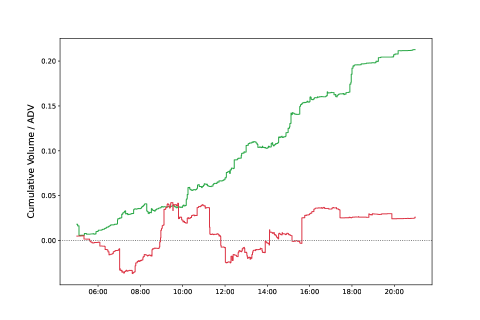
Figure 2: Two realizations of GBPUSD order flow, one which is a martingale (in red) and one with momentum (in green).

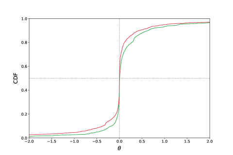
Figure 3: CDF of $\hat{\theta}$ for the same days as in Figure 2.

We also consider the hedging (externalization) flow by the desk during the same time period and find the correlation coefficient of -0.25 between $d^{2}Z_{t}/dt^{2}$ and $q_{t}$. Understandably, it is not easy to fully remove pricing sensitivity from the flow (and thus skew driven flow changes) but the observed negative correlation can serve as a reasonable estimate for $\hat{b}$ parameter in (2.3).

4.2 Numerical results

In this section, we investigate numerical simulations of the trading period under various parameter choices. In the first scenario we consider the case where the toxicity $\theta^{q}$ in (2.3) exhibits reversion, which makes filtering more challenging, due to the low drift to noise ratio. In the second scenario, the toxicity exhibits momentum. This means the toxicity follows a more predictable pattern and thus filtering leads to better estimates. The third scenario concerns a shorter trading period and it also includes a price predictive signal (alpha). Finally, the last scenario considers an agent who somehow has access to the true value of the inflow’s drift.

Scenario 1: mean-reverting toxicity.

The first scenario represents our benchmark. The agent has one trading day ($T=1$), and starts the day with no initial inventory. The initial values for $X,Z,\theta,Y,P,$ are as shown in Table 1.

$x$	$z$	$\theta_{0}$	$y$	$p$
0	0	0.1	0	1.27

Table 1: Initial conditions used for all scenarios

We model the local martingale component $\overline{M}$ in (2.1) of the unaffected price $P$ as a Brownian motion

$$\overline{M}_{t}=\sigma_{M}W^{M}_{t},$$ (4.1)

and choose $\sigma_{M}=6.3\cdot 10^{-3}$, which corresponds to 10% annualized. We set the signal to be $A=0$. The volatility of inflow in (2.2) is taken to be $\sigma=0.1$, following the analysis in 4.1. The coefficients in the dynamics of $\theta^{q}$ are then shown in Table 2. The price impact parameters in (2.6) and (2.7) are chosen to represent those of a liquid market and are also given in Table 2. They are consistent with value reported by [31] and internal desk estimations.

$a$	$b$	$c$	$d$	$\epsilon$	$\beta$	$\lambda$
-0.4	-0.2	0	0.01	0.01	10	0.1

Table 2: Coefficients in $\theta^{q}$ and price impact parameters

The parameter $a$ represents momentum in the drift of the inflow, so that for $a<0$ on average toxicity will decrease from its positive initial value as the day progresses. The parameter $b$ represents the market’s response to the outflow trades. As discussed in Section 2, this is chosen to be negative to model the behaviour of predatory traders. Finally, the penalisation parameter in (2.9) is set fairly high to $\alpha=100$ to strongly encourage the agent to unwind all of their inventory at the end of the trading period.

We simulate the model outputs, including the optimal trading rate by using Corollary 3.9. We notice that, due to the positive $\theta^{q}$ throughout the simulation, the cumulative inflow $Z^{q}$ builds. Over the day, the agent then progressively sells this inflow, leading cumulative $Q^{q}$ to decline. The result is that the agent manages to maintain inventory $X^{q}$ very close to zero across the entire day. All of these processes are shown on the lower panel of Figure 4.

The agent also continuously considers transient price impact $Y^{q}$, which is allowed to build early in the simulation and then carefully managed. At the end of the day, the agent decides that avoiding terminal penalty is more cost effective than managing transient price impact, and thus $Y^{q}$ builds rapidly in magnitude. This is shown in the upper panel, via the difference between the price with transient price impact, and the unaffected price $P$.

This scenario is a marginally more challenging environment for filtering than Scenario 2, where toxicity exhibits momentum. Without a clear trend for the toxicity $\theta^{q}$, the true value is harder to estimate. Nonetheless, the filter $\hat{\theta}^{q}$ still performs well, as can be seen on the middle panel of Figure 4. Due to calibration of the weights on the innovation process done in Appendix A (and presented in Theorem 3.1), the estimate is kept close in magnitude to the true value. The terminal inventory $X^{q}_{T}$ is therefore still very close to zero as seen on the third panel of Figure 4.

In what follows, we refer to trading P&L of a single realisation of the model, which is defined as the negative of the trading cost (without the risk aversion term)

$$P\&L_{\text{trading}}^{q}=P_{T}X^{q}_{T}-\int_{0}^{T}S_{t}dQ^{q}_{t}.$$ (4.2)

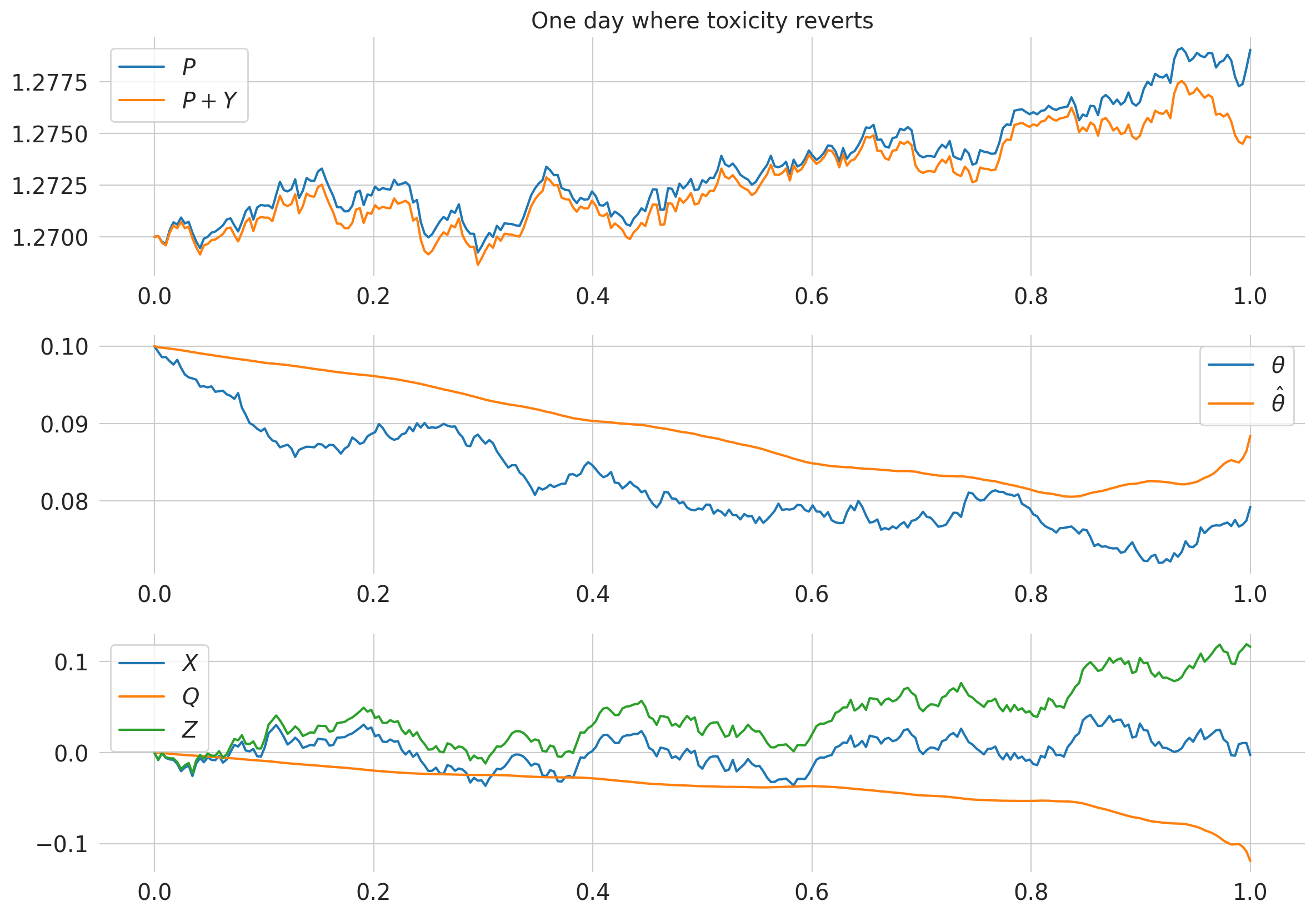
Figure 4: A simulation of the model’s state variables at optimality in the case of mean-reverting toxicity. The trading P&L in this simulation is 0.1311.

Scenario 2: momentum toxicity.

In the second scenario, all parameters from the previous scenario are unchanged except the value of $a$ which is now set to $0.4$. The toxicity $\theta^{q}$ now has substantial momentum, and doubles in magnitude over the day. This pattern is much easier to filter for, due to the higher drift to noise ratio of $\theta^{q}$ as seen on the middle panel of Figure 5. The cumulative inflow $Z^{q}$ now also reaches double the value in the previous scenario, which gives the agent more inventory to sell. At first this may seem a good outcome, but the transient price impact accumulated by the agent is larger than in the previous case, as seen on the upper panel of Figure 5. Furthermore, the temporary price impact costs are much larger. These costs associated with price impact lead to a higher cost functional than in the case where toxicity reverts.

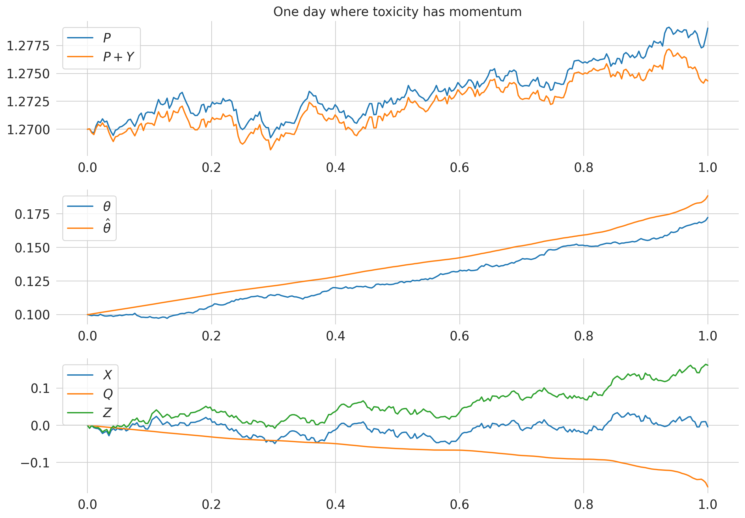
Figure 5: A simulation of the model where toxicity exhibits momentum. The trading P&L in this simulation is 0.2167.

Scenario 3: incorporating alphas.

In contrast to the previous two scenarios considered, we now look at an agent who only trades for a fraction of the whole day ($T=0.02$) and the terminal inventory penalty is reduced to $\alpha=1$. The volatilities of the inflow $\sigma$ in (2.2), price process $\sigma_{M}$ in (4.1) and toxicity $d$ in (2.3) have all been scaled by a factor of $\sqrt{0.02}$. The most notable change is that we assume the agent has access to a finite-variation price predicting signal over this window. The signal $A$ is expressed as the integral of an Ornstein-Uhlenbeck process, as described in (3.27) and (3.28). The parameters appearing in (3.28) are $\kappa=0.02$ and $\ell=\sqrt{0.02}$. All other parameters are identical to those of Scenario 1. Since $\epsilon$ is of the same magnitude as in the previous scenarios, and $\alpha$ is lower than in the one-day scenarios described above, the agent has less incentive to unwind all of the inventory at the end of the trading period. However, in this simulation, the inventory still terminates close to zero, as seen on the last panel of Figure 6. Additionally, due to the relatively small volume traded, the transient price impact $Y^{q}$ is much smaller than in the case with toxicity reversion over an entire day.

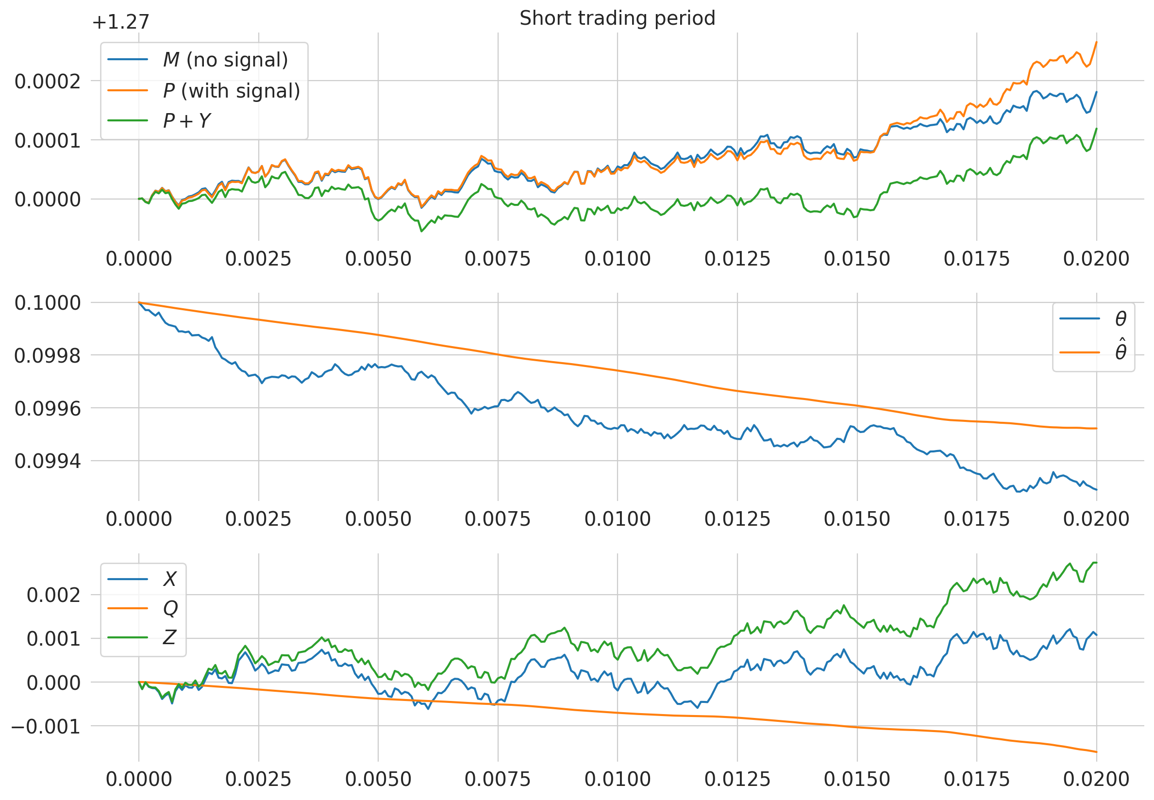
Figure 6: A simulation of the model over a short time horizon with a signal. The trading P&L of this simulation is 0.0034.

Comparison to the full information case.

We compare the partially observable model to the case where the agent has access to the true value of the toxicity $\theta^{q}$ and does not need to filter. Specifically, the problem is unchanged from the partially observable stochastic control problem described in Section 2, except for the class of admissible controls, which is now given by

$$\mathcal{A}:=\left\{q\,:\,q\textrm{ is }\{\mathcal{F}_{t}\}_{t\in[0,T]}-\textrm{ prog measurable s.t. }\mathbb{E}\Big{[}\int_{0}^{T}q_{t}^{2}dt\Big{]}<\infty\right\}.$$ (4.3)

In this case, there is no need to obtain filtering processes. The optimal control is of the same form. This is because the filtering is about finding the best weights to put on the innovation process, which is a martingale and thus does not affect the agent’s decisions. This naturally leads us to the corresponding result to Theorem 3.8.

Theorem 4.1.

Let assumptions analogous to 3.4 and 3.6 be satisfied. Then, the optimal control $q^{*}$ in the full information case is given by

$$q^{*}_{t}=g^{X}(t)X^{q*}_{t}+g^{\theta}(t)\theta^{q*}_{t}+g^{Y}(t)Y^{q*}_{t}+g^{P}(t)P_{t}+\mathbb{E}\left[\int_{t}^{T}g^{A}(s,t)dA_{s}\Big{|}\mathcal{F}_{t}\right].$$ (4.4)

where $g^{X},g^{\theta},g^{Y},g^{P}$ and $g^{A}$ are the same deterministic functions as in Theorem 3.8, and are given in Appendix C.

We first plot the optimal model outputs which follow from (4.4), using model parameters identical to those of Scenario 1. We see that, due to the strong performance of the filter in the partially observable case shown in Scenario 1, the performance and trading decisions made are almost identical.

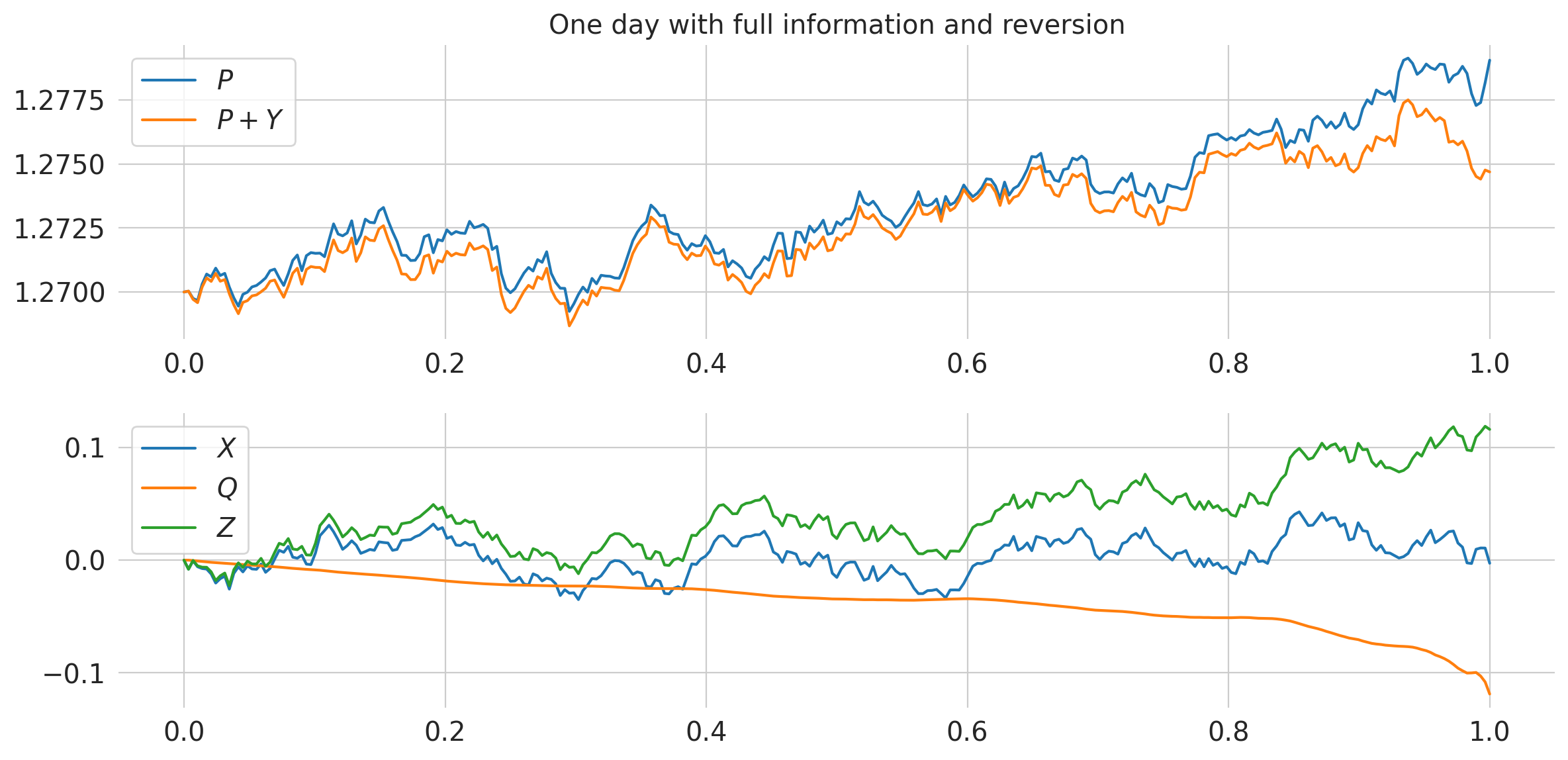
Figure 7: A simulation of the model where toxicity reverts and the agent has access to the true value of $\theta$. The trading P&L in this simulation is 0.1311, which is equal to four significant digits to the trading P&L for the simulation shown in Figure 4.

The performance of the optimal strategy under each of the Scenarios 1-3 is shown in Table 3. The Monte Carlo estimate of the cost functional, with 2,000 simulations used for each, is shown on the right hand side. One takeaway is that the case where toxicity $\theta^{q}$ exhibits momentum (and subsequently the cumulative inflow $Z^{q}$ is of larger magnitude) has a higher cost functional than the case where toxicity reverts to zero. The other main takeaway from Table 3 is that the performance of the agent who does not know the true value of $\theta$ is almost identical to that of the agent with full information. This is a consequence of the strong performance of filtering in our model.

Scenario	Partial information	Full information
Toxicity reverts	-0.1089	-0.1089
Toxicity has momentum	0.5441	0.5442
Short period with signal	-0.0026	-0.0026

Table 3: Monte Carlo estimates, to four significant figures, of the cost functional $\mathcal{C}$ in (2.9) using 2000 simulations for each scenario, where $\theta$ is unknown and known.

4.3 Externalization for Mitigating the Risk

Stochastic inflow carries the following P&L exposure for the book

$$P\&L^{0}=-\int_{0}^{T}P_{t}\,dZ^{0}_{t},$$ (4.5)

which is associated to risk of holding inventory. The agent can reduce this risk by trading, with the expense of price impact costs. Total P&L includes in addition to $P\&L_{\text{trading}}^{q}$ in (4.2) also the trading costs and the influence of the market impact on the flow:

$$P\&L_{\text{total}}^{q}=P\&L_{\text{trading}}^{q}-\int_{0}^{T}\left(P_{t}+Y^{q}_{t}\right)\,dZ^{0}_{t}.$$ (4.6)

In our study, we have minimised the trading costs with an additional risk aversion penalty. Figure 8 compares the distributions of P&L components for the parameter choices of Scenario 1 obtained by Monte Carlo simulation (2000 trajectories). The total P&L can be seen to have a significantly lower variance than P&L without trading demonstrating the suitability of externalisation for managing the overall risk for the book.

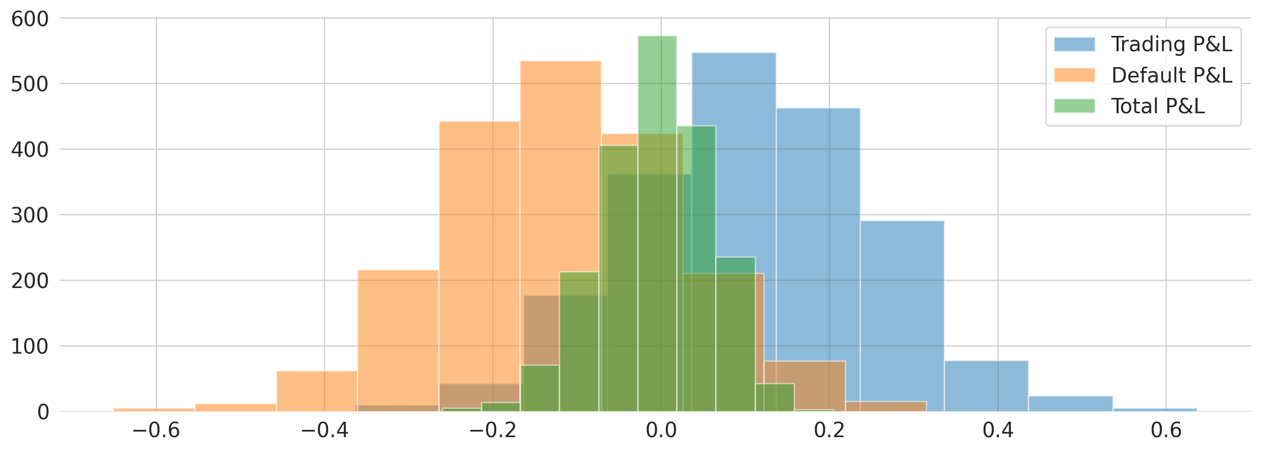
Figure 8: Probability distribution of total P&L, trading P&L and default P&L without trading for the parameters in Scenario 1.

4.4 A Naive Agent and Model Misspecification

Lastly, we consider an agent who believes $b=0$, while the true value is $b=-0.2$ in this case. The naive agent believes that there is no market response to outflow trades and thus no ability to influence inflow. This naive agent then filters and trades accordingly. All other parameters are the same as those of the case where toxicity $\theta^{q}$ reverts to zero, described in Scenario 1 of Section 4.2. This leads to worse estimates of $\theta^{q}$ than if they had used the correct value of $b$. The poor performance of the filter is clear in the second panel of Figure 9, especially when compared to the other scenarios in Section 4.2. The naive agent in this simulation achieves a trading P&L of 0.0912, which is lower than in Scenario 1, which uses the same parameters but considers a agent who knows the correct value of $b$. This can partially be explained by the worse performance of the filter, especially at the end of the trading period, where fast unwinding leads to a change in $\theta$ which the naive agent is unaware of.

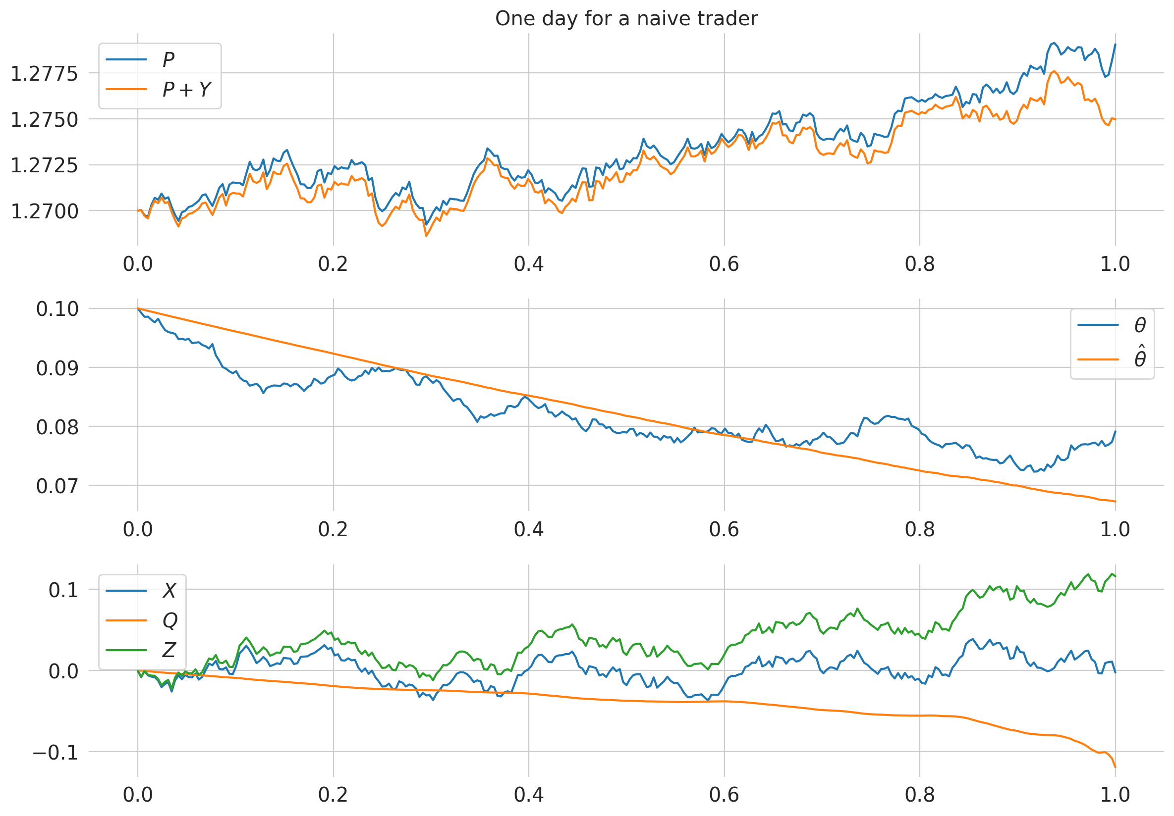
Figure 9: A simulation of the model for a naive agent who believes $b=0$ when in fact $b=-0.2$. The trading P&L for this simulation is 0.0912, which is $30\%$ lower than in Scenario 1

We also compare the performance of the naive agent with one who knows the true value of $b$, for example from calibration prior to the start of the day. Table 4 shows the Monte Carlo estimate of the cost functional found using 2000 simulations in both the case of the naive agent and the optimal agent. We show negative values of $b$ which represent the ‘predatory trading’ effect discussed in Section 2, but positive values of $b$ are also possible providing Assumptions 3.4, 3.6 and 3.7 are satisfied.

We see that both the naive and optimal agent’ performance is better when $b$ is of larger magnitude. The agent then has the ability to influence the inventory $X^{q}$ more strongly via $Z^{q}$, allowing for more flexibility when controlling transient price impact $Y^{q}$. One example is that the agent has been selling (as is usually the case when $\theta_{0}>0$) and thus transient price impact $Y^{q}$ has become negative. The agent can then buy, worsening the long inventory position, to offset the transient price impact. In the case where $b$ is far from zero, the increased inventory from buying will be partially offset by the market feedback, while the price impact will still be reduced in magnitude. Such a trading decision may lead to more trading costs later if $b$ is close to zero, due to the need to unwind the acquired inventory. Note that even a naive agent may decide to make such a trade due to the necessity of controlling transient price impact and the possibility of inventory internalisation due to inflow. We also observe, as expected, that the optimal agent consistently achieves a lower cost functional.

We also present in Figure 10 a histogram of the trading P&L for the case where $b=-0.2$, but a naive agent believes $b=0$. Due to the imperfect trading strategy used by the naive agent, variance is higher than for the agent who knows the correct value of $b$. The naive agent’s P&Ls also have a negative skew.

True $b$	Naive cost MC	Optimal cost MC
-0.1	-0.0677	-0.0988
-0.2	-0.0601	-0.1103
-0.3	-0.0663	-0.1132
-0.4	-0.0818	-0.1083

Table 4: The sensitivity of the model to the market’s trading response, and the impact of misspecification. In each case, the naive agent believes $b=0$ and filters and unwinds accordingly, while the optimal agent filters and unwinds using the correct value of $b$.

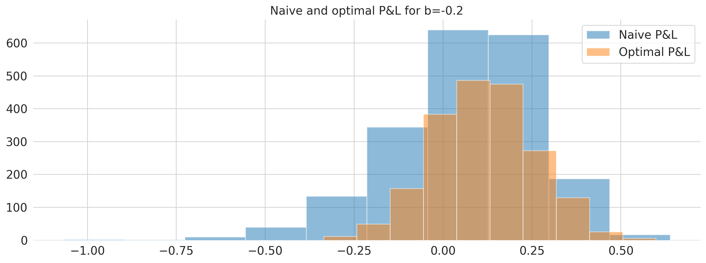
Figure 10: Histogram of Trading P&L for the naive agent (blue) and the optimal agent (orange) for true value of $b=-0.2$.

5 Conclusion

In this paper we have considered a model for a central trading desk which aggregates the inflow of clients’ orders with unobserved toxicity. The desk then faces a continuous dilemma of whether to internalise their inventory and save on transaction costs and market impact but bear the risk of adverse selection, or to externalise in a cost effective manner and reduce risk. Using institutional FX flow as an example, we showed that the probabilistic properties of the order flow’s drift can randomly change from mean-reverting to momentum-driven from day to day, while the distribution parameters of the toxicity remain stable throughout a one year horizon. Our empirical study also pointed out that unwinding the order flow creates a significant feedback effect on the flow.

The desk’s typical objective is to maximise the risk-adjusted daily P&L. As in the current CRB setting the desk does not influence the flow directly, we have considered a utility maximizing trading P&L subject to end of the day inventory penalization. We have formulated the aforementioned setting as a partially observable stochastic control problem and solved it in two steps. First, we derived the filtered dynamics of the inventory and toxicity, projected to the observed filtration, which turns the stochastic control problem into a fully observed problem. Then we used a variational approach in order to derive the unique optimal trading strategy. We have illustrated our results for various scenarios in which the desk is facing momentum and mean-reverting toxicity. We have shown that feedback of externalization has a prominent effect on the P&L, even for small values of the feedback parameter. We then studied the P&L performance gap between the partially observable problem and the full information case and found the regret to be of order $0.01\%$ for all tested market scenarios. Incorporating continuous assessment of flow toxicity into optimal control in real time offers a dynamic solution to internalization-externalization dilemma.

Appendix A Proof of Theorem 3.1

The proof of Theorem 3.1 uses ides the proof of Theorem 3.1 of [34]. The main idea in this approach is to use the innovation process $V$ in (3.9) as the noise term of the filtering processes $\hat{\mathbb{X}}^{q}$ in (3.4) which is weighted by a time-varying deterministic process, which is a solution to a matrix differential equation as in (3.11). These weights can be thought of as analogous to the Kalman gain originally studied in Kalman and Bucy [24]. The weights are found using the Fujisaki-Kallianpur-Kunita theorem [33] and ideas from stochastic analysis.

In the first step, we consider an affine transformation of the innovation process and prove that it is a standard Brownian motion. Recall that the class of admissible unwind strategies $\mathcal{A}$ was defined in (2.4). Recall that $V$ was defined in (3.9).

Lemma A.1.

For any $q\in\mathcal{A}$ the process

$$\widetilde{V}_{t}:=\sigma^{-1}(V_{t}-V_{0}),\quad t\geq 0,$$ (A.1)

is a $\{\mathcal{Y}^{q}_{t}\}_{t\in[0,T]}$-Brownian Motion.

Proof.

Let $q\in\mathcal{A}$. First note that from (3.9) it follows that $(V_{t})_{t\in[0,T]}$ is $(\mathcal{Y}^{q}_{t})_{t\in[0,T]}$ adapted. From (3.4), (3.6) and (3.9) it follows that,

$$V_{t}=\int_{0}^{t}\mathbf{e}_{1}^{\top}\widetilde{\mathbb{X}}^{q}_{s}ds+\sigma W^{Z}_{t}.$$ (A.2)

Since $\widetilde{\mathbb{X}}^{q}\perp\mathcal{Y}^{q}$ and $\hat{\mathbb{X}}^{q}$ is an unbiased estimator of $\mathbb{X}^{q}$ we get from (A.2) by using the tower rule

$$\mathbb{E}\left[V_{t}-V_{s}|\mathcal{Y}^{q}_{s}\right]=\mathbb{E}\left[\mathbb{E}\left[W^{Z}_{t}-W^{Z}_{s}|\mathcal{F}_{s}\right]|\mathcal{Y}^{q}_{s}\right]+\mathbb{E}\left[\int_{s}^{t}\mathbf{e}_{1}^{\top}\widetilde{\mathbb{X}}^{q}_{r}dr\right]=0,$$ (A.3)

where we have used (3.4) and Fubini’s theorem in the second equality. This shows that $\tilde{V}$ is a $\{\mathcal{Y}^{q}_{t}\}_{t\in[0,T]}$-martingale.

Next we use Itô’s lemma, (A.1) and (A.2) to get,

$$\begin{split}\widetilde{V}_{t}^{2}-\widetilde{V}_{s}^{2}&=2\int_{s}^{t}\sigma^{-1}\mathbf{e}_{1}^{\top}\widetilde{\mathbb{X}}^{q}_{r}\widetilde{V}_{r}dr+2\int_{s}^{t}\widetilde{V}_{r}dW^{Z}_{r}+(t-s),\quad\textrm{for all }0\leq s\leq t\leq T.\end{split}$$ (A.4)

Then with applications of Fubini’s Theorem and the tower rule we get for $0\leq s\leq t\leq T$,

$$\mathbb{E}\left[\widetilde{V}_{t}^{2}-\widetilde{V}_{s}^{2}\big{|}\mathcal{Y}^{q}_{s}\right]$$ (A.5)

$$=2\int_{s}^{t}\sigma^{-1}\mathbf{e}_{1}^{\top}\mathbb{E}\left[\widetilde{\mathbb{X}}^{q}_{r}\widetilde{V}_{r}\big{|}\mathcal{Y}^{q}_{s}\right]dr+2\mathbb{E}\left[\int_{s}^{t}\widetilde{V}dW^{Z}_{r}\Big{|}\mathcal{Y}^{q}_{s}\right]+(t-s)$$

$$=2\int_{s}^{t}\sigma^{-1}H\mathbb{E}\left[\mathbb{E}\left[\widetilde{\mathbb{X}}^{q}_{r}\right]\tilde{V}_{r}\big{|}\mathcal{Y}^{q}_{s}\right]dr+2\mathbb{E}\left[\mathbb{E}\left[\int_{s}^{t}\widetilde{V}dW^{Z}_{r}\Big{|}\mathcal{F}_{s}\right]\Big{|}\mathcal{Y}^{q}_{s}\right]+(t-s)$$

$$=(t-s),$$

where in the last inequality we have used the fact that $W^{Z}$ is an $(\mathcal{F}_{t})_{t\in[0,T]}$-Brownian motion and the fact that $\widetilde{\mathbb{X}}$ has zero mean by (3.4).

From (A.5) it follows that $\tilde{V}$ is a $\{\mathcal{Y}^{q}_{t}\}_{t\in[0,T]}$-Brownian Motion by Lévy’s Characterization theorem. ∎

Recall the dynamics of $\mathbb{X}^{q}$ from (3.2) and that $\hat{\mathbb{X}}^{q}$ was defined in (3.4). We introduce the $\{\mathcal{Y}^{q}_{t}\}_{t\in[0,T]}$-progressively measurable process,

$$\Lambda_{t}:=\hat{\mathbb{X}}^{q}_{t}-x-\int_{0}^{t}(A_{s}\hat{\mathbb{X}}^{q}_{s}+B_{s}q_{s})ds,\quad 0\leq t\leq T.$$ (A.6)

Lemma A.2.

The process $\Lambda$ is a $\{\mathcal{Y}^{q}_{t}\}_{t\in[0,T]}$-martingale.

Proof.

From (3.2), (3.4) and (A.6), Fubini’s theorem it follows that for any $0\leq s\leq t\leq T$ we have,

$$\mathbb{E}\left[\Lambda_{t}-\Lambda_{s}|\mathcal{Y}^{q}_{s}\right] =\mathbb{E}\left[\hat{\mathbb{X}^{q}_{t}}-\hat{\mathbb{X}}^{q}_{s}|\mathcal{Y}^{q}_{s}\right]-\mathbb{E}\left[\int_{s}^{t}(A_{r}\hat{\mathbb{X}}^{q}_{r}+B_{r}q_{r})dr\Big{|}\mathcal{Y}^{q}_{s}\right]$$ (A.7)

$$=\mathbb{E}\left[\mathbb{X}^{q}_{t}-\mathbb{X}^{q}_{s}|\mathcal{Y}^{q}_{s}\right]-\int_{s}^{t}\mathbb{E}\left[A_{r}\hat{\mathbb{X}}^{q}_{r}+B_{r}q_{r}|\mathcal{Y}^{q}_{s}\right]dr$$

$$=\mathbb{E}\left[\mathbb{X}^{q}_{t}-\mathbb{X}^{q}_{s}|\mathcal{Y}^{q}_{s}\right]-\int_{s}^{t}\mathbb{E}\left[A_{r}\mathbb{X}^{q}_{r}+B_{r}q_{r}|\mathcal{Y}^{q}_{s}\right]dr$$

$$=\mathbb{E}\bigg{[}\int_{s}^{t}(A_{r}\mathbb{X}^{q}_{r}+B_{r}q_{r})dr$$

$$\qquad+C_{r}(W^{Z}_{t}-W^{Z}_{s})+D_{r}(W^{\theta}_{t}-W^{\theta}_{s})\Big{|}\mathcal{Y}^{q}_{s}\bigg{]}$$

$$\qquad-\int_{s}^{t}\mathbb{E}\left[A_{r}\mathbb{X}^{q}_{r}+B_{r}q_{r}|\mathcal{Y}^{q}_{s}\right]dr$$

$$=0,$$

Where we have used the tower rule in the last equality. This concludes the result. ∎

We recall that $\mathbf{e}_{1}$ and $\Sigma_{t}$ were defined in (3.7) and (3.8), respectively.

Proposition A.3.

There exists a $\{\mathcal{Y}^{q}_{t}\}_{t\in[0,T]}$-progressively measurable process $\gamma=(\gamma_{t})_{t\in[0,T]}$ such that

$$\Lambda_{t}=\int_{0}^{t}\gamma_{s}\sigma^{-2}dV_{s},\quad\textrm{for all }\ 0\leq t\leq T.$$ (A.8)

Moreover, $\gamma$ is given by,

$$\gamma_{t}=\Sigma_{t}\mathbf{e}_{1}+\sigma C_{t},\quad 0\leq t\leq T.$$ (A.9)

Proof.

From the Fujisaki-Kallianpur-Kunita theorem (see e.g. Theorem 8.4 from Chapter V1.8 of [33]) it follows that there exists a process $\gamma$ which is $\{\mathcal{Y}^{q}_{t}\}_{t\in[0,T]}$-progressively measurable such that (A.8) holds. Let $(\zeta_{t})_{t\in[0,T]}$ be square-integrable, $\{\mathcal{Y}^{q}_{t}\}_{t\in[0,T]}$-progressively measurable and fixed, but arbitrary. Define

$$\eta_{t}=\int_{0}^{t}\zeta_{s}\sigma^{-2}dV_{s},\quad 0\leq t\leq T.$$ (A.10)

From Lemma A.1 it follows that $\eta$ is a $\{\mathcal{Y}^{q}_{t}\}_{t\in[0,T]}$-martingale. From (A.8) and (A.10) we have

$$\mathbb{E}\left[\Lambda_{t}\eta_{t}\right]=\mathbb{E}\left[\int_{0}^{t}\gamma_{s}\sigma^{-2}\zeta_{s}ds\right]$$ (A.11)

Plugigng in (A.6) we get,

$$\mathbb{E}\left[\Lambda_{t}\eta_{t}\right]=\mathbb{E}\left[\hat{\mathbb{X}}^{q}_{t}\eta_{t}\right]-\mathbb{E}\left[\int_{0}^{t}\left(A_{s}\hat{\mathbb{X}}^{q}_{s}+B_{s}q_{s}\right)\eta_{t}ds\right].$$ (A.12)

Using the martingale property of $\eta$ and (3.4), we have for $0\leq s\leq t\leq T$,

$$\mathbb{E}\left[\hat{\mathbb{X}}^{q}_{s}\eta_{t}\right]=\mathbb{E}\left[\mathbb{E}\left[\hat{\mathbb{X}}^{q}_{s}\eta_{t}|\mathcal{Y}^{q}_{s}\right]\right]=\mathbb{E}\left[\mathbb{E}\left[\mathbb{X}^{q}_{s}|\mathcal{Y}^{q}_{s}\right]\mathbb{E}\left[\eta_{t}|\mathcal{Y}^{q}_{s}\right]\right]=\mathbb{E}\left[\mathbb{X}^{q}_{s}\eta_{s}\right],$$ (A.13)

and

$$\mathbb{E}\left[B_{s}q_{s}\eta_{t}\right]=\mathbb{E}\left[(B_{s}q_{s})\eta_{s}\right].$$ (A.14)

Plugging in (A.13) and (A.14) into (A.12) we get,

$$\mathbb{E}\left[\Lambda_{t}\eta_{t}\right]=\mathbb{E}\left[\hat{\mathbb{X}}^{q}_{t}\eta_{t}\right]-\mathbb{E}\left[\int_{0}^{t}\left(A_{s}\hat{\mathbb{X}}^{q}_{s}+B_{s}q_{s}\right)\eta_{s}ds\right]$$ (A.15)

From (A.10) and (A.2) we get

$$d\eta_{t}=\zeta_{t}\sigma^{-2}\left(\mathbf{e}_{1}^{\top}\widetilde{\mathbb{X}}^{q}_{t}dt+\sigma dW^{Z}_{t}\right).$$ (A.16)

From (3.2), (A.16) and by using integration by parts it follows that,

$$\begin{split}&\mathbb{E}\left[\mathbb{X}^{q}_{t}\eta_{t}\right]\\ &=\mathbb{E}\left[\int_{0}^{t}\left(A_{s}\mathbb{X}_{s}+B_{s}q_{s}\right)\eta_{s}ds+\int_{0}^{t}\mathbb{X}^{q}_{s}(\widetilde{\mathbb{X}}_{s}^{q})^{\top}\mathbf{e}_{1}\sigma^{-2}\zeta_{s}ds+\int_{0}^{t}C_{s}\sigma^{-1}\zeta_{s}ds\right].\end{split}$$ (A.17)

Using (3.4), (3.8), $\widetilde{\mathbb{X}}\perp\mathcal{Y}^{q}$, the fact that $\widetilde{\mathbb{X}}$ has zero mean we get

$$\mathbb{E}\left[\int_{0}^{t}\mathbb{X}_{s}(\widetilde{\mathbb{X}}^{q}_{s})^{\top}\mathbf{e}_{1}\sigma^{-2}\zeta_{s}ds\right] =\mathbb{E}\left[\int_{0}^{t}(\widetilde{\mathbb{X}}^{q}_{s})(\widetilde{\mathbb{X}}^{q}_{s})^{\top}\mathbf{e}_{1}\sigma^{-2}\zeta_{s}ds+\int_{0}^{t}(\hat{\mathbb{X}}^{q}_{s})(\widetilde{\mathbb{X}}^{q}_{s})^{T}\mathbf{e}_{1}\sigma^{-2}\zeta_{s}ds\right]$$ (A.18)

$$=\mathbb{E}\left[\int_{0}^{t}\Sigma_{s}\mathbf{e}_{1}\sigma^{-2}\zeta_{s}ds\right].$$

Plugging in (A.18) into (A.16) and using again the fact that $\widetilde{\mathbb{X}}\perp\mathcal{Y}^{q}$ that $\widetilde{\mathbb{X}}$ has zero mean we get,

$$\mathbb{E}\left[\hat{\mathbb{X}}^{q}_{t}\eta_{t}\right]=\mathbb{E}\left[\int_{0}^{t}\left(A_{s}X_{s}+B_{s}q_{s}\right)\eta_{s}ds+\int_{0}^{t}\Sigma_{s}\mathbf{e}_{1}\sigma^{-2}\zeta_{s}ds+\int_{0}^{t}C_{s}\sigma^{-1}\zeta_{s}\right].$$ (A.19)

Using this as well as (A.11) and (A.12) leaves that

$$\gamma_{t}=\Sigma_{t}\mathbf{e}_{1}+\sigma C_{t},$$ (A.20)

since $\zeta$ was chosen arbitrarily. This completes the proof. ∎

Proof of Theorem 3.1.

Using (A.6), (A.8) with (A.9) the SDE for $\hat{\mathbb{X}}^{q}$ we get

$$d\hat{\mathbb{X}}^{q}_{t}=\left(\Sigma_{t}\mathbf{e}_{1}+\sigma C_{t}\right)\sigma^{-2}\mathbf{e}_{1}^{\top}\widetilde{\mathbb{X}}^{q}dt+\left(\Sigma_{t}\mathbf{e}_{1}+\sigma C_{t}\right)\sigma^{-1}dW^{Z}_{t}+\left(A_{t}\hat{\mathbb{X}}^{q}_{t}+B_{t}q_{t}\right)dt.$$ (A.21)

Using (A.21) and (A.2) we recover (3.10). By subtracting (A.21) from (3.2), recalling (3.4) we get,

$$d\widetilde{\mathbb{X}}_{t}=\left(A_{t}-\left(\Sigma_{t}\mathbf{e}_{1}+\sigma C_{t}\right)\sigma^{-2}\mathbf{e}_{1}^{\top}\right)\widetilde{\mathbb{X}}^{q}_{t}dt-\Sigma_{t}\mathbf{e}_{1}\sigma^{-1}dW^{Z}_{t}+D_{t}dW^{\theta}_{t}.$$ (A.22)

Next we can use (A.22), integration by parts and Fubini’s theorem in order to derive the dynamics of $\Sigma$ in (3.8), recalling that $\widetilde{\mathbb{X}}^{q}_{0}=0$,

$$\Sigma_{t} =\mathbb{E}\bigg{[}\int_{0}^{t}\left(A_{s}-\left(\Sigma_{s}\mathbf{e}_{1}+\sigma C_{s}\right)\sigma^{-2}\mathbf{e}_{1}^{\top}\right)\widetilde{\mathbb{X}}^{q}_{s}\left(\widetilde{\mathbb{X}}^{q}_{s}\right)^{\top}ds$$ (A.23)

$$\qquad+\int_{0}^{t}\widetilde{\mathbb{X}}_{s}\left(\widetilde{\mathbb{X}}^{q}_{s}\right)^{\top}\left(A_{s}-\left(\Sigma_{s}\mathbf{e}_{1}+\sigma C_{s}\right)\sigma^{-2}\mathbf{e}_{1}^{\top}\right)^{\top}ds$$

$$\qquad+\int_{0}^{t}\sigma^{-2}\Sigma_{s}\mathbf{e}_{1}\mathbf{e}_{1}^{\top}\Sigma_{s}ds+\int_{0}^{t}D_{s}D_{s}^{\top}ds\bigg{]}$$

$$=\int_{0}^{t}\left(A_{s}-\left(\Sigma_{s}\mathbf{e}_{1}+\sigma C_{s}\right)\sigma^{-2}\mathbf{e}_{1}^{\top}\right)\Sigma_{s}ds+\int_{0}^{t}\Sigma_{s}\left(A_{s}-\left(\Sigma_{s}\mathbf{e}_{1}+\sigma C_{s}\right)\sigma^{-2}\mathbf{e}_{1}^{\top}\right)^{\top}ds$$

$$\quad+\int_{0}^{t}\sigma^{-2}\Sigma_{s}\mathbf{e}_{1}\mathbf{e}_{1}^{\top}\Sigma_{s}ds+\int_{0}^{t}D_{s}D_{s}^{\top}ds$$

$$=\int_{0}^{t}\left(A_{s}-\sigma^{-1}C_{s}\mathbf{e}_{1}^{\top}\right)\Sigma_{s}ds+\int_{0}^{t}\Sigma_{s}\left(A_{s}-\sigma^{-1}C_{s}\mathbf{e}_{1}^{\top}\right)^{\top}ds$$

$$\quad-\int_{0}^{t}\sigma^{-2}\Sigma_{s}\mathbf{e}_{1}\mathbf{e}_{1}^{\top}\Sigma_{s}ds+\int_{0}^{t}D_{s}D_{s}^{\top}ds.$$

Note that the above equation coincides with the Riccati equation (3.11). After applying a time change, Proposition 4.2 in [27] shows that this Riccati equation has a unique, positive semi-definite solution.

In order to complete the proof it is left to argue that (3.11) admits a unique solution. This follows from Lemma 2.1 of [34]. ∎

Proof of Corollary 3.2.

The equation for $\hat{X}^{q}$ in (3.12) follow directly from (3.1), (3.5) and (3.10). The following equation for $\hat{\theta}$ is derived by the same reasoning:

$$\hat{\theta}_{t}=\theta_{0}+\int_{0}^{t}\left(\kappa^{(1)}_{s}+\sigma^{-1}c_{s}\right)dV_{s}+\int_{0}^{t}\left(a_{s}\hat{\theta}_{s}+b_{s}q_{s}\right)ds.$$ (A.24)

Note that (3.13) solves (A.24). ∎

Appendix B Proof of Theorem 3.8

We prove Theorem 3.8 by using a variational approach in the spirit of [5, 29]. We first prove the essential convexity property for the cost functional (2.11).

Lemma B.1.

The cost functional $q\mapsto\mathcal{C}(q;p,s,y,z)$ in (2.11) is strictly convex on $\mathcal{A}$.

Proof.

The proof uses ideas from the proof of Lemma 10.1 in [30]. Integration by parts applied to the term $\hat{X}^{q}_{T}\left(\alpha\hat{X}^{q}_{T}-P_{T}\right)$ togather with (3.2) yields

$$\begin{split}-P_{T}\hat{X}^{q}_{T}+-\alpha\left(\hat{X}^{q}_{T}\right)^{2}&=-px+\alpha x^{2}-\int_{0}^{T}\hat{X}^{q}_{t}dP_{t}-\int_{0}^{T}P_{t}dV^{(2)}_{t}\\ &\quad-\int_{0}^{T}P_{t}\left(\hat{\theta}^{q}_{t}+q_{t}\right)dt+2\alpha\int_{0}^{T}\hat{X}^{q}_{t}dV^{(2)}_{t}\\ &\quad+2\alpha\int_{0}^{T}\hat{X}^{q}_{t}\left(\hat{\theta}^{q}_{t}+q_{t}\right)dt+-\alpha[\hat{X}^{q}]_{T}\end{split}$$ (B.1)

since $W^{Z}$ and $\overline{M}$ are independent. Substituting (B.1) into $\eqref{eq:cost Xhat}$ then gives us

$$\mathcal{C}(q;p,s,y,z) =-xp+\alpha x^{2}$$ (B.2)

$$\quad+\mathbb{E}_{p,s,y,z}\bigg{[}\int_{0}^{T}\left(-P_{t}\hat{\theta}^{q}_{t}+2\alpha\hat{X}^{q}_{t}\left(\hat{\theta}^{q}_{t}+q_{t}\right)+Y^{q}_{t}q_{t}+\frac{1}{2}\epsilon q_{t}^{2}\right)dt$$

$$\qquad\qquad+\int_{0}^{T}\left(2\alpha\hat{X}^{q}_{t}-P_{t}\right)dV^{(2)}_{t}-\int_{0}^{T}\hat{X}^{q}_{t}dP_{t}+\alpha[\hat{X}^{q}]_{t}\bigg{]}.$$

For convenience we omit the constants and the initial values notation in (B.2) and define,

$$\begin{split}\widetilde{\mathcal{C}}(q)&=\mathbb{E}\bigg{[}\int_{0}^{T}\left(-P_{t}\hat{\theta}^{q}_{t}+2\alpha\hat{X}^{q}_{t}\left(\hat{\theta}^{q}_{t}+q_{t}\right)+Y^{q}_{t}q_{t}+\frac{1}{2}\epsilon q_{t}^{2}\right)dt\\ &\qquad\quad+\int_{0}^{T}\left(2\alpha\hat{X}^{q}_{t}-P_{t}\right)dV^{(2)}_{t}-\int_{0}^{T}\hat{X}^{q}_{t}dP_{t}+\alpha[\hat{X}^{q}]_{t}\bigg{]}.\end{split}$$ (B.3)

Let $q,u\in\mathcal{A}$ such that $q\neq u$ $d\mathbb{P}\otimes ds$-a.e. on $\Omega\times[0,T]$. We will show that,

$$\widetilde{\mathcal{C}}\left(\delta q+(1-\delta)u\right)-\delta\widetilde{\mathcal{C}}(q)-(1-\delta)\widetilde{\mathcal{C}}(u)<0,\quad\textrm{for all }\delta\in(0,1),$$ (B.4)

which will prove the convexity of (2.11).

From (3.2) and (3.13) if follows that $\hat{\theta}^{\delta q+(1+\delta)u}_{t}=\delta\hat{\theta}^{q}_{t}+(1-\delta)\hat{\theta}^{u}_{t}$ and $\hat{X}^{\delta q+(1-\delta)u}=\delta\hat{X}^{q}+(1-\delta)\hat{X}^{u}$. We therefore get from (B.3),

$$\begin{split}&\widetilde{\mathcal{C}}\left(\delta q+(1-\delta)u\right)-\delta\widetilde{\mathcal{C}}(q)-(1-\delta)\widetilde{\mathcal{C}}(u)\\ &=-\delta(1-\delta)\mathbb{E}\bigg{[}\int_{0}^{T}\bigg{(}2\alpha\left(X^{q}_{t}-X^{u}_{t}\right)\left((\theta^{q}_{t}+q_{t})-(\theta^{u}_{t}+u_{t})\right)\\ &\qquad\qquad\qquad\quad+\left(Y^{q}_{t}-Y^{u}_{t}\right)\left(q_{t}-u_{t}\right)+\frac{1}{2}\epsilon\left(q_{t}-u_{t}\right)^{2}\bigg{)}dt\bigg{]}.\end{split}$$ (B.5)

Clearly the third term in the integral on the right-hand side of (B.5) is always strictly positive. Using (3.2) and integration by parts on the term $\big{(}\hat{X}^{q}_{T}-\hat{X}^{u}_{T}\big{)}^{2}$ yields

$$\int_{0}^{T}2\alpha\left(\hat{X}^{q}-\hat{X}^{u}_{t}\right)\left(\left(\hat{\theta}^{q}_{t}+q_{t}\right)-\left(\hat{\theta}^{u}_{t}+u_{t}\right)\right)dt=\alpha\left(\hat{X}^{q}_{t}-\hat{X}^{u}_{t}\right)^{2}>0.$$ (B.6)

Similarly, using (2.7) and integration by parts applied to the term $\left(Y^{q}_{T}-Y^{u}_{T}\right)^{2}$ further yields

$$\int_{0}^{T}\left(Y^{q}_{t}-Y^{u}_{t}\right)\left(q_{t}-u_{t}\right)dt=\frac{1}{2\lambda}\left(Y^{q}_{t}-Y^{u}_{t}\right)^{2}+\frac{\beta}{\lambda}\int_{0}^{T}\left(Y^{q}_{t}-Y^{u}_{t}\right)^{2}dt>0.$$ (B.7)

From (B.6), (B.7) and (B.5) we get (B.4). This concludes the result. ∎

For the sake of readability, we omit the use of the initial values notation in the cost functional (2.11) for the remainder of this section and refer to it as $\mathcal{C}(q)$. By Lemma B.1 and Proposition 1.2 from Chapter 2 of [19], $\mathcal{C}(\cdot)$ admits a unique minimiser $q^{*}\in\mathcal{A}$ if the Gateaux derivative satisfies (see e.g. Proposition 2.1 in Chapter II.1 of [19])

$$\langle\mathcal{C}^{\prime}(q^{*}),\eta\rangle:=\underset{\delta\rightarrow 0}{\lim}\left(\frac{\mathcal{C}(q^{*}+\delta\eta)-\mathcal{C}(q^{*})}{\delta}\right)=0,\quad\textrm{for all }\eta\in\mathcal{A}.$$ (B.8)

In the following lemma we derive an explicit expression for the Gateaux derivative.

Lemma B.2.

Let $\mathcal{C}$ be the cost functional in (2.11). Then, for any $\eta\in\mathcal{A}$ we have

$$\begin{split}\langle\mathcal{C}^{\prime}(q),\eta\rangle&=\mathbb{E}\bigg{[}\int_{0}^{T}\eta_{s}\bigg{(}P_{s}+\epsilon q_{s}+Y^{q}_{s}+\int_{s}^{T}e^{-\beta(t-s)}\lambda q_{t}dt\\ &\qquad-b_{s}P_{T}\int_{s}^{T}\exp\left(\int_{s}^{t}a_{r}dr\right)dt-P_{T}\\ &\qquad+2\alpha\left(b_{s}\hat{X}^{q}_{T}\int_{s}^{T}\exp\left(\int_{s}^{t}a_{r}dr\right)dt+\hat{X}^{q}_{T}\right)\bigg{)}ds\bigg{]}.\end{split}$$ (B.9)

Proof.

Let $\eta\in\mathcal{A}$. From (3.13), we have

$$\begin{split}\hat{\theta}_{t}^{q+\delta\eta}&=\theta_{0}\exp\left(\int_{0}^{t}a_{r}dr\right)+\int_{0}^{t}\exp\left(\int_{s}^{t}a_{r}dr\right)\left(\kappa^{(1)}_{s}+\sigma^{-1}c_{s}\right)dV_{s}\\ &\quad+\int_{0}^{t}b_{s}\exp\left(\int_{s}^{t}a_{r}dr\right)\left(q_{s}+\delta\eta_{s}\right)ds\\ &=\hat{\theta}^{q}_{t}+\delta\int_{0}^{t}b_{s}\exp\left(\int_{s}^{t}a_{r}dr\right)\eta_{s}ds.\end{split}$$ (B.10)

From (B.10) and (3.12), we get that

$$\begin{split}\hat{X}^{q+\delta\eta}_{t}&=x+\int_{0}^{t}\left(\kappa^{(2)}_{s}+1\right)dV_{s}+\int_{0}^{t}\left(\hat{\theta}^{q+\delta\eta}+q_{s}+\delta\eta_{s}\right)ds\\ &=x+\int_{0}^{t}\left(\kappa^{(2)}_{s}+1\right)dV_{s}\\ &\quad+\int_{0}^{t}\left(\hat{\theta}_{s}^{q}+\delta\int_{0}^{s}b_{s}\exp\left(\int_{r}^{s}a_{u}du\right)\eta_{r}dr+q_{s}+\delta\eta_{s}\right)ds\\ &=\hat{X}^{q}_{t}+\delta\int_{0}^{t}\left(\int_{0}^{s}b_{s}\exp\left(\int_{r}^{s}a_{u}du\right)\eta_{r}dr+\eta_{s}\right)ds.\end{split}$$ (B.11)

From (2.7) it follows that

$$Y^{q+\delta\eta}_{t}=Y^{q}_{t}+\delta\int_{0}^{t}e^{-\beta(t-s)}\lambda\eta_{s}ds.$$ (B.12)

Applying (B.10), (B.11) and (B.12) to (2.11), gives

$$\begin{split}&\mathcal{C}(q+\delta\eta)\\ &=\mathbb{E}\bigg{[}\int_{0}^{T}\left(P_{t}(q_{t}+\delta\eta_{t})+Y^{q+\delta\eta}_{t}(q_{t}+\delta\eta_{t})+\frac{1}{2}\epsilon(q_{t}+\delta\eta_{t})^{2}\right)dt\\ &\qquad-P_{T}\hat{X}^{q+\delta\eta}_{T}+\alpha\left(\hat{X}^{q+\delta\eta}_{T}\right)^{2}\bigg{]}\\ &=\mathbb{E}\bigg{[}\int_{0}^{T}\left(P_{t}(q_{t}+\delta\eta_{t})+\left(Y^{q}_{t}+\delta\int_{0}^{t}e^{-\beta(t-s)}\lambda\eta_{s}ds\right)(q_{t}+\delta\eta_{t})+\frac{1}{2}\epsilon(q_{t}+\delta\eta_{t})^{2}\right)dt\\ &\qquad-P_{T}\left(\hat{X}^{q}_{T}+\delta\int_{0}^{T}\left(\int_{0}^{t}b_{s}\exp\left(\int_{s}^{t}a_{r}dr\right)\eta_{s}ds+\eta_{t}\right)dt\right)\\ &\qquad+\alpha\left(\hat{X}^{q}_{T}+\delta\int_{0}^{T}\left(\int_{0}^{t}b_{s}\exp\left(\int_{s}^{t}a_{r}dr\right)\eta_{s}ds+\eta_{t}\right)dt\right)^{2}\bigg{]}.\end{split}$$ (B.13)

We therefore obtain,

$$\begin{split}&\frac{\mathcal{C}(q+\delta\eta)-\mathcal{C}(q)}{\delta}\\ &=\mathbb{E}\bigg{[}\int_{0}^{T}\bigg{(}P_{t}\eta_{t}+\frac{1}{2}\epsilon\left(2q_{t}\eta_{t}\right)+Y^{q}_{t}\eta_{t}+q_{t}\int_{0}^{t}e^{-\beta(t-s)}\lambda\eta_{s}ds\bigg{)}dt\\ &\qquad-P_{T}\left(\int_{0}^{T}\left(\int_{0}^{t}b_{s}\exp\left(\int_{s}^{t}a_{r}dr\right)\eta_{s}ds+\eta_{t}\right)dt\right)\\ &\qquad+\delta\bigg{(}\int_{0}^{T}\frac{1}{2}\epsilon\eta_{t}^{2}+\eta_{t}\int_{0}^{t}e^{-\beta(t-s)}\lambda\eta_{s}dsdt\bigg{)}\\ &\qquad+\alpha\bigg{(}2\hat{X}^{q}_{T}\int_{0}^{T}\int_{0}^{t}b_{s}\exp\left(\int_{s}^{t}a_{r}dr\right)\eta_{s}dsdt+2\hat{X}^{q}_{T}\int_{0}^{T}\eta_{t}dt\\ &\quad\qquad+\delta\bigg{(}\left(\int_{0}^{T}\int_{0}^{t}b_{s}\exp\left(\int_{s}^{t}a_{r}dr\right)\eta_{r}dsdt\right)^{2}+\left(\int_{0}^{T}\eta_{t}dt\right)^{2}\\ &\quad\qquad+2\left(\int_{0}^{T}\int_{0}^{t}b_{s}\exp\left(\int_{s}^{t}a_{r}dr\right)\eta_{s}dsdt\right)\left(\int_{0}^{T}\eta_{s}dt\right)\bigg{)}\bigg{)}\bigg{]}\end{split}$$ (B.14)

By taking $\delta\rightarrow 0$ we derive the Gateaux derivative,

$$\begin{split}\langle\mathcal{C}^{\prime}(q),\eta\rangle&=\mathbb{E}\bigg{[}\int_{0}^{T}\bigg{(}P_{t}\eta_{t}+\epsilon q_{t}\eta_{t}+Y^{q}_{t}\eta_{t}+q_{t}\int_{0}^{t}e^{-\beta(t-s)}\lambda\eta_{s}ds\bigg{)}dt\\ &\qquad-P_{T}\left(\int_{0}^{T}\left(\int_{0}^{t}b_{s}\exp\left(\int_{s}^{t}a_{r}dr\right)\eta_{s}ds+\eta_{t}\right)dt\right)\\ &\qquad+2\alpha\bigg{(}\hat{X}^{q}_{T}\int_{0}^{T}\int_{0}^{t}b_{s}\exp\left(\int_{s}^{t}a_{r}dr\right)\eta_{s}dsdt+\hat{X}^{q}_{T}\int_{0}^{T}\eta_{t}dt\bigg{)}\bigg{]}.\end{split}$$ (B.15)

We get (B.9) by applications of Fubini’s theorem. ∎

Before we state Lemma B.3, which charaterises the optimal trading rate as a solution to a system of FBSDEs, we introduce the following auxiliary processes:

$$\widetilde{M}_{t}:=\mathbb{E}\left[\left(\int_{0}^{T}\exp\left(\int_{0}^{s}a_{r}dr\right)ds\right)\left(2\alpha\hat{X}^{q*}_{T}-P_{T}\right)\Big{|}\mathcal{Y}^{q*}_{t}\right],\quad 0\leq t\leq T,$$ (B.16)

$$\begin{split}\widetilde{N}_{t}:=\mathbb{E}\left[\int_{0}^{T}e^{-\beta s}\lambda q^{*}_{s}dt\Big{|}\mathcal{Y}^{q*}_{t}\right],,\quad 0\leq t\leq T,\end{split}$$ (B.17)

and

$$\widetilde{R}_{t}:=\mathbb{E}\left[2\alpha\hat{X}^{q*}_{T}-P_{T}|\mathcal{Y}^{q*}_{t}\right],\quad 0\leq t\leq T.$$ (B.18)

Note that from (2.4), (3.12), (3.13) and since the functions $a,b,c,d,e$ are bounded by assumption, it follows that for any $q\in\mathcal{A}$, the processes $\widetilde{M},\widetilde{N}$ and $\widetilde{R}$ are square-integrable $\mathcal{Y}^{q*}$-martingales.

We further define

$$R_{t}=\widetilde{R}_{t}+N_{t}+M_{t},\quad 0\leq t\leq T.$$ (B.19)

where

$$\begin{split}M_{t}&=\int_{0}^{t}b^{\prime}_{s}\exp\left(-\int_{0}^{s}a_{r}dr\right)d\widetilde{M}_{s}\\ &\quad+\int_{0}^{t}b_{s}\exp\left(-\int_{0}^{s}a_{r}dr\right)\left(d\widetilde{M}_{s}-\int_{0}^{s}\exp\left(\int_{0}^{r}a_{u}du\right)drd\widetilde{R}_{s}\right),\quad 0\leq t\leq T,\end{split}$$ (B.20)

and

$$N_{t}=\int_{0}^{t}e^{\beta s}d\widetilde{N}_{s},\quad 0\leq t\leq T.$$ (B.21)

In addition, we introduce the two auxiliary square-integrable processes:

$$\Gamma^{q*}_{t}:=e^{\beta t}\left(\widetilde{N}_{t}-\int_{0}^{t}e^{-\beta s}\lambda q^{*}_{s}dt\right),\quad 0\leq t\leq T,$$ (B.22)

and

$$\Psi^{q*}_{t}=b_{t}\exp\left(-\int_{0}^{t}a_{r}dr\right)\left(\widetilde{M}_{t}-\int_{0}^{t}\exp\left(\int_{0}^{s}a_{r}dr\right)ds\widetilde{R}_{t}\right),\quad 0\leq t\leq T.$$ (B.23)

Recall that the innovation process $V$ we defined in (3.9). Thanks to (A.1) we can introduce the following square-integrable $\mathcal{Y}^{q*}$-martingales

$$V^{(1)}_{t}=\int_{0}^{t}(\kappa^{(1)}_{s}+\sigma^{-1}c_{s})dV_{s}\qquad\text{and}\qquad V^{(2)}_{t}=\int_{0}^{t}(\kappa^{(2)}_{s}+1)dV_{s},\quad 0\leq t\leq T.$$ (B.24)

Lemma B.3.

A control $q\in\mathcal{A}$ is the unique minimiser to cost functional (2.11) if and only if $(\hat{X}^{q*},\hat{\theta}^{q*},Y^{q*},q^{*},\Gamma^{q*},\Psi^{q*})$ satisfy the following linear forward-backward SDE system

$$\begin{dcases}&d\hat{X}^{q*}_{t}=dV^{(2)}_{t}+\left(\hat{\theta}^{q*}_{t}+q^{*}_{t}\right)dt,\\ &d\hat{\theta}^{q*}_{t}=dV^{(1)}_{t}+\left(a_{t}\hat{\theta}^{q*}_{t}+b_{t}q^{*}_{t}\right)dt,\\ &dY^{q*}_{t}=-\beta Y^{q*}_{t}dt+\lambda q^{*}_{t}dt,\\ &dq^{*}_{t}=-\frac{1}{\epsilon}\left(dP_{t}+-\beta Y^{q*}_{t}dt+\beta\Gamma^{q*}_{t}dt-a_{t}\Psi^{q*}_{t}dt+dR_{t}+r_{t}\widetilde{R}_{t}dt\right),\\ &d\Gamma^{q*}_{t}=\beta\Gamma^{q*}_{t}dt-\lambda q^{*}_{t}dt+dN_{t},\\ &d\Psi^{q*}_{t}=-a_{t}b_{t}\Psi^{q*}_{t}dt+dM_{t}+r_{t}\widetilde{R}_{t}dt,\end{dcases}$$ (B.25)

with the initial and terminal conditions:

$$(\hat{X}_{0}^{q*},\hat{\theta}^{q*}_{0},Y^{q*}_{0})=(x,\theta_{0},y),\qquad(q^{*}_{T},\Gamma_{T}^{q*},\Psi_{T}^{q*})=\left(-\frac{1}{\epsilon}(Y^{q*}_{T}+2\alpha\hat{X}^{q*}_{T}),0,0\right).$$

Proof.

By Proposition 2.1 in Chapter II.1 of [19], the unique minimising $q^{*}$ is that which satisfies

$$\langle\mathcal{C}^{\prime}(q*),\eta\rangle=\underset{\delta\rightarrow 0}{\lim}\left(\frac{\mathcal{C}(q^{*}+\delta\eta)-\mathcal{C}(q^{*})}{\delta}\right)=0$$ (B.26)

for any $\eta\in\mathcal{A}$. Using Lemma B.2, we see that we have a first order condition on the optimal unwind policy $q^{*}$, which is that

$$\begin{split}&\mathbb{E}\bigg{[}\int_{0}^{T}\eta_{s}\bigg{(}P_{s}+\epsilon q^{*}_{s}+Y^{q*}_{s}+\int_{s}^{T}e^{-\beta(t-s)}\lambda q^{*}_{t}dt\\ &\qquad-b_{s}P_{T}\int_{s}^{T}\exp\left(\int_{s}^{t}a_{r}dr\right)dt-P_{T}\\ &\qquad+2\alpha\left(b_{s}\hat{X}^{q*}_{T}\int_{s}^{T}\exp\left(\int_{s}^{t}a_{r}dr\right)dt+\hat{X}^{q*}_{T}\right)\bigg{)}ds\bigg{]}=0\end{split}$$ (B.27)

for all $\eta\in\mathcal{A}$.

We now use this first order condition to derive a linear FBSDE system which the optimal control and the corresponding state variables satisfy. As the optimal control is unique, the proof follows from our sufficiency argument, but we additionally include a necessity argument which includes the derivation of the FBSDE (B.25).

Necessity: By the optional projection theorem, as well as Fubini’s theorem, we have

$$\begin{split}&\mathbb{E}\bigg{[}\int_{0}^{T}\eta_{s}\mathbb{E}\bigg{[}P_{s}+\epsilon q^{*}_{s}+Y^{q*}_{s}+\int_{s}^{T}e^{-\beta(t-s)}\lambda q^{*}_{t}dt\\ &\quad+-b_{s}\left(\int_{s}^{T}\exp\left(\int_{s}^{t}a_{r}dr\right)dt\right)P_{T}-P_{T}\\ &\quad+2\alpha\left(b_{s}\hat{X}^{q*}_{T}\int_{s}^{T}\exp\left(\int_{s}^{t}a_{r}dr\right)dt+\hat{X}^{q*}_{T}\right)\bigg{|}\mathcal{F}_{s}\bigg{]}ds\bigg{]}=0\end{split}$$ (B.28)

Then, using the tower property to condition on $\mathcal{Y}^{q*}_{s}\subset\mathcal{F}_{s}$ for $s\in[0,T]$, we have

$$\begin{split}&\mathbb{E}\bigg{[}\int_{0}^{T}\eta_{s}\mathbb{E}\bigg{[}P_{s}+\epsilon q^{*}_{s}+Y^{q*}_{s}+\mathbb{E}\left[\int_{s}^{T}e^{-\beta(t-s)}\lambda q^{*}_{t}dt\Big{|}\mathcal{Y}^{q*}_{s}\right]\\ &\quad+\mathbb{E}\bigg{[}-b_{s}\left(\int_{s}^{T}\exp\left(\int_{s}^{t}a_{r}dr\right)dt\right)P_{T}-P_{T}\\ &\quad+2\alpha\left(b_{s}\hat{X}^{q*}_{T}\int_{s}^{T}\exp\left(\int_{s}^{t}a_{r}dr\right)dt+\hat{X}^{q*}_{T}\right)\Big{|}\mathcal{Y}^{q*}_{s}\bigg{]}\bigg{|}\mathcal{F}_{s}\bigg{]}ds\bigg{]}=0,\end{split}$$ (B.29)

for all $\eta\in\mathcal{A}$. By using both Fubini’s theorem as well as the tower property again, and then varying over $\eta$ implies that,

$$\begin{split}&P_{s}+\epsilon q^{*}_{s}+Y^{q*}_{s}+\mathbb{E}\left[\int_{s}^{T}e^{-\beta(t-s)}\lambda q^{*}_{t}dt\Big{|}\mathcal{Y}^{q*}_{s}\right]\\ &+\mathbb{E}\bigg{[}2\alpha\hat{X}^{q*}_{T}-P_{T}-b_{s}\left(\int_{s}^{T}\exp\left(\int_{s}^{t}a_{r}dr\right)dt\right)P_{T}\\ &\qquad+2\alpha\left(b_{s}\hat{X}^{q*}_{T}\int_{s}^{T}\exp\left(\int_{s}^{t}a_{r}dr\right)dt\right)\Big{|}\mathcal{Y}^{q*}_{s}\bigg{]}=0,\quad d\mathbb{P}\otimes ds\text{-a.e}.\end{split}$$ (B.30)

Recall the definitions of $\widetilde{R}$, $\Gamma^{q*}$ and $\Psi^{q*}$ in (B.18), (B.22) and (B.23), respectively. Then we can rewrite (B.30) as follows

$$\begin{split}&P_{s}+\epsilon q^{*}_{s}+Y^{q*}_{s}+\Gamma^{q*}_{s}+\Psi^{q*}_{s}+\widetilde{R}_{s}=0,\qquad d\mathbb{P}\otimes ds\text{-a.e}\,\,\text{ on }\,\,\Omega\times[0,T].\end{split}$$ (B.31)

Using now the dynamics of $Y^{q*}_{s}$ given in (2.7) and noting from (B.22) it follows that $\Gamma^{q*}_{s}$ satisfies

$$d\Gamma^{q*}_{t}=\beta\Gamma^{q*}_{t}dt+e^{\beta t}d\widetilde{N}_{t}-\lambda q^{*}_{t}dt,\quad\textrm{for all }0\leq t\in<T,\quad\Gamma^{q*}_{T}=0.$$ (B.32)

From (B.23) it follows that $\Psi^{q*}_{s}$ satisfies,

$$\begin{split}&d\Psi^{q*}_{t}\\ &=b^{\prime}_{t}\exp\left(-\int_{0}^{t}a_{r}dr\right)\left(d\widetilde{M}_{t}-\int_{0}^{t}\exp\left(\int_{0}^{s}a_{r}dr\right)ds\widetilde{R}_{t}\right)dt\\ &\quad+b_{t}\bigg{(}-a_{t}\Psi^{q*}_{t}dt+\exp\left(-\int_{0}^{t}a_{r}dr\right)\bigg{(}d\widetilde{M}_{t}\\ &\qquad\quad-\int_{0}^{t}\exp\left(\int_{0}^{s}a_{r}dr\right)dsd\widetilde{R}_{t}-\widetilde{R}_{t}\exp\left(\int_{0}^{t}a_{r}dr\right)dt\bigg{)}\bigg{)},\end{split}$$ (B.33)

for all $0\leq t<T,$ with $\Psi^{q*}_{T}=0$. By plugging in (B.32) and (B.33) into (B.31), we find that $q^{*}_{t}$ satisfies,

$$\begin{split}dq^{*}_{t}&=-\frac{1}{\epsilon}\bigg{(}dP_{t}+e^{\beta t}d\widetilde{N}_{t}+b_{t}\exp\left(-\int_{0}^{t}a_{r}dr\right)d\widetilde{M}_{t}+d\widetilde{R}_{t}\\ &\qquad\quad+\bigg{(}\beta\Gamma^{q*}_{t}-\beta Y^{q*}_{t}-a_{t}b_{t}\Psi^{q*}_{t}-b_{t}\int_{0}^{t}\exp\left(\int_{0}^{s}a_{r}dr\right)dsd\widetilde{R}_{t}-b_{t}\widetilde{R}_{t}\bigg{)}dt\\ &\qquad\qquad+b^{\prime}_{t}\exp\left(-\int_{0}^{t}a_{r}dr\right)\left(d\widetilde{M}_{t}-\int_{0}^{t}\exp\left(\int_{0}^{s}a_{r}dr\right)ds\widetilde{R}_{t}dt\right)\bigg{)},\\ &q^{*}_{T}=-\frac{1}{\epsilon}\left(Y^{q*}_{T}+2\alpha\hat{X}^{q*}_{T}\right).\end{split}$$ (B.34)

From (2.7), (3.12), (B.32), (B.33) and (B.34) it follows that the if (B.8) is satisfied, then $(\hat{X}^{q*},Y^{q*},q*,\Gamma^{q*},\Psi^{q*})$ satisfies (B.25).

Sufficiency: Let $(\hat{X}^{q*},Y^{q*},q*,\Gamma^{q*},\Psi^{q*})$ be the solution to (B.25). Then be reverting the steps in (B.31)–(B.34) it follows that, it follows that $q^{*}$ satisfies

$$\epsilon q^{*}_{t}=-P_{t}-Y^{q*}_{t}-\Gamma^{q*}_{t}-\Psi^{q*}_{t}-\widetilde{R}_{t},\quad 0\leq t\leq T.$$ (B.35)

Substituting this into the left-hand side of first order condition (B.27) and using the definitions of $\Gamma^{q*},\Psi^{q*},\widetilde{M},\widetilde{N}$ and $\widetilde{R}$ in (B.16)–(B.23) we get,

$$\begin{split}&\quad\mathbb{E}\bigg{[}\int_{0}^{T}\eta_{s}\bigg{(}-e^{\beta s}\left(\widetilde{N}_{s}-\int_{0}^{s}e^{-\beta t}\lambda q^{*}_{t}dt\right)+\int_{s}^{T}e^{-\beta(t-s)}\lambda q^{*}_{t}dt\\ &\qquad\qquad\quad-b_{s}\exp\left(-\int_{0}^{s}a_{r}dr\right)\left(\widetilde{M}_{s}-\widetilde{R}_{s}\int_{0}^{s}\exp\left(\int_{0}^{t}a_{r}dr\right)dt\right)-\widetilde{R}_{s}\\ &\qquad\qquad\quad+\left(b_{s}\int_{s}^{T}\exp\left(\int_{s}^{t}a_{r}dr\right)dt+1\right)\left(2\alpha\hat{X}^{q*}_{T}-P_{T}\right)\bigg{)}ds\bigg{]}\\ &=\mathbb{E}\bigg{[}\int_{0}^{T}\eta_{s}\bigg{(}-e^{\beta s}\left(\widetilde{N}_{s}-\int_{0}^{T}e^{-\beta t}\lambda q^{*}_{t}dt\right)-\widetilde{R}_{s}b_{s}\int_{s}^{T}\exp\left(\int_{s}^{t}a_{r}dr\right)dt\\ &\qquad\qquad\qquad-\widetilde{R}_{s}+\left(b_{s}\int_{s}^{T}\exp\left(\int_{s}^{t}a_{r}dr\right)dt+1\right)\left(2\alpha\hat{X}^{q*}_{T}-P_{T}\right)\bigg{)}ds\bigg{]}\\ &=\mathbb{E}\bigg{[}\int_{0}^{T}\eta_{s}\bigg{(}-e^{\beta s}\left(\widetilde{N}_{s}-\widetilde{N}_{T}\right)\\ &\qquad\qquad\qquad-\left(\widetilde{R}_{s}-\widetilde{R}_{T}\right)\left(b_{s}\int_{s}^{T}\exp\left(\int_{s}^{t}a_{r}dr\right)dt+1\right)\bigg{)}ds\bigg{]}.\end{split}$$ (B.36)

By using Fubini’s theorem and the tower property (conditioning $\mathcal{Y}^{q*}_{s}$) together with and the martingale property of $\widetilde{M},\widetilde{N}$ and $\widetilde{R}$ on (B.36), it follows that

$$\begin{split}&=\mathbb{E}\bigg{[}\int_{0}^{T}\eta_{s}\bigg{(}-e^{\beta s}\left(\widetilde{N}_{s}-\mathbb{E}\left[\widetilde{N}_{T}|\mathcal{Y}^{q*}_{s}\right]\right)\\ &\qquad-\left(\widetilde{R}_{s}-\mathbb{E}\left[\widetilde{R}_{T}|\mathcal{Y}^{q*}_{s}\right]\right)\left(b_{s}\int_{s}^{T}\exp\left(\int_{s}^{t}a_{r}dr\right)dt+1\right)\bigg{)}ds\bigg{]}=0,\end{split}$$ (B.37)

This verifies (B.27). ∎

Proof of Theorem 3.8.

From Lemmas B.1 and B.3 it follows that in order to prove Theorem 3.8 we only need to solve the system (B.25) and to verify that the solution is admissible. Since the derivation of the solution to of (B.25) is long and involved, we divide the proof into several steps.

Step 1: Matrix form of (B.25). We define:

$$\mathbf{X}^{q*}_{t}=\begin{pmatrix}\hat{X}^{q*}_{t}\\ \hat{\theta}^{q*}_{t}\\ Y^{q*}_{t}\\ q^{*}_{t}\\ \Gamma^{q*}_{t}\\ \Psi^{q*}_{t}\\ \widetilde{R}_{t}\\ P_{t}\end{pmatrix}\qquad\text{and}\qquad\mathbf{M}_{t}=\begin{pmatrix}V^{(2)}_{t}\\ V^{(1)}_{t}\\ 0\\ -\frac{1}{\epsilon}\left(A_{t}+\overline{M}_{t}+R_{t}\right)\\ N_{t}\\ M_{t}\\ \widetilde{R}_{t}\\ A_{t}+\overline{M}_{t}\end{pmatrix},\qquad 0\leq t\leq T,$$ (B.38)

and recall the definition of $(L_{t})_{t\in[0,T]}$ as given in (3.15). Using this notation, we can rewrite the system (B.25) as follows,

$$d\mathbf{X}^{q*}_{t}=L_{t}\mathbf{X}^{q*}_{t}dt+d\mathbf{M}_{t},$$ (B.39)

with the initial conditions $\mathbf{X}^{q*,1}_{0}=x$, $\mathbf{X}^{q*,2}_{0}=\theta_{0},\mathbf{X}^{q*,3}_{0}=y$ and $\mathbf{X}^{q*,8}=p$ as well as the terminal conditions

$$\begin{pmatrix}\frac{2\alpha}{\epsilon}&0&\frac{1}{\epsilon}&1&0&0&0&0\end{pmatrix}\mathbf{X}^{q*}_{T} =0,$$ (B.40)

$$\begin{pmatrix}0&0&0&0&1&0&0&0\end{pmatrix}\mathbf{X}^{q*}_{T} =0,$$

$$\begin{pmatrix}0&0&0&0&0&1&0&0\end{pmatrix}\mathbf{X}^{q*}_{T} =0,$$

$$\begin{pmatrix}-2\alpha&0&0&0&0&0&1&1\end{pmatrix}\ \mathbf{X}^{q*}_{T} =0.$$

The unique solution to (B.39) can be expressed as

$$\mathbf{X}^{q*}_{T}=\Phi_{T}\Phi^{-1}_{t}\mathbf{X}^{q*}_{t}+\int_{t}^{T}\Phi_{T}\Phi^{-1}_{s}d\mathbf{M}_{s},\quad 0\leq t\leq T.$$ (B.41)

where $\Phi$ is the unique solution of (3.16). This follows from integration by parts, Itô’s lemma, (B.39) and (3.16) which together give that

$$\begin{split}d\left(\Phi^{-1}_{t}\mathbf{X}^{q*}_{t}\right)=\Phi_{t}^{-1}L_{t}\mathbf{X}^{q*}_{t}dt+\Phi^{-1}_{t}d\mathbf{M}_{t}-\Phi_{t}^{-1}L_{t}\mathbf{X}^{q*}_{t}dt.\end{split}$$ (B.42)

Then rearrange to solve for $\mathbf{X}^{q*}_{T}$. Using (3.18) we note that (B.41) can be written as

$$\mathbf{X}^{q*}_{T}=S(t)\mathbf{X}^{q*}_{t}+\int_{t}^{T}S(s)d\mathbf{M}_{s},\quad 0\leq t\leq T.$$ (B.43)

Step 2: Application of the terminal conditions.

From (3.19), (B.38), (B.40) and (B.43) we get that,

$$\begin{split}0&=G(t)\mathbf{X}^{q}_{t}+\int_{t}^{T}G(t)d\mathbf{M}_{s}\\ &=G_{1}(t)\hat{X}^{q}_{t}+G_{2}(t)\hat{\theta}^{q}_{t}+G_{3}(t)Y^{q}_{t}+G_{4}(t)q_{t}+G_{5}(t)\Gamma^{q}_{t}+G_{6}(t)\Psi^{q}_{t}\\ &\quad+G_{7}(t)\widetilde{R}_{t}+G_{8}(t)P_{t}+\int_{t}^{T}G(t)d\mathbf{M}_{s}.\end{split}$$ (B.44)

Using Assumption 3.6(i), (B.38) and by taking conditional expectation on both sides of (B.44) we get for all $0\leq t\leq T$,

$$\begin{split}q_{t}&=-\frac{G_{1}(t)}{G_{4}(t)}\hat{X}^{q}_{t}-\frac{G_{2}(t)}{G_{4}(t)}\hat{\theta}^{q}_{t}-\frac{G_{3}(t)}{G_{4}(t)}Y^{q}_{t}-\frac{G_{5}(t)}{G_{4}(t)}\Gamma^{q}_{t}-\frac{G_{6}(t)}{G_{4}(t)}\Psi^{q}_{t}\\ &\quad-\frac{G_{7}(t)}{G_{4}(t)}\widetilde{R}_{t}-\frac{G_{8}(t)}{G_{4}(t)}P_{t}-\mathbb{E}\bigg{[}\int_{t}^{T}\left(-\frac{1}{\epsilon}\frac{G_{4}(s)}{G_{4}(t)}+\frac{G_{8}(s)}{G_{4}(t)}\right)dA_{s}\Big{|}\mathcal{Y}^{q}_{t}\bigg{]},\end{split}$$ (B.45)

where have used the fact that $\widetilde{N}$, $\widetilde{R}$, $\widetilde{M}$, $V^{(1)}$ and $V^{(2)}$ are $\mathcal{Y}^{q^{*}}$-martingales (see (B.18), (B.17), (B.16) (B.24)).

Using the second terminal condition in (B.40) together with (3.20), (B.38) and (B.43) gives,

$$\begin{split}0&=H(t)\mathbf{X}^{q}_{t}+\int_{t}^{T}H(t)d\mathbf{M}_{s}\\ &=H_{1}(t)\hat{X}^{q}_{t}+H_{2}(t)\hat{\theta}^{q}_{t}+H_{3}(t)Y^{q}_{t}+H_{4}(t)q_{t}+H_{5}(t)\Gamma^{q}_{t}+H_{6}(t)\Psi^{q}_{t}\\ &\quad+H_{7}(t)\widetilde{R}_{t}+H_{8}(t)P_{t}+\int_{t}^{T}H(t)d\mathbf{M}_{s}.\end{split}$$ (B.46)

From Assumption 3.6(i) and by a similar argument as in (B.45) we get that,

$$\begin{split}\Gamma^{q}_{t}&=-\frac{H_{1}(t)}{H_{5}(t)}\hat{X}^{q}_{t}-\frac{H_{2}(t)}{H_{5}(t)}\hat{\theta}^{q}_{t}-\frac{H_{3}(t)}{G_{5}(t)}Y^{q}_{t}-\frac{H_{4}(t)}{H_{5}(t)}q_{t}-\frac{H_{6}(t)}{H_{5}(t)}\Psi^{q}_{t}\\ &\quad-\frac{H_{7}(t)}{H_{5}(t)}\widetilde{R}_{t}-\frac{H_{8}(t)}{H_{5}(t)}P_{t}-\mathbb{E}\bigg{[}\int_{t}^{T}\left(-\frac{1}{\epsilon}\frac{H_{4}(s)}{H_{5}(t)}+\frac{H_{8}(s)}{H_{5}(t)}\right)dA_{s}\Big{|}\mathcal{Y}^{q}_{t}\bigg{]}.\end{split}$$ (B.47)

Using the third terminal condition in (B.40) together with (3.21) and (B.43) we get,

$$\begin{split}0&=I(t)\mathbf{X}^{q}_{t}+\int_{t}^{T}I(t)d\mathbf{M}_{s}\\ &=I_{1}(t)\hat{X}^{q}_{t}+I_{2}(t)\hat{\theta}^{q}_{t}+I_{3}(t)Y^{q}_{t}+I_{4}(t)q_{t}+I_{5}(t)\Gamma^{q}_{t}+I_{6}(t)\Psi^{q}_{t}\\ &\quad+I_{7}(t)\widetilde{R}_{t}+I_{8}(t)P_{t}+\int_{t}^{T}I(t)d\mathbf{M}_{s}.\end{split}$$ (B.48)

From Assumption 3.6(i) and by a similar argument as in (B.45) it follows that,

$$\begin{split}\Psi_{t}&=-\frac{I_{1}(t)}{I_{6}(t)}\hat{X}^{q}_{t}-\frac{I_{2}(t)}{I_{6}(t)}\hat{\theta}^{q}_{t}-\frac{I_{3}(t)}{I_{6}(t)}Y^{q}_{t}-\frac{I_{4}(t)}{I_{6}(t)}q_{t}-\frac{I_{5}(t)}{I_{6}(t)}\Gamma^{q}_{t}\\ &\quad-\frac{I_{7}(t)}{I_{6}(t)}\widetilde{R}_{t}-\frac{I_{8}(t)}{I_{6}(t)}P_{t}-\mathbb{E}\bigg{[}\int_{t}^{T}\left(-\frac{1}{\epsilon}\frac{I_{4}(s)}{I_{6}(t)}+\frac{I_{8}(s)}{I_{6}(t)}\right)dA_{s}\Big{|}\mathcal{Y}^{q}_{t}\bigg{]}.\end{split}$$ (B.49)

Finally, using the forth terminal condition in (B.40) together with (3.22) and (B.43) we get,

$$\begin{split}0&=J(t)\mathbf{X}^{q}_{t}+\int_{t}^{T}J(t)d\mathbf{M}_{s}\\ &=J_{1}(t)\hat{X}^{q}_{t}+J_{2}(t)\hat{\theta}^{q}_{t}+J_{3}(t)Y^{q}_{t}+J_{4}(t)q_{t}+J_{5}(t)\Gamma^{q}_{t}+J_{6}(t)\Psi^{q}_{t}\\ &+J_{7}(t)\widetilde{R}_{t}+J_{8}(t)P_{t}+\int_{t}^{T}J(t)d\mathbf{M}_{s}.\end{split}$$ (B.50)

From Assumption 3.6(i) and by a similar argument as in (B.45) it follows that,

$$\begin{split}\widetilde{R}_{t}&=-\frac{J_{1}(t)}{J_{7}(t)}\hat{X}^{q}_{t}-\frac{J_{2}(t)}{J_{7}(t)}\hat{\theta}^{q}_{t}-\frac{J_{3}(t)}{J_{7}(t)}Y^{q}_{t}-\frac{J_{4}(t)}{J_{7}(t)}q_{t}-\frac{J_{5}(t)}{J_{7}(t)}\Gamma^{q}_{t}\\ &\quad-\frac{J_{6}(t)}{J_{7}(t)}\Psi_{t}-\frac{J_{8}(t)}{J_{7}(t)}P_{t}-\mathbb{E}\bigg{[}\int_{t}^{T}\left(-\frac{1}{\epsilon}\frac{J_{4}(s)}{J_{7}(t)}+\frac{J_{8}(s)}{J_{7}(t)}\right)dA_{s}\Big{|}\mathcal{Y}^{q}_{t}\bigg{]}.\end{split}$$ (B.51)

Step 3: Derivation of the the optimal control.

Substituting (B.47) into (B.49) yields an expression for $\Psi^{q}_{t}$ excluding $\Gamma^{q}_{t}$,

$$\begin{split}\Psi^{q}_{t}&=\bigg{(}1-\frac{I_{5}(t)}{I_{6}(t)}\bigg{)}^{-1}\\ &\quad\times\Bigg{(}\bigg{(}\frac{I_{5}(t)}{I_{6}(t)}\frac{H_{1}(t)}{H_{5}(t)}-\frac{I_{1}(t)}{I_{6}(t)}\bigg{)}\hat{X}^{q}_{t}+\bigg{(}\frac{I_{5}(t)}{I_{6}(t)}\frac{H_{2}(t)}{H_{5}(t)}-\frac{I_{2}(t)}{I_{6}(t)}\bigg{)}\hat{\theta}^{q}_{t}\\ &\qquad\ +\bigg{(}\frac{I_{5}(t)}{I_{6}(t)}\frac{H_{3}(t)}{H_{5}(t)}-\frac{I_{3}(t)}{I_{6}(t)}\bigg{)}Y^{q}_{t}+\bigg{(}\frac{I_{5}(t)}{I_{6}(t)}\frac{H_{4}(t)}{H_{5}(t)}-\frac{I_{4}(t)}{I_{6}(t)}\bigg{)}q_{t}\\ &\qquad\ +\bigg{(}\frac{I_{5}(t)H_{7}(t)}{I_{6}(t)H_{5}(t)}-\frac{I_{7}(t)}{I_{6}(t)}\bigg{)}\widetilde{R}_{t}+\bigg{(}\frac{I_{5}(t)}{I_{6}(t)}\frac{H_{8}(t)}{H_{5}(t)}-\frac{I_{8}(t)}{I_{6}(t)}\bigg{)}P_{t}\\ &\qquad\ +\mathbb{E}\bigg{[}\int_{t}^{T}\bigg{(}\frac{I_{5}(t)}{I_{6}(t)}\bigg{(}-\frac{1}{\epsilon}\frac{H_{4}(s)}{H_{5}(t)}+\frac{H_{8}(s)}{H_{5}(t)}\bigg{)}\\ &\qquad\qquad\qquad\quad+\frac{1}{\epsilon}\frac{I_{4}(s)}{I_{6}(t)}-\frac{I_{8}(s)}{I_{6}(t)}\bigg{)}dA_{s}\Big{|}\mathcal{Y}^{q}_{t}\bigg{]}\Bigg{)}.\end{split}$$ (B.52)

For convenience, we relabel the terms in (B.52) as follows,

$$\begin{split}\Psi^{q}_{t}&=\tilde{i}^{X}(t)\hat{X}^{q}_{t}+\tilde{i}^{\theta}(t)\hat{\theta}^{q}_{t}+\tilde{i}^{Y}(t)Y^{q}_{t}+\tilde{i}^{q}(t)q_{t}\\ &\quad+\tilde{i}^{R}(t)\widetilde{R}_{t}+\tilde{i}^{P}(t)P_{t}+\mathbb{E}\left[\int_{t}^{T}\tilde{i}^{A}(s,t)dA_{s}\Big{|}\mathcal{Y}^{q}_{t}\right],\end{split}$$ (B.53)

where $\tilde{i}^{X},\tilde{i}^{\theta},\tilde{i}^{Y},\tilde{i}^{q},\tilde{i}^{R},\tilde{i}^{P}$ and $\tilde{i}^{A}$ are defined in (C.1).

Substituting (B.53) into (B.47) gives an expression for $\Gamma^{q}_{t}$ not depending on $\Psi^{q}_{t}$,

$$\begin{split}\Gamma^{q}_{t}&=\bigg{(}\frac{H_{6}(t)}{H_{5}(t)}\tilde{i}^{X}(t)-\frac{H_{1}(t)}{H_{5}(t)}\bigg{)}\hat{X}^{q}_{t}+\bigg{(}\frac{H_{6}(t)}{H_{5}(t)}\tilde{i}^{\theta}(t)-\frac{H_{2}(t)}{H_{5}(t)}\bigg{)}\hat{\theta}^{q}_{t}\\ &\quad+\bigg{(}\frac{H_{6}(t)}{H_{5}(t)}\tilde{i}^{Y}(t)-\frac{H_{3}(t)}{H_{5}(t)}\bigg{)}Y^{q}_{t}+\bigg{(}\frac{H_{6}(t)}{H_{5}(t)}\tilde{i}^{q}(t)-\frac{H_{4}(t)}{H_{5}(t)}\bigg{)}q_{t}\\ &\quad+\bigg{(}\frac{H_{6}(t)}{H_{5}(t)}\tilde{i}^{R}(t)-\frac{H_{7}(t)}{H_{5}(t)}\bigg{)}\widetilde{R}_{t}+\bigg{(}\frac{H_{6}(t)}{H_{5}(t)}\tilde{i}^{P}(t)-\frac{H_{8}(t)}{H_{5}(t)}\bigg{)}P_{t}\\ &\quad+\mathbb{E}\left[\int_{t}^{T}\bigg{(}-\frac{H_{6}(t)}{H_{5}(t)}\tilde{i}^{A}(t)+\frac{1}{\epsilon}\frac{H_{4}(s)}{H_{5}(t)}-\frac{H_{8}(s)}{H_{5}(t)}\bigg{)}dA_{s}\Big{|}\mathcal{Y}^{q}_{t}\right].\end{split}$$ (B.54)

For convenience, we relabel the terms in (B.54) as follows,

$$\begin{split}\Gamma^{q}_{t}&=\tilde{h}^{X}(t)\hat{X}^{q}_{t}+\tilde{h}^{\theta}(t)\hat{\theta}^{q}_{t}+\tilde{h}^{Y}(t)Y^{q}_{t}+\tilde{h}^{q}(t)q_{t}\\ &\quad+\tilde{h}^{R}(t)\widetilde{R}_{t}+\tilde{h}^{P}(t)P_{t}+\mathbb{E}\left[\int_{t}^{T}\tilde{h}^{A}(s,t)dA_{s}\Big{|}\mathcal{Y}^{q}_{t}\right],\end{split}$$ (B.55)

where $\tilde{h}^{X},\tilde{h}^{\theta},\tilde{h}^{Y},\tilde{h}^{q},\tilde{h}^{R},\tilde{h}^{P}$ and $\tilde{h}^{A}$ are defined in (C.2). Substituting (B.53) and (B.55) into (B.51) gives an expression for $\widetilde{R}_{t}$ only in terms of state variables

$$\begin{split}\widetilde{R}_{t}&=\bigg{(}1+\frac{J_{5}(t)}{J_{7}(t)}\tilde{h}^{R}(t)+\frac{J_{6}(t)}{J_{7}(t)}\tilde{i}^{R}(t)\bigg{)}^{-1}\\ &\quad\times\Bigg{(}\bigg{(}-\frac{J_{5}(t)}{J_{7}(t)}\tilde{h}^{X}(t)-\frac{J_{6}(t)}{J_{7}(t)}\tilde{i}^{X}(t)-\frac{J_{1}(t)}{J_{7}(t)}\bigg{)}\hat{X}^{q}_{t}\\ &\qquad\ +\bigg{(}-\frac{J_{5}(t)}{J_{7}(t)}\tilde{h}^{\theta}(t)-\frac{J_{6}(t)}{J_{7}(t)}\tilde{i}^{\theta}(t)-\frac{J_{2}(t)}{J_{7}(t)}\bigg{)}\hat{\theta}^{q}_{t}\\ &\qquad\ +\bigg{(}-\frac{J_{5}(t)}{J_{7}(t)}\tilde{h}^{Y}(t)-\frac{J_{6}(t)}{J_{7}(t)}\tilde{i}^{Y}(t)-\frac{J_{3}(t)}{J_{7}(t)}\bigg{)}Y^{q}_{t}\\ &\qquad\ +\bigg{(}-\frac{J_{5}(t)}{J_{7}(t)}\tilde{h}^{q}(t)-\frac{J_{6}(t)}{J_{7}(t)}\tilde{i}^{q}(t)-\frac{J_{4}(t)}{J_{7}(t)}\bigg{)}q_{t}\\ &\qquad\ +\bigg{(}-\frac{J_{5}(t)}{J_{7}(t)}\tilde{h}^{P}(t)-\frac{J_{6}(t)}{J_{7}(t)}\tilde{i}^{P}(t)-\frac{J_{8}(t)}{J_{7}(t)}\bigg{)}P_{t}\\ &\qquad\ +\mathbb{E}\bigg{[}\int_{t}^{T}\frac{1}{\epsilon}\frac{J_{4}(s)}{J_{7}(t)}-\frac{J_{8}(s)}{J_{7}(t)}-\frac{J_{5}(t)}{J_{7}(t)}\tilde{h}^{A}(s,t)-\frac{J_{6}(t)}{J_{7}(t)}\tilde{i}^{A}(s,t)dA_{s}\Big{|}\mathcal{Y}^{q}_{t}\bigg{]}\Bigg{)}.\end{split}$$ (B.56)

We relabel the terms in (B.56) for convenience as follows,

$$\widetilde{R}_{t}=j^{X}(t)\hat{X}^{q}_{t}+j^{\theta}(t)\hat{\theta}^{q}_{t}+j^{Y}(t)Y^{q}_{t}+j^{q}(t)q_{t}+j^{P}(t)P_{t}+\mathbb{E}\left[\int_{t}^{T}j^{A}(s,t)dA_{s}\Big{|}\mathcal{Y}^{q}_{t}\right],$$ (B.57)

where $j^{X},j^{\theta},j^{Y},j^{q},j^{P}$ and $\tilde{i}^{A}$ are defined in (C.4). Next we substitute (B.57) into both (B.53) and (B.55) to obtain expressions for $\Psi^{q}_{t}$ and $\Gamma^{q}_{t}$ only in terms of state variables. We get,

$$\begin{split}\Psi^{q}_{t}&=\bigg{(}\tilde{i}^{X}(t)+\tilde{i}^{R}(t)j^{X}(t)\bigg{)}\hat{X}^{q}_{t}+\bigg{(}\tilde{i}^{\theta}(t)+\tilde{i}^{R}(t)j^{\theta}(t)\bigg{)}\hat{\theta}^{q}_{t}\\ &\quad+\bigg{(}\tilde{i}^{Y}(t)+\tilde{i}^{R}(t)j^{Y}(t)\bigg{)}Y^{q}_{t}+\bigg{(}\tilde{i}^{q}(t)+\tilde{i}^{R}(t)j^{q}(t)\bigg{)}q_{t}\\ &\quad+\bigg{(}\tilde{i}^{P}(t)+\tilde{i}^{R}(t)j^{P}(t)\bigg{)}P_{t}\\ &\quad+\mathbb{E}\left[\int_{t}^{T}\tilde{i}^{A}(s,t)+\tilde{i}^{R}(t)j^{A}(s,t)dA_{s}\Big{|}\mathcal{Y}^{q}_{t}\right],\end{split}$$ (B.58)

which can be rewritten as

$$\Psi^{q}_{t}=i^{X}(t)\hat{X}^{q}_{t}+i^{\theta}(t)\hat{\theta}^{q}_{t}+i^{Y}(t)Y^{q}_{t}+i^{q}(t)q_{t}+i^{P}(t)P_{t}+\mathbb{E}\left[\int_{t}^{T}i^{A}(s,t)dA_{s}\Big{|}\mathcal{Y}^{q}_{t}\right],$$ (B.59)

where where $i^{X},i^{\theta},i^{Y},i^{q},i^{P}$ and $i^{A}$ are defined in (C.5). We also have,

$$\begin{split}\Gamma^{q}_{t}&=\bigg{(}\tilde{h}^{X}(t)+\tilde{h}^{R}(t)j^{X}(t)\bigg{)}\hat{X}^{q}_{t}+\bigg{(}\tilde{h}^{\theta}(t)+\tilde{h}^{R}(t)j^{\theta}(t)\bigg{)}\hat{\theta}^{q}_{t}\\ &\quad+\bigg{(}\tilde{h}^{Y}(t)+\tilde{h}^{R}(t)j^{Y}(t)\bigg{)}Y^{q}_{t}+\bigg{(}\tilde{h}^{q}(t)+\tilde{h}^{R}(t)j^{q}(t)\bigg{)}q_{t}\\ &\quad+\bigg{(}\tilde{h}^{P}(t)+\tilde{h}^{R}(t)j^{P}(t)\bigg{)}P_{t}\\ &\quad+\mathbb{E}\left[\int_{t}^{T}\tilde{h}^{A}(s,t)+\tilde{h}^{R}(t)j^{A}(s,t)dA_{s}\Big{|}\mathcal{Y}^{q}_{t}\right],\end{split}$$ (B.60)

which can be rewritten as

$$\Gamma^{q}_{t}=h^{X}(t)\hat{X}^{q}_{t}+h^{\theta}(t)\hat{\theta}^{q}_{t}+h^{Y}(t)Y^{q}_{t}+h^{q}(t)q_{t}+h^{P}(t)P_{t}+\mathbb{E}\left[\int_{t}^{T}h^{A}(s,t)dA_{s}\Big{|}\mathcal{Y}^{q}_{t}\right],$$ (B.61)

where $h^{X},h^{\theta},h^{Y},h^{q},h^{R},h^{P}$ and $h^{A}$ are defined in (C.6). Now substituting (B.57), (B.59) and (B.61) into (B.45), we arrive at an expression for the optimal control $q^{*}_{t}$ only in terms of observable state variables,

$$\begin{split}q^{*}_{t}&=\bigg{(}1+\frac{G_{5}(t)}{G_{4}(t)}h^{q}(t)+\frac{G_{6}(t)}{G_{4(t)}}i^{q}(t)\bigg{)}^{-1}\\ &\quad\times\Bigg{(}-\bigg{(}\frac{G_{5}(t)}{G_{4}(t)}h^{X}(t)+\frac{G_{6}(t)}{G_{4}(t)}i^{X}(t)+\frac{G_{1}(t)}{G_{4}(t)}\bigg{)}\hat{X}^{q^{*}}_{t}\\ &\qquad\ -\bigg{(}\frac{G_{5}(t)}{G_{4}(t)}h^{\theta}(t)+\frac{G_{6}(t)}{G_{4}(t)}i^{\theta}(t)+\frac{G_{2}(t)}{G_{4}(t)}\bigg{)}\hat{\theta}^{q^{*}}_{t}\\ &\qquad\ -\bigg{(}\frac{G_{5}(t)}{G_{4}(t)}h^{Y}(t)+\frac{G_{6}(t)}{G_{4}(t)}i^{Y}(t)+\frac{G_{3}(t)}{G_{4}(t)}\bigg{)}Y^{q^{*}}_{t}\\ &\qquad\ -\bigg{(}\frac{G_{5}(t)}{G_{4}(t)}h^{P}(t)+\frac{G_{6}(t)}{G_{4}(t)}i^{P}(t)+\frac{G_{8}(t)}{G_{4}(t)}\bigg{)}P_{t}\\ &\qquad\ -\mathbb{E}\left[\int_{t}^{T}\frac{G_{5}(t)}{G_{4}(t)}i^{A}(t)+\frac{G_{6}(t)}{G_{4}(t)}h^{A}(t)-\frac{1}{\epsilon}\frac{G_{4}(s)}{G_{4}(t)}+\frac{G_{8}(s)}{G_{4}(t)}\Big{|}\mathcal{Y}^{q^{*}}_{t}\right]\Bigg{)}.\end{split}$$ (B.62)

We relabel (B.62) for convenience as follows,

$$q^{*}_{t}=g^{X}(t)\hat{X}^{q^{*}}_{t}+g^{\theta}(t)\hat{\theta}^{q^{*}}_{t}+g^{Y}(t)Y^{q^{*}}_{t}+g^{P}(t)P_{t}+\mathbb{E}\left[\int_{t}^{T}g^{A}(s,t)dA_{s}\Big{|}\mathcal{Y}^{q^{*}}_{t}\right],$$ (B.63)

where $g^{X},g^{\theta},g^{Y},g^{R},g^{P}$ and $g^{A}$ are defined in (C.8). This proves that $q^{*}$ is given by (3.26).

Step 4: Admissibility: From Assumptions 3.4, 3.6 and 3.7 and by tracking the formulas for $(g^{X},g^{\theta},g^{Y},g^{R},g^{P},g^{A})$ in Appendix C it follows that the deterministic coefficients in the right hand side of (3.26) are bounded. From (3.2) and (3.13), the boundedness assumption on the coefficients of (2.3) and standard arguments it follows that there exist constants $C_{i}>0$, $i=1,2,3$ such that,

$${\mathbb{E}}\big{[}\big{(}\hat{\theta}_{t}^{q^{*}}\big{)}^{2}\big{]}\leq C_{1}\int_{0}^{t}(q^{*}_{s})^{2}ds,$$ (B.64)

and

$${\mathbb{E}}\big{[}\big{(}\hat{X}_{t}^{q^{*}}\big{)}^{2}\big{]}\leq C_{2}+C_{3}{\mathbb{E}}\left[\int_{0}^{t}\big{(}(q^{*}_{s})^{2}+\big{(}\hat{\theta}_{t}^{q^{*}}\big{)}^{2}\big{)}ds\right],$$ (B.65)

for all $0\leq t\leq T$.

From (2.1), conditional Jensen inequality it follows that there exists a constant $C_{4}>0$ such that,

$$\underset{0\leq t\leq T}{\sup}{\mathbb{E}}\left[\left(\mathbb{E}\left[\int_{t}^{T}g^{A}(s,t)dA_{s}\Big{|}\mathcal{Y}^{q^{*}}_{t}\right]\right)^{2}\right]\leq C\mathbb{E}\left[\int_{0}^{T}|dA_{t}|\right]<\infty.$$ (B.66)

By applying (2.1), (2.7), (B.64) and (B.66) together with Jensen’s inequality to (3.26) we conclude that there exist constants $\widetilde{C}_{1},\widetilde{C}_{2}>0$ such that

$$\mathbb{E}\left[(q^{*}_{t})^{2}\right]\leq\widetilde{C}_{1}+\widetilde{C}_{2}\int_{0}^{t}\mathbb{E}\left[(q^{*}_{s})^{2}\right]ds,\quad\textrm{for all }0\leq t\leq T.$$ (B.67)

An application of Gronwall lemma yields,

$$\underset{0\leq t\leq T}{\sup}\mathbb{E}\left[(q^{*}_{t})^{2}\right]<\infty.$$ (B.68)

Since each for the terms in (3.26) is also $\{\mathcal{Y}^{q}_{t}\}_{0\leq t\leq T}$-progressively measurable, is follows from (2.4) that $q^{*}\in\mathcal{A}$. This completes the proof. ∎

Appendix C Full representation of optimal control

In this section we present the full representations of the deterministic time-varying coefficients appearing in both Theorem 3.8 and Theorem 4.1. In order to describe this, we first introduce various other deterministic time-varying processes, the motivation for which is apparent in the proof of Theorem 3.8 in Appendix B. Firstly, the deterministic functions $\tilde{i}^{X},\tilde{i}^{\theta},\tilde{i}^{Y},\tilde{i}^{q},\tilde{i}^{R},\tilde{i}^{P},\tilde{i}^{A}$ are given by

$$\begin{split}\tilde{i}^{X}(t)&=\bigg{(}\frac{I_{5}(t)H_{1}(t)}{I_{6}(t)H_{5}(t)}-\frac{I_{1}(t)}{I_{6}(t)}\bigg{)}\bigg{(}1-\frac{I_{5}(t)}{I_{6}(t)}\bigg{)}^{-1},\\ \tilde{i}^{\theta}(t)&=\bigg{(}\frac{I_{5}(t)H_{2}(t)}{I_{6}(t)H_{5}(t)}-\frac{I_{2}(t)}{I_{6}(t)}\bigg{)}\bigg{(}1-\frac{I_{5}(t)}{I_{6}(t)}\bigg{)}^{-1},\\ \tilde{i}^{Y}(t)&=\bigg{(}\frac{I_{5}(t)H_{3}(t)}{I_{6}(t)H_{5}(t)}-\frac{I_{3}(t)}{I_{6}(t)}\bigg{)}\bigg{(}1-\frac{I_{5}(t)}{I_{6}(t)}\bigg{)}^{-1},\\ \tilde{i}^{q}(t)&=\bigg{(}\frac{I_{5}(t)H_{4}(t)}{I_{6}(t)H_{5}(t)}-\frac{I_{4}(t)}{I_{6}(t)}\bigg{)}\bigg{(}1-\frac{I_{5}(t)}{I_{6}(t)}\bigg{)}^{-1},\\ \tilde{i}^{R}(t)&=\bigg{(}\frac{I_{5}(t)H_{7}(t)}{I_{6}(t)H_{5}(t)}-\frac{I_{7}(t)}{I_{6}(t)}\bigg{)}\bigg{(}1-\frac{I_{5}(t)}{I_{6}(t)}\bigg{)}^{-1},\\ \tilde{i}^{P}(t)&=\bigg{(}\frac{I_{5}(t)H_{8}(t)}{I_{6}(t)H_{5}(t)}-\frac{I_{8}(t)}{I_{6}(t)}\bigg{)}\bigg{(}1-\frac{I_{5}(t)}{I_{6}(t)}\bigg{)}^{-1},\\ \tilde{i}^{A}(s,t)&=\bigg{(}\frac{I_{5}(t)}{I_{6}(t)}\bigg{(}-\frac{1}{\epsilon}\frac{H_{4}(s)}{H_{5}(t)}+\frac{H_{8}(s)}{H_{5}(t)}\bigg{)}+\frac{1}{\epsilon}\frac{I_{4}(s)}{I_{6}(t)}-\frac{I_{8}(s)}{I_{6}(t)}\bigg{)}\bigg{(}1-\frac{I_{5}(t)}{I_{6}(t)}\bigg{)}^{-1}.\end{split}$$ (C.1)

Secondly, the deterministic functions $\tilde{h}^{X},\tilde{h}^{\theta},\tilde{h}^{Y},\tilde{h}^{q},\tilde{h}^{R},\tilde{h}^{P},\tilde{h}^{A}$ are given by

$$\begin{split}\tilde{h}^{X}(t)&=\bigg{(}\frac{H_{6}(t)}{H_{5}(t)}\tilde{i}^{X}(t)-\frac{H_{1}(t)}{H_{5}(t)}\bigg{)},\\ \tilde{h}^{\theta}(t)&=\bigg{(}\frac{H_{6}(t)}{H_{5}(t)}\tilde{i}^{\theta}(t)-\frac{H_{2}(t)}{H_{5}(t)}\bigg{)},\\ \tilde{h}^{Y}(t)&=\bigg{(}\frac{H_{6}(t)}{H_{5}(t)}\tilde{i}^{Y}(t)-\frac{H_{3}(t)}{H_{5}(t)}\bigg{)},\\ \tilde{h}^{q}(t)&=\bigg{(}\frac{H_{6}(t)}{H_{5}(t)}\tilde{i}^{q}(t)-\frac{H_{4}(t)}{H_{5}(t)}\bigg{)},\\ \tilde{h}^{R}(t)&=\bigg{(}\frac{H_{6}(t)}{H_{5}(t)}\tilde{i}^{R}(t)-\frac{H_{7}(t)}{H_{5}(t)}\bigg{)},\\ \tilde{h}^{P}(t)&=\bigg{(}\frac{H_{6}(t)}{H_{5}(t)}\tilde{i}^{P}(t)-\frac{H_{8}(t)}{H_{5}(t)}\bigg{)},\\ \tilde{h}^{A}(t)&=\bigg{(}-\frac{H_{6}(t)}{H_{5}(t)}\tilde{i}^{A}(s,t)+\frac{1}{\epsilon}\frac{H_{4}(s)}{H_{5}(t)}-\frac{H_{8}(s)}{H_{5}(t)}\bigg{)}\end{split}$$ (C.2)

Thirdly, introduce the function

$$\tilde{j}(t)=\bigg{(}1+\frac{J_{5}(t)}{J_{7}(t)}\tilde{h}^{R}(t)+\frac{J_{6}(t)}{J_{7}(t)}\tilde{i}^{R}(t)\bigg{)}^{-1}$$ (C.3)

and we can in turn present the deterministic functions $j^{X},j^{\theta},j^{Y},j^{q},j^{P},j^{A}$ as

$$\begin{split}j^{X}(t)&=-\bigg{(}\frac{J_{5}(t)}{J_{7}(t)}\tilde{h}^{X}(t)+\frac{J_{6}(t)}{J_{7}(t)}\tilde{i}^{X}(t)+\frac{J_{1}(t)}{J_{7}(t)}\bigg{)}\tilde{j}(t),\\ j^{\theta}(t)&=-\bigg{(}\frac{J_{5}(t)}{J_{7}(t)}\tilde{h}^{\theta}(t)+\frac{J_{6}(t)}{J_{7}(t)}\tilde{i}^{\theta}(t)+\frac{J_{2}(t)}{J_{7}(t)}\bigg{)}\tilde{j}(t),\\ j^{Y}(t)&=-\bigg{(}\frac{J_{5}(t)}{J_{7}(t)}\tilde{h}^{Y}(t)+\frac{J_{6}(t)}{J_{7}(t)}\tilde{i}^{Y}(t)+\frac{J_{3}(t)}{J_{7}(t)}\bigg{)}\tilde{j}(t),\\ j^{q}(t)&=-\bigg{(}\frac{J_{5}(t)}{J_{7}(t)}\tilde{h}^{q}(t)+\frac{J_{6}(t)}{J_{7}(t)}\tilde{i}^{q}(t)+\frac{J_{4}(t)}{J_{7}(t)}\bigg{)}\tilde{j}(t),\\ j^{P}(t)&=-\bigg{(}\frac{J_{5}(t)}{J_{7}(t)}\tilde{h}^{P}(t)+\frac{J_{6}(t)}{J_{7}(t)}\tilde{i}^{P}(t)+\frac{J_{8}(t)}{J_{7}(t)}\bigg{)}\tilde{j}(t),\\ j^{A}(s,t)&=-\bigg{(}-\frac{1}{\epsilon}\frac{J_{4}(s)}{J_{7}(t)}+\frac{J_{8}(s)}{J_{7}(t)}+\frac{J_{5}(t)}{J_{7}(t)}\tilde{h}^{A}(s,t)+\frac{J_{6}(t)}{J_{7}(t)}\tilde{i}^{A}(s,t)\bigg{)}\tilde{j}(t)\end{split}$$ (C.4)

Fourthly, the deterministic functions $i^{X},i^{\theta},i^{Y},i^{q},i^{P},i^{A}$ are given by

$$\begin{split}i^{X}(t)&=\tilde{i}^{X}(t)+\tilde{i}^{R}(t)j^{X}(t),\\ i^{\theta}(t)&=\tilde{i}^{\theta}(t)+\tilde{i}^{R}(t)j^{\theta}(t),\\ i^{Y}(t)&=\tilde{i}^{Y}(t)+\tilde{i}^{R}(t)j^{Y}(t),\\ i^{q}(t)&=\tilde{i}^{q}(t)+\tilde{i}^{R}(t)j^{q}(t),\\ i^{P}(t)&=\tilde{i}^{P}(t)+\tilde{i}^{R}(t)j^{P}(t),\\ i^{A}(s,t)&=\tilde{i}^{A}(s,t)+\tilde{i}^{R}(t)j^{A}(s,t).\\ \end{split}$$ (C.5)

Fifthly, the deterministic functions $h^{X},h^{\theta},h^{Y},h^{q},h^{P},h^{A}$ are given by

$$\begin{split}h^{X}(t)&=\tilde{h}^{X}(t)+\tilde{h}^{R}(t)j^{X}(t),\\ h^{\theta}(t)&=\tilde{h}^{\theta}(t)+\tilde{h}^{R}(t)j^{\theta}(t),\\ h^{Y}(t)&=\tilde{h}^{Y}(t)+\tilde{h}^{R}(t)j^{Y}(t),\\ h^{q}(t)&=\tilde{h}^{q}(t)+\tilde{h}^{R}(t)j^{q}(t),\\ h^{P}(t)&=\tilde{h}^{P}(t)+\tilde{h}^{R}(t)j^{P}(t),\\ h^{A}(s,t)&=\tilde{h}^{A}(s,t)+\tilde{h}^{R}(t)j^{A}(s,t)\\ \end{split}$$ (C.6)

Finally, to give the functions $g^{X},g^{\theta},g^{Y},g^{P},g^{A}$ we first introduce

$$\tilde{g}(t)=\bigg{(}1+\frac{G_{5}(t)}{G_{4}(t)}h^{q}(t)+\frac{G_{6}(t)}{G_{4}(t)}i^{q}(t)\bigg{)}^{-1}$$ (C.7)

and then these functions, appearing in (3.26) is

$$\begin{split}g^{X}(t)&=-\bigg{(}\frac{G_{5}(t)}{G_{4}(t)}h^{X}(t)+\frac{G_{6}(t)}{G_{4}(t)}i^{X}(t)+\frac{G_{1}(t)}{G_{4}(t)}\bigg{)}\tilde{g}(t),\\ g^{\theta}(t)&=-\bigg{(}\frac{G_{5}(t)}{G_{4}(t)}h^{\theta}(t)+\frac{G_{6}(t)}{G_{4}(t)}i^{\theta}(t)+\frac{G_{2}(t)}{G_{4}(t)}\bigg{)}\tilde{g}(t),\\ g^{Y}(t)&=-\bigg{(}\frac{G_{5}(t)}{G_{4}(t)}h^{Y}(t)+\frac{G_{6}(t)}{G_{4}(t)}i^{Y}(t)+\frac{G_{3}(t)}{G_{4}(t)}\bigg{)}\tilde{g}(t),\\ g^{P}(t)&=-\bigg{(}\frac{G_{5}(t)}{G_{4}(t)}h^{P}(t)+\frac{G_{6}(t)}{G_{4}(t)}i^{P}(t)+\frac{G_{8}(t)}{G_{4}(t)}\bigg{)}\tilde{g}(t),\\ g^{A}(s,t)&=-\bigg{(}\frac{G_{5}(t)}{G_{4}(t)}i^{A}(t)+\frac{G_{6}(t)}{G_{4}(t)}h^{A}(t)-\frac{1}{\epsilon}\frac{G_{4}(s)}{G_{4}(t)}+\frac{G_{8}(s)}{G_{4}(t)}\bigg{)}\tilde{g}(t)\end{split}$$ (C.8)

Appendix D Proof of Theorem 4.1

The optimal unwind strategy $q$ in the full information case also satisfies an FBSDE.

Lemma D.1.

A control $q\in\mathcal{A}$, where $\mathcal{A}$ is given in (4.3), solves the optimisation problem (2.9) if and only if $(X^{q},\theta^{q},Y^{q},q,\Gamma^{q},\Psi^{q})$ is the solution to the following linear forward backward SDE system

$$\begin{dcases}&dX^{q}_{t}=\left(\theta^{q}_{t}+q_{t}\right)dt+\sigma dW^{Z}_{t},\\ &d\theta^{q}_{t}=\left(a_{t}\theta^{q}_{t}+b_{t}q_{t}\right)dt+c_{t}dW^{Z}_{t}+d_{t}dW^{\theta}_{t},\\ &dY^{q}_{t}=-\beta Y^{q}_{t}dt+\lambda q_{t}dt,\qquad Y^{q}_{0}=y\\ &dq_{t}=-\frac{1}{\epsilon}\left(dP_{t}+-\beta Y^{q}_{t}dt+\beta\Gamma^{q}_{t}dt-a_{t}\Psi^{q}_{t}dt+dR_{t}+r_{t}\widetilde{R}_{t}dt\right),\\ &d\Gamma^{q}_{t}=\beta\Gamma^{q}_{t}dt-\lambda q_{t}dt+dN_{t},\\ &d\Psi^{q}_{t}=-a_{t}b_{t}\Psi^{q}_{t}dt+dM_{t}+r_{t}\widetilde{R}_{t}dt,\end{dcases}$$ (D.1)

with the initial and terminal conditions:

$$(\hat{X}_{0}^{q},\hat{\theta}^{q}_{0},Y^{q}_{0})=(x,\theta_{0},y),\qquad(q_{T},\Gamma_{T}^{q},\Psi_{T}^{q})=\left(-\frac{1}{\epsilon}(Y^{q}_{T}+2\alpha\hat{X}^{q}_{T}),0,0\right).$$

Proof.

From (2.3), we have

$$\begin{split}\theta_{t}^{q+\delta\eta}&=\theta_{0}\exp\left(\int_{0}^{t}a_{r}dr\right)+\int_{0}^{t}b_{s}\exp\left(\int_{s}^{t}a_{r}dr\right)\left(q_{s}+\delta\eta_{s}\right)ds\\ &\quad+\int_{0}^{t}\exp\left(\int_{s}^{t}a_{r}dr\right)c_{s}dW^{Z}_{s}+\int_{0}^{t}\exp\left(\int_{s}^{t}a_{r}dr\right)d_{s}dW^{\theta}_{s}\\ &=\theta^{q}_{t}+\delta\int_{0}^{t}b_{s}\exp\left(\int_{s}^{t}a_{r}dr\right)\eta_{s}ds\end{split}$$ (D.2)

which is of the same form as in expression for $\hat{\theta}^{q+\delta\eta}_{t}$ found in (B.10). From this, we use (2.5) to see that

$$\begin{split}X^{q+\delta\eta}_{t}&=x+\int_{0}^{t}\left(\theta^{q+\delta\eta}_{s}+q_{s}+\delta\eta_{s}\right)ds+\sigma W^{Z}_{t}\\ &=x+\int_{0}^{t}\left(\theta_{s}^{q}+\delta\int_{0}^{s}b_{s}\exp\left(\int_{r}^{s}a_{u}du\right)\eta_{r}dr+q_{s}+\delta\eta_{s}\right)ds+\sigma W^{Z}_{t}\\ &=X^{q}_{t}+\delta\int_{0}^{t}\left(\int_{0}^{s}b_{s}\exp\left(\int_{r}^{s}a_{u}du\right)\eta_{r}dr+\eta_{s}\right)ds\end{split}$$ (D.3)

which is of the same form as found in the expression for $\hat{X}^{q+\delta\eta}_{t}$ in (B.11). Additionally, it can be seen using (2.7) that

$$Y^{q+\delta\eta}_{t}=Y^{q}_{t}+\delta\int_{0}^{t}e^{-\beta(t-s)}\lambda\eta_{s}ds.$$ (D.4)

The rest of the proof follows exactly the steps as the proof for Lemma B.3 hence it is omitted. ∎

Proof of Theorem 4.1.

The proof follows exactly the same lines as that of Theorem 3.8 in Appendix B, except that we change the definitions of $\mathbf{X}^{q}$ and $\mathbf{M}$ to the following

$$\mathbf{X}^{q}_{t}=\begin{pmatrix}X^{q}_{t}\\ \theta^{q}_{t}\\ Y^{q}_{t}\\ q_{t}\\ \Gamma^{q}_{t}\\ \Psi^{q}_{t}\\ \widetilde{R}_{t}\\ P_{t}\end{pmatrix}\qquad\text{and}\qquad\mathbf{M}_{t}=\begin{pmatrix}\sigma W^{Z}_{t}\\ c_{t}W^{Z}_{t}+d_{t}W^{\theta}_{t}\\ 0\\ -\frac{1}{\epsilon}\left(A_{t}+\overline{M}_{t}+R_{t}\right)\\ N_{t}\\ M_{t}\\ \widetilde{R}_{t}\\ A_{t}+\overline{M}_{t}\end{pmatrix},\qquad(0\leq t\leq T).$$ (D.5)

Since all integrals with respect to terms in $\mathbf{M}$, except for the signal $A$, disappear under conditional expectation, the difference in noise between the two definitions of $\mathbf{M}$ makes no difference to the coefficients in the optimal control. ∎

References

- Abi Jaber E. and S. [2024] Neuman E. Abi Jaber E. and Tuschmann S. Optimal portfolio choice with cross-impact propagators. arXiv:2403.10273, 2024.
- Almgren and Chriss [2000] R. Almgren and N. Chriss. Optimal execution of portfolio transactions. Journal of Risk, 3:5–39, 2000.
- Avellaneda and Lee [2010] M. Avellaneda and J.-H. Lee. Statistical arbitrage in the US equities market. Quant. Finance, 10(7):761–782, 2010.
- Bain and Crisan [2009] A. Bain and D. Crisan. Fundamentals of stochastic filtering, volume 60 of Stochastic Modelling and Applied Probability. Springer, New York, 2009.
- Bank et al. [2017] P. Bank, H.M. Soner, and M. Voß. Hedging with temporary price impact. Math. Financ. Econ., 11(2):215–239, 2017.
- Barzykin et al. [2023] A. Barzykin, P. Bergault, and O. Guéant. Algorithmic market making in dealer markets with hedging and market impact. Mathematical Finance, 33(1):41–79, 2024/06/11 2023. doi: https://doi.org/10.1111/mafi.12367. URL https://doi.org/10.1111/mafi.12367.
- Bensoussan [2018] A. Bensoussan. Estimation and control of dynamical systems, volume 48 of Interdisciplinary Applied Mathematics. Springer, Cham, 2018. ISBN 978-3-319-75455-0; 978-3-319-75456-7.
- Brunnermeier and Pedersen [2005a] M. Brunnermeier and L. H. Pedersen. Predatory trading. J Financ, 60(4), 2005a.
- Brunnermeier and Pedersen [2005b] M. K. Brunnermeier and L. H. Pedersen. Predatory trading. The Journal of Finance, 60(4):1825–1863, 2005b. doi: https://doi.org/10.1111/j.1540-6261.2005.00781.x. URL https://onlinelibrary.wiley.com/doi/abs/10.1111/j.1540-6261.2005.00781.x.
- Butz and Oomen [2019] M. Butz and R. Oomen. Internalisation by electronic fx spot dealers. Quantitative Finance, 19(1):35–56, 01 2019. doi: 10.1080/14697688.2018.1504167. URL https://doi.org/10.1080/14697688.2018.1504167.
- Cartea and Jaimungal [2016] Á. Cartea and S. Jaimungal. Incorporating order-flow into optimal execution. Math. Financ. Econ., 10(3):339–364, 2016.
- Cartea and Sánchez-Betancourt [2022] Á. Cartea and L. Sánchez-Betancourt. Brokers and informed traders: Dealing with toxic flow and extracting trading signals. SSRN:http://dx.doi.org/10.2139/ssrn.4265814, 2022.
- Cartea et al. [2023] A. Cartea, G. Duran-Martin, and L. Sánchez-Betancourt. Detecting toxic flow. SSRN:http://dx.doi.org/10.2139/ssrn.4597879, 2023.
- Crisan et al. [2009] D. Crisan, M. Kouritzin, and J. Xiong. Nonlinear filtering with signal dependent observation noise. Electron. J. Probab., 14:no. 63, 1863–1883, 2009.
- Easley and O’Hara [1987] D. Easley and M. O’Hara. Price, trade size, and information in securities markets. Journal of Financial Economics, 19(1):69–90, 1987. ISSN 0304-405X. doi: https://doi.org/10.1016/0304-405X(87)90029-8. URL https://www.sciencedirect.com/science/article/pii/0304405X87900298.
- Easley et al. [2011a] D. Easley, M. López de Prado, and M. O’Hara. The exchange of flow toxicity, 2011a. URL https://www.pm-research.com/content/iijtrade/6/2/8CTLG-[].
- Easley et al. [2011b] D. Easley, M. López de Prado, and M. O’Hara. The microstructure of the “flash crash”: Flow toxicity, liquidity crashes, and the probability of informed trading, 2011b. URL https://www.pm-research.com/content/iijpormgmt/37/2/118CTLG-[].
- Easley et al. [2012] D. Easley, M. López de Prado, and M. O’Hara. Flow toxicity and liquidity in a high-frequency world. The Review of Financial Studies, 25(5):1457–1493, 6/11/2024 2012. doi: 10.1093/rfs/hhs053. URL https://doi.org/10.1093/rfs/hhs053.
- Ekeland and Témam [1999] I. Ekeland and R. Témam. Convex analysis and variational problems, volume 28 of Classics in Applied Mathematics. Society for Industrial and Applied Mathematics (SIAM), Philadelphia, PA, english edition, 1999. ISBN 0-89871-450-8. Translated from the French.
- Fujisaki et al. [1972] M. Fujisaki, G. Kallianpur, and H. Kunita. Stochastic differential equations for the non linear filtering problem. Osaka Journal of Mathematics, 9(1):19–40, 1 1972.
- Gârleanu and Pedersen [2016] N. Gârleanu and L. H. Pedersen. Dynamic portfolio choice with frictions. Journal of Economic Theory, 165:487 – 516, 2016. ISSN 0022-0531. doi: https://doi.org/10.1016/j.jet.2016.06.001. URL http://www.sciencedirect.com/science/article/pii/S0022053116300382.
- Glosten and Milgrom [1985] L. R. Glosten and P. R. Milgrom. Bid, ask and transaction prices in a specialist market with heterogeneously informed traders. Journal of Financial Economics, 14(1):71–100, 1985. ISSN 0304-405X. doi: https://doi.org/10.1016/0304-405X(85)90044-3. URL https://www.sciencedirect.com/science/article/pii/0304405X85900443.
- Kalman [1960] R. E. Kalman. A new approach to linear filtering and prediction problems. Trans. ASME Ser. D. J. Basic Engrg., 82(1):35–45, 1960.
- Kalman and Bucy [1961] R. E. Kalman and R. S. Bucy. New results in linear filtering and prediction theory. Trans. ASME Ser. D. J. Basic Engrg., 83:95–108, 1961.
- Kyle [1985] A. S Kyle. Continuous Auctions and Insider Trading. Econometrica, 53(6):1315–1335, November 1985. URL https://ideas.repec.org/a/ecm/emetrp/v53y1985i6p1315-35.html.
- Lehalle and Neuman [2019] C.-A. Lehalle and E. Neuman. Incorporating signals into optimal trading. Finance Stoch., 23(2):275–311, 2019.
- Lim and Zhou [2001] A. Lim and X. Y. Zhou. Linear-quadratic control of backward stochastic differential equations. SIAM J. Control Optim., 40(2):450–474, 2001. ISSN 0363-0129,1095-7138. doi: 10.1137/S0363012900374737. URL https://doi.org/10.1137/S0363012900374737.
- Magnus [1954] W. Magnus. On the exponential solution of differential equations for a linear operator. Comm. Pure Appl. Math., 7:649–673, 1954.
- Neuman and Voß [2022] E. Neuman and M. Voß. Optimal signal-adaptive trading with temporary and transient price impact. SIAM J. Financial Math., 13(2):551–575, 2022.
- Neuman and Voß [2023] E. Neuman and M. Voß. Trading with the crowd. Math. Finance, 33(3):548–617, 2023. ISSN 0960-1627,1467-9965.
- Nutz et al. [2023] M. Nutz, K. Webster, and L. Zhao. Unwinding stochastic order flow: When to warehouse trades. Preprint, available at SSRN:4609588, 2023.
- Obizhaeva and Wang [2013] A.A. Obizhaeva and J. Wang. Optimal trading strategy and supply/demand dynamics. J. Financial Mark, 16(1):1–32, 2013.
- Rogers and Williams [2000] L. C. G. Rogers and D. Williams. Diffusions, Markov processes, and martingales. Vol. 2. Cambridge Mathematical Library. Cambridge University Press, Cambridge, 2000. ISBN 0-521-77593-0. Itô calculus, Reprint of the second (1994) edition.
- Sun and Xiong [2023] J. Sun and J. Xiong. Stochastic linear-quadratic optimal control with partial observation. SIAM J. Control Optim., 61(3):1231–1247, 2023.
- Webster [2023] K. Webster. Handbook of price impact modelling. Chapman & Hall/CRC Financial Mathematics Series. CRC Press, Boca Raton, FL, 2023. ISBN 9781032328225.