Speed-accuracy trade-off for the diffusion models: Wisdom from nonequilibrium thermodynamics and optimal transport

Abstract

We discuss a connection between a generative model, called the diffusion model, and nonequilibrium thermodynamics for the Fokker-Planck equation, called stochastic thermodynamics. Based on the techniques of stochastic thermodynamics, we derive the speed-accuracy trade-off for the diffusion models, which is a trade-off relationship between the speed and accuracy of data generation in diffusion models. Our result implies that the entropy production rate in the forward process affects the errors in data generation. From a stochastic thermodynamic perspective, our results provide quantitative insight into how best to generate data in diffusion models. The optimal learning protocol is introduced by the conservative force in stochastic thermodynamics and the geodesic of space by the 2-Wasserstein distance in optimal transport theory. We numerically illustrate the validity of the speed-accuracy trade-off for the diffusion models with different noise schedules such as the cosine schedule, the conditional optimal transport, and the optimal transport.

I Introduction

The diffusion processes are irreversible phenomena that cause thermodynamic dissipation. The diffusion processes are described by stochastic processes such as Brownian motion [1], and thermodynamic irreversibility is quantified by the entropy production in stochastic thermodynamics [2, 3]. In stochastic thermodynamics, there have been various discussions about the relationship with information processing and thermodynamic dissipation for the diffusion processes [4, 5, 6, 7, 8, 9, 10, 11, 12, 13, 14, 15, 16, 17, 18, 19, 20, 21, 22, 23, 24]. Based on optimal transport theory [25], inevitable thermodynamic dissipation for the diffusion processes has been discussed in stochastic thermodynamics [26, 27, 28, 29], and the thermodynamic trade-off relationships between speed, accuracy, and dissipation for the diffusion processes have been discussed as a generalization of the second law of thermodynamics [30, 29, 31, 32, 33].

The diffusion processes have recently been discussed in the context of statistical machine learning models called generative models [34]. The diffusion-based generative models called the diffusion models [35, 36] were originally inspired by nonequilibrium thermodynamics [35]. By introducing time-reversed dynamics, which are well studied in the context of the fluctuation theorem [37, 38, 5] and Jarzynski’s equality [39], diffusion models generate data with spatial structure from noisy data without spatial structure. Several improvements have been made from different perspectives [40, 41, 42, 43, 44, 45, 46, 47, 48, 49, 50, 51, 52, 53], and the improved diffusion models have achieved state-of-the-art in the image generation task [42, 40].

The proposed diffusion models [42, 44, 51, 54, 55] are currently understandable without nonequilibrium thermodynamics, and the improved diffusion models are regarded as variants of other statistical machine learning models. For example, the diffusion models [42] are related to the score estimation methods including the score matching [56, 57, 58]. By incorporating the existing flow-based method [59, 60, 61, 62], another improved method called the flow matching method [63] has also been proposed in the context of the diffusion models.

Because the diffusion models have been improved outside the context of nonequilibrium thermodynamics, the insights of stochastic thermodynamics are not fully exploited in the diffusion models. For example, the discussion of minimum entropy production in stochastic thermodynamics is related to the Wasserstein distance [25] in optimal transport theory [30, 29], which is well used in generative models such as the Wasserstein generative adversarial network [64] and the diffusion models [65, 66, 67]. Discussions on the relationship between optimal transport and dynamics in the diffusion model have only recently begun [68, 69, 70, 71, 72, 73]. In these discussions, various findings in stochastic thermodynamics, such as the thermodynamic trade-off relationships for the diffusion processes based on optimal transport theory [30, 29, 31, 32], are not well used. There is only one paper that discusses the flow matching method from the viewpoint of both optimal transport theory and stochastic thermodynamics [74].

In this paper, we reconsider diffusion models in terms of stochastic thermodynamics and derive a speed-accuracy trade-off for the diffusion models, which is analogous to the thermodynamic trade-off relationship based on optimal transport theory. The speed-accuracy trade-off explains that the theoretical limits of accurate data generation are generally bounded by the speed of the diffusion dynamics, which is given by the entropy production rate and the temperature. Furthermore, an upper bound on the speed-accuracy trade-off explains that the optimal diffusion dynamics for learning is given by the optimal transport. The results provide theoretical support for the trial-and-error protocols of diffusion dynamics that have been characterized by noise schedules such as the cosine schedule [43] and the conditional optimal transport schedule [63]. We numerically illustrate this speed-accuracy trade-off for the diffusion models using simple one-dimensional diffusion processes. We show that accurate data generation can be discussed from a quantitative comparison of inequalities between different diffusion processes described by the cosine schedule, the conditional optimal transport, and the optimal transport. We numerically illustrate that the optimal transport provides the most accurate data generation.

This paper is organized as follows. In Sec. II, we discuss the generative models and the diffusion models. We first explain the generative models [Sec. II.1] and then move on to the basic concepts of the diffusion models [Sec. II.2]. We then present the mathematical details of the diffusion model [Sec. II.3, II.4]. We also explain the practical formulation based on the conditional Gaussian probabilities [Sec. II.5], as well as some examples [Sec. II.6]. In Sec. III, we explain stochastic thermodynamics, especially from the perspective of its relationship to diffusion models and optimal transport theory. In Sec III.1, we introduce the entropy production rate in stochastic thermodynamics. In Sec. III.2, we explain applications of the optimal transport theory in stochastic thermodynamics such as the thermodynamic trade-off relations. In Sec. IV, we derive the main result, which is the speed-accuracy trade-off for the diffusion models. The main result implies that the entropy production rate introduced in Sec. III.1 provides a fundamental limit on the accuracy of data generation in the diffusion model, and the main result is analogous to the thermodynamic trade-off relations in Sec. III.2. Furthermore, we discuss the optimal protocol based on the main result in Sec. IV.3, and confirm the main result by numerical calculations of the diffusion models in Sec. IV.4. We finally conclude the presented result in the paper [Sec. V].

II Generative models and diffusion models

II.1 Generative models

In this paper, we discuss a class of statistical machine learning models known as generative models [34]. A generative model is a class of statistical models capable of generating a new data set that resembles the input data set. The data generation in generative models can be considered as an estimation of the input data distribution, while the generated data sets are samples from the estimated distribution.

More specifically, generative models can be described as follows. Let $D_{\mathrm{in}}$ be a set of random variables, denoted by $D_{\mathrm{in}}=\{\bm{X}^{(1)},\dots,\bm{X}^{(N_{\rm D})}\}$, which together represent the input data set. Each random variable, denoted by $\bm{X}^{(n)}$ ($n=1,\dots,N_{\rm D}$), represents a data point, and its event is represented by a vector in the $n_{\rm d}$-dimensional Euclidean space $\bm{x}^{(n)}\in\mathbb{R}^{n_{\rm d}}$. We denote the set of events corresponding to $D_{\mathrm{in}}$ as $d_{\mathrm{in}}=\{\bm{x}^{(1)},\ldots,\bm{x}^{(N_{\rm D})}\}$. The data $\bm{x}^{(n)}$ are assumed to be independent and identically distributed, and are sampled from a probability density function $q(\bm{x})$ that satisfies $q(\bm{x})>0$ and that $\int d\bm{x}q(\bm{x})=1$. Here, the positivity of the probability density function $q(\bm{x})>0$ is required for quantities such as $\ln q(\bm{x})$ or $1/q(\bm{x})$ not to diverge, and we will implicitly assume that any probability density functions are positive throughout this paper. We consider the problem of constructing a new probability density function $p(\bm{x})$ that satisfies $p(\bm{x})>0$ and that $\int d\bm{x}p(\bm{x})=1$, based on the estimation of the probability density function $q(\bm{x})$. Statistical machine learning models that generate samples from the probability density function $p(\bm{x})$ are called generative models.

Several studies have shown that generative models can be applied to practical datasets such as images [75], natural language [76], and audio [77]. In these applications, generative models are constructed by solving optimization problems using machine learning methods such as deep learning [78, 34]. Machine learning optimization problems are solved by numerically minimizing or maximizing some objective function [78, 34]. To judge whether learning has been successful, we sometimes discuss whether the distance or pseudo-distance between the distribution of the input data $q(\bm{x})$ and the distribution of the generated data $p(\bm{x})$ becomes smaller [79, 80, 81, 82]. We call the value of this distance or pseudo-distance the estimation error. Typical examples of the estimation error are the Kullback-Leibler divergence [83], a pseudo-distance in information theory and information geometry, and the Wasserstein distance [25], a distance in optimal transport theory.

II.2 Diffusion models

Among these machine learning based generative models, a method called diffusion models [35, 40, 42, 48, 36] achieves lower estimation errors rather than previous generative models for various data [84, 85, 86, 36, 47, 73, 87, 88, 89, 90] including image data [36, 47, 73], video [87, 88], and audio [89, 90]. Diffusion models generate samples from the probability density function $p(\bm{x})$ by estimating the time-reversed diffusion process which generates the data structure, while the corresponding forward process destroys the data structure by adding stochastic noise to the input data set $d_{\mathrm{in}}$ [see Fig. 1] [36, 35]. In practice, we sometimes convert the raw data into a low-dimensional latent space and discuss a diffusion process in the latent space to extract the features of the data and reduce the computational cost [44]. In this case, the input data set $d_{\rm in}$ can be regarded as the data set of latent variables created by converting the raw data set into the latent space.

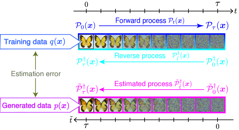
Figure 1: Illustration of the diffusion models in the case of image data. The forward process, denoted by $\mathcal{P}_{t}(\bm{x})$, is a stochastic process for adding noise to the training data sampled from $q(\bm{x})$. By inverting this forward process in time, we prepare the reverse process $\mathcal{P}^{\dagger}_{\tilde{t}}(\bm{x})$. The generated data sampled from $p(\bm{x})$ is constructed by an estimated process $\tilde{\mathcal{P}}^{\dagger}_{\tilde{t}}(\bm{x})$ that mimics the reverse process. The image in the figure is taken from the data set [91].

Specifically, the input probability density function $\mathcal{P}_{0}(\bm{x})=q(\bm{x})$ is transformed into a known noise distribution $\mathcal{P}_{\tau}(\bm{x})$ by adding noise to the input data, where $\mathcal{P}_{t}(\bm{x})$ is the probability density function at time $t\in[0,\tau]$. The time evolution of $\mathcal{P}_{t}(\bm{x})$ is given by the diffusion processes described by the Fokker-Planck equation [92] or the master equation [93] in the diffusion models [36, 35]. Sometimes we consider the stochastic dynamics of the data [36] from the initial state $\bm{x}_{t=0}$ to the final state $\bm{x}_{t=\tau}$ where $\bm{x}_{t}$ is the state of the data at time $t$ instead of the time evolution of the probability density function $\mathcal{P}_{t}(\bm{x})$. In this case, the stochastic time evolution of $\bm{x}_{t}$ can be described by the Langevin equation [1] or the Markov chain Monte Carlo (MCMC) method [94, 95, 96]. The diffusion process from $t=0$ to $t=\tau$ is called the forward process [35], and the dependence of the noise intensity at time $t$ in the forward process is called the noise schedule, which characterizes the time evolution of the diffusion dynamics [35, 43, 97].

Next, we will explain the reverse process, which is the time-reversed dynamics of the forward process. Here, we consider the forward process described by the time evolution of the probability density function $\mathcal{P}_{t}(\bm{x})$. We write the reverse process as $\mathcal{P}^{\dagger}_{\tilde{t}}(\bm{x})$, defined as $\mathcal{P}^{\dagger}_{\tilde{t}}(\bm{x})\coloneqq\mathcal{P}_{\tau-\tilde{t}}(\bm{x})$. In the reverse process, we consider the time evolution from $\tilde{t}=0$ to $\tilde{t}=\tau$. If $\tau$ is large enough, the final probability of the forward process $\mathcal{P}_{\tau}(\bm{x})$ can be considered as a noisy state where the data structure is well broken. Thus, the reverse process means that this noisy state $\mathcal{P}_{0}^{\dagger}(\bm{x})=\mathcal{P}_{\tau}(\bm{x})$ is the initial probability density function at time $\tilde{t}=0$ in the reverse process, and the time evolution in the reverse process allows the reproduction of the input data distribution $\mathcal{P}^{\dagger}_{\tau}(\bm{x})=\mathcal{P}_{0}(\bm{x})=q(\bm{x})$ containing the data structure at the final time $\tilde{t}=\tau$.

We introduce the stochastic process for generating the data from $p(\bm{x})$, namely the estimated process, as an imitation of the reverse process. This estimated process may differ from the reverse process in general, and so we write it as $\tilde{\mathcal{P}}^{\dagger}_{\tilde{t}}(\bm{x})$ and distinguish it from the reverse process $\mathcal{P}_{\tilde{t}}^{\dagger}(\bm{x})(\neq\tilde{\mathcal{P}}_{\tilde{t}}^{\dagger}(\bm{x}))$. Since the initial probability density function of the estimated process $\tilde{\mathcal{P}}_{0}^{\dagger}(\bm{x})$ can be different from the initial probability density function of the reverse process $\mathcal{P}_{0}^{\dagger}(\bm{x})(\neq\tilde{\mathcal{P}}_{0}^{\dagger}(\bm{x}))$, the final probability density function of the estimated process $\tilde{\mathcal{P}}^{\dagger}_{\tau}(\bm{x})$ can be different from the input distribution $q(\bm{x})(\neq\tilde{\mathcal{P}}^{\dagger}_{\tau}(\bm{x}))$. Here, the idea of diffusion models is to set this probability density function $\tilde{\mathcal{P}}_{\tau}^{\dagger}(\bm{x})$, which is the output of the estimated process, as the generated data distribution $p(\bm{x})$ [35]. In practical diffusion models, we do not necessarily compute the time evolution of the probability density function. For example, there are several methods to generate the data from the estimated process using the Langevin equation [42, 36] or the deterministic time evolution via flow [63]..

II.3 Fokker–Planck equation for the forward process

We discuss the time evolution of $\mathcal{P}_{t}(\bm{x})$ for the forward process in the diffusion models [36] based on the Fokker–Planck equation [92]. The time evolution of the probability density function $\mathcal{P}_{t}(\bm{x})$ is described by the Fokker–Planck equation as follows.

$$\partial_{t}\mathcal{P}_{t}(\bm{x}) =-\nabla\cdot\left(\bm{\nu}_{t}^{\mathcal{P}}(\bm{x})\mathcal{P}_{t}(\bm{x})\right),$$

$$\bm{\nu}_{t}^{\mathcal{P}}(\bm{x}) \coloneqq\bm{f}_{t}(\bm{x})-T_{t}\nabla\ln\mathcal{P}_{t}(\bm{x}),$$ (1)

where $\partial_{t}\coloneqq\partial/\partial t$ is the partial differential operator and $\nabla$ is the del operator. $\bm{\nu}^{\mathcal{P}}_{t}(\bm{x})\in\mathbb{R}^{n_{\rm d}}$ is the velocity field in a continuous equation. The parameters $T_{t}\in\mathbb{R}_{\geq 0}$ and $\bm{f}_{t}(\bm{x})\in\mathbb{R}^{n_{\rm d}}$ are functions of the time $t$ in general. The forward process can be regarded as the time evolution of $\mathcal{P}_{t}(\bm{x})$ by the Fokker–Planck equation [Eq. (1)] under the initial condition $\mathcal{P}_{0}(\bm{x})=q(\bm{x})$ with fixed time dependence of the parameters $T_{t}$ and $\bm{f}_{t}(\bm{x})$. The time dependence of $T_{t}$ characterizes the time variation of the noise intensity in the diffusion process, which is known as the noise schedule in the diffusion models.

The Fokker–Planck equation [Eq. (1)] is statistically equivalent to the stochastic differential equation, namely the Langevin equation [92, 93] for the state $\bm{x}_{t}$,

$$d\bm{x}_{t}=\bm{f}_{t}(\bm{x}_{t})dt+\sqrt{2T_{t}}dB_{t},$$ (2)

where $dB_{t}=B_{t+dt}-B_{t}$ is the random white Gaussian noise, mathematically defined as the difference of the Wiener processes $B_{t}$. If the Langevin equation is considered as Brownian dynamics for the position of a Brownian particle, the parameters $T_{t}$ and $\bm{f}_{t}(\bm{x}_{t})$ correspond to the temperature and the external force, respectively [92]. In the context of diffusion models, the forward process described by the Langevin equation can be viewed as a time-evolving process in which the random noise is sequentially added to the data. Using the Langevin equation, the time evolution of the forward process is calculated using the input data $\bm{x}^{(n)}\in d_{\mathrm{in}}$ $(n=1,\dots,N_{\rm D})$ for fixed time dependence of the parameters $T_{t}$ and $\bm{f}_{t}(\bm{x}_{t})$. The time evolution of the probability density function $\mathcal{P}_{t}(\bm{x})$ can be calculated numerically by Monte Carlo sampling using Langevin dynamics [96].

II.4 Reverse and estimated process

Next, we discuss the reverse process by considering the time-reversed dynamics of the Fokker-Planck equation for the forward process [Eq. (1)]. Using the reversed time $\tilde{t}=\tau-t$, the time evolution of $\mathcal{P}^{\dagger}_{\tilde{t}}(\bm{x})=\mathcal{P}_{\tau-\tilde{t}}(\bm{x})=\mathcal{P}_{t}(\bm{x})$ is given by the Fokker–Planck equation for the forward process [Eq. (1)] as follows,

$$\partial_{\tilde{t}}\mathcal{P}_{\tilde{t}}^{\dagger}(\bm{x}) =-\partial_{t}\mathcal{P}_{t}(\bm{x})$$

$$=\nabla\cdot\left(\bm{\nu}_{t}^{\mathcal{P}}(\bm{x})\mathcal{P}_{t}(\bm{x})\right)$$

$$=-\nabla\cdot\left(\bm{\nu}_{\tilde{t}}^{\dagger}(\bm{x})\mathcal{P}_{\tilde{t}}^{\dagger}(\bm{x})\right),$$ (3)

where the velocity field for the reverse process $\bm{\nu}_{\tilde{t}}^{\dagger}(\bm{x})$ is defined as ${\bm{\nu}_{\tilde{t}}^{\dagger}(\bm{x})\coloneqq-\bm{\nu}^{\mathcal{P}}_{\tau-\tilde{t}}}(\bm{x})$.

The diffusion models are introduced by the estimated process that mimics the reverse process [Eq. (3)]. We denote the probability density function of the data $\bm{x}$ in the estimated process by $\tilde{\mathcal{P}}^{\dagger}_{\tilde{t}}(\bm{x})$. We assume that the time evolution of this probability density function $\tilde{\mathcal{P}}^{\dagger}_{\tilde{t}}(\bm{x})$ can be written by the continuity equation,

$$\partial_{\tilde{t}}\tilde{\mathcal{P}}^{\dagger}_{\tilde{t}}(\bm{x})=-\nabla\cdot\left(\tilde{\bm{\nu}}_{\tilde{t}}^{\dagger}(\bm{x})\tilde{\mathcal{P}}_{\tilde{t}}^{\dagger}(\bm{x})\right).$$ (4)

Here, $\tilde{\bm{\nu}}_{\tilde{t}}^{\dagger}(\bm{x})$ represents the velocity field in the estimated process, which may differ from that of the reverse process ${\bm{\nu}}_{\tilde{t}}^{\dagger}(\bm{x})$. The velocity field $\tilde{\bm{\nu}}_{\tilde{t}}^{\dagger}(\bm{x})$ is estimated numerically from the dynamics of the forward process.

In the following section, we will explain two methods for estimating the velocity field in the reverse process and constructing the velocity field of the estimated process $\tilde{\bm{\nu}}_{\tilde{t}}^{\dagger}(\bm{x})$ for data generation, called the score-based generative modeling [42] and the flow-based generative modeling [63].

Example 1: Score-based generative modeling

First, we explain a method called score-based generative modeling [42]. This method consists of two components, score matching [56, 57, 58, 42] and data generation. Score matching is a method that estimates the score function $\nabla\ln\mathcal{P}_{t}(\bm{x})$ in the forward process [Eq. (1)] in order to arrange the estimated process [42, 36]. The score function is typically estimated using neural networks. Specifically, we consider a situation where the score function $\nabla\ln\mathcal{P}_{t}(\bm{x})$ is modeled by a neural network denoted by $\bm{s}^{\theta}_{t}(\bm{x})$ where $\theta$ represents the set of the network’s parameters. We then solve an optimization problem numerically to estimate the score function. The optimized parameters, denoted by $\theta^{*}_{\rm{SM}}$, are employed to generate the velocity field of the estimated process $\tilde{\bm{\nu}}_{\tilde{t}}^{\dagger}(\bm{x})$.

The optimization problem is constructed as follows. The optimization problem to estimate the score function $\nabla\ln\mathcal{P}_{t}(\bm{x})$ is formulated as a minimization problem of the following score matching objective function.

$$L_{\rm SM}(\theta)=\mathbb{E}_{\mathcal{P}_{t},\mathcal{U}}\left[\|\bm{s}^{\theta}_{t}(\bm{x})-\nabla\ln\mathcal{P}_{t}(\bm{x})\|^{2}\right].$$ (5)

Here, the uniform distribution for $t\in[0,\tau]$ is given by $\mathcal{U}(t)=1/\tau$. The expected value with respect to this uniform distribution and the distribution $\mathcal{P}_{t}(\bm{x})$ is defined as $\mathbb{E}_{\mathcal{P}_{t},\mathcal{U}}\left[\cdots\right]=\int_{0}^{\tau}dt\mathcal{U}(t)\int d\bm{x}\mathcal{P}_{t}(\bm{x})\cdots$. Then, the optimal set of the parameters $\theta^{*}_{\rm{SM}}$ is obtained as [57, 36],

$$\theta^{*}_{\rm SM}\in{\rm argmin}_{\theta}L_{\rm SM}(\theta).$$ (6)

In this optimization problem, $\bm{s}^{\theta^{*}_{\rm SM}}_{t}(\bm{x})$, which reaches the minimum value $L_{\rm SM}(\theta^{*}_{\rm SM})=0$, can be the score function $\nabla\ln\mathcal{P}_{t}(\bm{x})$.

Example 1-1: Stochastic differential equation

For the data generation by the estimated process, we first explain the method based on the stochastic differential equations [36, 42, 40]. The estimated score function, $\bm{s}^{\theta^{*}_{\rm SM}}_{t}(\bm{x})$, is employed to reconstruct the velocity field of the forward process $\bm{\nu}_{t}^{\mathcal{P}}(\bm{x})$ as,

$$\hat{\bm{\nu}}_{t}(\bm{x})\coloneqq\bm{f}_{t}(\bm{x})-T_{t}{\bm{s}}^{\theta^{*}_{\rm SM}}_{t}(\bm{x}).$$ (7)

With this estimated velocity field $\hat{\bm{\nu}}_{t}(\bm{x})$, we construct the velocity field of the estimated process $\tilde{\bm{\nu}}_{\tilde{t}}^{\dagger}(\bm{x})$ as

$$\tilde{\bm{\nu}}_{\tilde{t}}^{\dagger}(\bm{x}) =[\bm{\nu}_{\tilde{t}}^{\tilde{\mathcal{P}}^{\dagger}}(\bm{x})]^{\dagger}-2\hat{\bm{\nu}}_{\tau-\tilde{t}}(\bm{x})$$

$$=-\bm{f}_{\tilde{t}}^{\dagger}(\bm{x})+2T_{\tilde{t}}^{\dagger}{\bm{s}}^{\theta^{*}_{\rm SM}\dagger}_{\tilde{t}}(\bm{x})-T_{\tilde{t}}^{\dagger}\nabla\ln\tilde{\mathcal{P}}_{\tilde{t}}^{\dagger}(\bm{x}),$$ (8)

so that the estimated process [Eq. (4)] mimics the reverse process [Eq. (3)], where $[\bm{\nu}_{\tilde{t}}^{\tilde{\mathcal{P}}^{\dagger}}(\bm{x})]^{\dagger}\coloneqq\bm{f}_{\tilde{t}}^{\dagger}(\bm{x})-T_{\tilde{t}}^{\dagger}\nabla\ln\tilde{\mathcal{P}}_{\tilde{t}}^{\dagger}(\bm{x})$, $\bm{f}_{\tilde{t}}^{\dagger}(\bm{x})\coloneqq\bm{f}_{\tau-\tilde{t}}(\bm{x})$, $T_{\tilde{t}}^{\dagger}\coloneqq T_{\tau-\tilde{t}}$, and ${\bm{s}}^{\theta^{*}_{\rm SM}\dagger}_{\tilde{t}}(\bm{x})\coloneqq{\bm{s}}^{\theta^{*}_{\rm SM}}_{\tau-\tilde{t}}(\bm{x})$. If ${\bm{s}}^{\theta^{*}_{\rm SM}}_{t}(\bm{x})$ is exactly equal to $\nabla\ln\mathcal{P}_{t}(\bm{x})$ and the initial condition for the estimated process is equivalent to the initial condition for the reverse process ($\tilde{\mathcal{P}}_{0}^{\dagger}(\bm{x})=\mathcal{P}_{0}^{\dagger}(\bm{x})$), the equation $\tilde{\bm{\nu}}_{\tilde{t}}^{\dagger}(\bm{x})=\bm{\nu}_{\tilde{t}}^{\dagger}(\bm{x})$ holds and the reverse process [Eq. (3)] is consistent with the estimated process [Eq. (4)].

The continuity equation of the estimated process $\partial_{\tilde{t}}\tilde{\mathcal{P}}^{\dagger}_{\tilde{t}}(\bm{x})=-\nabla\cdot\left(\tilde{\bm{\nu}}_{\tilde{t}}^{\dagger}(\bm{x})\tilde{\mathcal{P}}_{\tilde{t}}^{\dagger}(\bm{x})\right)$ using the estimated velocity field $\tilde{\bm{\nu}}^{\dagger}_{\tilde{t}}(\bm{x})$ can be regarded as the Fokker–Planck equation with the external force $-\bm{f}^{\dagger}_{\tilde{t}}(\bm{x})+2T^{\dagger}_{\tilde{t}}{\bm{s}}^{\theta^{*}_{\rm SM}\dagger}_{\tilde{t}}(\bm{x})$. The stochastic differential equation, (i.e., Langevin equation) corresponding to this Fokker–Planck equation is [36, 98],

$$d\tilde{\bm{x}}^{\dagger}_{\tilde{t}}=\left(-\bm{f}_{\tilde{t}}^{\dagger}(\tilde{\bm{x}}^{\dagger}_{\tilde{t}})+2T^{\dagger}_{\tilde{t}}{\bm{s}}^{\theta^{*}_{\rm SM}\dagger}_{\tilde{t}}(\tilde{\bm{x}}^{\dagger}_{\tilde{t}})\right)d\tilde{t}+\sqrt{2T_{\tilde{t}}^{\dagger}}d{B}_{\tilde{t}},$$ (9)

where $d{B}_{\tilde{t}}={B}_{\tilde{t}+d\tilde{t}}-{B}_{\tilde{t}}$ is the difference of the Wiener process $B_{\tilde{t}}$ and $\tilde{\bm{x}}^{\dagger}_{\tilde{t}}$ is the state of the data in the estimated process. By simulating this stochastic differential equation numerically, we can generate the data in score-based generative modeling [36, 42, 40].

Example 1-2: Probability flow ordinary differential equation

Next, we discuss an alternative method for data generation in score-based generative modeling, namely the probability flow ordinary differential equation (ODE) [36]. The probability flow ODE is a method in which we use an ODE instead of the stochastic differential equation [Eq. (9)] for data generation under the same objective function [Eq. (5)]. At present, this probability flow ODE is well used instead of the stochastic differential equation because it is possible to generate data faster and more accurately by performing time evolution based on numerical ODE solvers [99, 100, 101].

Specifically, using the velocity field $\hat{\bm{\nu}}_{t}(\bm{x})$ [Eq. (7)] estimated through the objective function [Eq. (5)], the velocity field of the estimated process $\tilde{\bm{\nu}}^{\dagger}_{\tilde{t}}(\bm{x})$ is arranged as follows.

$$\tilde{\bm{\nu}}^{\dagger}_{\tilde{t}}(\bm{x})=-\hat{\bm{\nu}}_{\tau-\tilde{t}}(\bm{x}).$$ (10)

This expression is parallel to the expression of the velocity field in the reverse process $\bm{\nu}_{\tilde{t}}^{\dagger}(\bm{x})=-\bm{\nu}_{\tau-\tilde{t}}^{\mathcal{P}}(\bm{x})$. In this case, the continuity equation [Eq. (4)] corresponds to the following ODE [36, 61].

$$\frac{d\tilde{\bm{x}}_{\tilde{t}}^{\dagger}}{d\tilde{t}}=-\hat{\bm{\nu}}_{\tau-\tilde{t}}(\tilde{\bm{x}}_{\tilde{t}}^{\dagger})=-\bm{f}^{\dagger}_{\tilde{t}}(\tilde{\bm{x}}^{\dagger}_{\tilde{t}})+T^{\dagger}_{\tilde{t}}{\bm{s}}^{\theta^{*}_{\rm SM}\dagger}_{\tilde{t}}(\tilde{\bm{x}}^{\dagger}_{\tilde{t}}),$$ (11)

where $\tilde{\bm{x}}^{\dagger}_{\tilde{t}}$ denotes the sample from $\tilde{\mathcal{P}}^{\dagger}_{\tilde{t}}(\bm{x})$. The probability flow ODE method generates data by numerically simulating this ODE [36].

Example 2: Flow-based generative modeling

Next, we explain the flow-based generative modeling [63] which consists of flow matching and data generation via the ODE. Flow matching [63] is a method to estimate the velocity field of the forward process without estimating the score function. In flow matching, we model the velocity field of the forward process $\bm{\nu}_{t}^{\mathcal{P}}(\bm{x})$ by a neural network $\bm{u}_{t}^{\theta}\in\mathbb{R}^{n_{\rm d}}$ where $\theta$ is the set of parameters. The objective function,

$$L_{\rm FM}(\theta)=\mathbb{E}_{\mathcal{P}_{t},\mathcal{U}}\left[\|\bm{u}_{t}^{\theta}(\bm{x})-\bm{\nu}^{\mathcal{P}}_{t}(\bm{x})\|^{2}\right],$$ (12)

is minimized with respect to $\theta$ using numerical optimization methods, and $\theta^{*}_{\rm FM}$ is the optimal set of the parameters satisfying

$$\theta^{*}_{\rm FM}\in\operatorname{argmin}_{\theta}L_{\rm FM}(\theta).$$ (13)

The optimal set of the parameters $\theta^{*}_{\rm FM}$ gives the velocity field for the estimated process $\tilde{\bm{\nu}}^{\dagger}_{\tilde{t}}(\bm{x})$ as follows,

$$\tilde{\bm{\nu}}^{\dagger}_{\tilde{t}}(\bm{x})=-{\bm{u}}_{\tau-\tilde{t}}^{\theta^{*}_{\rm FM}}(\bm{x}).$$ (14)

This expression corresponds to the velocity field of the reverse process $\bm{\nu}^{\dagger}_{\tilde{t}}(\bm{x})=-\bm{\nu}_{\tau-\tilde{t}}^{\mathcal{P}}(\bm{x})$.

In the flow-based generative modeling, the data generation is done by simulating the ODE [63, 102],

$$\frac{d\tilde{\bm{x}}_{\tilde{t}}^{\dagger}}{d\tilde{t}}=-{\bm{u}}_{\tau-\tilde{t}}^{\theta^{*}_{\rm FM}}(\tilde{\bm{x}}_{\tilde{t}}^{\dagger}),$$ (15)

which is similar to that used in the probability flow ODE method [Eq. (11)]. This ODE corresponds to the continuity equation for the estimated process [Eq. (4)].

II.5 Formulations with conditional Gaussian distributions

In a practical implementation of the diffusion models, we may consider a process such that the external force $\bm{f}_{t}(\bm{x})$ is linear,

$$\bm{f}_{t}(\bm{x})=\mathsf{A}_{t}\bm{x}+\bm{b}_{t},$$ (16)

to reduce the computational complexity [35, 36, 40, 42, 63], where $\mathsf{A}_{t}\in\mathbb{R}^{n_{\rm d}\times n_{\rm d}}$ and $\bm{b}_{t}\in\mathbb{R}^{n_{\rm d}}$ are the matrix and the vector, respectively. When the initial condition is $\mathcal{P}_{t=0}(\bm{x})=q(\bm{x})$, the solution $\mathcal{P}_{t}(\bm{x})$ for the process can be given by

$$\mathcal{P}_{t}(\bm{x})=\int\mathcal{P}^{\rm c}_{t}(\bm{x}|\bm{y})q(\bm{y})d\bm{y}.$$ (17)

Here, the transition probability $\mathcal{P}^{\rm c}_{t}(\bm{x}|\bm{y})$ is a Gaussian distribution $\mathcal{P}^{\rm c}_{t}(\bm{x}|\bm{y})=\mathcal{N}(\bm{x}|\bm{\mu}_{t}(\bm{y}),\mathsf{\Sigma}_{t})$ due to the linearity of the external force [92], where $\bm{\mu}_{t}(\bm{y})$ is the mean, which depends on $\bm{y}$, and $\mathsf{\Sigma}_{t}$ is the covariance matrix $\mathsf{\Sigma}_{t}$. We assume that $\mathsf{\Sigma}_{t}$ does not depend on the state $\bm{y}$. The equation (17) at $t=0$ gives the condition $\mathcal{P}^{\rm c}_{0}(\bm{x}|\bm{y})=\delta(\bm{x}-\bm{y})$, where $\delta(\bm{x}-\bm{y})$ is the delta function. Thus, the covariance matrix at $t=0$ is $\mathsf{\Sigma}_{t=0}=\mathsf{O}$, and the mean is $\bm{\mu}_{t=0}(\bm{y})=\bm{y}$, where $\mathsf{O}$ is the zero matrix.

Under the above condition, the optimization problems [Eqs. (5), (12)] are easier to solve [63, 42]. These training methods using conditional probability in score matching and flow matching are known as denoising score matching [57] and conditional flow matching [63], respectively. To reduce the computational complexity, we consider new objective functions, which correspond to the objective functions [Eqs. (5), (12)] as follows,

$$L_{\rm SM}^{\rm c}(\theta)=\mathbb{E}_{\mathcal{P}^{\rm c}_{t},q,\mathcal{U}}\left[\|\bm{s}^{\theta}_{t}(\bm{x})-\nabla\ln\mathcal{P}^{\rm c}_{t}(\bm{x}|\bm{y})\|^{2}\right],$$ (18)

$$L_{\rm FM}^{\rm c}(\theta)=\mathbb{E}_{\mathcal{P}^{\rm c}_{t},q,\mathcal{U}}\left[\|\bm{u}_{t}^{\theta}(\bm{x})-\bm{\nu}^{\mathcal{P}^{\rm c}}_{t}(\bm{x}|\bm{y})\|^{2}\right],$$ (19)

where $\mathbb{E}_{\mathcal{P}^{\rm c}_{t},q,\mathcal{U}}\left[\cdots\right]=\int_{0}^{\tau}dt\mathcal{U}(t)\int d\bm{x}d\bm{y}\mathcal{P}^{\rm c}_{t}(\bm{x}|\bm{y})q(\bm{y})\cdots$ is the expected value with respect to $\mathcal{P}^{\rm c}_{t}(\bm{x}|\bm{y})$, $q(\bm{y})$, and $\mathcal{U}(t)$, and $\bm{\nu}_{t}^{\mathcal{P}^{\rm c}}(\bm{x}|\bm{y})\coloneqq\bm{f}_{t}(\bm{x})-T_{t}\nabla\ln\mathcal{P}^{\rm c}_{t}(\bm{x}|\bm{y})$. As proved in Appendix A, new objective functions satisfy $\nabla_{\theta}L_{\rm SM}^{\rm c}(\theta)=\nabla_{\theta}L_{\rm SM}(\theta)$ and $\nabla_{\theta}L_{\rm FM}^{\rm c}(\theta)=\nabla_{\theta}L_{\rm FM}(\theta)$, where $\nabla_{\theta}$ is the gradient through $\theta$. Since the optimal solutions are given by the conditions $\nabla_{\theta}L_{\rm SM}^{\rm c}(\theta)=\nabla_{\theta}L_{\rm SM}(\theta)=0$ and $\nabla_{\theta}L_{\rm FM}^{\rm c}(\theta)=\nabla_{\theta}L_{\rm FM}(\theta)=0$, we get the optimal solutions,

$$\theta^{*}_{\rm SM} \in\operatorname{argmin}_{\theta}L_{\rm SM}^{\rm c}(\theta),$$ (20)

$$\theta^{*}_{\rm FM} \in\operatorname{argmin}_{\theta}L_{\rm FM}^{\rm c}(\theta),$$ (21)

which are equivalent to the solutions of the original problems [Eqs. (6) and (13)]. Here, the quantities $\nabla\ln\mathcal{P}^{\rm c}_{t}(\bm{x}|\bm{y})$ and $\bm{\nu}^{\mathcal{P}^{\rm c}}_{t}(\bm{x}|\bm{y})$ are linear functions of $\bm{x}$ because of the Gaussian property, and the conditional probability $\mathcal{P}^{\rm c}_{t}(\bm{x}|\bm{y})$ can be sampled more easily than $\mathcal{P}_{t}(\bm{x})$ due to the reproductive property of Gaussian distributions. Therefore, these optimization problems [Eqs. (18) and (19)] are numerically simpler than the original optimization problems [Eqs. (5) and (12)].

II.6 Examples of diffusion models

We present some representative examples of existing diffusion models [43, 48, 63, 40]. Here we discuss the conditional Gaussian formulations from the previous section. We consider the temperature $T_{t}$ and the external force $\bm{f}_{t}(\bm{x})$ as functions of non-negative parameters $\sigma_{t}(\geq 0)$, $m_{t}(\geq 0)$ such that

$$T_{t}=m_{t}\sigma_{t}\partial_{t}\left(\frac{\sigma_{t}}{m_{t}}\right)=\partial_{t}\left(\frac{\sigma_{t}^{2}}{2}\right)-\sigma_{t}^{2}\partial_{t}\ln m_{t},$$ (22)

$$\bm{f}_{t}(\bm{x})=\nabla\left(\frac{\partial_{t}\ln m_{t}}{2}\left\|\bm{x}\right\|^{2}\right)=(\partial_{t}\ln m_{t})\bm{x}.$$ (23)

The external force $\bm{f}_{t}(\bm{x})$ is described by the linear function [Eq. (16)] with $\mathsf{A}_{t}=(\partial_{t}\ln m_{t})\mathsf{I}$, $\bm{b}_{t}=\bm{0}$, where $\mathsf{I}$ is the identity matrix and $\bm{0}$ is the zero vector. The time dependence of $m_{t}$ and $\sigma_{t}$ is also called the noise schedule [43, 48, 63, 40] because the diffusion dynamics can be determined by the time dependence of $m_{t}$ and $\sigma_{t}$ instead of the time dependence of $T_{t}$ and $\bm{f}_{t}(\bm{x})$.

We sometimes make the following assumption for the noise schedules. To satisfy $T_{t}\geq 0$, the monotony condition

$$\begin{split}\partial_{t}\left(\frac{\sigma_{t}}{m_{t}}\right)\geq 0,\end{split}$$ (24)

is assumed. The term $m_{t}/\sigma_{t}$ is called the signal-to-noise ratio [41], which must be monotonically non-increasing. Furthermore, we assume the initial conditions $m_{t=0}=1$ and $\sigma_{t=0}=0$. Under these initial conditions, the solutions of the mean $\bm{\mu}_{t}(\bm{y})$ and the covariance matrix $\mathsf{\Sigma}_{t}$ in $\mathcal{P}^{\rm c}_{t}(\bm{x}|\bm{y})$ are given by

$$\bm{\mu}_{t}(\bm{y})=m_{t}\bm{y},\>\>\mathsf{\Sigma}_{t}=\sigma_{t}^{2}\mathsf{I},$$ (25)

[see Appendix B]. For high-dimensional data sets such as images, we often use this assumption [40, 48, 63, 36]. In the following, we show some examples of the noise schedules.

Example 1: Variance exploding diffusion (VE-diffusion)

We first introduce the variance exploding diffusion (VE-diffusion) [36]. The VE-diffusion is a method based on the noise conditional score networks (NCSN) [42], which is described by the following Langevin equation [36]

$$d\bm{x}_{t}=\sqrt{2T_{t}}dB_{t}.$$ (26)

This equation corresponds to the condition that there is no external force $\bm{f}_{t}(\bm{x})=\bm{0}$. From Eqs. (22) and (23), we obtain $\partial_{t}\ln m_{t}=0$ and

$$T_{t}=\partial_{t}\left(\frac{\sigma_{t}^{2}}{2}\right).$$ (27)

The condition $\partial_{t}\ln m_{t}=0$ means that the noise schedule is given by $m_{t}=1\>(0\leq t\leq\tau)$ because the initial condition is given by $m_{0}=1$. Because of Eq. (24), $\sigma_{t}$ should be a monotonically non-decreasing function of time. While we explain the VE-diffusion in terms of the Langevin equation, this method can be described in the implementation as the probabilistic flow ODE.

Example 2: Optimal transport conditional flow matching

Next, we introduce the conditional optimal transport (cond-OT) schedule used in flow matching. The cond-OT schedule is known as a noise schedule that optimizes the transport of the conditional distribution $\mathcal{P}_{t}^{\rm c}(\bm{x}|\bm{y})$ [63], which is described as follows,

$$\begin{split}&m_{t}=1-\frac{t}{\tau},\\ &\sigma_{t}=\frac{t}{\tau}.\end{split}$$ (28)

This noise schedule represents the change of the parameters along the geodesic from $(\sigma_{t},m_{t})=(0,1)$ to $(\sigma_{t},m_{t})=(1,0)$ on the $2$-dimensional Euclidean space of the standard deviation $\sigma_{t}$ and the mean $m_{t}$. The dynamics along the geodesic can be regarded as optimal transport based on the $2$-Wasserstein distance for the conditional probability distributions [63, 70].

Example 3: Variance Preserving diffusion (VP-diffusion)

Finally, we introduce the variance preserving diffusion (VP-diffusion) [36]. The VP-diffusion is a method based on the denoising diffusion probabilistic model (DDPM) [43]. The DDPM is a diffusion model that uses the diffusion from the input data distribution to the Gaussian distribution $\mathcal{N}(\bm{x}|\bm{0},\mathsf{I})$. The VP-diffusion is described by the following Langevin equation [36],

$$d\bm{x}_{t}=-T_{t}\bm{x}_{t}dt+\sqrt{2T_{t}}dB_{t}.$$ (29)

From Eq. (2) and (23) we get $\bm{f}_{t}(\bm{x})=-T_{t}\bm{x}$ and $\partial_{t}\ln m_{t}=-T_{t}$. By substituting $\partial_{t}\ln m_{t}=-T_{t}$ for Eq. (22), we also obtain the relation

$$\partial_{t}\ln(m_{t}^{2})=\frac{\partial_{t}(\sigma_{t}^{2})}{\sigma_{t}^{2}-1}=\partial_{t}\ln(1-\sigma^{2}_{t}).$$ (30)

Since the initial conditions are given by $\sigma_{0}=0$ and $m_{0}=1$, the condition

$$m_{t}^{2}+\sigma_{t}^{2}=1,$$ (31)

holds. This condition implies that $m_{t}$ and $\sigma_{t}$ are on the unit circle. Thus, we can consider a noise schedule that changes the parameters along the geodesic on the unit circle from $(\sigma_{t},m_{t})=(0,1)$ to $(\sigma_{t},m_{t})=(1,0)$ as follows,

$$\begin{split}&m_{t}=\cos\left(\frac{\pi}{2}\frac{t}{\tau}\right),\\ &\sigma_{t}=\sin\left(\frac{\pi}{2}\frac{t}{\tau}\right).\end{split}$$ (32)

This noise schedule is called the cosine schedule [43].

Under the condition of the VP-diffusion ($\sigma_{t}^{2}+m_{t}^{2}=1$), we consider the coordinate transformation to treat the diffusion process without the external force. The method based on the coordinate transformation is called the denoising diffusion implicit model (DDIM) [48]. The coordinate transformation in the DDIM is introduced as follows,

$$\bar{\bm{x}}=\frac{\bm{x}}{m_{t}}.$$ (33)

Under this coordinate transformation, the conditions Eq. (22) with $T_{t}=-\partial_{t}\ln m_{t}$, the Fokker-Planck equation is given by

$$\partial_{t}\bar{\mathcal{P}}_{t}(\bar{\bm{x}})=-\nabla_{\bar{\bm{x}}}\cdot\left[\left[\frac{\partial_{t}\ln m_{t}}{(m_{t})^{2}}\nabla_{\bar{\bm{x}}}\ln\bar{\mathcal{P}}_{t}(\bar{\bm{x}})\right]\bar{\mathcal{P}}_{t}(\bar{\bm{x}})\right],$$ (34)

(see Appendix C), where $\bar{\mathcal{P}}_{t}(\bar{\bm{x}})\coloneqq\mathcal{P}_{t}(\bm{x})(|d\bar{\bm{x}}/d\bm{x}|)^{-1}$, $\nabla_{\bar{\bm{x}}}\coloneqq m_{t}\nabla$, and $|d\bar{\bm{x}}/d\bm{x}|$ is the Jacobian. Therefore, the corresponding Langevin equation is

$$d\bar{\bm{x}}_{t}=\sqrt{\frac{2T_{t}}{(m_{t})^{2}}}dB_{t}.$$ (35)

This Langevin equation describes a situation where the external force is absent. In the DDIM, we generate data using the probability flow ODE [Eq. (11)] [48].

III Relationships between stochastic thermodynamics and diffusion models

In this section, we review stochastic thermodynamics (Sec. III.1) and the relationship between stochastic thermodynamics and optimal transport theory (Sec. III.2) from the perspective of diffusion models.

III.1 Review on stochastic thermodynamics

We introduce nonequilibrium thermodynamics for the overdamped Fokker–Planck equation [Eq. (1)], namely stochastic thermodynamics [3], and discuss its relation to the diffusion models. In stochastic thermodynamics, we mainly consider the quantity called the entropy production rate as a measure of thermodynamic dissipation rate. For the overdamped Fokker–Planck equation [Eq. (1)], the entropy production rate $\dot{S}^{\mathrm{tot}}_{t}$ is defined as

$$\dot{S}^{\mathrm{tot}}_{t} =\frac{1}{T_{t}}\int d\bm{x}\|\bm{\nu}_{t}^{\mathcal{P}}(\bm{x})\|^{2}\mathcal{P}_{t}(\bm{x}).$$ (36)

Here, the Boltzmann constant $k_{\rm B}$ is regularized to $k_{\rm B}=1$. This entropy production rate can be decomposed into the entropy change rate in the system $\dot{S}^{\mathrm{sys}}_{t}$ and the entropy change rate in the heat bath $\dot{S}^{\mathrm{bath}}_{t}$ as follows,

$$\dot{S}^{\mathrm{tot}}_{t}= \dot{S}^{\mathrm{sys}}_{t}+\dot{S}^{\mathrm{bath}}_{t},$$ (37)

$$\dot{S}^{\mathrm{sys}}_{t}= \partial_{t}\left[-\int d\bm{x}\mathcal{P}_{t}(\bm{x})\ln\mathcal{P}_{t}(\bm{x})\right],$$ (38)

$$\dot{S}^{\mathrm{bath}}_{t}= \frac{\int d\bm{x}\bm{f}_{t}(\bm{x})\cdot\bm{\nu}_{t}^{\mathcal{P}}(\bm{x})\mathcal{P}_{t}(\bm{x})}{T_{t}},$$ (39)

where we used the partial integration and $\int d\bm{x}\partial_{t}\mathcal{P}_{t}(\bm{x})=0$ to derive the expression $\dot{S}^{\mathrm{sys}}_{t}$. Thus, the entropy production rate $\dot{S}^{\mathrm{tot}}_{t}$ is regarded as the entropy change rate in the total system. Its non-negativity $\dot{S}^{\mathrm{tot}}_{t}\geq 0$ means the second law of thermodynamics. As a measure of thermodynamic dissipation, the entropy production from time $t=0$ to $t=\tau$ is also defined as

$${S}^{\mathrm{tot}}_{\tau}= \int_{0}^{\tau}dt\dot{S}^{\mathrm{tot}}_{t}.$$ (40)

In the original paper of the diffusion model [35], the idea of a reverse process in diffusion models may be inspired by the fluctuation theorem [37, 38, 8] or the Jarzynski equality [39], which are the relations between the entropy production and the path probabilities of the forward and backward trajectories. Based on mathematical techniques in the fluctuation theorem such as dual dynamics [3], we introduce the following dynamics

$$d\bm{x}_{t}=\bm{f}_{t}(\bm{x}_{t})dt-2\bm{\nu}_{t}^{\mathcal{P}}(\bm{x}_{t})dt+\sqrt{2T_{t}}dB_{t},$$ (41)

which corresponds to the estimated process of the score-based generative modeling [Eq. (9)] and is a special case of the interpolated dynamics [32] for the velocity field $-\bm{\nu}_{t}^{\mathcal{P}}(\bm{x}_{t})$.

Here, we discuss two path probabilities of the path $\Gamma=\{\bm{x}_{0},\bm{x}_{\Delta t},\cdots,\bm{x}_{N_{\tau}\Delta t}\}$. Here, $\Delta t(>0)$ is the infinitesimal time interval, and thus we consider the limit $\Delta t\to 0$ with fixed $\tau=N_{\tau}\Delta t$. For the Langevin equation [Eq. (2)], the transition probability from the state $\bm{x}$ at time $t$ to the state $\bm{y}$ at time $t+\Delta t$ is given by the expression of the Onsager–Machlup function [92] as follows,

$$\mathcal{T}_{t}(\bm{y}|\bm{x})=\frac{1}{(4\pi T_{t}\Delta t)^{\frac{n_{\rm d}}{2}}}e^{-\frac{\left\|\bm{y}-\bm{x}-\bm{f}_{t}(\bm{x})\Delta t\right\|^{2}}{4T_{t}\Delta t}}.$$ (42)

Similarly, the transition probability from the state $\bm{x}$ at time $t$ to the state $\bm{y}$ at time $t+\Delta t$ for the process [Eq. (41)] is given by

$$\mathcal{T}^{\dagger}_{t}(\bm{y}|\bm{x})=\frac{1}{(4\pi T_{t}\Delta t)^{\frac{n_{\rm d}}{2}}}e^{-\frac{\left\|\bm{y}-\bm{x}-\bm{f}_{t}(\bm{x})\Delta t+2\bm{\nu}^{\mathcal{P}}_{t}(\bm{x})\Delta t\right\|^{2}}{4T_{t}\Delta t}}.$$ (43)

Using the transition probability [Eq. (42)], we define the path probability for the forward process as

$$\mathbb{P}_{\rm F}(\Gamma)=\mathcal{P}_{0}(\bm{x}_{0})\prod_{N=0}^{N_{\tau}-1}\mathcal{T}_{N\Delta t}(\bm{x}_{(N+1)\Delta t}|\bm{x}_{N\Delta t}),$$ (44)

This path probability $\mathbb{P}_{\rm F}(\Gamma)$ is related to the distribution of the forward process $\mathcal{P}_{t}(\bm{x})$. If we consider the path excluding the state $\{\bm{x}_{n\Delta t}\}$ defined as $\Gamma_{t\neq n\Delta t}=\Gamma\setminus\{\bm{x}_{n\Delta t}\}$, marginalizing the path probability $\mathbb{P}_{\rm F}(\Gamma)$ gives $\mathcal{P}_{n\Delta t}(\bm{x}_{n\Delta t})=\int d\Gamma_{t\neq n\Delta t}\mathbb{P}_{\rm F}(\Gamma)$. Similarly, the path probability for the process in Eq. (41) is given by

$$\mathbb{P}_{\rm B}(\Gamma)=\mathcal{P}_{0}(\bm{x}_{0})\prod_{N=0}^{N_{\tau}-1}\mathcal{T}^{\dagger}_{N\Delta t}(\bm{x}_{(N+1)\Delta t}|\bm{x}_{N\Delta t}).$$ (45)

We remark that this path probability $\mathbb{P}_{\rm B}$ is not related to the reverse process or the estimated process, and marginalizing the path probability $\mathbb{P}_{\rm B}(\Gamma)$ does not yield $\mathcal{P}_{\tilde{t}}^{\dagger}(\bm{x})$ or $\tilde{\mathcal{P}}^{\dagger}_{\tilde{t}}(\bm{x})$ because this path probability $\mathbb{P}_{\rm B}$ is not introduced as the time-reversed dynamics from the probability distribution function ${\mathcal{P}}^{\dagger}_{0}$ or $\tilde{\mathcal{P}}^{\dagger}_{0}$.

The entropy production can be interpreted as the statistical difference between two path probabilities $\mathbb{P}_{\rm F}$ and $\mathbb{P}_{\rm B}$. If we consider the Kullback–Leibler divergence between $\mathbb{P}_{\rm F}(\Gamma)$ and $\mathbb{P}_{\rm B}(\Gamma)$ defined as

$$D_{\rm KL}(\mathbb{P}_{\rm F}\|\mathbb{P}_{\rm B})=\int d\Gamma\mathbb{P}_{\rm F}(\Gamma)\ln\frac{\mathbb{P}_{\rm F}(\Gamma)}{\mathbb{P}_{\rm B}(\Gamma)},$$ (46)

we obtain the following relation between the Kullback-Leibler divergence and the entropy production [3, 22, 32]

$${S}^{\mathrm{tot}}_{\tau}=D_{\rm KL}(\mathbb{P}_{\rm F}\|\mathbb{P}_{\rm B}),$$ (47)

(see also Appendix D).

We remark that there are several expressions of the entropy production as the Kullback-Leibler divergence. For example, the entropy production can be formulated as the projection in information geometry, which is a minimization problem of the Kullback-Leibler divergence [103, 32]. In the context of the fluctuation theorem, the expression based on the path probability for the backward trajectory is well discussed. The path probability for the backward trajectory is defined as

$$\mathbb{P}_{\rm B}^{\prime}(\Gamma)=\mathcal{P}_{\tau}(\bm{x}_{N_{\tau}\Delta t})\prod_{N=0}^{N_{\tau}-1}\mathcal{T}_{N\Delta t}(\bm{x}_{N\Delta t}|\bm{x}_{(N+1)\Delta t}).$$ (48)

We remark that this path probability $\mathbb{P}^{\prime}_{\rm B}$ is not related to the reverse process or the estimated process because this path probability $\mathbb{P}^{\prime}_{\rm B}$ uses the transition probability $\mathcal{T}_{t}$, which is not the transition probability of the reverse process or the estimated process, in the time-reversed dynamics from the initial condition ${\mathcal{P}}_{\tau}={\mathcal{P}}^{\dagger}_{0}$. We can also obtain the similar relation between the Kullback-Leibler divergence and the entropy production [104, 3, 32]

$${S}^{\mathrm{tot}}_{\tau}=D_{\rm KL}(\mathbb{P}_{\rm F}\|\mathbb{P}_{\rm B}^{\prime}),$$ (49)

(see also Appendix D). We here define the stochastic entropy production for the path $\Gamma$ as $s^{\rm tot}_{\tau}(\Gamma)=\ln[\mathbb{P}_{\rm F}(\Gamma)/\mathbb{P}_{\rm B}^{\prime}(\Gamma)]$. In stochastic thermodynamics, the identity $\exp[s^{\rm tot}_{\tau}(\Gamma)]=\mathbb{P}_{\rm F}(\Gamma)/\mathbb{P}_{\rm B}^{\prime}(\Gamma)$ is known as the detailed fluctuation theorem [37, 38, 8]. If we introduce the expected value with respect to $\mathbb{P}_{\rm F}$ as $\mathbb{E}_{\mathbb{P}_{\rm F}}[\cdots]=\int d\Gamma\mathbb{P}_{\rm F}(\Gamma)\cdots$, the entropy production satisfies $S^{\rm tot}_{\tau}=\mathbb{E}_{\mathbb{P}_{\rm F}}[s^{\rm tot}_{\tau}]$. We also can obtain the following identity

$$\mathbb{E}_{\mathbb{P}_{\rm F}}[\exp(-s^{\rm tot}_{\tau})]=1,$$ (50)

where we used the normalization $\int d\Gamma\mathbb{P}_{\rm B}^{\prime}(\Gamma)=1$, This formula is known as the integral fluctuation theorem [37, 38], and a special case of the integral fluctuation theorem is known as the Jarnzynski equality [39].

We remark on the analogous connection between the fluctuation theorem and the diffusion model discussed in the original paper on diffusion models [35]. In Ref. [35], the path probability for the estimated process $\mathbb{P}_{\rm E}$ is introduced as

$$\mathbb{P}_{\rm E}(\Gamma)=\tilde{\mathcal{P}}^{\dagger}_{0}(\bm{x}_{N_{\tau}\Delta t})\prod_{N=0}^{N_{\tau}-1}\mathcal{T}^{\rm E}_{N\Delta t}(\bm{x}_{N\Delta t}|\bm{x}_{(N+1)\Delta t}),$$ (51)

and $p(\bm{x}_{0})$ is obtained from the marginalization $p(\bm{x}_{0})=\int d\Gamma_{t\neq 0}\mathbb{P}_{\rm E}(\Gamma)$, where $\mathcal{T}^{\rm E}_{t}$ is the transition probability for the estimated process. The expression of $\mathbb{P}_{\rm E}$ is analogous to the expression of $\mathbb{P}^{\prime}_{\rm B}$. While we consider the statistical difference between $\mathbb{P}_{\rm F}$ and $\mathbb{P}^{\prime}_{\rm B}$ in stochastic thermodynamics, we consider the situation where $\mathbb{P}_{\rm E}$ statistically mimics $\mathbb{P}_{\rm F}$ in the diffusion models. In Ref. [35], the transition probability $\mathcal{T}^{\rm E}_{t}$ is estimated from the problem of maximizing the lower bound $K$ on the model log-likelihood $L(q\|p)=\int d\bm{x}q(\bm{x})\ln p(\bm{x})(\geq K)$. The lower bound $K$ includes the terms of the Kullback-Leibler divergence and the differential entropy, and the derivation of $K$ is analogous to the derivation of the Jarzynski equality. The maximization of $K$ is solved as a partial minimization of the terms of the Kullback-Leibler divergence.

As described, there are several analogous connections between stochastic thermodynamics and the diffusion models. It may be possible to apply the techniques of stochastic thermodynamics to the diffusion models. In particular, interesting techniques in stochastic thermodynamics are optimal transport theoretic techniques for the minimum entropy production problem. We next discuss the optimal transport theory [25, 105].

III.2 Optimal transport theory and minimum entropy production

In this section, we introduce the optimal transport theory and its application to stochastic thermodynamics. We start with the distance in optimal transport theory, namely the $p$-Wasserstein distance [25]. The $p$-Wasserstein distance $\mathcal{W}_{p}(P,Q)$ between probability density functions $P(\bm{x})$ and $Q(\bm{y})$ satisfying $P(\bm{x})\geq 0$, $\int d\bm{x}P(\bm{x})=1$, $Q(\bm{y})\geq 0$ and $\int d\bm{y}Q(\bm{y})=1$, is defined as

$$\mathcal{W}_{p}(P,Q)\coloneqq\left(\inf_{\pi\in\Pi(P,Q)}\int d\bm{x}d\bm{y}\|\bm{x}-\bm{y}\|^{p}\pi(\bm{x},\bm{y})\right)^{\frac{1}{p}}.$$ (52)

Here $\Pi(P,Q)$ is a set of joint probability density functions defined as

$$\Pi(P,Q)=\{\pi(\bm{x},\bm{y})| \pi(\bm{x},\bm{y})\geq 0,\int d\bm{y}\pi(\bm{x},\bm{y})=P(\bm{x}),.$$

$$\int d\bm{x}\pi(\bm{x},\bm{y})=Q(\bm{y})\}.$$ (53)

If the $p$-th order moment is finite, the $p$-Wasserstein distance $\mathcal{W}_{p}(P,Q)$ remains finite. In the space of probability distribution functions which have a finite $p$-th order moment, the metric space axioms are satisfied [25] as follows,

$$\mathcal{W}_{p}(P,Q) \geq 0,$$ (54)

$$\quad\mathcal{W}_{p}(P,Q)=0 \Leftrightarrow P=Q,$$ (55)

$$\mathcal{W}_{p}(P,Q) =\mathcal{W}_{p}(Q,P),$$ (56)

$$\mathcal{W}_{p}(P,Q) \leq\mathcal{W}_{p}(P,R)+\mathcal{W}_{p}(R,Q),$$ (57)

where $P,Q,R$ are probability density functions. It is also known that $\mathcal{W}_{p}(P,Q)\leq\mathcal{W}_{q}(P,Q)$ for $p\leq q$ because of Hölder’s inequality [25]. The $1$-Wasserstein distance and the $2$-Wasserstein distance are well used in machine learning and stochastic thermodynamics due to some mathematical properties.

For example, the $1$-Wasserstein distance has a computational advantage because it is computed from expected values. Due to the Kantorovich–Rubinstein duality [25], the $1$-Wasserstein distance is given by the following maximization problem,

$$\mathcal{W}_{1}(P,Q)=\sup_{\psi\in\mathrm{Lip}^{1}}(\mathbb{E}_{P}[\psi]-\mathbb{E}_{Q}[\psi]),$$ (58)

where $\mathrm{Lip}^{1}$ is the set of scalar functions satisfying $1$-Lipschitz continuity defined as $\mathrm{Lip}^{1}=\{\psi(\bm{x})\;|\;\|\nabla\psi(\bm{x})\|\leq 1\}$, and $\mathbb{E}_{P}[\psi]$ is the expected value with respect to the probability density function $P(\bm{x})$ defined as $\mathbb{E}_{P}\left[\psi\right]=\int d\bm{x}P(\bm{x})\psi(\bm{x})$. The computational complexity of the $1$-Wasserstein distance via the above maximization problem is relatively simple. Therefore, the $1$-Wasserstein distance is well used as an objective function in generative models such as the Wasserstein generative adversarial network [64].

In addition, the $2$-Wasserstein distance has good differential geometric properties. If $P$ and $Q$ are $n_{\rm d}$-dimensional Gaussian distributions $\mathcal{N}(\bm{\mu}_{P},\mathsf{\Sigma}_{P}),\mathcal{N}(\bm{\mu}_{Q},\mathsf{\Sigma}_{Q})$, then the $2$-Wasserstein distance can be computed as follows [106],

$$\begin{split}\mathcal{W}_{2}(P,Q)^{2}&=\|\bm{\mu}_{P}-\bm{\mu}_{Q}\|^{2}\\ &+\mathrm{tr}\;[\mathsf{\Sigma}_{P}+\mathsf{\Sigma}_{Q}-2((\mathsf{\Sigma}_{P})^{\frac{1}{2}}\mathsf{\Sigma}_{Q}(\mathsf{\Sigma}_{P})^{\frac{1}{2}})^{\frac{1}{2}}],\end{split}$$ (59)

where $\mathrm{tr}$ denotes the trace of the matrix. If the variance-covariance matrices are given by $\mathsf{\Sigma}_{P}=\sigma_{P}^{2}\mathsf{I}$ and $\mathsf{\Sigma}_{Q}=\sigma_{Q}^{2}\mathsf{I}$, Eq. (59) is rewritten as

$$\mathcal{W}_{2}(P,Q)^{2} =\|\bm{\mu}_{P}-\bm{\mu}_{Q}\|^{2}+\mathrm{tr}\;[(\sigma_{P}-\sigma_{Q})^{2}\mathsf{I}]$$

$$=\|\bm{\mu}_{P}-\bm{\mu}_{Q}\|^{2}+(\sigma_{P}-\sigma_{Q})^{2}n_{\rm d}$$

$$=\|\bm{\mu}_{P}-\bm{\mu}_{Q}\|^{2}+\|\sigma_{P}\bm{1}-\sigma_{Q}\bm{1}\|^{2},$$ (60)

where $\bm{1}$ is the vector defined as $[\bm{1}]_{i}=1$, $(i=1,\dots,n_{\rm d})$. In this case, the $2$-Wasserstein distance is equivalent to the distance between $(\bm{\mu}_{P},\sigma_{P}\bm{1})$ and $(\bm{\mu}_{Q},\sigma_{Q}\bm{1})$ in the $2n_{\rm d}$-dimensional Euclidean space of the means and the standard deviations.

Next, we explain that the $2$-Wasserstein distance provides a lower bound on entropy production in stochastic thermodynamics. We start with the following Benamou-Brenier formula [107],

$$\mathcal{W}_{2}(\mathcal{P}_{\tau},\mathcal{P}_{0})=\sqrt{\>\inf\tau\int^{\tau}_{0}\;dt\int\;d\bm{x}\|\bm{v}_{t}(\bm{x})\|^{2}q_{t}(\bm{x})},$$ (61)

where the infimum is taken among all paths $(\bm{v}_{t}(\bm{x}),q_{t}(\bm{x}))_{0\leq t\leq\tau}$ satisfying

$$\partial_{t}q_{t}(\bm{x})=-\nabla\cdot(\bm{v}_{t}(\bm{x})q_{t}(\bm{x})),$$

$$q_{0}(\bm{x})=\mathcal{P}_{0}(\bm{x}),\>q_{\tau}(\bm{x})=\mathcal{P}_{\tau}(\bm{x}).$$ (62)

Because the Fokker–Planck equation [Eq. (1)] is the continuity equation, we obtain

$$[\mathcal{W}_{2}(\mathcal{P}_{0},\mathcal{P}_{\tau})]^{2} \leq\tau\int^{\tau}_{0}dt\int d\bm{x}\|\bm{\nu}^{\mathcal{P}}_{t}(\bm{x})\|^{2}\mathcal{P}_{t}(\bm{x}),$$ (63)

from Eq. (61). If $T_{t}$ does not depend on $t$, this result can be written as

$$S_{\tau}^{\rm tot}\geq\frac{\mathcal{W}_{2}(\mathcal{P}_{0},\mathcal{P}_{\tau})^{2}}{\tau T}.$$ (64)

where $T(=T_{t})$ is the time-independent temperature. Thus, the $2$-Wasserstein distance provides the formula for the minimum entropy production in a finite time $\tau$ under the condition that the initial distribution $\mathcal{P}_{0}$ and the final distribution $\mathcal{P}_{\tau}$ are fixed [30].

This result [Eq. (64)] can be interpreted from the perspective of the geodesic in the space of the $2$-Wasserstein distance [29, 32]. If we consider the infinitesimal time evolution from $t$ to $t+\Delta t$, Eq. (61) indicates

$$[\mathcal{W}_{2}(\mathcal{P}_{t},\mathcal{P}_{t+\Delta t})]^{2}$$

$$\leq\Delta t\int^{t+\Delta t}_{t}dt^{\prime}\int d\bm{x}\|\bm{\nu}^{\mathcal{P}}_{t^{\prime}}(\bm{x})\|^{2}\mathcal{P}_{t^{\prime}}(\bm{x})$$

$$=(\Delta t)^{2}\int d\bm{x}\|\bm{\nu}^{\mathcal{P}}_{t}(\bm{x})\|^{2}\mathcal{P}_{t}(\bm{x})+O((\Delta t)^{3}),$$ (65)

where $O((\Delta t)^{3})$ denotes the Landau’s big O notation. If we define the speed in the space of the $2$-Wasserstein distance as

$$v_{2}(t)=\lim_{\Delta t\to+0}\frac{\mathcal{W}_{2}(\mathcal{P}_{t},\mathcal{P}_{t+\Delta t})}{\Delta t},$$ (66)

we obtain the lower bound of the entropy production rate [29] from Eq. (65) as

$$\dot{S}^{\mathrm{tot}}_{t}\geq\frac{[v_{2}(t)]^{2}}{T_{t}}.$$ (67)

This lower bound $[v_{2}(t)]^{2}/T_{t}$ is called the excess entropy production rate [108, 31, 32]. The equality $\dot{S}^{\mathrm{tot}}_{t}=[v_{2}(t)]^{2}/T_{t}$ holds when the velocity field is given by a gradient of a potential function $\phi_{t}(\bm{x})$ as $\bm{\nu}_{t}^{\mathcal{P}}(\bm{x})=T_{t}\nabla\phi_{t}(\bm{x})$ [109, 29, 32]. The equality condition physically means the situation where the external force $\bm{f}_{t}(\bm{x})$ is given by conservative force $\bm{f}_{t}(\bm{x})=-\nabla U_{t}(\bm{x})$ with the potential $U_{t}(\bm{x})$. For the case where the external force is given by $\bm{f}_{t}(\bm{x})=\mathsf{A}_{t}\bm{x}+\bm{b}_{t}$, the equality holds if $\mathsf{A}_{t}$ is a symmetric matrix [110]. The equation (67) can be written as $T_{t}\dot{S}_{t}^{\rm tot}\geq[v_{2}(t)]^{2}$. The upper bound $T_{t}\dot{S}_{t}^{\rm tot}$ can be regarded as the instantaneous dissipative work [111] when we consider the transition between equilibrium states.

If $T_{t}(=T)$ does not depend on $t$, we obtain the following hierarchy of inequalities for the minimum entropy production known as the thermodynamic speed limit [29],

$$S_{\tau}^{\rm tot}=\int_{0}^{\tau}dt\dot{S}^{\mathrm{tot}}_{t} \geq\frac{\int_{0}^{\tau}dt[v_{2}(t)]^{2}}{T}$$

$$\geq\frac{\mathcal{L}_{\tau}^{2}}{\tau T}$$

$$\geq\frac{\mathcal{W}_{2}(\mathcal{P}_{0},\mathcal{P}_{\tau})^{2}}{\tau T},$$ (68)

where $\mathcal{L}_{\tau}=\int_{0}^{\tau}dtv_{2}(t)$ is the path length in the space of the $2$-Wasserstein distance, and we used the Cauchy-Schwarz inequality $[\int_{0}^{\tau}dt][\int_{0}^{\tau}dt[v_{2}(t)]^{2}]\geq[\int_{0}^{\tau}dtv_{2}(t)]^{2}$ and the triangle inequality $\mathcal{L}_{\tau}\geq\mathcal{W}_{2}(\mathcal{P}_{0},\mathcal{P}_{\tau})$. The path length $\mathcal{L}_{\tau}$ can be calculated as $\mathcal{L}_{\tau}=\lim_{\Delta t\to+0}\sum^{N_{\tau}-1}_{n=0}\mathcal{W}_{2}(\mathcal{P}_{(n+1)\Delta t},\mathcal{P}_{n\Delta t})$ with fixed $\tau=N_{\tau}\Delta t$. If the probability density function $\mathcal{P}_{t}$ evolves along the geodesic in the space of the $2$-Wasserstein distance, the following condition

$$v_{2}(t)=\frac{\mathcal{W}_{2}(\mathcal{P}_{0},\mathcal{P}_{\tau})}{\tau},$$ (69)

holds. This condition provides the equality condition of Eq. (68),

$$\frac{\int_{0}^{\tau}dt[v_{2}(t)]^{2}}{T}=\frac{\mathcal{W}_{2}(\mathcal{P}_{0},\mathcal{P}_{\tau})^{2}}{\tau T}.$$ (70)

If the system is driven by a conservative force, $\dot{S}^{\mathrm{tot}}_{t}=[v_{2}(t)]^{2}/T$ holds. Thus, the minimum entropy production ${S}^{\mathrm{tot}}_{\tau}=[\mathcal{W}_{2}(P_{0},P_{\tau})]^{2}/(\tau T)$ is achieved when the system is driven by a conservative force and the probability density function $\mathcal{P}_{t}$ evolves along the geodesic in the space of the $2$-Wasserstein distance.

We discuss the thermodynamic uncertainty relations [112, 108, 31, 32] as other lower bounds on the the entropy production rate $\dot{S}_{t}^{\rm tot}$ and the excess entropy production rate $[v_{2}(t)]^{2}/T_{t}$. Since the equality in Eq. (67) is achieved when $\bm{\nu}^{\mathcal{P}}_{t}(\bm{x})=T_{t}\nabla\phi_{t}(\bm{x})$, the following equality

$$\frac{[v_{2}(t)]^{2}}{T_{t}}=T_{t}\int d\bm{x}\|\nabla\phi_{t}(\bm{x})\|^{2}\mathcal{P}_{t}(\bm{x}),$$ (71)

holds. This gives us the following inequality

$$\left[\int d\bm{x}\|\nabla\phi_{t}(\bm{x})\|^{2}\mathcal{P}_{t}(\bm{x})\right]\mathbb{E}_{\mathcal{P}_{t}}[\|\nabla r\|^{2}]$$

$$\geq\left[\int d\bm{x}[\nabla\phi_{t}(\bm{x})]\cdot[\nabla r(\bm{x})]\mathcal{P}_{t}(\bm{x})\right]^{2}$$

$$=\left[\frac{1}{T_{t}}\int d\bm{x}r(\bm{x})\partial_{t}\mathcal{P}_{t}(\bm{x})\right]^{2}=\left[\frac{1}{T_{t}}\partial_{t}\mathbb{E}_{\mathcal{P}_{t}}[r]\right]^{2},$$ (72)

for any time-independent observable $r(\bm{x})$, where the expected value $\mathbb{E}_{\mathcal{P}_{t}}[r]$ is defined as $\mathbb{E}_{\mathcal{P}_{t}}[r]=\int d\bm{x}\mathcal{P}_{t}(\bm{x})r(\bm{x})$ and we used the Cauchy-Schwarz inequality, the continuity equation $\partial_{t}\mathcal{P}_{t}(\bm{x})=-\nabla\cdot(T_{t}[\nabla\phi_{t}(\bm{x})]\mathcal{P}_{t}(\bm{x}))$ and the partial integration. From Eqs. (67) and (72), we obtain the thermodynamic uncertainty relation for the excess entropy production rate [108, 31],

$$\dot{S}^{\rm tot}_{t}\geq\frac{[v_{2}(t)]^{2}}{T_{t}}\geq\frac{\left[\partial_{t}\mathbb{E}_{\mathcal{P}_{t}}[r]\right]^{2}}{T_{t}\mathbb{E}_{\mathcal{P}_{t}}[\|\nabla r\|^{2}]},$$ (73)

which implies a trade-off relation between the speed of the observable $|\partial_{t}\mathbb{E}_{\mathcal{P}_{t}}[r]|$ and thermodynamic dissipation rate $\dot{S}^{\rm tot}_{t}$. If we define the normalized speed of the observable $r(\bm{x})$ as $v_{r}(t)=|\partial_{t}\mathbb{E}_{\mathcal{P}_{t}}[r]|/\sqrt{\mathbb{E}_{\mathcal{P}_{t}}[\|\nabla r\|^{2}]}$, this inequality [Eq. (73)] can be written as

$$[v_{2}(t)]^{2}\geq[v_{r}(t)]^{2}.$$ (74)

Thus, this expression [Eq. (74)] implies that the speed in the space of the $2$-Wasserstein distance is the upper bound on the speed of any time-independent observable $r(\bm{x})$. We remark that the inequality $\mathcal{W}_{2}(P_{t},P_{t+\Delta t})\geq\mathcal{W}_{1}(P_{t},P_{t+\Delta t})$ can be derived by substituting the $1$-Lipshitz function $\psi\in{\rm Lip}^{1}$ which gives the $1$-Wasserstein distance into $r(\bm{x})$ [33].

By considering the following maximization problem of this lower bound with respect to the observable $r(\bm{x})$

$$r^{*}(\bm{x}) \in{\rm argmax}_{r(\bm{x})}\frac{\left[\partial_{t}\mathbb{E}_{\mathcal{P}_{t}}[r]\right]^{2}}{T_{t}\mathbb{E}_{\mathcal{P}_{t}}[\|\nabla r\|^{2}]},$$ (75)

the optimal observable $r^{*}(\bm{x})$ gives the speed

$$v_{2}(t) =\frac{|\partial_{t}\mathbb{E}_{\mathcal{P}_{t}}[r^{*}]|}{\sqrt{\mathbb{E}_{\mathcal{P}_{t}}[\|\nabla r^{*}\|^{2}]}},$$ (76)

and the gradient of the optimal observable $\nabla r^{*}(\bm{x})$ is proportional to the velocity field $T_{t}\nabla\phi_{t}(\bm{x})=c\nabla r^{*}(\bm{x})$ with the proportional coefficient $c=v_{2}(t)/\sqrt{\mathbb{E}_{\mathcal{P}_{t}}[\|\nabla r^{*}\|^{2}]}$ [108, 31]. Even if the external force $\bm{f}_{t}(\bm{x})$ is not conservative, there exists a method to estimate the velocity field from a time series data of the Langevin dynamics by considering the maximization problem based on the other thermodynamic uncertainty relation [18, 21, 23]. The method based on the thermodynamic uncertainty relation can be useful for estimating the velocity field in the diffusion models.

IV Main result

In this section, we explain the main result of the paper. Based on optimal transport theory and stochastic thermodynamics, we derive an upper bound on the estimation error in data generation of the diffusion models by the entropy production rate, namely the speed-accuracy trade-off for the diffusion models. This upper bound is derived based on an analogy to the thermodynamic speed limit and the thermodynamic uncertainty relation. Based on the upper bound, we can introduce an optimal protocol for the accuracy of data generation in the diffusion models given by the geodesic in the space of the $2$-Wasserstein distance. This protocol is analogous to the optimal protocol for minimum entropy production. We discuss the relationship between the optimal protocol and the noise schedules such as the cond-OT schedule and the cosine schedule, and we numerically illustrate the main result in the simple $1$-dimensional diffusion model.

IV.1 Speed-accuracy trade-off for the diffusion models

We explain the main result of the paper. If the velocity field of the forward process is accurately reconstructed ($\hat{\bm{\nu}}_{t}(\bm{x})=\bm{\nu}_{t}^{\mathcal{P}}(\bm{x})$) in the probability flow ODE or the flow-based generative modeling, we can derive the following inequality

$$\frac{1}{\tau}\frac{(\Delta\mathcal{W}_{1})^{2}}{D_{0}}\leq\int_{0}^{\tau}dtT_{t}\dot{S}_{t}^{\rm tot},$$ (77)

which is a relation between the thermodynamic quantity and the estimation error in data generation. The right-hand side of this inequality is given by thermodynamic quantities such as the entropy production rate $\dot{S}_{t}^{\rm tot}$ and temperature $T_{t}$, and these thermodynamic quantities are calculated in the forward process. The quantities on the left-hand side of this inequality are given by the difference between the reverse process and the estimated process. The quantity $D_{0}$ is the Pearson’s $\chi^{2}$-divergence [113] defined as

$$D_{0}:=\int d\bm{x}\frac{(\tilde{\mathcal{P}}^{\dagger}_{0}(\bm{x})-\mathcal{P}^{\dagger}_{0}(\bm{x}))^{2}}{\mathcal{P}^{\dagger}_{0}(\bm{x})},$$ (78)

which quantifies the difference between the initial conditions of the reverse process $\mathcal{P}^{\dagger}_{0}(\bm{x})$ and the estimated process $\tilde{\mathcal{P}}^{\dagger}_{0}(\bm{x})$ at $\tilde{t}=0$. This Pearson’s $\chi^{2}$-divergence is the $f$-divergence, which becomes the Fisher information when the difference $\tilde{\mathcal{P}}^{\dagger}_{0}(\bm{x})-\mathcal{P}^{\dagger}_{0}(\bm{x})$ is sufficiently small [83]. The quantity $\Delta\mathcal{W}_{1}:=\mathcal{W}_{1}(q,p)-\mathcal{W}_{1}(\mathcal{P}^{\dagger}_{0},\tilde{\mathcal{P}}^{\dagger}_{0})$ is the change of the $1$-Wasserstein distance between reverse and estimated processes from time $\tilde{t}=0$ to $\tilde{t}=\tau$. In generative models, we sometimes consider the estimation error using the $1$-Wasserstein distance $\mathcal{W}_{1}(q,p)$ for model evaluation [66]. If we consider the initial condition satisfying $\mathcal{W}_{1}(\mathcal{P}^{\dagger}_{0},\tilde{\mathcal{P}}^{\dagger}_{0})\approx 0$, $\Delta\mathcal{W}_{1}$ becomes the estimation error $\Delta\mathcal{W}_{1}\approx\mathcal{W}_{1}(q,p)$. Therefore, $(\Delta\mathcal{W}_{1})^{2}/D_{0}$ is considered as a response function, which quantifies how much the perturbation of the initial distribution $D_{0}$ for the estimated process at $\tilde{t}=0$ affects the estimation error of the generated data $\Delta\mathcal{W}_{1}$ at $\tilde{t}=\tau$ [see also Fig 2]. If the response function $(\Delta\mathcal{W}_{1})^{2}/D_{0}$ is smaller, the accuracy of generated data is better regardless of initial condition deviations. Thus, $(\Delta\mathcal{W}_{1})^{2}/D_{0}$ means the robustness of the diffusion models against the change of the initial distribution $\tilde{\mathcal{P}}^{\dagger}_{0}(\bm{x})$. Our result shows that the thermodynamic quantities corresponding to the thermodynamic dissipation in the forward process $\int_{0}^{\tau}dtT_{t}\dot{S}_{t}^{\rm tot}$ give the upper bound on the robustness of the diffusion models $(\Delta\mathcal{W}_{1})^{2}/D_{0}$.

In particular, when the external force is conservative and thus the velocity field of the forward process is given by the gradient of a potential ($\bm{\nu}_{t}^{\mathcal{P}}(\bm{x})=T_{t}\nabla\phi_{t}(\bm{x})$), we also obtain

$$\frac{1}{\tau}\frac{(\Delta\mathcal{W}_{1})^{2}}{D_{0}}\leq\int_{0}^{\tau}dt[v_{2}(t)]^{2},$$ (79)

from the equality condition of Eq. (67). The right-hand side of this inequality $\int_{0}^{\tau}dt[v_{2}(t)]^{2}$, which corresponds to the excess entropy production, is given by the diffusion speed measured by the $2$-Wasserstein distance $v_{2}(t)$ in the forward process. This quantity $\int_{0}^{\tau}dt[v_{2}(t)]^{2}$ is a purely information-theoretic quantity which is considered as the diffusion speed cost in the forward process [see also Fig 2]. As a trade-off relation between the diffusion speed cost and the accuracy of the diffusion model, this result is called the speed-accuracy trade-off for the diffusion models which is the main result in the paper. According to this result [Eq. (79)], the response function $(\Delta\mathcal{W}_{1})^{2}/D_{0}$ becomes larger as the diffusion speed cost $\int_{0}^{\tau}dt[v_{2}(t)]^{2}$ becomes larger. In other words, the accuracy of the generated data can decrease as the diffusion speed increases in the forward process. Since we usually consider a conservative force in the implementations of the flow-based generative modeling and the probability flow ODE, this result without an explicit expression by thermodynamic dissipation may be more useful and intuitive rather than the general result [Eq. (77)].

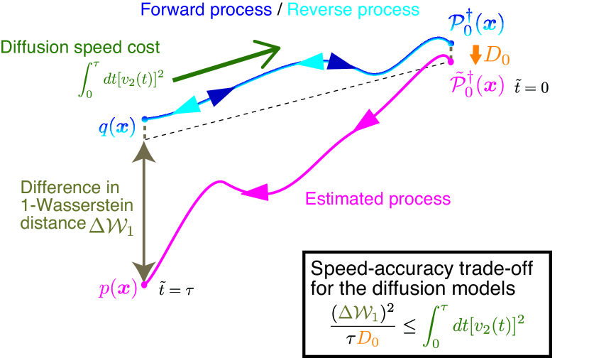
Figure 2: Illustration of the speed-accuracy trade-off for the diffusion models. We evaluate the difference between the initial conditions of the reverse process $\mathcal{P}^{\dagger}_{0}$ and the estimated process $\tilde{\mathcal{P}}^{\dagger}_{0}$ by the Person’s $\chi^{2}$-divergence $D_{0}$, and the estimation error of the generated data by the change of the $1$-Wasserstein distance $\Delta\mathcal{W}_{1}$. The speed-accuracy trade-off for the diffusion models implies that the diffusion speed cost $\int_{0}^{\tau}d{t}[v_{2}(t)]^{2}$ measured by the $2$-Wasserstein distance in the forward process affects the accuracy of the generated data given by the response function $(\Delta\mathcal{W}_{1})^{2}/D_{0}$.

According to the speed-accuracy trade-off for the diffusion models [Eq. (79)], we can consider minimizing the diffusion speed cost $\int_{0}^{\tau}d{t}[v_{2}(t)]^{2}$ to increase the accuracy of data generation, which is quantified by the smallness of the response function $(\Delta\mathcal{W}_{1})^{2}/D_{0}$. Therefore, minimizing the diffusion speed cost $\int_{0}^{\tau}d{t}[v_{2}(t)]^{2}$ can improve the performance of the diffusion model. When the initial state $\mathcal{P}_{0}$, the final state $\mathcal{P}_{\tau}$, and the time duration $\tau$ are fixed, the minimization problem can be discussed based on the geodesic in the $2$-Wasserstein metric space. We discuss this minimization problem of the diffusion speed cost in Sec. IV.3.

As an instantaneous expression of the speed-accuracy trade-off for the diffusion models, the following detailed inequality can be derived,

$$\frac{[\partial_{t}\mathcal{W}_{1}({\mathcal{P}}^{\dagger}_{\tau-t},\tilde{\mathcal{P}}_{\tau-t}^{\dagger})]^{2}}{{D}_{0}}\leq T_{t}\dot{S}_{t}^{\rm tot}.$$ (80)

When the external force is conservative, $T_{t}\dot{S}_{t}^{\rm tot}=[v_{2}(t)]^{2}$ holds and this inequality indicates that the speed in the space of the $2$-Wasserstein distance $v_{2}(t)$ is the upper bound on the change rate of the normalized estimation error $v_{\rm loss}(t):=|\partial_{t}\mathcal{W}_{1}({\mathcal{P}}^{\dagger}_{\tau-t},\tilde{\mathcal{P}}_{\tau-t}^{\dagger})|/\sqrt{{D}_{0}}$ as follows,

$$[v_{2}(t)]^{2}\geq[v_{\rm loss}(t)]^{2}.$$ (81)

This inequality is analogous to the thermodynamic uncertainty relation [Eq. (74)]. Using $v_{\rm loss}(t)$, we also obtain the hierarchy of inequalities corresponding to the speed-accracy trade-off for the diffusion model as follows,

$$\frac{(\Delta\mathcal{W}_{1})^{2}}{\tau D_{0}}\leq\int_{0}^{\tau}dt[v_{\rm loss}(t)]^{2}\leq\int_{0}^{\tau}dt[v_{2}(t)]^{2},$$ (82)

which is analogous to the thermodynamic speed limit.

IV.2 Proofs of the main result

We show here the derivation of the main result. We start with the derivation of Eq. (80). For the sake of simplicity, we introduce a notation for the probability density function of the estimated process $\tilde{\mathcal{P}}_{t}(\bm{x}):=\tilde{\mathcal{P}}^{\dagger}_{\tau-t}(\bm{x})$ according to the time direction of the forward process. Based on the Kantrovich-Rubinstein duality, the $1$-Wasserstein distance is given by

$$\mathcal{W}_{1}({\mathcal{P}}^{\dagger}_{\tau-t},\tilde{\mathcal{P}}_{\tau-t}^{\dagger})=\mathcal{W}_{1}(\mathcal{P}_{t},\tilde{\mathcal{P}}_{t})=\mathbb{E}_{\mathcal{P}_{t}}[\psi^{*}_{t}]-\mathbb{E}_{\tilde{\mathcal{P}}_{t}}[\psi^{*}_{t}],$$ (83)

where $\psi^{*}_{t}=\underset{\psi\in\mathrm{Lip}^{1}}{\operatorname{argmax}}\left(\mathbb{E}_{\mathcal{P}_{t}}[\psi]-\mathbb{E}_{\tilde{\mathcal{P}}_{t}}[\psi]\right)$ is the optimal solution of the maximization problem [Eq. (58)]. Since we assume that the velocity field of the forward process is accurately reconstructed ($\hat{\bm{\nu}}_{t}(\bm{x})=\bm{\nu}_{t}^{\mathcal{P}}(\bm{x})$), the continuity equations for the reverse process and the estimated process [Eqs. (3) and (4)] are given by $\partial_{t}\mathcal{P}_{t}(\bm{x})=-\nabla\cdot\left(\bm{\nu}_{t}^{\mathcal{P}}(\bm{x})\mathcal{P}_{t}(\bm{x})\right)$ and $\partial_{t}\tilde{\mathcal{P}}_{t}(\bm{x})=-\nabla\cdot\left(\bm{\nu}_{t}^{\mathcal{P}}(\bm{x})\tilde{\mathcal{P}}_{t}(\bm{x})\right)$. Therefore, the time evolution of the difference between two probability density functions $\delta\mathcal{P}_{t}(\bm{x}):=\mathcal{P}_{t}(\bm{x})-\tilde{\mathcal{P}}_{t}(\bm{x})$ is given by

$$\partial_{t}\delta\mathcal{P}_{t}(\bm{x})=-\nabla\cdot\left(\bm{\nu}_{t}^{\mathcal{P}}(\bm{x})\delta\mathcal{P}_{t}(\bm{x})\right).$$ (84)

Using Eq. (84), we obtain

$$\partial_{t}\left(\mathbb{E}_{\mathcal{P}_{t}}[\psi]-\mathbb{E}_{\tilde{\mathcal{P}}_{t}}[\psi]\right)= \int d\bm{x}\;\psi(\bm{x})\partial_{t}\delta\mathcal{P}_{t}(\bm{x})$$

$$= \int d\bm{x}\;\nabla\psi(\bm{x})\cdot\bm{\nu}_{t}^{\mathcal{P}}(\bm{x})\delta\mathcal{P}_{t}(\bm{x}),$$ (85)

for any time-independent $1$-Lipshitz function $\psi\in\mathrm{Lip}^{1}$, where we used the partial integration and we assumed that $\delta\mathcal{P}_{t}(\bm{x})$ disappears at infinity. From the Cauchy–Schwarz inequality and the $1$-Lipshitz continuity $\|\nabla\psi(\bm{x})\|\leq 1$, we obtain

$$\left(\partial_{t}\left(\mathbb{E}_{\mathcal{P}_{t}}[\psi]-\mathbb{E}_{\tilde{\mathcal{P}}_{t}}[\psi]\right)\right)^{2}$$

$$=\left(\int d\bm{x}\;\nabla\psi(\bm{x})\cdot\bm{\nu}_{t}^{\mathcal{P}}(\bm{x})\delta\mathcal{P}_{t}(\bm{x})\right)^{2}$$

$$\leq\left(\int d\bm{x}\;\|\bm{\nu}_{t}^{\mathcal{P}}(\bm{x})\|^{2}\mathcal{P}_{t}(\bm{x})\right)\left(\int d\bm{x}\;\|\nabla\psi(\bm{x})\|^{2}\frac{(\delta\mathcal{P}_{t}(\bm{x}))^{2}}{\mathcal{P}_{t}(\bm{x})}\right)$$

$$\leq\left(\int d\bm{x}\;\|\bm{\nu}_{t}^{\mathcal{P}}(\bm{x})\|^{2}\mathcal{P}_{t}(\bm{x})\right)\left(\int d\bm{x}\;\frac{(\delta\mathcal{P}_{t}(\bm{x}))^{2}}{\mathcal{P}_{t}(\bm{x})}\right)$$

$$=T_{t}\dot{S}^{\rm tot}_{t}D_{\tau-t},$$ (86)

where ${D}_{\tau-t}$ is the Pearson’s $\chi^{2}$-divergence at time $\tilde{t}=\tau-t$ defined as ${D}_{\tau-t}:=\int d\bm{x}[{\mathcal{P}}^{\dagger}_{\tau-t}(\bm{x})-\tilde{\mathcal{P}}_{\tau-t}^{\dagger}(\bm{x})]^{2}/\mathcal{P}^{\dagger}_{\tau-t}(\bm{x})$. We can show that the time derivative of $D_{\tau-t}$ is $\partial_{t}D_{\tau-t}=0$ (see Appendix E). Therefore, $D_{\tau-t}=D_{0}\;(=\rm{const.})$ holds, and we obtain the inequality

$$\left|\partial_{t}\left(\mathbb{E}_{\mathcal{P}_{t}}[\psi]-\mathbb{E}_{\tilde{\mathcal{P}}_{t}}[\psi]\right)\right|\leq\sqrt{T_{t}\dot{S}^{\rm tot}_{t}D_{0}},$$ (87)

for any $1$-Lipshitz function $\psi\in\mathrm{Lip}^{1}$. We now implicitly assume the existence of $\partial_{t}\mathcal{W}_{1}({\mathcal{P}}^{\dagger}_{\tau-t},\tilde{\mathcal{P}}_{\tau-t}^{\dagger})$, which can be justified by the smoothness of $\mathcal{W}_{1}({\mathcal{P}}^{\dagger}_{\tau-t},\tilde{\mathcal{P}}_{\tau-t}^{\dagger})$ as a function of $t$. In the case of $\partial_{t}\mathcal{W}_{1}({\mathcal{P}}^{\dagger}_{\tau-t},\tilde{\mathcal{P}}_{\tau-t}^{\dagger})\geq 0$, we obtain the lower bound on $\sqrt{T_{t}\dot{S}^{\rm tot}_{t}D_{0}}$ as follows,

$$0\leq \partial_{t}\mathcal{W}_{1}({\mathcal{P}}^{\dagger}_{\tau-t},\tilde{\mathcal{P}}_{\tau-t}^{\dagger})$$

$$= \lim_{\Delta t\to+0}\frac{\mathcal{W}_{1}(\mathcal{P}_{t},\tilde{\mathcal{P}}_{t})-\mathcal{W}_{1}(\mathcal{P}_{t-\Delta t},\tilde{\mathcal{P}}_{t-\Delta t})}{\Delta t}$$

$$\leq \lim_{\Delta t\to+0}\left[\frac{\mathbb{E}_{\mathcal{P}_{t}}[\psi^{*}_{t}]-\mathbb{E}_{\tilde{\mathcal{P}}_{t}}[\psi^{*}_{t}]-\mathbb{E}_{\mathcal{P}_{t-\Delta t}}[\psi^{*}_{t}]+\mathbb{E}_{\tilde{\mathcal{P}}_{t-\Delta t}}[\psi^{*}_{t}]}{\Delta t}\right]$$

$$= \left.\partial_{t}\left(\mathbb{E}_{\mathcal{P}_{t}}[\psi^{*}_{s}]-\mathbb{E}_{\tilde{\mathcal{P}}_{t}}[\psi^{*}_{s}]\right)\right|_{s=t}\leq\sqrt{T_{t}\dot{S}^{\rm tot}_{t}D_{0}},$$ (88)

where we used the fact that $\mathcal{W}_{1}(\mathcal{P}_{t-\Delta t},\tilde{\mathcal{P}}_{t-\Delta t})=\mathbb{E}_{\mathcal{P}_{t-\Delta t}}[\psi^{*}_{t-\Delta t}]-\mathbb{E}_{\tilde{\mathcal{P}}_{t-\Delta t}}[\psi^{*}_{t-\Delta t}]\geq\mathbb{E}_{\mathcal{P}_{t-\Delta t}}[\psi^{*}_{t}]-\mathbb{E}_{\tilde{\mathcal{P}}_{t-\Delta t}}[\psi^{*}_{t}]$ holds because of the definition of the $1$-Wasserstein distance, and we used the fact that Eq. (86) holds for any $t$-independent $1$-Lipshitz function $\psi^{*}_{s}\in\mathrm{Lip}^{1}$. In the case of $\partial_{t}\mathcal{W}_{1}({\mathcal{P}}^{\dagger}_{\tau-t},\tilde{\mathcal{P}}_{\tau-t}^{\dagger})\leq 0$, we obtain the lower bound on $\sqrt{T_{t}\dot{S}^{\rm tot}_{t}D_{0}}$ similarly as follows,

$$0\leq -\partial_{t}\mathcal{W}_{1}({\mathcal{P}}^{\dagger}_{\tau-t},\tilde{\mathcal{P}}_{\tau-t}^{\dagger})$$

$$= \lim_{\Delta t\to+0}\frac{\mathcal{W}_{1}(\mathcal{P}_{t},\tilde{\mathcal{P}}_{t})-\mathcal{W}_{1}(\mathcal{P}_{t+\Delta t},\tilde{\mathcal{P}}_{t+\Delta t})}{\Delta t}$$

$$\leq \left.-\partial_{t}\left(\mathbb{E}_{\mathcal{P}_{t}}[\psi^{*}_{s}]-\mathbb{E}_{\tilde{\mathcal{P}}_{t}}[\psi^{*}_{s}]\right)\right|_{s=t}\leq\sqrt{T_{t}\dot{S}^{\rm tot}_{t}D_{0}},$$ (89)

where we used the inequality $\mathcal{W}_{1}(\mathcal{P}_{t+\Delta t},\tilde{\mathcal{P}}_{t+\Delta t})=\mathbb{E}_{\mathcal{P}_{t+\Delta t}}[\psi^{*}_{t+\Delta t}]-\mathbb{E}_{\tilde{\mathcal{P}}_{t+\Delta t}}[\psi^{*}_{t+\Delta t}]\geq\mathbb{E}_{\mathcal{P}_{t+\Delta t}}[\psi^{*}_{t}]-\mathbb{E}_{\tilde{\mathcal{P}}_{t+\Delta t}}[\psi^{*}_{t}]$ and Eq. (86). By squaring both sides of the inequalities (88) and (89), the resulting inequalities are equivalent to Eq. (80). Thus, our main result Eq. (80) is proved regardless of the sign of $\partial_{t}\mathcal{W}_{1}({\mathcal{P}}^{\dagger}_{\tau-t},\tilde{\mathcal{P}}_{\tau-t}^{\dagger})$.

We next derive Eq. (77). By integrating Eq. (80) with respect to time and applying the Cauchy-Schwartz inequality, we obtain

$$\int_{0}^{\tau}dtT_{t}\dot{S}_{t}^{\rm tot} \geq\frac{1}{D_{0}}\int_{0}^{\tau}d{t}[\partial_{t}\mathcal{W}_{1}(\mathcal{P}_{t},\tilde{\mathcal{P}}_{t})]^{2}$$

$$\geq\frac{1}{\tau D_{0}}\left(\int_{0}^{\tau}\;d{t}\;\partial_{t}\mathcal{W}_{1}(\mathcal{P}_{t},\tilde{\mathcal{P}}_{t})\right)^{2}$$

$$=\frac{\left(\Delta\mathcal{W}_{1}\right)^{2}}{\tau D_{0}},$$ (90)

which is equivalent to Eq. (77). When the external force is conservative, Eq. (90) can be written as Eq. (82) because $T_{t}\dot{S}_{t}^{\rm tot}=[v_{2}(t)]^{2}$ and $v_{\rm loss}(t)=|\partial_{t}\mathcal{W}_{1}({\mathcal{P}}^{\dagger}_{\tau-t},\tilde{\mathcal{P}}_{\tau-t}^{\dagger})|/\sqrt{{D}_{0}}$.

IV.3 Optimality in the noise schedule

We discuss the diffusion speed cost $\int_{0}^{\tau}dt[v_{2}(t)]^{2}$, which is the upper bound on the response function in the speed-accuracy trade-off for the diffusion models [Eq. (79)]. Lowering this upper bound means making the response function $(\Delta\mathcal{W}_{1})^{2}/D_{0}$ small, and this lowering leads to robust data generation against perturbations of the initial distribution in the estimated process. Since the diffusion speed cost depends only on the dynamics of the forward process, it is possible to discuss an optimality of the noise schedules based on the diffusion speed cost. Similar to the discussion of the minimum entropy production [Eq. (68)], the lower bound of the diffusion speed cost is given by

$$\int_{0}^{\tau}dt[v_{2}(t)]^{2}\geq\frac{\mathcal{L}^{2}_{\tau}}{\tau}\geq\frac{(\mathcal{W}_{2}(\mathcal{P}_{0},\mathcal{P}_{\tau}))^{2}}{\tau}.$$ (91)

The equality condition is $v_{2}(t)=\mathcal{W}_{2}(\mathcal{P}_{0},\mathcal{P}_{\tau})/\tau$ that makes the time evolution of $\mathcal{P}_{t}$ be driven along the geodesic in the space of the $2$-Wasserstein distance. This time evolution can be discussed in terms of the optimal transport protocol discussed in Ref. [107]. At least from the perspective of the speed-accuracy trade-off for the diffusion models, an optimal noise schedule is introduced by considering the optimal transport which makes the time evolution of $\mathcal{P}_{t}$ driven along the geodesic in the space of the $2$-Wasserstein distance. We illustrate the example of an optimal noise schedule given by the optimal transport compared to other noise schedules such as the cosine schedule and the cond-OT schedule (see Fig.3).

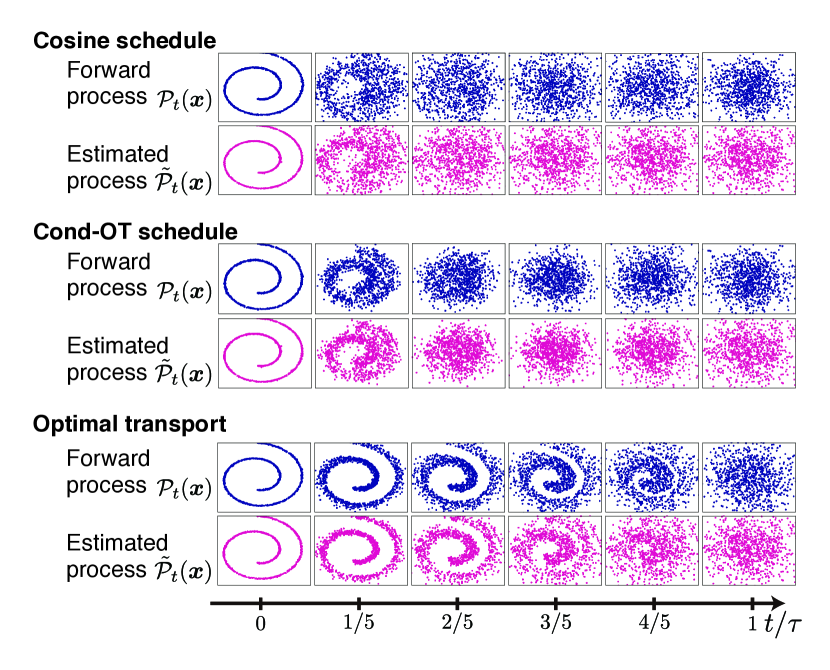
Figure 3: Examples of the forward process and the estimated process according to three noise schedules: the cosine schedule [Eq. (32)], the cond-OT schedule [Eq. (28)], and the optimal transport which gives the dynamics along the geodesic in the space of the 2-Wasserstein distance. These figures show the time evolution of samples from a $2$-dimensional Swiss roll dataset ($n_{\rm{d}}=2$) in the flow-based generative modeling. In all noise schedules, we used the same sample for the initial distribution of the estimated process $\tilde{\mathcal{P}}_{\tau}(\bm{x})$. Compared with the cosine schedule and the cond-OT schedule, the noise in the generated figure is relatively small when we consider the optimal transport. This result is consistent with the optimality based on the speed-accuracy trade-off for the diffusion models.

While optimal transport can lead to accurate data generation, it is computationally difficult to construct the diffusion process that achieves optimal transport in high-dimensional data. Therefore, the cond-OT schedule, which can be considered as an approximate optimal transport, is proposed. If the input distribution $q(\bm{x})$ is normalized such that $\mathbb{E}_{q}[\bm{x}]=\bm{0}$ and $\mathbb{E}_{q}[\|\bm{x}\|^{2}]=n_{\rm d}$, and the external force and the temperature are given by Eqs. (22) and (23), the diffusion speed cost is given asymptotically by the conditional kinetic energy $\mathcal{E}_{\rm c}$ [69] in the limit $N_{\rm D}/\sqrt{n_{\rm d}}\to 0$,

$$\int_{0}^{\tau}dt\left[v_{2}(t)\right]^{2}\simeq\tau n_{\rm d}\mathcal{E}_{\rm c},$$ (92)

where the dimension of the data $n_{\rm d}$ is sufficiently large against the number of data $N_{\rm D}$ [Theorem 4.2 in Ref. [69]]. Here, the conditional kinetic energy $\mathcal{E}_{\rm c}$ for the conditional Gaussian probabilities are given by $\mathcal{E}_{\rm c}=(1/\tau)\int_{0}^{\tau}dt[(\partial_{t}\sigma_{t})^{2}+(\partial_{t}m_{t})^{2}]$ [69]. Thus, if the data dimension is sufficiently larger than the number of data, the optimality based on the speed-accuracy trade-off for the diffusion model can be discussed by considering the minimization of this quantity $n_{\rm d}\int_{0}^{\tau}dt[(\partial_{t}\sigma_{t})^{2}+(\partial_{t}m_{t})^{2}]$ instead of the minimization of the diffusion speed cost $\int_{0}^{\tau}dt[v_{2}(t)]^{2}$.

We explain that minimizing $n_{\rm d}\int_{0}^{\tau}dt[(\partial_{t}\sigma_{t})^{2}+(\partial_{t}m_{t})^{2}]$ leads to the cond-OT schedule [Eq. (28)] and the cosine schedule [Eq. (32)]. When $\sigma_{t}$ and $m_{t}$ are unconstrained, we obtain an lower bound

$$n_{\rm d}\int_{0}^{\tau}dt[(\partial_{t}\sigma_{t})^{2}+(\partial_{t}m_{t})^{2}]$$

$$\geq n_{\rm d}\frac{(\sigma_{0}-\sigma_{\tau})^{2}+(m_{0}-m_{\tau})^{2}}{\tau},$$ (93)

from the Cauchy-Schwarz inequality. The equality conditions of this inequality are $\partial_{t}\sigma_{t}=(\sigma_{\tau}-\sigma_{0})/\tau$ and $\partial_{t}m_{t}=(m_{\tau}-m_{0})/\tau$, which can be regarded as the cond-OT schedule [Eq. (28)]. Under the constraint of the VP-diffusion, $\sigma_{t}^{2}+m_{t}^{2}=1$, we can introduce the angle $\theta_{t}$ which satisfies $(m_{t},\sigma_{t})=(\cos\theta_{t},\sin\theta_{t})$. From the Cauchy-Schwarz inequality, we also obtain another lower bound

$$n_{\rm d}\int_{0}^{\tau}dt[(\partial_{t}\sigma_{t})^{2}+(\partial_{t}m_{t})^{2}] =n_{\rm d}\int_{0}^{\tau}dt[(\partial_{t}\theta_{t})^{2}]$$

$$\geq n_{\rm d}\frac{(\theta_{0}-\theta_{\tau})^{2}}{\tau}.$$ (94)

The equality condition of this inequality is $\partial_{t}\theta_{t}=(\theta_{\tau}-\theta_{0})/\tau$, which can be regarded as the cosine schedule [Eq. (32)]. The cond-OT schedule or the cosine schedule are considered practical suboptimal protocols in terms of the speed-accuracy trade-off for the diffusion model when the dimension of the data is sufficiently larger than the number of data.

IV.4 Numerical experiments

Finally, we illustrate the validity of the speed-accuracy trade-off for the diffusion models by simple numerical experiments. We consider the $1$-dimensional flow-based generative modeling ($\bm{x}\in\mathbb{R}$). We now consider the situation where the velocity field of the forward process is accurately reconstructed and $q(\bm{x})$ is given by the Gaussian mixture distribution

$$q(\bm{x})=\frac{1}{2}\mathcal{N}(\bm{x}|m^{\rm a},\sigma^{2})+\frac{1}{2}\mathcal{N}(\bm{x}|m^{\rm b},\sigma^{2}).$$ (95)

Here, $\mathcal{N}(\bm{x}|m,\sigma^{2})$ is the $1$-dimensional Gaussian distribution with the mean $m$ and the variance $\sigma^{2}$. The velocity field $\bm{\nu}_{t}^{\mathcal{P}}(\bm{x})(\in\mathbb{R})$ can be calculated analytically as follows (see Appendix F for the detail of the numerical calculation),

$$\bm{\nu}_{t}^{\mathcal{P}}(\bm{x})=\frac{\partial_{t}\sigma_{t}}{\sigma_{t}}\bm{x}-\frac{m_{t}}{\mathcal{P}_{t}(\bm{x})}\left(\frac{\partial_{t}\sigma_{t}}{\sigma_{t}}-\frac{\partial_{t}m_{t}}{m_{t}}\right)\mathbb{E}_{\mathcal{P}^{c}_{t},q}[\bm{y}],$$ (96)

$$\mathbb{E}_{\mathcal{P}^{c}_{t},q}[\bm{y}]=\frac{1}{2}\frac{\sigma^{2}m_{t}\bm{x}+\sigma_{t}^{2}m^{\rm a}\bm{1}}{\sigma_{t}^{2}+\sigma^{2}m_{t}^{2}}\mathcal{N}^{\rm a}+\frac{1}{2}\frac{\sigma^{2}m_{t}\bm{x}+\sigma_{t}^{2}m^{\rm b}\bm{1}}{\sigma_{t}^{2}+\sigma^{2}m_{t}^{2}}\mathcal{N}^{\rm b},$$ (97)

where $\mathcal{N}^{\rm a}$ and $\mathcal{N}^{\rm b}$ are the Gaussian distributions defined as $\mathcal{N}^{\rm x}=\mathcal{N}\left(\bm{x}|m_{t}m^{\rm x},\sigma_{t}^{2}+\sigma^{2}m_{t}^{2}\right)\;({\rm x}={\rm a},{\rm b})$. We set the parameters $m^{\rm a}=-m^{\rm b}=\sqrt{0.35}$ and $\sigma=0.3$. We now consider the several perturbations of the initial condition in the estimated process $\tilde{\mathcal{P}}^{\dagger}_{0}(\bm{x})$ at $\tilde{t}=0$ (see also Appendix F for the detail). We numerically calculate the quantities in the speed-accuracy trade-off for the diffusion models [Eqs. (79) and (82)] and its differential form [Eq. (80)] in Fig. 4.

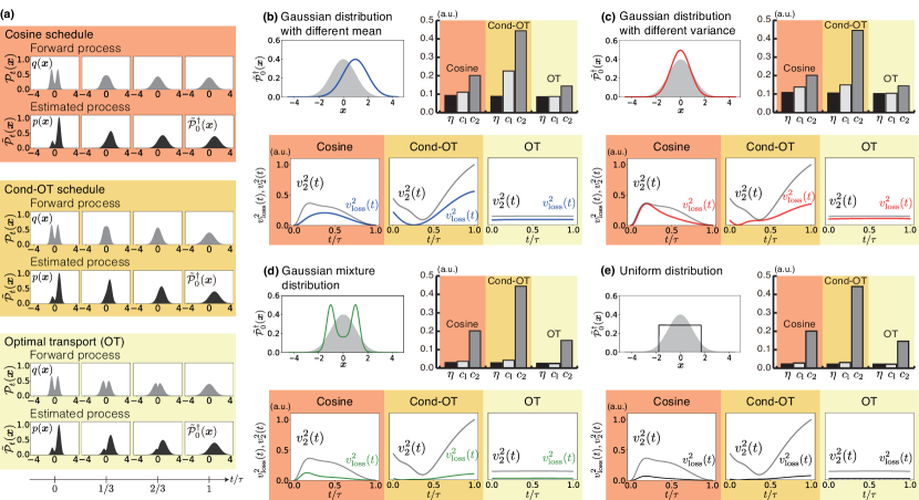
Figure 4: Numerical calculations of the speed-accuracy trade-off for the diffusion models [Eqs. (79), (80) and (82)]. (a) The time evolution of the probability density functions in the forward process and the estimated process with the cosine schedule, the cond-OT schedule and the optimal transport (OT). Here $t$ denotes time in the forward direction, and we show the probability density functions at $t=0$, $t=\tau/3$, $t=2\tau/3$ and $t=\tau$. The final state of the forward process is $\mathcal{P}_{\tau}(\bm{x})=\mathcal{N}(\bm{x}|0,1)$. We used a Gaussian distribution with different mean $\tilde{\mathcal{P}}_{0}^{\dagger}(\bm{x})=\mathcal{N}(\bm{x}|1,1)$ as the initial condition of the estimated process. (b-e) We show the situation where the initial condition of the estimated process $\tilde{\mathcal{P}}_{0}^{\dagger}(\bm{x})$ is (b) a Gaussian distribution with different mean, (c) a Gaussian distribution with different variance, (d) a Gaussian mixture distribution, (e) a uniform distribution. The plot at the top left of each section shows the comparison between $\tilde{\mathcal{P}}_{0}^{\dagger}(\bm{x})$ and $\mathcal{P}_{\tau}(\bm{x})=\mathcal{N}(\bm{x}|0,1)$, where $\mathcal{N}(\bm{x}|0,1)$ is shown in grey. In the top right-hand section, we show the bar graph which displays the quantities $\eta=(\Delta\mathcal{W}_{1})^{2}/(\tau D_{0})$, $c_{\rm l}=\int_{0}^{\tau}dt\;[v_{\rm loss}(t)]^{2}$, $c_{2}=\int_{0}^{\tau}dt\;[v_{2}(t)]^{2}$, and this figure shows the validity of the inequality $\eta\leq c_{1}\leq c_{2}$ [Eq. (82)]. In the bottom row we show the time evolution of $[v_{2}(t)]^{2}$ and $[v_{\rm loss}(t)]^{2}$, and this figure shows the validity of the inequality $[v_{2}(t)]^{2}\geq[v_{\rm loss}(t)]^{2}$ [Eq. (80)]. Since $[v_{2}(t)]^{2}$ and $c_{2}$ depend only on the forward process, these values are consistent within different initial conditions in (b)-(e). See also Table 2 in Appendix F for more detailed explanations, including the probability density function $\tilde{\mathcal{P}}_{0}^{\dagger}(\bm{x})$ used in (b)-(e).

We discuss the interpretations of the numerical results in Fig. 4. In Fig. 4(a), we show the time evolution of the probability density functions in the forward process $\mathcal{P}_{t}(\bm{x})$ and the time evolution of the probability density functions in the estimated process $\tilde{\mathcal{P}}_{t}(\bm{x})$ with three noise schedules: the cosine schedule, the cond-OT schedule and the optimal transport. We remark that the cosine and cond-OT schedules are not considered the optimal transport because we now consider the situation where $N_{\rm D}/\sqrt{n_{\rm d}}$ is not sufficiently small. The initial condition in the estimated process $\mathcal{P}_{0}^{\dagger}(\bm{x})$ is fixed to the Gaussian distribution $\mathcal{N}(\bm{x}|1,1)$ while the final state in the forward process is given by the Gaussian distribution $\mathcal{N}(\bm{x}|0,1)$. In Appendix F, we also show the cases of other initial conditions $\mathcal{P}_{0}^{\dagger}(\bm{x})$ (see also Fig. 5). In Fig. 4(a), the probability density functions in the forward process with the cosine schedule and the cond-OT schedule are significantly changed between time $t=0$ and $t=(1/3)\tau$ compared to the optimal transport. Thus, the data structure corresponding to the two peaks of the probability density function is not well recovered in the estimated process with the cosine and cond-OT schedules between $t=(1/3)\tau$ and $t=\tau$ while the two peaks can be seen between $t=(1/3)\tau$ and $t=(2/3)\tau$ in the estimated process with the optimal transport.

Next, we numerically confirm the speed-accuracy trade-off for the diffusion models [Eqs. (79) and (82)] and the detailed inequality [Eq. (80)] hold under the various conditions of $\mathcal{P}_{0}^{\dagger}(\bm{x})$ in Fig. 4(b)-(e): (b) a Gaussian distribution with different mean, (c) a Gaussian distribution with different variance, (d) a Gaussian mixture distribution and (e) a uniform distribution. Here, we used the notation $\eta\leq c_{1}\leq c_{2}$ for Eq. (82), where $\eta=(\Delta\mathcal{W}_{1})^{2}/D_{0}$, $c_{1}=\int_{0}^{\tau}dt[v_{\rm loss}(t)]^{2}$ and $c_{2}=\int_{0}^{\tau}dt[v_{2}(t)]^{2}$. We confirm that the speed-accuracy trade-off for the diffusion models are valid under all conditions. We also observe that the bounds in Eq. (80) are tighter in the case of optimal transport (OT) than the bounds in the cases of cosine and cond-OT schedules. There is a tendency for the bound in the detailed inequality [Eq. (80)] to become loose during the time evolution for the cosine schedule, and the bound in the detailed inequality [Eq. (80)] to become loose at the beginning and at the end of the time evolution for the cond-OT schedule. The upper bounds of the response function $\eta$, namely $c_{1}$ and $c_{2}$, are tighter for the optimal transport compared to the cosine and cond-OT schedules. The value of the response function $\eta$ for the optimal transport is also the smallest for any schedule (see Tab. 1), which supports our conclusion that the optimal transport provides the most accurate data generation.

Initial conditions	Noise schedules	Values of $\eta$
Gaussian distribution with different mean	Cosine Cond-OT OT	$9.1884\times 10^{-2}$ $8.7810\times 10^{-2}$ $8.5375\times 10^{-2}$
Gaussian distribution with different variance	Cosine Cond-OT OT	$1.0780\times 10^{-1}$ $1.0477\times 10^{-1}$ $1.0224\times 10^{-1}$
Gaussian mixture distribution	Cosine Cond-OT OT	$2.7649\times 10^{-2}$ $2.6747\times 10^{-2}$ $2.6119\times 10^{-2}$
Uniform distribution	Cosine Cond-OT OT	$2.1420\times 10^{-2}$ $2.0680\times 10^{-2}$ $2.0333\times 10^{-2}$

Table 1: The values of the response function $\eta=(\Delta\mathcal{W}_{1})^{2}/(\tau D_{0})$ in the numerical calculations [Fig. 4]. Since we computed $3\times 10^{9}$ samples, we display the value with five significant digits.

Interestingly, although the values of the upper bounds $c_{1}$ and $c_{2}$ for the optimal transport are so small compared to the cosine and cond-OT schedules, the value of the response function $\eta$ for the optimal transport is not so small compared to the cosine and cond-OT schedules. In fact, the probability density functions corresponding to the generated data $p(\bm{x})$ in Fig. 4(a) are not significantly different under different conditions. The reason for this fact may be that we are only considering a simple data structure of $1$-dimensional Gaussian mixtures, so larger differences in $\eta$ between different noise schedules may occur when the data structure is more complex. Reducing the time duration $\tau$ and rapidly changing the time evolution in the forward process may also cause large $\eta$ differences between different noise schedules.

Our discussion based on the speed-accuracy trade-off for the diffusion models may not be sufficient to explain why the cosine and cond-OT schedules work well even when $N/\sqrt{n_{\rm d}}$ is not sufficiently small. Since the value of $\eta$ is indeed approximately equal to the value of $c_{1}$ for the optimal transport, the value of $\eta$ itself can be considered to be determined by the speed-accuracy trade-off for the diffusion models. To understand why the response function $\eta$ for the optimal transport is not so small compared to the cosine and cond-OT schedules, it may be necessary to consider not only the upper bound on $\eta$ derived in this paper, but also the lower bound on $\eta$.

V Discussions

In this paper, we summarize the relationship between diffusion models and nonequilibrium thermodynamics, and derive the speed-accuracy trade-off for diffusion models based on techniques from stochastic thermodynamics and optimal transport theory. The speed-accuracy trade-off for diffusion models explains that the robustness of data generation to perturbations is generally limited by the thermodynamic dissipation in the forward diffusion process. The speed-accuracy trade-off for diffusion models also quantitatively explains the validity of using the cosine and cond-OT schedules as the noise schedules in the diffusion model and the importance of using optimal transport in the forward diffusion process.

In this paper, we derive the speed-accuracy trade-off for the diffusion models as analogs of the thermodynamic trade-off relations such as the thermodynamic uncertainty relation [112, 114, 108] and the thermodynamic speed limit [30, 29]. Unlike the conventional thermodynamic trade-off relation, which considers thermodynamic limits on the speed of the observable in a stochastic process, the speed-accuracy trade-off for the diffusion model is conceptually different because it gives a limit on how the difference between two different processes, the forward process and the estimated process, changes. This result is due to the error-free estimation of the velocity field in the forward process and its use in the estimated process. If the velocity field estimation is incomplete, then corrections to the speed-accuracy trade-off for the diffusion model would have to be made due to the incompleteness. Even in the case of incomplete estimation, it is an open question whether using the dynamics of optimal transport as the forward process is best in terms of robustness of data generation.

We believe that in this paper we have demonstrated only one aspect of the usefulness of the analogy between diffusion models and stochastic thermodynamics. We believe that the conventional thermodynamic uncertainty relations [114, 112, 21, 24, 108] are also useful because we can consider the speed of any observable in the forward process, for example, the speed of data structure breakage in the diffusion process. It is also noteworthy that the short-time thermodynamic uncertainty relation is used to estimate the time-varying velocity field [21, 23], which is important in the flow-based generative modeling, and it is worth considering whether there are any aspects in which such a thermodynamic-based method is superior to conventional flow matching methods.

It is also interesting to reconsider the path probability based method as discussed in the original paper on the diffusion model from a thermodynamic point of view. This is because the method discussed in the original paper can handle not only the simple diffusion processes described by the Langevin and Fokker-Planck equations, but also the diffusion process on the graph described by the Markov jump processes, which may provide a scalable method than the current one. In such a case, the thermodynamic trade-off relations and optimal transport for the Markov jump process [115, 116, 117, 118] may be useful to consider the optimality of the diffusion model. In such a case, analogies to an information geometric structure of the Kullback-Leibler divergence in stochastic thermodynamics [103, 118, 32] may also be important, since the loss function is introduced by the Kullback-Leibler divergence and its minimization is mathematically well discussed as the projection theorem in information geometry [83]. In fact, there are several stochastic methods based on the Schrödinger bridge in the diffusion model [119, 120, 50, 71], which is given by the minimization of the Kullback-Leibler divergence. We may be able to obtain some trade-off relations for such a system by considering an analogy to stochastic thermodynamics based on path probability.

We explain how the speed-accuracy trade-off for the diffusion models can be positioned within the existing evaluation of diffusion models. The speed-accuracy trade-off for the diffusion models gives the upper bound on the estimation error using the $1$-Wasserstein distance. Several studies are known to provide bounds on the estimation error, such as the Kullback-Leibler divergence [121], the total variation distance [122, 123], and the Wasserstein distance [65, 66, 67]. These studies mainly focus on evaluating the effect of incomplete estimation on the generative data. Thus, these studies are fundamentally different from our approach, which assumes an accurate estimation of the velocity field and evaluates the effect of the perturbation on the initial state of the estimated process and the noise schedules. In other words, the speed-accuracy trade-off for the diffusion models can be thought of as a bound that evaluates structure-based properties of the diffusion models that are independent of the estimation method.

While there have been many numerical attempts to investigate the effect of noise schedules on the quality of data generation [43, 124, 63, 73, 97], there are almost no theoretical studies that investigate their effect on the estimation error based on the universal upper bound. The speed-accuracy trade-off for the diffusion models derived in this study may provide insight into how to determine this noise schedule for accurate data generation. In fact, we have shown that the existing methods, such as the cosine and cond-OT schedules, are suboptimal from the perspective of the speed-accuracy trade-off for the diffusion models. Thus, these methods have room for improvement, and the room for improvement can be discussed quantitatively based on the tightness of the inequalities.

Our conclusion for the noise schedule is also justified in light of recent developments in the diffusion model. In our conclusion, the optimal forward process for the data generation should be given by the geodesic in the space of the $2$-Wasserstein distance. In recent years, several methods have been proposed to realize the dynamics along the geodesic approximately in the flow-based generative modeling and the probability flow ODE [72, 125, 70, 69, 68], which is becoming the mainstream methods.

Appendix A Derivation of the relations between the two gradients of the objective functions

We show $\nabla_{\theta}L_{\rm SM}^{\rm c}(\theta)=\nabla_{\theta}L_{\rm SM}(\theta)$ for solving the optimization problem by score matching, and that $\nabla_{\theta}L_{\rm FM}^{\rm c}(\theta)=\nabla_{\theta}L_{\rm FM}(\theta)$ is satisfied for solving the optimization problem by flow matching.

A.0.1 Score matching

We show that two objective functions

$$L_{\rm{SM}}(\theta)=\mathbb{E}_{\mathcal{P}_{t},\mathcal{U}}\left[\|\bm{s}^{\theta}_{t}(\bm{x})-\nabla\ln\mathcal{P}_{t}(\bm{x})\|^{2}\right],$$ (98)

and

$$L^{\rm c}_{\rm{SM}}(\theta)=\mathbb{E}_{\mathcal{P}^{\rm c}_{t},q,\mathcal{U}}\left[\|\bm{s}^{\theta}_{t}(\bm{x})-\nabla\ln\mathcal{P}^{c}_{t}(\bm{x}|\bm{y})\|^{2}\right],$$ (99)

give the same gradient for the parameter $\theta$. The gradient $\nabla_{\theta}L^{\rm c}_{\rm{SM}}(\theta)$ can be calculated as follows,

$$\nabla_{\theta}L^{\rm c}_{\rm{SM}}(\theta)= \frac{2}{\tau}\int_{0}^{\tau}dt\int d\bm{x}\int d\bm{y}\mathcal{P}^{\rm c}_{t}(\bm{x}|\bm{y})q(\bm{y})[\nabla_{\theta}\bm{s}^{\theta}_{t}(\bm{x})]\cdot\left(\bm{s}^{\theta}_{t}(\bm{x})-\frac{\nabla\mathcal{P}^{\rm c}_{t}(\bm{x}|\bm{y})}{\mathcal{P}^{\rm c}_{t}(\bm{x}|\bm{y})}\right)$$

$$= \frac{2}{\tau}\int_{0}^{\tau}dt\int d\bm{x}\mathcal{P}_{t}(\bm{x})[\nabla_{\theta}\bm{s}^{\theta}_{t}(\bm{x})]\cdot\left(\bm{s}^{\theta}_{t}(\bm{x})-\frac{\nabla\mathcal{P}_{t}(\bm{x})}{\mathcal{P}_{t}(\bm{x})}\right)$$

$$= \nabla_{\theta}L_{\rm{SM}}(\theta),$$ (100)

which means that $\nabla_{\theta}L^{\rm c}_{\rm{SM}}(\theta)$ coincides with $\nabla_{\theta}L_{\rm{SM}}(\theta)$. Here, we used $\int d\bm{y}\mathcal{P}^{\rm c}_{t}(\bm{x}|\bm{y})q(\bm{y})=\mathcal{P}_{t}(\bm{x})$ and $q(\bm{y})\nabla\mathcal{P}^{\rm c}_{t}(\bm{x}|\bm{y})=\nabla[\mathcal{P}^{\rm c}_{t}(\bm{x}|\bm{y})q(\bm{y})]$.

A.0.2 Flow matching

Similarly, in flow matching, we show that two objective functions

$$L_{\rm{FM}}(\theta)=\mathbb{E}_{\mathcal{P}_{t},\mathcal{U}}\left[\|\bm{u}_{t}^{\theta}(\bm{x})-\bm{\nu}^{\mathcal{P}}_{t}(\bm{x})\|^{2}\right],$$ (101)

and

$$L^{c}_{\rm{FM}}(\theta)=\mathbb{E}_{\mathcal{P}_{t},q,\mathcal{U}}\left[\|\bm{u}_{t}^{\theta}(\bm{x})-\bm{\nu}^{\mathcal{P}^{c}}_{t}(\bm{x}|\bm{y})\|^{2}\right],$$ (102)

gives the same gradient for the parameter $\theta$. The gradient $\nabla_{\theta}L^{\rm c}_{\rm{FM}}(\theta)$ can be calculated as follows,

$$\nabla_{\theta}L^{\rm c}_{\rm{FM}}(\theta)= \frac{2}{\tau}\int dt\int d\bm{y}\int d\bm{x}\mathcal{P}^{\rm c}_{t}(\bm{x}|\bm{y})q(\bm{y})[\nabla_{\theta}\bm{u}_{t}^{\theta}(\bm{x})]\cdot(\bm{u}_{t}^{\theta}(\bm{x})-\bm{\nu}^{\mathcal{P}^{\rm c}}_{t}(\bm{x}|\bm{y}))$$

$$= \frac{2}{\tau}\int dt\int d\bm{x}\mathcal{P}_{t}(\bm{x})[\nabla_{\theta}\bm{u}_{t}^{\theta}(\bm{x})]\cdot(\bm{u}_{t}^{\theta}(\bm{x})-\bm{\nu}^{\mathcal{P}}_{t}(\bm{x}))$$

$$= \nabla_{\theta}L_{\rm{FM}}(\theta),$$ (103)

which means that $\nabla_{\theta}L^{\rm c}_{\rm{FM}}(\theta)$ coincides with $\nabla_{\theta}L_{\rm{FM}}(\theta)$. Here, we used $\int d\bm{y}\mathcal{P}^{\rm c}_{t}(\bm{x}|\bm{y})q(\bm{y})=\mathcal{P}_{t}(\bm{x})$ and

$$\bm{\nu}_{t}^{\mathcal{P}}(\bm{x})\mathcal{P}_{t}(\bm{x})=\int d\bm{y}\bm{\nu}_{t}^{\mathcal{P}^{c}}(\bm{x}|\bm{y})\mathcal{P}_{t}^{c}(\bm{x}|\bm{y})q(\bm{y}).$$ (104)

Appendix B Parameters of the conditional probability density function

Here, we explain the specific expressions for the parameters $\bm{\mu}_{t}(\bm{y})$ and $\mathsf{\Sigma}_{t}$ of the conditional probability density function $\mathcal{P}^{\rm c}_{t}(\bm{x}|\bm{y})=\mathcal{N}(\bm{x}|\bm{\mu}_{t}(\bm{y}),\mathsf{\Sigma}_{t})$.The Fokker–Planck equation for the conditional probability density function $\mathcal{P}^{\rm c}_{t}(\bm{x}|\bm{y})$ is given as follows,

$$\partial_{t}\mathcal{P}^{\rm c}_{t}(\bm{x}|\bm{y}) =-\nabla\cdot\left(\bm{\nu}^{\mathcal{P}^{\rm c}}_{t}(\bm{x}|\bm{y})\mathcal{P}^{\rm c}_{t}(\bm{x}|\bm{y})\right),$$ (105)

$$\bm{\nu}_{t}^{\mathcal{P}^{\rm c}}(\bm{x}|\bm{y}) \coloneqq\mathsf{A}_{t}\bm{x}+\bm{b}_{t}-T_{t}\nabla\ln\mathcal{P}^{\rm c}_{t}(\bm{x}|\bm{y})=(\mathsf{A}_{t}+T_{t}\mathsf{\Sigma}_{t}^{-1})(\bm{x}-\bm{\mu}_{t}(\bm{y}))+\mathsf{A}_{t}\bm{\mu}_{t}(\bm{y})+\bm{b}_{t}.$$ (106)

Thus, the time evolution of the parameter $\bm{\mu}_{t}(\bm{y})$ can be calculated as follows,

$$\partial_{t}\bm{\mu}_{t}(\bm{y}) =\partial_{t}\int d\bm{x}\bm{x}\mathcal{P}^{\rm{c}}_{t}(\bm{x}|\bm{y})$$

$$=\int d\bm{x}\bm{x}\left(-\nabla\cdot\left(\bm{\nu}^{\mathcal{P}^{\rm c}}_{t}(\bm{x}|\bm{y})\mathcal{P}^{\rm c}_{t}(\bm{x}|\bm{y})\right)\right)$$

$$=\int d\bm{x}\bm{\nu}^{\mathcal{P}^{\rm c}}_{t}(\bm{x}|\bm{y})\mathcal{P}^{\rm c}_{t}(\bm{x}|\bm{y})$$

$$=\int d\bm{x}[A_{t}\bm{x}+\bm{b}_{t}]\mathcal{P}^{\rm c}_{t}(\bm{x}|\bm{y})-\int d\bm{x}T_{t}\nabla\mathcal{P}^{\rm c}_{t}(\bm{x}|\bm{y})$$

$$=\mathsf{A}_{t}\bm{\mu}_{t}(\bm{y})+\bm{b}_{t},$$ (107)

where we assumed that the contribution vanishes at infinity in the partial integration, and we used $\bm{\mu}_{t}(\bm{y})=\int d\bm{x}\bm{x}\mathcal{P}^{\rm{c}}_{t}(\bm{x}|\bm{y})$ and $\int d\bm{x}\nabla\mathcal{P}^{\rm c}_{t}(\bm{x}|\bm{y})=0$. The time evolution of the parameter $\mathsf{\Sigma}_{t}$ is also calculated as follows,

$$\partial_{t}\mathsf{\Sigma}_{t} =\partial_{t}\int d\bm{x}(\bm{x}-\bm{\mu}_{t}(\bm{y}))(\bm{x}-\bm{\mu}_{t}(\bm{y}))^{\top}\mathcal{P}^{\rm{c}}_{t}(\bm{x}|\bm{y})$$

$$=\int d\bm{x}(\bm{x}-\bm{\mu}_{t}(\bm{y}))(\bm{x}-\bm{\mu}_{t}(\bm{y}))^{\top}\left(-\nabla\cdot\left(\bm{\nu}^{\mathcal{P}^{\rm c}}_{t}(\bm{x}|\bm{y})\mathcal{P}^{\rm c}_{t}(\bm{x}|\bm{y})\right)\right)$$

$$=\int d\bm{x}(\mathsf{A}_{t}+T_{t}\mathsf{\Sigma}_{t}^{-1})(\bm{x}-\bm{\mu}_{t}(\bm{y}))(\bm{x}-\bm{\mu}_{t}(\bm{y}))^{\top}\mathcal{P}^{\rm c}_{t}(\bm{x}|\bm{y})+\int d\bm{x}(\bm{x}-\bm{\mu}_{t}(\bm{y}))\left[(\mathsf{A}_{t}+T_{t}\mathsf{\Sigma}_{t}^{-1})(\bm{x}-\bm{\mu}_{t}(\bm{y}))\right]^{\top}\mathcal{P}^{\rm c}_{t}(\bm{x}|\bm{y})$$

$$=\mathsf{A}_{t}\mathsf{\Sigma}_{t}+\mathsf{\Sigma}_{t}\mathsf{A}_{t}^{\top}+2T_{t}\mathsf{I},$$ (108)

where $\top$ stands for the transpose, and we used $\mathsf{\Sigma}_{t}=\int d\bm{x}(\bm{x}-\bm{\mu}_{t}(\bm{y}))(\bm{x}-\bm{\mu}_{t}(\bm{y}))^{\top}\mathcal{P}^{\rm{c}}_{t}(\bm{x}|\bm{y})$, $\int d\bm{x}(\bm{x}-\bm{\mu}_{t}(\bm{y}))\mathcal{P}^{\rm{c}}_{t}(\bm{x}|\bm{y})=\bm{0}$ and $(\mathsf{\Sigma}_{t}^{-1})^{\top}=\mathsf{\Sigma}_{t}^{-1}$.

Now, we consider a situation where $\mathsf{A}_{t}$, $\bm{b}_{t}$ and $T_{t}$ are expressed as $\mathsf{A}_{t}=(\partial_{t}\ln m_{t})\mathsf{I}$, $\bm{b}_{t}=\bm{0}$, $T_{t}=\partial_{t}(\sigma_{t}^{2}/2)-\sigma_{t}^{2}\partial_{t}\ln m_{t}$ with non-negative parameters $\sigma_{t}(\geq 0)$, $m_{t}(\geq 0)$, and the initial conditions of the parameters are given by $m_{t=0}=1$ and $\sigma_{t=0}=0$. In this situation, Eqs. (107) and (108) are given as follows,

$$\partial_{t}\bm{\mu}_{t}(\bm{y}) =(\partial_{t}\ln m_{t})\bm{\mu}_{t}(\bm{y}),$$ (109)

$$\partial_{t}\mathsf{\Sigma}_{t}(\bm{y}) =(2\partial_{t}\ln m_{t})\mathsf{\Sigma}_{t}(\bm{y})+(\partial_{t}(\sigma_{t}^{2})-2\sigma_{t}^{2}\partial_{t}\ln m_{t})\mathsf{I}.$$ (110)

Therefore, the $k$-th element of the vector $[\bm{\mu}_{t}(\bm{y})]_{k}$ and, the $(k,l)$ element of the matrix $[\mathsf{\Sigma}_{t}(\bm{y})]_{kl}$ satisfies the following equations,

$$\partial_{t}[\bm{\mu}_{t}(\bm{y})]_{k} =(\partial_{t}\ln m_{t})[\bm{\mu}_{t}(\bm{y})]_{k},$$ (111)

$$\partial_{t}([\mathsf{\Sigma}_{t}(\bm{y})]_{kl}-\sigma_{t}^{2}\delta_{kl}) =(2\partial_{t}\ln m_{t})([\mathsf{\Sigma}_{t}(\bm{y})]_{kl}-\sigma_{t}^{2}\delta_{kl}),$$ (112)

where $\delta_{kl}=[\mathsf{I}]_{kl}$ is the Kronecker delta. Because $\bm{\mu}_{t=0}(\bm{y})=\bm{y}$ and $\mathsf{\Sigma}_{t=0}=\mathsf{O}$, performing a time integral from $t=0$ to $t$ yields

$$[\bm{\mu}_{t}(\bm{y})]_{k} =m_{t}[\bm{y}]_{k},$$ (113)

$$[\mathsf{\Sigma}_{t}(\bm{y})]_{kl}-\sigma_{t}^{2}\delta_{kl} =0,$$ (114)

and thus the following specific expressions are obtained,

$$\bm{\mu}_{t}(\bm{y})=m_{t}\bm{y},\>\>\mathsf{\Sigma}_{t}=\mathsf{\sigma}_{t}^{2}\mathsf{I}.$$ (115)

Appendix C Coordinate transformation in the DDIM

We show the detailed calculation of the coordinate transformation in the DDIM. The Fokker–Planck equation [Eq. (1)] with Eq. (23) is given as follows,

$$\partial_{t}\mathcal{P}_{t}(\bm{x})=-\nabla\cdot\left[\left[(\partial_{t}\ln m_{t})\bm{x}-T_{t}\nabla\ln\mathcal{P}_{t}(\bm{x})\right]\mathcal{P}_{t}(\bm{x})\right].$$ (116)

From the coordinate transform

$$\bar{\bm{x}}=\frac{\bm{x}}{m_{t}},$$ (117)

we obtain $\mathcal{P}_{t}(\bm{x})=\bar{\mathcal{P}}_{t}(\bar{\bm{x}})(|d\bar{\bm{x}}/d\bm{x}|)=\bar{\mathcal{P}}_{t}(\bar{\bm{x}})(m_{t})^{-{n_{\rm d}}}$. By substituting this into Eq. (116), the left-hand side is calculated as

$$\partial_{t}\mathcal{P}_{t}(\bm{x})=(m_{t})^{-{n_{\rm d}}}\partial_{t}\bar{\mathcal{P}}_{t}(\bar{\bm{x}})-{n_{\rm d}}(\partial_{t}\ln m_{t})(m_{t})^{-{n_{\rm d}}}\bar{\mathcal{P}}_{t}(\bar{\bm{x}})-(\partial_{t}\ln m_{t})(m_{t})^{-(n_{\rm d}+1)}\bm{x}\cdot\nabla_{\bar{\bm{x}}}\bar{\mathcal{P}}_{t}(\bar{\bm{x}}),$$ (118)

where we defined $\nabla_{\bar{\bm{x}}}$ as $\nabla_{\bar{\bm{x}}}=m_{t}\nabla$. The right hand side of Eq. (116) is calculated as

$$-\nabla\cdot\left[\left[(\partial_{t}\ln m_{t})\bm{x}-T_{t}\nabla\ln\mathcal{P}_{t}(\bm{x})\right]\mathcal{P}_{t}(\bm{x})\right]$$

$$= -{n_{\rm d}}(\partial_{t}\ln m_{t})(m_{t})^{-{n_{\rm d}}}\bar{\mathcal{P}}_{t}(\bar{\bm{x}})-(\partial_{t}\ln m_{t})(m_{t})^{-(n_{\rm d}+1)}\bm{x}\cdot\nabla_{\bar{\bm{x}}}\bar{\mathcal{P}}_{t}(\bar{\bm{x}})+\nabla_{\bar{\bm{x}}}\cdot\left[\left[T_{t}\nabla_{\bar{\bm{x}}}\ln\bar{\mathcal{P}}_{t}(\bar{\bm{x}})\right]\bar{\mathcal{P}}_{t}(\bar{\bm{x}})(m_{t})^{-(n_{\rm d}+2)}\right].$$ (119)

From Eqs. (118) and (119), we obtain

$$\partial_{t}\bar{\mathcal{P}}_{t}(\bar{\bm{x}})=-\nabla_{\bar{\bm{x}}}\cdot\left[\left[-\frac{T_{t}}{(m_{t})^{2}}\nabla_{\bar{\bm{x}}}\ln\bar{\mathcal{P}}_{t}(\bar{\bm{x}})\right]\bar{\mathcal{P}}_{t}(\bar{\bm{x}})\right].$$ (120)

By substituting $T_{t}=-\partial_{t}\ln m_{t}$,

$$\partial_{t}\bar{\mathcal{P}}_{t}(\bar{\bm{x}})=-\nabla_{\bar{\bm{x}}}\cdot\left[\left[\frac{\partial_{t}\ln m_{t}}{(m_{t})^{2}}\nabla_{\bar{\bm{x}}}\ln\bar{\mathcal{P}}_{t}(\bar{\bm{x}})\right]\bar{\mathcal{P}}_{t}(\bar{\bm{x}})\right],$$ (121)

is derived.

Appendix D The relations between the Kullback–Leibler divergence and the entropy production

First, we prove that the Kullback–Leibler divergence

$$D_{\rm KL}(\mathbb{P}_{\rm F}\|\mathbb{P}_{\rm B}) =\sum_{N=0}^{N_{\tau}-1}\int d\Gamma\mathbb{P}_{\rm F}(\Gamma)\ln\frac{\mathcal{T}_{N\Delta t}(\bm{x}_{(N+1)\Delta t}|\bm{x}_{N\Delta t})}{\mathcal{T}^{\dagger}_{N\Delta t}(\bm{x}_{(N+1)\Delta t}|\bm{x}_{N\Delta t})},$$ (122)

coincides with the entropy production

$$S^{\rm tot}_{\tau}=\int_{0}^{\tau}dt\left[\frac{1}{T_{t}}\int d\bm{x}\|\bm{\nu}^{\mathcal{P}}_{t}(\bm{x})\|^{2}\mathcal{P}_{t}(\bm{x})\right],$$ (123)

in the limit $\Delta t\to 0$ with fixed $\tau$. By calculating $\ln[\mathcal{T}_{N\Delta t}(\bm{x}_{(N+1)\Delta t}|\bm{x}_{N\Delta t})/\mathcal{T}^{\dagger}_{N\Delta t}(\bm{x}_{(N+1)\Delta t}|\bm{x}_{N\Delta t})]$, we obtain

$$\ln\frac{\mathcal{T}_{N\Delta t}(\bm{x}_{(N+1)\Delta t}|\bm{x}_{N\Delta t})}{\mathcal{T}^{\dagger}_{N\Delta t}(\bm{x}_{(N+1)\Delta t}|\bm{x}_{N\Delta t})}$$

$$= \frac{\left\|\bm{x}_{(N+1)\Delta t}-\bm{x}_{N\Delta t}-\bm{f}_{N\Delta t}(\bm{x}_{N\Delta t})\Delta t+2\bm{\nu}_{N\Delta t}^{\mathcal{P}}(\bm{x}_{N\Delta t})\Delta t\right\|^{2}}{4T_{N\Delta t}\Delta t}-\frac{\left\|\bm{x}_{(N+1)\Delta t}-\bm{x}_{N\Delta t}-\bm{f}_{N\Delta t}(\bm{x}_{N\Delta t})\Delta t\right\|^{2}}{4T_{N\Delta t}\Delta t}$$

$$= \frac{\left\|\bm{\nu}_{N\Delta t}^{\mathcal{P}}(\bm{x}_{N\Delta t})\right\|^{2}}{T_{N\Delta t}}\Delta t+\frac{(\bm{x}_{(N+1)\Delta t}-\bm{x}_{N\Delta t}-\bm{f}_{N\Delta t}(\bm{x}_{N\Delta t})\Delta t)\cdot\bm{\nu}_{N\Delta t}^{\mathcal{P}}(\bm{x}_{N\Delta t})}{T_{N\Delta t}}.$$ (124)

By using $\int d\bm{x}_{(N+1)\Delta t}\mathcal{T}_{N\Delta t}(\bm{x}_{(N+1)\Delta t}|\bm{x}_{N\Delta t})[\bm{x}_{(N+1)\Delta t}-\bm{x}_{N\Delta t}-\bm{f}_{N\Delta t}(\bm{x}_{N\Delta t})\Delta t]=\bm{0}$ and the normalization of probability distributions, we obtain

$$\int d\Gamma\mathbb{P}^{\rm F}(\Gamma)\ln\frac{\mathcal{T}_{N\Delta t}(\bm{x}_{(N+1)\Delta t}|\bm{x}_{N\Delta t})}{\mathcal{T}^{\dagger}_{N\Delta t}(\bm{x}_{(N+1)\Delta t}|\bm{x}_{N\Delta t})}$$

$$=\int d\bm{x}_{N\Delta t}\int d\bm{x}_{(N+1)\Delta t}\mathcal{T}_{N\Delta t}(\bm{x}_{(N+1)\Delta t}|\bm{x}_{N\Delta t})\mathcal{P}_{N\Delta t}(\bm{x}_{N\Delta t})\ln\frac{\mathcal{T}_{N\Delta t}(\bm{x}_{(N+1)\Delta t}|\bm{x}_{N\Delta t})}{\mathcal{T}^{\dagger}_{N\Delta t}(\bm{x}_{(N+1)\Delta t}|\bm{x}_{N\Delta t})}$$

$$=\frac{\Delta t}{T_{N\Delta t}}\int d\bm{x}_{N\Delta t}\left\|\bm{\nu}_{N\Delta t}^{\mathcal{P}}(\bm{x}_{N\Delta t})\right\|^{2}\mathcal{P}_{N\Delta t}(\bm{x}_{N\Delta t}).$$ (125)

By taking the limit $\Delta t\to 0$ with fixed $\tau$, we obtain

$$D_{\rm KL}(\mathbb{P}_{\rm F}\|\mathbb{P}_{\rm B}) =\sum_{N=0}^{N_{\tau}-1}\frac{\Delta t}{T_{N\Delta t}}\int d\bm{x}\left\|\bm{\nu}_{N\Delta t}^{\mathcal{P}}(\bm{x})\right\|^{2}\mathcal{P}_{N\Delta t}(\bm{x})$$

$$\to\int_{0}^{\tau}dt\left[\frac{1}{T_{t}}\int d\bm{x}\|\bm{\nu}^{\mathcal{P}}_{t}(\bm{x})\|^{2}\mathcal{P}_{t}(\bm{x})\right]=S^{\rm tot}_{\tau}.$$ (126)

Next, we prove that Kullback-Leibler divergence $D_{\rm KL}(\mathbb{P}_{\rm F}\|\mathbb{P}_{\rm B}^{\prime})=\mathbb{E}_{\mathbb{P}_{\rm F}}[s^{\rm tot}_{\tau}]$ coincides with $S^{\rm tot}_{\tau}=\int_{0}^{\tau}dt\dot{S}_{t}^{\rm sys}+\int_{0}^{\tau}dt\dot{S}_{t}^{\rm bath}$ in the limit $\Delta t\to 0$ with fixed $\tau$. Since the stochastic entropy production is given by

$$s^{\rm tot}_{\tau}=\ln\frac{\mathcal{P}_{0}(\bm{x}_{0})}{\mathcal{P}_{N_{\tau}\Delta t}(\bm{x}_{N_{\tau}\Delta t})}+\sum_{N=0}^{N_{\tau}-1}\ln\frac{\mathcal{T}_{N\Delta t}(\bm{x}_{(N+1)\Delta t}|\bm{x}_{N\Delta t})}{\mathcal{T}_{N\Delta t}(\bm{x}_{N\Delta t}|\bm{x}_{(N+1)\Delta t})},$$ (127)

$D_{\rm KL}(\mathbb{P}_{\rm F}\|\mathbb{P}_{\rm B}^{\prime})$ is calculated as follows,

$$D_{\rm KL}(\mathbb{P}_{\rm F}\|\mathbb{P}_{\rm B}^{\prime}) =\mathbb{E}_{\mathbb{P}_{\rm F}}[s^{\rm tot}_{\tau}]$$

$$=\int d\Gamma\mathbb{P}_{\rm F}(\Gamma)\ln\frac{\mathcal{P}_{0}(\bm{x}_{0})}{\mathcal{P}_{N_{\tau}\Delta t}(\bm{x}_{N_{\tau}\Delta t})}+\sum_{N=0}^{N_{\tau}-1}\int d\Gamma\mathbb{P}_{\rm F}(\Gamma)\ln\frac{\mathcal{T}_{N\Delta t}(\bm{x}_{(N+1)\Delta t}|\bm{x}_{N\Delta t})}{\mathcal{T}_{N\Delta t}(\bm{x}_{N\Delta t}|\bm{x}_{(N+1)\Delta t})}.$$ (128)

From the marginalization of the path probability, the first term of Eq. (128) is rewritten as follows,

$$\int d\Gamma\mathbb{P}_{\rm F}(\Gamma)\ln\frac{\mathcal{P}_{0}(\bm{x}_{0})}{\mathcal{P}_{N_{\tau}\Delta t}(\bm{x}_{N_{\tau}\Delta t})} =\int d\bm{x}_{0}\mathcal{P}_{0}(\bm{x}_{0})\ln\mathcal{P}_{0}(\bm{x}_{0})-\int d\bm{x}_{N_{\tau}\Delta t}\mathcal{P}_{N_{\tau}\Delta t}(\bm{x}_{N_{\tau}\Delta t})\ln\mathcal{P}_{N_{\tau}\Delta t}(\bm{x}_{N_{\tau}\Delta t})$$

$$=\int_{0}^{\tau}dt\partial_{t}\left[-\int d\bm{x}\mathcal{P}_{t}(\bm{x})\ln\mathcal{P}_{t}(\bm{x})\right]$$

$$=\int_{0}^{\tau}dt\dot{S}_{t}^{\rm sys}.$$ (129)

The second term of Eq. (128) is also calculated as

$$\int d\Gamma\mathbb{P}_{\rm F}(\Gamma)\ln\frac{\mathcal{T}_{N\Delta t}(\bm{x}_{(N+1)\Delta t}|\bm{x}_{N\Delta t})}{\mathcal{T}_{N\Delta t}(\bm{x}_{N\Delta t}|\bm{x}_{(N+1)\Delta t})}$$

$$= \int d\Gamma\mathbb{P}_{\rm F}(\Gamma)\left[-\frac{\left\|\bm{x}_{(N+1)\Delta t}-\bm{x}_{N\Delta t}-\bm{f}_{N\Delta t}(\bm{x}_{N\Delta t})\Delta t\right\|^{2}}{4T_{N\Delta t}\Delta t}+\frac{\left\|\bm{x}_{N\Delta t}-\bm{x}_{(N+1)\Delta t}-\bm{f}_{N\Delta t}(\bm{x}_{(N+1)\Delta t})\Delta t\right\|^{2}}{4T_{N\Delta t}\Delta t}\right]$$

$$= \int d\Gamma\mathbb{P}_{\rm F}(\Gamma)\left[\frac{(\bm{x}_{(N+1)\Delta t}-\bm{x}_{N\Delta t})\cdot\frac{\bm{f}_{N\Delta t}(\bm{x}_{N\Delta t})+\bm{f}_{N\Delta t}(\bm{x}_{(N+1)\Delta t})}{2}}{T_{N\Delta t}}+\frac{\|\bm{f}_{N\Delta t}(\bm{x}_{(N+1)\Delta t})\|^{2}-\|\bm{f}_{N\Delta t}(\bm{x}_{N\Delta t})\|^{2}}{4T_{N\Delta t}}\Delta t\right]$$

$$= \int d\bm{x}\mathcal{P}_{N\Delta t}(\bm{x})\int d\bm{y}\mathcal{T}_{N\Delta t}(\bm{y}|\bm{x})\left[\frac{(\bm{y}-\bm{x})\cdot\frac{\bm{f}_{N\Delta t}(\bm{x})+\bm{f}_{N\Delta t}(\bm{y})}{2}}{T_{N\Delta t}}\right]$$

$$+\int d\bm{x}\mathcal{P}_{N\Delta t}(\bm{x})\int d\bm{y}\mathcal{T}_{N\Delta t}(\bm{y}|\bm{x})\left[\frac{\|\bm{f}_{N\Delta t}(\bm{y})\|^{2}-\|\bm{f}_{N\Delta t}(\bm{x})\|^{2}}{4T_{N\Delta t}}\Delta t\right]$$

$$= \frac{1}{T_{N\Delta t}}\int d\bm{x}\mathcal{P}_{N\Delta t}(\bm{x})\int d\bm{y}\mathcal{T}_{N\Delta t}(\bm{y}|\bm{x})\left[(\bm{y}-\bm{x})\cdot\bm{f}_{N\Delta t}(\bm{x})\right]$$

$$+\frac{1}{T_{N\Delta t}}\int d\bm{x}\mathcal{P}_{N\Delta t}(\bm{x})\int d\bm{y}\mathcal{T}_{N\Delta t}(\bm{y}|\bm{x})\left[\sum_{i,j}\frac{[y_{i}-x_{i}][y_{j}-x_{j}]}{2}\nabla_{x_{j}}[\bm{f}_{N\Delta t}(\bm{x})]_{i}\right]+O((\Delta t)^{2})$$

$$= \frac{\Delta t}{T_{N\Delta t}}\int d\bm{x}\mathcal{P}_{N\Delta t}(\bm{x})\|\bm{f}_{N\Delta t}(\bm{x})\|^{2}+\Delta t\int d\bm{x}\mathcal{P}_{N\Delta t}(\bm{x})\nabla\cdot\bm{f}_{N\Delta t}(\bm{x})+O((\Delta t)^{2})$$

$$= \frac{\Delta t}{T_{N\Delta t}}\int d\bm{x}\mathcal{P}_{N\Delta t}(\bm{x})\bm{f}_{N\Delta t}(\bm{x})\cdot\bm{\nu}_{N\Delta t}^{\mathcal{P}}(\bm{x})+O((\Delta t)^{2}).$$ (130)

Therefore, in the limit $\Delta t\to 0$ with fixed $\tau$, we obtain

$$\sum_{N=0}^{N_{\tau}-1}\int d\Gamma\mathbb{P}_{\rm F}(\Gamma)\ln\frac{\mathcal{T}_{N\Delta t}(\bm{x}_{(N+1)\Delta t}|\bm{x}_{N\Delta t})}{\mathcal{T}_{N\Delta t}(\bm{x}_{N\Delta t}|\bm{x}_{(N+1)\Delta t})}=\int_{0}^{\tau}dt\frac{\int d\bm{x}\mathcal{P}_{t}(\bm{x})\bm{f}_{t}(\bm{x})\cdot\bm{\nu}_{t}^{\mathcal{P}}(\bm{x})}{T_{t}}=\int_{0}^{\tau}dt\dot{S}_{t}^{\rm bath}.$$ (131)

From Eqs. (128), (129) and (131), we obtain

$$D_{\rm KL}(\mathbb{P}_{\rm F}\|\mathbb{P}_{\rm B}^{\prime})=\int_{0}^{\tau}dt\dot{S}_{t}^{\rm sys}+\int_{0}^{\tau}dt\dot{S}_{t}^{\rm bath}={S}_{\tau}^{\rm tot}.$$ (132)

We remark that $\mathbb{E}_{\mathbb{P}_{\rm F}}[\ln\mathbb{P}_{\rm B}]=\mathbb{E}_{\mathbb{P}_{\rm F}}[\ln\mathbb{P}^{\prime}_{\rm B}]$ is satisfied because ${S}_{t}^{\rm tot}=D_{\rm KL}(\mathbb{P}_{\rm F}\|\mathbb{P}_{\rm B})=D_{\rm KL}(\mathbb{P}_{\rm F}\|\mathbb{P}_{\rm B}^{\prime})$, while $\mathbb{P}_{\rm B}(\Gamma)\neq\mathbb{P}_{\rm B}^{\prime}(\Gamma)$.

Appendix E Time-independence of the Pearson’s $\chi^{2}$-divergence

We show that $D_{\tau-t}$ is independent of time if the velocity field of the forward process is accurately reconstructed ($\hat{\bm{\nu}}_{t}(\bm{x})=\bm{\nu}_{t}^{\mathcal{P}}(\bm{x})$) in the flow-based generative modeling or the probability flow ODE. From Eq. (84) and the continuity equation $\partial_{t}\mathcal{P}_{t}(\bm{x})=-\nabla\cdot\left(\bm{\nu}_{t}^{\mathcal{P}}(\bm{x})\mathcal{P}_{t}(\bm{x})\right)$, the time derivative of $D_{\tau-t}$ is calculated as

$$\partial_{t}D_{\tau-t} =\int d\bm{x}\partial_{t}\frac{(\delta\mathcal{P}_{t}(\bm{x}))^{2}}{\mathcal{P}_{t}(\bm{x})}$$

$$=\int d\bm{x}\left[\frac{2\delta\mathcal{P}_{t}(\bm{x})}{\mathcal{P}_{t}(\bm{x})}\partial_{t}\delta\mathcal{P}_{t}(\bm{x})-\left(\frac{\delta\mathcal{P}_{t}(\bm{x})}{\mathcal{P}_{t}(\bm{x})}\right)^{2}\partial_{t}\mathcal{P}_{t}(\bm{x})\right]$$

$$=-\int d\bm{x}\left[\frac{2\delta\mathcal{P}_{t}(\bm{x})}{\mathcal{P}_{t}(\bm{x})}(\nabla\cdot(\bm{\nu}^{\mathcal{P}}_{t}(\bm{x})\delta\mathcal{P}_{t}(\bm{x})))\right]+\int d\bm{x}\left[\left(\frac{\delta\mathcal{P}_{t}(\bm{x})}{\mathcal{P}_{t}(\bm{x})}\right)^{2}(\nabla\cdot(\bm{\nu}^{\mathcal{P}}_{t}(\bm{x})\mathcal{P}_{t}(\bm{x})))\right]$$

$$=\int d\bm{x}\left[2\nabla\left(\frac{\delta\mathcal{P}_{t}(\bm{x})}{\mathcal{P}_{t}(\bm{x})}\right)\cdot\bm{\nu}^{\mathcal{P}}_{t}(\bm{x})\delta\mathcal{P}_{t}(\bm{x})\right]-\int d\bm{x}\left[2\nabla\left(\frac{\delta\mathcal{P}_{t}(\bm{x})}{\mathcal{P}_{t}(\bm{x})}\right)\cdot\bm{\nu}^{\mathcal{P}}_{t}(\bm{x})\frac{\delta\mathcal{P}_{t}(\bm{x})}{\mathcal{P}_{t}(\bm{x})}\mathcal{P}_{t}(\bm{x})\right]$$

$$=0,$$

where we used the partial integration and we assumed that $\mathcal{P}_{t}(\bm{x})$ and $\delta\mathcal{P}_{t}(\bm{x})$ vanish at infinity. Therefore, we obtain $\partial_{t}D_{\tau-t}=0$, which means that $D_{\tau-t}$ is independent of time.

Appendix F Details of the numerical experiments

We here explain the details of the numerical calculations. In the numerical calculation, the input distribution $q(\bm{x})$ is given by the $1$-dimensional situation Gaussian mixture distribution

$$q(\bm{x})=\frac{1}{2}\mathcal{N}(\bm{x}|m^{\rm a},\sigma^{2})+\frac{1}{2}\mathcal{N}(\bm{x}|m^{\rm b},\sigma^{2}),$$ (133)

with $\sigma=0.3$ and $m^{\rm a}=-m^{\rm b}=\sqrt{0.35}$. Here, we can analytically obtain $\bm{\nu}_{t}^{\mathcal{P}}(\bm{x})$ as follows. By considering the Fokker–Planck equation for the conditional distribution, $\partial_{t}\mathcal{P}_{t}^{\rm c}(\bm{x}|\bm{y})=-\nabla\cdot(\bm{\nu}_{t}^{\mathcal{P}^{\rm{c}}}(\bm{x}|\bm{y})\mathcal{P}_{t}^{\rm c}(\bm{x}|\bm{y}))$, the time evolution of $\mathcal{P}_{t}(\bm{x})=\int d\bm{y}\mathcal{P}_{t}^{\rm c}(\bm{x}|\bm{y})q(\bm{y})$ is given by

$$\partial_{t}\mathcal{P}_{t}(\bm{x}) =\partial_{t}\left[\int d\bm{y}\mathcal{P}_{t}^{\rm c}(\bm{x}|\bm{y})q(\bm{y})\right]$$

$$=-\nabla\cdot\left(\frac{\int d\bm{y}\bm{\nu}_{t}^{\mathcal{P}^{\rm{c}}}(\bm{x}|\bm{y})\mathcal{P}_{t}^{\rm c}(\bm{x}|\bm{y})q(\bm{y})}{\mathcal{P}_{t}(\bm{x})}\mathcal{P}_{t}(\bm{x})\right).$$ (134)

By comparing this equation and Eq. (1), we obtain

$$\bm{\nu}_{t}^{\mathcal{P}}(\bm{x})=\int d\bm{y}\frac{\bm{\nu}_{t}^{\mathcal{P}^{\rm c}}(\bm{x}|\bm{y})\mathcal{P}_{t}^{\rm c}(\bm{x}|\bm{y})q(\bm{y})}{\mathcal{P}_{t}(\bm{x})}.$$ (135)

From $\bm{\nu}_{t}^{\mathcal{P}^{\rm c}}(\bm{x}|\bm{y})=\bm{f}_{t}(\bm{x})-T_{t}\nabla\ln\mathcal{P}^{\rm c}_{t}(\bm{x}|\bm{y})$ and Eqs. (22), (23), we obtain

$$\bm{\nu}_{t}^{\mathcal{P}^{\rm c}}(\bm{x}|\bm{y}) =(\partial_{t}\ln m_{t})\bm{x}-\left[\partial_{t}\left(\frac{\sigma_{t}^{2}}{2}\right)-\sigma_{t}^{2}\partial_{t}\ln m_{t}\right]\nabla\ln\mathcal{P}^{\rm c}_{t}(\bm{x}|\bm{y})$$

$$=\frac{\partial_{t}m_{t}}{m_{t}}\bm{x}-\sigma_{t}^{2}\left(\frac{\partial_{t}\sigma_{t}}{\sigma_{t}}-\frac{\partial_{t}m_{t}}{m_{t}}\right)\nabla\ln\mathcal{P}^{\rm c}_{t}(\bm{x}|\bm{y}).$$ (136)

Therefore, $\bm{\nu}_{t}^{\mathcal{P}}(\bm{x})$ is calculated as,

$$\bm{\nu}_{t}^{\mathcal{P}}(\bm{x}) =\int d\bm{y}\left[\frac{\partial_{t}m_{t}}{m_{t}}\bm{x}-\sigma_{t}^{2}\left(\frac{\partial_{t}\sigma_{t}}{\sigma_{t}}-\frac{\partial_{t}m_{t}}{m_{t}}\right)\nabla\ln\mathcal{P}^{\rm c}_{t}(\bm{x}|\bm{y})\right]\frac{\mathcal{P}_{t}^{\rm c}(\bm{x}|\bm{y})q(\bm{y})}{\mathcal{P}_{t}(\bm{x})}$$

$$=\int d\bm{y}\left[\frac{\partial_{t}m_{t}}{m_{t}}\bm{x}+\left(\frac{\partial_{t}\sigma_{t}}{\sigma_{t}}-\frac{\partial_{t}m_{t}}{m_{t}}\right)(\bm{x}-m_{t}\bm{y})\right]\frac{\mathcal{P}_{t}^{\rm c}(\bm{x}|\bm{y})q(\bm{y})}{\mathcal{P}_{t}(\bm{x})}$$

$$=\frac{\partial_{t}\sigma_{t}}{\sigma_{t}}\bm{x}-\frac{m_{t}}{\mathcal{P}_{t}(\bm{x})}\left(\frac{\partial_{t}\sigma_{t}}{\sigma_{t}}-\frac{\partial_{t}m_{t}}{m_{t}}\right)\mathbb{E}_{\mathcal{P}^{c}_{t},q}[\bm{y}],$$ (137)

where we used $\mathcal{P}_{t}^{\rm c}(\bm{x}|\bm{y})=\mathcal{N}(\bm{x}|m_{t}\bm{y},\sigma_{t}^{2})$ and the expected value $\mathbb{E}_{\mathcal{P}^{c}_{t},q}[\bm{y}]$ is defined as $\mathbb{E}_{\mathcal{P}^{c}_{t},q}[\bm{y}]=\int d\bm{y}\bm{y}\mathcal{P}^{c}_{t}(\bm{x}|\bm{y})q(\bm{y})$. Here, $\mathbb{E}_{\mathcal{P}^{c}_{t},q}[\bm{y}]$ is calculated as

$$\mathbb{E}_{\mathcal{P}^{c}_{t},q}[\bm{y}] =\frac{1}{2}\int d\bm{y}\bm{y}\mathcal{N}(\bm{x}|m_{t}\bm{y},\sigma_{t}^{2})\mathcal{N}(\bm{y}|m^{\rm a},\sigma^{2})+\frac{1}{2}\int d\bm{y}\bm{y}\mathcal{N}(\bm{x}|m_{t}\bm{y},\sigma_{t}^{2})\mathcal{N}(\bm{y}|m^{\rm b},\sigma^{2})$$

$$=\frac{1}{2}\frac{\sigma^{2}m_{t}\bm{x}+\sigma_{t}^{2}m^{\rm a}\bm{1}}{\sigma_{t}^{2}+\sigma^{2}m_{t}^{2}}\mathcal{N}\left(\bm{x}|m_{t}m^{\rm a},\sigma_{t}^{2}+\sigma^{2}m_{t}^{2}\right)+\frac{1}{2}\frac{\sigma^{2}m_{t}\bm{x}+\sigma_{t}^{2}m^{\rm b}\bm{1}}{\sigma_{t}^{2}+\sigma^{2}m_{t}^{2}}\mathcal{N}\left(\bm{x}|m_{t}m^{\rm b},\sigma_{t}^{2}+\sigma^{2}m_{t}^{2}\right)$$

$$=\frac{1}{2}\frac{\sigma^{2}m_{t}\bm{x}+\sigma_{t}^{2}m^{\rm a}\bm{1}}{\sigma_{t}^{2}+\sigma^{2}m_{t}^{2}}\mathcal{N}^{\rm a}+\frac{1}{2}\frac{\sigma^{2}m_{t}\bm{x}+\sigma_{t}^{2}m^{\rm b}\bm{1}}{\sigma_{t}^{2}+\sigma^{2}m_{t}^{2}}\mathcal{N}^{\rm b}.$$ (138)

We use this analytical expression of the velocity field $\bm{\nu}_{t}^{\mathcal{P}}(\bm{x})$ [Eq. (97)] for the cosine and cond-OT schedules.

To compute the velocity field for the optimal transport, we adopted the optimal transport conditional flow matching (OTCFM) method [70]. This method is a conditional flow matching method that estimates the velocity field for the optimal transport by using samples generated from the optimal transport plan. To compute the optimal transport plan, we used the Python optimal transport (POT) library [126]. As an estimation architecture, we used a fully connected multi-layer perceptron (MLP) with 5 layers consisting of 1024 neurons in each layer. The hyperbolic tangent function was used as the activation function. For training, we used the Adam optimizer [127] with a learning rate of $3\times 10^{-4}$ for learning $10^{7}$ data points with a batch size of $4056$.

To obtain the probability density function for the estimated process, we numerically computed the ODE $d\tilde{\bm{x}}^{\dagger}_{\tilde{t}}/d\tilde{t}=\tilde{\bm{\nu}}^{\dagger}_{\tilde{t}}(\tilde{\bm{x}}^{\dagger}_{\tilde{t}})=-\bm{\nu}_{\tau-\tilde{t}}^{\mathcal{P}}(\tilde{\bm{x}}^{\dagger}_{\tilde{t}})$ for the velocity fields of the cosine schedule, the cond-OT schedule and the optimal transport with various initial conditions, using the $4$-th order explicit Runge–Kutta method [128]. Specifically, we computed $3\times 10^{9}$ samples and used a cubic spline interpolation for the histogram of the samples to approximate the probability density function. To numerically compute the each term in the inequality [Eq. (80)], we used numerical integration methods for $D_{\tau-t}=\int d\bm{x}\;(\delta\mathcal{P}_{t}(\bm{x}))^{2}/\mathcal{P}_{t}(\bm{x})$ and $[v_{2}(t)]^{2}=\int d\bm{x}\;\|\bm{\nu}_{t}(\bm{x})\|^{2}\mathcal{P}_{t}(\bm{x})$, and we used the POT library for the $1$-Wasserstein distance. We used $\tau/\Delta t=100$ for the time step $\Delta t$, and created a uniform grid for the spatial step $\Delta x$ as $(4.5-(-4.5))/\Delta x=5\times 10^{2}$ in $x\in[-4.5,4.5]$. When the initial condition is given by the uniform distribution, we set the spatial step to $(4.5-(-4.5))/\Delta x=5\times 10^{3}$ because the computation can be numerically unstable for a large spatial step due to the discontinuity of the distribution. We show the initial conditions in Tab. 2. We also show the time evolution of the probability density functions in the forward and estimated process for each condition in Fig. (5).

Initial conditions	Probability density functions
Gaussian distribution with different mean	$q(\bm{x})=\mathcal{N}(\bm{x}|1.0,1.0)$
Gaussian distribution with different variance	$q(\bm{x})=\mathcal{N}(\bm{x}|0.0,0.8^{2})$
Gaussian mixture distribution	$q(\bm{x})=\frac{1}{3}[\mathcal{N}(\bm{x}|\frac{-1}{0.94},\left(\frac{0.3}{0.94}\right)^{2})+\mathcal{N}(\bm{x}|0,\left(\frac{0.8}{0.94}\right)^{2})+\mathcal{N}(\bm{x}|\frac{1}{0.94},\left(\frac{0.3}{0.94}\right)^{2})$
Uniform distribution	$q(\bm{x})=\frac{1}{2\sqrt{3}}\;(\bm{x}\in[-\sqrt{3},\sqrt{3}])$

Table 2: The initial conditions used in the numerical calculations [Fig. 4]. Here $\mathcal{N}(\bm{x}|\mu,\sigma^{2})$ denotes the $1$-dimensional Gaussian distribution with mean $\mu$ and variance $\sigma^{2}$.

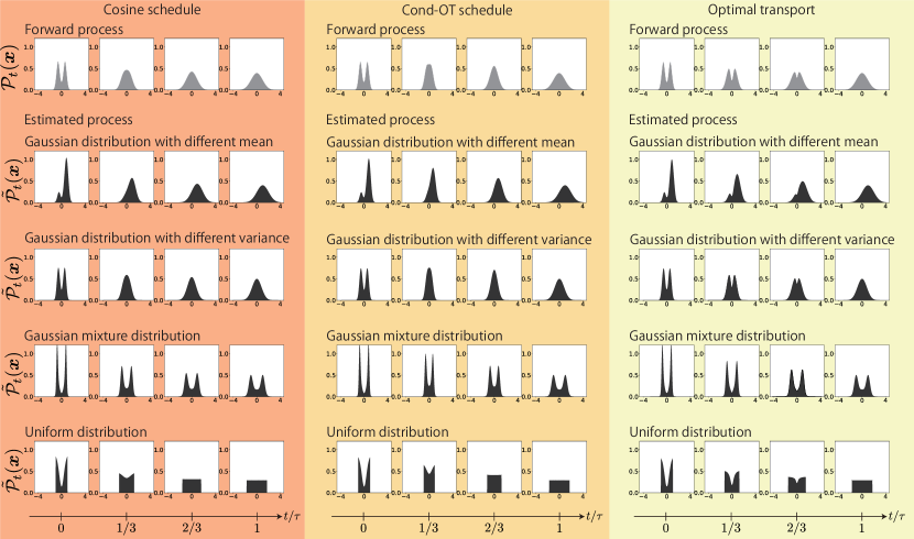
Figure 5: The time evolution of the probability density functions in the forward and estimated processes, for each condition used in the numerical calculations [Fig. 4].

References

- Van Kampen [1992] N. G. Van Kampen, Stochastic processes in physics and chemistry, Vol. 1 (Elsevier, 1992).
- Sekimoto [2010] K. Sekimoto, Stochastic energetics (2010).
- Seifert [2012] U. Seifert, Stochastic thermodynamics, fluctuation theorems and molecular machines, Reports on progress in physics 75, 126001 (2012).
- Sekimoto [1998] K. Sekimoto, Langevin equation and thermodynamics, Progress of Theoretical Physics Supplement 130, 17 (1998).
- Kurchan [1998] J. Kurchan, Fluctuation theorem for stochastic dynamics, Journal of Physics A: Mathematical and General 31, 3719 (1998).
- Hatano and Sasa [2001] T. Hatano and S.-i. Sasa, Steady-state thermodynamics of langevin systems, Physical review letters 86, 3463 (2001).
- Seifert [2005] U. Seifert, Entropy production along a stochastic trajectory and an integral fluctuation theorem, Physical review letters 95, 040602 (2005).
- Chernyak et al. [2006] V. Y. Chernyak, M. Chertkov, and C. Jarzynski, Path-integral analysis of fluctuation theorems for general langevin processes, Journal of Statistical Mechanics: Theory and Experiment 2006, P08001 (2006).
- Schmiedl and Seifert [2007] T. Schmiedl and U. Seifert, Efficiency at maximum power: An analytically solvable model for stochastic heat engines, Europhysics letters 81, 20003 (2007).
- Allahverdyan et al. [2009] A. E. Allahverdyan, D. Janzing, and G. Mahler, Thermodynamic efficiency of information and heat flow, Journal of Statistical Mechanics: Theory and Experiment 2009, P09011 (2009).
- Van den Broeck and Esposito [2010] C. Van den Broeck and M. Esposito, Three faces of the second law. ii. fokker-planck formulation, Physical Review E 82, 011144 (2010).
- Sagawa and Ueda [2012] T. Sagawa and M. Ueda, Nonequilibrium thermodynamics of feedback control, Physical Review E 85, 021104 (2012).
- Ito and Sagawa [2013] S. Ito and T. Sagawa, Information thermodynamics on causal networks, Physical review letters 111, 180603 (2013).
- Horowitz and Sandberg [2014] J. M. Horowitz and H. Sandberg, Second-law-like inequalities with information and their interpretations, New Journal of Physics 16, 125007 (2014).
- Ito and Sagawa [2015] S. Ito and T. Sagawa, Maxwell’s demon in biochemical signal transduction with feedback loop, Nature communications 6, 1 (2015).
- Gingrich et al. [2017] T. R. Gingrich, G. M. Rotskoff, and J. M. Horowitz, Inferring dissipation from current fluctuations, Journal of Physics A: Mathematical and Theoretical 50, 184004 (2017).
- Dechant and Sasa [2018] A. Dechant and S.-i. Sasa, Entropic bounds on currents in langevin systems, Physical Review E 97, 062101 (2018).
- Li et al. [2019] J. Li, J. M. Horowitz, T. R. Gingrich, and N. Fakhri, Quantifying dissipation using fluctuating currents, Nature communications 10, 1666 (2019).
- Hasegawa and Van Vu [2019] Y. Hasegawa and T. Van Vu, Uncertainty relations in stochastic processes: An information inequality approach, Physical Review E 99, 062126 (2019).
- Ito and Dechant [2020] S. Ito and A. Dechant, Stochastic time evolution, information geometry, and the cramér-rao bound, Physical Review X 10, 021056 (2020).
- Otsubo et al. [2020] S. Otsubo, S. Ito, A. Dechant, and T. Sagawa, Estimating entropy production by machine learning of short-time fluctuating currents, Physical Review E 101, 062106 (2020).
- Dechant and Sasa [2021] A. Dechant and S.-i. Sasa, Continuous time reversal and equality in the thermodynamic uncertainty relation, Physical Review Research 3, L042012 (2021).
- Otsubo et al. [2022] S. Otsubo, S. K. Manikandan, T. Sagawa, and S. Krishnamurthy, Estimating time-dependent entropy production from non-equilibrium trajectories, Communications Physics 5, 11 (2022).
- Koyuk and Seifert [2020] T. Koyuk and U. Seifert, Thermodynamic uncertainty relation for time-dependent driving, Physical Review Letters 125, 260604 (2020).
- Villani et al. [2009] C. Villani et al., Optimal transport: old and new, Vol. 338 (Springer, 2009).
- Jordan et al. [1998] R. Jordan, D. Kinderlehrer, and F. Otto, The variational formulation of the fokker–planck equation, SIAM journal on mathematical analysis 29, 1 (1998).
- Aurell et al. [2011] E. Aurell, C. Mejía-Monasterio, and P. Muratore-Ginanneschi, Optimal protocols and optimal transport in stochastic thermodynamics, Physical review letters 106, 250601 (2011).
- Chen et al. [2019] Y. Chen, T. T. Georgiou, and A. Tannenbaum, Stochastic control and nonequilibrium thermodynamics: Fundamental limits, IEEE transactions on automatic control 65, 2979 (2019).
- Nakazato and Ito [2021] M. Nakazato and S. Ito, Geometrical aspects of entropy production in stochastic thermodynamics based on wasserstein distance, Physical Review Research 3, 043093 (2021).
- Aurell et al. [2012] E. Aurell, K. Gawȩdzki, C. Mejía-Monasterio, R. Mohayaee, and P. Muratore-Ginanneschi, Refined second law of thermodynamics for fast random processes, Journal of Statistical Physics 147, 487 (2012).
- Dechant et al. [2022a] A. Dechant, S.-i. Sasa, and S. Ito, Geometric decomposition of entropy production into excess, housekeeping, and coupling parts, Physical Review E 106, 024125 (2022a).
- Ito [2024] S. Ito, Geometric thermodynamics for the fokker–planck equation: stochastic thermodynamic links between information geometry and optimal transport, Information Geometry 7, 441 (2024).
- Nagayama et al. [2023] R. Nagayama, K. Yoshimura, A. Kolchinsky, and S. Ito, Geometric thermodynamics of reaction-diffusion systems: Thermodynamic trade-off relations and optimal transport for pattern formation, arXiv preprint arXiv:2311.16569 (2023).
- Tomczak [2022] J. M. Tomczak, Deep generative modeling (Springer, 2022).
- Sohl-Dickstein et al. [2015] J. Sohl-Dickstein, E. Weiss, N. Maheswaranathan, and S. Ganguli, Deep unsupervised learning using nonequilibrium thermodynamics, in International conference on machine learning (PMLR, 2015) pp. 2256–2265.
- Song et al. [2020a] Y. Song, J. Sohl-Dickstein, D. P. Kingma, A. Kumar, S. Ermon, and B. Poole, Score-based generative modeling through stochastic differential equations, in International Conference on Learning Representations (2020).
- Evans and Searles [2002] D. J. Evans and D. J. Searles, The fluctuation theorem, Advances in Physics 51, 1529 (2002).
- Crooks [1999] G. E. Crooks, Entropy production fluctuation theorem and the nonequilibrium work relation for free energy differences, Physical Review E 60, 2721 (1999).
- Jarzynski [1997] C. Jarzynski, Nonequilibrium equality for free energy differences, Physical Review Letters 78, 2690 (1997).
- Ho et al. [2020] J. Ho, A. Jain, and P. Abbeel, Denoising diffusion probabilistic models, Advances in neural information processing systems 33, 6840 (2020).
- Kingma et al. [2021] D. Kingma, T. Salimans, B. Poole, and J. Ho, Variational diffusion models, Advances in neural information processing systems 34, 21696 (2021).
- Song and Ermon [2019] Y. Song and S. Ermon, Generative modeling by estimating gradients of the data distribution, Advances in neural information processing systems 32 (2019).
- Nichol and Dhariwal [2021] A. Q. Nichol and P. Dhariwal, Improved denoising diffusion probabilistic models, in International Conference on Machine Learning (PMLR, 2021) pp. 8162–8171.
- Rombach et al. [2022] R. Rombach, A. Blattmann, D. Lorenz, P. Esser, and B. Ommer, High-resolution image synthesis with latent diffusion models, in Proceedings of the IEEE/CVF conference on computer vision and pattern recognition (2022) pp. 10684–10695.
- Song and Ermon [2020] Y. Song and S. Ermon, Improved techniques for training score-based generative models, Advances in neural information processing systems 33, 12438 (2020).
- Song et al. [2023] Y. Song, P. Dhariwal, M. Chen, and I. Sutskever, Consistency models, arXiv preprint arXiv:2303.01469 (2023).
- Dhariwal and Nichol [2021] P. Dhariwal and A. Nichol, Diffusion models beat gans on image synthesis, Advances in neural information processing systems 34, 8780 (2021).
- Song et al. [2020b] J. Song, C. Meng, and S. Ermon, Denoising diffusion implicit models, in International Conference on Learning Representations (2020).
- Karras et al. [2022] T. Karras, M. Aittala, T. Aila, and S. Laine, Elucidating the design space of diffusion-based generative models, Advances in Neural Information Processing Systems 35, 26565 (2022).
- Chen et al. [2021] T. Chen, G.-H. Liu, and E. Theodorou, Likelihood training of schrödinger bridge using forward-backward sdes theory, in International Conference on Learning Representations (2021).
- Ramesh et al. [2022] A. Ramesh, P. Dhariwal, A. Nichol, C. Chu, and M. Chen, Hierarchical text-conditional image generation with clip latents, arXiv preprint arXiv:2204.06125 1, 3 (2022).
- Ho and Salimans [2022] J. Ho and T. Salimans, Classifier-free diffusion guidance, arXiv preprint arXiv:2207.12598 (2022).
- Nichol et al. [2021] A. Nichol, P. Dhariwal, A. Ramesh, P. Shyam, P. Mishkin, B. McGrew, I. Sutskever, and M. Chen, Glide: Towards photorealistic image generation and editing with text-guided diffusion models, arXiv preprint arXiv:2112.10741 (2021).
- Sauer et al. [2024] A. Sauer, F. Boesel, T. Dockhorn, A. Blattmann, P. Esser, and R. Rombach, Fast high-resolution image synthesis with latent adversarial diffusion distillation, arXiv preprint arXiv:2403.12015 (2024).
- Podell et al. [2023] D. Podell, Z. English, K. Lacey, A. Blattmann, T. Dockhorn, J. Müller, J. Penna, and R. Rombach, Sdxl: Improving latent diffusion models for high-resolution image synthesis, arXiv preprint arXiv:2307.01952 (2023).
- Hyvärinen and Dayan [2005] A. Hyvärinen and P. Dayan, Estimation of non-normalized statistical models by score matching., Journal of Machine Learning Research 6 (2005).
- Vincent [2011] P. Vincent, A connection between score matching and denoising autoencoders, Neural computation 23, 1661 (2011).
- Kingma and Cun [2010] D. P. Kingma and Y. Cun, Regularized estimation of image statistics by score matching, Advances in neural information processing systems 23 (2010).
- Dinh et al. [2014] L. Dinh, D. Krueger, and Y. Bengio, Nice: Non-linear independent components estimation, arXiv preprint arXiv:1410.8516 (2014).
- Rezende and Mohamed [2015] D. Rezende and S. Mohamed, Variational inference with normalizing flows, in International conference on machine learning (PMLR, 2015) pp. 1530–1538.
- Chen et al. [2018] R. T. Chen, Y. Rubanova, J. Bettencourt, and D. K. Duvenaud, Neural ordinary differential equations, Advances in neural information processing systems 31 (2018).
- Song [2022] K.-U. Song, Applying regularized schr” odinger-bridge-based stochastic process in generative modeling, arXiv preprint arXiv:2208.07131 (2022).
- Lipman et al. [2022] Y. Lipman, R. T. Chen, H. Ben-Hamu, M. Nickel, and M. Le, Flow matching for generative modeling, in The Eleventh International Conference on Learning Representations (2022).
- Arjovsky et al. [2017] M. Arjovsky, S. Chintala, and L. Bottou, Wasserstein generative adversarial networks, in International conference on machine learning (PMLR, 2017) pp. 214–223.
- Kwon et al. [2022] D. Kwon, Y. Fan, and K. Lee, Score-based generative modeling secretly minimizes the wasserstein distance, Advances in Neural Information Processing Systems 35, 20205 (2022).
- Oko et al. [2023] K. Oko, S. Akiyama, and T. Suzuki, Diffusion models are minimax optimal distribution estimators, in International Conference on Machine Learning (PMLR, 2023) pp. 26517–26582.
- De Bortoli [2022] V. De Bortoli, Convergence of denoising diffusion models under the manifold hypothesis, arXiv preprint arXiv:2208.05314 (2022).
- Kornilov et al. [2024] N. Kornilov, A. Gasnikov, and A. Korotin, Optimal flow matching: Learning straight trajectories in just one step, arXiv preprint arXiv:2403.13117 (2024).
- Shaul et al. [2023] N. Shaul, R. T. Chen, M. Nickel, M. Le, and Y. Lipman, On kinetic optimal probability paths for generative models, in International Conference on Machine Learning (PMLR, 2023) pp. 30883–30907.
- Tong et al. [2023] A. Tong, N. Malkin, G. Huguet, Y. Zhang, J. Rector-Brooks, K. Fatras, G. Wolf, and Y. Bengio, Improving and generalizing flow-based generative models with minibatch optimal transport, in ICML Workshop on New Frontiers in Learning, Control, and Dynamical Systems (2023).
- Shi et al. [2022] Y. Shi, V. De Bortoli, G. Deligiannidis, and A. Doucet, Conditional simulation using diffusion schrödinger bridges, in Uncertainty in Artificial Intelligence (PMLR, 2022) pp. 1792–1802.
- Liu et al. [2022] X. Liu, C. Gong, and Q. Liu, Flow straight and fast: Learning to generate and transfer data with rectified flow, arXiv preprint arXiv:2209.03003 (2022).
- Esser et al. [2024] P. Esser, S. Kulal, A. Blattmann, R. Entezari, J. Müller, H. Saini, Y. Levi, D. Lorenz, A. Sauer, F. Boesel, et al., Scaling rectified flow transformers for high-resolution image synthesis, arXiv preprint arXiv:2403.03206 (2024).
- Klinger and Rotskoff [2024] J. Klinger and G. M. Rotskoff, Universal energy-speed-accuracy trade-offs in driven nonequilibrium systems (2024), arXiv:2402.17931 [cond-mat.stat-mech] .
- Brock et al. [2018] A. Brock, J. Donahue, and K. Simonyan, Large scale gan training for high fidelity natural image synthesis, arXiv preprint arXiv:1809.11096 (2018).
- Brown et al. [2020] T. Brown, B. Mann, N. Ryder, M. Subbiah, J. D. Kaplan, P. Dhariwal, A. Neelakantan, P. Shyam, G. Sastry, A. Askell, et al., Language models are few-shot learners, Advances in neural information processing systems 33, 1877 (2020).
- Oord et al. [2016] A. v. d. Oord, S. Dieleman, H. Zen, K. Simonyan, O. Vinyals, A. Graves, N. Kalchbrenner, A. Senior, and K. Kavukcuoglu, Wavenet: A generative model for raw audio, arXiv preprint arXiv:1609.03499 (2016).
- Goodfellow et al. [2016] I. Goodfellow, Y. Bengio, and A. Courville, Deep Learning (MIT Press, 2016).
- Theis et al. [2015] L. Theis, A. v. d. Oord, and M. Bethge, A note on the evaluation of generative models, arXiv preprint arXiv:1511.01844 (2015).
- Betzalel et al. [2022] E. Betzalel, C. Penso, A. Navon, and E. Fetaya, A study on the evaluation of generative models, arXiv preprint arXiv:2206.10935 (2022).
- Bischoff et al. [2024] S. Bischoff, A. Darcher, M. Deistler, R. Gao, F. Gerken, M. Gloeckler, L. Haxel, J. Kapoor, J. K. Lappalainen, J. H. Macke, et al., A practical guide to statistical distances for evaluating generative models in science, arXiv preprint arXiv:2403.12636 (2024).
- Heusel et al. [2017] M. Heusel, H. Ramsauer, T. Unterthiner, B. Nessler, and S. Hochreiter, Gans trained by a two time-scale update rule converge to a local nash equilibrium, Advances in neural information processing systems 30 (2017).
- Amari [2016] S.-i. Amari, Information geometry and its applications, Vol. 194 (Springer, 2016).
- Poole et al. [2022] B. Poole, A. Jain, J. T. Barron, and B. Mildenhall, Dreamfusion: Text-to-3d using 2d diffusion, arXiv preprint arXiv:2209.14988 (2022).
- Xu et al. [2022] M. Xu, L. Yu, Y. Song, C. Shi, S. Ermon, and J. Tang, Geodiff: A geometric diffusion model for molecular conformation generation, arXiv preprint arXiv:2203.02923 (2022).
- Abramson et al. [2024] J. Abramson, J. Adler, J. Dunger, R. Evans, T. Green, A. Pritzel, O. Ronneberger, L. Willmore, A. J. Ballard, J. Bambrick, et al., Accurate structure prediction of biomolecular interactions with alphafold 3, Nature , 1 (2024).
- Ho et al. [2022] J. Ho, W. Chan, C. Saharia, J. Whang, R. Gao, A. Gritsenko, D. P. Kingma, B. Poole, M. Norouzi, D. J. Fleet, et al., Imagen video: High definition video generation with diffusion models, arXiv preprint arXiv:2210.02303 (2022).
- Brooks et al. [2024] T. Brooks, B. Peebles, C. Holmes, W. DePue, Y. Guo, L. Jing, D. Schnurr, J. Taylor, T. Luhman, E. Luhman, C. Ng, R. Wang, and A. Ramesh, Video generation models as world simulators, (2024).
- Chen et al. [2020] N. Chen, Y. Zhang, H. Zen, R. J. Weiss, M. Norouzi, and W. Chan, Wavegrad: Estimating gradients for waveform generation, in International Conference on Learning Representations (2020).
- Kong et al. [2020] Z. Kong, W. Ping, J. Huang, K. Zhao, and B. Catanzaro, Diffwave: A versatile diffusion model for audio synthesis, in International Conference on Learning Representations (2020).
- [91] Smithsonian butterflies subset, accessed: 2024-02-09.
- Risken and Risken [1996] H. Risken and H. Risken, Fokker-planck equation (Springer, 1996).
- Van Kampen [1976] N. G. Van Kampen, Stochastic differential equations, Physics reports 24, 171 (1976).
- Brooks [1998] S. Brooks, Markov chain monte carlo method and its application, Journal of the royal statistical society: series D (the Statistician) 47, 69 (1998).
- Andrieu et al. [2003] C. Andrieu, N. De Freitas, A. Doucet, and M. I. Jordan, An introduction to mcmc for machine learning, Machine learning 50, 5 (2003).
- Welling and Teh [2011] M. Welling and Y. W. Teh, Bayesian learning via stochastic gradient langevin dynamics, in Proceedings of the 28th international conference on machine learning (ICML-11) (Citeseer, 2011) pp. 681–688.
- Chen [2023] T. Chen, On the importance of noise scheduling for diffusion models, arXiv preprint arXiv:2301.10972 (2023).
- Anderson [1982] B. D. Anderson, Reverse-time diffusion equation models, Stochastic Processes and their Applications 12, 313 (1982).
- Lu et al. [2022a] C. Lu, Y. Zhou, F. Bao, J. Chen, C. Li, and J. Zhu, Dpm-solver: A fast ode solver for diffusion probabilistic model sampling in around 10 steps, Advances in Neural Information Processing Systems 35, 5775 (2022a).
- Lu et al. [2022b] C. Lu, K. Zheng, F. Bao, J. Chen, C. Li, and J. Zhu, Maximum likelihood training for score-based diffusion odes by high order denoising score matching, in International Conference on Machine Learning (PMLR, 2022) pp. 14429–14460.
- Zhang and Chen [2022] Q. Zhang and Y. Chen, Fast sampling of diffusion models with exponential integrator, arXiv preprint arXiv:2204.13902 (2022).
- Kobyzev et al. [2020] I. Kobyzev, S. J. Prince, and M. A. Brubaker, Normalizing flows: An introduction and review of current methods, IEEE transactions on pattern analysis and machine intelligence 43, 3964 (2020).
- Ito et al. [2020] S. Ito, M. Oizumi, and S.-i. Amari, Unified framework for the entropy production and the stochastic interaction based on information geometry, Physical Review Research 2, 033048 (2020).
- Kawai et al. [2007] R. Kawai, J. M. Parrondo, and C. Van den Broeck, Dissipation: The phase-space perspective, Physical review letters 98, 080602 (2007).
- Villani [2021] C. Villani, Topics in optimal transportation, Vol. 58 (American Mathematical Soc., 2021).
- Givens and Shortt [1984] C. R. Givens and R. M. Shortt, A class of wasserstein metrics for probability distributions, Michigan Mathematical Journal 31, 231 (1984).
- Benamou and Brenier [2000] J.-D. Benamou and Y. Brenier, A computational fluid mechanics solution to the monge-kantorovich mass transfer problem, Numerische Mathematik 84, 375 (2000).
- Dechant et al. [2022b] A. Dechant, S.-i. Sasa, and S. Ito, Geometric decomposition of entropy production in out-of-equilibrium systems, Physical Review Research 4, L012034 (2022b).
- Benamou and Brenier [1999] J.-D. Benamou and Y. Brenier, A numerical method for the optimal time-continuous mass transport problem and related problems, Contemporary mathematics 226, 1 (1999).
- Sekizawa et al. [2023] D. Sekizawa, S. Ito, and M. Oizumi, Decomposing thermodynamic dissipation of neural dynamics via spatio-temporal oscillatory modes, arXiv preprint arXiv:2312.03489 (2023).
- Crooks [2000] G. E. Crooks, Path-ensemble averages in systems driven far from equilibrium, Physical review E 61, 2361 (2000).
- Horowitz and Gingrich [2020] J. M. Horowitz and T. R. Gingrich, Thermodynamic uncertainty relations constrain non-equilibrium fluctuations, Nature Physics 16, 15 (2020).
- Pearson [1900] K. Pearson, X. on the criterion that a given system of deviations from the probable in the case of a correlated system of variables is such that it can be reasonably supposed to have arisen from random sampling, The London, Edinburgh, and Dublin Philosophical Magazine and Journal of Science 50, 157 (1900).
- Barato and Seifert [2015] A. C. Barato and U. Seifert, Thermodynamic uncertainty relation for biomolecular processes, Physical review letters 114, 158101 (2015).
- Dechant [2022] A. Dechant, Minimum entropy production, detailed balance and wasserstein distance for continuous-time markov processes, Journal of Physics A: Mathematical and Theoretical 55, 094001 (2022).
- Yoshimura et al. [2023] K. Yoshimura, A. Kolchinsky, A. Dechant, and S. Ito, Housekeeping and excess entropy production for general nonlinear dynamics, Physical Review Research 5, 013017 (2023).
- Van Vu and Saito [2023] T. Van Vu and K. Saito, Thermodynamic unification of optimal transport: Thermodynamic uncertainty relation, minimum dissipation, and thermodynamic speed limits, Physical Review X 13, 011013 (2023).
- Kolchinsky et al. [2022] A. Kolchinsky, A. Dechant, K. Yoshimura, and S. Ito, Information geometry of excess and housekeeping entropy production, arXiv preprint arXiv:2206.14599 (2022).
- Wang et al. [2021] G. Wang, Y. Jiao, Q. Xu, Y. Wang, and C. Yang, Deep generative learning via schrödinger bridge, in International conference on machine learning (PMLR, 2021) pp. 10794–10804.
- De Bortoli et al. [2021] V. De Bortoli, J. Thornton, J. Heng, and A. Doucet, Diffusion schrödinger bridge with applications to score-based generative modeling, Advances in Neural Information Processing Systems 34, 17695 (2021).
- Song et al. [2021] Y. Song, C. Durkan, I. Murray, and S. Ermon, Maximum likelihood training of score-based diffusion models, Advances in neural information processing systems 34, 1415 (2021).
- Lee et al. [2022] H. Lee, J. Lu, and Y. Tan, Convergence for score-based generative modeling with polynomial complexity, Advances in Neural Information Processing Systems 35, 22870 (2022).
- Chen et al. [2023] S. Chen, S. Chewi, J. Li, Y. Li, A. Salim, and A. R. Zhang, Sampling is as easy as learning the score: theory for diffusion models with minimal data assumptions, in International Conference on Learning Representations (2023).
- Albergo and Vanden-Eijnden [2022] M. S. Albergo and E. Vanden-Eijnden, Building normalizing flows with stochastic interpolants, arXiv preprint arXiv:2209.15571 (2022).
- Pooladian et al. [2023] A. A. Pooladian, H. Ben-Hamu, C. Domingo-Enrich, B. Amos, Y. Lipman, and R. T. Chen, Multisample flow matching: Straightening flows with minibatch couplings, Proceedings of Machine Learning Research 202, 28100 (2023).
- Flamary et al. [2021] R. Flamary, N. Courty, A. Gramfort, M. Z. Alaya, A. Boisbunon, S. Chambon, L. Chapel, A. Corenflos, K. Fatras, N. Fournier, et al., Pot: Python optimal transport, Journal of Machine Learning Research 22, 1 (2021).
- Kingma and Ba [2015] D. Kingma and J. Ba, Adam: A method for stochastic optimization, in International Conference on Learning Representations (2015).
- Kutta [1901] W. Kutta, Beitrag zur näherungsweisen Integration totaler Differentialgleichungen (Teubner, 1901).