Quantal phase of extreme nonstatic light waves: Step-phase evolution and its effects
Abstract
The phases are the main factor that affects the outcome of various optical phenomena, such as
quantum superposition, wave interference, and light–matter interaction.
As a light wave becomes nonstatic, an additional phase, the so-called geometric phase, takes
place in its evolution. Then, due to this phase, the overall phase of the
quantum wave function varies in a nonlinear way with time.
Interestingly,
the phase exhibits a step-like evolution if the measure of nonstaticity is extremely high.
Such an abnormal phase variation
is analyzed in detail for better understanding of wave nonstaticity in this work.
As the wave becomes highly nonstatic, the phase factor of the electromagnetic wave
evolves in a rectangular manner.
However, the shape of the electromagnetic field is still a sinusoidal form
on account of the compensational variation of the wave amplitude.
The electromagnetic field in this case very much resembles that of a standing wave.
The effects accompanying the step-phase evolution, such as modification
of the probability distribution and alteration of the wave-interference profile,
are analyzed and their implications are illustrated.
1. INTRODUCTION
If the parameters of a medium vary in time, the waves which propagate through it become
nonstatic according to the Maxwell’s electromagnetic theory.
However, in the previous works nwh ; gow ; ncs ; gch , we have shown that
nonstatic quantum waves can also take place even when the medium
is transparent and its parameters do not vary.
Such nonstatic waves exhibit a peculiar time behavior, which is that
the waves expand and shrink in turn periodically in the quadrature space.
While the above interpretation for nonstatic-wave evolution is based on the exact solutions of the Schrödinger wave equation, we still do not know much about the properties of the nonstatic waves arisen in a static environment. Many physical characteristics of the nonstatic light may long for clarification yet. Especially, the behavior of highly nonstatic waves may greatly deviate from that of the ordinary ones.
In this work, we are interested in the phases accompanied the quantum wave functions of nonstatic light. In order to interpret quantum mechanics based on particle-wave duality and non-locality, it is necessary to know the fundamental relation between quantum wave phase and the associated physical reality kop . For decades, considerable research has been devoted to phase sensitive experiments with the waves that undergo intraatomic/intramolecular propagation spe1 ; spe2 ; spe4 ; spe5 , as well as free wave-packets. The development of techniques for controlling and manipulating quantum phases may open a new route for a variety of their applications, for example, in wireless communications wc1 ; wc2 , tunable optical devices tod , beam forming and scanning bfs-0 ; bfs , radar detection rad , and biological monitoring bmo1 ; bmo2 .
We know that the phase of an ordinary quantum wave in free space evolves monotonically in time. However, if a wave becomes nonstatic, the behavior of the phase is not so simple because there appears an additional phase (geometric phase) which shows the geometry in the evolution of the wave gow ; gch . The wave phase not only directly affects the electromagnetic wave phenomena, but is responsible for a distinguishable change of the interference picture in an electromagnetic interaction bfs ; rem . In particular, the nature of the electromagnetic fields in the near-field, including their phase properties, is very different from that of the far-field in free space nef ; nrp . Moreover, a perturbation of near-fields leads to a modification of overall phases in addition to the change of the polarization and wave intensity cpe . Superposition of quantum states is also governed by the phases of its constituent substates. The change in the probability distributions for superposition states in Hilbert space, caused for example by the nonstaticity-induced geometric phase, is noteworthy in connection with diverse phase-related quantum technologies gpp3 ; gpp4 ; gpp5 ; gpp7 .
Phases properties of the nonstatic quantum waves are analyzed in this work,
focusing especially on highly nonstatic waves.
We show that the phase evolves in a novel step-like way in time
in the limit of an extreme nonstaticity.
The associated consequences
in the wave phenomena, such as electromagnetic wave propagation, superposition of quantum
states, and wave interference, are investigated rigorously.
Physical meanings of the emergence of the abnormal step
phase are interpreted from a fundamental quantum point of view.
2. OUTLINE FOR STEP-LIKE PHASE EVOLUTION
In this section, we see how nonstaticity of a light wave affects the properties of its phase.
The phase of a wave plays a crucial role in the description of
wave propagation, interference patterns, and quantum superpositions.
It is expected that the phase properties of nonstatic waves are
extraordinary due to the appearance of the geometric phase.
In particular, the physical characteristics of highly nonstatic waves and their quantal phases
may be significantly different from the usually known ones.
The actual electromagnetic fields are described in a complicated way via the functions of both space and time even in free space cme2 ; cme3 . Wave nonstaticity is also a factor that makes the wave representation being complicated. To see the effects of wave nonstaticity on phase properties, we start from the formula of the general wave functions for plane waves in a source free region. The wave functions for such a light wave in the Fock states are given by
| (1) |
where are the eigenfunctions and are the phases of the wave. For a nonstatic wave, the phases are expressed as nwh ; gow
| (2) |
| (3) |
where is a time function of the form
| (4) |
while , and are real constants. Additionally, the coefficients in Eq. (4) obey the conditions and . For , the phase given in Eq. (2) is the same as that in the coherent state gch .
Let us restrict the range of in a cycle without loss of generality, such that . Then, from the integration given in Eq. (3), we have ncs
| (5) |
for , where , , and is the unit step function (Heaviside step function). Although our research in this work is focused on phase properties of the wave functions, the eigenfunctions in Eq. (1) have also been represented in Appendix A for completeness.
Basically, we are interested in the phase of a highly nonstatic wave. The degree of wave nonstaticity can be estimated from the measure of nonstaticity that has been represented in Appendix B. The scale of nonstaticity of a wave increases as grows. The wave nonstaticity is actually governed by the values of and , because is represented in terms of them as can be seen from Eq. (23) in Appendix B.
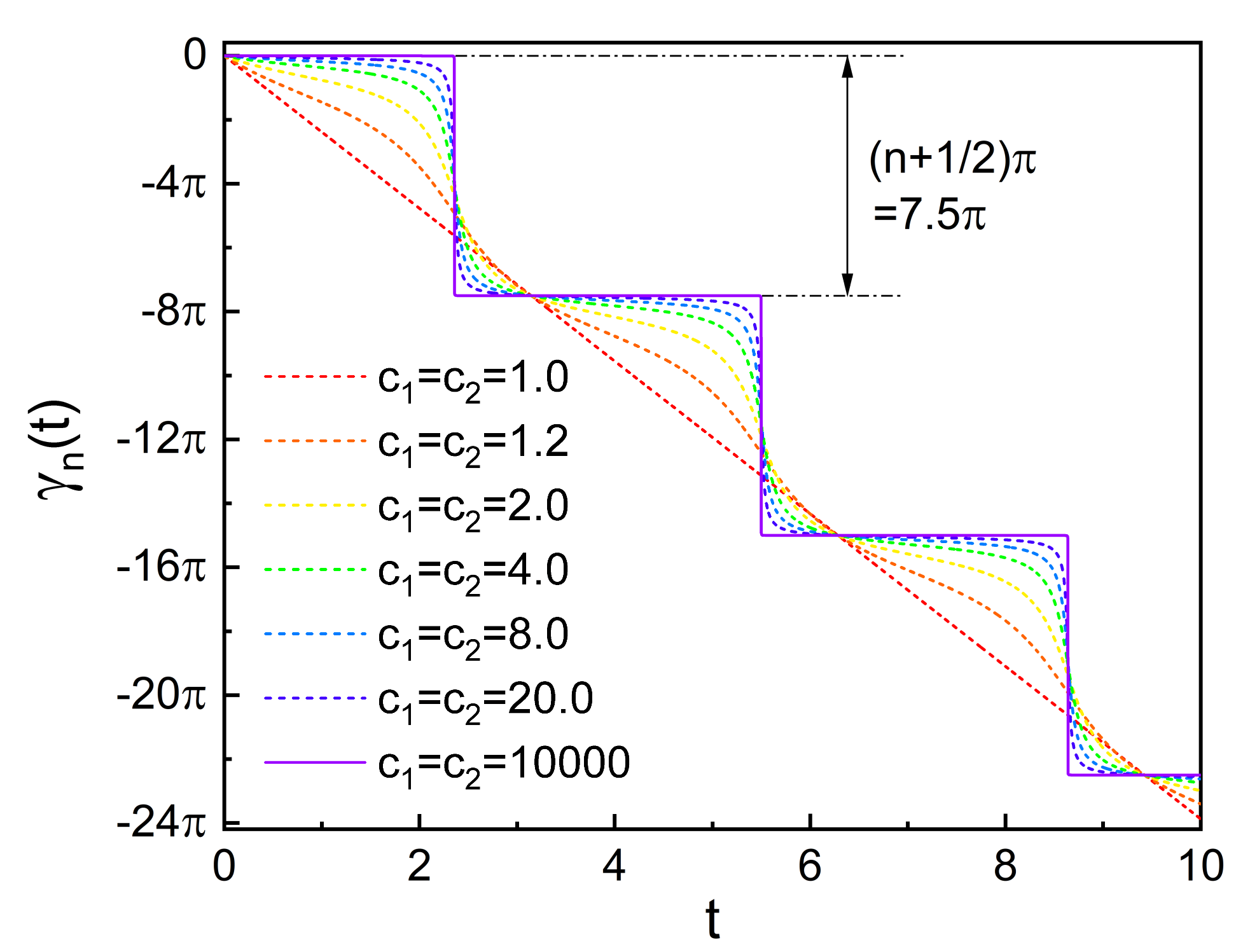
Equation (2) is the same as the addition of the dynamical and geometric phases shown in Appendix C. The behavior of this phase when the wave nonstaticity is non-negligible may be notable due to its characteristic abnormal properties. Figure 1 exhibits the change of the pattern for the time evolution of the phase as the degree of nonstaticity increases. Except for the case which corresponds to the static wave, the phase evolution is nonlinear. The scale of such a nonlinearity is gradually augmented as the measure of nonstaticity increases. Eventually, when the nonstaticity measure is extremely large, the quantum phase exhibits a step-like time behavior, which drops periodically. This is closely related to the time variation of the eigenfunctions given in Eq. (22) in Appendix A and the appearing of additional phases (the geometric phases) as the wave becomes nonstatic. The change of phase in each drop in a Fock state is as shown in Fig. 1.
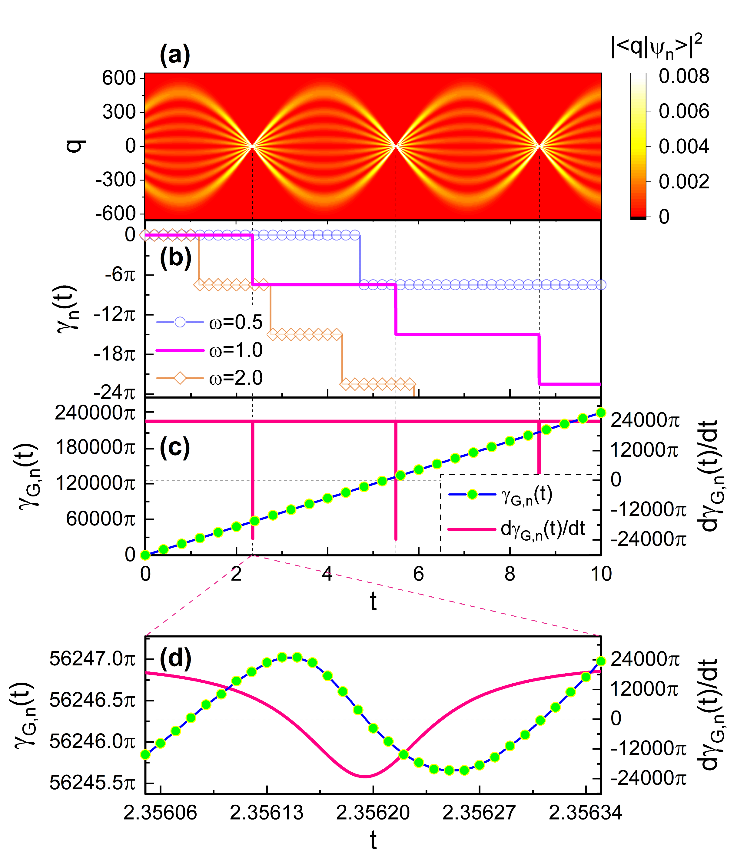
Figure 2 shows that the quantum phase precipitates whenever the probability density
constitutes a node during its time evolution in the quadrature space.
At a glance, it seems that the geometric phase depicted in Fig. 2(c) increases linearly over time.
However, it is not the case gow .
We can see from Fig. 2(d) that the geometric phase undergoes a nontrivial nonlinear variation during
a negligibly short time.
This consequence can also be confirmed from the periodical abrupt change of the gradient of the
geometric phase, which is shown in Figs. 2(c) and 2(d) with the red curve.
This extremal behavior of the geometric phase is the extension of the usual consequence for
the nonstaticity-induced geometric phase (shown in Ref. gow ) to an extremely higher nonstatic case.
3. DESCRIPTION OF NONSTATIC ELECTROMAGNETIC FIELDS
The analysis of spatiotemporal evolution of nonstatic light of which phase exhibits nonlinear properties
is necessary for the understanding of the propagation of such an unusual light wave.
This analysis also helps the conceptualization and characterization of
correlated coherent states for nonstatic waves, including interpreting of
the related quantum measurements.
Let us see the effects of the characteristic phase evolution for a highly nonstatic coherent wave on its propagation. The coherent state for a nonstatic wave is obtained by means of a generalized annihilation operator. From the definition of such an annihilation operator in the nonstatic regime, which is
| (6) |
| (7) |
where is a constant. In particular, for , this reduces to . From the eigenvalue equation the eigenvalue is obtained in the form ncs
| (8) |
where is an amplitude which is real. This preliminary description for the annihilation operator and its eigenvalue will be used later in order to unfold the theory of nonstatic coherent waves.
To see the effects of wave nonstaticity on the evolution of electromagnetic waves, we regard the associated vector potential. Since the vector potential is a sum of its components of each radiation mode whl , it reads
| (9) |
where is a shorthand notation for with , is the position function and is the amplitude for mode . We consider a plane wave which propagates with a periodic boundary condition, . Then, the position and time functions are represented, respectively, as
| (10) |
| (11) |
where the wave vector is of the form , is the speed of light in the medium, are two unit vectors associated with the polarization direction, and . Then, the mode of the polarization is completely given from the set (, , , ).
By considering only a particular mode frequency with a polarization, let us drop the subscripts and from now on for convenience. Then, the vector potential can be written such that
| (12) |
For the purpose of further simplicity, we now consider the case that the wave propagates direction. Then the vector potential is reduced to
| (13) |
where . In the derivation of Eq. (13), we used the formula given in Eq. (8).
The electric and magnetic fields in the source-free space can be obtained solely from the expression of via the relations
| (14) | |||
| (15) |
To evaluate these equations for the wave propagating through direction, we insert Eq. (13) into Eqs. (14) and (15). This procedure results in
| (16) | |||||
| (17) |
where , ,
, and .
Here, is the inverse function of
defined within a cycle of the angle, .
4. SPATIOTEMPORAL EVOLUTION OF NONSTATIC WAVES
4.1. Analysis of mechanism for emerging nonstaticity
Let us see the mechanism of appearing nonstaticity in electric field in this subsection using the development
given in the previous section.
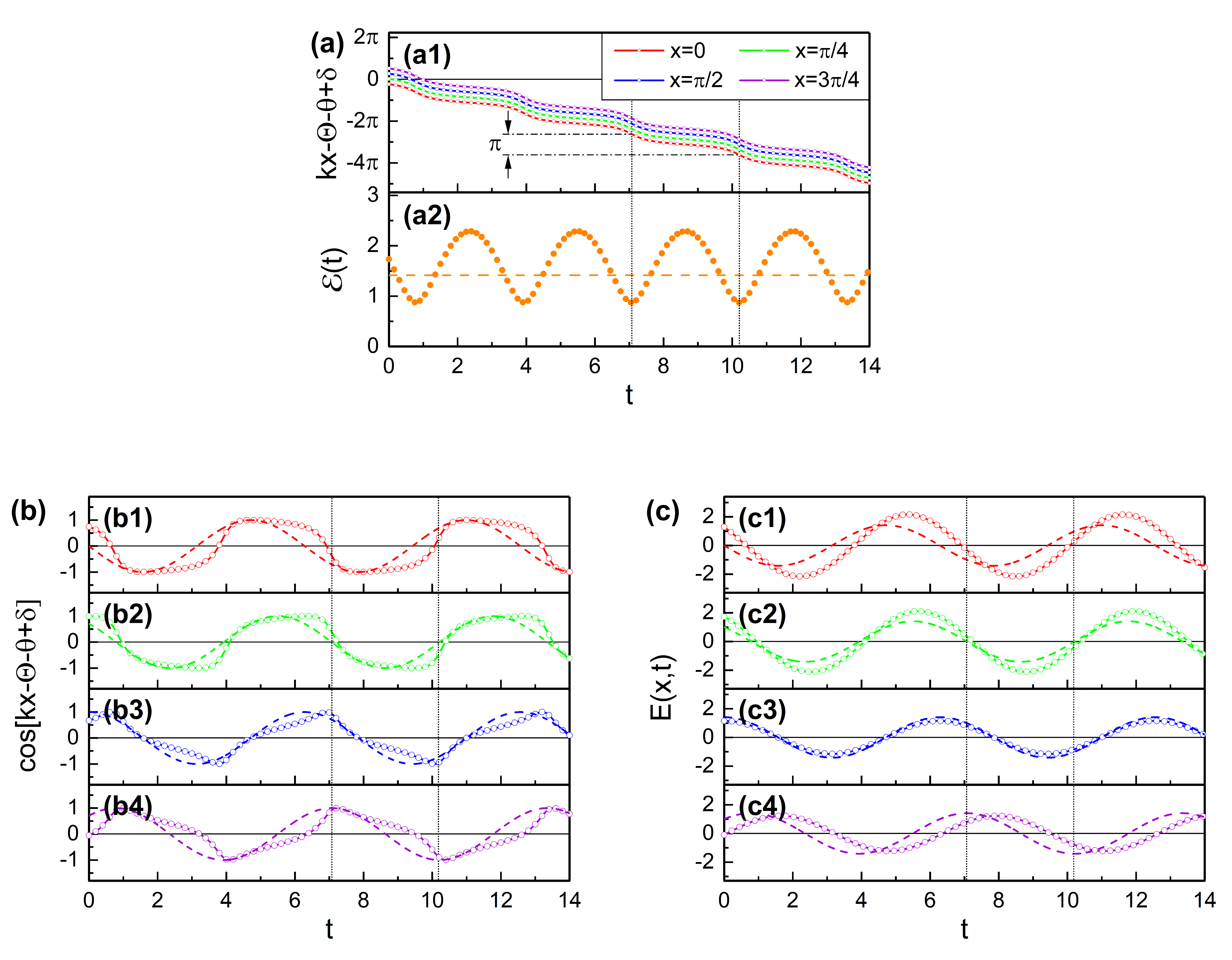
From Fig. 3, we can confirm the emergence of nonstaticity in the electric field as the measure of nonstaticity
deviates from zero.
Both the amplitude of E field and the phase factor deviate from the normal ones as the wave nonstaticity takes place.
Figures 3(a1) and 3(a2) show that the amplitude is smallest whenever the phase drops highly.
During the amplitude evolves from its smallest one to the next smallest one,
the phase drops .
Of course, the phase factor varies significantly when the variation of the phase is great.
However, the resultant electric field varies normally even if it deviates from the static one.
The variation of E field has been augmented
for Figs. 3(c1) and 3(c2) as the nonstaticity arose for instance,
whereas that for Figs. 3(c3) and 3(c4) has been quenched slightly.
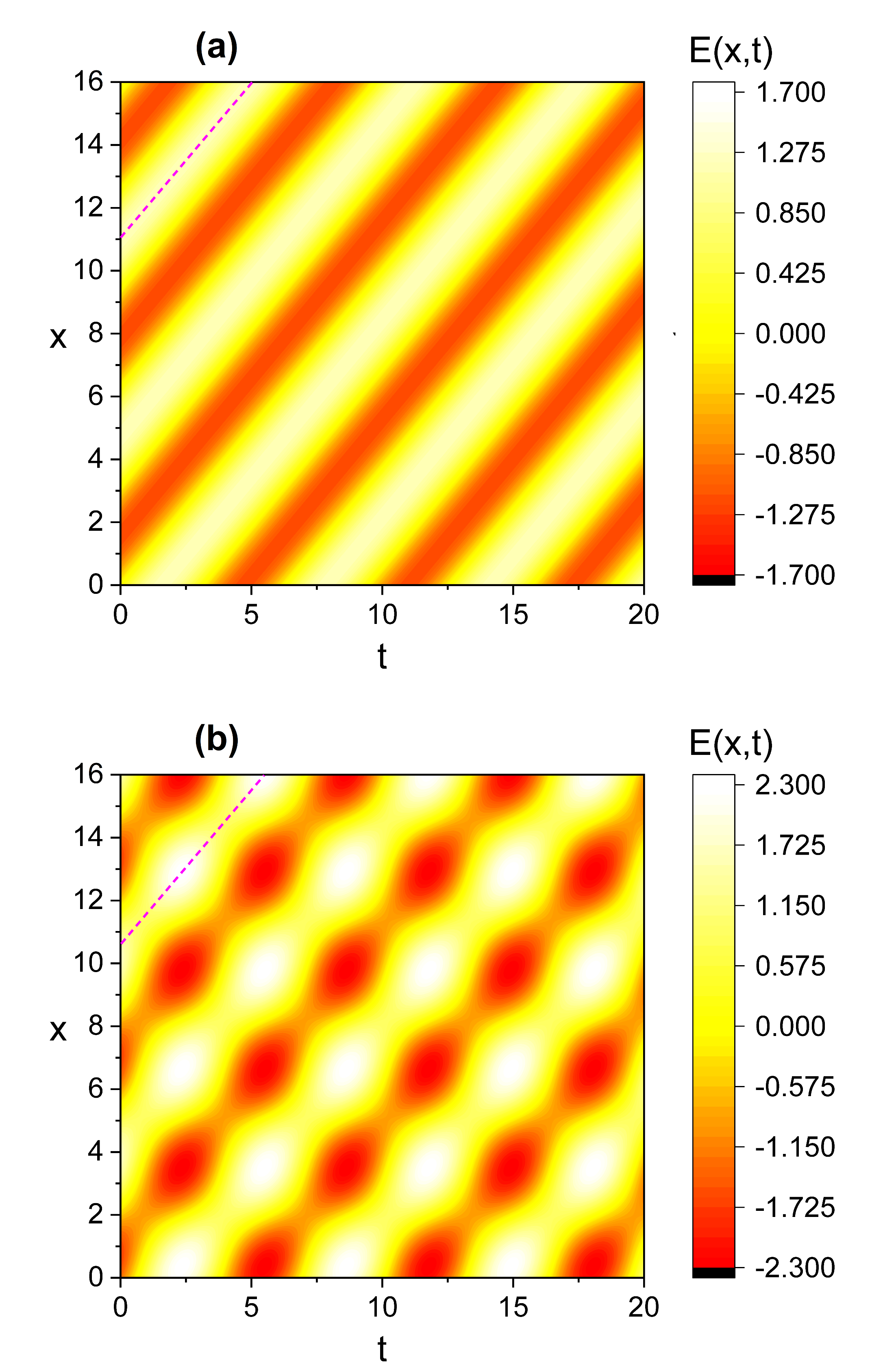
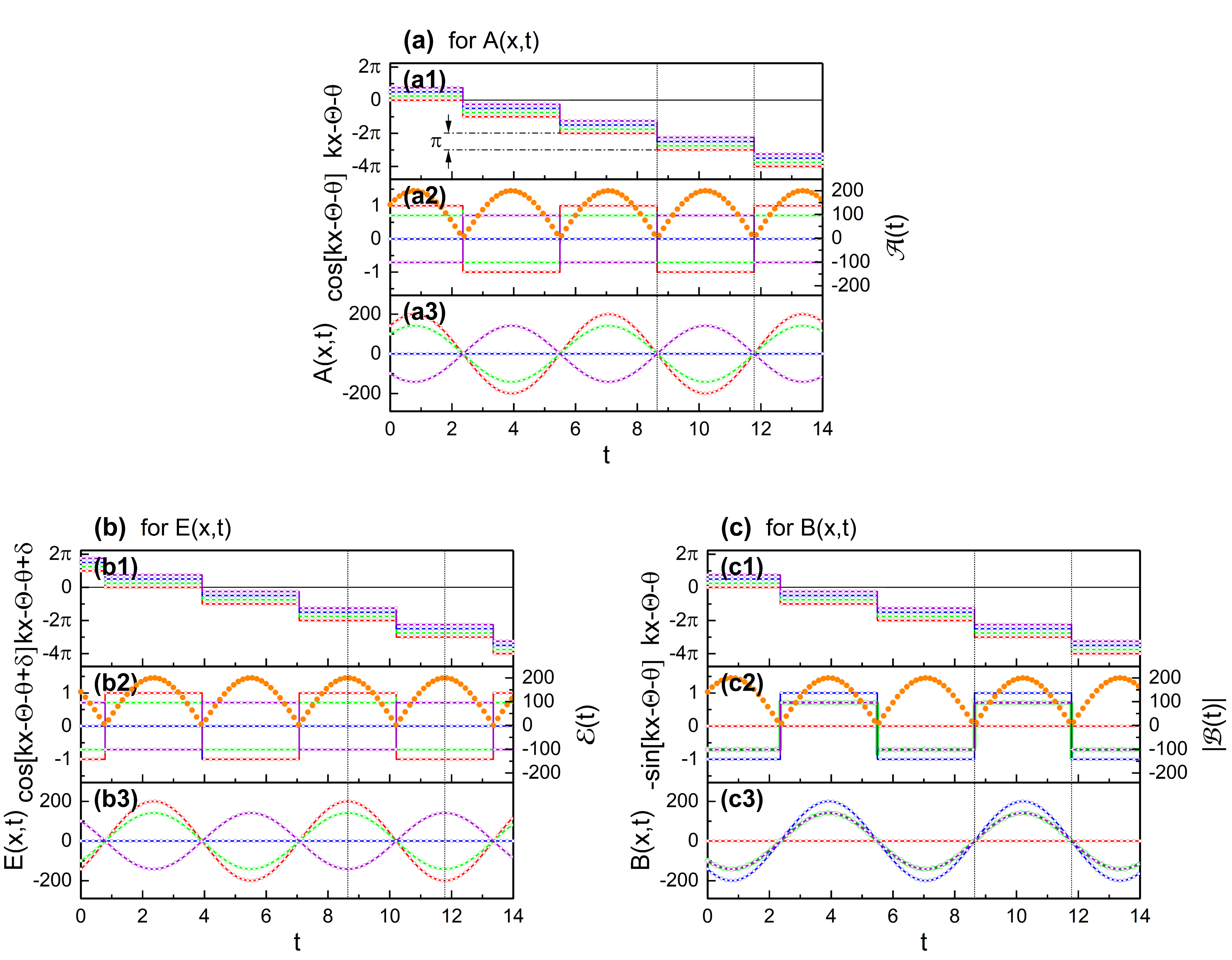
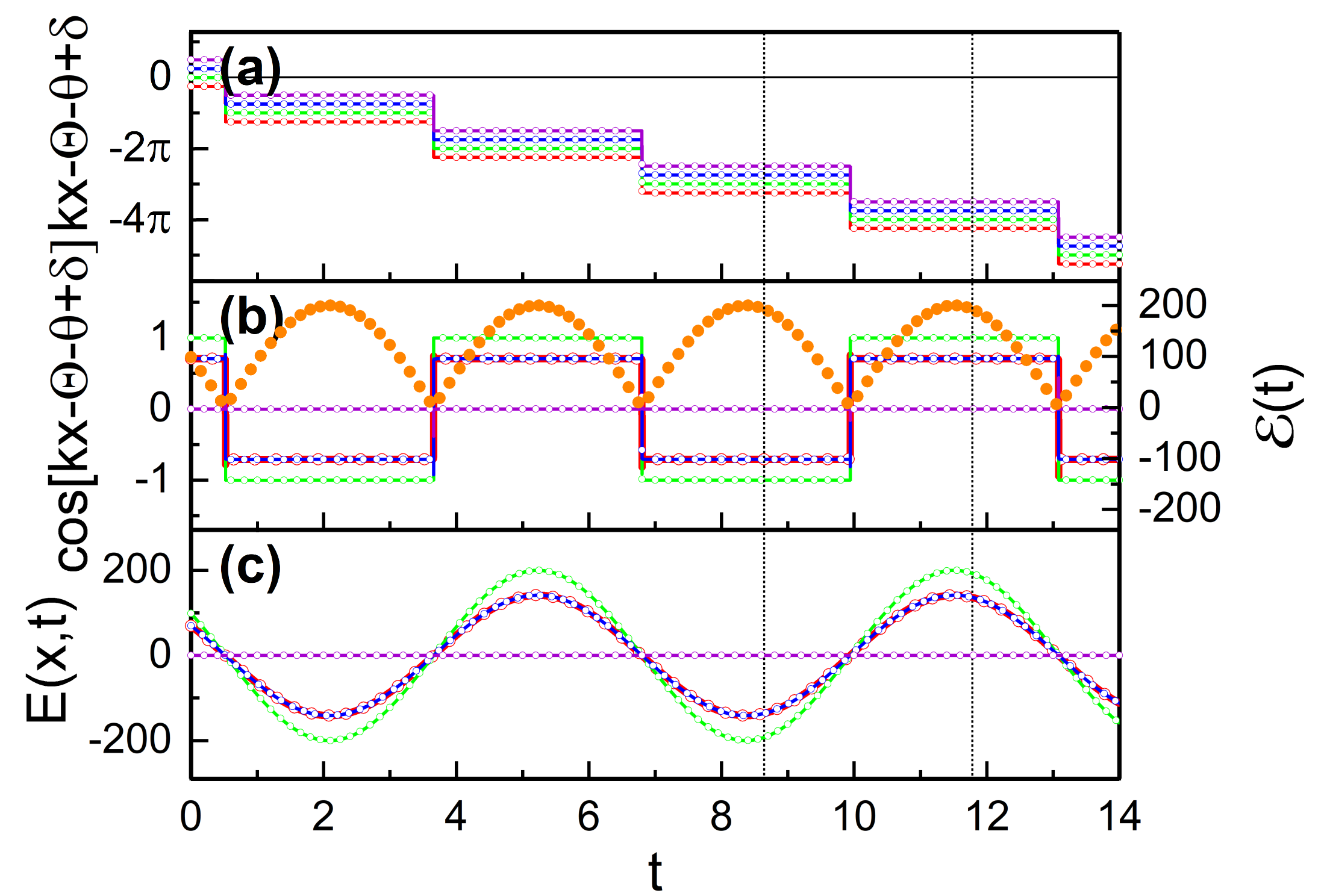
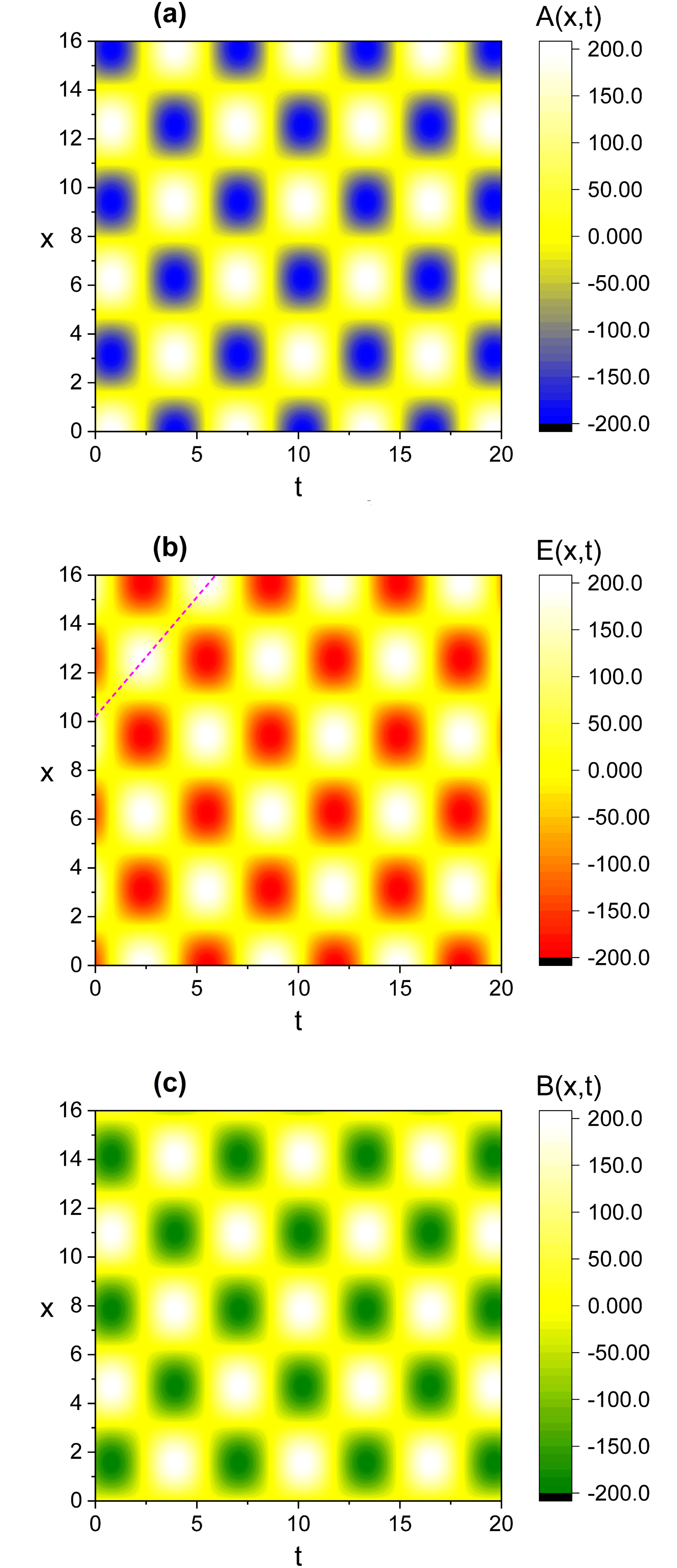
Figure 4 shows the spatiotemporal evolution of the electric field, where Fig. 4(a) is static and Fig. 4(b) is nonstatic ones.
From Fig. 4(b), you can confirm that the amplitude of the field is different depending on the position
as the wave becomes nonstatic.
The evolutions of the vector potential and the magnetic field for a nonstatic wave also exhibit
similar pattern as that of the nonstatic electric field.
From this discernible characteristic of nonstatic fields,
it is possible to distinguish the nonstatic electromagnetic wave from the ordinary wave experimentally.
Although we have seen only the case of electric field for brevity, the magnetic field also evolves in the same manner.
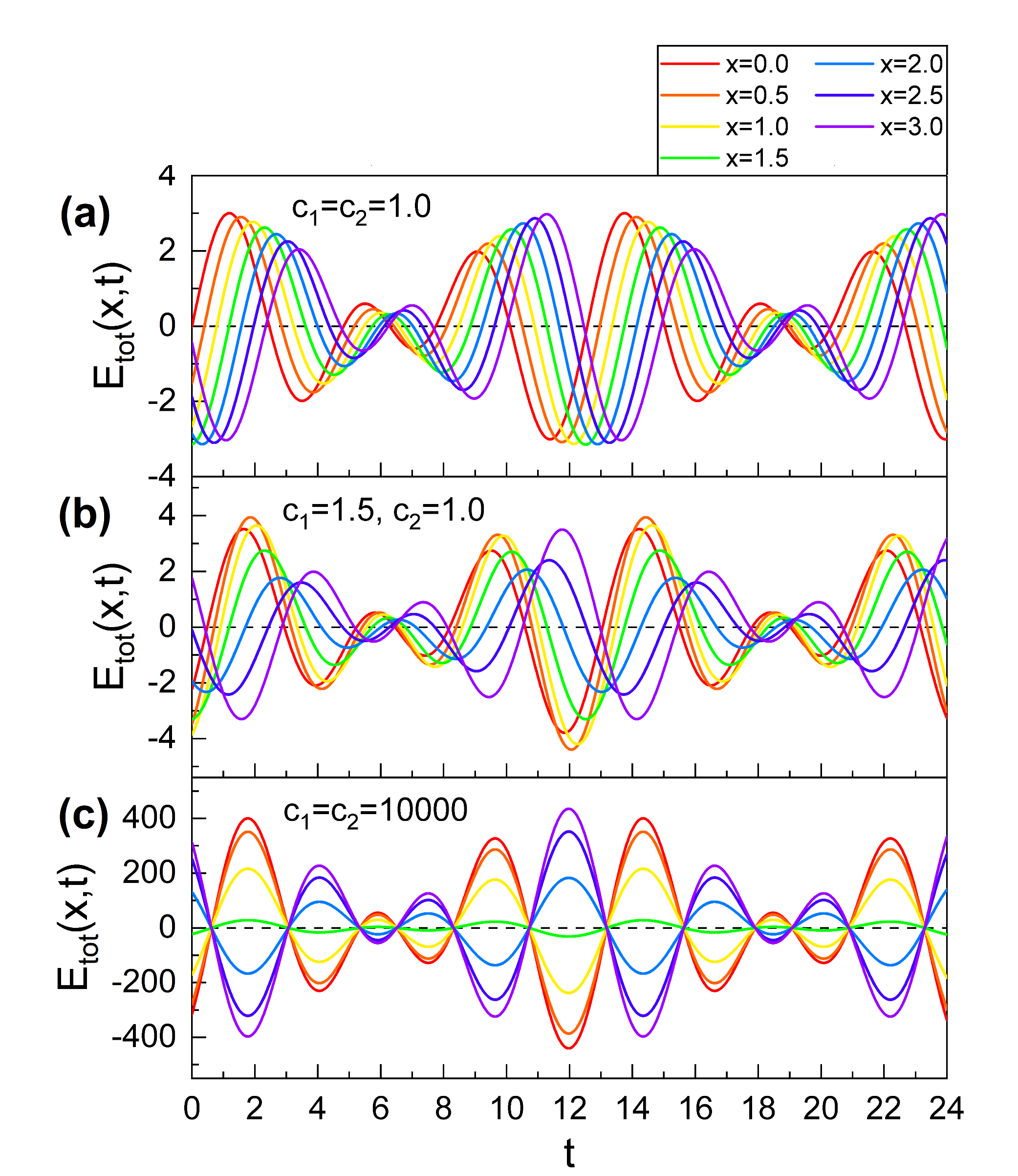
4.2. Evolution of extreme nonstatic electromagnetic waves
We now extend the wave evolution that we have examined in the previous subsection to
the extreme nonstatic case.
Figure 5 is the time evolution of several physical quantities related to
the vector potential and the electromagnetic
fields at equally-spaced four positions for an extreme nonstatic wave.
We see from this figure that the waves are quenched at some positions (for example, see the blue line
in Fig. 5(b3)), and active at other positions.
At a place where the waves are not completely quenched, the phase factor of a wave
evolves in a rectangular manner over time,
whereas the amplitude of the wave varies a lot.
Because the phase evolves during a period of amplitude variation,
the sign of phase factor changes whenever the phase drops: this is the reason for such rectangular
evolution of the phase factor.
However, the electric and magnetic fields take ordinary sinusoidal forms in their evolution.
This is due to the fact that not only the phase, but the amplitude of the wave also
varies in time. The time variation of the amplitude compensates the abnormal evolution of the
phase in a way that the resulting fields evolve sinusoidally.
If we only consider during a period of amplitude change,
it looks like that the roll of the amplitude and phase factor are changed each other.
Figure 5 together with Fig. 3 is useful for understanding the emergence of nonstaticity in electromagnetic waves. The variations of amplitudes shown in Fig. 3(a2) and Fig. 5(a2, b2, c2) themselves can be regarded as nonstaticity of waves in general. By comparing Fig. 5(b2) with Fig. 5(c2), the amplitude of B field is smallest (highest) whenever the amplitude of E field is highest (smallest). Such behaviors of the amplitudes are responsible for the variation of the quadratures uncertainties in the coherent state ncs . In more detail, the uncertainty of quadrature is great whenever is large, whereas the uncertainty of quadrature is great whenever is large.
We have seen the case where and from the graphical analyses of the evolution of the waves until now. However, even when and , the electromagnetic fields with a high nonstaticity also evolve with the same pattern given in Fig. 5. We can confirm this fact from Fig. 6 for the case of electric field for instance.
Figure 7 is the spatiotemporal evolution of , , and
for a highly nonstatic wave. In this case, the electric and magnetic fields are very similar to
those of the standing wave.
We almost do not know the propagation direction of the light wave based on only this figure.
In what follow, we can conclude that the wave propagates along positive direction.
For the cases of Figs. 4(a,b) and 7(b), the group velocity of the wave is the gradient of the
dashed line in the figures.
5. EFFECTS OF NONSTATICITY ON LIGHT-WAVE PHENOMENA
5.1. Superposition states
Based on the principle of superposition, a light wave is allowed to be in all possible states simultaneously
until it collapses to one of the basis states by its interaction with the
environment, or by a measuring of it.
Schrödinger’s cat is a good example of such superposed states.
In fact, quantum interference between element states of a superposed state
is responsible for various nonclassical effects such as sub-Poissonian
photon statistics, oscillation of photon number distribution, and higher-order squeezing nce1 ; nce2 .
The quantum phase of each substate plays a major role in the formation of
the overall probability distribution that accompanied such quantum interference
in a superposition state.
Let us consider a superposition of two Fock states, where the resultant wave function is of the form
| (18) |
The complex coefficients in this representation satisfy the normalization condition, which is . The corresponding probability density can be written as
| (19) |
where is the cross terms which lead to interference effects and is given by
| (20) |
The phase does not affect the first and second terms in the right-hand side of Eq. (19).
However, its effects in the third term (the cross terms) is non-negligible.
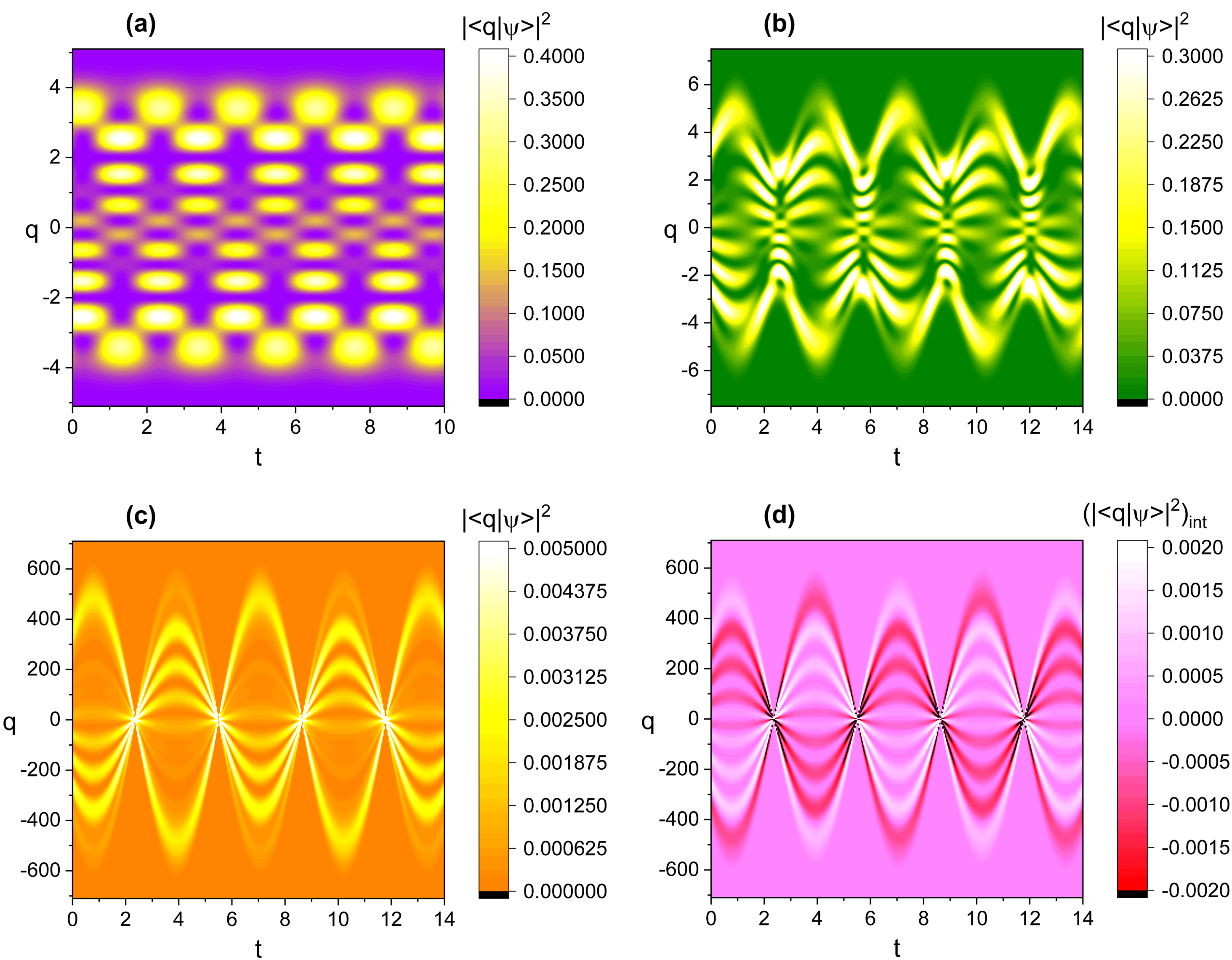
We have shown the evolution of in Fig. 8.
Figure 8(c) is a highly nonstatic case whereas Fig. 8(a) is the static case.
By comparing these two panels in Fig. 8, we confirm that the probability density in the extreme nonstatic case is
quite different from that of the ordinary superposed states.
Figure 8(c) exhibits that the original superposition pattern given in Fig. 8(a) is nearly annihilated by
the effect of the characteristic nonstaticity, whereas the variation of the wave amplitude is dominant instead.
We see from Fig. 8(d) that the interference term also exhibits a similar outcome.
5.2. Interference effects
As is well known, interference between light waves is an evidence of their wave-like property,
where the phase plays the key concept in its interpretation.
The physical effects of interference can be utilized to the development
of quantum information science and technologies related to
quantum computing, quantum metrology, and quantum communication tpi1 ; tpi2 ; tpi3 ; tpi4 .
When two or more nonstatic waves interact each other, the
geometric phase in each wave component may alter the interference pattern.
We consider interference of two nonstatic coherent waves whose frequencies are different from each other. Let us write the frequencies of the two waves as and , respectively. Then, the resultant electric field is expressed as
| (21) |
where
and
, while is
the one given in Eq. (16).
The magnetic field can also be represented in a similar manner.
The time evolution of the field in Eq. (21), where and ,
is illustrated in Fig. 9.
We can see beating
from each panel of this figure, which was produced on account of the difference in frequency
between the two component fields.
Although the beating for the static wave is even through each position, it
becomes gradually uneven as the measure of nonstaticity increases.
The mean amplitude of the beating electric field is different depending on the position for nonstatic waves.
For instance, for the case of Fig. 9(b), the amplitude
is highest at and smallest at among the considered seven positions.
For a highly nonstatic wave given in Fig. 9(c),
the electric field is relatively very weak at .
By the way, the phase difference between wave profiles whose positions are different
each other becomes negligible as the nonstaticity in the waves is being enhanced.
This is due to the fact that the nonstaticity is an effect associated with temporal variation of the wave,
but not related to its spatial variation.
However, the beating effect that happened due to such interference in the waves still remains
independently of the scale of nonstaticity.
6. CONCLUSION AND OUTLOOK
We have investigated the effects of wave nonstaticity for light propagating in a static environment focusing
on the situation where the measure of nonstaticity is high.
We have shown that, if the measure of nonstaticity is extremely high,
the phase of the wave function evolves in a periodic step-like manner, i.e., it drops vertically
whenever the wave constitutes a node in the quadrature space.
The effects of such a step phase on the superposed quantum states
and wave interference, as well as on the evolution
of the associated electromagnetic waves, have been investigated.
The time evolution of the nonstatic electromagnetic wave is abnormal due to the above-mentioned peculiar phase property in the wave functions. The evolution profile of the phase factor in the electromagnetic wave over time is a rectangular type in a highly nonstatic case. However, the electric and magnetic components in the wave always evolve following the sinusoidal form like those in an ordinary wave. For the case that the wave nonstaticity is quite high, the electromagnetic waves are very much the same as the standing wave where we can hardly know their propagation direction from their temporal behavior.
The novel abrupt drop of the phase of the wave function is originated from the enhancing of the time-varying geometric phase as the nonstaticity of the wave augments. We confirmed that the superposition state and the interference of the electromagnetic waves in the nonstatic regime are very different from those in the ordinary wave due to the effects of the uncommon temporal behavior of the phase. In a superposition state, the detailed original superposition pattern in the evolution of the associated probability density was gradually rubbed out as the nonstaticity grows and, instead, the variation of the wave’s amplitude that arose due to its nonstaticity was pronounced.
Effects of interference between two nonstatic electromagnetic waves which have different frequencies were analyzed subsequently. In the extreme nonstatic limit in this analysis, the phase difference in the resultant interfering electromagnetic wave between different positions is nearly not recognized from the temporal wave profile by the dominance of the nonstaticity-induced characteristic in that profile: this outcome is due to the fact that the wave nonstaticity treated here is a phenomenon associated entirely with time variation of waves, while it is irrelevant to their spatial variation.
This work may provide a deeper understanding for the phase phenomena of nonstatic electromagnetic
waves which should be considered in wave manipulation in this context, especially for the phase modulation.
In order to utilize the nonstatic waves as a main resource in optical science and technology,
the demonstration of their rich properties associated with,
for example, the global phase coherence and its evolution that we have clarified may be necessary.
On one hand, the consequences of this research provide a tool for
characterizing how
the nonstatic fields affect light-matter interactions spatio-temporarily, which is in particular
important in the domain of ultrashort timescales wst1 ; wst2 ; wst3 .
Appendix A Formula of Eigenfunctions
Appendix B Measure of Nonstaticity
Appendix C The Dynamical and the Geometric Phases
The analytical formulae of the dynamical phase and the geometric phase are given by gow
| (24) | |||||
| (25) |
References
- (1) J. R. Choi, On the possible emergence of nonstatic quantum waves in a static environment. Nonlinear Dyn. 103(3), 2783–2792 (2021).
- (2) J. R. Choi, Effects of light-wave nonstaticity on accompanying geometric-phase evolutions. Opt. Express 29(22), 35712–35724 (2021).
- (3) J. R. Choi, Analysis of light-wave nonstaticity in the coherent state. Sci. Rep. 11, 23974 (2021).
- (4) J. R. Choi, Geometric phase for a nonstatic coherent light-wave: Nonlinear evolution harmonized with the dynamical phase. arXiv:2401.12560v2 [quant-ph] (2024).
- (5) I. G. Koprinkov, Causality of phase of wave function or can Copenhagen interpretation of quantum mechanics be considered complete? J. Mod. Phys. 7(4), 390–394 (2016).
- (6) D. Richter, A. Magunia, M. Rebholz, C. Ott, and T. Pfeifer, Electronic population reconstruction from strong-field-modified absorption spectra with a convolutional neural network. Optics 5(1), 88–100 (2024).
- (7) A. J. Howard, M. Britton, Z. L. Streeter, C. Cheng, R. Forbes, J. L. Reynolds, F. Allum, G. A. McCracken, I. Gabalski, R. R. Lucchese, C. W. McCurdy, T. Weinacht, and P. H. Bucksbaum, Filming enhanced ionization in an ultrafast triatomic slingshot. Commun. Chem. 6, 81 (2023).
- (8) D. Chatterjee, Y. Bouasria, F. Goldfarb, and F. Bretenaker, Analytical seven-wave model for wave propagation in a degenerate dual-pump fiber phase sensitive amplifier. J. Opt. Soc. Am. B 38(4), 1112–1124 (2021).
- (9) T.-M. Nguyen, S. Song, B. Arnal, Z. Huang, M. O’Donnell, and R. K. Wang, Visualizing ultrasonically induced shear wave propagation using phase-sensitive optical coherence tomography for dynamic elastography. Opt. Lett. 39(4), 838–841 (2014).
- (10) P. Rocca, Q. J. Zhu, E. T. Bekele, S. W. Yang, and A. Massa, 4-D arrays as enabling technology for cognitive radio systems. IEEE Trans. Antennas Propag. 62(3), 1102–1116 (2014).
- (11) R. Maruyama, D. Yoshida, K. Nagano, K. Kuramitani, H. Tsurusawa, and T. Horikiri, Space-division multiplexed phase compensation for quantum communication: concept and field demonstration. arXiv:2401.15882v1 [quant-ph] (2024).
- (12) M. Taghinejad, H. Taghinejad, Z. Xu, K.-T. Lee, S. P. Rodrigues, J. Yan, A. Adibi, T. Lian, and W. Cai, Ultrafast control of phase and polarization of light expedited by hot-electron transfer. Nano Lett. 18(9), 5544–5551 (2018).
- (13) Y. Luan, T. Yang, J. Ren, R. Li, and Z. Zhang, Broadband beam-scanning phased array based on microwave photonics. Electronics 13(7), 1278 (2024).
- (14) B. O. Zhu, K. Chen, N. Jia, L. Sun, J. Zhao, T. Jiang, and Y. Feng, Dynamic control of electromagnetic wave propagation with the equivalent principle inspired tunable metasurface. Sci. Rep. 4, 4971 (2014).
- (15) M. Secmen, S. Demir, A. Hizal, and T. Eker, Frequency diverse array antenna with periodic time modulated pattern in range and angle. in Proc. of 2007 IEEE Radar Conference (IEEE, Boston, MA, USA, 2007), pp. 427–430.
- (16) Y. Yao, R. Shankar, M. A. Kats, Y. Song, J. Kong, M. Loncar, and F. Capasso, Electrically tunable metasurface perfect absorbers for ultrathin mid-infrared optical modulators. Nano Lett. 14(11), 6526–6532 (2014).
- (17) K. Chen, Y. Feng, F. Monticone, J. Zhao, B. Zhu, T. Jiang, L. Zhang, Y. Kim, X. Ding, S. Zhang, A. Alù, and C.-W. Qiu, A reconfigurable active Huygens’ metalens. Adv. Mater. 29(17), 1606422 (2017).
- (18) T. Remetter, P. Johnsson, J. Mauritsson, K. Varjú, Y. Ni, F. Lépine, E. Gustafsson, M. Kling, J. Khan, R. López-Martens, K. J. Schafer, M. J. J. Vrakking, and A. L’Huillier, Attosecond electron wave packet interferometry. Nat. Phys. 2, 323–326 (2006).
- (19) E. O. Kamenetskii, R. Joffe, and R. Shavit, Coupled states of electromagnetic fields with magnetic-dipolar-mode vortices: Magnetic-dipolar-mode vortex polaritons. Phys. Rev. A 84(2), 023836 (2011).
- (20) T. Dumelow, R. E. Camley, K. Abraha, and D. R. Tilley, Nonreciprocal phase behavior in reflection of electromagnetic waves from magnetic materials. Phys. Rev. B 58(2), 897–908 (1998).
- (21) L. Kolokolova, E. Petrova, and H. Kimura, Effects of interaction of electromagnetic waves in complex particles. in Electromagnetic Waves (Intech Open, Rijeka, 2011).
- (22) J. P. Dowling and G. J. Milburn, Quantum technology: the second quantum revolution. Philos. Trans. A: Math. Phys. Eng. Sci. 361(1809), 1655–1674 (2003).
- (23) N. F. Costa, Y. Omar, A. Sultanov, and G. S. Paraoanu, Benchmarking machine learning algorithms for adaptive quantum phase estimation with noisy intermediate-scale quantum sensors. EPJ Quantum Technol. 8(1), 16 (2021).
- (24) E. Strambini et al., A Josephson phase battery. Nat. Nanotechnol. 15(8), 656–660 (2020).
- (25) V. Vedral, Geometric phase and topological quantum computation. Int. J. Quantum Inf. 1(1), 1–23 (2003).
- (26) H. Zhou, R. Douvenot, and A. Chabory, Modeling the long-range wave propagation by a split-step wavelet method. J. Comput. Phys. 402, 109042 (2020).
- (27) Q. Zhan, Spatiotemporal sculpturing of light: a tutorial. Adv. Opt. Photon. 16(2) 163–228 (2024).
- (28) W. H. Louisell, Quantum Statistical Properties of Radiation (John Wiley and Sons, New York, 1973), Chapters 4.3. and 4.4.
- (29) M. S. Kim and V. Buz̆ek, Photon statistics of superposition states in phase-sensitive reservoirs. Phys. Rev. A 47(1), 610–619 (1993).
- (30) T. A. B. Kennedy and D. F. Walls, Squeezed quantum fluctuations and macroscopic quantum coherence. Phys. Rev. A 37(1), 152–157 (1988).
- (31) H. Kim, O. Kwon, and H. S. Moon, Two-photon interferences of weak coherent lights. Sci. Rep. 11, 20555 (2021).
- (32) Z. S. Yuan, X.-H. Bao, C.-Y. Lu, J. Zhang, C.-Z. Peng, and J.-W. Pan, Entangled photons and quantum communication. Phys. Rep. 497(1), 1–40 (2010).
- (33) A. Y. Shiekh, The role of quantum interference in quantum computing. Int. J. Theor. Phys. 45(9), 1646–1648 (2006).
- (34) Z.-E. Su, Y. Li, P. P. Rohde, H.-L. Huang, X.-L. Wang, L. Li, N.-L. Liu, J. P. Dowling, C.-Y. Lu, and J.-W. Pan, Multiphoton interference in quantum Fourier transform circuits and applications to quantum metrology. Phys. Rev. Lett. 119(8), 080502 (2017).
- (35) X. Zhang, F. Wang, Z. Liu, X. Feng, and S. Pang, Controlling energy transfer from intense ultrashort light pulse to crystals: A comparison study in attosecond and femtosecond regimes. Phys. Lett. A 384(27), 126710 (2020).
- (36) H. Wang, S. M. Meyer, C. J. Murphy, Y.-S. Chen, and Y. Zhao, Visualizing ultrafast photothermal dynamics with decoupled optical force nanoscopy. Nature Commun. 14, 7267 (2023).
- (37) R. Gutzler, M. Garg, C. R. Ast, K. Kuhnke, and K. Kern, Light-matter interaction at atomic scales. Nat. Rev. Phys. 3, 441–453 (2021).