Exponential Modification of AdS Black Hole and Thermodynamic Behavior
Mehdi Sadeghi and Faramaz Rahmani
Department of Physics, Faculty of Basic Sciences,
Ayatollah Boroujerdi University, Boroujerd, IranCorresponding author: Email: mehdi.sadeghi@abru.ac.irEmail: faramarz.rahmani@abru.ac.ir
Abstract
In this paper, we present an exponential modification for the action of an AdS black hole in the absence of a matter field. An approximated black hole solution is obtained up to the third order of perturbation coefficient. A thermodynamic investigation in canonical ensemble shows that the behavior of a Van der Waals fluid is not seen in this model. Nevertheless, the study of thermodynamic potentials and other related quantities suggests that the thermodynamic phase transitions of the first and second types can occur in this model. The forms of the phase transitions are more similar to the Hawking-Page phase transitions.
PACS numbers: 04.50.Kd, 97.60.Lf
Keywords: Modified gravity, Black hole
1 Introduction
Einstein’s theory of general relativity has been one of the most successful theories of physics so far. Before this theory, the nature of gravity was not obvious to anyone. But with Einstein’s clever idea, which originated from the principle of equivalence, gravity was introduced as the curvature of spacetime, and experimental observations after that confirmed the correctness of this theory. One of the challenging issues has been the issue of unifying gravity and quantum mechanics. So far, such an approach suffers from several problems such as renormalization of the theory or the presence of ghosts in the solutions of the theory. It is expected that the modification of gravitational actions with higher order terms helps us to create a quantum theory of gravity. Therefore, during the last few decades, many efforts have been made in this field. Nevertheless, general relativity (GR), which was formulated by Albert Einstein in 1915, has achieved significant milestones such as gravitational waves, the Mercury anomaly, gravitational lensing, and black holes. Observational data confirm that 95 of the Universe consists of dark energy (about 69) and dark matter (about 26), which are unknown. GR has failed to account for this unidentified portion of the Universe. Additionally, General Relativity’s non-renormalizability has impeded its quantization using conventional methods in quantum field theory. Therefore, modifications were made to GR to address these limitations, including the incorporation of Dark Energy and Dark Matter, and the unification of Gravity with quantum mechanics[1]. gravity[2],[3][4], Lovelock gravity[5], Gauss-Bonnet gravity[6][7], Quasi-topological gravity[8], massive gravity[9],[10],[11] the Rastall theory of gravity[12],[13] and exponential modified gravity[14][15][16][17] are some of the modifications of general relativity found in the literature.
One of the places where quantum and gravitational concepts can intertwine and make us understand more relevant concepts is where the thermodynamics of black holes are investigated. As we know, black holes have thermodynamic properties as solutions to the theory of general relativity. Black hole radiation (Hawking radiation) is a quantum phenomenon, and where gravity is very strong, a quantum gravity theory is required to properly understand the physics of this phenomenon. Therefore, the thermodynamic study of the black hole can be of great importance. Specifically, the study of phase transition in black holes provides insights into the fundamental properties of black holes and enables us to explore their thermodynamic stability. The thermodynamic behavior of black holes can be translated by using the AdS/CFT dictionary to study some fundamental issues like confinement-deconfinement phase transition or the problem of superconductivity which are investigated in the context of a conformal quantum field theory[18][19][20]. Phase transitions in black holes may open a way toward a quantum theory of gravity. They offer a playground for testing theories that attempt to unify general relativity and quantum mechanics, such as string theory and loop quantum gravity. The investigation of black hole thermodynamics and their phase transitions helps us to realize the quantum nature and fundamental laws governing black holes. In summary, phase transitions in black hole thermodynamics can provide profound insights into the nature of black holes, the structure of spacetime and the fundamental laws of physics.
In section (2), we introduce the exponential modification of the AdS black hole. Then, we obtain an approximated black hole solution up to the third order of perturbation coefficient. Finally, in section (3), the thermodynamic behavior of the model shall be studied in canonical ensemble to determine the types of phase transitions and stability of the system.
2 Exponential Modification of the AdS Black Hole
The 4-dimensional action of exponentially modified gravity with negative cosmological constant is [14],
(1)
where is the Ricci scalar, is the cosmological constant and is the AdS radius. When , the exponential term gets transformed into standard Einstein-Hilbert gravity.
The equations of motion are obtained by varying action (1) with respect to . This leads to equation
(2)
Our goal is to find an asymptotically AdS black hole solution of the above equation in four-dimensional maximally symmetric spacetime. In this regard, we consider the following ansatz,
(3)
Where is the metric function that shall be determined.
By using ansatz (3) and relation (2), the component of Eq. (2) gives
(4)
An exact solution for cannot be obtained. So, we consider a perturbed form for up to the third order of as bellow,
(5)
By substituting the relation (5) into equation (4) and considering the coefficient of the zeroth order of , the following equation is obtained as bellow,
(6)
The function is easily obtained through the solving of the above equation. The result is
(7)
Where, is an integration constant related to the mass of the black hole.
Up to the second order of in Eq.(4), the related coefficient gives an equation as follows,
(12)
By solving this equation, is given by
(13)
As the same way, is obtained as follows,
(14)
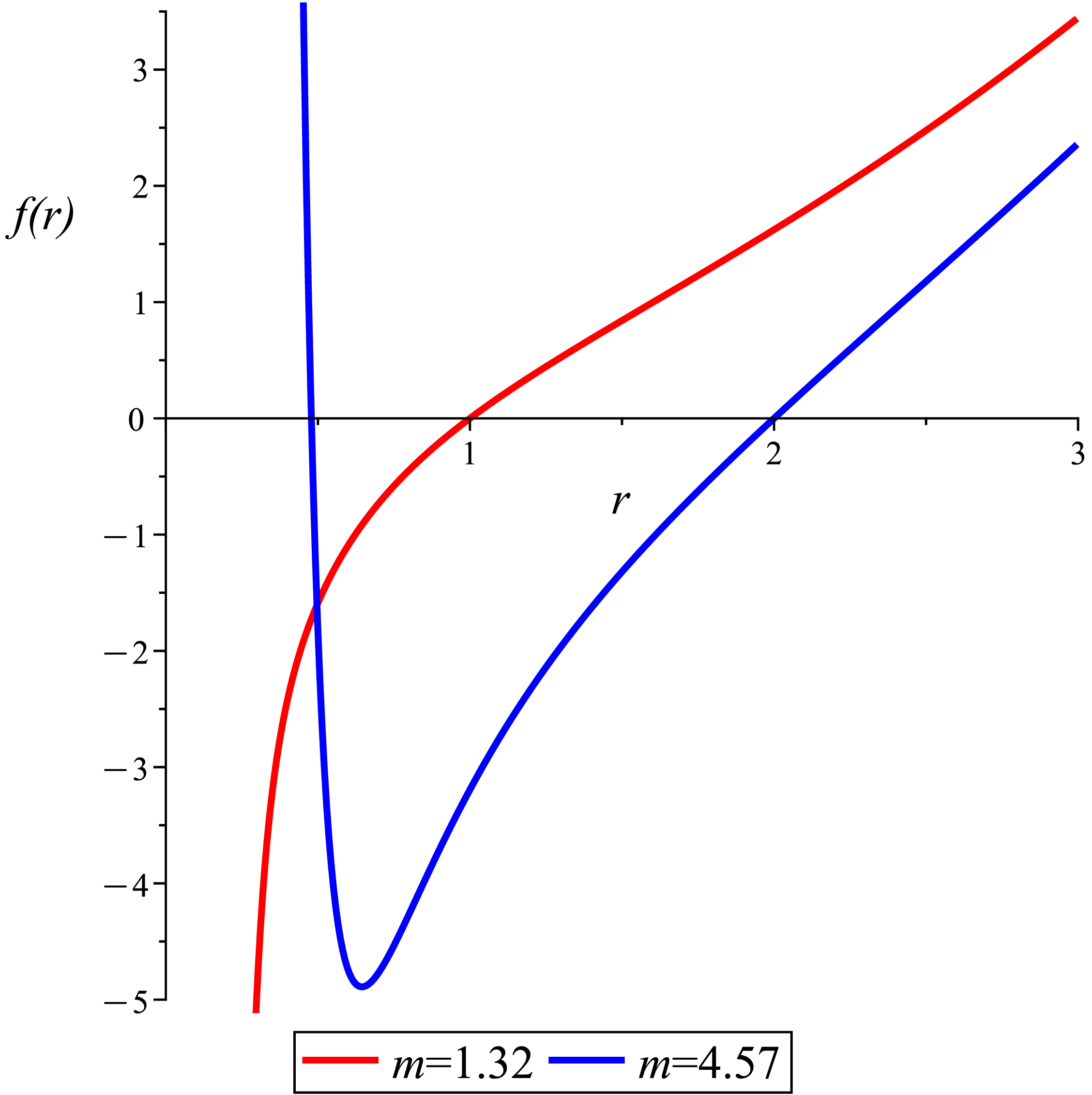
[a] [b]
Figure 1: diagrams when (a): , ; (b): and outer horizon is at . In the left panel the value of the is fixed and by increasing the value of , the number of roots increases. In the right panel the value of changes.
Since, each of the functions and vanish on the horizon of the black hole, the unknown coefficients and can be determined easily. The numerator of the term , in metric functions is proportional to the integration constant . With this consideration, the ADM mass is obtained in terms of powers of which up to the second order of is expressed as bellow,
(15)
where,
(16)
(17)
and
(18)
The behavior of for various values of parameters is seen in Fig. (1). Investigations show that for different values of parameters, the function has at most two roots in this model.
Now, the Hawking temperature[21] for this black hole solution up to the second order of is
(19)
One can see that when , the mass and temperature of this model are the same as the mass and temperature of the Schwarzchild-AdS black hole.
The entropy of our model is calculated using the Wald formula [22] as follows,
(20)
where,
(21)
Furthermore,
(22)
(23)
and
(24)
Calculations give the following relation for the Ricci scalar,
Where after substituting relation (26) into relation (27), we get
(28)
where,
(29)
(30)
(31)
(32)
and
(33)
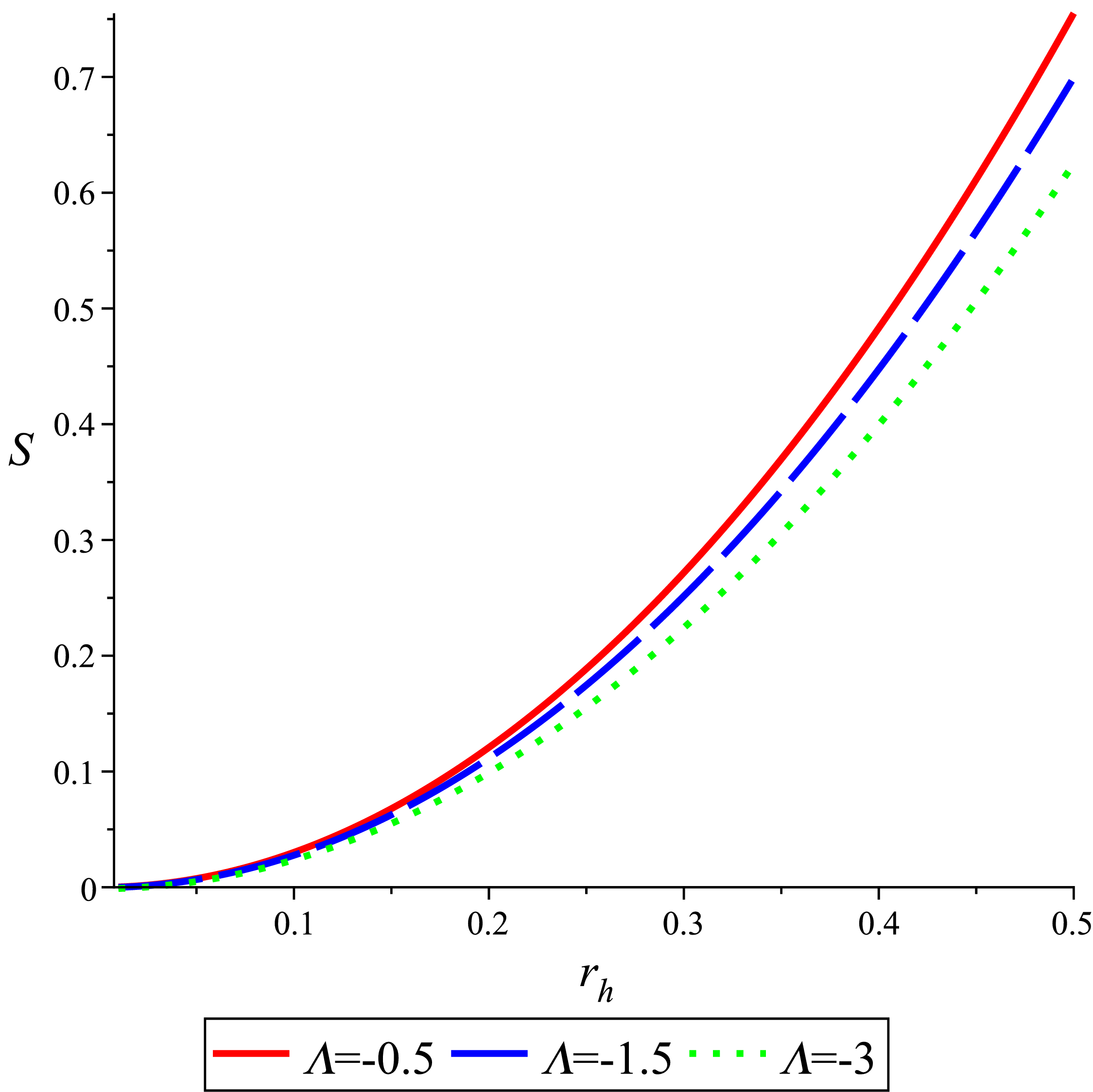
[a] [b]
Figure 2: The diagrams of entropy versus the black hole horizon for several values of and ; (a): up to the third order of and (b): up to the fourth order of . In the right panel, for small values of the black hole horizon, the entropy of the system increases.
As we expect, by increasing the horizon of the black hole, the entropy of the system increases and vice versa. This is obvious from the left panel of Fig.(2) which shows the entropy diagram up to the third order of . But, in the right panel which shows the entropy up to the fourth order of , a minimum for each diagram is seen and for small horizons, the entropy of the system increases. This is not a classical phenomenon and may be a sign of quantum effects.
3 Thermodynamic Stability and Phase Transitions
Usually, in the study of thermodynamic behavior of black hole solutions in extended phase space, we need to obtain the mass of the black hole which plays the role of enthalpy of the system. For a four-dimensional AdS black hole, the enthalpy is equal to the integration constant which appears in the numerator of the term in the metric function. Here, stands for the dimension of spacetime. The general relation between the enthalphy (mass) of the black hole and integration constant is as follows[23],
(34)
where, is the volume of the -dimensional unit sphere and is determined through the relation
(35)
In -dimensional models, the enthalpy of the system is equal to the integration constant . Hence, by using the relations (16), (17) and (18) and [23], the enthalpy of the system is given by
(36)
The conjugate volume for the system pressure is given by
(37)
When , the conjugate volume is equal to the usual volume of a simple Schwarzschild-AdS black hole.
The pressure of this model up to the second order of is given by,
(38)
To have a correct Smarr formula, the coupling constant should be considered as a charge with a potential as follows,
(39)
Now, the first law of thermodynamics takes the form
(40)
The Smarr formula reads as111First, a general Smarr formula was considered in the form . Then, through an examination we realized that the value ensures a correct Smarr formula up to the first order of .
(41)
up to the linear order in .
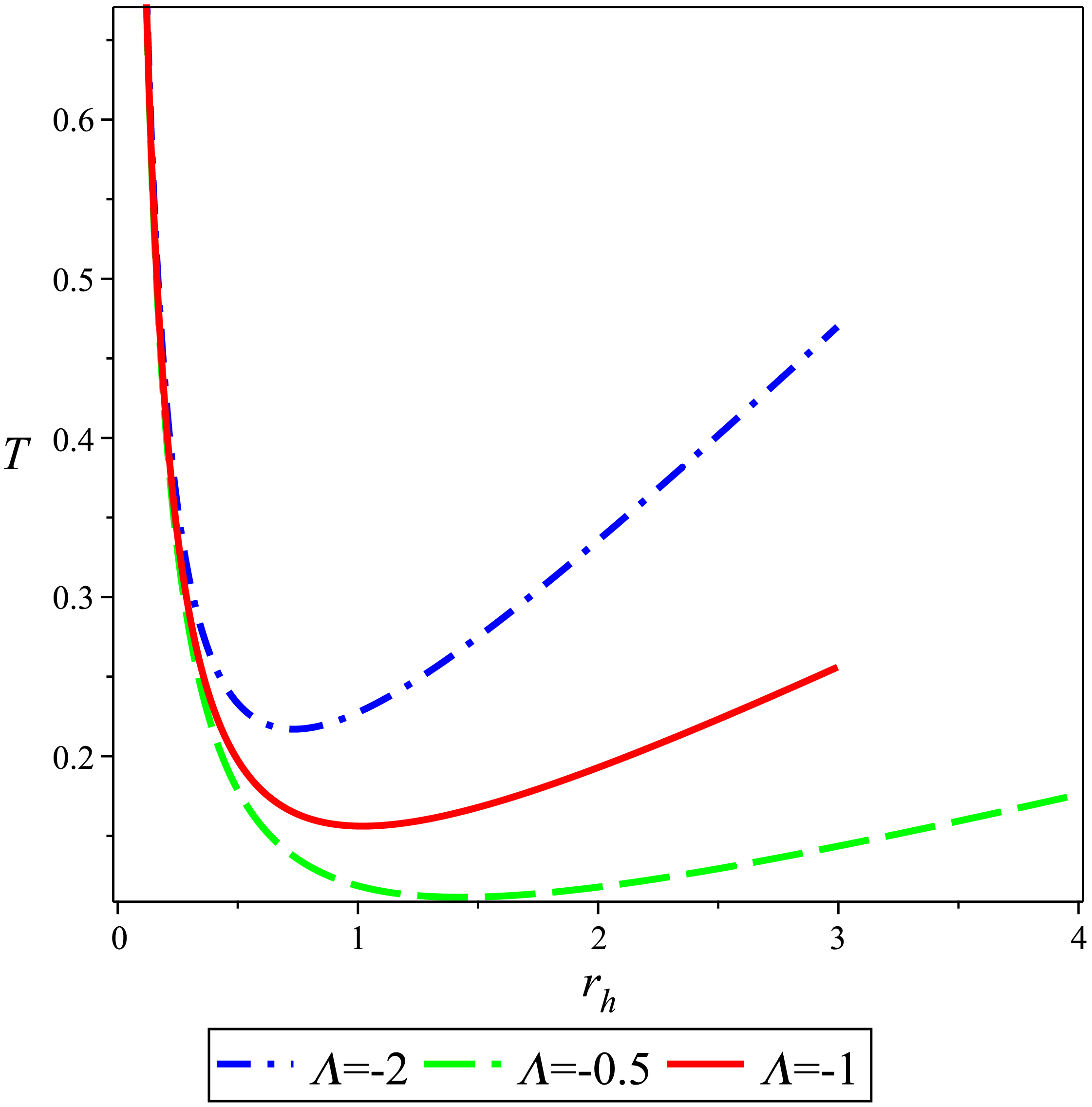
Investigations show that the pressure and temperature diagrams of this model do not correspond to the pressure and temperature diagrams of a Van der Waals fluid. Fig. (3) shows that for different values of parameters, the temperature of the system has a minimum value. The minimum of the temperature when has expressed up to the first and second order of occurs at horizons
(42)
and
(43)
respectively. Below these temperatures, no black hole can exist. This is what happens in the Hawking-Page transition. For temperatures higher than minimum temperature, two branches are seen. By substituiting the relation (42) or (43) into the Hawking temperature of the system, the minimum temperature value can be estimated. For small horizons, the system is unstable, while for large horizons it is stable. Figure (3) shows the behavior of temperature against the black hole horizon for different values of the involved quantities. As increases, the minimum temperature moves upwards.
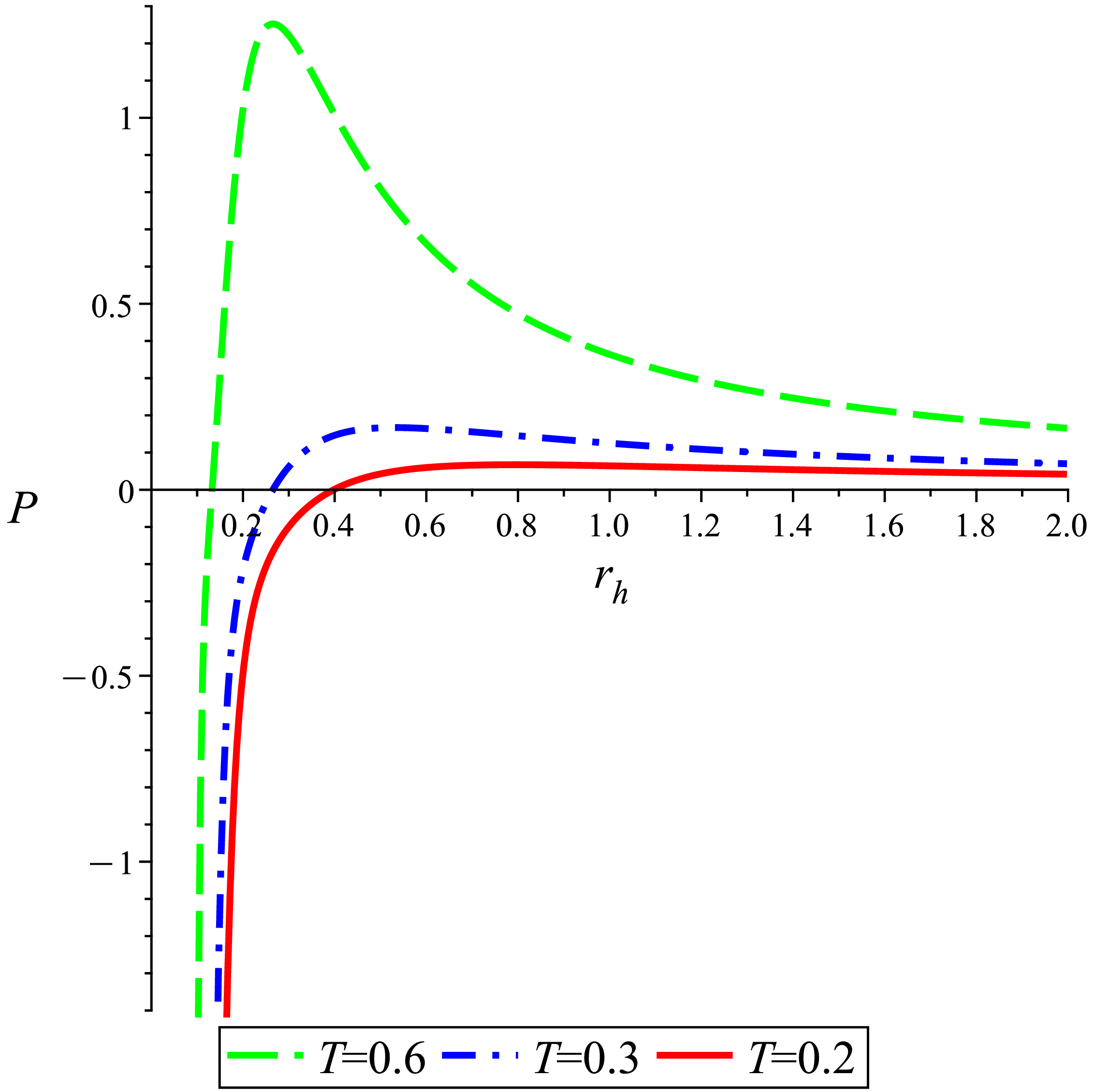
The behavior of the pressure against the horizon for different values of temperature and parameter is seen in Fig. (4). Van der Waal’s behavior is not seen in these diagrams. In other words, the conditions
or
are not satisfied in this model.
[a] [b]
Figure 3: diagrams up to the second order of when (a): the parameter changes and (b): the parameter changes. In both panels, minimum values are seen for the system temperature. Bellow the minimum values no black hole can exist. Above the minimum value two unstable and stable phases are seen.
[a] [b]
Figure 4: diagrams up to the second order of when (a): the temperature of the system changes and (b): the parameter changes. .
Nevertheless, there is a possibility of observing the first and second types of phase transitions in this model. For this purpose, we study the behavior of thermodynamic potentials like entropy and Gibbs free energy to see the signs of the first order phase transition. In order to see the signs of a second order phase transition, the functions like the heat capacity or isothermal compressibility of the system, which are proportional to the second derivative of the Gibbs function, are studied. Before that, let us see the behavior of the entropy versus the system temperature.
[a] [b]
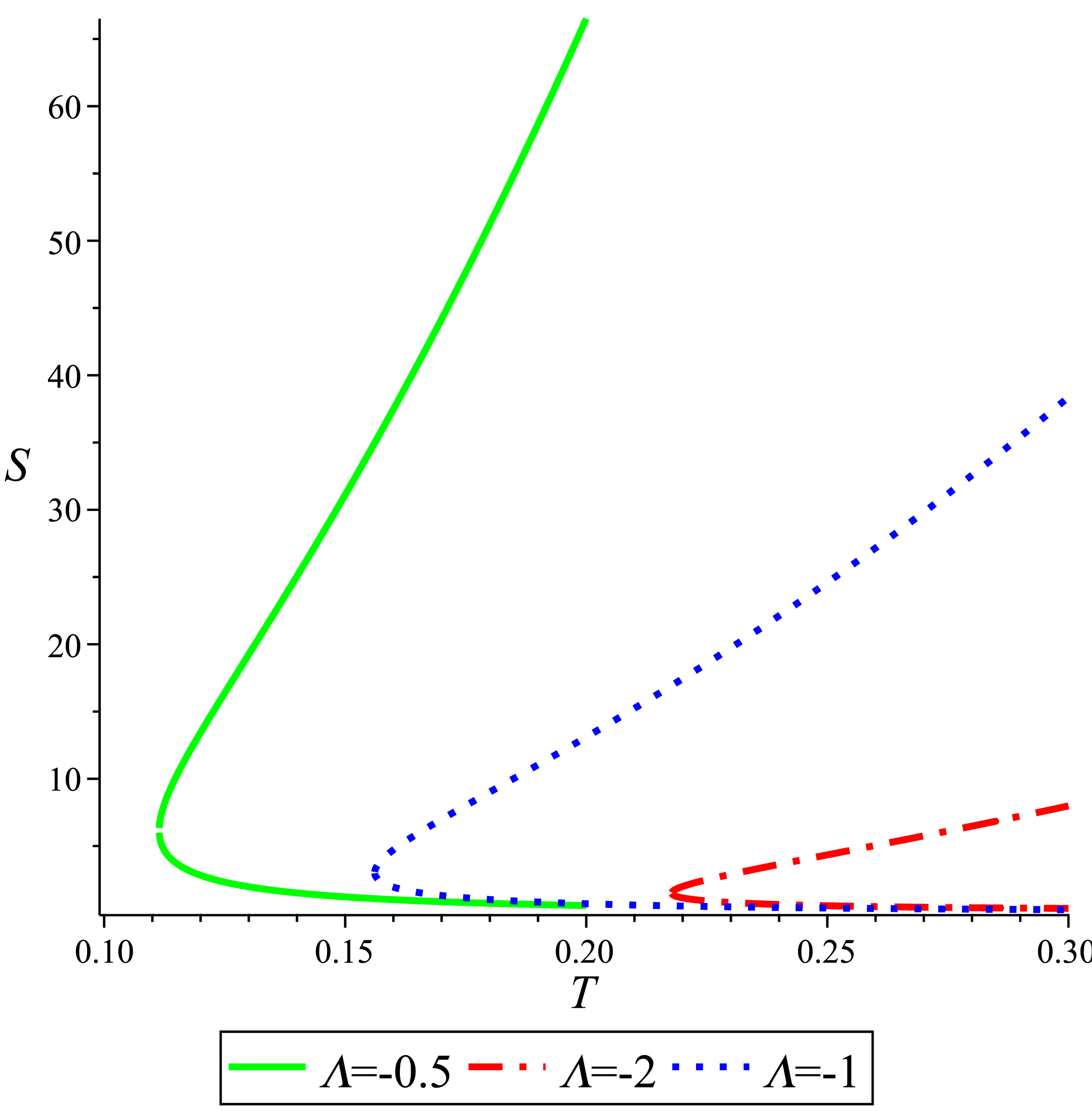
Figure 5: The diagrams of entropy versus temperature when (a): the value of changes, (b): the value of changes. A sudden change in the diagrams at a certain point can refer to a phase transition between unstable and stable black holes.
Fig. (5) shows the behavior of entropy against the temperature of the system. Phase transitions occur at critical points where the entropy or temperature exhibits sudden changes. The figure shows a transition between large and small black holes. By examining the entropy for several values of parameters and , we realized that this is not a stable system in general. The only difference in the diagrams is that the minimum value of the temperature at which the phase transition occurs is shifted to different values of the parameters. This is well illustrated in Fig. (5). The slope of the diagrams changes abruptly, indicating a phase transition.
Now, the Gibbs free energy of this model, which can give us more detailed information about the type of phase transition, is studied. The Gibbs free energy in terms of the black hole horizon has the following form:
(44)
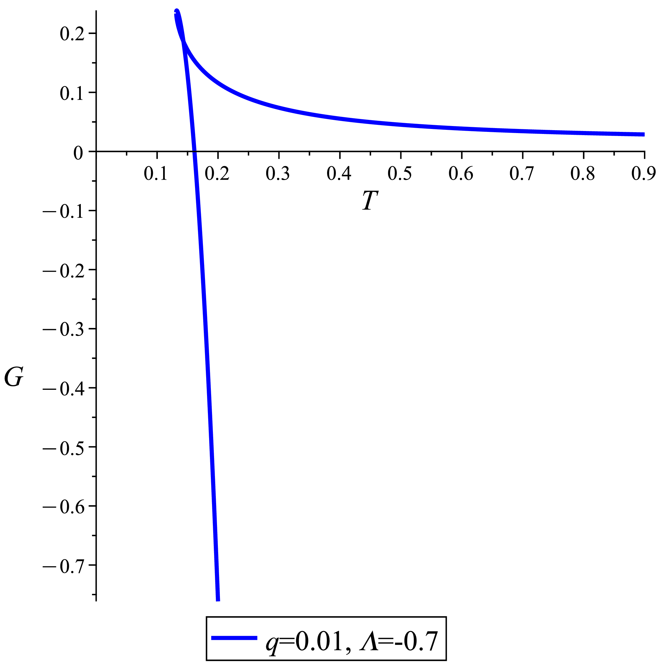
By using the relations (19) and (44) one can obtain a relation for the Gibbs free energy in terms of (or the pressure ) and the temperature of the black hole. The investigation of the Gibbs function versus temperature for different values of and expansion coefficient , leads to the diagrams of Fig. (6).
[a] [b] [c] [d]
Figure 6: diagrams for the different values of and ; (a): , (b): , (c): and (d): . The swallow-tail shapes of these diagrams and their behavior are similar to the Gibbs free energy diagrams of the Hawking-Page transition which indicate a first-order phase transition between small and large black holes.
In these diagrams, the swallow-tail shapes appear, but they are not exactly like the swallow-tail shapes of a Van der Waals fluid. Nevertheless, these diagrams confirm a first-order phase transition. These diagrams are more similar to the Hawking-Page phase transition diagrams. Where the Gibbs free energy diagrams intersect the horizontal axis(), it defines the Hawking-Page temperature in this model.
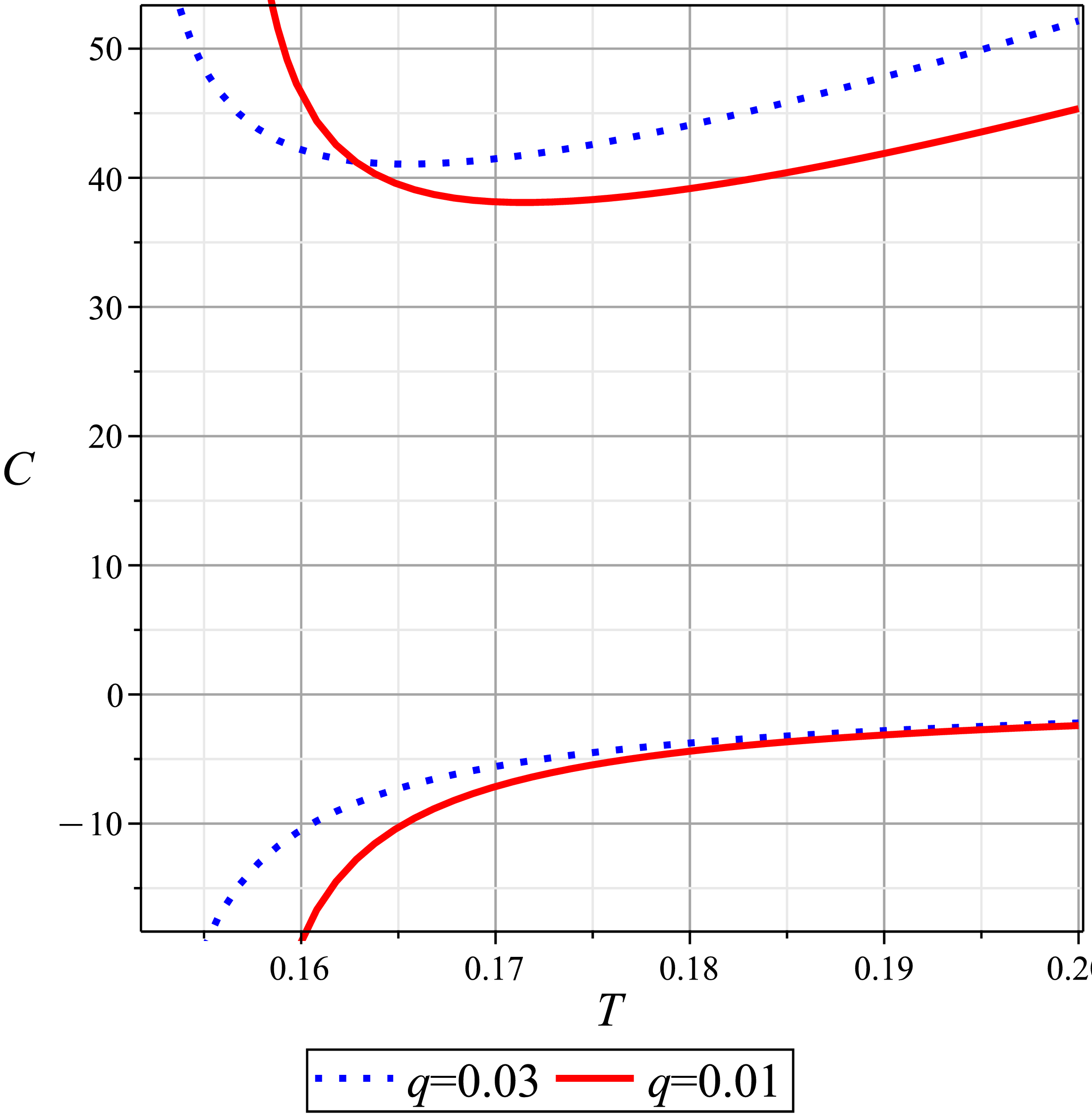
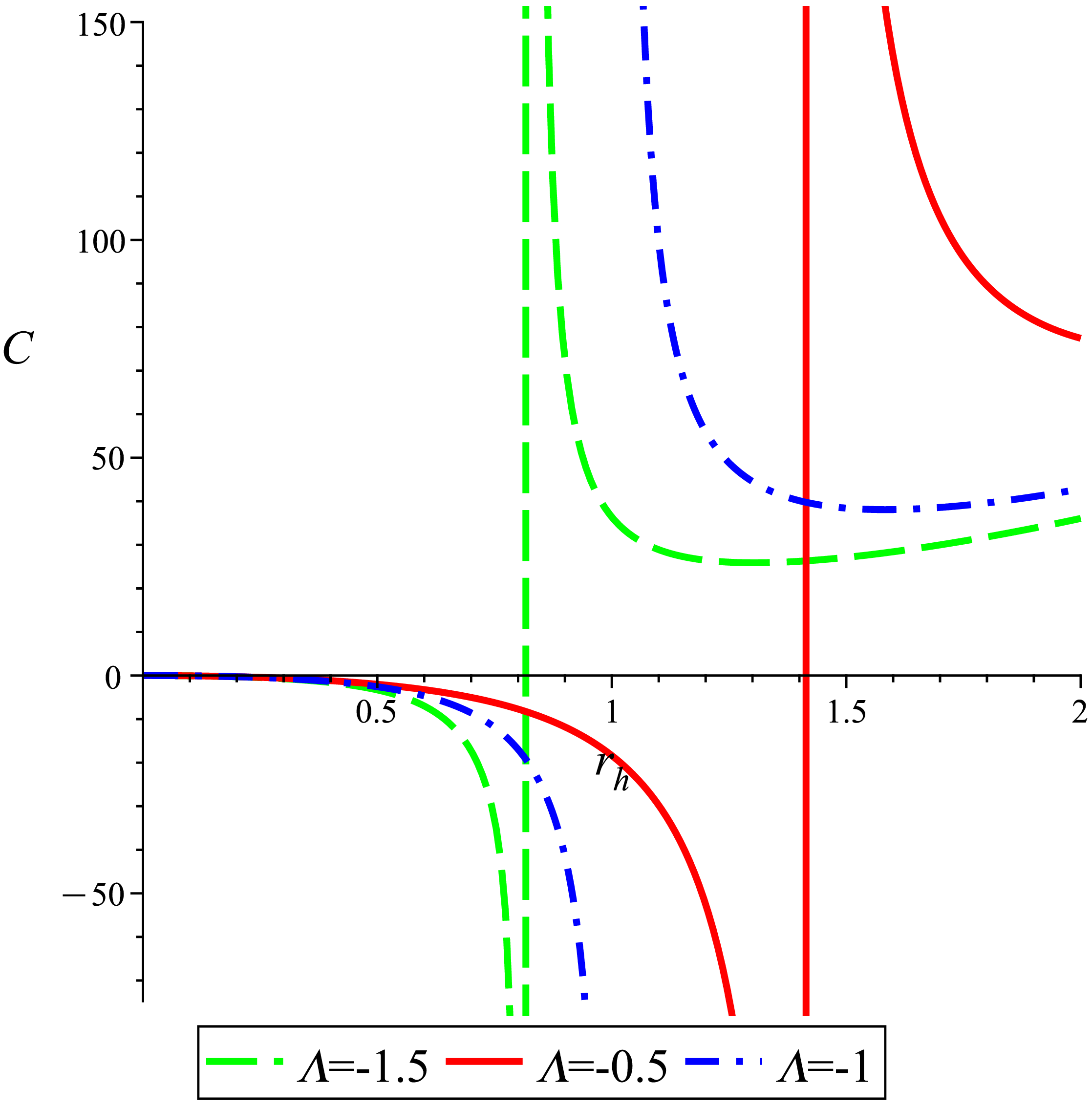
Now, we deal with the heat capacity which is proportional to the second derivative of the Gibbs free energy and can show the stability or instability of a system. The heat capacity at constant pressure up to the second order of takes the form
(45)
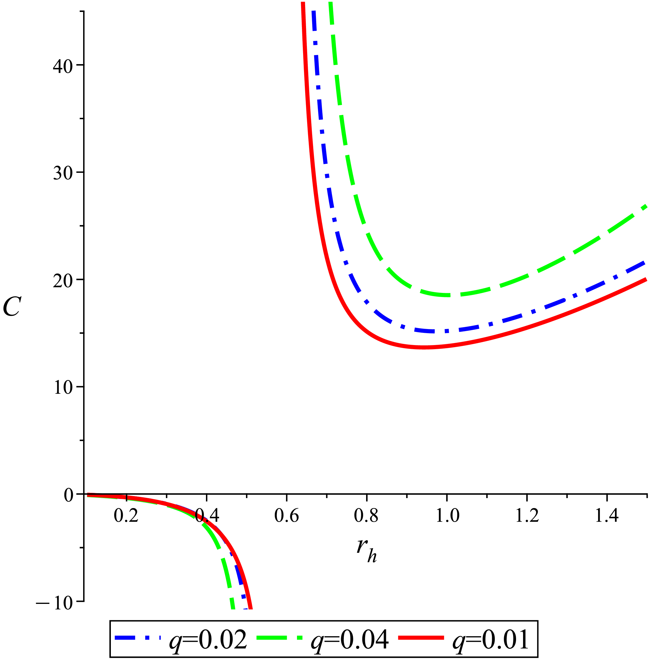
The denominator of (45) shows that the heat capacity diverges only at one point. The divergence point changes with changes in the pressure of the system. The interesting point is that the position of the divergence point does not change with the changes of the parameter . According to relation (45), the divergence point occurs at horizon . The heat capacity diagrams show that we have only two unstable and stable phases in this model, which correspond to small and large black holes. There is no intermediate phase in this model.
[a] [b]
Figure 7: The diagrams of the heat capacity versus the black hole horizon for different values of and ; (a): up to the second order of and (b): up to the third order of . By increasing the value of , the heat capacity diverges at smaller horizons.
[a] [b]
Figure 8: The diagrams of the heat capacity versus the black hole horizon for different values of and ; (a): up to the second order of and (b): up to the third order of . The divergence point is independent of the value of the parameter .
[a] [b]
Figure 9: The diagrams of the heat capacity versus the black hole temperature up to the second order of when, (a): changes and (b): the parameter changes. Different branches above and bellow the temperature axis show the stable and unstable black hole states.
Figures (7) and (8) represent the behavior of the heat capacity against the horizon of the black hole. As it is obvious, a transition between an unstable small black hole () to a large stable black hole () occurs. These divergence points in the diagrams of heat capacity can be signs of a second order phase transition. Because in the second order phase transition, the second derivative of the Gibbs free energy is discontinues. And the heat capacity is proportional to the second derivative of the Gibbs free energy. In the first order phase transition, the entropy which is proportional to the first derivative of the Gibbs free energy has a jump or varies suddenly at a point. Since. By increasing the value of , the phase transition takes place at smaller horizons. The right panels of figures (7) and (8) correspond to the heat capacity up to the second order of . In these cases, the heat capacity can have a root near the divergence points. In general, the roots indicate the phase transitions between stable and unstable phases in black holes. The divergence points are associated with critical behavior and phase transitions.
Figure (9) shows the behavior of heat capacity versus temperature. Two distinct branches in each plot refer to the two unstable(negative capacity) and stable(positive capacity) phases of the black hole. By increasing the value of , the diagram of the heat capacity diverges at higher temperatures. While, by increasing the value of , the heat capacity diverges at lower temperatures.
4 Conclusion
A general exponential modification for an AdS black hole action was considered. The solution for the metric function was obtained through a perturbative method up to the third order of the perturbation parameter. The behavior of the metric function for different values of parameters was depicted. Then, the thermodynamic behavior and phase transition of the black hole was studied. Through the thermodynamic study of this model we realized that the behavior of a Van der Waals fluid is not seen in this model. The necessary and important relations for the thermodynamic quantities were derived. The diagrams of the temperature versus the black hole horizon show behaviors like that of the Hawking-Page temperature diagrams and phase transitions between thermal AdS space and AdS black holes. The Smarr formula for this model was derived up to the linear order in . For this purpose, we had to consider the parameter as a thermodynamic variable conjugated to the potential . The entropy function against the black hole horizon does not behave abnormally up to the third order of , but from the fourth order of , for small horizons, the entropy increases. This cannot be explained classically. In this study, the diagrams of entropy versus temperature, show the sudden change in direction at specific points. This indicates a phase transition between the unstable and stable black hole states. The investigation of the Gibbs free energy versus temperature at constant pressure showed that it is possible to have a first-order phase transition in this model.In fact, the Gibbs free energy diagrams became very similar to the Gibbs diagrams of Hawking-Page transition. And as we know, the Hawking-Page transition is a transition of the first type. Also, the divergence points of the heat capacity signal a second order phase transition. The divergence points of the heat capacity depend only on and do not depend on the value of the parameter . Perhaps, by adding the matter field to the gravitational action, effects similar to the van der Waals fluid can be observed, which can be investigated in a separate work.
According to these results and the dictionary of AdS/CFT correspondence, we conclude that this model can be considered for the confinement-deconfinement phase transition and also a phase transition from a normal phase to a superconducting phase in the dual conformal field on the boundary of the AdS space.
Data Availability Data generated or analyzed during this study are provided in full within the published article.
Competing interests The authors declare that there are no competing interests.
References
[1]
K. S. Stelle,
Phys. Rev. D 16, 953-969 (1977).
[2]
C. Brans and R. H. Dicke,
Phys. Rev. 124, 925-935 (1961).
[3]
W. Hu and I. Sawicki,
Phys. Rev. D 76, 064004 (2007)
doi:10.1103/PhysRevD.76.064004
[arXiv:0705.1158 [astro-ph]].
[4]
S. Nojiri and S. D. Odintsov,
Phys. Rev. D 68 (2003), 123512
doi:10.1103/PhysRevD.68.123512
[arXiv:hep-th/0307288 [hep-th]].
[5]
D. Lovelock,
J. Math. Phys. 12, 498-501 (1971).
[6]
S. Nojiri and S. D. Odintsov,
Phys. Lett. B 631, 1-6 (2005)
doi:10.1016/j.physletb.2005.10.010
[arXiv:hep-th/0508049 [hep-th]].
[7]
M. Sadeghi and S. Parvizi,
Class. Quant. Grav. 33, no.3, 035005 (2016)
doi:10.1088/0264-9381/33/3/035005
[arXiv:1507.07183 [hep-th]].
[8]
S. Parvizi and M. Sadeghi,
Eur. Phys. J. C 79, no.2, 113 (2019)
doi:10.1140/epjc/s10052-019-6631-9
[arXiv:1704.00441 [hep-th]].
[9]
M. Fierz and W. Pauli,
Proc. Roy. Soc. Lond. A 173, 211-232 (1939)
doi:10.1098/rspa.1939.0140
[10]
C. de Rham,
Living Rev. Rel. 17, 7 (2014)
doi:10.12942/lrr-2014-7
[arXiv:1401.4173 [hep-th]].
[11]
M. Sadeghi,
Eur. Phys. J. C 78, no.10, 875 (2018)
doi:10.1140/epjc/s10052-018-6360-5
[arXiv:1810.09242 [hep-th]].
[12]
P. Rastall,
Phys. Rev. D 6, 3357-3359 (1972)
[13]
M. Sadeghi and F. Rahmani,
Int. J. Mod. Phys. A 38, no.20, 2350102 (2023)
doi:10.1142/S0217751X23501026
[arXiv:2301.12411 [hep-th]].
[14]
S. I. Kruglov,
Int. J. Mod. Phys. A 28, no.24, 1350119 (2013)
doi:10.1142/S0217751X13501194
[arXiv:1204.6709 [gr-qc]].
[15]
G. Cognola, E. Elizalde, S. Nojiri, S. D. Odintsov, L. Sebastiani and S. Zerbini,
Phys. Rev. D 77, 046009 (2008)
doi:10.1103/PhysRevD.77.046009
[arXiv:0712.4017 [hep-th]].
[16]
S. Nojiri and S. D. Odintsov,
Phys. Rept. 505, 59-144 (2011)
doi:10.1016/j.physrep.2011.04.001
[arXiv:1011.0544 [gr-qc]].
[17]
S. Nojiri, S. D. Odintsov and V. K. Oikonomou,
Phys. Rept. 692, 1-104 (2017)
doi:10.1016/j.physrep.2017.06.001
[arXiv:1705.11098 [gr-qc]].
[18]
J. M. Maldacena,
Adv. Theor. Math. Phys. 2 (1998), 231-252
[arXiv:hep-th/9711200 [hep-th]].
[19]
O. Aharony, S. S. Gubser, J. M. Maldacena, H. Ooguri and Y. Oz,
Phys. Rept. 323, 183-386 (2000)
doi:10.1016/S0370-1573(99)00083-6
[arXiv:hep-th/9905111 [hep-th]].
[20]
A. Dey, S. Mahapatra and T. Sarkar,
JHEP 01, 088 (2016)
doi:10.1007/JHEP01(2016)088
[arXiv:1510.00232 [hep-th]].
[21]
S. W. Hawking,
Nature 248, 30-31 (1974)
doi:10.1038/248030a0
[22]
R. M. Wald,
Phys. Rev. D 48, no.8, R3427-R3431 (1993)
doi:10.1103/PhysRevD.48.R3427
[arXiv:gr-qc/9307038 [gr-qc]].
[23]
B. P. Dolan,
Class. Quant. Grav. 28, 125020 (2011)
doi:10.1088/0264-9381/28/12/125020
[arXiv:1008.5023 [gr-qc]].
 [b]
[b]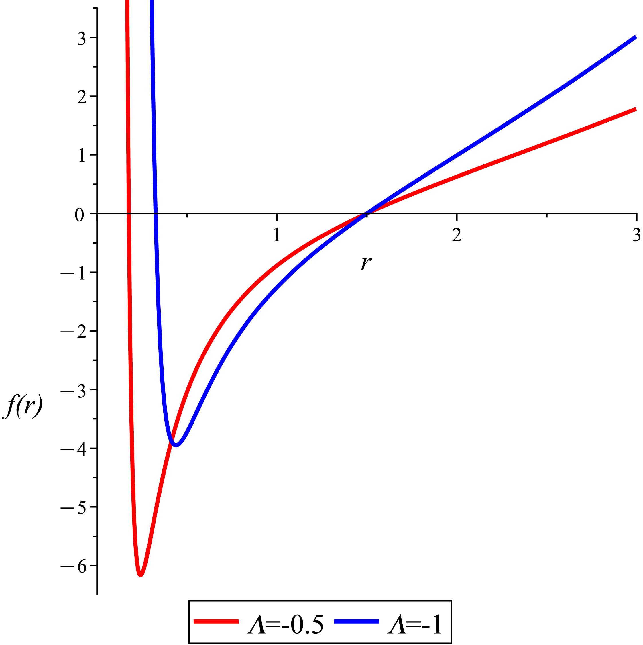
 [b]
[b]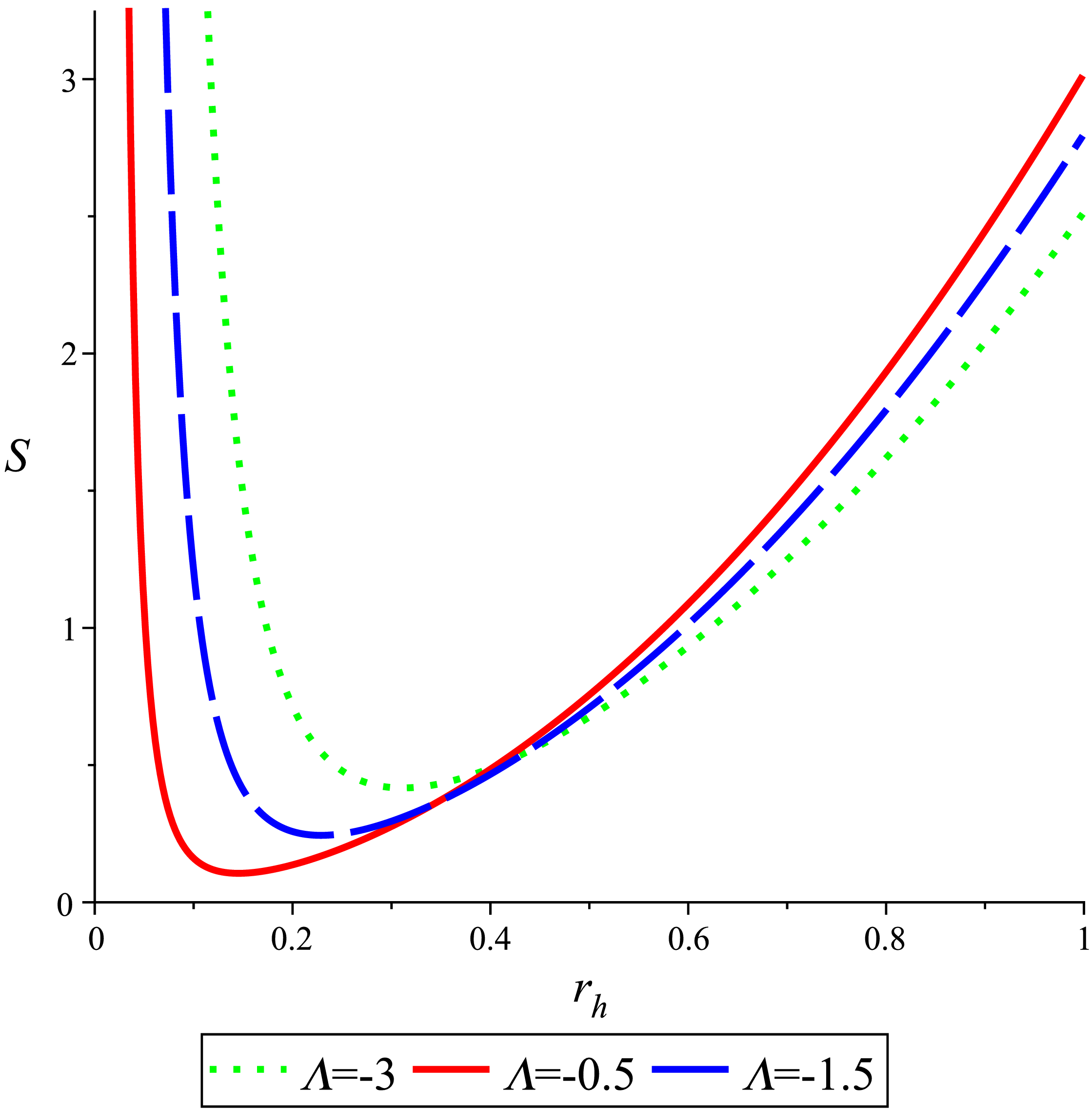
 [b]
[b]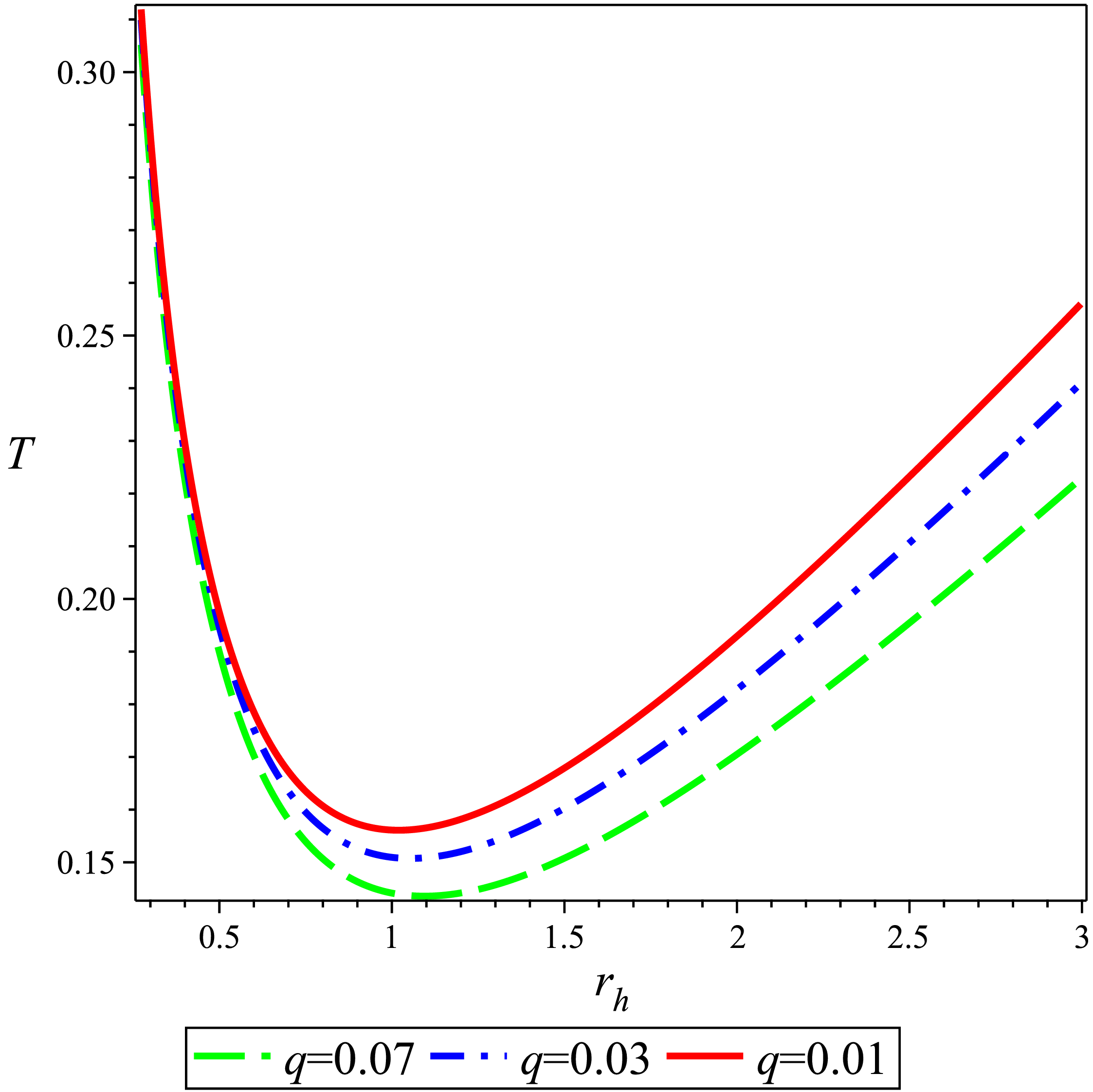
 [b]
[b]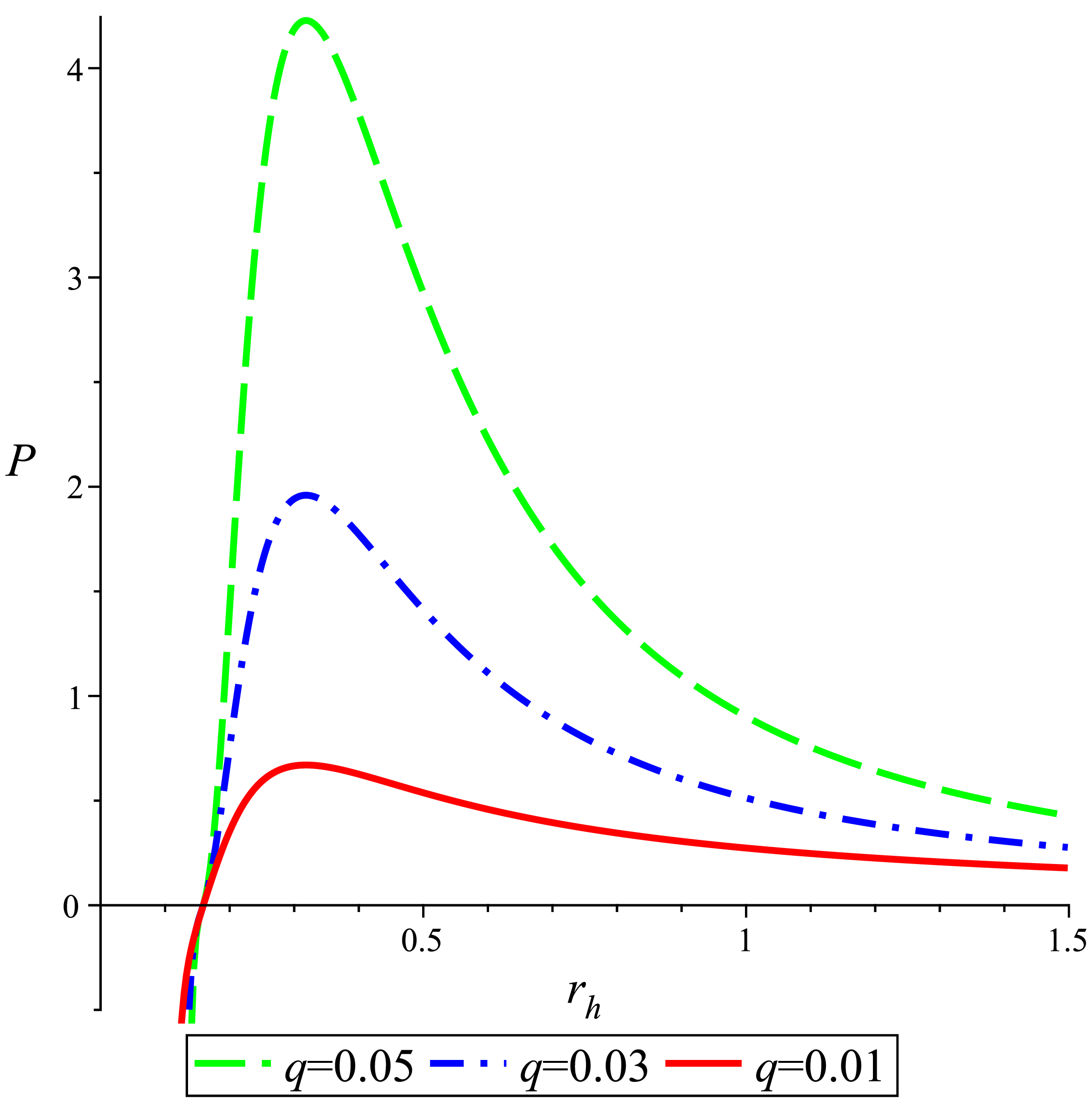
 [b]
[b]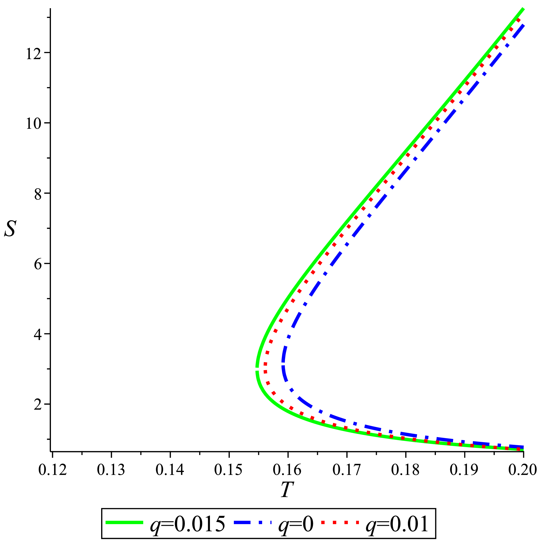
 [b]
[b]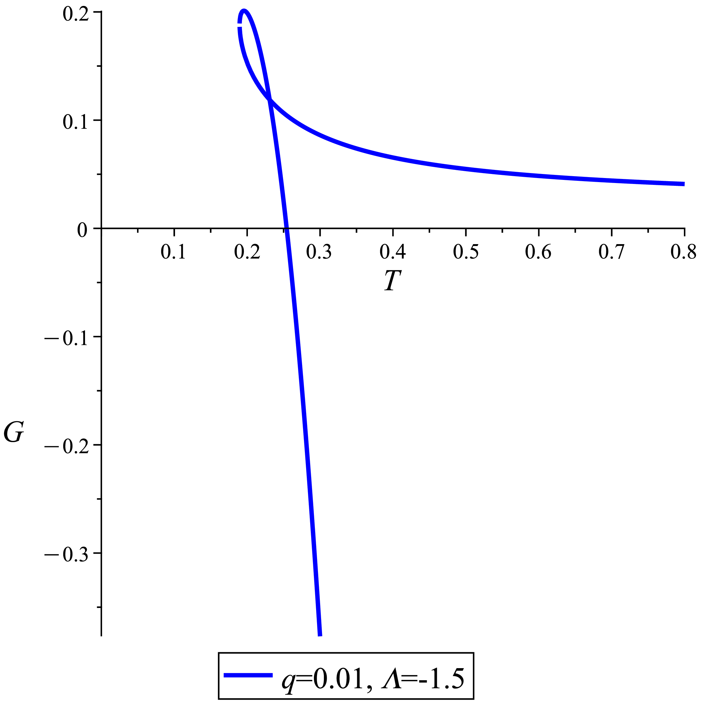 [c]
[c]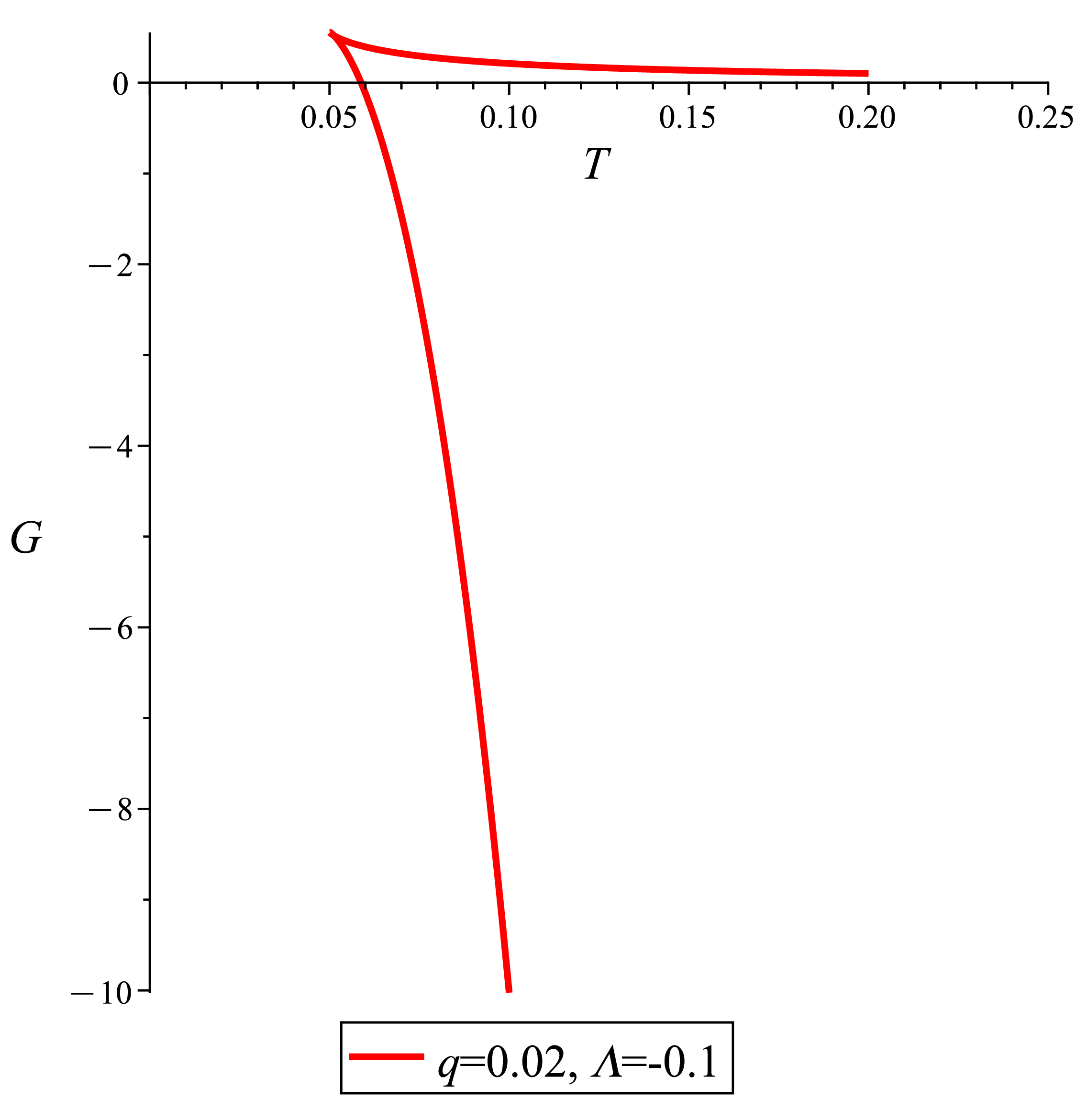 [d]
[d]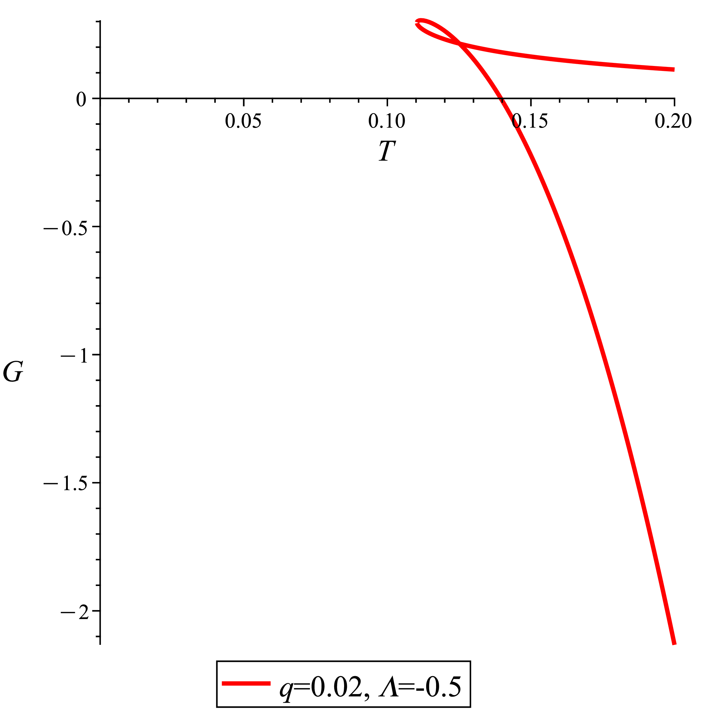
 [b]
[b]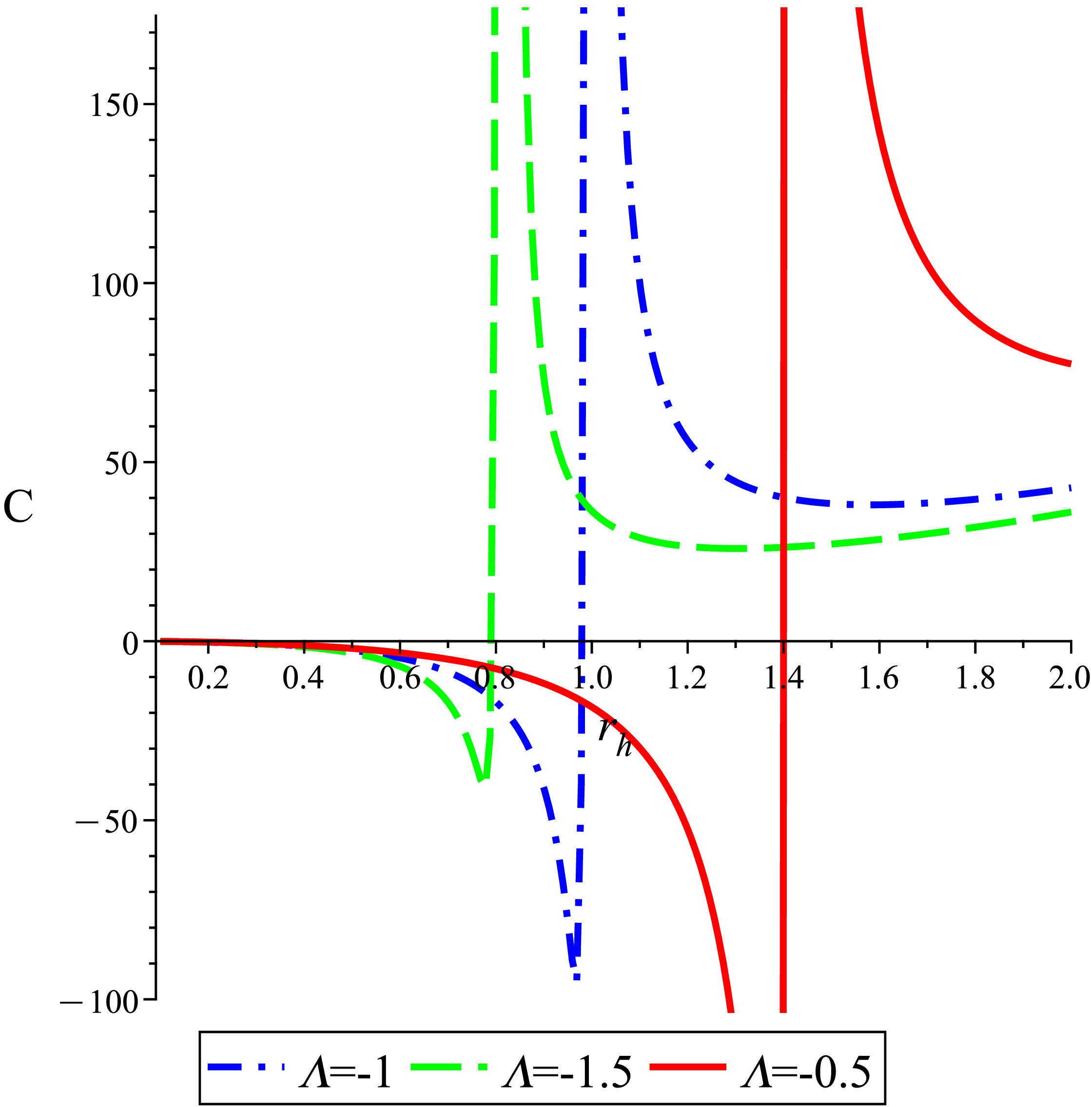
 [b]
[b]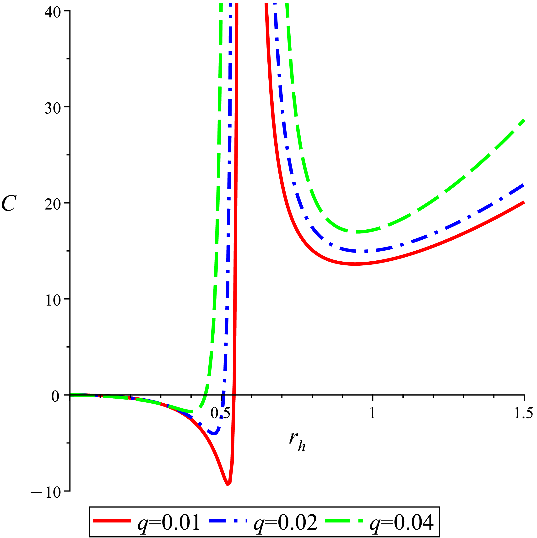
 [b]
[b]