Entanglement distribution based on quantum walk in arbitrary quantum networks

Abstract

In large-scale quantum networks, distributing the multi-particle entangled state among selected nodes is crucial for realizing long-distance and complicated quantum communication. Quantum repeaters provides an efficient method to generate entanglement between distant nodes. However, it is difficult to extend quantum repeater protocols to high-dimensional quantum states in existing experiments. Here we develop a series of scheme for generating high-dimensional entangled states via quantum walks with multiple coins or single coin by quantum repeaters, including $d$-dimensional Bell states, multi-particle high dimensional GHZ states etc.. Furthermore, we give entanglement distribution schemes on arbitrary quantum networks according to the above theoretical framework. As applications, we construct quantum fractal networks and multiparty quantum secret sharing protocols based on $d$-dimensional GHZ states. In the end, we give the experiment implementing of various 2-party or 3-party entanglement generation schemes based on repeaters. Our work can serve as a building block for constructing larger and more complex quantum networks.

1 Introduction

Quantum networks holds great potential for realizing various quantum technologies, including secure communication schemes, distributed quantum computing, and metrological applications [1, 2, 3]. However, how to construct large-scale quantum networks and realize long-distance quantum communication is one of the most challenging tasks in practical quantum information technology [4]. Entanglement[5], as a very powerful and efficient quantum resource, is the cornerstone of many quantum communication and quantum computing protocols[6, 7, 8, 9]. The quantum network’s foundation relies on entangled distributions between nodes, yet creating such distributions over long distances at high data rates remains challenging due to quantum information degradation during transmission. Quantum repeaters offer a potential solution by amplifying quantum signals while adhering to quantum physics principles. In practice, quantum repeaters are designed to avoid exponential decay in the success rate or fidelity of quantum information or entangled states by sending light through lossy quantum channels for processing[10, 11, 12]. The core idea of quantum repeater is based on the technique of entanglement swapping, which operates by consolidating multiple short-distance entanglements to generate a unified long-distance entanglement.

The experimental implementation of quantum repeater has witnessed significant advancements in recent years [13], which mainly has two frameworks - one with quantum memory and the other without [14, 15].DLCZ scheme [14], one of the well-known quantum repeater protocols, is a method that uses collective spin excitation in an atomic ensemble[16] to provide the required quantum memory and the heralded entanglement connection is used to boost the scaling of efficiency through the memory enhancement. In addition to using the ensemble system as a quantum memory, there are also single atomic ions or diamond defect spins[17, 18, 19, 20, 21]. Another famous experimental scheme proposes all-photonic quantum repeaters to avoid the need for quantum memory by exploiting the graph state in the repeater nodes[15]. So far, the quantum repeater protocol has been experimentally implemented in many physical systems. However, due to some challenges of existing experimental techniques, such as performing deterministic high-dimensional multi-particle GHZ state measurements[22], the connected entangled states are all 2-dimensional two-particle quantum states[23], and it is difficult to extend to high-dimensional multi-particle quantum states in existing experiments. Compared to the conventional two-level systems, high-dimensional states can offer extended possibilities such as both higher capacity and noise resilience in quantum communications[24, 25], larger violation of Bell inequality[26], as well as more efficient quantum simulation [27] and computation[28]. Although there are many existing studies on qubit quantum repeaters, less attention has been paid to qudit quantum repeaters for quantum entanglement and long-distance distribution of information.

Quantum walks, as a framework combining quantum theory and classical random walk, [29, 30, 31] play an important role in quantum information processing, especially for 2-dimensional and high-dimensional quantum teleportation[32] and entangled state generation[33]. Being a universal quantum computing model[34, 35], quantum walks can be experimentally realized in many physical systems, including trapped ions[36, 37], nuclear magnetic resonance [38], photonics[39, 40], neutral atoms[41], Bose-Einstein condensates[42, 43], cavity quantum electrodynamics[44], superconducting qubits[45], etc. And some of them can be extended to high-dimensional experimental protocol for quantum walks[37, 42]. Obviously, quantum walks holds significant potential in the implementation of quantum repeater networks[46]. In this paper, based on quantum walk with multiple coins[47] or single coin, we propose a series of quantum repeater protocols to generate high-dimensional entangled Bell states and GHZ states which can avoid high-dimensional bell measurement and multi-particle GHZ measurement, and then extend to the entangled distribution on arbitrary quantum networks. At the same time, we give experiment implementation on superconducting quantum computer Quafu ScQ-P10. Especially, to our knowledge, we firstly give experimental implementation of the generation of two-party entangled GHZ states using two GHZ states, and three-party entangled GHZ states using three Bell or GHZ states. In the end, we give some applications of our entanglement distribution on quantum fractal networks and multiparty quantum secret sharing protocol. Since quantum walks is a universal quantum computing model, which provides a versatile platform to establish quantum network.

The paper is organized as follows. First, we will briefly introduce the model of quantum repeaters and quantum walks with multiple coins in section 2. Next we give theoretical schemes based on quantum walks that can generate 2-dimensional and high-dimensional quantum entangled state for quantum repeaters including Bell state, GHZ state with arbitrary particle number in section 3. In section 4, we give our entanglement distribution scheme on arbitrary quantum networks according to the above theoretical schemes. In section 5, we construct quantum fractal networks and multiparty quantum secret sharing protocols based on d-dimensional GHZ states as applications. In the section 6, we give the experiment implementing of various entanglement generation schemes. Finally, we make a summary and outlook in section 7.

2 Preliminary

2.1 Quantum repeater model.

The quantum repeater plays a crucial role in the establishment of long-distance quantum communication. In a quantum repeater scheme, the communication channel is divided into $N$ segments, with connection points or auxiliary nodes interspersed. $N$ elementary entangled states are created between nodes $A$ and $C_{1}$, $C_{1}$ and $C_{2}$,…,$C_{N-1}$ and $B$, refer to Figure 1. Every pair of neighboring elementary entangled states is connected using methods such as Bell measurements at intermediary nodes enabling the creation of new entangled states between more distant nodes, reminiscent of entanglement swapping schemes. Importantly, elementary entangled states encompass not only EPR pairs but also $d$-dimensional Bell states or GHZ states. The use of the $d$-dimensional Bell state allows for high-dimensional quantum communication with increased message capacity, while GHZ states exhibit enhanced robustness under local decoherence[48].

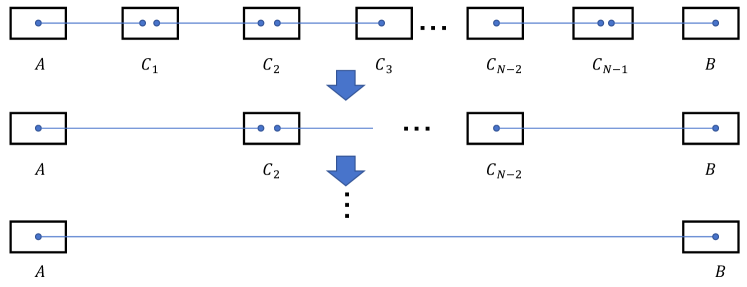
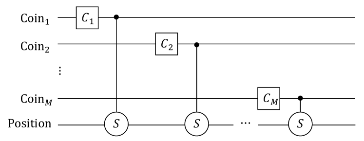
Figure 1: (a) The model of the quantum repeater. Black squares represent nodes labeled as $A,C_{1},\cdots,C_{N-1},B$, and blue line segments depict entangled states between two nodes. After rounds of connection and purification operations, entangled states between two distant nodes will be generated, ultimately resulting in an entangled state between nodes $A$ and $B$. (b) The circuit schematic diagram of quantum walk with $M$ coins. The first $M$ horizontal lines represent the coin states, and the last line represents the position state. $C_{i}$ is the coin operator acting on the $i$-th coin space. $S$ is the shift operator acting on the combination space of the position and the coin space.

This paper primarily focuses on the connection process of a quantum repeater, emphasizing the generation of a quantum entangled state between more distant nodes through quantum walks with either a single coin or multiple coins.

2.2 Quantum walks with multiple coins on complete graphs.

A quantum walk with $M$ coins on the $d$-complete graph takes place in a compound Hilbert space comprising a position space and $M$ coin spaces, i.e. $\mathcal{H}=\mathcal{H}_{C_{1}}\otimes\cdots\otimes\mathcal{H}_{C_{M}}\otimes\mathcal{H}_{P}$, where $\mathcal{H}_{P}=span\{|n\rangle:n=0,1,\cdots d-1\}$, and $|n\rangle$ is the position state corresponding to the vertex $n$ on the $d$-completed graph. At each vertex $n$, there are $d$ directed edges with labels $\{0,1,\cdots d-1\}$ pointing to other vertices. For any coin space, $\mathcal{H}_{C_{m}}=span\{|a\rangle:a=0,1,\cdots d-1\},m=1,2,\cdots,M$, and $|a\rangle$ is the coin state corresponding to the edge $a$. The conditional shift operator acting on the $m$-th coin space is given by $S=\sum\limits_{k,j=0}^{d-1}|k\rangle_{m}\langle k|\otimes|j-k\rangle_{P}\langle j|$. Especially, when $d=2$, the $\mathcal{H}_{P}=span\{|0\rangle,|1\rangle\}$, and $\mathcal{H}_{C_{m}}=span\{|0\rangle,|1\rangle\},m=1,2,\cdots,M$. The conditional shift operator $S^{2-complete}$ of the quantum walk on $2$-complete graph is a Controlled-NOT gate.

Thus the $m$-th step quantum walk is described as $W_{m}=S(I\otimes C_{m})$, where the coin operator $C_{m}$ and the identify operator $I$ act on the coin spaces. The conditional shift operator $S$ acts on the space ${H}_{C_{m}}\otimes\mathcal{H}_{P}$. The circuit diagram of this quantum walk can be seen in Figure 1.

The entanglement generation framework by quantum walks proposed in reference [33] exhibits notable differences when compared to the current model. In order to generate distant entanglement, the current scheme maybe show better advantages. Refer to Figure 2 and Figure 2, the design choice of local operations in current scheme enhances the adaptability of quantum walks to the quantum repeater model.

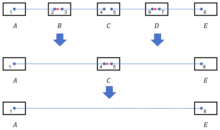
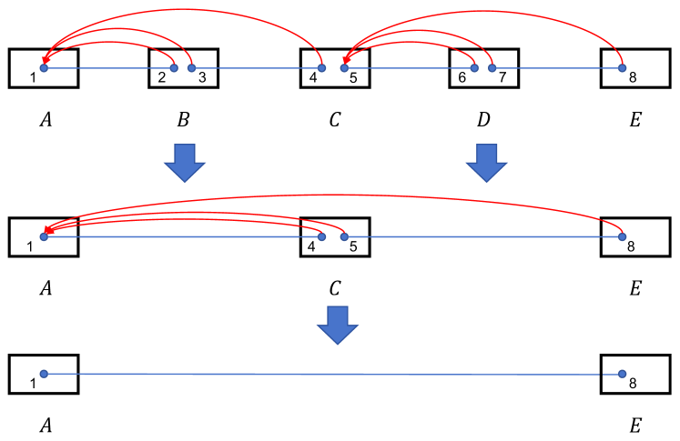
Figure 2: The schematic diagrams of our entanglement generation schemes and the entanglement generation schemes proposed by [33], respectively. Black squares represent nodes labelled as $A,B,C,D,E$, blue line segment represent entangled state between two nodes. The red arrows within a square symbolize quantum walk operations, with their origin points denoting coin states and their destination points corresponding to position states. (a) Our scheme can achieve particles 1 and 4 entanglement through a quantum walk between particles 2 and 3 inside a node $B$. By repeating the same steps, we can obtain quantum entangled states over longer distances, such as the quantum entangled state between particles 1 and 8. (b) According to the entanglement generation schemes proposed by [33], we should perform three steps of the quantum walk among nodes $A,B,C$ with particles 2, 3 and 4 being coin states in turn and particle 1 being the position state to entangle particle 1 and 4. Similarly, We need perform quantum walk operators among nodes $A,C,E$ entangle particle 1 and 8, which are long-distance quantum operations disallowed by a quantum repeater.

3 Entanglement generation of quantum states

In the following, we will introduce entanglement generation scheme by quantum walks with multiple coins on $d$-complete graph.

3.1 2-dimensional quantum states

2-dimensional Bell states

First, a $2$-dimensional Bell state $|\Phi^{+}\rangle=\frac{|00\rangle+|11\rangle}{\sqrt{2}}$ can be generated by quantum walks with a single coin through two $2$-dimensional Bell states. Let the initial state be

$$|\Psi(0)\rangle=\frac{|00\rangle+|11\rangle}{\sqrt{2}}_{1,2}\otimes\frac{|00\rangle+|11\rangle}{\sqrt{2}}_{3,4}$$ (1)

and the particles $2$ and $3$ be the coin state and the position state, respectively. The coin operator is set as $C=X$, and the conditional shift operator is the CNOT gate. Then the quantum state after one step of the quantum walk is

$$|\Psi_{1}\rangle=\frac{1}{2}(|0110\rangle+|0101\rangle+|1000\rangle+|1011\rangle)_{1,2,3,4}$$ (2)

$$=\frac{1}{2\sqrt{2}}(|0+10\rangle-|0-10\rangle+|0+01\rangle-|0-01\rangle$$

$$+|1+00\rangle+|1-00\rangle+|1+11\rangle+|1-11\rangle)_{1,2,3,4}.$$ (3)

Then, we take a measurement with the basis $\{|+\rangle,|-\rangle\}$ and $\{|0\rangle,|1\rangle\}$ in the particles $2$ and $3$, where the corresponding measurement results of $|\pm\rangle=\frac{|0\rangle\pm|1\rangle}{\sqrt{2}}$ are $0$ and $1$, respectively. The entanglement states of the particles $1$ and $4$ corresponding to different measurement results are shown in the Table 1, which can be recovered to the state $|\Phi^{+}\rangle$ by some local unitary operations according to the measurement results.

Measurement	Entanglement	Local
results	states	operations
00	$\frac{1}{\sqrt{2}}(|01\rangle+|10\rangle)$	$X_{1}$
01	$\frac{1}{\sqrt{2}}(|00\rangle+|11\rangle)$	$I_{1}$
10	$\frac{1}{\sqrt{2}}(|10\rangle-|01\rangle)$	$Z_{1}X_{1}$
11	$\frac{1}{\sqrt{2}}(|11\rangle-|00\rangle)$	$-Z_{1}$

Table 1: Entangled states of the particles $1$ and $4$. The measurement results of the particles $2$ and $3$ are shown in the first column. The second column represents the entangled states of the particles $1$ and $4$ corresponding to different measurement results. The third column represents the local unitary operations on the particle $1$ recovering the state of particles $1$ and $4$ to $|\Phi^{+}\rangle$.

2-dimensional 3-qubit GHZ states

A $2$-dimensional GHZ states $\frac{|000\rangle+|111\rangle}{\sqrt{2}}$ can be generated by quantum walks with two coins through two $2$-dimensional GHZ states.

Let the initial state be

$$|\Psi(0)\rangle=\frac{|000\rangle+|111\rangle}{\sqrt{2}}_{1,2,3}\otimes\frac{|000\rangle+|111\rangle}{\sqrt{2}}_{4,5,6}$$ (4)

and the particles $2$ and $3$ be the coin states and the particle $4$ be the position state, respectively. The coin operators are set as $C_{1}=X,C_{2}=H$, and the conditional shift operator $S$ is the CNOT gate. Then the quantum state after two steps of the quantum walk is

$$|\Psi_{1}\rangle=\frac{1}{4}(|0+0011\rangle+|0+0100\rangle+|0+1000\rangle$$

$$+|0+1111\rangle-|0-0011\rangle-|0-0100\rangle-|0-1000\rangle$$

$$-|0-1111\rangle+|1+0000\rangle+|1+0111\rangle-|1+1011\rangle$$

$$-|1+1100\rangle+|1-0000\rangle+|1-0111\rangle-|1-1011\rangle$$

$$-|1-1100\rangle)_{1,2,3,4,5,6}.$$ (5)

Then, we take a measurement with the basis $\{|+\rangle,|-\rangle\}$ in the particle $2$ and the basis $\{|0\rangle,|1\rangle\}$ in the particles $3$ and $4$. The entanglement states of the particles $1,5$ and $6$ corresponding to different measurement results are shown in the Table 2, which can be recovered to the state $\frac{|000\rangle+|111\rangle}{\sqrt{2}}$ by some local unitary operations according to the measurement results. Thus we can take GHZ states as elementary entangled states of a quantum repeater by this scheme to generate a distant entangled state among some nodes, such as the generation process shown in Figure 3.

Measurement	Entanglement	Local
results	states	operations
000	$\frac{1}{\sqrt{2}}(|011\rangle+|100\rangle)$	$X_{1}$
001	$\frac{1}{\sqrt{2}}(|000\rangle+|111\rangle)$	$I_{1}$
010	$\frac{1}{\sqrt{2}}(|000\rangle-|111\rangle)$	$Z_{1}$
011	$\frac{1}{\sqrt{2}}(|011\rangle-|100\rangle)$	$X_{1}Z_{1}$
100	$\frac{1}{\sqrt{2}}(-|011\rangle+|100\rangle)$	$Z_{1}X_{1}$
101	$\frac{1}{\sqrt{2}}(-|000\rangle+|111\rangle)$	$-Z_{1}$
110	$\frac{1}{\sqrt{2}}(-|000\rangle-|111\rangle)$	$-I_{1}$
111	$\frac{1}{\sqrt{2}}(-|011\rangle-|100\rangle)$	$-X_{1}$

Table 2: Entangled states of the particles $1,5$ and $6$. The measurement results of the particles $2,3$ and $4$ are shown in the first column. The second column represents the entangled states of the particles $1,5$ and $6$ corresponding to different measurement results. The third column represents the local unitary operations on the particle $1$ recovering the state of particles $1,5$ and $6$ to $\frac{|000\rangle+|111\rangle}{\sqrt{2}}$.

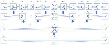
Figure 3: The schematic diagram of the generation process of a GHZ state among three nodes. Squares represent quantum nodes, and triangles represent GHZ states. Arrows in a square represent quantum walk operations with start points and target points being coin states and position states, respectively. After several quantum walk operations at middle nodes, we will generate a GHZ state among nodes $A$, $B$ and $C$.

2-dimensional multi-qubit GHZ states

Now we extend the above results to generate the multi-qubit GHZ states, i.e. $\frac{|00\cdots 0\rangle+|11\cdots 1\rangle}{\sqrt{2}}$. We can use two models: quantum walks with multiple coins and parallel quantum walks with a single coin which are shown in the Figure 4 and Figure 4, respectively.

Method 1: Let the initial state be

$$|\Psi(0)\rangle=\frac{|0\cdots 00\cdots 0\rangle+|1\cdots 11\cdots 1\rangle}{\sqrt{2}}_{a_{1},\cdots,a_{k},a_{k+1},\cdots,a_{m}}$$

$$\otimes\frac{|00\cdots 0\rangle+|11\cdots 1\rangle}{\sqrt{2}}_{b_{1},b_{2},\cdots,b_{n}}$$ (6)

and the particles $a_{1},a_{2},\cdots,a_{k}$ be the coin states and the particle $b_{1}$ be the position state, respectively, to perform a quantum walk with multiple coins. Set the coin operators as $C_{1}=X,C_{2}=C_{3}=\cdots=C_{k}=H$, and the conditional shift operator $S$ as the CNOT gate. Then the quantum state after the first step of the quantum walk is

$$|\Psi(1)\rangle=\frac{1}{2}(|10\cdots 00\cdots 010\cdots 0\rangle$$

$$+|10\cdots 00\cdots 001\cdots 1\rangle+|01\cdots 11\cdots 100\cdots 0\rangle$$ (7)

$$+|01\cdots 11\cdots 111\cdots 1\rangle)_{a_{1},a_{2},\cdots,a_{k},a_{k+1},\cdots,a_{m},b_{1},b_{2},\cdots,b_{n}}.$$

After the remaining $k-1$ steps of the quantum walk, the quantum state is

$$|\Psi(k)\rangle =\frac{1}{(\sqrt{2})^{k+1}}\sum\limits_{x_{2},\cdots x_{k}=0}^{1}(|1x_{2}\cdots x_{k}0\cdots 0\overline{y}0\cdots 0\rangle$$

$$+|1x_{2}\cdots x_{k}0\cdots 0y1\cdots 1\rangle$$

$$+(-1)^{y}|0x_{2}\cdots x_{k}1\cdots 1y0\cdots 0\rangle$$

$$+(-1)^{y}|0x_{2}\cdots x_{k}1\cdots 1\overline{y}1\cdots 1\rangle)$$ (8)

where $y=(x_{2}+\cdots+x_{k})$ mod 2. Then, we take a measurement with the basis $\{|+\rangle,|-\rangle\}$ in the particle $a_{1}$ and the basis $\{|0\rangle,|1\rangle\}$ in the particles $a_{2},\cdots,a_{k}$ and $b_{1}$. The entanglement states of the particles $a_{k+1},\cdots,a_{m}$ and $b_{2},\cdots,b_{n}$ corresponding to different measurement results are shown in the Table 3, which can be recovered to the state $\frac{|0\cdots 0\rangle+|1\cdots 1\rangle}{\sqrt{2}}$ by some local unitary operations according to the measurement results. If we only measure the particles $a_{2},\cdots,a_{k}$ and $b_{1}$, we also can obtain a GHZ state through local unitary operations according to $|\Psi(k)\rangle$ and measurement results.

Measurement	Entanglement	Local
results	states	operations
$0x_{2}\cdots x_{k}y$	$\frac{1}{\sqrt{2}}(|0\cdots 01\cdots 1\rangle$
	$+(-1)^{y}|1\cdots 10\cdots 0\rangle)$	$X_{k+1}\cdots X_{m}Z_{k+1}^{y}$
$0x_{2}\cdots x_{k}\overline{y}$	$\frac{1}{\sqrt{2}}(|0\cdots 00\cdots 0\rangle$
	$+(-1)^{y}|1\cdots 11\cdots 1\rangle)$	$Z_{k+1}^{y}$
$1x_{2}\cdots x_{k}y$	$\frac{1}{\sqrt{2}}(-|0\cdots 01\cdots 1\rangle$
	$+(-1)^{y}|1\cdots 10\cdots 0\rangle)$	$-X_{k+1}\cdots X_{m}Z_{k+1}^{y+1}$
$1x_{2}\cdots x_{k}\overline{y}$	$\frac{1}{\sqrt{2}}(-|0\cdots 00\cdots 0\rangle$
	$+(-1)^{y}|1\cdots 11\cdots 1\rangle)$	$-Z_{k+1}^{y+1}$

Table 3: Entangled states of the particles $a_{k+1},\cdots,a_{m}$ and $b_{2},\cdots,b_{n}$. The measurement results of the particles $a_{1},\cdots,a_{k}$ and $b_{1}$ are shown in the first column. The second column represents the entangled states of the particles $a_{k+1},\cdots,a_{m}$ and $b_{2},\cdots,b_{n}$ corresponding to different measurement results. The third column represents the local unitary operations on the particle $a_{k+1},\cdots,a_{m}$ recovering the state of particles $a_{k+1},\cdots,a_{m}$ and $b_{2},\cdots,b_{n}$ to $\frac{|0\cdots 0\rangle+|1\cdots 1\rangle}{\sqrt{2}}$.

Method 2: The initial state is

$$|\Psi(0)\rangle=\frac{|0\cdots 00\cdots 0\rangle+|1\cdots 11\cdots 1\rangle}{\sqrt{2}}_{a_{1},\cdots,a_{k},a_{k+1},\cdots,a_{m}}$$

$$\otimes\frac{|0\cdots 00\cdots 0\rangle+|1\cdots 11\cdots 1\rangle}{\sqrt{2}}_{b_{1},\cdots b_{k},b_{k+1},\cdots,b_{n}}.$$ (9)

Let the particles $a_{1},\cdots,a_{k}$ be the coin states and the particle $b_{1},\cdots,b_{k}$ be the corresponding position state, respectively, to perform $k$ parallel quantum walks with a single coin. Set the coin operators as $C=X$, and the conditional shift operator $S$ as the CNOT gate. Then the quantum state after the $k$ parallel quantum walks is

$$|\Psi(1)\rangle=\frac{1}{2}(|1\cdots 10\cdots 01\cdots 10\cdots 0\rangle$$

$$+|1\cdots 10\cdots 00\cdots 01\cdots 1\rangle+|0\cdots 01\cdots 10\cdots 00\cdots 0\rangle$$

$$+|0\cdots 01\cdots 11\cdots 11\cdots 1\rangle).$$ (10)

Then, we take a measurement with the basis $\{|+\rangle,|-\rangle\}$ in the particle $a_{1},\cdots,a_{k}$ and the basis $\{|0\rangle,|1\rangle\}$ in the particles $b_{1},\cdots,b_{k}$. The entanglement states of the particles $a_{k+1},\cdots,a_{m}$ and $b_{k+1},\cdots,b_{n}$ corresponding to different measurement results are shown in the Table 4, which can be recovered to the state $\frac{|0\cdots 0\rangle+|1\cdots 1\rangle}{\sqrt{2}}$ by some local unitary operations according to the measurement results. If we only measure the particles $b_{1},\cdots,b_{k}$ in the method $2$, we also can obtain a GHZ state through local unitary operations. Thus we can change the particles be measured according to the actual demand to implement the entanglement swapping we need.

Measurement	Entanglement	Local
results	states	operations
$x_{1}\cdots x_{k}$	$\frac{1}{\sqrt{2}}((-1)^{N}|0\cdots 01\cdots 1\rangle$
$0\cdots 0$	$+|1\cdots 10\cdots 0\rangle)$	$(-Z_{k+1})^{N}$
$x_{1}\cdots x_{k}$	$\frac{1}{\sqrt{2}}((-1)^{N}|0\cdots 00\cdots 0\rangle$	$X_{k+1}$
$1\cdots 1$	$+|1\cdots 11\cdots 1\rangle)$	$\cdots X_{m}(-Z_{k+1})^{N}$

Table 4: Entangled states of the particles $a_{k+1},\cdots,a_{m}$ and $b_{k+1},\cdots,b_{n}$. The measurement results of the particles $a_{1},\cdots,a_{k}$ and $b_{1},\cdots,b_{k}$ are shown in the first column, where $x_{1},\cdots,x_{k}$ are the measurement results of the particles $a_{1},\cdots,a_{k}$. The second column represents the entangled states of the particles $a_{k+1},\cdots,a_{m}$ and $b_{k+1},\cdots,b_{n}$ corresponding to different measurement results, where $N=(x_{1}+\cdots+x_{k})$ mod 2. The third column represents the local unitary operations on the particle $a_{k+1},\cdots,a_{m}$ recovering the state of particles $a_{k+1},\cdots,a_{m}$ and $b_{k+1},\cdots,b_{n}$ to $\frac{|0\cdots 0\rangle+|1\cdots 1\rangle}{\sqrt{2}}$.

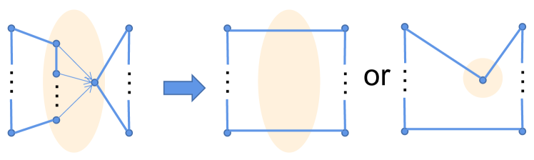
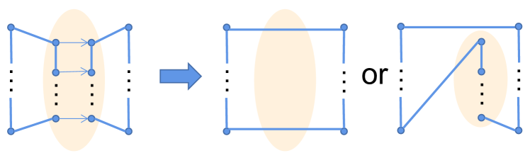
Figure 4: (a)-(b) The operation process schematic diagrams of method $1$ and method $2$. The blue polygons represent $2$-dimensional GHZ states, where the vertices represent qubits. The arrows within the yellow region denote quantum walk operations, where the initial and final points correspond to coin states and position states, respectively. (a) After performing quantum walk and measurement operations, we will generate a GHZ state among qubits located outside the yellow region or between qubits outside the yellow region and one qubit within the yellow region. (b) we will generate a GHZ state among qubits located outside the yellow area or between qubits outside the yellow area and $k$ qubits within yellow area. (c) The schematic diagram illustrates the operational process of simultaneously employing the aforementioned two methods to generate a GHZ state. The blue polygons represent $2$-dimensional GHZ states, with the vertices representing qubits. The arrows in the green and pink areas indicate the quantum walk operations in method $1$ and method $2$, respectively. After performing quantum walk and measurement operations, we will generate a GHZ state among qubits outside the two areas.

The above two methods respectively obtain $m+n-(k+1)$ and $m+n-2k$ qubits GHZ states from two GHZ states with $m$ and $n$ qubits, respectively. More generally, we can obtain GHZ states with $m+n-q,2\leq q\leq m+n-2$ qubits through using the above two methods simultaneously as shown in Figure 4. Specifically, for the initial state

$$|\Psi(0)\rangle=\frac{|0\cdots 00\cdots 0\rangle+|1\cdots 11\cdots 1\rangle}{\sqrt{2}}_{a_{1},\cdots,a_{k},a_{k+1},\cdots,a_{m}}$$

$$\otimes\frac{|0\cdots 00\cdots 0\rangle+|1\cdots 11\cdots 1\rangle}{\sqrt{2}}_{b_{1},\cdots,b_{l},b_{l+1},\cdots,b_{n}},$$ (11)

without losing generality, we can assume $k>l\geq 2$ and $k+l=q$. We use the method 2 in the particles $a_{1},\cdots,a_{l-1}$ and $b_{1},\cdots,b_{l-1}$, and use the method 1 in the particles $a_{l},\cdots,a_{k}$ and $b_{l}$. Thus the initial quantum state becomes

$$|\Psi(1)\rangle=\frac{1}{(\sqrt{2})^{k-l}}\sum\limits_{x_{l+1},\cdots,x_{k}=0}^{1}(|1\cdots 11x_{l+1}\cdots x_{k}0\cdots 0\rangle$$

$$\otimes|1\cdots 1\overline{y}0\cdots 0\rangle+|1\cdots 11x_{l+1}\cdots x_{k}0\cdots 0\rangle$$

$$\otimes|0\cdots 0y1\cdots 1\rangle+(-1)^{y}|0\cdots 00x_{l+1}\cdots x_{k}1\cdots 1\rangle$$

$$\otimes|0\cdots 0y0\cdots 0\rangle+(-1)^{y}|0\cdots 00x_{l+1}\cdots x_{k}1\cdots 1\rangle$$

$$\otimes|1\cdots 1\overline{y}1\cdots 1\rangle),$$ (12)

where $y=(x_{l+1}+\cdots+x_{k})$ mod 2. After the measurement and local unitary operators, we can obtain the GHZ state with $m+n-q$ qubits.

By performing quantum walk operations on any number of particles in two GHZ states at an intermediate node, we can orchestrate the generation of an entangled state with an increased span or longer distance. This capability enhances the quantum repeater network’s potential to create extended-distance entanglement using GHZ states with various particle numbers, thereby diversifying quantum repeater designs for quantum networks. Moreover, the multi-particle GHZ state proves advantageous in mitigating quantum noise, making it a more effective option for applications in quantum communication.

3.2 d-dimensional quantum states

High dimensional entangled states are of great significance in both theory and practice. We next discuss the generation of $d$-dimensional quantum states implemented by the quantum walk with a single coin or multiple coins on $d$-complete graph in this section. We focus on discussing the $d$-dimensional Bell states and $3$-qudit GHZ states, which are more common high dimensional entangled quantum states.

d-dimensional Bell states

Generalized $d$-dimensional Bell states, a basis of maximally entangled $d$-dimensional bipartite states, can be described as

$$|\psi_{m,n}\rangle=\frac{1}{\sqrt{d}}\sum\limits_{i=0}^{d-1}\omega^{mi}|i,i-n\rangle,$$ (13)

where $\omega=e^{\frac{2\pi i}{d}}$. We can generate a $d$-dimensional Bell state by the quantum walk with a single coin and a pair of $d$-dimensional Bell states.

The initial state $|\Psi(0)\rangle$ is

$$\frac{1}{\sqrt{d}}\sum\limits_{i=0}^{d-1}\omega^{mi}|i,i-n\rangle_{1,2}\otimes\frac{1}{\sqrt{d}}\sum\limits_{j=0}^{d-1}\omega^{pj}|j,j-q\rangle_{3,4}.$$ (14)

Let the particles $2$ and $3$ be the coin state and the position state, respectively. The coin operator $C=I$, and the conditional shift operator $S=\sum\limits_{k,j=0}^{d-1}|k\rangle\langle k|\otimes|j-k\rangle\langle j|$. Then the quantum state after one step of the quantum walk is

$$|\Psi(1)\rangle=\frac{1}{d}\sum\limits_{i,j=0}^{d-1}\omega^{mi+pj}|i,i-n,j-i+n,j-q\rangle_{1,2,3,4}$$ (15)

$$=\frac{1}{d\sqrt{d}}\sum\limits_{i,j,k=0}^{d-1}\omega^{mi+pj-(i-n)k}|i,\widetilde{k},j-i+n,j-q\rangle_{1,2,3,4},$$

where $|\widetilde{k}\rangle=\frac{1}{\sqrt{d}}\sum\limits_{l=0}^{d-1}\omega^{kl}|l\rangle$. Then, we take a measurement with the basis $\{|\widetilde{k}\rangle:k=0,\cdots,d-1\}$ and $\{|k\rangle:k=0,\cdots,d-1\}$ on the particles $2$ and $3$, respectively. If the measurement results of the particles $2$ and $3$ are $\widetilde{k_{0}}$ and $u_{0}$, respectively, then the entanglement state of the particles $1$ and $4$ is (disregarding a global phase)

$$|\psi_{m+p-\widetilde{k_{0}},n+q-u_{0}}\rangle=\frac{1}{\sqrt{d}}\sum\limits_{i=0}^{d-1}\omega^{(m+p-\widetilde{k_{0}})i}|i,i-(n+q-u_{0})\rangle,$$ (16)

which is also a generalized $d$-dimensional Bell state.

We can generalize the $d$-dimensional Bell state to the $d$-dimensional GHZ state as shown in Figure 5. Let the initial state be

$$|\Psi(0)\rangle=\frac{1}{\sqrt{d}}\sum\limits_{i=0}^{d-1}|i,i,\cdots,i\rangle_{a_{1},a_{2},\cdots,a_{m}}$$

$$\otimes\frac{1}{\sqrt{d}}\sum\limits_{j=0}^{d-1}|j,j,\cdots,j\rangle_{b_{1},b_{2},\cdots,b_{n}}$$ (17)

and the particles $a_{1},\cdots,a_{k}$ be the coin states and the particle $b_{1},\cdots,b_{k}$ be the corresponding position state, respectively, to perform $k$ parallel quantum walks. Then the quantum state becomes

$$|\Psi(1)\rangle=\frac{1}{\sqrt{d}}\sum\limits_{i=0}^{d-1}|i,i,\cdots,i\rangle_{a_{1},a_{2},\cdots,a_{k},a_{k+1},\cdots,a_{m}}$$

$$\otimes|j-i,j-i,\cdots,j-i,j,\cdots,j\rangle_{b_{1},b_{2},\cdots,b_{k},b_{k+1},\cdots,b_{n}}.$$ (18)

Let’s take a measurement with the basis $\{|\widetilde{k}\rangle:k=0,\cdots,d-1\}$ and $\{|k\rangle:k=0,\cdots,d-1\}$ on the particles $a_{1},\cdots,a_{k}$ and $b_{1},\cdots,b_{k}$, respectively. If the measurement results of the particles $a_{1},\cdots,a_{k}$ are $\widetilde{p_{1}},\cdots,\widetilde{p_{k}}$, respectively. And the measurement results of the particles $b_{1},\cdots,b_{k}$ are $u_{0}$, then the entanglement state of leftover particles is

$$|\Psi\rangle= \frac{1}{\sqrt{d}}\sum\limits_{i=0}^{d-1}\omega^{i(-\widetilde{p_{1}}-\cdots-\widetilde{p_{k}})}|i,\cdots,i\rangle_{a_{k+1},\cdots,a_{m}}$$

$$\otimes|i+u_{0},\cdots,i+u_{0}\rangle_{b_{k+1},\cdots,b_{n}},$$ (19)

which can be recovered to a $d$-dimensional GHZ state by some local unitary operations according to the measurement results. If we only measure the particles $b_{1},\cdots,b_{k}$, we also can obtain a GHZ state through local unitary operations according to $|\Psi(1)\rangle$ and measurement results.

d-dimensional GHZ states

Similar with the 2-dimensional case, we can generate a $d$-dimensional GHZ state from a pair of $d$-dimensional GHZ states by quantum walk with two coins. A $d$-dimensional GHZ states can be described as $\frac{1}{\sqrt{d}}\sum\limits_{i=0}^{d-1}|i,i,i\rangle$. So the initial state is

$$|\Psi(0)\rangle=\frac{1}{\sqrt{d}}\sum\limits_{i=0}^{d-1}|i,i,i\rangle_{1,2,3}\otimes\frac{1}{\sqrt{d}}\sum\limits_{j=0}^{d-1}|j,j,j\rangle_{4,5,6}.$$ (20)

Let the particles $2$ and $3$ be the coin states and the particle $4$ be the position state, respectively. The coin operator $C_{1}=C_{2}=F$, where $F$ is the $d$-dimensional quantum Fourier transform, and the conditional shift operator $S=\sum\limits_{k,j=0}^{d-1}|k\rangle\langle k|\otimes|j-k\rangle\langle j|$. Then the quantum state after the first step of the quantum walk is

$$|\Psi(1)\rangle=\frac{1}{d\sqrt{d}}\sum\limits_{i,j,k=0}^{d-1}\omega^{ik}|i,k,i,j-k,j,j\rangle_{1,2,3,4,5,6}.$$ (21)

After the second step, the state is

$$|\Psi(2)\rangle=\frac{1}{d^{2}}\sum\limits_{i,j,k,l=0}^{d-1}\omega^{i(k+l)}|i,k,l,j-(k+l),j,j\rangle_{1,2,3,4,5,6}$$

$$=\frac{1}{d^{3}}\sum\limits_{i,j,k,l,m,n=0}^{d-1}\omega^{i(k+l)-km-ln}|i,\widetilde{m},\widetilde{n},j-(k+l),j,j\rangle.$$ (22)

Next we should perform the inverse quantum Fourier transformation on the particle $1$, and let $k+l=a$, then the state is

$$|\Psi(3)\rangle=\frac{1}{d\sqrt{d}}\sum\limits_{a,j,n=0}^{d-1}\omega^{-an}|a,\widetilde{n},\widetilde{n},j-a,j,j\rangle_{1,2,3,4,5,6}.$$ (23)

Then, we take a measurement with the basis $\{|\widetilde{k}\rangle:k=0,\cdots,d-1\}$ in the particles $2$ and $3$ and $\{|k\rangle:k=0,\cdots,d-1\}$ in the particle $4$, respectively. If the measurement results of the particles $2$ and $3$ are $\widetilde{n_{0}}$, and the measurement result of the particle $4$ is $u_{0}$ respectively, then the entanglement state of the particles $1,5$ and $6$ is

$$|\Psi(4)\rangle=\frac{1}{\sqrt{d}}\sum\limits_{a=0}^{d-1}\omega^{-a\widetilde{n_{0}}}|a,a+u_{0},a+u_{0}\rangle_{1,5,6},$$ (24)

which can be recovered to a $d$-dimensional GHZ state through a local unitary operator on the particle $1$ easily.

We can generalize the $d$-dimensional GHZ states to the $d$-dimensional multi-particle GHZ states as shown in Figure 5. Let the initial state be

$$|\Psi(0)\rangle=\frac{1}{\sqrt{d}}\sum\limits_{i=0}^{d-1}|i,i,\cdots,i\rangle_{a_{1},a_{2},\cdots,a_{m}}$$

$$\otimes\frac{1}{\sqrt{d}}\sum\limits_{j=0}^{d-1}|j,j,\cdots,j\rangle_{b_{1},b_{2},\cdots,b_{n}}$$ (25)

and the particles $a_{2},\cdots,a_{m}$ be the coin states and the particle $b_{1}$ be the corresponding position state, respectively. The coin operator $C_{1}=\cdots=C_{m-1}=F$, and the conditional shift operator $S=\sum\limits_{k,j=0}^{d-1}|k\rangle\langle k|\otimes|j-k\rangle\langle j|$. After the remaining $m-1$ steps of the quantum walk, the quantum state is

$$|\Psi(1)\rangle=\frac{1}{\sqrt{d^{m+1}}}\sum\limits_{i,j,k_{1},\cdots,k_{m-1}=0}^{d-1}\omega^{i\sum\limits_{l=1}^{m-1}k_{l}}$$

$$\times|i,k_{1},\cdots,k_{m-1}\rangle_{a_{1},a_{2},\cdots,a_{m}}\otimes|j-\sum\limits_{l=1}^{m-1}k_{l},j,\cdots,j\rangle_{b_{1},b_{2},\cdots,b_{n}}$$

$$=\frac{1}{d^{m}}\sum\limits_{i,j,k_{1},\cdots,k_{m-1}=0}^{d-1}\sum\limits_{p_{1},\cdots,p_{m-1}=0}^{d-1}\omega^{i\sum\limits_{l=1}^{m-1}k_{l}-\sum\limits_{l=1}^{m-1}k_{l}p_{l}}$$

$$\times|i,\widetilde{p_{1}},\cdots,\widetilde{p_{m-1}}\rangle_{a_{1},a_{2},\cdots,a_{m}}\otimes|j-\sum\limits_{l=1}^{m-1}k_{l},j,\cdots,j\rangle_{b_{1},b_{2},\cdots,b_{n}}.$$ (26)

Next we should perform the inverse quantum Fourier transformation on the particle $a_{1}$, and let $\sum\limits_{l=1}^{m-1}k_{l}=a$, then the state is

$$|\Psi(2)\rangle= \frac{1}{d\sqrt{d}}\sum\limits_{a,j,p_{1}=0}^{d-1}\omega^{-ap_{1}}|a,\widetilde{p_{1}},\cdots,\widetilde{p_{1}}\rangle_{a_{1},a_{2},\cdots,a_{m}}$$

$$\otimes|j-a,j,\cdots,j\rangle_{b_{1},b_{2},\cdots,b_{n}}.$$ (27)

Take a measurement with the basis $\{|\widetilde{k}\rangle:k=0,\cdots,d-1\}$ in the particles $a_{2},\cdots,a_{m}$ and $\{|k\rangle:k=0,\cdots,d-1\}$ in the particle $b_{1}$, respectively. If the measurement results of the particles $a_{2},\cdots,a_{m}$ are $\widetilde{p_{0}}$, and the measurement result of the particle $b_{1}$ is $u_{0}$ respectively, then the entanglement state of the leftover particles is

$$|\Psi(3)\rangle=\frac{1}{\sqrt{d}}\sum\limits_{a=0}^{d-1}\omega^{-a\widetilde{p_{0}}}|a,a+u_{0},\cdots,a+u_{0}\rangle_{a_{1},b_{2},\cdots,b_{n}},$$ (28)

which can be recovered to a $d$-dimensional GHZ state through local unitary operators easily.

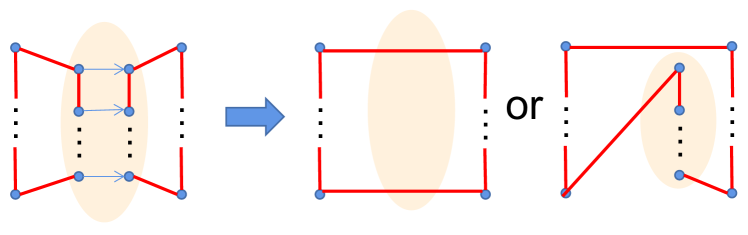
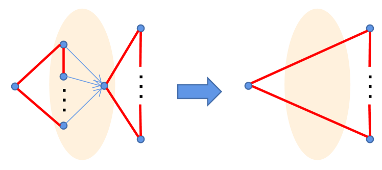
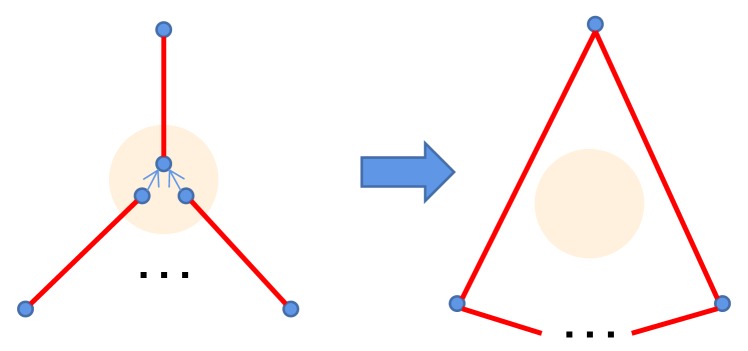
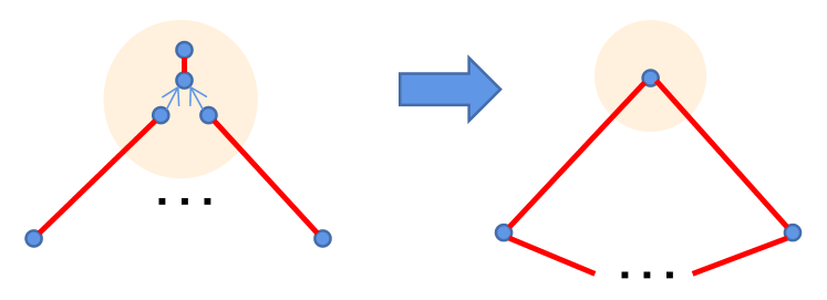
Figure 5: (a)-(b) Schematic diagrams for generation $d$-dimensional multi-particle GHZ states from two multi-particle GHZ states. Red polygons represent $d$-dimensional GHZ states with vertexes being as qudits. Arrows in the yellow area represent quantum walk operations with start points and target points being coin states and position states, respectively. (a) After performing quantum walk and measurement operations, we will generate a GHZ state among qudits outside the yellow area or between qudits outside the yellow area and $k$ qudits in the yellow area. (b) we will generate a GHZ state among qubits outside the yellow area. (c)-(d) Schematic diagrams for generation $d$-dimensional multi-particle GHZ states from multiple d-dimensional Bell states. Red line segments and polygons represent $d$-dimensional Bell states and GHZ states with vertexes being as qudits. Arrows in the yellow area represent quantum walk operations with start points and target points being coin states and position states, respectively. (c) After performing quantum walk and measurement operations, we will generate a GHZ state among qudits outside the yellow area. (d) We prepare a Bell state locally in the yellow area and let a qudit be position state to perform the above quantum walks, then we will generate a GHZ state between qubits outside the yellow area and a qudit in the yellow area.

d-dimensional multi-particles GHZ states

We can also generate a $d$-dimensional multi-particles GHZ state through multiple d-dimensional Bell states and the quantum walk with multiple coins as shown in the Figure 5 and Figure 5. Here we only consider the d-dimensional Bell state $|\psi_{0,0}\rangle=\frac{1}{\sqrt{d}}\sum\limits_{i=0}^{d-1}|i,i\rangle$, since $|\psi_{0,0}\rangle$ can be generated from the generalized d-dimensional Bell state $|\psi_{m,n}\rangle$ by acting on the first qudit with $U_{m,n}=\sum\limits_{i=0}^{d-1}\omega^{-mi}|i-n\rangle\langle i|$. Suppose there are $M+1$ d-dimensional Bell states in the initial state space shown as follow:

$$|\Psi(0)\rangle=\bigotimes\limits_{k=1}^{M}\big{(}\frac{1}{\sqrt{d}}\sum\limits_{i_{k}=0}^{d-1}|i_{k},i_{k}\rangle_{2k-1,2k}\big{)}$$

$$\otimes\frac{1}{\sqrt{d}}\sum\limits_{j=0}^{d-1}|j,j\rangle_{2M+1,2M+2}.$$ (29)

Take the particles $2k,k=1,2,\cdots,M$ as the coin state at the $k-th$ step of the quantum walk, and the particle $2M+1$ as the position state at every step of the walk. Set the coin operator as $C=F$, and the conditional shift operator as $S=\sum\limits_{k,j=0}^{d-1}|k\rangle\langle k|\otimes|j-k\rangle\langle j|$. After performing $M$ steps of the quantum walk, the quantum state becomes

$$|\Psi(M)\rangle=\bigotimes\limits_{k=1}^{M}\big{(}\frac{1}{d}\sum\limits_{i_{k},p_{k}=0}^{d-1}\omega^{i_{k}p_{k}}|i_{k},p_{k}\rangle_{2k-1,2k}\big{)}$$

$$\otimes\frac{1}{\sqrt{d}}\sum\limits_{j=0}^{d-1}|j-\sum\limits_{k=1}^{M}p_{k},j\rangle_{2M+1,2M+2}.$$ (30)

Then, we take a measurement with the basis $\{|\widetilde{k}\rangle:k=0,\cdots,d-1\}$ and $\{|k\rangle:k=0,\cdots,d-1\}$ on the coin states and the position state, respectively, where the measurement results are recorded as $\widetilde{q_{k0}}$ and $u_{0}$. And we perform the quantum Fourier inverse transformation on the particle $2M+2$, thus the rest quantum state is $\frac{1}{\sqrt{d}}\sum\limits_{r=0}^{d-1}\omega^{-ru_{0}}\bigotimes\limits_{k=1}^{M}|r+\widetilde{q_{k0}}\rangle_{2k-1}\otimes|r\rangle_{2M+2}$, which is a general $d$-dimensional multi-particles GHZ state.

4 Entanglement distribution on arbitrary quantum networks

In this section, we will discuss about the multi-particle entangled state distribution in an arbitrary quantum network by the methods mentioned above. In our quantum network, each node can store qubits (or qudits) or perform local operations on them, and each edge represents an entangled state between two nodes. The method of entanglement swapping is employed in the aforementioned quantum repeater, wherein a multi-particle entangled state is distributed among arbitrarily selected nodes through the utilization of basic entangled states within the network and quantum walk operations.

Our aim is to connect the selected nodes in the quantum network through a connected graph with minimal edges, which can be achieved by implementing the Steiner tree algorithm[49]. This approach allows for additional points to be added outside of the given nodes, resulting in a connected graph with minimal overhead. The cost consideration involves determining the number of basic entangled states or edges required to generate a connected graph that connects these selected nodes with minimum edge count - i.e., the Steiner tree.

We only need to consider how to distribute the entangled state among selected nodes in the tree network.The next step involves determining the optimal distribution of the entangled state among a specific subset of nodes in the tree network. Once a node is selected as the root, the remaining nodes can be categorized into different levels based on their distance from the root. It should be noted that all leaf nodes are considered as part of this selected subset. In the Figure 6 we show the process of distributing the entangled state among the root node and the level 2 nodes. For the three adjacent level nodes as shown in the Figure 6, we perform the operation in the Figure 5 between each parent node and its child nodes to obtain a GHZ state in two adjacent level nodes. Each node can generate a GHZ state with its parent node and sibling nodes, and it can also generate a GHZ state with its child nodes as shown in the Figure 6 and Figure 6. Then perform the operations in the Figure 5 on the two GHZ states in each node, and we can get the GHZ states between the next-closest-level nodes as shown in the Figure 6. By repeating the above operations, we can get the GHZ state between nodes at arbitrary levels. We can perform corresponding measurement operations according to whether the node is a selected node, so as to keep or not keep the qubits or qudits in the node. Thus, we can realize the generation of GHZ states between any selected nodes in the tree network.

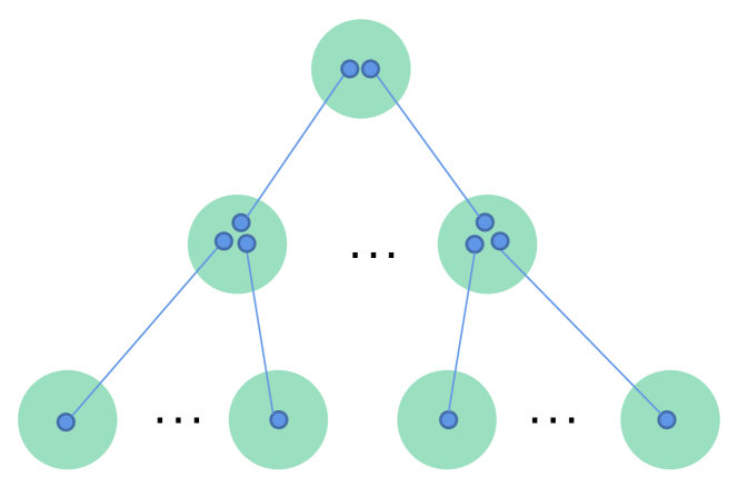
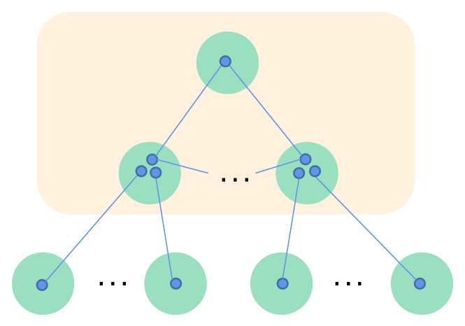
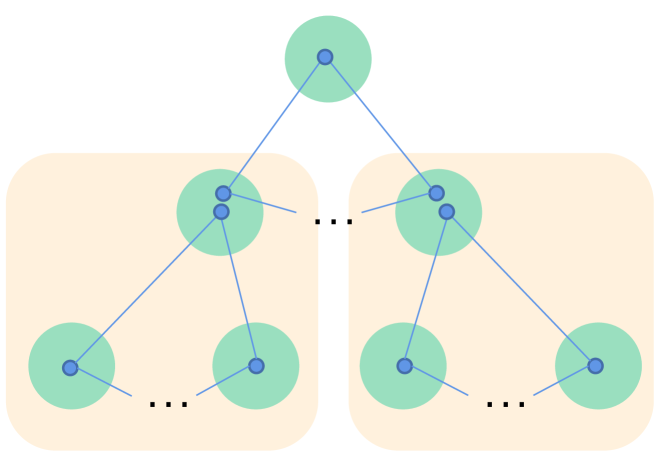
Figure 6: The schematic diagram of distributing a GHZ state between the root node and the level 2 nodes. (a) A tree network with the root node and two level nodes. (b) and (c) We perform quantum walks between each parent node and its child nodes to obtain a GHZ state in yellow areas. (d) We perform quantum walks on the two GHZ states in each middle level node to generate a GHZ state among the root node and the level 2 nodes.

Finally, we give an example of a concrete quantum network with $14$ nodes, and describe the process of distributing GHZ states in several nodes selected in it as shown in the Figure 7. Select nodes 1, 2, 5, 12, 13 and 14 and mark them in green in the network diagram. Then find the Steiner tree connecting them in the network, and mark the additional points in yellow, and the edge of the Steiner tree in red. The remaining points are marked in blue as shown in the Figure 7. For the Steiner tree, we select node 8 as the root node, and perform corresponding quantum walk operations in nodes 6 and 9. Then node 8 and nodes 3 and 9 generate entangled states respectively as shown in the Figure 7, and then perform the corresponding quantum walk operation on node 8, so nodes 3 and 11 generate an entangled state as shown in the Figure 7. Then corresponding quantum walk operations are performed on nodes 3 and 11 respectively, so nodes 1, 2, 3 and 5, and nodes 11, 12, 13 and 14 generate two GHZ states respectively as shown in the Figure 7. Then perform the corresponding quantum walk operation on node 3 ,thus nodes 1, 2, 5 and 11 generate a GHZ state as shown in the Figure 7. Finally distribute a GHZ state among nodes 1, 2, 5, 12, 13 and 14 as shown in the Figure 7 after performing the corresponding quantum walk operation on node 11. Compared with the article[50], the quantum state we can distribute in an arbitrary quantum network is not only a 2-dimensional quantum state, but also a $d$-dimensional GHZ state, which provides more theoretical basis and experimental potential for high-dimensional quantum communication networks.

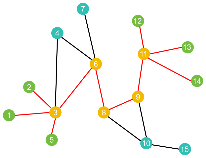
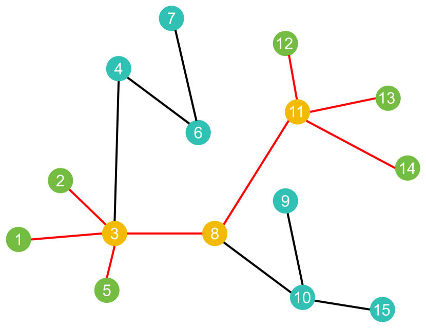
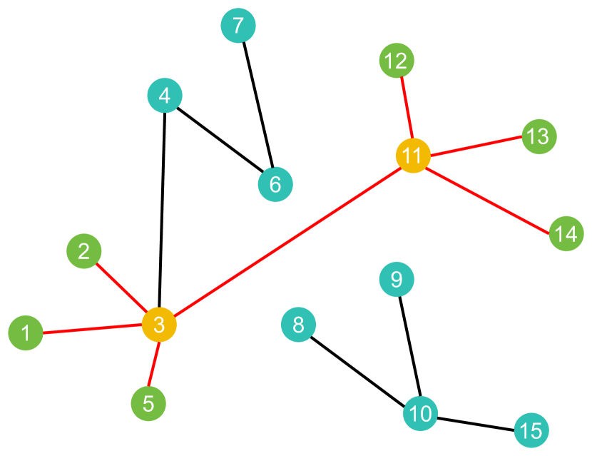
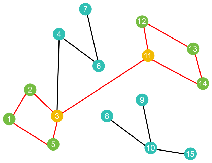
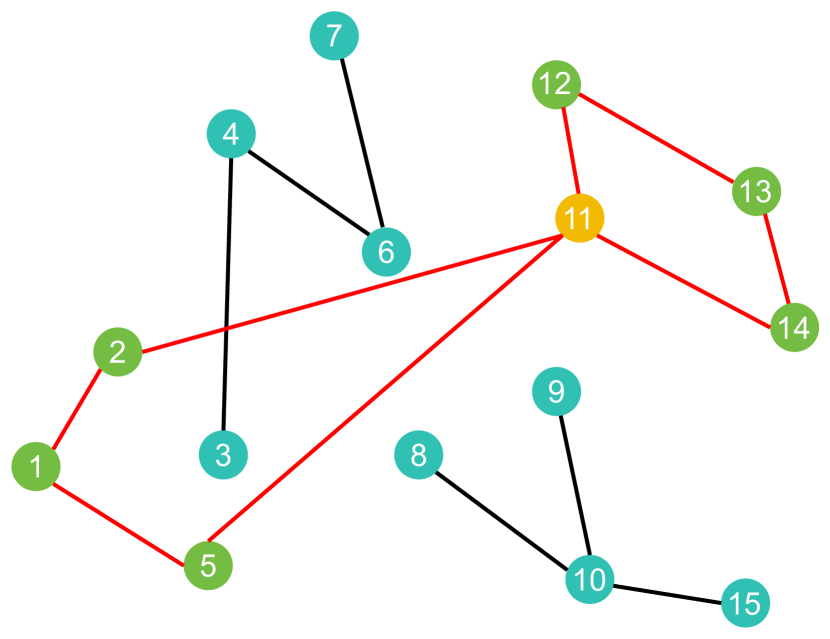
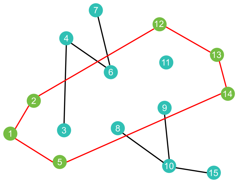
Figure 7: The schematic diagram of distributing a GHZ state among the selected nodes marked in green. (a) The Steiner tree connecting them in the network with red edges. (b)-(f) According to the process of distributing entangled states in the tree network, the corresponding quantum walk and measurement operations are carried out at the corresponding nodes. Finally distribute a GHZ state among nodes 1, 2, 5, 12, 13 and 14.

5 Applications

5.1 Application for constructing quantum fractal networks

We can construct a quantum entanglement fractal network by the above entanglement generation schemes. Inspired by the approach used to create classical complex networks from fractal structures [51, 52], we can extend this methodology to construct a quantum network utilizing the Sierpinski gasket, as depicted in Figures 8(a), 8(b) and 8(c). Each black rectangle represents a quantum node. Each shaded triangle represents a 3-qubit GHZ state, and the three particles of each GHZ state are located in three quantum nodes, forming the structure of the Sierpinski gasket. Let the side length of each small equilateral triangle be $L$, so the side length of $G(N)$, the Sierpinski gasket with N iterations, is $2^{N}L$.

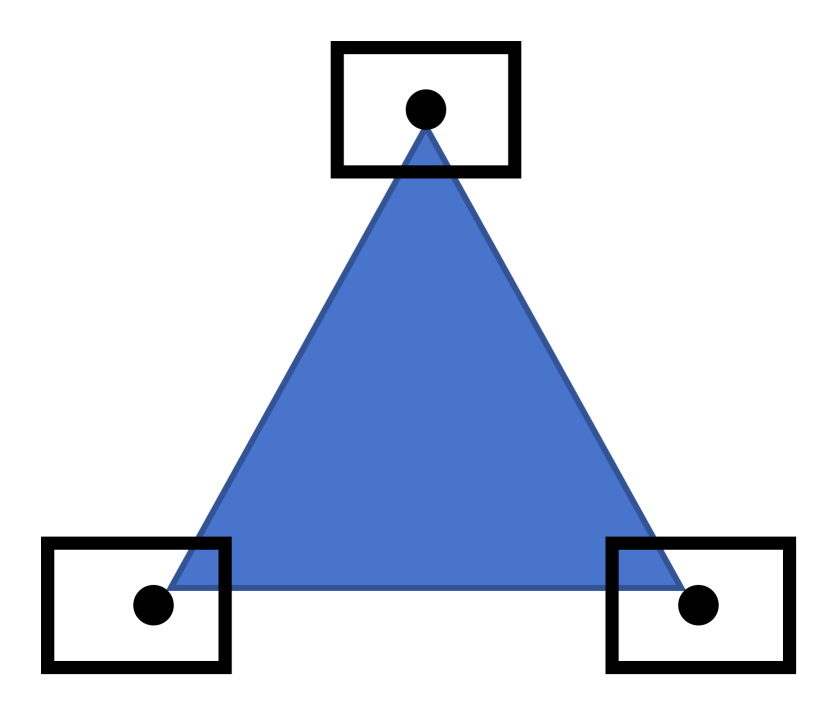
(a) G(0)

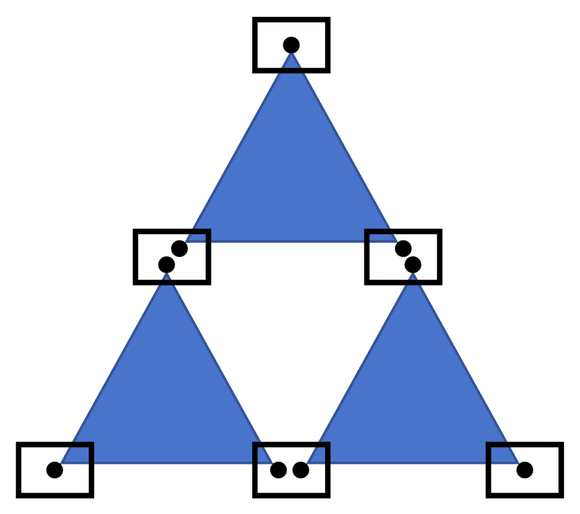
(b) G(1)

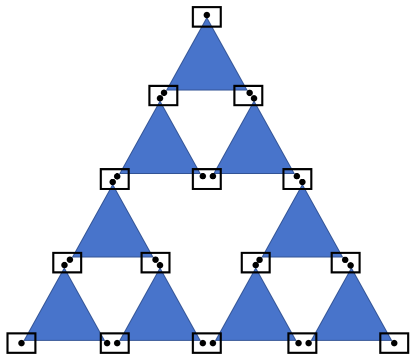
(c) G(2)

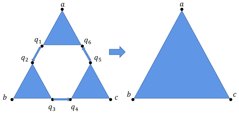
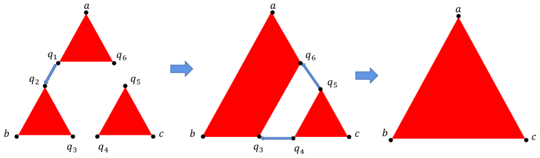
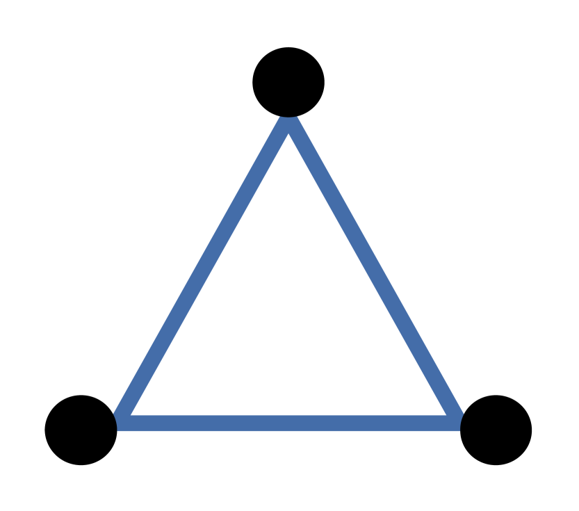
(d) F(0)

(e) F(1)

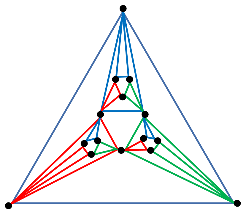
(f) F(2)

Figure 8: (a)-(c) Some Sierpinski gaskets. Each black rectangle represents a quantum node. Each shaded triangle corresponds to a $3$-qubit GHZ state between three quantum nodes. (d) The entanglement swapping of three $3$-qubit GHZ states corresponding to $G(1)$. Every blue shade triangle corresponds to a $3$-qubit GHZ state. And arrow represents a quantum walk operation with starting and target points of arrows representing coin states and position states, respectively. (e) The entanglement swapping of three $3$-qudit GHZ states corresponding to $G(1)$. Every red shade triangle corresponds to a $3$-qudit GHZ state. And arrow represents a quantum walk operation with starting and target points of arrows representing coin states and position states, respectively. (f)-(h) Some evolutionary fractal networks constructed from the Sierpinski gaskets. Black dots represent network nodes. Each triangle represents a three-party channel based on a GHZ entangled state. The triangles in the figure are colored red, green and blue to distinguish different tripartite channels based on different GHZ States.

Unlike the method provided by [53, 54] of using Bell state measurements to connect 3 GHZ states, We can achieve a $3$-qubit GHZ state corresponding to a shade triangle with side length $2L$ from three $3$-qubit GHZ states corresponding to three shade triangle with side length $L$ through the operations in the Figure 8, where an arrow represents a quantum walk operation, and starting and target points of arrows represent coin states and position states, respectively.

We let the initial state in the Figure 8 be

$$|\Psi(0)\rangle= \frac{|000\rangle+|111\rangle}{\sqrt{2}}_{a,q_{1},q_{6}}\otimes\frac{|000\rangle+|111\rangle}{\sqrt{2}}_{q_{2},b,q_{3}}$$ (31)

$$\otimes\frac{|000\rangle+|111\rangle}{\sqrt{2}}_{q_{4},q_{5},c}.$$

After the quantum walks in the Figure 8, $C=X$, and $S$ is the CNOT gate. The quantum state becomes

$$|\Psi(1)\rangle=\frac{1}{2\sqrt{2}}(|111\rangle(|111\rangle|000\rangle+|000\rangle|111\rangle)$$

$$+|010\rangle(|110\rangle|001\rangle+|001\rangle|110\rangle)$$

$$+|100\rangle(|101\rangle|010\rangle+|010\rangle|101\rangle)$$ (32)

$$+|001\rangle(|011\rangle|100\rangle+|100\rangle|011\rangle))_{q_{6},q_{2},q_{4},q_{1},q_{3},q_{5},a,b,c}.$$

Then, we take a measurement with the basis $\{|+\rangle,|-\rangle\}$ in the particle $q_{1},q_{3},q_{5}$ and the basis $\{|0\rangle,|1\rangle\}$ in the particles $q_{2},q_{4},q_{6}$. The entanglement states of the particles $a,b,c$ can be recovered to the state $\frac{|000\rangle+|111\rangle}{\sqrt{2}}$ by some local unitary operations according to the measurement results.

More, our method is not limited to the 2-dimensional case like the method in [53, 54]. We can generalize our method to the d-dimensional case. This not only avoids the experimental technical difficulty of high-dimensional joint Bell state measurement, but also greatly improves the communication efficiency of quantum networks by using high-dimensional GHZ states. Now, the initial state in the Figure 8 is

$$|\Psi(0)\rangle=\frac{1}{\sqrt{d}}\sum\limits_{i_{1}=0}^{d-1}|i_{1},i_{1},i_{1}\rangle_{a,q_{1},q_{6}}$$ (33)

$$\otimes\frac{1}{\sqrt{d}}\sum\limits_{i_{2}=0}^{d-1}|i_{2},i_{2},i_{2}\rangle_{q_{2},b,q_{3}}\otimes\frac{1}{\sqrt{d}}\sum\limits_{i_{3}=0}^{d-1}|i_{3},i_{3},i_{3}\rangle_{q_{4},q_{5},c}.$$

After the first quantum walk in the Figure 8 with the coin operator $C=I$, and the conditional shift operator $S=\sum\limits_{k,j=0}^{d-1}|k\rangle\langle k|\otimes|j-k\rangle\langle j|$. Then, we take a measurement with the basis $\{|\widetilde{k}\rangle:k=0,\cdots,d-1\}$ and $\{|k\rangle:k=0,\cdots,d-1\}$ on the particles $q_{1}$ and $q_{2}$, respectively. If the measurement results of the particles $q_{1}$ is $\widetilde{p_{1}}$. And the measurement results of the particles $q_{2}$ is $u_{1}$, then the entanglement state of leftover particles is

$$|\Psi(1)\rangle=\frac{1}{\sqrt{d}}\sum\limits_{i_{1}=0}^{d-1}\omega^{-i_{1}\widetilde{p_{1}}}|i_{1},i_{1},i_{1}+u_{1},i_{1}+u_{1}\rangle_{a,q_{6},b,q_{3}}$$

$$\otimes\frac{1}{\sqrt{d}}\sum\limits_{i_{3}=0}^{d-1}|i_{3},i_{3},i_{3}\rangle_{q_{4},q_{5},c}.$$ (34)

After the last two quantum walks in the Figure 8 with the coin operator $C=I$, and the conditional shift operator $S=\sum\limits_{k,j=0}^{d-1}|k\rangle\langle k|\otimes|j-k\rangle\langle j|$. Then, we take a measurement with the basis $\{|\widetilde{k}\rangle:k=0,\cdots,d-1\}$ and $\{|k\rangle:k=0,\cdots,d-1\}$ on the particles $q_{4},q_{5}$ and $q_{3},q_{6}$, respectively. If the measurement results of the particles $q_{4},q_{5}$ are $\widetilde{p_{2}},\widetilde{p_{3}}$. And the measurement results of the particles $q_{6},q_{3}$ are $u_{2},u_{3}$, then $u_{1}+u_{2}=u_{3}$. The entanglement state of leftover particles $|\Psi(2)\rangle$ is

$$\sum\limits_{i_{1}=0}^{d-1}\frac{\omega^{-i_{1}(\widetilde{p_{1}}+\widetilde{p_{2}}+\widetilde{p_{3}})+u_{2}(\widetilde{p_{2}}+\widetilde{p_{3}})}}{\sqrt{d}}|i_{1},i_{1}+u_{1},i_{1}-u_{2}\rangle_{a,b,c}.$$ (35)

The entanglement states of the particles $a,b,c$ corresponding to different measurement results can be recovered to the state $\frac{1}{\sqrt{d}}\sum\limits_{i_{1}=0}^{d-1}|i_{1},i_{1},i_{1}\rangle$ by some local unitary operations according to the measurement results.

Furthermore, we can generate a $3$-qubit or $3$-qudit GHZ state corresponding to a shade triangle with side length $2^{N}L$ from the GHZ states corresponding to the shade triangles in $G(N)$ through $\frac{3^{N}-1}{2}$ operations in the Figure 8 or Figure 8. So we can construct a complex quantum network between quantum nodes by implementing entanglement between these quantum nodes through the above operations. Inspired by classical complex networks in the real life generally have self similarity[55], we can construct a quantum complex network according to the structure of the Sierpinski gasket, which will bring some self similarity to the actual quantum network structure.

From $G(N)$, we can construct the corresponding quantum network $F(N)$. The construction rule is as follows: the GHZ entangled states corresponding to the basic shaded triangles in $G(N)$ are regarded as the basic entangled states, and we assume that these basic entangled states can be prepared directly and continuously. And the three nodes where the particles of basic entangled state are located are entangled by the basic entangled state. By using these basic entangled states and the above entanglement swapping operations, we can prepare GHZ states with particles farther apart, so that some nodes that are not originally entangled by the same entangled state can be entangled by the same entangled state. In the network we construct, we can establish a tripartite channel between three nodes can be entangled by the same GHZ entangled state as shown in Figures 8(d), 8(e) and 8(f). As for the constructed quantum network, we describe its classical complex network properties in more detail in the appendix A.

5.2 Application in multiparty quantum secret sharing protocol (MQSS)

We have discussed about the entanglement generation of $d$-dimensional multi-particles GHZ state through multiple d-dimensional Bell states by quantum walks. In fact, our proposed schemes not only generate entangled states for quantum repeaters and so on, but also really work in the other quantum domain. Such as there are a lot of studies about multiparty quantum secret sharing protocol (MQSS), where some MQSS protocols based on GHZ states are proposed. In 2017, a dynamic quantum secret sharing by using a $d$-dimensional GHZ state was proposed by Qin et al[56]. In this protocol, Alice accomplishes quantum secret sharing with Bob_k($k\in\{1,2,\cdots,M\}$), through three main steps:

1. Alice sends $M$ particles of a $M+1$-qudit GHZ state $\frac{1}{\sqrt{d}}\sum\limits_{i=0}^{d-1}|i,i,\cdots,i\rangle$ prepared by her own to the $M$ participants, and each participant holds a particle.

2. Alice measures her own particle in the $X$-basis, and we assume the measurement result is $q_{0}$. Then Alice sets the secret as $S=d-q_{0}$.

3. Each participant measures his particle in the $X$-basis. Assume the measurement result of Bob_k are $q_{k}$, $k\in\{1,2,\cdots,M\}$. By the property of GHZ state, we can know that $q_{1}+q_{2}+\cdots+q_{M}=S$.

So Alice has shared the secret $S$ among the $M$ participants by using a $d$-dimensional GHZ state.

Here we introduce a physical implementation methods of the protocol through the combination of quantum repeaters and multi-coin quantum walks as shown in Figure 9:

1. Construct a trusted quantum repeater between Alice and Bob_k($k\in\{1,2,\cdots,M\}$) to generate some $d$-dimensional detecting Bell states and a Bell state $\frac{1}{\sqrt{d}}\sum\limits_{i_{k}=0}^{d-1}|i_{k},i_{k}\rangle_{2k-1,2k}$ between them. Bob_k and Alice hold particles $2k-1$ and $2k$, respectively.

2. After preparing a number of $d$-dimensional Bell states between the nodes of the secret distributor and the nodes of all participants, the secret distributor and the participants act Fourier operator and inverse Fourier operator on the particles of the selected Bell state,respectively. If the entangled state between the secret distributor and the participant is a Bell state, the entangled state remains unchanged after the above operation, so that the results of both measurements are the same under the same measurement basis. Alice chooses randomly from two mutually unbiased measurement basis: $\{|\widetilde{k}\rangle:k=0,\cdots,d-1\}$ and $\{|k\rangle:k=0,\cdots,d-1\}$. Alice tells Bob_k the basis she has chosen. They measure their own qudits of detecting Bell states by chosen measurement basis, respectively. Then Bob tells Alice his outcomes of his detecting qudits. Alice compares these two outcomes to compute the error rate through comparing the measurement results(For example, if the generalized Bell state pairs that Alice prepares is$|\psi_{0,0}\rangle$, these two measurement outcomes must be identical when the channel is safe). If the error rate exceeds the threshold value, Alice asks the participants to abort the process and starts a new one. Otherwise, Alice-Bob_k quantum channel is safe and returns to step $3$

3. Alice prepare another $d$-dimensional Bell state is noted as $\frac{1}{\sqrt{d}}\sum\limits_{j=0}^{d-1}|j,j\rangle_{2M+1,2M}$, and perform multi-coin quantum walks among particles $2,4,6,\cdots,2M$ and particle $2M+1$ according to our scheme which can generate a $d$-dimensional multi-particles GHZ state through multiple d-dimensional Bell states to general a $M+1$-qudit GHZ state $\frac{1}{\sqrt{d}}\sum\limits_{r=0}^{d-1}\omega^{-ru_{0}}\bigotimes\limits_{k=1}^{M}|r+\widetilde{q_{k0}}\rangle_{2k-1}\otimes|r\rangle_{2M+2}$ between Alice and Bob_k($k\in\{1,2,\cdots,M\}$). If Alice announces the measurement results, Alice and Bob_k($k\in\{1,2,\cdots,M\}$) can transform this state into a GHZ state $\frac{1}{\sqrt{d}}\sum\limits_{r=0}^{d-1}|r,r,\cdots,r,r\rangle_{1,3,\cdots,2M-1,2M+2}$ through local unitary operations, so that they can share the secret according to Qin’s protocol. But if only Alice knows the measurement results $\widetilde{q_{k0}}$, $k\in\{1,2,\cdots,M\}$, Alice also can share a secret $S$ which is independent to measurement results or other information between the $M$ participants according the fourth step as follow.

4. Alice and Bob_k($k\in\{1,2,\cdots,M\}$) measures their particles in the $Z$-basis, and we assume Alice’s measurement result is $r_{0}$, then Alice publishes classical information $p=\frac{1}{M}(S-\sum\limits_{k=1}^{M}\widetilde{q_{k0}}-Mr_{0})$ on a public channel. Since Bob_k’s measurement result is $r_{0}+\widetilde{q_{k0}}$, the part of the secret $S$ which Alice has shared to Bob_k is $p+r_{0}+\widetilde{q_{k0}}$.

5. When restoring the original information, all participants can add up the partial information in all hands to restore the original information, because $Mp+\sum\limits_{k=1}^{M}\widetilde{q_{k0}}+Mr_{0}=S$.

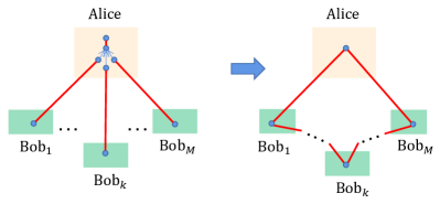
Figure 9: The schematic diagram of our multiparty quantum secret sharing protocol. Red line segments and polygons represent $d$-dimensional Bell states and GHZ states. Arrows in the yellow area represent quantum walk operations with start points and target points being coin states and position states, respectively. Alice prepares some $d$-dimensional Bell states between her and Bob_k($k\in\{1,2,\cdots,M\}$ through quantum repeaters and her one local Bell state. Then by quantum walk and measurement operations, they will generate a $d$-dimensional multi-particle GHZ state $\frac{1}{\sqrt{d}}\sum\limits_{r=0}^{d-1}\omega^{-ru_{0}}\bigotimes\limits_{k=1}^{M}|r+\widetilde{q_{k0}}\rangle_{2k-1}\otimes|r\rangle_{2M+2}$ to share a quantum secret.

The safety of the protocol can be ensured by the step 2 and 4. Step 2 guarantees the security of the communication protocol against both direct measurement attacks, where Eve intercepts and measures the data before resending it to Bob, and intercept and resend attacks, where Eve intercepts the data as it travels between Alice and Bob. Because when the quantum walks and the quantum repeater networks are used for preparing the long-distance entangled state, the particle transmission of the quantum state is avoided, so that the particles which are intercepted and transmitted by other devices when secret information is distributed are avoided. And the strong decoherence of the entangled state in the particle transmission process is also avoided. In security detection, based on the property that a high-dimensional Bell state is invariant under the interaction of two particles with Fourier operator and inverse Fourier operator respectively, the measurement of multiple Bell states can make Alice detect the external entanglement attack of the eavesdropper with high probability. And since the measurement results of the particle $2,4,6,\cdots,2M,2M+2$ are only known by Alice, it is safe to encode the secret information $S$ into the public information $p$. Because $S$ is almost impossible to recover only by $p$. And the original information can be ingeniously transformed and decomposed into the measurement results of each particle in the high-dimensional GHZ state, and no participant can infer the original information from the information in hand, so that the scheme can resist internal attacks.

Compare with Qin’s protocol, our scheme can avoid the sending physical particles process through building quantum repeaters, which can help us defend against some external attacks. And our scheme let Alice can not only share the secret among the $M$ participants through quantum walks and her measurements but also know the secret holds by any participant. More importantly, the information S delivered by Alice is an independent information, which is only decided by Alice at the beginning. Although it is difficult to construct a trusted quantum repeater network with current technological level, our scheme may have certain theoretical advantages. When a trusted quantum repeater network is successfully constructed, it can be reused in quantum communication. Therefore, from a resource perspective, our scheme is much better in theory and has potential application value.

6 Experiments

We have implemented five experiments of generating entangled states by quantum walks on a superconducting quantum computer, which shows the feasibility of our theory in physical experiments to some extent. Superconducting quantum computer we used is Quafu ScQ-P10, and its schematic diagram of the quantum processor is shown in the Figure 10. In these works, the circuits we use consist of 10 qubits in a one-dimensional array. The Hamiltonian of this system is written as follow with the rotating wave approximation

$$H/\hbar=\sum_{i}-\frac{1}{2}\omega_{i}\sigma^{z}_{i}+\sum_{i<j}g_{ij}(\sigma^{+}_{i}\sigma^{-}_{i+1}+h.c.)$$ (36)

where $\omega_{i}$ is the frequency of qubit $Q_{i}$, $g_{ij}$ is the coupling coefficient of qubits $Q_{i},Q_{j}$, and $\sigma^{\pm}$ is the raising (lowering) operator.

Only the nearest-neighbour (NN) qubits are directly coupled through capacitance, with a coupling strength range from 10 to 12 MHz, which is at least one order of magnitude larger than that of non-NN qubits. The two-qubit control-Z gates of NN qubits are achieved within 50 ns with the non-adiabatic scheme adopted, while those of non-NN qubits cannot be achieved due to the coupling strength. The frequency of each qubit can be tuned-up from 4.0 GHz to 5.6 GHz through a microwave line, and excitation can be realized by a microwave drive line for each qubit. All qubits are coupled to one readout line through their individual readout resonators, the frequencies of which are from 6.49 to 6.66 GHz. Readout is achieved through one shared readout line coupled to readout resonators of all qubits. Other information of SCQ see appendix B-D. For each experiment, we show the result with the highest average fidelity among the five repetitions by plotting the density matrix obtained from the experiment in appendix E.

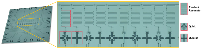
Figure 10: The schematic diagram of quantum processor Quafu ScQ-P10. Ten transmon qubits are integrated on the quantum processor as a one-dimensional chain, and adjacent qubits are directly coupled through capacitance. It shows two types of qubits with different shapes of capacitors, resulting in different sweet spots of approximately 500MHz. In our experiments, each qubit exists as an artificial two-level system.

6.1 Two 2-dimensional Bell states

We generate a new Bell state between $q[0]$ and $q[3]$ from two Bell states as show in the Figure 11. The entire experiment is divided into three stages: preparation, quantum walk and measurement. In the preparation stage, we prepare two Bell state between $q[0],q[1]$ and $q[2],q[3]$, respectively. In the quantum walk stage, we perform corresponding quantum walk between $q[1]$ and $q[2]$ according to the above theory. In the measurement stage, we measure $q[1]$ and $q[2]$ in proper basis and obtain a new Bell state. In the Figure 11, quantum circuit are recompiled into pulse form, and the pulse sequences are sensed by real qubits corresponding to the quantum circuit. On considering the way qubits connected with due to the geometric structure, a two-qubit Control-Z gate can only be formed between adjacent qubits. In our all experiments, the rotation around the z-axis is achieved by virtual Z which has been omitted in the schematic diagrams of pulse sequences for clarity, and single qubit rotation is achieved using microwave pulses with the same frequency as the idle point of the qubit. Two approximately square wave pulses are used to achieve CZ gates between adjacent qubits. The orange line represents the pulse acting on the coin qubit. The gray line represents the pulse acting on the position qubit. The blue line represents the pulse acting on the desired qubits.

In this work, $q[0],q[1],q[2],q[3]$ in quantum circuits are mapped to qubits $Q_{4},Q_{5},Q_{7},Q_{6}$ on the real quantum processor, respectively. According to the Table 1, We can obtain the fidelity of the new generated entangled state between $q[0]$ and $q[3]$ corresponding to any measurement result of $q[1]$ and $q[2]$ through quantum state tomography[57]. We run this experiment with 10000 shots on Quafu ScQ-P10. And the results are shown in the Figure 11. Through these fidelity we can get average fidelity $F=79.8(2.0)\%$

6.2 Two 2-dimensional GHZ states

For the generation of a 2-dimensional GHZ state from a pair of GHZ states, according to the above theory, we have two methods. One is to directly use the 2-dimensional GHZ state generation method, and the other is to use the d-dimensional GHZ state generation method to set $d=2$.

6.2.1 method 1

According to the above entanglement generation scheme of a 2-dimensional GHZ state, we construct a quantum circuit and recompile it into pulse form as shown in the Figure 11, where $q[0],q[1],q[2],q[3],q[4],q[5]$ in quantum circuits are mapped to qubits $Q_{4},Q_{5},Q_{7},Q_{6},Q_{8},Q_{9}$ on the real quantum processor, respectively. The entire experiment is also divided into three stages: preparation , quantum walk and measurement. In the preparation stage, we prepare two GHZ states between $q[0],q[1],q[2]$ and $q[3],q[4],q[5]$, respectively. In the quantum walk stage, we perform corresponding quantum walk between $q[1],q[2]$ and $q[3]$ according to the above theory. In the measurement stage, we measure $q[1],q[2]$ and $q[3]$ in proper basis and obtain a new GHZ state between $q[0],q[4]$ and $q[5]$. We run the quantum circuit with 10000 shots on Quafu ScQ-P10. Through the quantum state tomography, we can obtain the fidelity of the entangled state among $q[0],q[4]$ and $q[5]$ corresponding to any measurement result of $q[1],q[2]$ and $q[3]$ according to the Table 2. The fidelity results are shown in the Figure 11. Through these fidelity we can get average fidelity $F=54.3(3.6)\%$

6.2.2 method 2

According to the above entanglement generation scheme of a $d$-dimensional GHZ state, we can construct a quantum circuit of entanglement generation scheme of a $2$-dimensional GHZ state by setting $d=2$ and recompile it into pulse form as shown in the Figure 11, where $q[0],q[1],q[2],q[3],q[4],q[5]$ in quantum circuits are mapped to qubits $Q_{4},Q_{5},Q_{7},Q_{6},Q_{8},Q_{9}$ on the real quantum processor, respectively. The entire experiment is also divided into three stages: preparation , quantum walk & local recover operator and measurement. In the preparation stage, we prepare two GHZ states between $q[0],q[1],q[2]$ and $q[3],q[4],q[5]$, respectively. In the quantum walk & local recover operator stage, we perform corresponding quantum walk between $q[1],q[2]$ and $q[3]$ according to the above theory and perform a local recover operator on $q[0]$. In the measurement stage, we measure $q[1],q[2]$ and $q[3]$ in proper basis and obtain a new GHZ state between $q[0],q[4]$ and $q[5]$. We run the quantum circuit with 10000 shots on Quafu ScQ-P10. Through the quantum state tomography, we can obtain the fidelity of the entangled state among $q[0],q[4]$ and $q[5]$ corresponding to any measurement result of $q[1],q[2]$ and $q[3]$ according to the Table 5. The fidelity results are shown in the Figure 11. Through these fidelity we can get average fidelity $F=54.3(3.2)\%$

Measurement	Entanglement	Local
results	states	operations
000	$\frac{1}{\sqrt{2}}(|000\rangle+|111\rangle)$	$I_{1}$
001	$\frac{1}{\sqrt{2}}(|011\rangle+|100\rangle)$	$X_{1}$
110	$\frac{1}{\sqrt{2}}(|000\rangle-|111\rangle)$	$Z_{1}$
111	$\frac{1}{\sqrt{2}}(|011\rangle-|100\rangle)$	$X_{1}Z_{1}$

Table 5: Entangled states of $q[0],q[4]$ and $q[5]$. The measurement results of $q[1],q[2]$ and $q[3]$ are shown in the first column. The second column represents the entangled states of $q[0],q[4]$ and $q[5]$ corresponding to different measurement results. The third column represents the local unitary operations on the particle $q[0]$ recovering the state of particles $q[0],q[4]$ and $q[5]$ to $\frac{|000\rangle+|111\rangle}{\sqrt{2}}$.

6.3 Three 2-dim Bell states

According to the above entanglement generation scheme of a GHZ state from multiple Bell states, we can construct a quantum circuit of entanglement generation scheme of a $2$-dimensional GHZ state from three 2-dimensional Bell states and recompile it into pulse form as shown in the Figure 11, where $q[0],q[1],q[2],q[3],q[4],q[5]$ in quantum circuits are mapped to qubits $Q_{5},Q_{8},Q_{7},Q_{9},Q_{6},Q_{4}$ on the real quantum processor, respectively. The entire experiment is also divided into three stages: preparation , quantum walk & local recover operator and measurement. In the preparation stage, we prepare three Bell states between $q[0]$ and $q[1]$ , $q[2]$ and $q[3]$, $q[4]$ and $q[5]$, respectively. In the quantum walk & local recover operator stage, we perform corresponding quantum walk between $q[1],q[2]$ and $q[4]$ according to the above theory and perform a local recover operator on $q[3]$. In the measurement stage, we measure $q[1],q[2]$ and $q[4]$ in proper basis and obtain a new GHZ state between $q[0],q[3]$ and $q[5]$. We run the quantum circuit with 10000 shots on Quafu ScQ-P10. Through the quantum state tomography, we can obtain the fidelity of the entangled state among $q[0],q[3]$ and $q[5]$ corresponding to any measurement result of $q[1],q[2]$ and $q[4]$ according to the Table 6. The fidelity results are shown in the Figure 11. Through these fidelity we can get average fidelity $F=54.4(1.1)\%$

Measurement	Entanglement	Local
results	states	operations
000	$\frac{1}{\sqrt{2}}(|000\rangle+|111\rangle)$	$I_{1}$
001	$\frac{1}{\sqrt{2}}(|001\rangle+|110\rangle)$	$X_{6}$
010	$\frac{1}{\sqrt{2}}(|000\rangle-|111\rangle)$	$Z_{1}$
011	$\frac{1}{\sqrt{2}}(|001\rangle-|110\rangle)$	$Z_{6}X_{6}$
100	$\frac{1}{\sqrt{2}}(|011\rangle+|100\rangle)$	$X_{1}$
101	$\frac{1}{\sqrt{2}}(|010\rangle+|101\rangle)$	$X_{4}$
110	$\frac{1}{\sqrt{2}}(-|011\rangle+|100\rangle)$	$Z_{1}X_{1}$
111	$\frac{1}{\sqrt{2}}(-|010\rangle+|101\rangle)$	$X_{4}Z_{4}$

Table 6: Entangled states of $q[0],q[3]$ and $q[5]$. The measurement results of $q[1],q[2]$ and $q[4]$ are shown in the first column. The second column represents the entangled states of $q[0],q[3]$ and $q[5]$ corresponding to different measurement results. The third column represents the local unitary operations on the particle $q[0]$ recovering the state of particles $q[0],q[3]$ and $q[5]$ to $\frac{|000\rangle+|111\rangle}{\sqrt{2}}$.

6.4 Three 2-dim GHZ states

According to the above entanglement generation scheme of a GHZ state from three GHZ states as shown in the Figure 8, we can construct a quantum circuit of entanglement generation scheme of a $2$-dimensional GHZ state from three GHZ states and recompile it into pulse form as shown in the Figure 11 and Figure 11 where $q[0],q[1],q[2],q[3],q[4],q[5],q[6],q[7],q[8]$ in quantum circuits are mapped to qubits $Q_{1},Q_{2},Q_{3},Q_{4},Q_{6},Q_{5},Q_{7},Q_{8}$ on the real quantum processor, respectively.The entire experiment is also divided into three stages: preparation , quantum walk and measurement. In the preparation stage, we prepare three GHZ states between $q[0],q[1],q[3]$ and $q[2],q[4],q[6]$ and $q[5],q[7],q[8]$ respectively. In the quantum walk stage, we perform corresponding quantum walk between $q[1],q[2],q[3],q[5],q[6]$ and $q[7]$ according to the above theory. In the measurement stage, we measure $q[1],q[2],q[3],q[5],q[6]$ and $q[7]$ in proper basis and obtain a new GHZ state between $q[0],q[4]$ and $q[8]$. We run the quantum circuit with 10000 shots on Quafu ScQ-P10. Through the quantum state tomography, we can obtain the fidelity of the entangled state among $q[0],q[4]$ and $q[8]$ corresponding to any measurement result of $q[1],q[2]$, $q[3],q[5],q[6]$, $q[7]$. The fidelity results are shown in the Figure 11. Through these fidelity we can get average fidelity $F=47.0(0.7)\%$

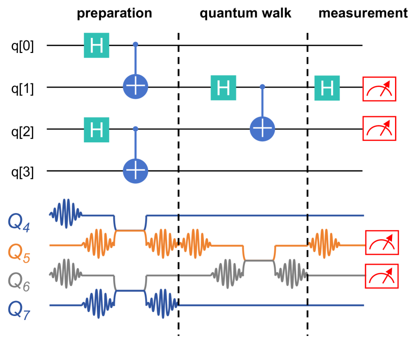
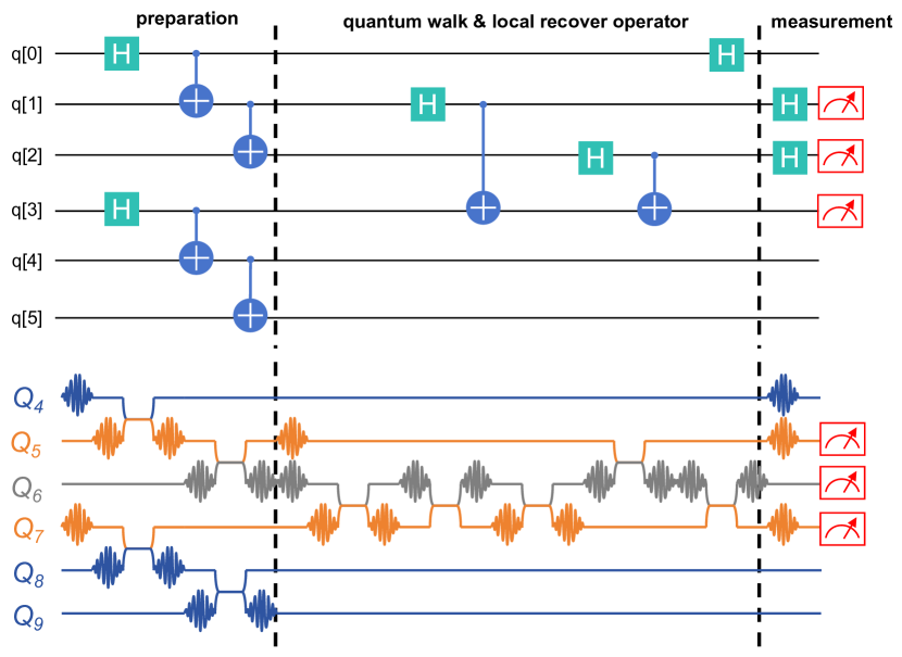
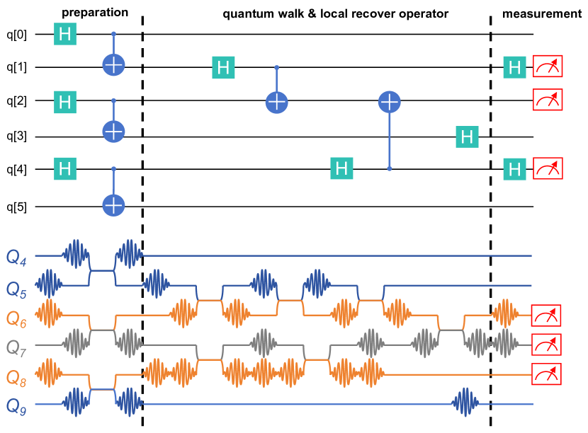
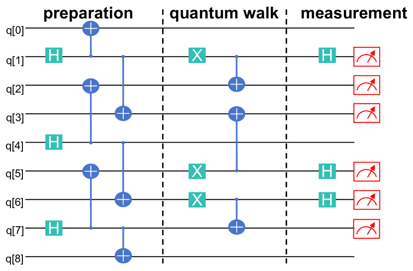
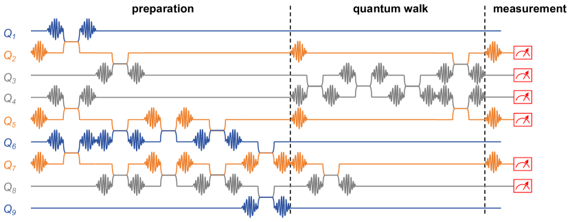
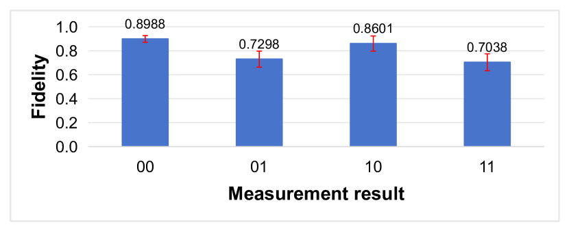
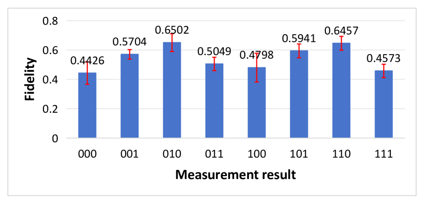
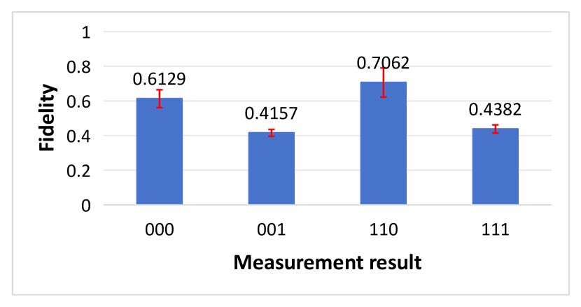
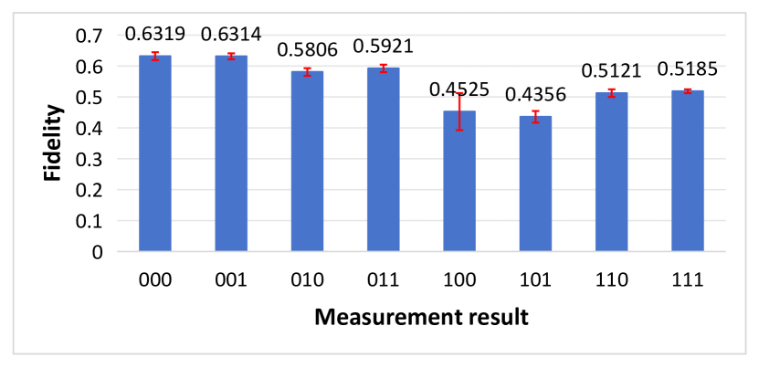
Figure 11: (a) The schematic diagram of the quantum circuit and its pulse form of the entanglement swapping experiment for two 2-dimensional Bell state. (b) The schematic diagram of the quantum circuit and its pulse form of the method 1 for the entanglement swapping experiment of two 2-dimensional GHZ states. (c) The schematic diagram of the quantum circuit and its pulse form of the method 2 for the entanglement swapping experiment of two 2-dimensional GHZ states. (d) The schematic diagram of the quantum circuit and its pulse form of the entanglement swapping experiment of three 2-dimensional Bell states. (e)-(f) The schematic diagram of the quantum circuit and its pulse form of the entanglement swapping experiment of three 2-dimensional GHZ states. (g) The fidelity of the experimental quantum states of $q[0]$ and $q[3]$ corresponding to different measurements of $q[1]$ and $q[2]$ in (a). (h) The fidelity of the experimental quantum states of $q[0],q[4],q[5]$ corresponding to different measurements of $q[1],q[2]$ and $q[3]$ in (b). (i) The fidelity of the experimental quantum states of $q[0],q[4]$ and $q[5]$ corresponding to different measurements of $q[1],q[2]$ and $q[3]$ in (c). (j) The fidelity of the experimental quantum states of $q[0],q[3],q[5]$ corresponding to different measurements of $q[1],q[2]$ and $q[4]$ in (d). (k) The fidelity of the experimental quantum states of $q[0],q[4],q[8]$ corresponding to different measurements of $q[1],q[2]$, $q[3],q[5],q[6]$ and $q[7]$ in (e). Error bars are 1 SD calculated from all fidelity of 5 repetitive experimental runs.

7 Discussion

In scalable quantum networks, it is crucial to distribute multi-particle entangled states among selected nodes, especially for high dimensional entangled states. We develop a scheme for the generation of entangled states based on quantum walks with multi-coin or single-coin, including Bell states, 3-particle and multi-particle GHZ entangled states in 2-dimensional and high-dimensional cases. And we give our high-dimensional entanglement distribution scheme on arbitrary quantum networks according to the above theoretical schemes. We also experimented with the generation of Bell states and three-qubit GHZ states on a quantum computing processor, and obtained high fidelity through quantum state tomography.

Our entanglement generation scheme, in contrast to the article [33], not only circumvent the challenging task of performing joint Bell state measurements and high-dimensional multi-particle GHZ state measurements via quantum walks but also offer a more suitable framework for quantum repeaters in quantum networks. This provides a novel and comparatively straightforward implementation method for constructing larger-scale quantum networks in the future. Compared to the traditional 2-dimensional Bell state-based quantum repeater framework and its experimental realization, our framework enables the utilization of high-dimensional Bell states and GHZ states with any number of particles as fundamental entangled states. This offers additional design possibilities for future large-scale quantum network architecture, as well as a stronger theoretical foundation for combating quantum noise and facilitating efficient communication.

As applications, we give an example of constructing a quantum fractal network based on d-dimensional GHZ states, and analyze some characteristics of its network structure. Furthermore, we propose an enhanced multi-party quantum secret sharing method utilizing our scheme. Following our improvement, it can efficiently generate long-distance high-dimensional entangled states through the framework of quantum repeaters, enabling the secret sender to possess knowledge of the information acquired by each secret receiver, thereby contributing to the management of confidential information. In the future, we will consider to distribute other multi-particle entangled states in arbitrary quantum network nodes, such as Dicke states.

Competing interests

The authors declare no competing interests.

Appendix

Appendix A Properties of Quantum Fractal Network

When we construct a quantum fractal network based on the Sierpinski gasket, a tripartite channel is established between three nodes where the particles of the same GHZ state are located. The way of constructing channels based on entangled states determines some properties of the fractal networks we have constructed. We will analyze these properties from the perspective of complex networks.

After calculation, the number of vertices $N(t)$ in $F(t)$ is $\frac{3^{t+1}+3}{2}$, and the number of edges $E(t)=\frac{3^{t+2}-3}{2}$. Therefore, for a large $t$, the average degree $\overline{k(t)}=\frac{2E(t)}{N(t)}$ is about 6, indicating that this is a sparse network[58] similar to some actual networks.

At $F(t_{i}),t_{i}>0$ , the new vertex $i$ in $F(t)$ has a degree of $k=4(t-t_{i}+1)$. The three nodes in $F(0)$ do not affect the degree distribution of the network when $t$ is large, so they can be ignored. Thus the cumulative degree distribution $P(k)=\frac{3^{t_{i}+1}-3}{3^{t+1}+3}$. Set $t_{i}=t-\frac{k}{4}+1$ and $t$ tends to infinity, then $P(k)=3\cdot e^{-\frac{\ln{3}\cdot k}{4}}$. From this, we can know that the degree distribution of this network meets the exponential distribution, not the power law distribution.

For the vertex $i$ with $k$ in the middle of $F(t)$ above, the number of edges between its adjacent points $e=4+\frac{3}{2}(k-4)$, and $k=4(t-t_{i}+1)$, then the average clustering coefficient $C(t)$ of $F(t)$ is

$$\sum\limits_{t_{i}=1}^{t}\frac{3^{t_{i}}}{3^{t+1}+3}\cdot\frac{4e}{k(k-1)}+\frac{6}{3^{t+1}+3}\cdot\frac{3t+1}{(t+1)(2t+1)}.$$ (37)

When $t$ tends to infinity, $C(t)$ tends to a non-zero constant of 0.5480. Therefore, we can know that the network has small world property[59] through the larger clustering coefficient and the linear relationship between the average path length and the logarithm of the number of vertices, which exist in general actual complex networks.

Appendix B Experimental setup

In this experiment, the quantum processor consists of 10 superconducting qubits, with neighboring qubits coupled through capacitance, and all the qubits are arranged in a one-dimensional chain. The quantum processor worked in low-temperature environment of about 10 mk formed by cryogenic equipment, and each qubit requires one microwave channel to control the frequency of it, and another microwave channel is needed for excitation. A group of control electronics working at room-temperature such as arbitrary waveform generators and microwave sources provide microwave pulses, which are connected to quantum chips through microwave transmission lines. In addition, a microwave channel is also needed to transmit readout pulses, and a microwave transmission line is used to measure states of all qubits simultaneously. The scattered signal is demodulated by ADC to obtain measurement results. The wiring of control electronics and cryogenic equipment are shown in the Figure 12.

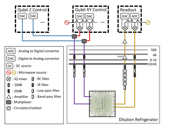
Figure 12: Wiring of cryogenic and control electronics equipment. The QPU is installed at 10 mk stage of the dilution refrigerator. We merge fast Z control line and XY control line of each qubit into one outside the dilution refrigerator. For readout, all qubits can be measured simultaneously.

Due to fixed coupling rates, the difference of idle frequecies between adjacent qubits should be large enough to minimize residual Z-Z coupling between qubits with large detuning, also known as AC Stark effect. When applying readout pulses to each qubit simultaneously, each qubit is biased at a designed point to reduce correlated readout errors caused by measurement.

Some parameters of quantum processor are shown in Table 7 and Table 8. The fidelities of two-qubit CZ gates are obtained by quantum process tomography.The qpt fidelity is obtained when other qubits are on the groud state.

Qubit	$Q_{1}$	$Q_{2}$	$Q_{3}$	$Q_{4}$	$Q_{5}$	$Q_{6}$	$Q_{7}$	$Q_{8}$	$Q_{9}$	$Q_{10}$
$\omega^{s}_{j}/2\pi$ (GHz)	5.536	5.069	5.660	4.742	5.528	4.929	5.451	4.920	5.540	4.960
$\omega_{10,j}/2\pi$ (GHz)	5.310	4.681	5.367	4.702	5.299	4.531	5.255	4.627	5.275	4.687
$\omega^{r}_{j}/2\pi$ (GHz)	5.493	4.800	5.455	4.734	5.300	4.436	5.252	4.807	5.309	4.402
$\eta_{j}/2\pi$ (GHz)	0.250	0.207	0.251	0.206	0.251	0.203	0.252	0.204	0.246	0.208
$g_{j,j+1}/2\pi$ (MHz)	12.07	11.58	10.92	10.84	11.56	10.00	11.74	11.70	11.69	-
$T_{1,j}$ (us)	30.1	17.6	23.2	10.7	33.3	61.0	31.0	33.7	25.6	75.2
$T_{2,j}^{*}$ (us)	2.14	1.17	1.56	2.67	1.89	1.30	2.07	1.50	1.56	2.30
$F_{0,j}$ (%)	98.50	98.45	97.40	98.13	97.47	96.43	96.60	96.37	98.17	98.00
$F_{1,j}$ (%)	94.20	93.97	94.80	94.27	92.03	86.80	93.03	90.97	92.17	88.30

Table 7: Device parameters. $\omega^{s}_{j}$ represents the maximum frequency of $Q_{j}$. $\omega_{10,j}$ corresponds to the idle frequency of $Q_{j}$. $\omega^{r}_{j}$ indicates the resonant frequency of $Q_{j}$ during readout. $\eta_{j}$ shows the anharmonicity of $Q_{j}$. $g_{j,j+1}$ is the coupling strength between nearest-neighbor qubits. $T_{1,j}$ and $T^{*}_{2,j}$ represent the relaxation time and coherence time of $Q_{j}$. $F_{0,j}$ and $F_{1,j}$ are readout fidelities of $Q_{j}$ in $|0\rangle$ and $|1\rangle$, which can be used for readout correction.

	$Q_{1}Q_{2}$	$Q_{2}Q_{3}$	$Q_{3}Q_{4}$	$Q_{4}Q_{5}$	$Q_{5}Q_{6}$	$Q_{6}Q_{7}$	$Q_{7}Q_{8}$	$Q_{8}Q_{9}$	$Q_{9}Q_{10}$
$T_{\mathrm{CZ}}(\mathrm{ns})$	48.9	46.1	40.1	39.0	42.8	41.8	43.6	40.5	41.1
$P_{\mathrm{ref}}$ (%)	97.98	98.45	95.74	96.64	98.29	98.24	97.06	96.13	96.19
$P_{\mathrm{target}}$ (%)	96.02	96.16	95.24	95.30	94.63	95.50	94.04	92.11	94.42
$F_{RB}$ (%)	98.50(1)	98.25(1)	99.61(1)	98.95(1)	97.21(1)	97.91(2)	97.67(1)	96.87(1)	98.62(1)

Table 8: Gate fidelities of CZ gates. $T_{\mathrm{CZ}}$ represents the total duration of the pulse forming CZ gate. $P_{\mathrm{ref}}(P_{\mathrm{target}})$ represents depolarization rate obtained from randomly sampled reference(target) sequences. $F_{RB}$ is the process fidelity of CZ gate obtained from randomized benchmarking.

Appendix C Crosstalk correction

In this experiment, the Z control signal and XY control signal of each quantum bit on the quantum processor are combined into a single signal at room temperature and transmitted to the quantum bit through a transmission line. There is classical electromagnetic crosstalk between the control signals corresponding to each quantum bit, and the magnitude of the Z signal crosstalk increases nonlinearly with the increase of signal application time, where the characteristic time is about 10us, This low-frequency crosstalk is caused by inductive coupling between the loops composed of Z-signals from different channels, which can lead to a temporal correlation in the fidelity of the two bit quantum logic gates used in the experiment. Currently, this crosstalk can be greatly reduced through the use of flip soldering packaging technology. However, in this processor, we need to address the issue of crosstalk from the perspective of measurement and control software. As crosstalk changes over time, we cannot perform linear correction through the traditional use of crosstalk matrices. Instead, we measure the response function of bits to the Z-signal input of all other channels, apply compensation pulses, and mitigate Z-signal crosstalk between channels.

In addition to the classic electromagnetic crosstalk of low-frequency signals such as Z signal, there also exists crosstalk of high-frequency signals such as the XY signal in quantum chips. In the experiment, we use the following method to determine the degree of XY crosstalk. Taking $Q_{1}$ and $Q_{2}$ as example, in the first experiment, we do no operation on $Q_{1}$ and conduct Ramsey testing on $Q_{2}$. In the second experiment, as a control, we excite $Q_{1}$ from $|0\rangle$ to $|1\rangle$ through XY signal, and then conduct Ramsey testing on $Q_{2}$. When the periods of two Ramsey curves are equal but the phases are not, it indicates the existence of classical electromagnetic crosstalk in the XY signal, and the magnitude of the phase difference indicates the strength of crosstalk. In this case, we increase the length of XY pulse for pulsing $Q_{1}$ and decrease ulse amplitude to reduce classical XY crosstalk.

Appendix D Readout correction

Due to the interaction between microwave pulses used for dispersion reading and quantum bits, the scattered reading pulses detected by DAC often cannot accurately reflect the state of quantum bits. However, we can correct this part of the errors introduced by reading through post-processing. Firstly, we ensure that there is no correlation between read errors by changing the frequency of the qubits when applying a read pulse. Then, we measure the probability of each quantum bit being in the $|0\rangle$ state, and write it as $F_{0}^{i}$; Then we measure the probability that the result obtained when each quantum bit is in a $|1\rangle$ state is written as $F_{1}^{i}$, which is called read fidelity.

After the above operations, we can obtain the measurement transfer matrix $M_{i}$ for the i-th quantum bit $Q_{i}$,

$$M_{j}=\left(\begin{matrix}F^{j}_{0}&1-F^{j}_{1}\\ 1-F^{j}_{1}&F^{j}_{1}\end{matrix}\right)$$ (38)

which represents the mapping relationship between the ideal measurement result of a single quantum bit and the actual measurement result.

The measurement transfer matrix for multiple quantum bits can be written in the following form:

$$M=M_{0}\otimes M_{1}\otimes\cdots\otimes M_{N},$$ (39)

Therefore, we can eliminate errors introduced by reading by inverting the measurement transfer matrix of multiple qubits, and if the measured probability of the qubit string before correction is $\tilde{\textbf{P}}$, the ideal probability vector obtained from the measurement is

$${\textbf{P}}=M^{-1}\tilde{\textbf{P}}.$$ (40)

Appendix E Schematic diagram of experimental results

For each of the five experiments in the main text, we repeated each experiment five times. In this section, for each experiment, we show the result with the highest average fidelity among the five repetitions by plotting the density matrix obtained from the experiment. The Figure 13-Figure 17 correspond to two Bell state experiments, the method 1 of two GHZ state experiments, method 2 of two GHZ state experiments, three Bell state experiments and three GHZ experiments respectively.

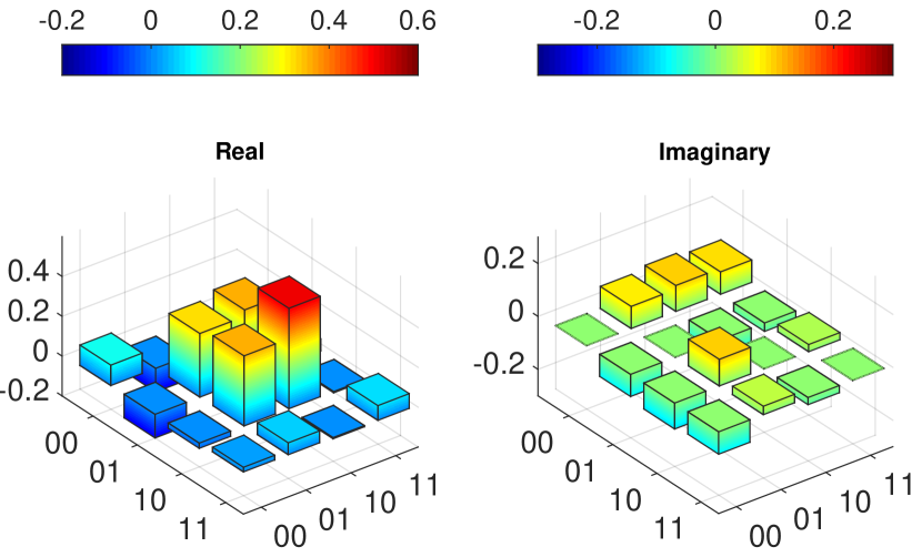
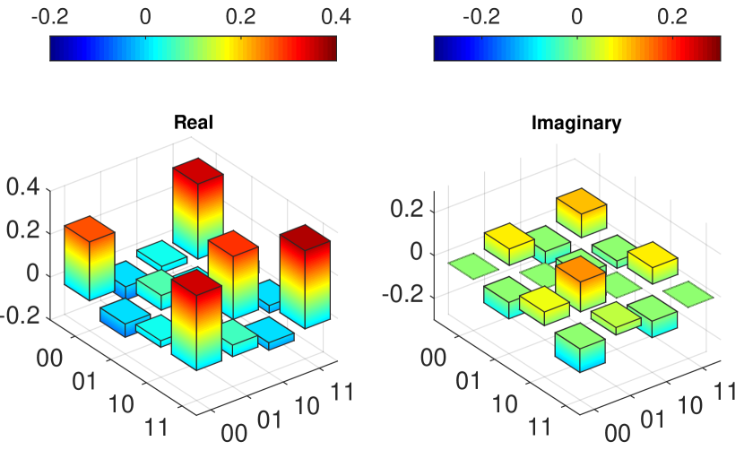
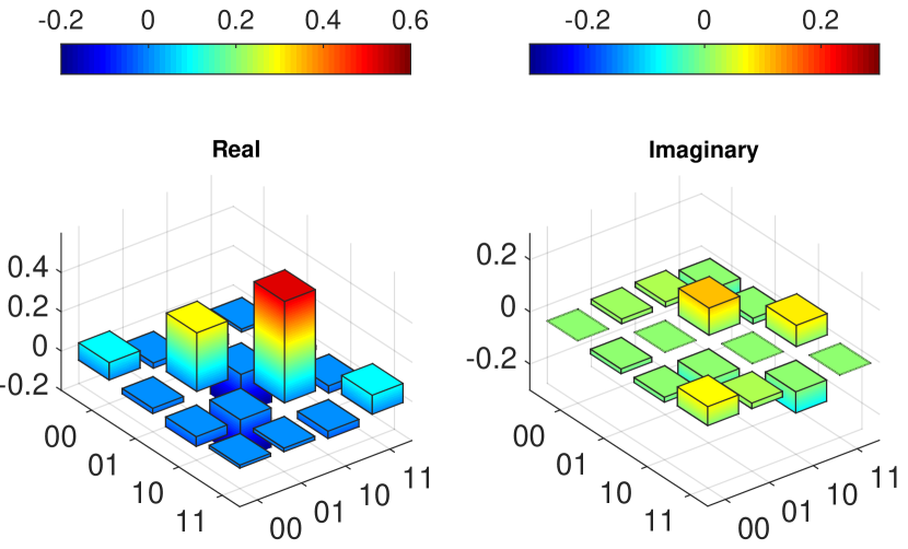
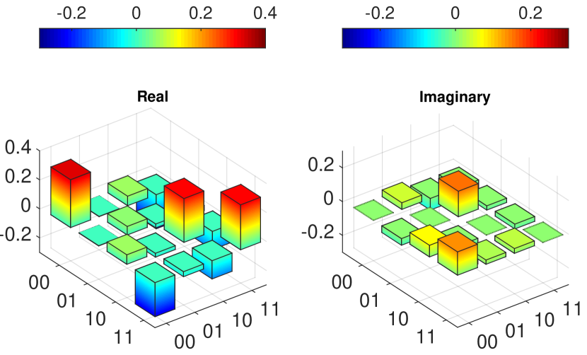
Figure 13: The schematic diagrams of the entanglement density matrices for two 2-dimensional Bell states. The density matrix for each sub-figure corresponds to a different measurement results, with the left figure showing the real part of the density matrix and the right figure showing the imaginary part. The order of the measurement results is consistent with the x-axis in Figure 11(g).

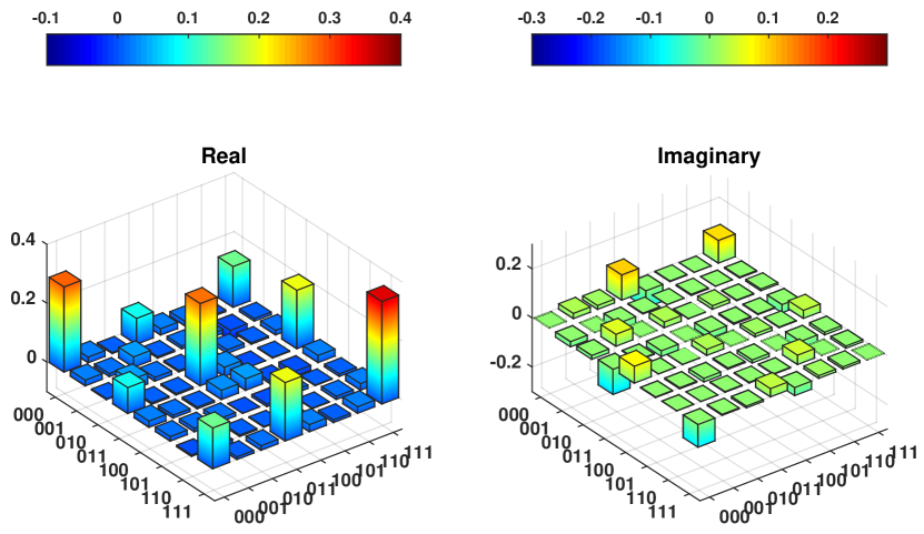
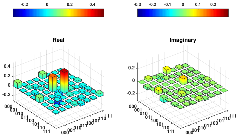
Figure 14: The schematic diagrams of the entanglement density matrices for the method 1 for the entanglement swapping experiment of two 2-dimensional GHZ states. The density matrix for each sub-figure corresponds to a different measurement results, with the left figure showing the real part of the density matrix and the right figure showing the imaginary part. The order of the measurement results is consistent with the x-axis in Figure 11(h).

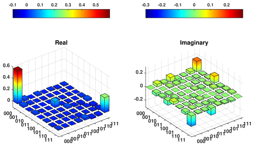
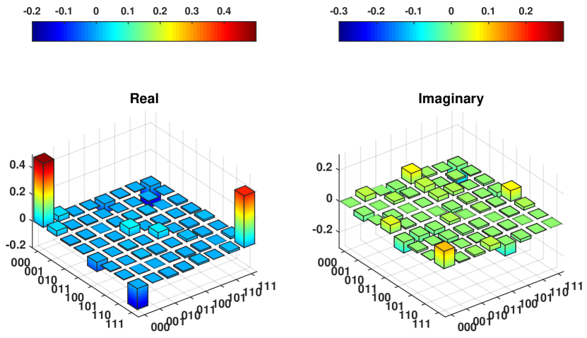
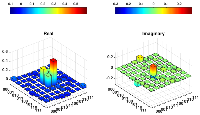
Figure 15: The schematic diagrams of the entanglement density matrices for the method 2 for the entanglement swapping experiment of two 2-dimensional GHZ states. The density matrix for each sub-figure corresponds to a different measurement results, with the left figure showing the real part of the density matrix and the right figure showing the imaginary part. The order of the measurement results is consistent with the x-axis in Figure 11(i).

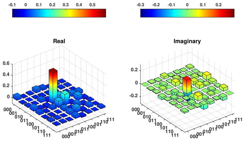
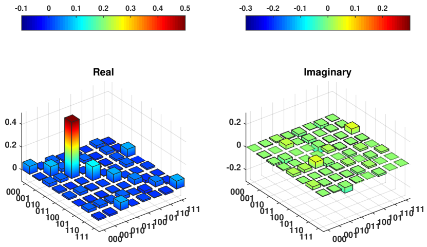
Figure 16: The schematic diagrams of the entanglement density matrices for three 2-dimensional Bell states. The density matrix for each sub-figure corresponds to a different measurement results, with the left figure showing the real part of the density matrix and the right figure showing the imaginary part. The order of the measurement results is consistent with the x-axis in Figure 11(j).

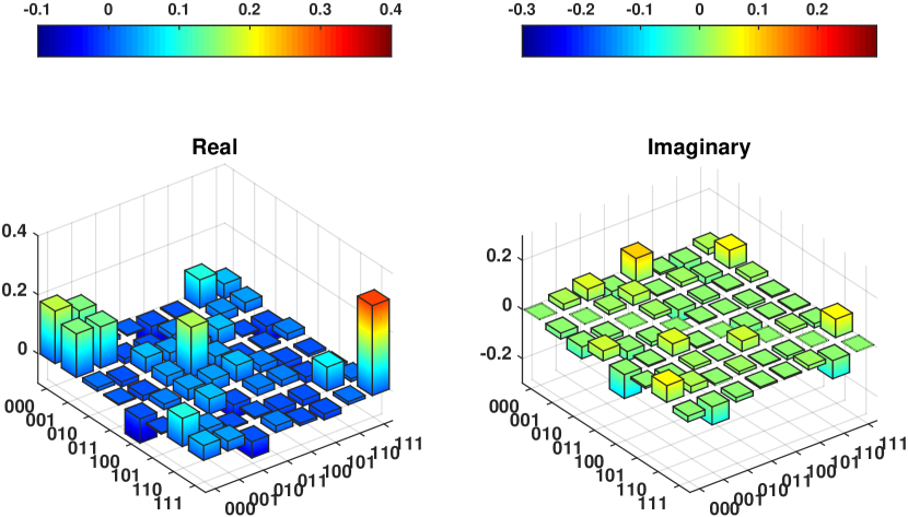
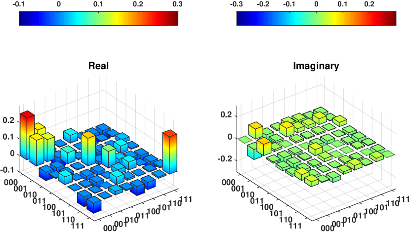
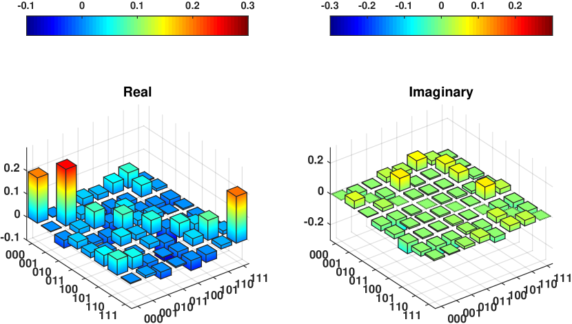
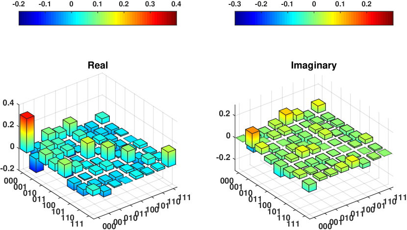
Figure 17: The schematic diagrams of the entanglement density matrices for three 2-dimensional GHZ states. The density matrix for each sub-figure corresponds to a different measurement results, with the left figure showing the real part of the density matrix and the right figure showing the imaginary part. The order of the measurement results is consistent with the x-axis in Figure 11(k).

References

- [1] Y.-A. Chen, Q. Zhang, T.-Y. Chen, W.-Q. Cai, S.-K. Liao, J. Zhang, K. Chen, J. Yin, J.-G. Ren, Z. Chen, et al., An integrated space-to-ground quantum communication network over 4,600 kilometres, Nature 589 (7841) (2021) 214–219.
- [2] D. Cuomo, M. Caleffi, A. S. Cacciapuoti, Towards a distributed quantum computing ecosystem, IET Quantum Communication 1 (1) (2020) 3–8.
- [3] W. Ge, K. Jacobs, Z. Eldredge, A. V. Gorshkov, M. Foss-Feig, Distributed quantum metrology with linear networks and separable inputs, Physical review letters 121 (4) (2018) 043604.
- [4] H. J. Kimble, The quantum internet, Nature 453 (7198) (2008) 1023–1030.
- [5] R. Horodecki, P. Horodecki, M. Horodecki, K. Horodecki, Quantum entanglement, Reviews of modern physics 81 (2) (2009) 865.
- [6] A. K. Ekert, Quantum cryptography based on bell’s theorem, Physical review letters 67 (6) (1991) 661.
- [7] C. H. Bennett, G. Brassard, C. Crépeau, R. Jozsa, A. Peres, W. K. Wootters, Teleporting an unknown quantum state via dual classical and einstein-podolsky-rosen channels, Physical review letters 70 (13) (1993) 1895.
- [8] V. Giovannetti, S. Lloyd, L. Maccone, Quantum metrology, Physical review letters 96 (1) (2006) 010401.
- [9] C. L. Degen, F. Reinhard, P. Cappellaro, Quantum sensing, Reviews of modern physics 89 (3) (2017) 035002.
- [10] H.-J. Briegel, W. Dür, J. I. Cirac, P. Zoller, Quantum repeaters: The role of imperfect local operations in quantum communication, Phys. Rev. Lett. 81 (1998) 5932–5935.
- [11] W. Dür, H.-J. Briegel, J. I. Cirac, P. Zoller, Quantum repeaters based on entanglement purification, Phys. Rev. A 59 (1999) 169–181.
- [12] N. Sangouard, C. Simon, H. de Riedmatten, N. Gisin, Quantum repeaters based on atomic ensembles and linear optics, Rev. Mod. Phys. 83 (2011) 33–80.
- [13] M. Zukowski, A. Zeilinger, M. Horne, A. Ekert, Bell experiment via entanglement swapping, Phys. Rev. Lett 71 (1993) 4287.
- [14] L.-M. Duan, M. D. Lukin, J. I. Cirac, P. Zoller, Long-distance quantum communication with atomic ensembles and linear optics, Nature 414 (6862) (2001) 413–418.
- [15] Z.-D. Li, R. Zhang, X.-F. Yin, L.-Z. Liu, Y. Hu, Y.-Q. Fang, Y.-Y. Fei, X. Jiang, J. Zhang, L. Li, et al., Experimental quantum repeater without quantum memory, Nature photonics 13 (9) (2019) 644–648.
- [16] K. Hammerer, A. S. Sørensen, E. S. Polzik, Quantum interface between light and atomic ensembles, Reviews of Modern Physics 82 (2) (2010) 1041.
- [17] D. L. Moehring, P. Maunz, S. Olmschenk, K. C. Younge, D. N. Matsukevich, L.-M. Duan, C. Monroe, Entanglement of single-atom quantum bits at a distance, Nature 449 (7158) (2007) 68–71.
- [18] J. Hofmann, M. Krug, N. Ortegel, L. Gérard, M. Weber, W. Rosenfeld, H. Weinfurter, Heralded entanglement between widely separated atoms, Science 337 (6090) (2012) 72–75.
- [19] H. Bernien, B. Hensen, W. Pfaff, G. Koolstra, M. S. Blok, L. Robledo, T. H. Taminiau, M. Markham, D. J. Twitchen, L. Childress, et al., Heralded entanglement between solid-state qubits separated by three metres, Nature 497 (7447) (2013) 86–90.
- [20] L. Slodička, G. Hétet, N. Röck, P. Schindler, M. Hennrich, R. Blatt, Atom-atom entanglement by single-photon detection, Physical review letters 110 (8) (2013) 083603.
- [21] L. Stephenson, D. Nadlinger, B. Nichol, S. An, P. Drmota, T. Ballance, K. Thirumalai, J. Goodwin, D. Lucas, C. Ballance, High-rate, high-fidelity entanglement of qubits across an elementary quantum network, Physical review letters 124 (11) (2020) 110501.
- [22] Z. Zeng, Proposal for the complete high-dimensional greenberger–horne–zeilinger state measurement, Laser Physics Letters 20 (9) (2023) 095208.
- [23] Y.-F. Pu, S. Zhang, Y.-K. Wu, N. Jiang, W. Chang, C. Li, L.-M. Duan, Experimental demonstration of memory-enhanced scaling for entanglement connection of quantum repeater segments, Nature Photonics 15 (5) (2021) 374–378.
- [24] N. J. Cerf, M. Bourennane, A. Karlsson, N. Gisin, Security of quantum key distribution using d-level systems, Physical review letters 88 (12) (2002) 127902.
- [25] I. Ali-Khan, C. J. Broadbent, J. C. Howell, Large-alphabet quantum key distribution using energy-time entangled bipartite states, Physical review letters 98 (6) (2007) 060503.
- [26] D. Collins, N. Gisin, N. Linden, S. Massar, S. Popescu, Bell inequalities for arbitrarily high-dimensional systems, Physical review letters 88 (4) (2002) 040404.
- [27] M. Neeley, M. Ansmann, R. C. Bialczak, M. Hofheinz, E. Lucero, A. D. O’Connell, D. Sank, H. Wang, J. Wenner, A. N. Cleland, et al., Emulation of a quantum spin with a superconducting phase qudit, Science 325 (5941) (2009) 722–725.
- [28] B. P. Lanyon, M. Barbieri, M. P. Almeida, T. Jennewein, T. C. Ralph, K. J. Resch, G. J. Pryde, J. L. O’brien, A. Gilchrist, A. G. White, Simplifying quantum logic using higher-dimensional hilbert spaces, Nature Physics 5 (2) (2009) 134–140.
- [29] Y. Aharonov, L. Davidovich, N. Zagury, Quantum random walks, Physical Review A 48 (2) (1993) 1687.
- [30] J. Kempe, Quantum random walks: an introductory overview, Contemporary Physics 44 (4) (2003) 307–327.
- [31] S. E. Venegas-Andraca, Quantum walks: a comprehensive review, Quantum Information Processing 11 (5) (2012) 1015–1106.
- [32] Y. Wang, Y. Shang, P. Xue, Generalized teleportation by quantum walks, Quantum Information Processing 16 (2017) 1–13.
- [33] M. Li, Y. Shang, Entangled state generation via quantum walks with multiple coins, npj Quantum Information 7 (1) (2021) 70.
- [34] A. M. Childs, Universal computation by quantum walk, Physical review letters 102 (18) (2009) 180501.
- [35] N. B. Lovett, S. Cooper, M. Everitt, M. Trevers, V. Kendon, Universal quantum computation using the discrete-time quantum walk, Physical Review A 81 (4) (2010) 042330.
- [36] B. C. Travaglione, G. J. Milburn, Implementing the quantum random walk, Physical Review A 65 (3) (2002) 032310.
- [37] R. Matjeschk, C. Schneider, M. Enderlein, T. Huber, H. Schmitz, J. Glueckert, T. Schaetz, Experimental simulation and limitations of quantum walks with trapped ions, New Journal of Physics 14 (3) (2012) 035012.
- [38] C. A. Ryan, M. Laforest, J.-C. Boileau, R. Laflamme, Experimental implementation of a discrete-time quantum random walk on an nmr quantum-information processor, Physical Review A 72 (6) (2005) 062317.
- [39] A. Schreiber, K. Cassemiro, V. Potoček, A. Gábris, I. Jex, C. Silberhorn, Decoherence and disorder in quantum walks: from ballistic spread to localization, Physical review letters 106 (18) (2011) 180403.
- [40] F. Di Colandrea, A. Babazadeh, A. Dauphin, P. Massignan, L. Marrucci, F. Cardano, Ultra-long quantum walks via spin–orbit photonics, Optica 10 (3) (2023) 324–331.
- [41] M. Karski, L. Förster, J.-M. Choi, A. Steffen, W. Alt, D. Meschede, A. Widera, Quantum walk in position space with single optically trapped atoms, Science 325 (5937) (2009) 174–177.
- [42] S. Dadras, A. Gresch, C. Groiseau, S. Wimberger, G. S. Summy, Quantum walk in momentum space with a bose-einstein condensate, Physical review letters 121 (7) (2018) 070402.
- [43] D. Xie, T.-S. Deng, T. Xiao, W. Gou, T. Chen, W. Yi, B. Yan, Topological quantum walks in momentum space with a bose-einstein condensate, Physical Review Letters 124 (5) (2020) 050502.
- [44] P. Xue, B. C. Sanders, Quantum quincunx for walk on circles in phase space with indirect coin flip, New Journal of Physics 10 (5) (2008) 053025.
- [45] M. Gong, S. Wang, C. Zha, M.-C. Chen, H.-L. Huang, Y. Wu, Q. Zhu, Y. Zhao, S. Li, S. Guo, et al., Quantum walks on a programmable two-dimensional 62-qubit superconducting processor, Science 372 (6545) (2021) 948–952.
- [46] M. G. de Andrade, W. Dai, S. Guha, D. Towsley, A quantum walk control plane for distributed quantum computing in quantum networks, in: 2021 IEEE International Conference on Quantum Computing and Engineering (QCE), IEEE, 2021, pp. 313–323.
- [47] T. A. Brun, H. A. Carteret, A. Ambainis, Quantum walks driven by many coins, Physical Review A 67 (5) (2003) 052317.
- [48] C. Simon, J. Kempe, Robustness of multiparty entanglement, Physical Review A 65 (5) (2002) 052327.
- [49] F. K. Hwang, D. S. Richards, Steiner tree problems, Networks 22 (1) (1992) 55–89.
- [50] C. Meignant, D. Markham, F. Grosshans, Distributing graph states over arbitrary quantum networks, Physical Review A 100 (5) (2019) 052333.
- [51] C. Song, S. Havlin, H. A. Makse, Origins of fractality in the growth of complex networks, Nature physics 2 (4) (2006) 275–281.
- [52] T. Wen, K. H. Cheong, The fractal dimension of complex networks: A review, Information Fusion 73 (2021) 87–102.
- [53] J. Wallnöfer, M. Zwerger, C. Muschik, N. Sangouard, W. Dür, Two-dimensional quantum repeaters, Physical Review A 94 (5) (2016) 052307.
- [54] V. Kuzmin, D. Vasilyev, N. Sangouard, W. Dür, C. Muschik, Scalable repeater architectures for multi-party states, npj Quantum Information 5 (1) (2019) 115.
- [55] C. Song, S. Havlin, H. A. Makse, Self-similarity of complex networks, Nature 433 (7024) (2005) 392–395.
- [56] H. Qin, Y. Dai, Dynamic quantum secret sharing by using d-dimensional ghz state, Quantum information processing 16 (2017) 1–13.
- [57] D. F. James, P. G. Kwiat, W. J. Munro, A. G. White, Measurement of qubits, Physical Review A 64 (5) (2001) 052312.
- [58] S. Luccioli, S. Olmi, A. Politi, A. Torcini, Collective dynamics in sparse networks, Physical review letters 109 (13) (2012) 138103.
- [59] D. J. Watts, S. H. Strogatz, Collective dynamics of ‘small-world’networks, nature 393 (6684) (1998) 440–442.