Robust Decision Transformer: Tackling Data Corruption in Offline RL via Sequence Modeling

Abstract

Learning policies from offline datasets through offline reinforcement learning (RL) holds promise for scaling data-driven decision-making and avoiding unsafe and costly online interactions. However, real-world data collected from sensors or humans often contains noise and errors, posing a significant challenge for existing offline RL methods. Our study indicates that traditional offline RL methods based on temporal difference learning tend to underperform Decision Transformer (DT) under data corruption, especially when the amount of data is limited. This suggests the potential of sequential modeling for tackling data corruption in offline RL. To further unleash the potential of sequence modeling methods, we propose Robust Decision Transformer (RDT) by incorporating several robust techniques. Specifically, we introduce Gaussian weighted learning and iterative data correction to reduce the effect of corrupted data. Additionally, we leverage embedding dropout to enhance the model’s resistance to erroneous inputs. Extensive experiments on MoJoCo, KitChen, and Adroit tasks demonstrate RDT’s superior performance under diverse data corruption compared to previous methods. Moreover, RDT exhibits remarkable robustness in a challenging setting that combines training-time data corruption with testing-time observation perturbations. These results highlight the potential of robust sequence modeling for learning from noisy or corrupted offline datasets, thereby promoting the reliable application of offline RL in real-world tasks.

1 Introduction

Offline reinforcement learning (RL) aims to derive near-optimal policies from fully offline datasets (Levine et al.,, 2020; Wang et al.,, 2018; Fujimoto et al.,, 2019; Kumar et al.,, 2020), thereby reducing the need for costly and potentially unsafe online interactions with the environment. However, offline RL encounters a significant challenge known as distribution shift (Levine et al.,, 2020), which can lead to performance degradation. To address this challenge, several offline RL algorithms impose policy constraints (Wang et al.,, 2018; Fujimoto et al.,, 2019; Fujimoto and Gu,, 2021; Kostrikov et al.,, 2021; Park et al.,, 2024) or maintain pessimistic values for out-of-distribution (OOD) actions (Kumar et al.,, 2020; An et al.,, 2021; Bai et al.,, 2022; Yang et al., 2022a, ; Ghasemipour et al.,, 2022), ensuring that the learned policy aligns closely with the training distribution. Although the majority of traditional offline RL methods rely on temporal difference learning, an alternative promising paradigm for offline RL emerges in the form of sequence modeling (Chen et al.,, 2021; Janner et al.,, 2021; Furuta et al.,, 2021; Shi et al.,, 2023; Wu et al.,, 2024). Unlike traditional RL methods, Decision Transformer (DT) (Chen et al.,, 2021), a representative sequence modeling method, treats RL as a supervised learning task, predicting actions directly from sequences of reward-to-gos, states, and actions. Prior work (Bhargava et al.,, 2023) suggests that DT excels at handling tasks with sparse rewards and suboptimal quality data, showcasing the potential of sequence modeling for real-world applications.

When deploying offline RL in practical settings, dealing with noisy or corrupted data resulting from data collection or malicious attacks is inevitable (Zhang et al.,, 2020; Liang et al.,, 2024; Yang et al., 2024a, ). Therefore, robustly learning policies from such data becomes crucial for the deployment of offline RL. A series of prior works (Zhang et al.,, 2022; Ye et al., 2024b, ; Wu et al.,, 2022; Chen et al.,, 2024; Ye et al., 2024a, ) focus on the theoretical properties and certification of offline RL under data corruption. Notably, a recent study by Ye et al., 2024b proposes an uncertainty-weighted offline RL algorithm with Q ensembles to address reward and dynamics corruption, while Yang et al., 2024b enhance the robustness of Implicit Q-Learning (IQL) (Kostrikov et al.,, 2021) against corruptions on all elements using Huber loss and quantile Q estimators. These advancements, predominantly based on temporal difference learning without utilizing sequence modeling methods, prompt the intriguing question: Can sequential modeling method effectively handle data corruption in offline RL?

In this study, we conduct a comparative analysis of DT with traditional offline RL methods under different data corruption settings. Surprisingly, we observe that traditional methods relying on temporal difference learning struggle in limited data settings and notably underperform DT. Moreover, DT outperforms prior methods under state attack scenarios. These observations highlight the promising potential of sequential modeling for addressing data corruption challenges in offline RL. To further unlock the capabilities of sequential modeling methods under data corruption, we propose a novel algorithm called Robust Decision Transformer (RDT). RDT incorporates three robust techniques for DT, including Gaussian weighted learning, iterative data correction, and embedding dropout to mitigate the impact of corrupted data.

Through comprehensive experiments conducted on a diverse set of tasks, including MoJoCo, KitChen, and Adroit, we demonstrate that RDT outperforms conventional temporal difference learning and sequence modeling approaches under both random and adversarial data corruption scenarios. Additionally, RDT exhibits remarkable robustness in a challenging setting that combines training-time data corruption with testing-time observation perturbations. Our study emphasizes the significance of robust sequential modeling and offers valuable insights that would contribute to the trustworthy deployment of offline RL in real-world applications.

2 Preliminaries

2.1 RL and Offline RL

RL is generally formulated as a Markov Decision Process (MDP) defined by a tuple $(S,A,P,r,\gamma)$. This tuple comprises a state space $S$, an action space $A$, a transition function $P$, a reward function $r$, and a discount factor $\gamma\in[0,1)$. The objective of RL is to learn a policy $\pi(a|s)$ that maximizes the expected cumulative return:

$$\max_{\pi}\mathbb{E}_{s_{0}\sim\rho_{0},a_{t}\sim\pi(\cdot|s_{t}),s_{t+1}\sim P(\cdot|s_{t},a_{t})}\left[\sum_{t=0}^{\infty}\gamma^{t}r(s_{t},a_{t})\right],$$

where $\rho_{0}$ denotes the distribution of initial states. In offline RL, the objective is to optimize the RL objective with a previously collected dataset $\mathcal{D}=\{(s_{t}^{(i)},a_{t}^{(i)},r_{t}^{(i)},s_{t+1}^{(i)})_{t=0}^{T-1}\}_{i=0}^{N-1}$. which consists of trajectories of length $T$ and a total of $N$ trajectories. The agent cannot directly interact with the environment during the offline phase.

2.2 Decision Transformer (DT)

Different from the MDP framework, DT models decision making from offline datasets as a sequential modeling problem. The $i$-th trajectory $\tau^{(i)}$ of length $T$ in dataset $\mathcal{D}$ is reorganized into a sequence of return-to-go $R_{t}^{(i)}$, state $s_{t}^{(i)}$, action $a_{t}^{(i)}$:

$$\tau^{(i)}=\left(R_{0}^{(i)},s_{0}^{(i)},a_{0}^{(i)},\ldots,R_{T-1}^{(i)},s_{T-1}^{(i)},a_{T-1}^{(i)}\right)$$ (1)

Here, the return-to-go $R_{t}^{(i)}$ is defined as the sum of rewards from the current step to the end of the trajectory: $R_{t}^{(i)}=\sum_{t^{\prime}=t}^{T}r_{t^{\prime}}^{(i)}$. DT employs three linear projection layers to project the return-to-gos, states, and actions to the embedding dimension, with an additional learned embedding for each timestep added to each token. A GPT model is adopted by DT to autoregressively predict the actions $a_{t}^{(i)}$ with input sequences of length $K$:

$$\mathcal{L}_{DT}(\theta)=\mathbb{E}_{\tau^{(i)}\sim\mathcal{D}}\left[\frac{1}{K}\sum_{t=0}^{K-1}\|\pi_{\theta}(\tau_{t-K+1:t-1}^{(i)},R_{t}^{(i)},s_{t}^{(i)})-a_{t}^{(i)}\|_{2}^{2}\right]$$ (2)

where $\tau_{t-K+1:t-1}^{(i)}$ indicates the segment of $\tau^{(i)}$ from timestep $t-K+1$ to $t-1$.

2.3 Data Corruption in Offline RL

In prior works (Ye et al., 2024b, ; Yang et al., 2024b, ), the data is stored in transitions, and data corruption is performed on individual elements (state, action, reward, next-state) of each transition. This approach does not align well with trajectory-based sequential modeling methods like DT. In this paper, we consider a unified trajectory-based storage, where corrupting a next-state in a transition corresponds to corrupting a state in the subsequent transition, while corruption for rewards and actions is consistent with prior works. To elaborate, an original trajectory is denoted as $\tau_{\rm{origin}}^{(i)}=\left(s_{0}^{(i)},a_{0}^{(i)},r_{0}^{(i)},\ldots,s_{T-1}^{(i)},a_{T-1}^{(i)},r_{T-1}^{(i)}\right)$, which can be reorganized into the sequence data of DT in Eq. 1 or split into $T-1$ transitions $\left(s_{t}^{(i)},a_{t}^{(i)},r_{t}^{(i)},s_{t+1}^{(i)}\right)_{t=0}^{T-2}$ for MDP-based methods. Note that here only are three independent elements (i.e., states, actions, and rewards) under the trajectory-based storage formulation.

Data corruption injects random or adversarial noise into the original states, actions, and rewards. Random corruption adds random noise to the affected elements in the datasets, resulting in a corrupted trajectory denoted as $\tau_{\rm{corrupt}}^{(i)}=\left(\hat{s}_{0}^{(i)},\hat{a}_{0}^{(i)},\hat{r}_{0}^{(i)},\ldots,\hat{s}_{T-1}^{(i)},\hat{a}_{T-1}^{(i)},\hat{r}_{T-1}^{(i)}\right)$. For instance, $\hat{s}_{0}^{(i)}=s_{0}^{(i)}+\lambda\cdot\textrm{std}(s),\lambda\sim\rm{Uniform}[-\epsilon,\epsilon]^{d_{s}}$ ($d_{s}$ is the dimensions of state, and $\epsilon$ is the corruption scale) and $\textrm{std}(s)$ is the $d_{s}$-dimensional standard deviation of all states in the offline dataset. In contrast, adversarial corruption uses Projected Gradient Descent attack (Madry et al.,, 2017) with pretrained value functions. More details about data corruption are provided in Appendix C.1.

3 Sequence Modeling for Offline RL with Data Corruption

We aim to answer the question of whether sequential modeling methods can effectively handle data corruption in offline RL in Section 3.1. To achieve this, we compare DT with prior offline RL methods in the context of data corruption. Based on the insights gained from the motivating example, we then propose enhancements for improving the robustness of DT in Section 3.2.

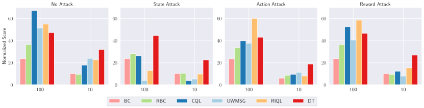
Figure 1: Average normalized scores of offline RL algorithms under random data corruption across three MoJoCo tasks (Halfcheetah, Walker and Hopper) using "medium-replay-v2" datasets. Many offline RL algorithms experience a substantial performance decline when subjected to data corruption. Notably, DT demonstrates superior robustness in the face of state corruption and limited data regimes.

3.1 Motivating Example

As illustrated in Figure 1, we compare DT with various offline RL algorithms under data corruption. We apply random corruption introduced in Section 2.3 on states, actions, and rewards. Specifically, we perturb $30\%$ of the transitions in the dataset and introduce random noise at a scale of 1.0 standard deviation. In addition to the conventional full dataset setting employed in previous studies (Ye et al., 2024b, ; Yang et al., 2024b, ), we also explore a scenario with a reduced dataset, comprising only $10\%$ of the original trajectories. Our results reveal that most offline RL methodologies are susceptible to data corruption, particularly in the limited data setting. In contrast, DT exhibits remarkable robustness to data corruption, particularly in cases of state corruption and all limited dataset settings. This resilience can be attributed to DT’s formulation based on sequence modeling and its supervised training paradigm. We will later discuss more in-depth about the important components impacting the robustness of DT in Section D.1. In the full dataset setting, it is worth noting that DT exhibits slightly lower performance compared to RIQL and UWMSG when subjected to action and reward attacks, indicating room for further improvement.

Overall, the results demonstrate DT can outperform prior imitation-based and temporal-difference based methods without any robustness enhancement. This observation raises an intriguing question:

How can we further unleash the potential of sequential modeling in addressing data corruption with limited dataset in offline RL?

3.2 Robust Decision Transformer

To enhance the robustness of DT against various data corruption, we propose Robust Decision Transformer (RDT) by incorporating three components: embedding dropout (Section 3.2.1), Gaussian weighted learning (Section 3.2.2), and iterative data correction (Section 3.2.3). The overall framework is depicted in Figure 2. Notably, RDT predicts actions and rewards (rather than reward-to-gos) on top of the DT. Given the typically high dimensionality of states, we avoid predicting states to mitigate potential negative impacts. Additionally, rewards provide more direct supervision for the policy compared to reward-to-gos, which are also dependent on future actions.

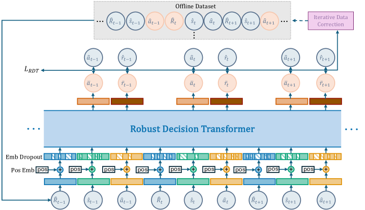
Figure 2: Framework of Robust Decision Transformer (RDT). RDT enhances the robustness of DT against data corruption by incorporating three components on top of DT: embedding dropout, Gaussian weighted learning, and iterative data correction.

3.2.1 Embedding Dropout

In the setting of data corruption, corrupted states, actions, and rewards can supply shifted inputs or erroneous features to the model. This can lead to a performance drop if the model overfits to particular harmful features. Therefore, learning a robust representation is important to enhance the model’s resilience against data corruption scenario. To achieve this, we employ embedding dropout, which encourages the model to learn more robust embedding representations and avoid overfitting (Merity et al.,, 2017).

To clarify, we define three hidden embeddings after the linear projection layer as $h_{R_{t}}$, $h_{s_{t}}$, and $h_{a_{t}}$, represented as:

$$h_{R_{t}}=\phi_{R}(R_{t})+\phi_{t}(t),\quad h_{s_{t}}=\phi_{s}(s_{t})+\phi_{t}(t),\quad h_{a_{t}}=\phi_{a}(a_{t})+\phi_{t}(t).$$

Here, $\phi_{R}$, $\phi_{s}$, and $\phi_{a}$ denote linear projection layers on different elements, while $\phi_{t}(t)$ represents the time-step embedding. Subsequently, we apply randomized dimension dropping on these feature embeddings, resulting in the corresponding masked feature embeddings as follows:

$$\tilde{h}_{R_{t}}=\mathcal{M}(p)\otimes h_{R_{t}},\quad\tilde{h}_{s_{t}}=\mathcal{M}(p)\otimes h_{s_{t}},\quad\tilde{h}_{a_{t}}=\mathcal{M}(p)\otimes h_{a_{t}}.$$ (3)

The function $\mathcal{M}(\cdot)$ takes a probability as input and outputs a binary mask to determine the dimension inclusion. We use the same drop probabilities $p$ for different elements embedding.

3.2.2 Gaussian Weighted Learning

In DT, actions serve as the most crucial supervised information, acting as the labels. Consequently, erroneous actions can directly influence the model through backpropagation. In RDT, we predict both actions and rewards, with rewards helping to reduce overfitting to corrupted action labels. To further mitigate the impact of corrupt data, we aim to reduce the influence of unconfident action and reward labels that could erroneously guide policy learning.

To identify uncertain labels, we adopt a simple but effective method: we use the value of the sample-wise loss to adjust the weight for the DT loss. The underlying insight is that a corrupted label would typically lead to a larger loss. To softly reduce the effect of potentially corrupted labels, we use the Gaussian weight, i.e., a weight that decays exponentially in accordance with the sample’s loss. This is mathematically represented as:

$$w_{a_{t}}^{(i)}=e^{-\beta_{a}\cdot\delta_{a_{t}}^{2}}, w_{r_{t}}^{(i)}=e^{-\beta_{r}\cdot\delta_{r_{t}}^{2}},\text{ where }\delta_{a_{t}}=\text{no\_grad}(\|\pi_{\theta}(\hat{\tau}_{t-K+1:t-1}^{(i)},\hat{R}_{t}^{(i)},\hat{s}_{t}^{(i)})-\hat{a}_{t}^{(i)}\|_{2}),$$ (4)

$$\delta_{r_{t}}=\text{no\_grad}(\|\pi_{\theta}(\hat{\tau}_{t-K+1:t-1}^{(i)},\hat{R}_{t}^{(i)},\hat{s}_{t}^{(i)},\hat{a}_{t}^{(i)})-\hat{r}_{t}^{(i)}\|_{2}),$$

In this equation, $\delta_{a_{t}}$ and $\delta_{r_{t}}$ represent the detached prediction errors at step $t$. The variables $\beta_{a}\geq 0,\beta_{r}\geq 0$ act as the temperature coefficients, providing flexibility to control the "blurring" effect of the Gaussian weights. With a larger value, more samples would be down-weighted. The loss function of RDT is expressed as follows:

$$\mathcal{L}_{RDT}(\theta)=\mathbb{E}_{\hat{\tau}^{(i)}\sim\mathcal{D}} \Bigg{[}\frac{1}{K}\sum_{t=0}^{K-1}\Big{[}w_{a_{t}}^{(i)}\|\pi_{\theta}(\hat{\tau}_{t-K+1:t-1}^{(i)},\hat{R}_{t}^{(i)},\hat{s}_{t}^{(i)})-\hat{a}_{t}^{(i)}\|_{2}^{2}$$ (5)

$$+w_{r_{t}}^{(i)}\|\pi_{\theta}(\hat{\tau}_{t-K+1:t-1}^{(i)},\hat{R}_{t}^{(i)},\hat{s}_{t}^{(i)},\hat{a}_{t}^{(i)})-\hat{r}_{t}^{(i)}\|_{2}^{2}\Big{]}\Bigg{]}$$

Gaussian weighted learning enables us to mitigate the detrimental effects of corrupted labels, thereby enhancing the algorithm’s robustness.

3.2.3 Iterative Data Correction

While Gaussian weighted learning has significantly reduced the impact of corrupted labels, these erroneous data can still influence the policy as they still serve as inputs for policy learning. We propose iteratively correcting corrupted data in the dataset using the model’s predictions to bring the data closer to their true values in the next iteration. This method can further minimize the detrimental effects of corruption and can be implemented to correct reward-to-gos, states, and actions in the sequence modeling framework. In RDT, it is straightforward to correct the actions and rewards in the dataset, and recalculate the reward-to-gos using corrected rewards. Therefore, our implementation focuses on correcting states and reward-to-gos in the datasets, leaving better data correction methods for states for future work.

Initially, we store the distribution information of prediction error $\delta$ in Eq.4 throughout the learning phase to preserve the mean $\mu_{\delta}$ and variance $\sigma^{2}_{\delta}$ of actions and rewards, updating them with every batch of samples. Our hypothesis is that the prediction error $\delta$ between predicted and clean label actions should exhibit consistency after sufficient training. Therefore, if erroneous label actions are encountered, $\delta$ will deviate from the mean $\mu_{\delta}$, behaving like outliers. This deviation essentially enables us to detect and correct the corrupted action using the distributional information of $\delta$.

Taking actions as an example, to detect corrupted actions, we calculate the $z$-score, denoted by $z^{(i)}=\frac{\delta^{(i)}-\mu_{\delta}}{\sigma_{\delta}}$, for each sampled action $\hat{a}^{(i)}$ and the current policy. If the condition $z^{(i)}>\zeta\cdot\sigma_{\delta}$ is met for any given action $\hat{a}^{(i)}$, we infer that the action $\hat{a}^{(i)}$ has been corrupted. We then permanently replace $\hat{a}^{(i)}$ in the dataset with the predicted action. Correcting rewards follows a similar process, with the additional step of recalculating the reward-to-gos. The hyperparameter $\zeta$ determines the detection thresholds: a smaller $\zeta$ will classify more samples as corrupted data, while a larger $\zeta$ results in fewer modifications to the dataset.

4 Experiments

In this section, we conduct a comprehensive empirical assessment of RDT to address the following questions: 1) How does RDT perform under several data corruption scenarios during the training phase? 2) Is RDT robust to different data corruption rates and scales? 3) What is the impact of each component of RDT on its overall performance? 4) How does RDT perform when faced with observation perturbations during the testing phase?

4.1 Experimental Setups

We evaluate RDT across a variety of tasks, such as MoJoCo ("medium-replay-v2" datasets), KitChen, and Adroit (Fu et al.,, 2020). Two types of data corruption during the training phase are simulated: random corruption and adversarial corruption, attacking states, actions, and rewards, respectively. The corruption rate is set to $0.3$ and the corruption scale is $\epsilon=1.0$ for the main results. Data corruption is introduced in Section 2.3 and more details can be found in Section C.1. Additionally, we find that the data corruption problem can exacerbate when the data is limited. To simulate this scenario, we down-sample on both MuJoCo and Adroit tasks, referred to as MuJoCo (10%) and Adroit (1%), Specifically, we randomly select 10% (and 1%) of the trajectories from MuJoCo (and Adroit) tasks and conduct data corruption on the sampled data. We do not down-sample the Kitchen dataset because it already has a limited dataset size. All considered tasks have a similar dataset size of about 20,000 transitions, except for the original MuJoCo task, which includes a larger dataset.

We compare RDT with several SOTA offline RL algorithms and robust methods, namely BC, RBC (Sasaki and Yamashina,, 2020), DeFog (Hu et al.,, 2023), CQL (Kumar et al.,, 2020), UWMSG (Ye et al., 2024b, ), RIQL (Yang et al., 2024b, ), and DT (Chen et al.,, 2021). BC and RBC employ behavior cloning loss within an MLP-based model for policy learning, while DeFog and DT utilize a Transformer architecture. We implement RBC with our Gaussian-weighted learning as an instance of  (Sasaki and Yamashina,, 2020). In Appendix D.1, we investigate the robustness of DT across various critical parameters. Drawing from these findings on DT’s robustness, we establish a default implementation of DT, DeFog, RDT with a sequence length of 20 and a block number of 3. To ensure the validity of the findings, each experiment is repeated using 4 different random seeds.

Table 1: Average normalized performance under random data corruption.

Task Attack Element BC RBC DeFog CQL UWMSG RIQL DT RDT (ours) MuJoCo state 24.1 31.5 19.5 22.0 5.7 22.7 45.5 49.1 action 26.9 29.6 49.7 56.9 52.3 57.8 52.4 54.1 reward 28.1 29.1 42.9 58.6 51.3 60.4 52.7 54.8 MuJoCo (10%) state 9.5 8.0 16.2 4.5 6.8 9.7 21.4 23.1 action 9.0 7.4 15.4 10.3 19.3 12.8 19.4 25.9 reward 10.0 11.0 16.2 12.7 9.4 18.7 27.5 31.6 KitChen state 39.9 29.8 20.8 5.1 0.1 22.5 31.2 43.1 action 37.9 37.3 13.7 3.6 0.0 30.6 28.8 40.4 reward 45.3 50.3 19.7 0.1 0.0 43.0 49.2 52.6 Adroit (1%) state 54.5 74.2 72.9 -0.1 -0.1 23.1 86.9 96.4 action 35.9 71.8 83.9 -0.1 -0.1 12.6 76.8 99.1 reward 34.7 88.6 88.8 -0.1 -0.1 22.7 84.7 100.9 Average 29.6 39.0 38.3 14.5 12.1 28.1 48.0 55.9

4.2 Evaluation under Various Data Corruption

Random Data Corruption.

To address the first question, we evaluate the RDT and baselines on random data corruption across a diverse set of task groups. Each group consists of three datasets, and the mean normalized score was calculated to represent the final outcomes. As shown in Table 1, RDT demonstrates superior performance in handling data corruption, achieving the highest score in 10 out of 12 settings, particularly in the challenging Kitchen and Adroit tasks. Notably, across all task groups, RDT outperforms DT, underscoring its effectiveness in reducing DT’s sensitivity to data corruption across all elements. Moreover, RBC significantly outperforms BC, further highlighting the effectiveness of Gaussian weighted learning. However, prior offline RL methods, such as RIQL and UWMSG, fail to yield satisfactory results and even underperform BC overall, despite showing enhanced performance on the full MuJoCo dataset. This indicates that temporal difference methods are dependent on large-scale datasets.

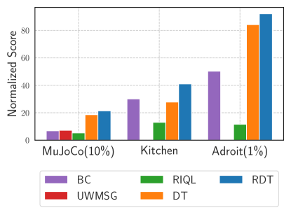
Figure 3: Results under mixed random data corruption.

Mixed Random Data Corruption.

To present a more challenging setting for the robustness of RDT, we conduct an experiment under the mixed random data corruption setting. In this setting, all three elements - states, actions, and rewards - are corrupted at a rate of $0.3$ and a scale of $\epsilon=1.0$. The experimental results are shown in Figure 3. Remarkably, RDT consistently outperforms other baseline models across all tasks, thereby highlighting its superior stability even when faced with simultaneous and diverse random data corruption. Especially on the challenging Kitchen task, RDT outperforms DT by an impressive margin of approximately 40$\%$.

Adversarial Data Corruption.

We further extend the analysis to examine the robustness of the RDT under adversarial data corruption. We employ the same hyperparameters for RDT as those utilized in the random data corruption scenarios, demonstrating RDT’s advantage of not requiring meticulous hyperparameter tuning. As evidenced in Table 2, RDT consistently showcases a robust performance by attaining the highest scores in 8 out of 9 settings and sustaining the top average performance. Notably, RDT stands out for enhancing the average score by $28.9\%$ compared to DT in the adversarial action corruption scenario. Intriguingly, temporal-difference methods like CQL, UWMSG, and RIQL perform notably worse than BC and sequence modeling methods such as DT and DeFog, highlighting the promise of sequence modeling approaches. We provide detailed results for each task in Appendix D for comprehensive analysis.

Table 2: Average normalized performance under adversarial data corruption.

Task Attack Element BC RBC DeFog CQL UWMSG RIQL DT RDT (ours) MuJoCo (10%) state 10.8 10.9 8.7 4.5 13.4 11.0 22.8 22.6 action 5.6 6.4 10.4 11.4 18.1 7.1 12.9 17.5 reward 10.0 10.8 13.8 11.7 7.8 18.3 27.7 29.1 KitChen state 33.5 37.2 20.8 1.8 0.0 28.5 36.4 42.3 action 5.0 7.8 13.7 0.7 5.1 4.4 8.1 33.7 reward 45.3 43.4 19.7 0.0 0.0 38.8 49.8 54.0 Adroit (1%) state 66.6 70.5 80.5 -0.1 -0.1 37.0 90.4 96.8 action 19.3 24.3 54.2 -0.1 -0.1 4.4 35.2 90.2 reward 34.7 84.0 82.9 -0.1 -0.1 26.4 87.9 91.4 Average 25.6 32.8 33.9 3.3 4.9 19.5 41.2 53.1

4.3 Varying Corruption Rates and Scales

In the above experiments, we evaluate the effectiveness of RDT under a data corruption rate of $0.3$ and a scale of $1.0$. We further examine the robustness of RDT under different corruption rates from $\{0.0,0.1,0.3,0.5\}$ and scales from $\{0.0,1.0,2.0\}$. As illustrated in Figure 4, RDT consistently delivers superior performance compared to other baselines across different corruption rates and scales. However, we did observe a decline in RDT’s performance when it encountered state corruption with high rates. This decline can be attributed to the distortion of the state’s distribution caused by the high corruption rates, resulting in a significant deviation from the clean test environment to the corrupted datasets. Enhancing the robustness of RDT against state corruption, especially under high corruption rates and scales, holds potential for future advancements.

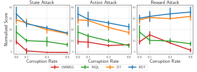
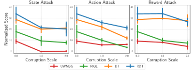
Figure 4: Results under various data corruption rates (a) and scales (b) on "walker2d-medium-replay".

4.4 Ablation Study

We conduct comprehensive ablation studies to analyze the impact of each component on RDT’s robustness. For evaluation, we use the "walker2d-medium-replay", "kitchen-compete", and "relocate-exper"’ datasets. Specifically, we compare several variants of RDT: (1) DT(RP), which incorporates reward prediction in addition to the original DT; (2) DT(RP) w. ED, which adds embedding dropout to DT(RP); (3) DT(RP) w. GWL, which applies Gaussian weighted learning on top of DT(RP); and (4) DT(RP) w. IDC, which integrates only the iterative data correction method.

We evaluate the performance of these variants under different data corruption scenarios, as depicted in Figure 5. In summary, all variants demonstrate improvements over DT(RP), proving the effectiveness of the individual components. Notably, Gaussian weighted learning appears to provide the most significant contribution, particularly under reward attack. However, it is important to note that none of these tailored models outperform RDT, indicating that the integration of all proposed techniques is crucial for achieving optimal robustness. Additionally, we provide ablation results on reward prediction in Section D.2, which demonstrate that reward prediction also brings improvements under state and action corruption compared to DT.

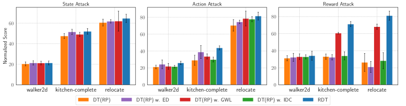
Figure 5: Ablation study on the impact of different proposed components.

4.5 Evaluation under Observation Perturbation during the Testing Phase

In this section, we further investigate the robustness of RDT when deployed in perturbed environments after being trained on corrupted data, a challenging setting that includes both training-time and testing-time attacks. To address this, we evaluate RDT under two types of observation perturbations during the testing phase: random and action diff, following prior works (Yang et al., 2022a, ; Zhang et al.,, 2020). The perturbation scale is used to control the extent of influence on the observation. Detailed implementation of observation perturbations during the testing phase is provided in Section C.2.

The comparison results are presented in Figure 6, where all algorithms are trained on the offline dataset with action corruption and evaluated under observation perturbation. These results demonstrate the superior robustness of RDT under the two types of observation perturbations, maintaining stability even at a high perturbation scale of 0.5. Notably, RORL (Yang et al., 2022a, ), a SOTA offline RL method designed to tackle testing-time observation perturbation, fails to perform effectively on these tasks. Additionally, DT and RIQL experience significant performance drops as the perturbation scale increases. Further results comparing different algorithms trained on offline datasets with state or reward corruption can be found in Section D.4.

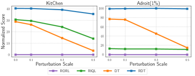
(a) Random observation perturbation.

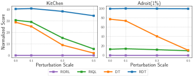
(b) "Action diff" observation perturbation.

Figure 6: Performance under various observation perturbation scales during the testing phase. All the algorithms are trained under random action corruption during the training phase.

5 Related Work

Robust Offline RL.

In offline RL, several works have focused on testing-time robustness against environment shifts (Shi and Chi,, 2022; Yang et al., 2022a, ; Panaganti et al.,, 2022; Zhihe and Xu,, 2023). Regarding training-time robustness, Li et al., (2023) explore various types of reward attacks in offline RL and find that certain biases can inadvertently enhance the robustness of offline RL methods to reward corruption. From a theoretical perspective, Zhang et al., (2022) propose a robust offline RL algorithm utilizing robust supervised learning oracles. Additionally, Ye et al., 2024b employ uncertainty weighting to address reward and dynamics corruption, providing theoretical guarantees. The most relevant research by Yang et al., 2024b employs the Huber loss to handle heavy-tailedness and utilizes quantile estimators to balance penalization for corrupted data. Furthermore, Mandal et al., (2024); Liang et al., (2024) enhance the resilience of offline algorithms within the RLHF framework. It is important to note that these studies primarily focus on enhancing temporal difference methods, with no emphasis on leveraging sequence modeling techniques to tackle data corruption.

Transformers for RL.

Recent research has redefined offline RL decision-making as a sequence modeling problem using Transformer architectures (Chen et al.,, 2021; Janner et al.,, 2021). Unlike traditional RL methods, these studies treat RL as a supervised learning task at a trajectory level. A seminal work, Decision Transformer (DT) (Chen et al.,, 2021), uses trajectory sequences to predict subsequent actions. Trajectory Transformer (Janner et al.,, 2021) discretizes input sequences into tokens and employs beam search to predict the next action. These efforts have led to subsequent advancements. For instance, Prompt DT (Xu et al.,, 2022) integrates demonstrations for better generalization, while Xie et al., (2023) introduce pre-training with future trajectory information. Q-learning DT (Yamagata et al.,, 2023) refines return-to-go using Q-values, and Agentic Transformer (Liu and Abbeel,, 2023) uses hindsight to relabel target returns. LaMo (Shi et al.,, 2023) leverages pre-trained language models for offline RL, and DeFog (Hu et al.,, 2022) addresses robustness in specific frame-dropping scenarios. Our work deviates from these approaches by focusing on improving robustness against data corruption in offline RL.

6 Conclusion

In this study, we investigate the robustness of offline RL algorithms under various data corruptions, with a specific focus on sequence modeling methods. Our empirical evidence suggests that current offline RL algorithms based on temporal difference learning exhibit significant susceptibility to data corruption, particularly in scenarios with limited data. To address this issue, we introduce the Robust Decision Transformer (RDT), a novel robust offline RL algorithm developed from the perspective of sequence modeling. Our comprehensive experiments highlight RDT’s exceptional robustness against both random and adversarial data corruption, across different corruption ratios and scales. Furthermore, we demonstrate RDT’s superiority in handling both training-time and testing-time attacks. We hope that our findings will inspire further research into the exploration of using sequence modeling methods to address data corruption challenges in increasingly complex and realistic scenarios.

Appendix A Algorithm Pseudocode

To provide an overview and better understanding, we detail the implementation of Robust Decision Transformer (RDT) in  Algorithm 1.

Algorithm 1 Robust Decision Transformer (RDT)

1:Offline dataset $\mathcal{D}$, sequence model $\pi_{\theta}$, initialed mean $\mu_{\delta}$ and variance $\sigma^{2}_{\delta}$.

2:for training step$=1,2,\ldots,T$ do

3:     Extract batch $\tau_{t:t+K-1}$ from the offline dataset $\mathcal{D}$.

4:     Update sequence model $\pi_{\theta}$ based on Eq. 5.

5:     Compute prediction errors $\delta_{a_{t}}$ and $\delta_{r_{t}}$ in batch data.

6:     Update corresponding mean $\mu_{\delta}$ and variance $\sigma^{2}_{\delta}$

7:end for

8:if correction phase begins then

9:     Evaluate the $z$-score to identify the corrupted action $\hat{a}^{(i)}_{t}$ and reward $\hat{r}^{(i)}_{t}$.

10:     Substitute corrupted actions and rewards with the predicted actions and rewards in dataset $\mathcal{D}$.

11:end if

Appendix B Additional Related Works

Offline RL. Maintaining proximity between the policy and data distribution is essential in offline RL, as distributional shifts can lead to erroneous estimations (Levine et al.,, 2020). To counter this, offline RL algorithms are primarily divided into two categories. The first category focuses on policy constraints on the learned policy (Wang et al.,, 2018; Fujimoto et al.,, 2019; Li et al.,, 2020; Fujimoto and Gu,, 2021; Kostrikov et al.,, 2021; Emmons et al.,, 2021; Yang et al., 2022b, ; Sun et al.,, 2024; Xu et al.,, 2023; Park et al.,, 2024). The other category learns pessimistic value functions to penalize OOD actions (Kumar et al.,, 2020; Yu et al.,, 2020; An et al.,, 2021; Bai et al.,, 2022; Yang et al., 2022a, ; Ghasemipour et al.,, 2022; Sun et al.,, 2022; Nikulin et al.,, 2023; Huang et al.,, 2024). To enhance the potential of offline RL in handling more complex tasks, recent research has integrated advanced techniques like GAN (Vuong et al.,, 2022; Wang et al.,, 2023), transformers (Chen et al.,, 2021; Chebotar et al.,, 2023; Yamagata et al.,, 2023) and diffusion models (Janner et al.,, 2022; Hansen-Estruch et al.,, 2023; Wang et al.,, 2022).

Appendix C Implementation Details

C.1 Data Corruption Details during Training Phase

Our study utilizes both random and adversarial corruption across three elements: states, actions, and rewards. We consider a range of tasks including MuJoCo, Kitchen, and Adroit. Particularly, we utilize the “medium-replay-v2” datasets in the MuJoCo tasks with sampling ratios of 100% and 10%, the “expert-v0” datasets in the Adroit tasks with a sampling ratio of 1%, and we employ full datasets for the tasks in the Kitchen due to their already limited data size. These datasets (Fu et al.,, 2020) are collected either during the training process of an SAC agent or from expert demonstrations, thereby providing highly diverse and representative tasks of the real world. To control the overall level of corruption within the datasets, we introduce two parameters $c$ and $\epsilon$ following previous work (Yang et al., 2024b, ). The parameter $c$ signifies the rate of corrupted data within a dataset, whilst $\epsilon$ represents the scale of corruption observed across each dimension. We outline three types of random data corruption and present a comprehensive overview of a mixed corruption approach as follows. Note that in our setting, only three independent elements (i.e., states, actions, and rewards) are considered under the trajectory-based storage approach.

• Random state attack: We randomly sample $c\cdot N\cdot T$ states from all trajectories, where $N$ refer to the number of trajectories and $T$ represents the number of steps in a trajectory. We then modify the selected state to $\hat{s}=s+\lambda\cdot\text{std}(s),\lambda\sim\text{Uniform}[-\epsilon,\epsilon]^{d_{s}}$. Here, $d_{s}$ represents the dimension of states, and “$\text{std}(s)$” is the $d_{s}$-dimensional standard deviation of all states in the offline dataset. The noise is scaled according to the standard deviation of each dimension and is independently added to each respective dimension.

• Random action attack: We randomly select $c\cdot N\cdot T$ actions from all given trajectories, and modify the action to $\hat{a}=a+\lambda\cdot\text{std}(a),\lambda\sim\text{Uniform}[-\epsilon,\epsilon]^{d_{a}}$, where $d_{a}$ represents the dimension of actions and “$\text{std}(a)$” is the $d_{a}$-dimensional standard deviation of all actions in the offline dataset.

• Random reward attack: We randomly sample $c\cdot N\cdot T$ rewards from all given trajectories, and modify the reward to $\hat{r}\sim\text{Uniform}[-30\cdot\epsilon,30\cdot\epsilon]$. We multiply by 30 because we have noticed that offline RL algorithms tend to be resilient to small-scale random reward corruption (also observed in (Li et al.,, 2023)), but would fail when faced with large-scale random reward corruption.

In addition, three types of adversarial data corruption are detailed as follows:

• Adversarial state attack: We first pretrain IQL agents with a Q function $Q_{p}$ and policy function $\pi_{p}$ on clean datasets. Then, we randomly sample $c\cdot N\cdot T$ states, and modify them to $\hat{s}=\min_{\hat{s}\in\mathbb{B}_{d}(s,\epsilon)}Q_{p}(\hat{s},a)$. Here, $\mathbb{B}_{d}(s,\epsilon)=\{\hat{s}||\hat{s}-s|\leq\epsilon\cdot\text{std}(s)\}$ regularizes the maximum difference for each state dimension. The optimization is implemented through Projected Gradient Descent similar to prior works (Madry et al.,, 2017; Zhang et al.,, 2020; Yang et al., 2024b, ). Specifically, We first initialize a learnable vector $z\in[-\epsilon,\epsilon]^{d_{s}}$, and then conduct a 100-step gradient descent with a step size of 0.01 for $\hat{s}=s+z\cdot\text{std}(s)$, and clip each dimension of $z$ within the range $[-\epsilon,\epsilon]$ after each update.

• Adversarial action attack: We use the pretrained IQL agent with a Q function $Q_{p}$ and a policy function $\pi_{p}$. Then, we randomly sample $c\cdot N\cdot T$ actions, and modify them to $\hat{a}=\min_{\hat{a}\in\mathbb{B}_{d}(a,\epsilon)}Q_{p}(s,\hat{a})$. Here, $\mathbb{B}_{d}(a,\epsilon)=\{\hat{a}||\hat{a}-a|\leq\epsilon\cdot\text{std}(a)\}$ regularizes the maximum difference for each action dimension. The optimization is implemented through Projected Gradient Descent, as discussed above.

• Adversarial reward attack: We randomly sample $c\cdot N\cdot T$ rewards, and directly modify them to: $\hat{r}=-\epsilon\times r$.

C.2 Observation Perturbation Details during the Testing Phase

We evaluate the Robust Decision Transformer (RDT) under two types of perturbations during the testing phase: random and action diff perturbations, as described in prior works (Yang et al., 2022a, ; Zhang et al.,, 2020). Both perturbation types target the observations during the testing phase. The detailed implementations are as follows:

• Random: We sample perturbed states within an $l_{\infty}$ ball of norm $\epsilon$. Specifically, we create the perturbation set $\mathbb{B}_{d}(s,\epsilon)=\{\hat{s}:d(s,\hat{s})\leq\epsilon\}$ for state $s$, where $d(\cdot)$ is the $l_{\infty}$ norm, and sample one perturbed state to return to the agent.

• Action Diff: This is an adversarial attack based on the pretrained IQL deterministic policy $\mu(s)$. We first sample 50 perturbed states within an $l_{\infty}$ ball of norm $\epsilon$ and then find the one that maximizes the difference in actions: $\max_{\hat{s}\in\mathbb{B}_{d}(s,\epsilon)}||\mu(s)-\mu(\hat{s})||^{2}$.

The parameter $\epsilon$ controls the extent of the observation perturbation. In this experiment, we first train RDT under different data corruption scenarios and then evaluate its performance in environments subjected to observation perturbation.

C.3 Implementation Details of RDT

We implement the DT and RDT algorithms using the existing code base. Specifically. we build the network with 3 Transformer blocks, incorporating one MLP embedding layer for each key element: state, action, and return-to-go. We update the neural network using the AdamW optimizer, with a learning rate set at $1\times 10^{-4}$ and a weight decay of $1\times 10^{-4}$. The batch size is set to 64, with a sequence length of 20, to ensure effective and efficient training. To maintain stability during training, we adopt the state normalization as in (Yang et al., 2024b, ). During the training phase, we train DeFog, DT and RDT for 100 epochs and other baselines with 1000 epochs. Each epoch is characterized by 1000 gradient steps. For evaluative purposes, we rollout each agent in the clean environment across 10 trajectories, each with a maximum length of 1000, and we average the returns from these rollouts for comparison. We ensure the consistency and reliability of our reported results by averaging them over 4 unique random seeds. All experiments are conducted on 8 P40 GPUs.

As for the hyperparameters of RDT, we configure the values for the embedding dropout probability as $p$, Gaussian Weighted coefficient $\beta_{a}$ and $\beta_{r}$, and iterative data correction threshold $\zeta$ through the sweeping mechanism. We start the iterative data correction at the 50th epoch for all tasks. We use iterative action correction exclusively for action corruption and iterative reward correction exclusively for reward corruption; therefore, only a single $\zeta$ value is shown in Table 3. It’s noteworthy that we do not conduct a hyperparameter search for individual datasets; instead, we select hyperparameters that apply to the entire task group. As such, RDT doesn’t require extensive hyperparameter tuning as previous methods. The exact hyperparameters used for the random corruption experiment are detailed in Table 3. We employ the same hyperparameters for the adversarial corruption experiment, further attesting to the robustness and stability of RDT.

Table 3: Hyperparameters used for RDT under the random corruption benchmark.

Tasks	Attack Element	$p$	($\beta_{a}$, $\beta_{r}$)	$\zeta$
MuJoCo	state	0.0	(1.0, 10.0)	$-$
	action	0.0	(0.1, 0.0)	3.0
	reward	0.0	(0.1, 0.1)	6.0
MuJoCo (10%)	state	0.1	(0.1, 0.1)	$-$
	action	0.1	(0.1, 0.1)	5.0
	reward	0.2	(0.1, 0.1)	6.0
Kitchen	state	0.1	(10.0, 10.0)	$-$
	action	0.1	(10.0, 10.0)	1.5
	reward	0.0	(10.0, 10.0)	3.0
Adroit (1%)	state	0.1	(0.1, 0.0)	$-$
	action	0.1	(10.0, 0.0)	6.0
	reward	0.1	(0.1, 0.1)	6.0

Appendix D Additional Experiments

D.1 Impact of Decision Transformer’s Hyperparameters

We aim to understand the robustness characteristic of sequence modeling. The key feature of the DT is its utilization of sequence modeling, with the incorporation of the transformer model. Consequently, we identify two crucial factors that may influence the performance of DT in the context of sequence modeling: the model structure and the input data.

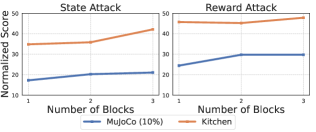
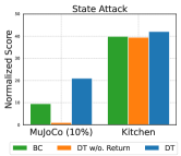
Figure 7: Ablation study on the robustness of DT. (a) Analyzing the influence of block number of DT while keeping sequence length with 20. (b) The effect of sequence length while maintaining 3 transformer blocks. (c) Investigation on how the return-to-go impacts DT. We create the variant DT w/o. Return which excludes the use of return-to-go as inputs.

We explore the influence of the model’s structure by modifying the number of Transformer blocks in DT. As depicted in Figure 7(a), the performance on both MuJoCo and Kitchen tasks consistently improves with an increase in the number of blocks. Therefore, the enhancement can be partially attributed to the increased capabilities of the larger model.

We also examine the impact of the inputs for the sequence model. There are two primary differences between the input of DT and that of conventional BC. DT predicts actions based on historical data and return-to-go elements, whereas BC relies solely on the current states. To assess the influence of these factors, we independently evaluate the impact of the length of history and return-to-go elements. The results in Figure 7(b) and (c) reflect that Kitchen tasks favor longer historical input and are less reliant on return-to-go elements. Conversely, MuJoCo tasks demonstrated a different trend. This discrepancy could be due to the sparse reward structure of Kitchen tasks, where return-to-go elements do not provide sufficient information, leading the agent to rely more heavily on historical data for policy learning. In contrast, MuJoCo tasks, with their denser reward structures, rely more on return-to-go elements for optimal policy learning.

In summary, the robustness of DT can be attributed to the model capacity, history length, and the return-to-go conditioning. Based on this findings on the robustness of DT, we adopt a sequence length of 20 and a block number of 3 as the default implementation for all sequence modeling methods, including DT, DeFog, and RDT.

D.2 Ablation Study on Reward Prediction

The nature of the sequential model allows us to predict not only actions but also other elements such as state and return-to-go. Previous studies have shown that predicting these additional elements does not significantly enhance performance Chen et al., (2021). However, we find that predicting rewards can provide advantages in the context of data corruption. We introduce DT(RP), a variant of the original Decision Transformer (DT), which predicts rewards in addition to actions. As illustrated in Figure 8, predicting rewards indeed improves performance under state and action corruption conditions. However, DT(RP) performs poorly under reward corruption due to the degraded quality of reward labels. This issue can be mitigated via embedding dropout, Gaussian weighted learning, and iterative data correction in RDT.

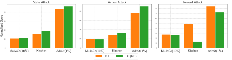
Figure 8: Ablation study on the impact of reward prediction.

D.3 Ablation Study on Hyperparameters

We conducted experiments to investigate the impact of hyperparameters of the Robust Decision Transformer (RDT) under scenarios of action corruption.

In our study of the embedding dropout technique, depicted in Figure 9(a), we discovered that applying a moderate dropout probability (e.g., 0.1) to embeddings enhances resilience against data corruption. However, a larger dropout rate ($\geq$ 0.5) can lead to performance degradation.

As shown in Figure 9(b), regarding the Gaussian weighted coefficient $\beta_{a}$, the walker2d task favors lower values of $\beta_{a}$ such as 0.1, while the kitchen and relocate tasks favor larger $\beta_{a}$ values, suggesting that these tasks are more impacted by Gaussian weight learning.

In terms of the iterative data correction threshold $\zeta$, the results are highlighted in Figure 9(c). The walker2d and kitchen tasks favor lower values of $\zeta$, whereas the relocate task exhibits the opposite preference. Notably, in the relocate task, RDT shows markedly enhanced performance after correcting outliers (with $\zeta\geq 5$) in the dataset.

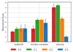
(a) Embedding drop $p$

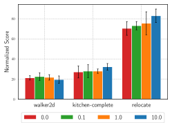
(b) Gaussian weight coefficient $\beta_{a}$

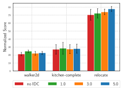
(c) Iterative correction threshold $\zeta$

Figure 9: Ablation study on the impact of hyperparameters under action corruption scenario.

D.4 Additional Results under Observation Perturbation during the Testing Phase

To further demonstrate the robustness of RDT, we conducted additional evaluations under observation perturbation during the testing phase. Specifically, we compared different algorithms trained with offline datasets under conditions of state or reward corruption in perturbed environments. As shown in Figures 10 and 11, RDT consistently maintained superior performance and robustness across observation perturbations in both the Kitchen and Adroit tasks.

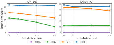
(a) "Random" observation perturbation.

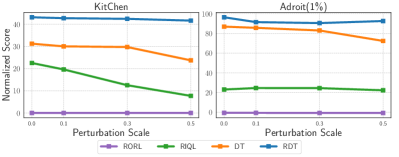
(b) "Action diff” observation perturbation.

Figure 10: Performance under varying observation perturbation scales during the testing phase. All the algorithms are trained under random state corruption during the training phase.

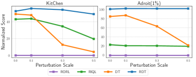
(a) "Random" observation perturbation.

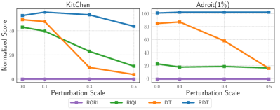
(b) "Action diff" observation perturbation.

Figure 11: Performance under varying observation perturbation scales during the testing phase. All the algorithms are trained under random reward corruption during the training phase.

D.5 Training Time

We trained all algorithms on the same P40 GPU, and the training times are presented in Table 4. As expected, BC has the shortest epoch time due to its simplicity. Notably, RDT requires only slightly more time per epoch than DT because it incorporates three robust techniques. Although RIQL requires less time per epoch than RDT, it necessitates 10 times more epochs to converge and still does not achieve satisfactory performance in the limited data regime. In conclusion, RDT achieves superior performance and robustness without imposing significant computational costs in terms of total training time.

Table 4: Training time on the "walker2d-medium-replay" dataset.

Method	BC	CQL	UWMSG	RIQL	DT	RDT (ours)
Epoch Num	1000	1000	1000	1000	100	100
Epoch Time (s)	3.7	33.8	22.2	14.9	44.0	46.1
Total Time (h)	1.03	9.39	6.17	4.14	1.22	1.28

D.6 Detailed Results for the Main Experiments

The detailed outcomes of each task, under both random and adversarial data corruption, can be found in Table 5 and Table 6 respectively. For HalfCheetah, Hopper, and Walker2D tasks, we have utilized the "medium-replay-v2" datasets, while the "expert-v0" datasets have been used for Door, Hammer, and Relocate tasks. Notably, RDT consistently outperforms baselines in the majority of tasks, achieving the best average performance and demonstrating its robustness and superiority, particularly under the adversarial data corruption.

Table 5: Detailed performance under random data corruption.

Environment Attack Element BC RBC DeFog CQL UWMSG RIQL DT RDT (ours) halfcheetah state 33.7$\pm$0.6 33.0$\pm$2.7 15.8$\pm$3.8 16.7$\pm$1.2 1.1$\pm$0.8 19.9$\pm$2.1 29.7$\pm$2.2 28.1$\pm$0.8 action 34.9$\pm$2.9 35.6$\pm$0.5 34.2$\pm$2.4 44.5$\pm$0.3 49.9$\pm$0.7 41.3$\pm$1.4 36.6$\pm$0.9 35.7$\pm$1.0 reward 36.0$\pm$1.2 34.8$\pm$2.5 33.5$\pm$3.7 44.1$\pm$0.3 37.2$\pm$5.8 42.7$\pm$0.9 38.9$\pm$0.6 37.7$\pm$1.1 hopper state 25.4$\pm$16.0 33.1$\pm$8.7 24.0$\pm$9.0 21.8$\pm$5.9 16.4$\pm$5.0 34.0$\pm$13. 53.7$\pm$11.6 64.6$\pm$6.4 action 25.3$\pm$11.8 33.5$\pm$12.2 52.9$\pm$17.8 55.4$\pm$7.9 49.8$\pm$12.2 59.6$\pm$12.7 59.4$\pm$1.7 66.0$\pm$5.6 reward 28.2$\pm$5.6 33.9$\pm$13.2 45.1$\pm$13.1 57.2$\pm$14.4 65.4$\pm$26.0 59.6$\pm$4.8 57.7$\pm$11.6 63.8$\pm$11.3 walker2d state 13.1$\pm$8.0 28.5$\pm$7.6 18.5$\pm$3.5 27.6$\pm$10.2 -0.5$\pm$0.3 14.2$\pm$1.2 53.2$\pm$10.2 54.5$\pm$2.3 action 19.6$\pm$9.2 19.6$\pm$9.2 61.9$\pm$2.8 70.8$\pm$5.3 57.1$\pm$10.4 72.6$\pm$17.3 61.2$\pm$6.7 60.6$\pm$2.9 reward 20.1$\pm$4.8 18.6$\pm$4.7 50.2$\pm$14.8 74.6$\pm$3.0 51.3$\pm$10.6 79.0$\pm$5.8 61.4$\pm$6.5 62.9$\pm$5.6 halfcheetah (10%) state 5.2$\pm$1.6 1.5$\pm$0.2 3.9$\pm$1.0 11.3$\pm$3.4 5.4$\pm$1.2 4.4$\pm$0.9 7.0$\pm$0.5 8.0$\pm$0.5 action 1.8$\pm$0.2 0.6$\pm$0.1 8.7$\pm$1.6 28.4$\pm$3.2 11.7$\pm$3.4 2.3$\pm$0.6 4.3$\pm$0.3 13.8$\pm$2.3 reward 4.4$\pm$0.8 1.9$\pm$0.2 12.4$\pm$1.7 34.2$\pm$1.0 2.2$\pm$0.7 6.1$\pm$1.2 12.7$\pm$1.0 16.3$\pm$2.4 hopper (10%) state 15.0$\pm$0.6 14.4$\pm$2.0 15.6$\pm$6.5 2.0$\pm$0.4 15.6$\pm$8.0 15.5$\pm$5.4 37.3$\pm$1.1 40.0$\pm$3.2 action 19.2$\pm$3.6 17.7$\pm$1.2 23.7$\pm$4.8 1.8$\pm$0.0 40.7$\pm$5.9 26.3$\pm$2.8 32.1$\pm$1.9 37.9$\pm$7.9 reward 15.1$\pm$0.7 21.1$\pm$0.7 19.2$\pm$10.2 2.6$\pm$0.9 18.2$\pm$2.8 40.2$\pm$2.6 39.9$\pm$2.8 44.3$\pm$4.7 walker2d (10%) state 8.2$\pm$1.8 8.1$\pm$0.9 10.6$\pm$2.2 0.3$\pm$0.7 -0.5$\pm$0.4 9.2$\pm$4.4 19.9$\pm$3.4 21.3$\pm$1.9 action 6.1$\pm$1.0 4.0$\pm$1.6 13.7$\pm$4.7 0.7$\pm$0.9 5.6$\pm$1.2 9.8$\pm$1.9 21.9$\pm$2.7 25.9$\pm$2.0 reward 10.4$\pm$1.6 9.9$\pm$1.5 17.0$\pm$2.5 1.2$\pm$1.6 7.9$\pm$0.8 9.6$\pm$2.5 29.8$\pm$0.4 34.1$\pm$5.3 kitchen-complete state 47.2$\pm$3.3 11.6$\pm$10.9 40.1$\pm$8.5 15.1$\pm$10.4 0.4$\pm$0.6 10.2$\pm$6.2 43.8$\pm$3.6 52.0$\pm$2.8 action 16.1$\pm$9.5 16.6$\pm$11.3 16.5$\pm$15.4 10.9$\pm$6.7 0.0$\pm$0.0 0.2$\pm$0.2 20.9$\pm$2.6 43.8$\pm$2.4 reward 38.8$\pm$18.6 56.9$\pm$8.9 41.8$\pm$10.6 0.0$\pm$0.0 0.0$\pm$0.0 25.0$\pm$15.9 65.8$\pm$4.6 71.2$\pm$2.9 kitchen-partial state 34.1$\pm$1.6 32.4$\pm$3.0 11.1$\pm$10.5 0.1$\pm$0.2 0.0$\pm$0.0 26.0$\pm$4.7 27.4$\pm$3.5 40.4$\pm$9.6 action 43.8$\pm$1.6 44.5$\pm$4.4 12.8$\pm$8.6 0.0$\pm$0.0 0.0$\pm$0.0 39.2$\pm$7.0 32.4$\pm$2.1 32.5$\pm$2.6 reward 42.8$\pm$7.8 39.4$\pm$7.2 8.2$\pm$10.0 0.4$\pm$0.6 0.0$\pm$0.0 53.6$\pm$12.8 39.2$\pm$3.0 42.4$\pm$6.4 kitchen-mixed state 38.2$\pm$12.0 45.5$\pm$4.3 11.1$\pm$5.0 0.0$\pm$0.0 0.0$\pm$0.0 31.2$\pm$4.9 22.5$\pm$11.4 36.9$\pm$7.3 action 53.9$\pm$1.8 50.9$\pm$3.4 11.8$\pm$6.5 0.0$\pm$0.0 0.0$\pm$0.0 52.4$\pm$1.9 33.1$\pm$2.7 44.9$\pm$4.2 reward 54.4$\pm$2.6 54.6$\pm$2.3 9.1$\pm$8. 0.0$\pm$0.0 0.0$\pm$0.0 50.4$\pm$2.9 42.8$\pm$2.2 44.1$\pm$5.6 door (1%) state 74.8$\pm$18.2 96.5$\pm$7.1 100.7$\pm$3.4 -0.3$\pm$0.0 -0.2$\pm$0.2 31.3$\pm$19.6 99.7$\pm$3.7 103.7$\pm$0.7 action 5.3$\pm$3.4 79.0$\pm$9.0 104.0$\pm$0.9 -0.3$\pm$0.0 -0.2$\pm$0.1 11.5$\pm$11.9 85.9$\pm$2.9 104.8$\pm$0.2 reward 22.5$\pm$13.6 96.2$\pm$3.0 102.5$\pm$0.9 -0.3$\pm$0.0 -0.2$\pm$0.1 17.5$\pm$13.4 94.4$\pm$5.9 104.3$\pm$0.5 hammer (1%) state 87.9$\pm$34.9 95.8$\pm$21.3 96.6$\pm$16.8 0.3$\pm$0.0 0.0$\pm$0.2 35.2$\pm$8.4 99.3$\pm$8.7 120.8$\pm$3.0 action 92.8$\pm$17.9 97.3$\pm$11.3 89.9$\pm$13.3 0.3$\pm$0.0 0.3$\pm$0.1 25.6$\pm$13.6 90.3$\pm$8.2 111.1$\pm$5.3 reward 72.5$\pm$23.7 112.6$\pm$11.7 99.5$\pm$19.2 0.3$\pm$0.0 0.3$\pm$0.1 47.0$\pm$5.0 94.9$\pm$16.8 117.3$\pm$8.3 relocate (1%) state 0.9$\pm$0.6 30.3$\pm$17.2 21.5$\pm$1.8 -0.2$\pm$0.1 -0.3$\pm$0.0 2.6$\pm$3.5 61.7$\pm$5.1 64.7$\pm$4.0 action 9.6$\pm$10.2 39.2$\pm$10.4 57.8$\pm$4.9 -0.3$\pm$0.1 -0.3$\pm$0.0 0.7$\pm$0.6 54.2$\pm$4.1 81.5$\pm$4.7 reward 9.1$\pm$5.6 57.1$\pm$16.1 64.5$\pm$4.6 -0.3$\pm$0.1 -0.3$\pm$0.0 3.5$\pm$2.7 64.8$\pm$4.1 81.1$\pm$5.4

Table 6: Detailed performance under adversarial data corruption.

Environment Attack Element BC RBC DeFog CQL UWMSG RIQL DT RDT (ours) halfcheetah (10%) state 1.9$\pm$0.1 1.8$\pm$0.3 3.4$\pm$0.5 9.9$\pm$0.6 4.9$\pm$1.5 3.6$\pm$0.5 7.4$\pm$0.6 7.5$\pm$0.4 action -0.2$\pm$0.2 -0.4$\pm$0.2 7.8$\pm$1.4 32.3$\pm$1.1 6.0$\pm$0.4 0.8$\pm$0.4 4.1$\pm$0.5 12.1$\pm$1.1 reward 4.4$\pm$0.8 1.8$\pm$0.4 13.0$\pm$1.3 32.5$\pm$2.5 1.9$\pm$0.2 10.9$\pm$1.6 13.3$\pm$1.6 16.9$\pm$3.3 hopper (10%) state 23.2$\pm$3.3 22.1$\pm$3.2 12.5$\pm$3.2 2.5$\pm$0.1 15.1$\pm$4.1 19.1$\pm$6.9 38.6$\pm$4.7 39.3$\pm$5.1 action 14.9$\pm$1.6 17.3$\pm$3.3 14.5$\pm$10.3 1.5$\pm$0.5 42.6$\pm$3.6 17.1$\pm$1.4 26.9$\pm$5.7 27.4$\pm$2.0 reward 15.1$\pm$0.7 22.2$\pm$2.8 16.4$\pm$9.6 1.8$\pm$0.0 28.6$\pm$9.9 34.5$\pm$5.1 40.5$\pm$5.5 40.8$\pm$4.8 walker2d (10%) state 7.2$\pm$0.6 8.6$\pm$0.6 10.3$\pm$5.0 1.2$\pm$1.3 3.3$\pm$2.3 10.4$\pm$1. 22.3$\pm$2.4 21.1$\pm$2.6 action 2.0$\pm$0.7 2.2$\pm$1.0 8.8$\pm$3.2 0.5$\pm$0.8 5.9$\pm$0.8 3.3$\pm$1.2 7.7$\pm$0.8 13.0$\pm$1.4 reward 10.4$\pm$1.6 8.4$\pm$1.5 12.2$\pm$6.5 0.9$\pm$1.0 9.7$\pm$3.1 9.3$\pm$1.2 29.2$\pm$3.6 29.8$\pm$5.3 kitchen-complete state 15.8$\pm$12.8 25.4$\pm$19.0 40.1$\pm$8.5 5.2$\pm$9.1 0.0$\pm$0.0 5.9$\pm$5.0 48.4$\pm$6.7 58.4$\pm$3.7 action 11.5$\pm$4.4 10.0$\pm$6.6 16.5$\pm$15.4 0.1$\pm$0.2 0.0$\pm$0.0 1.1$\pm$1.1 21.1$\pm$2.3 24.8$\pm$3.1 reward 38.8$\pm$18.6 41.8$\pm$13.5 41.8$\pm$10.6 0.0$\pm$0.0 0.0$\pm$0.0 19.8$\pm$4.7 67.5$\pm$5.3 72.5$\pm$6.3 kitchen-partial state 38.4$\pm$4.3 36.8$\pm$4.3 11.1$\pm$10.5 0.0$\pm$0.0 0.0$\pm$0.0 34.9$\pm$2.8 32.6$\pm$6.1 36.5$\pm$8.8 action 2.6$\pm$1.6 6.1$\pm$6.1 12.8$\pm$8.6 1.9$\pm$3.2 9.4$\pm$10.4 7.5$\pm$2.7 2.9$\pm$2.2 27.9$\pm$2.7 reward 42.8$\pm$7.8 37.6$\pm$4.4 8.2$\pm$10.0 0.0$\pm$0.0 0.0$\pm$0.0 43.6$\pm$5.2 34.1$\pm$4.5 39.4$\pm$5.4 kitchen-mixed state 46.2$\pm$3.3 49.6$\pm$3.3 11.1$\pm$5.0 0.0$\pm$0.0 0.0$\pm$0.0 44.8$\pm$4.1 28.2$\pm$9.9 30.0$\pm$5.5 action 0.9$\pm$1.5 7.1$\pm$7.9 11.8$\pm$6.5 0.0$\pm$0.0 6.0$\pm$10.4 4.5$\pm$4.6 0.2$\pm$0.4 48.5$\pm$6.4 reward 54.4$\pm$2.6 50.8$\pm$3.3 9.1$\pm$8.1 0.0$\pm$0.0 0.0$\pm$0.0 52.9$\pm$3.1 47.9$\pm$2.8 50.1$\pm$5.0 door (1%) state 75.3$\pm$14.9 82.2$\pm$13.2 102.6$\pm$1.3 -0.3$\pm$0.0 -0.2$\pm$0.0 38.0$\pm$22.8 99.0$\pm$0.9 104.7$\pm$0.5 action 11.2$\pm$7.4 30.1$\pm$8.0 102.8$\pm$1.4 -0.3$\pm$0.1 -0.2$\pm$0.0 1.0$\pm$0.8 46.9$\pm$6.9 102.0$\pm$0.9 reward 22.5$\pm$13.6 90.9$\pm$3.8 103.0$\pm$0.8 -0.3$\pm$0.0 -0.2$\pm$0.0 28.5$\pm$8.1 95.7$\pm$3.3 104.1$\pm$0.6 hammer (1%) state 85.4$\pm$23.8 96.2$\pm$6.3 105.8$\pm$11.5 0.3$\pm$0.0 0.2$\pm$0.1 67.0$\pm$12.4 96.0$\pm$2.5 116.6$\pm$7.4 action 37.3$\pm$12.5 32.1$\pm$21.1 35.1$\pm$17.0 0.2$\pm$0.0 0.2$\pm$0.0 14.5$\pm$6.3 48.9$\pm$10.5 119.1$\pm$4.5 reward 72.5$\pm$23.7 107.7$\pm$16.0 80.5$\pm$12.5 0.3$\pm$0.0 0.1$\pm$0.1 47.8$\pm$19.7 97.1$\pm$7.0 118.3$\pm$7.1 relocate (1%) state 39.2$\pm$20.3 33.0$\pm$8.4 32.9$\pm$5.5 -0.3$\pm$0.0 -0.3$\pm$0.0 6.1$\pm$6.7 76.2$\pm$5.0 69.0$\pm$4.4 action 9.4$\pm$6.7 10.8$\pm$7.0 24.7$\pm$3.9 -0.2$\pm$0.0 -0.3$\pm$0.0 0.3$\pm$0.4 9.8$\pm$2.7 49.5$\pm$7.8 reward 9.1$\pm$5.6 53.4$\pm$20.0 65.2$\pm$8.3 -0.3$\pm$0.0 -0.3$\pm$0.0 3.0$\pm$3.1 70.8$\pm$4.5 51.8$\pm$7.0

References

- An et al., (2021) An, G., Moon, S., Kim, J.-H., and Song, H. O. (2021). Uncertainty-based offline reinforcement learning with diversified q-ensemble. Advances in neural information processing systems, 34:7436–7447.
- Bai et al., (2022) Bai, C., Wang, L., Yang, Z., Deng, Z., Garg, A., Liu, P., and Wang, Z. (2022). Pessimistic bootstrapping for uncertainty-driven offline reinforcement learning. arXiv preprint arXiv:2202.11566.
- Bhargava et al., (2023) Bhargava, P., Chitnis, R., Geramifard, A., Sodhani, S., and Zhang, A. (2023). Sequence modeling is a robust contender for offline reinforcement learning. arXiv preprint arXiv:2305.14550.
- Chebotar et al., (2023) Chebotar, Y., Vuong, Q., Irpan, A., Hausman, K., Xia, F., Lu, Y., Kumar, A., Yu, T., Herzog, A., Pertsch, K., et al. (2023). Q-transformer: Scalable offline reinforcement learning via autoregressive q-functions. arXiv preprint arXiv:2309.10150.
- Chen et al., (2021) Chen, L., Lu, K., Rajeswaran, A., Lee, K., Grover, A., Laskin, M., Abbeel, P., Srinivas, A., and Mordatch, I. (2021). Decision transformer: Reinforcement learning via sequence modeling. Advances in neural information processing systems, 34:15084–15097.
- Chen et al., (2024) Chen, Y., Zhang, X., Xie, Q., and Zhu, X. (2024). Exact policy recovery in offline rl with both heavy-tailed rewards and data corruption.
- Emmons et al., (2021) Emmons, S., Eysenbach, B., Kostrikov, I., and Levine, S. (2021). Rvs: What is essential for offline rl via supervised learning? arXiv preprint arXiv:2112.10751.
- Fu et al., (2020) Fu, J., Kumar, A., Nachum, O., Tucker, G., and Levine, S. (2020). D4rl: Datasets for deep data-driven reinforcement learning. arXiv preprint arXiv:2004.07219.
- Fujimoto and Gu, (2021) Fujimoto, S. and Gu, S. S. (2021). A minimalist approach to offline reinforcement learning. Advances in neural information processing systems, 34:20132–20145.
- Fujimoto et al., (2019) Fujimoto, S., Meger, D., and Precup, D. (2019). Off-policy deep reinforcement learning without exploration. In International conference on machine learning, pages 2052–2062. PMLR.
- Furuta et al., (2021) Furuta, H., Matsuo, Y., and Gu, S. S. (2021). Generalized decision transformer for offline hindsight information matching. arXiv preprint arXiv:2111.10364.
- Ghasemipour et al., (2022) Ghasemipour, K., Gu, S. S., and Nachum, O. (2022). Why so pessimistic? estimating uncertainties for offline rl through ensembles, and why their independence matters. Advances in Neural Information Processing Systems, 35:18267–18281.
- Hansen-Estruch et al., (2023) Hansen-Estruch, P., Kostrikov, I., Janner, M., Kuba, J. G., and Levine, S. (2023). Idql: Implicit q-learning as an actor-critic method with diffusion policies. arXiv preprint arXiv:2304.10573.
- Hu et al., (2022) Hu, K., Zheng, R. C., Gao, Y., and Xu, H. (2022). Decision transformer under random frame dropping. In The Eleventh International Conference on Learning Representations.
- Hu et al., (2023) Hu, K., Zheng, R. C., Gao, Y., and Xu, H. (2023). Decision transformer under random frame dropping. arXiv preprint arXiv:2303.03391.
- Huang et al., (2024) Huang, L., Dong, B., Xie, W., and Zhang, W. (2024). Offline reinforcement learning with behavior value regularization. IEEE Transactions on Cybernetics.
- Janner et al., (2022) Janner, M., Du, Y., Tenenbaum, J., and Levine, S. (2022). Planning with diffusion for flexible behavior synthesis. In International Conference on Machine Learning, pages 9902–9915. PMLR.
- Janner et al., (2021) Janner, M., Li, Q., and Levine, S. (2021). Offline reinforcement learning as one big sequence modeling problem. Advances in neural information processing systems, 34:1273–1286.
- Kostrikov et al., (2021) Kostrikov, I., Nair, A., and Levine, S. (2021). Offline reinforcement learning with implicit q-learning. arXiv preprint arXiv:2110.06169.
- Kumar et al., (2020) Kumar, A., Zhou, A., Tucker, G., and Levine, S. (2020). Conservative q-learning for offline reinforcement learning. Advances in Neural Information Processing Systems, 33:1179–1191.
- Levine et al., (2020) Levine, S., Kumar, A., Tucker, G., and Fu, J. (2020). Offline reinforcement learning: Tutorial, review, and perspectives on open problems. arXiv preprint arXiv:2005.01643.
- Li et al., (2023) Li, A., Misra, D., Kolobov, A., and Cheng, C.-A. (2023). Survival instinct in offline reinforcement learning. arXiv preprint arXiv:2306.03286.
- Li et al., (2020) Li, L., Yang, R., and Luo, D. (2020). Focal: Efficient fully-offline meta-reinforcement learning via distance metric learning and behavior regularization. arXiv preprint arXiv:2010.01112.
- Liang et al., (2024) Liang, X., Chen, C., Qiu, S., Wang, J., Wu, Y., Fu, Z., Shi, Z., Wu, F., and Ye, J. (2024). Ropo: Robust preference optimization for large language models.
- Liu and Abbeel, (2023) Liu, H. and Abbeel, P. (2023). Emergent agentic transformer from chain of hindsight experience. In International Conference on Machine Learning, pages 21362–21374. PMLR.
- Madry et al., (2017) Madry, A., Makelov, A., Schmidt, L., Tsipras, D., and Vladu, A. (2017). Towards deep learning models resistant to adversarial attacks. arXiv preprint arXiv:1706.06083.
- Mandal et al., (2024) Mandal, D., Nika, A., Kamalaruban, P., Singla, A., and Radanović, G. (2024). Corruption robust offline reinforcement learning with human feedback. arXiv preprint arXiv:2402.06734.
- Merity et al., (2017) Merity, S., Keskar, N. S., and Socher, R. (2017). Regularizing and optimizing lstm language models. arXiv preprint arXiv:1708.02182.
- Nikulin et al., (2023) Nikulin, A., Kurenkov, V., Tarasov, D., and Kolesnikov, S. (2023). Anti-exploration by random network distillation. arXiv preprint arXiv:2301.13616.
- Panaganti et al., (2022) Panaganti, K., Xu, Z., Kalathil, D., and Ghavamzadeh, M. (2022). Robust reinforcement learning using offline data. Advances in neural information processing systems, 35:32211–32224.
- Park et al., (2024) Park, S., Ghosh, D., Eysenbach, B., and Levine, S. (2024). Hiql: Offline goal-conditioned rl with latent states as actions. Advances in Neural Information Processing Systems, 36.
- Sasaki and Yamashina, (2020) Sasaki, F. and Yamashina, R. (2020). Behavioral cloning from noisy demonstrations. In International Conference on Learning Representations.
- Shi and Chi, (2022) Shi, L. and Chi, Y. (2022). Distributionally robust model-based offline reinforcement learning with near-optimal sample complexity. arXiv preprint arXiv:2208.05767.
- Shi et al., (2023) Shi, R., Liu, Y., Ze, Y., Du, S. S., and Xu, H. (2023). Unleashing the power of pre-trained language models for offline reinforcement learning. In The Twelfth International Conference on Learning Representations.
- Sun et al., (2022) Sun, H., Han, L., Yang, R., Ma, X., Guo, J., and Zhou, B. (2022). Exploit reward shifting in value-based deep-rl: Optimistic curiosity-based exploration and conservative exploitation via linear reward shaping. Advances in Neural Information Processing Systems, 35:37719–37734.
- Sun et al., (2024) Sun, H., Hüyük, A., Jarrett, D., and van der Schaar, M. (2024). Accountability in offline reinforcement learning: Explaining decisions with a corpus of examples. Advances in Neural Information Processing Systems, 36.
- Vuong et al., (2022) Vuong, Q., Kumar, A., Levine, S., and Chebotar, Y. (2022). Dasco: Dual-generator adversarial support constrained offline reinforcement learning. Advances in Neural Information Processing Systems, 35:38937–38949.
- Wang et al., (2023) Wang, M., Yang, R., Chen, X., and Fang, M. (2023). Goplan: Goal-conditioned offline reinforcement learning by planning with learned models. arXiv preprint arXiv:2310.20025.
- Wang et al., (2018) Wang, Q., Xiong, J., Han, L., Liu, H., Zhang, T., et al. (2018). Exponentially weighted imitation learning for batched historical data. Advances in Neural Information Processing Systems, 31.
- Wang et al., (2022) Wang, Z., Hunt, J. J., and Zhou, M. (2022). Diffusion policies as an expressive policy class for offline reinforcement learning. arXiv preprint arXiv:2208.06193.
- Wu et al., (2022) Wu, F., Li, L., Xu, C., Zhang, H., Kailkhura, B., Kenthapadi, K., Zhao, D., and Li, B. (2022). Copa: Certifying robust policies for offline reinforcement learning against poisoning attacks. In International Conference on Learning Representations.
- Wu et al., (2024) Wu, Y.-H., Wang, X., and Hamaya, M. (2024). Elastic decision transformer. Advances in Neural Information Processing Systems, 36.
- Xie et al., (2023) Xie, Z., Lin, Z., Ye, D., Fu, Q., Wei, Y., and Li, S. (2023). Future-conditioned unsupervised pretraining for decision transformer. In International Conference on Machine Learning, pages 38187–38203. PMLR.
- Xu et al., (2023) Xu, H., Jiang, L., Li, J., Yang, Z., Wang, Z., Chan, V. W. K., and Zhan, X. (2023). Offline rl with no ood actions: In-sample learning via implicit value regularization. arXiv preprint arXiv:2303.15810.
- Xu et al., (2022) Xu, M., Shen, Y., Zhang, S., Lu, Y., Zhao, D., Tenenbaum, J., and Gan, C. (2022). Prompting decision transformer for few-shot policy generalization. In international conference on machine learning, pages 24631–24645. PMLR.
- Yamagata et al., (2023) Yamagata, T., Khalil, A., and Santos-Rodriguez, R. (2023). Q-learning decision transformer: Leveraging dynamic programming for conditional sequence modelling in offline rl. In International Conference on Machine Learning, pages 38989–39007. PMLR.
- (47) Yang, R., Bai, C., Ma, X., Wang, Z., Zhang, C., and Han, L. (2022a). Rorl: Robust offline reinforcement learning via conservative smoothing. Advances in Neural Information Processing Systems, 35:23851–23866.
- (48) Yang, R., Ding, R., Lin, Y., Zhang, H., and Zhang, T. (2024a). Regularizing hidden states enables learning generalizable reward model for llms. arXiv preprint arXiv:2406.10216.
- (49) Yang, R., Lu, Y., Li, W., Sun, H., Fang, M., Du, Y., Li, X., Han, L., and Zhang, C. (2022b). Rethinking goal-conditioned supervised learning and its connection to offline rl. In International Conference on Learning Representations.
- (50) Yang, R., Zhong, H., Xu, J., Zhang, A., Zhang, C., Han, L., and Zhang, T. (2024b). Towards robust offline reinforcement learning under diverse data corruption. In The Twelfth International Conference on Learning Representations.
- (51) Ye, C., He, J., Gu, Q., and Zhang, T. (2024a). Towards robust model-based reinforcement learning against adversarial corruption. arXiv preprint arXiv:2402.08991.
- (52) Ye, C., Yang, R., Gu, Q., and Zhang, T. (2024b). Corruption-robust offline reinforcement learning with general function approximation. Advances in Neural Information Processing Systems, 36.
- Yu et al., (2020) Yu, T., Thomas, G., Yu, L., Ermon, S., Zou, J. Y., Levine, S., Finn, C., and Ma, T. (2020). Mopo: Model-based offline policy optimization. Advances in Neural Information Processing Systems, 33:14129–14142.
- Zhang et al., (2020) Zhang, H., Chen, H., Xiao, C., Li, B., Liu, M., Boning, D., and Hsieh, C.-J. (2020). Robust deep reinforcement learning against adversarial perturbations on state observations. Advances in Neural Information Processing Systems, 33:21024–21037.
- Zhang et al., (2022) Zhang, X., Chen, Y., Zhu, X., and Sun, W. (2022). Corruption-robust offline reinforcement learning. In International Conference on Artificial Intelligence and Statistics, pages 5757–5773. PMLR.
- Zhihe and Xu, (2023) Zhihe, Y. and Xu, Y. (2023). Dmbp: Diffusion model based predictor for robust offline reinforcement learning against state observation perturbations. In The Twelfth International Conference on Learning Representations.