TSC-PCAC: Voxel Transformer and Sparse Convolution Based Point Cloud Attribute Compression for 3D Broadcasting

Abstract

Point cloud has been the mainstream representation for advanced 3D applications, such as virtual reality and augmented reality. However, the massive data amounts of point clouds is one of the most challenging issues for transmission and storage. In this paper, we propose an end-to-end voxel Transformer and Sparse Convolution based Point Cloud Attribute Compression (TSC-PCAC) for 3D broadcasting. Firstly, we present a framework of the TSC-PCAC, which include Transformer and Sparse Convolutional Module (TSCM) based variational autoencoder and channel context module. Secondly, we propose a two-stage TSCM, where the first stage focuses on modeling local dependencies and feature representations of the point clouds, and the second stage captures global features through spatial and channel pooling encompassing larger receptive fields. This module effectively extracts global and local inter-point relevance to reduce informational redundancy. Thirdly, we design a TSCM based channel context module to exploit inter-channel correlations, which improves the predicted probability distribution of quantized latent representations and thus reduces the bitrate. Experimental results indicate that the proposed TSC-PCAC method achieves an average of 38.53%, 21.30%, and 11.19% Bjøntegaard Delta bitrate reductions compared to the Sparse-PCAC, NF-PCAC, and G-PCC v23 methods, respectively. The encoding/decoding time costs are reduced up to 97.68%/98.78% on average compared to the Sparse-PCAC. The source code and the trained models of the TSC-PCAC are available at https://github.com/igizuxo/TSC-PCAC.

I Introduction

With the development of information technology, the demands of users for visual entertainment have been rising continuously and rapidly. Traditional 2D visual representations no longer suffice, as users yearn for more advanced immersive experiences in the 3D visual realm. This immersive visual experience has emerged as a pivotal trend in nowadays entertainment and consumer industries. Against this backdrop of pursuing excellence, point cloud technology has come into prominence as an indispensable form of expression within the realm of 3D vision. The significance of point cloud technology extends beyond the confines of the entertainment sector. For instance, in medical applications, point clouds are used to create high-precision 3D models for surgical planning and simulation. In the fields of engineering and manufacturing, point clouds are utilized for monitoring and analyzing complex structural changes. Furthermore, the domains of autonomous driving vehicles and robotics extensively employ point clouds to achieve environmental perception and navigation.

However, for high-quality large-scale point clouds, each point cloud contains millions of points. The presence of geometry-dependent attribute, which typically refers to the color, leads to a further increase in data volume. The massive data poses great challenges for transmission and broadcasting, which hinders the widespread application of point clouds. Therefore, there is a pressing demand for point cloud compression techniques that can substantially reduce the size of point cloud data. Nevertheless, unlike images, where elements are densely distributed in regular 2D space, 3D point clouds inherently demonstrate irregularity and sparsity, lacking regular patterns and dense correlations between neighboring points. This inherent characteristic of 3D point clouds poses substantial challenges to point cloud compression.

To address the challenge of point cloud compression, the Moving Picture Expert Group (MPEG) has proposed two traditional point cloud compression methods, i.e., Geometry-based Point Cloud Compression (G-PCC) [1] and Video-based Point Cloud Compression (V-PCC) [2]. The G-PCC directly encodes point clouds with an octree structure in 3D space. On the other hand, V-PCC projects the 3D point clouds into 2D images, which are then encoded using conventional codecs in 2D space, such as High Efficiency Video Coding (HEVC) and the latest Versatile Video Coding (VVC). In addition to traditional compression methods, given the remarkable achievements in deep learning-based image compression technologies [3], many researchers have recently started exploring the potential of deep learning-based point cloud compression techniques including geometry and attribute [4, 5, 6, 7, 8, 9, 10, 11, 12, 13, 14]. Despite some achievements in geometry compression, in terms of attribute compression, point-based compression methods have difficulty leveraging excellent feature extraction operators, such as convolution, or voxel-based compression networks are solely composed of convolution stacks [11, 12]. These could potentially lead to the network struggling to remove redundancy among highly correlated voxels, resulting in suboptimal compression efficiency.

In this paper, we propose a Transformer and Sparse Convolution-based Point Cloud Attribute Compression (TSC-PCAC) method to improve the coding efficiency of the PCAC. The main contributions are

• We propose a deep learning based point cloud attribute compression framework, TSC-PCAC, that combines the Transformer and Sparse Convolutional Module (TSCM) based autoencoder and a TSCM optimized channel context module to improve compression efficiency.

• We propose a two-stage TSCM that jointly models global and local features to reduce data redundancy. The first stage focuses on capturing the dependencies and feature representations of local regions of the point clouds, while the second stage captures global features by combining spatial and channel pooling operations.

• We design a channel context module based upon TSCM, which partitions quantified latent representations into multiple groups. It enhances the ability to predict probability distributions for the current group by leveraging the decoded group to provide context.

The remainder of this paper is organized as follows. Section II presents the related works. Section III presents motivations and details of the proposed TSC-PCAC. Experimental results and analysis are presented in Section IV. Finally, Section V draws the conclusions.

II Related Work

II-A Traditional Point Cloud Compression

Traditional point cloud compression methods are mainly divided into two categories: one is based on octree and the other is based on projection. Octree efficiently and losslessly represents point clouds, and importantly, adjacent nodes exhibit high correlation, which is crucial for point cloud compression. G-PCC [1] employs an octree-based compression method. Regarding the attribute compression of G-PCC, it integrates three attribute compression methods: Region-Adaptive Hierarchical Transform (RAHT) [15], predictive transform, and lifting transform [16]. RAHT is a variant of the Haar wavelet transform, using lower octree levels to predict values at the next level. Predictive transform generates different levels of detail based on distance and performs encoding using the order of detailed levels. Lifting transform is performed on top of predictive transform with an additional updating operation [17, 18]. Pavez et al. [19] utilized a Regionally Adaptive Graph Fourier Transform (RAGFT) to obtain low-pass and high-pass coefficients, and then used the decoded low-pass coefficients to predict the uncoded high-pass coefficients. Gao et al. [20] considered the statistical correlation between color signals to construct the Laplace matrix as a way to overcome the interdependence between graph transform and entropy coding to improve the coding efficiency. V-PCC employs a projection-based compression method. It divides the point cloud sequences into 3D patches and projects these patches into geometry and attribute videos in 2D planes, which were then filled in the blank areas to maintain spatial smoothness. These geometry and attribute videos are compressed by the conventional codecs in 2D space. Zhang et al. [21] proposed a perceptually weighted rate-distortion optimization scheme for V-PCC, where perceptual distortion of point clouds [22] was considered in objectives of attribute and geometry video encoding. In recent years, with the rise of deep learning, deep neural networks have achieved great achievement in vision tasks [23, 24, 25]. Based on these achievements, we believe that learning-based point cloud attribute compression methods have great potential to exploit redundancies and improve compression efficiency. Considering the established success of learning-based compression techniques in the image domain, there is a compelling need to explore and review learning-based image compression methods.

II-B Learning-based Image Compression

Learning-based image compression has been developed for several years, which has surpassed the traditional image compression methods, such as JPEG2000 and VVC Intra coding, in terms of coding performance[26, 3, 27, 28, 29, 30]. The framework of these methods mainly relies on transforming an image using an encoder into a compact representation. This compact representation then undergoes quantization and entropy encoding for efficient transmission to the decoder, enabling the recovery from the compact representation. Finally, the entire compression framework is optimized using Rate-Distortion (RD) loss as the objective function [26]. Specifically, Ballé et al. [26] applied a hyper-prior module into the Variational AutoEncoder (VAE) compression framework. Minnen et al. [30] proposed a context module that sacrificed a small amount of time complexity to achieve compression performance improvement. Minnen et al. [29] proposed a channel context module, modeling context between channels to reduce time complexity. Tang et al. [27] utilized graph attention mechanism and asymmetric convolution capturing long-distance dependencies. Zou et al. [28] proposed to combine local perceptual attention mechanism with global-related feature learning. Then, a window-based image compression method was proposed to exploit spatial redundancies. Liu et al. [3] proposed a module by combining transformers and CNN, and incorporated an optimized channel context module into the compression network. Unlike the regular distribution of pixels on the image plane, point cloud data is dispersed in 3D space in an unstructured and sparse manner. Directly applying 2D image compression methods to encode 3D point cloud data is impractical. Therefore, developing point cloud compression models including geometry and color attribute presents a challenging task.

II-C Learning-based Point Cloud Compression

To improve point cloud compression efficiency, a number of learning-based point cloud compression methods have been proposed, which can generally be divided into learned geometry and attribute compression.

Generally, end-to-end point cloud geometry compression can be categorized into point-based methods [4, 5] and voxel-based methods [6, 7, 8]. The point-based methods process point clouds in 3D perspective. Huang et al. [4] developed a hierarchical autoencoder that incorporates multiscale losses to achieve detailed reconstruction. Gao et al. [5] utilized local graphs for extracting neighboring features and employed attention-based methods for downsampling points. These point-based methods struggle to efficiently aggregate spatial information, leading to suboptimal compression performance. Voxel-based methods require the initial voxelization of point clouds before inputting them into the compression network. Song et al. [31] designed a grouping context structure and a hierarchical attention module for the entropy model of octrees, which supports parallel decoding. Wang et al. [8] extended the Inception-Resnet block [32] in learning-based image processing to the 3D domain and incorporated it into the VAE network structure to address the gradient vanishing problem in the deeper network. However, the employed dense convolution was computationally expensive and memory-consuming, which was unaffordable in processing large-scale point clouds. Wang et al. [6] introduced sparse convolution to accelerate computations and reduce memory cost. Additionally, a hierarchical reconstruction method was proposed to enhance compression performance. Liu et al. [7] introduced local attention mechanisms in point cloud geometry compression, which achieved promising coding efficiency and demonstrated the potential of attention mechanisms. Akhtar et al. [33] proposed to predict a rough potential representation of the current frame by generalized sparse convolution, using the potential representation obtained from the previous frame, mapped to the space of the current frame. The point cloud attribute is attached to geometry, i.e., the existence of the attribute must be based on geometry. Therefore, these geometry compression methods are difficult to deal effectively with attribute and the design of frameworks for point cloud attribute should differ from those for geometry compression.

Recent studies have begun to explore Point Cloud Attribute Compression (PCAC) including lossless [9, 10] and lossy compression [11, 12, 13, 14]. In lossless compression, Nguyen et al. [10] constructed the context information between the RGB channels to reduce redundancy between color channels. Wang et al. [9] generated multiscale attribute tensor and encoded the current scale attribute conditioned on lower scale attribute. In addition, it further reduces spatial and channel redundancy by grouping spatial and color channels. Despite lossless compression, the data volume is still relatively large. Point cloud reconstruction can be lossy in many practical applications so as to achieve the same functionalities. In lossy compression, Fang et al. [13] employed the RAHT method for initial encoding and designed a learning-based approach to estimate entropy. Pinheiro et al. [14] proposed to use normalized flow to compress point cloud attribute. It incorporated strictly reversible modules to improve the reversibility of the network, thereby raising the upper limitation of compression performance. Zhang et al. [34] used two-stage coding, the point cloud was roughly coded using G-PCC in the first stage and it was augmented with a network in the second stage.

There are two advanced point cloud attribute compression methods based on the VAE framework, which are the Deep Point Cloud Attribute Compression (Deep-PCAC) [11] and the Sparse convolution-based PCAC (Sparse-PCAC) [12]. The former one was a point-based point cloud attribute compression network, in which a feature extraction module based on PointNet++ [35] was proposed to provide a larger receptive field for aggregating neighboring features. However, since Deep-PCAC directly processes irregular points, it cannot utilize convolution operators operating on regular voxels for local feature extraction [32]. Thus, Sparse-PCAC processed voxelized point clouds. Consequently, convolution could be used to aggregate neighboring features, and sparse convolution overcame the massive computational and memory requirements of dense convolution, enabling large-scale point cloud convolutional processing [36]. However, Sparse-PCAC used stacked convolutional layers with fixed kernel weights, limiting the model’s ability to focus on highly relevant voxels.

III The proposed TSC-PCAC

III-A Motivation and Analysis

Point cloud is sparsely distributed in 3D space, making it suitable for efficient neighboring feature extraction using sparse processing. In addition, attention mechanisms that can capture correlations between voxels are also applicable in the point cloud compression domain. Therefore, the properties of sparse convolution and location attention are analyzed for the attribute of point clouds.

III-A1 Importance of Sparse Convolution

Point-based methods lack the ability to utilize powerful operators for extracting spatial information such as convolution, which can lead to inferior performance when compressing dense point clouds. In addition, dealing with large-scale dense point clouds results in a sharp increase in the parameters and computational cost of 3D convolutional networks. This makes it challenging to construct effective compression networks for large-scale point clouds. Sparse convolution is an effective approach to handle the computational complexity that cannot be tolerated. The general representation of 3D convolution is

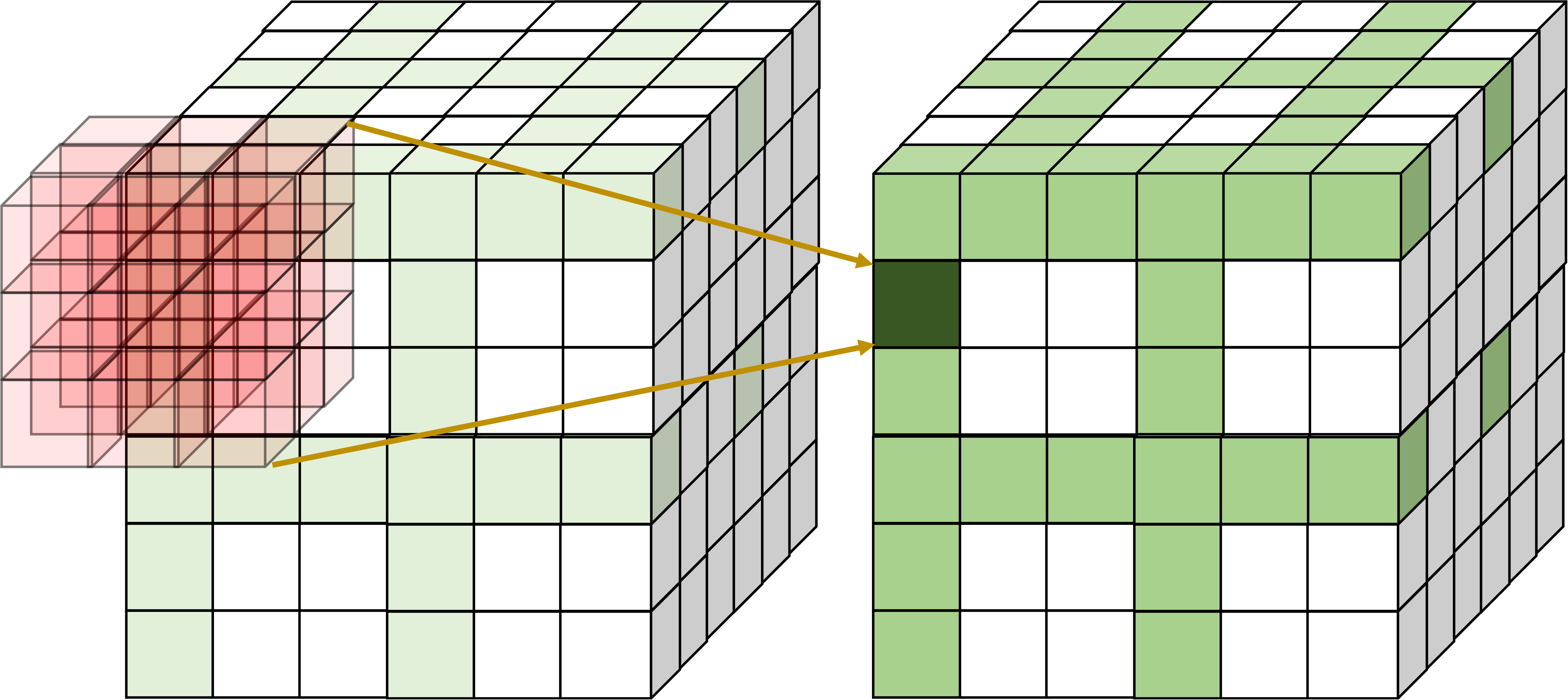
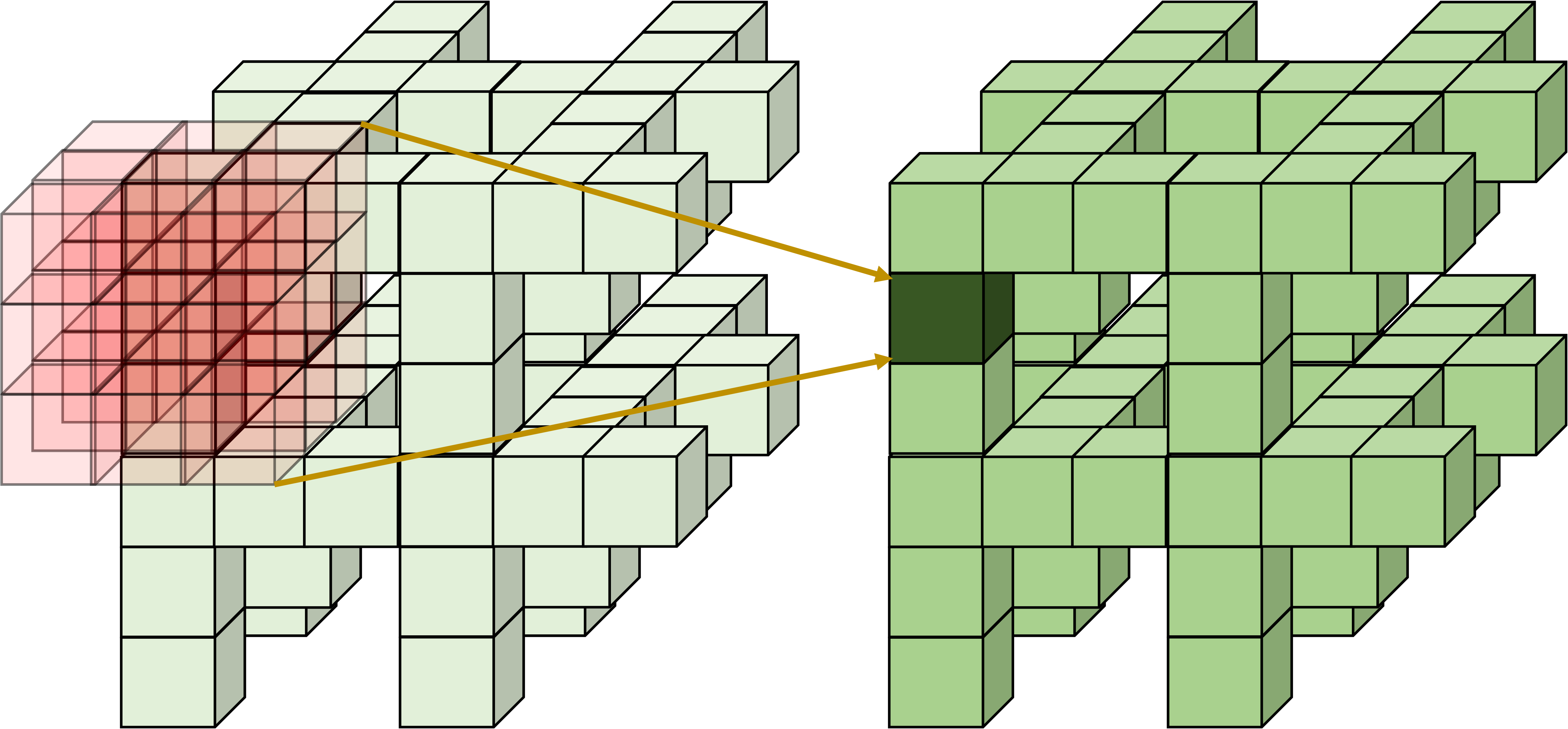
Figure 1: Differences between dense and sparse convolution with kernel size $3\times 3\times 3$. (a) dense convolution, (b) sparse convolution.

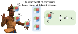
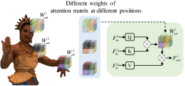
Figure 2: Differences between convolution and local attention weights at various voxels. (a) convolution in CNN. (b) local attention in Transformer.

$$\boldsymbol{f}_{\boldsymbol{u}}^{\text{out }}=\sum_{\boldsymbol{i}}\mathbf{W}_{\boldsymbol{i}}\boldsymbol{f}_{\boldsymbol{u}+\boldsymbol{i}}^{\text{in }},$$ (1)

where $\boldsymbol{f}_{\boldsymbol{u}}^{\text{out}}$ represents the output feature at 3D spatial coordinate $\boldsymbol{u}$ and $\boldsymbol{f}_{{\boldsymbol{u}}+{\boldsymbol{i}}}^{\mathrm{in\ }}$ represents the input feature at the position $\boldsymbol{u+i}$ , where $\boldsymbol{i}$ is an offset of $\boldsymbol{u}$ in 3D space. $\mathbf{W}_{\boldsymbol{i}}$ represents the convolution kernel weight corresponding to offset $\boldsymbol{i}$.

For spatial scale-invariant dense convolution, $\boldsymbol{i}$ is an offset selected from the list of offsets $\mathcal{V}^{3}(K)$ in a 3D hypercube with center $\boldsymbol{u}$, where $K$ is the size of one dimension of the convolution kernel. More intuitively, Fig. 1 illustrates the difference between sparse convolution and dense convolution. For a convolution operation with kernel size $3^{3}$, dense convolution stores both occupied and blank voxels. During the convolution, it acts on all 27 voxels covered by the convolution kernel. However, for spatial scale-invariant sparse convolution, $\boldsymbol{i}$ is an offset selected from the set of offsets $\mathcal{N}^{{3}}(\boldsymbol{u},\boldsymbol{C}^{\text{in}})$, which is defined as the set of offsets from the current center $\boldsymbol{u}$ that exists in the set $\boldsymbol{C}^{\text{in }}$. $\boldsymbol{C}^{\text{in}}$ are predefined input coordinates of sparse tensors that only include occupied voxels. As depicted in Fig. 1, sparse convolution only stores and acts on the occupied voxels, namely the 6 occupied voxels covered by the convolution kernel. In addition, sparse convolution does not perform convolution with empty voxels at the center. Compared with dense convolution, sparse convolution leads to significant savings in terms of memory cost and computational complexity, enabling the design of non-block compression models and more powerful compression networks for large-scale point clouds.

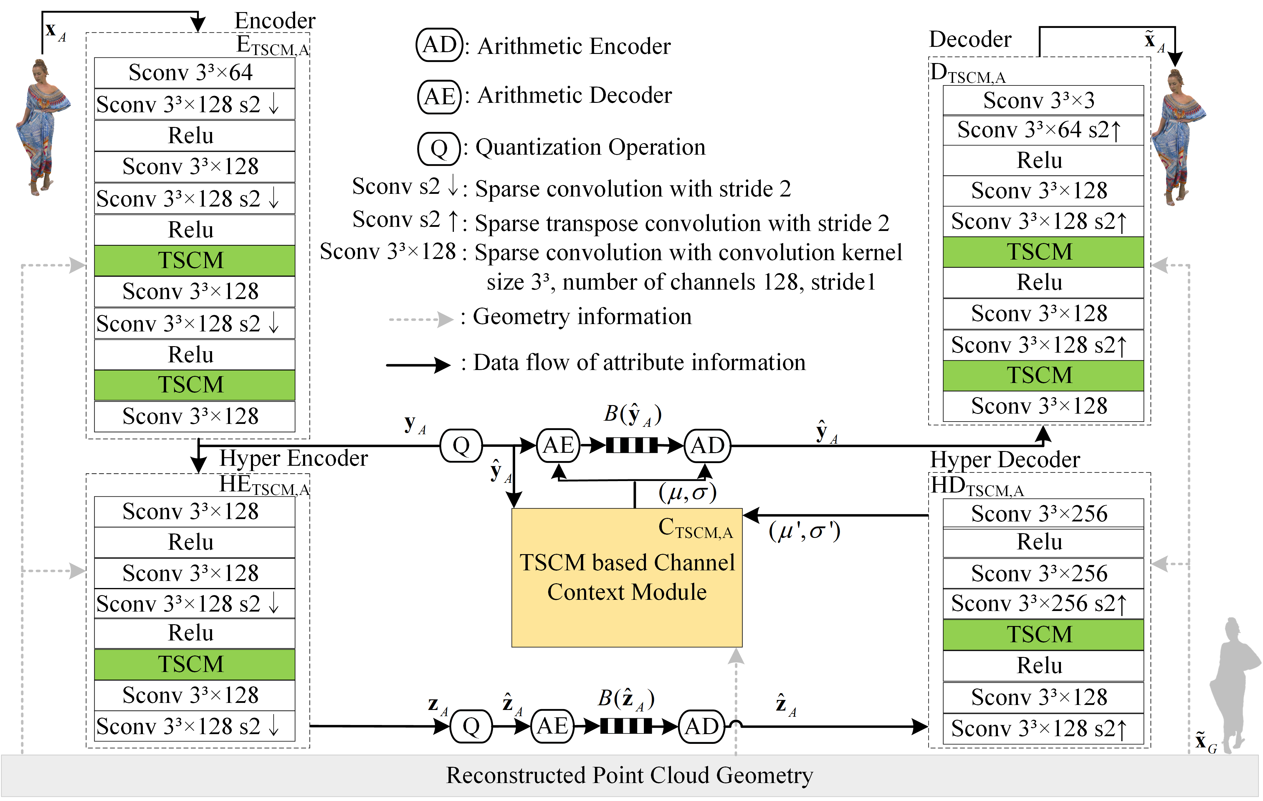
Figure 3: Framework of the proposed TSC-PCAC, where green and yellow rectangles are newly added TSCM and TSCM based channel context model.

III-A2 Importance of Local Attention

Fig. 2 shows the processing of the point cloud with the learned weights of the convolution kernel. Since there is only one set of weights in each convolution, it traverses the entire point cloud using a sliding convolution kernel to extract features, resulting in the learned convolution kernel being equally applied to different regions of the point cloud. Obviously, the properties of the regions/voxels vary from each other. Therefore, it is not the optimal solution to treat all voxels equally without considering the content of the regions. In contrast, the self-attention mechanism uses the input content to compute the attention matrix to model the dependencies of different voxels. As shown in Fig. 2, in a block, the local attention operator in transformers computes the attention weights of the input voxels with respect to other voxels, which are used to weight the input voxels to get the output so that the network is able to capture correlations between voxels. In this case, the correlations between voxels are captured using the self-attention mechanism to model the redundancy between voxels and reduce the bitrate for transmission by removing that redundancy. Moreover, in comparison to convolution, transformers utilize self-attention mechanisms to establish mutual dependencies between voxels, enhancing their capacity for stronger feature representation. However, transformers lack the capacity of effective inductive bias, which can compromise their generalization performance, particularly in the realm of 3D point cloud processing. Combining transformers with sparse convolution that has strong generalization capabilities can effectively alleviate the problem.

III-B Framework of the TSC-PCAC

Given a point cloud $\mathbf{x}_{pc}$, a learned point cloud compression framework to encode and decode $\mathbf{x}_{pc}$ can be expressed as

$$\begin{cases}\begin{aligned} &B(\hat{\mathbf{y}}_{pc})=AE(Q(E_{pc}(\mathbf{x}_{pc})))\\ &\tilde{\mathbf{x}}_{pc}=D_{pc}(AD(B(\hat{\mathbf{y}}_{pc})))\end{aligned}\end{cases},$$ (2)

where $E_{pc}(\cdot)$ and $D_{pc}(\cdot)$ represent the point cloud compression encoder and decoder, respectively. $AE(\cdot)$ and $AD(\cdot)$ respectively represent arithmetic encoder and arithmetic decoder. $\mathbf{x}_{pc}$ and $\tilde{\mathbf{x}}_{pc}$ represent the original point cloud and the reconstructed point cloud. $\hat{\mathbf{y}}_{pc}$ and $B(\hat{\mathbf{y}}_{pc})$ represent the compact latent representations after quantization and the bitstream containing the $\hat{\mathbf{y}}_{pc}$ information. $Q(\cdot)$ is quantization operation.

As point cloud $\mathbf{x}_{pc}$ consists of geometry $\mathbf{x}_{G}$ and attribute $\mathbf{x}_{A}$, i.e., $\mathbf{x}_{pc}=[\mathbf{x}_{A},\mathbf{x}_{G}]$, the geometry and attribute are sequentially compressed [2, 1], where attribute is coded after geometry and on the basis of the coded geometry. Thus, Eq.(2) is rewritten as

$$\begin{cases}\begin{aligned} &B(\hat{\mathbf{y}}_{G})=AE(Q(E_{G}(\mathbf{x}_{G})))\\ &\tilde{\mathbf{x}}_{G}=D_{G}(AD(B(\hat{\mathbf{y}}_{G})))\\ &B(\hat{\mathbf{y}}_{A})=AE(Q(E_{A}(\mathbf{x}_{A},\tilde{\mathbf{x}}_{G})))\\ &\tilde{\mathbf{x}}_{A}=D_{A}(AD(B(\hat{\mathbf{y}}_{A})),\tilde{\mathbf{x}}_{G})\end{aligned}\end{cases},$$ (3)

where $\tilde{\mathbf{x}}_{G}$ and $\tilde{\mathbf{x}}_{A}$ represent the reconstructed point cloud geometry and attribute. $\hat{\mathbf{y}}_{G}$ and $\hat{\mathbf{y}}_{A}$ represent the quantified latent representations of geometry and attribute. $E_{G}(\cdot)$ and $D_{G}(\cdot)$ represent point cloud geometry encoder and decoder. $E_{A}(\cdot)$ and $D_{A}(\cdot)$ represent the point cloud attribute encoder and decoder. $B(\hat{\mathbf{y}}_{G})$ and $B(\hat{\mathbf{y}}_{A})$ represent the bitstream containing the $\hat{\mathbf{y}}_{G}$ and $\hat{\mathbf{y}}_{A}$ information. Attribute $\mathbf{x}_{A}$ is on the basis of geometry ${\mathbf{x}}_{G}$, thus geometry is compressed before the attribute, and then the attribute is compressed with the reconstructed geometry information $\tilde{\mathbf{x}}_{G}$ as an input.

In this work, suppose that point cloud geometry has already been compressed, we focus on optimizing the point cloud attribute compression. Consequently, our goal is to optimize $E_{A}(\cdot)$ and $D_{A}(\cdot)$, as well as the entropy model required in arithmetic codec while encoding and decoding $\hat{\mathbf{y}}_{A}$. We propose an efficient TSC-PCAC framework based on the VAE, as shown in Fig. 3, in which TSCM and a TSCM based context module are proposed to adapt point cloud coding and improve the coding efficiency. The TSC-PCAC combines the inductive bias capabilities and memory-saving advantages of sparse convolution, and also leverages the ability of transformers in capturing correlations between voxels. The TSC-PCAC consists of a learning-based encoder, a decoder, and an entropy model, which can be represented as

$$\begin{cases}\begin{aligned} &B(\hat{\mathbf{y}}_{A})=AE(Q(E_{{TSCM},A}(\mathbf{x}_{A},\tilde{\mathbf{x}}_{G};\boldsymbol{\phi})))\\ &\tilde{\mathbf{x}}_{A}=D_{{TSCM},A}(AD(B(\hat{\mathbf{y}}_{A})),\tilde{\mathbf{x}}_{G};\boldsymbol{\theta})\\ &\{\boldsymbol{\mu},\boldsymbol{\sigma}\}=Entropy_{A}(\mathbf{y}_{A},\tilde{\mathbf{x}}_{G})\end{aligned}\end{cases},$$ (4)

where ${\mathbf{y}}_{A}$ represents the latent representations of attribute. $E_{{TSCM},A}(\cdot)$ and $D_{{TSCM},A}(\cdot)$ perform TSCM-optimized encoder and decoder in the end-to-end attribute coding with parameters $\boldsymbol{\phi}$ and $\boldsymbol{\theta}$, respectively. $Entropy_{A}(\cdot)$ represents the entropy model for the quantized latent representation of the attribute $\hat{\mathbf{y}}_{A}$. The mean $\boldsymbol{\mu}$ and scale $\boldsymbol{\sigma}$ estimated by the entropy model are used to construct the Laplace distribution $\mathcal{L}(\boldsymbol{\mu},\boldsymbol{\sigma})$ for the arithmetic codec. Specifically, the entropy model consists of a hyper-prior encoder-decoder and context module. In estimating the probability distribution of $\hat{\mathbf{y}}_{A}$, the initial mean and scale are firstly achieved by a hyper-prior encoder-decoder, and then refined by a context module. This can be represented as

$$\begin{cases}\begin{aligned} &B(\hat{\mathbf{z}}_{A})=AE(Q(HE_{{TSCM},A}\left(\mathbf{y}_{A},\tilde{\mathbf{x}}_{G};\boldsymbol{\phi}_{h}\right)))\\ &\{\boldsymbol{\mu^{\prime}},\boldsymbol{\sigma^{\prime}}\}=HD_{{TSCM},A}\left(AD(B(\hat{\mathbf{z}}_{A})),\tilde{\mathbf{x}}_{G};\boldsymbol{\theta}_{h}\right)\\ &\{\boldsymbol{\mu},\boldsymbol{\sigma}\}=C_{{TSCM,A}}\left(\boldsymbol{\mu^{\prime}},\boldsymbol{\sigma^{\prime}},\hat{\mathbf{y}}_{A},\tilde{\mathbf{x}}_{G};\boldsymbol{\theta}_{c}\right)\end{aligned}\end{cases},$$ (5)

where $B(\hat{\mathbf{z}}_{A})$ represent the bitstream containing the quantized hyperprior representations $\hat{\mathbf{z}}_{A}$ information. $HE_{{TSCM},A}(\cdot)$ and $HD_{{TSCM},A}(\cdot)$ represent the hyperprior encoder with parameters $\boldsymbol{\phi}_{h}$ and the hyperprior decoder with parameters $\boldsymbol{\theta}_{h}$. $\boldsymbol{\mu^{\prime}}$ and $\boldsymbol{\sigma^{\prime}}$ represent initial mean and scale of $\hat{\mathbf{y}}$. $C_{{TSCM},A}$ denotes the channel context module with parameters $\boldsymbol{\theta}_{c}$. TSCM based channel context module is used to establish relationships between channels, providing contextual information and achieving higher compression ratios.

To enhance the network’s ability to allocate more importance to voxels with higher relevance, achieving reduction redundancy of point cloud and obtaining a compact representation, four TSCM blocks are placed in the encoder and decoder. Specifically, due to memory constraints, TSCM blocks are only used on the lowest two scales of the encoder and decoder. Similarly, one TSCM block is employed in both the hyper-prior encoder and decoder. Since the attribute is attached to geometry, the geometry information is indeed utilized in the entire process of attribute coding. For simplicity, geometry variables are not explicitly indicated in subsequent diagrams.

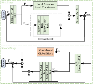
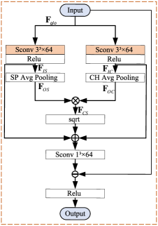
Figure 4: The structure of the TSCM and its key module. (a) TSCM, (b) Voxel-based Global Block. The ‘split’ operation performs channel-wise splitting. ‘SP Avg Pooling’ refers to spatial average pooling, which applies global pooling operation across spatial dimensions, and ‘CH Avg Pooling’ refers to channel-wise average pooling, which applies global pooling operation across channel dimensions.

III-C Architecture of TSCM

Transformers, which model the correlations dependencies between voxels through the self-attention mechanism, have the potential to enable the network to focus on voxels of higher relevance, but it may be deeply affected by the generalization ability. Convolution, on the other hand, has a strong inductive bias and can achieve excellent generalization ability. Combining convolution and transformer can gain their advantages. However, when the transformer is used to process large-scale color point clouds (containing millions of points), the memory cost of global attention becomes prohibitive. Using a transformer with local attention is a solution. However, compared to global attention, local attention greatly reduces the receptive field, making it hard to capture long-range dependencies. Therefore, we introduce global blocks to increase the receptive field of the network so that features have a global receptive field. To combine the advantages of all, we propose a two-stage TSCM, which consists of local attention based transformer [37], residual block, and voxel-based global block. Fig. 4 shows the framework of the proposed TSCM.

In the first stage, residual block and local attention based transformer are utilized to extract local features. To fuse the strengths of these features, we adopt a dual-branch structure, first extracting them separately and then using them jointly by concatenating. Specifically, an input $\mathbf{F}_{{in}}\in\mathbb{R}^{N\times 128}$ performs sparse convolution with a kernel size of 1 and splits along the channel dimension, resulting in $\mathbf{F}_{{att}}\in\mathbb{R}^{N\times 64}$ and $\mathbf{F}_{{cnn}1}\in\mathbb{R}^{N\times 64}$. They are used as inputs for the local attention-based transformer and residual block, respectively. The output is then concatenated to restore the feature channel to the original dimension, i.e., 128. This fusion combines both types of features to form local features $\mathbf{F}_{{out}1}\in\mathbb{R}^{N\times 128}$ with dual capabilities: capturing interdependencies among voxels and effective inductive bias. These features serve as the output of the first stage and the input of the second stage.

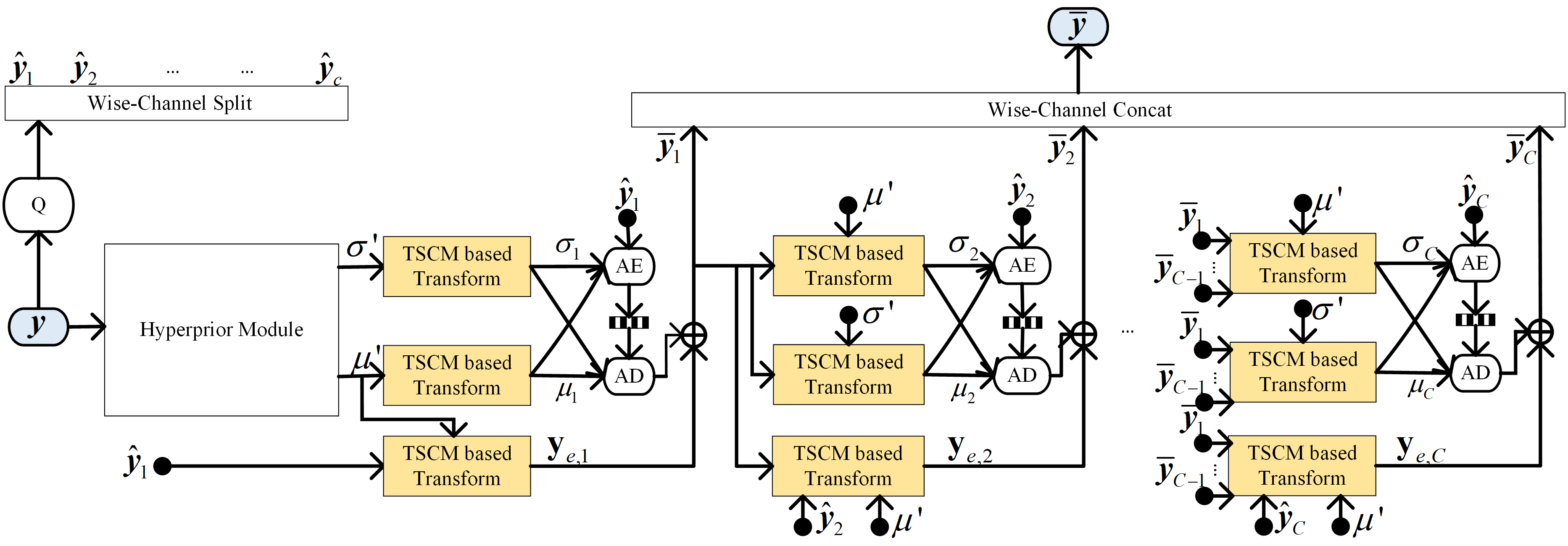
Figure 5: Detailed structure of the proposed TSCM based channel context module. (a) channel context module, (b) TSCM based transform.

In the second stage, to alleviate the computational and memory constraints and achieve the global features, the residual block and the global block are employed. The global block is inspired by the approach presented in [38], which uses linear layers and global pooling to extract global features and sharpen them. To further capture spatial neighboring redundancy, we replaced the linear layer with convolutional layers. This modified block is named the voxel-based global block. Specifically, similar to the first stage, $\mathbf{F}_{{glo}}\in\mathbb{R}^{N\times 64}$ and $\mathbf{F}_{{cnn}2}\in\mathbb{R}^{N\times 64}$ are obtained and served as input to the voxel-based global block and residual block, respectively. The voxel-based global block is shown in Fig. 4. It utilizes global pooling to extract global spatial features $\mathbf{F}_{{OS}}\in\mathbb{R}^{1\times 64}$ and global channel features $\mathbf{F}_{{OC}}\in\mathbb{R}^{N\times 1}$. $\mathbf{F}_{{OC}}$ and $\mathbf{F}_{{OS}}$ undergo matrix multiplication to obtain global spatial-channel features $\mathbf{F}_{{CS}}\in\mathbb{R}^{N\times 64}$. Subsequently, the global spatial-channel features are subtracted from the input features of voxel-based global block $\mathbf{F}_{{glo}}$ to obtain sharpened global spatial-channel features. The output of the voxel-based global block and residual block are concatenated to restore the feature channel to the original dimension. This fusion combines both types of features to form global features with a large receptive field and inductive bias capabilities.

In TSCM, the integration of these two stages effectively captures both global and local inter-point relevance for reducing data redundancy. The utilization of the residual block and the transformer with local self-attention enables the extraction of local features and correlations. In addition, the global features are obtained through channel and spatial pooling within voxel-based global blocks. Consequently, the output features of TSCM are represented as $\mathbf{F}_{\text{out}}\in\mathbb{R}^{N\times 128}$.

III-D TSCM based Channel Context Module

In the Sparse-PCAC, the context module is a per-voxel context network, which processes voxels sequentially. While dealing with large-scale point clouds, this sequential processing leads to extremely high encoding and decoding delays. We propose a TSCM based channel context module to improve the network prediction probability distribution by constructing contextual information over quantized latent representations. Features are processed sequentially along the channel dimension in the channel context module.

The architecture of the proposed TSCM based channel context module is illustrated in Fig. 5, where the hyper-prior module is detailed in Fig. 3. $\hat{\mathbf{y}}_{i}$ represents the latent representation of the i-th quantized slice, while $\overline{y}_{i}$ represents the latent representation of the i-th slice with the addition of quantization error estimation, where $i\in{\{1,2,3,\ldots,C\}}$. $C$ represents the number of equal divisions in the channel. Besides the mean and scale, we also employ a module to predict quantization error. Specifically, the channel context module processes each slice serially by dividing the quantized latent representation $\hat{\mathbf{y}}$ proportionally into slices along the channel. The mean prediction for each slice is then conditioned on the previously decoded slices and the initial mean. The same process is applied to the scale. Since the obtained probability distribution can decode the current slice, the quantization error prediction can utilize information from the decoded current slice. It is worth noting that the network architecture for the mean, scale, and quantization error prediction is identical. We use the term ‘TSCM based Transform’ for different cases. The details are depicted in Fig. 5, where all inputs are concatenated and processed through a sparse convolutional network with TSCM blocks.

Due to the computational complexity, we reduce the number of feature channels to 32, followed by the TSCM. The mathematical expressions for obtaining the scale, mean, and quantization error can be formulated as

$$\begin{cases}\begin{aligned} \boldsymbol{\sigma}_{i}&=f_{\text{TSCM\_T }}\left(\overline{\mathbf{y}}_{<i},\boldsymbol{\sigma}^{\prime};\boldsymbol{\theta}_{\sigma,i}\right)\\ \boldsymbol{\mu}_{i}&=f_{\text{TSCM\_T }}\left(\overline{\mathbf{y}}_{<i},\boldsymbol{\mu}^{\prime};\boldsymbol{\theta}_{\mu,i}\right)\\ {\mathbf{y}}_{e,i}&=f_{\text{TSCM\_T }}\left(\overline{\mathbf{y}}_{<i},\hat{\mathbf{y}}_{i},\boldsymbol{\mu}^{\prime};\boldsymbol{\theta}_{y,i}\right)\end{aligned}\end{cases},$$ (6)

where $\boldsymbol{\mu}_{i}$ and $\boldsymbol{\sigma}_{i}$ represent the refined mean and scale of $\hat{\mathbf{y}}_{i}$. ${\mathbf{y}}_{e,i}$ is the estimated quantization error. $\overline{\mathbf{y}}_{i}$ denotes the refined latent representation of group $i$, i.e., $\overline{\mathbf{y}}_{i}={\mathbf{y}}_{e,i}+\hat{\mathbf{y}}_{i}$. $\overline{\mathbf{y}}_{<i}$ indicates a set of $\overline{\mathbf{y}}_{j}$ where $j$ is smaller than $i$, $\overline{\mathbf{y}}_{<i}=\left\{\overline{\mathbf{y}}_{1},\overline{\mathbf{y}}_{2},\ldots,\overline{\mathbf{y}}_{i-1}\right\}$. $f_{\text{TSCM\_T }}(\cdot)$ performs the ‘TSCM based Transform’, with different parameters for predicting the scale, mean and quantization error of different slices, which are $\boldsymbol{\theta}_{\sigma,i}$, $\boldsymbol{\theta}_{\mu,i}$, and $\boldsymbol{\theta}_{y,i}$, respectively. The mean $\boldsymbol{\mu}_{i}$ and scale $\boldsymbol{\sigma}_{i}$ predicted for $i$ group are utilized for entropy encoding and decoding of the current group’s $\hat{\mathbf{y}}_{i}$. The quantization error $\mathbf{y}_{e,i}$ predicted for each group is then employed to refine $\hat{\mathbf{y}}_{i}$. Based on Eq. 6 and Fig.5, the mean $\boldsymbol{\mu}_{i}$, scale $\boldsymbol{\sigma}_{i}$, and quantization error ${\mathbf{y}}_{e,i}$ can be predicted by the TSCM based transform, which improves the channel context module in entropy coding.

III-E Loss Function

The overall objective of point cloud compression is to minimize the distortion of the reconstructed point cloud at a given bitrate constraint. The objective of color point cloud compression is to minimize

$$\begin{gathered}L=R_{A}(\hat{\mathbf{y}}_{A})+R_{G}(\hat{\mathbf{y}}_{G})+{\lambda_{A}}D_{A}(\mathbf{x}_{A},\tilde{\mathbf{x}}_{A})+{\lambda_{G}}D_{G}(\mathbf{x}_{G},\tilde{\mathbf{x}}_{G}),\end{gathered}$$ (7)

where $D_{A}(\cdot)$ and $D_{G}(\cdot)$ are distortion measurements, and in this paper, $D_{A}(\cdot)$ is Mean Squared Error (MSE) loss in the YUV color space. $R_{A}(\hat{\mathbf{y}}_{A})$ and $R_{G}(\hat{\mathbf{y}}_{G})$ represent the bitrate required for transmitting the quantized attribute and geometry latent representations, $\hat{\mathbf{y}}_{A}$ and $\hat{\mathbf{y}}_{G}$. The trade-off between distortion and bitrate is controlled by $\lambda_{A}$ and $\lambda_{G}$. Furthermore, in this paper, we focus on attribute coding for point clouds. Therefore, assuming the geometry information is shared and fixed at the encoder and decoder sides, the objective for attribute coding is simplified to minimize

$$L_{A}=R_{A}(\hat{\mathbf{y}}_{A})+R_{A}(\hat{\mathbf{z}}_{A})+\lambda_{A}D_{A}(\mathbf{x}_{A},\tilde{\mathbf{x}}_{A}).$$ (8)

Due to the hyper-codec, the total bit rate of attribute consists of the bit rate of $\hat{\mathbf{z}}_{A}$, and $\hat{\mathbf{y}}_{A}$, i.e., $R_{A}(\hat{\mathbf{y}}_{A})+R_{A}(\hat{\mathbf{z}}_{A})$.

IV Experimental Results and Analyses

IV-A Experimental Settings

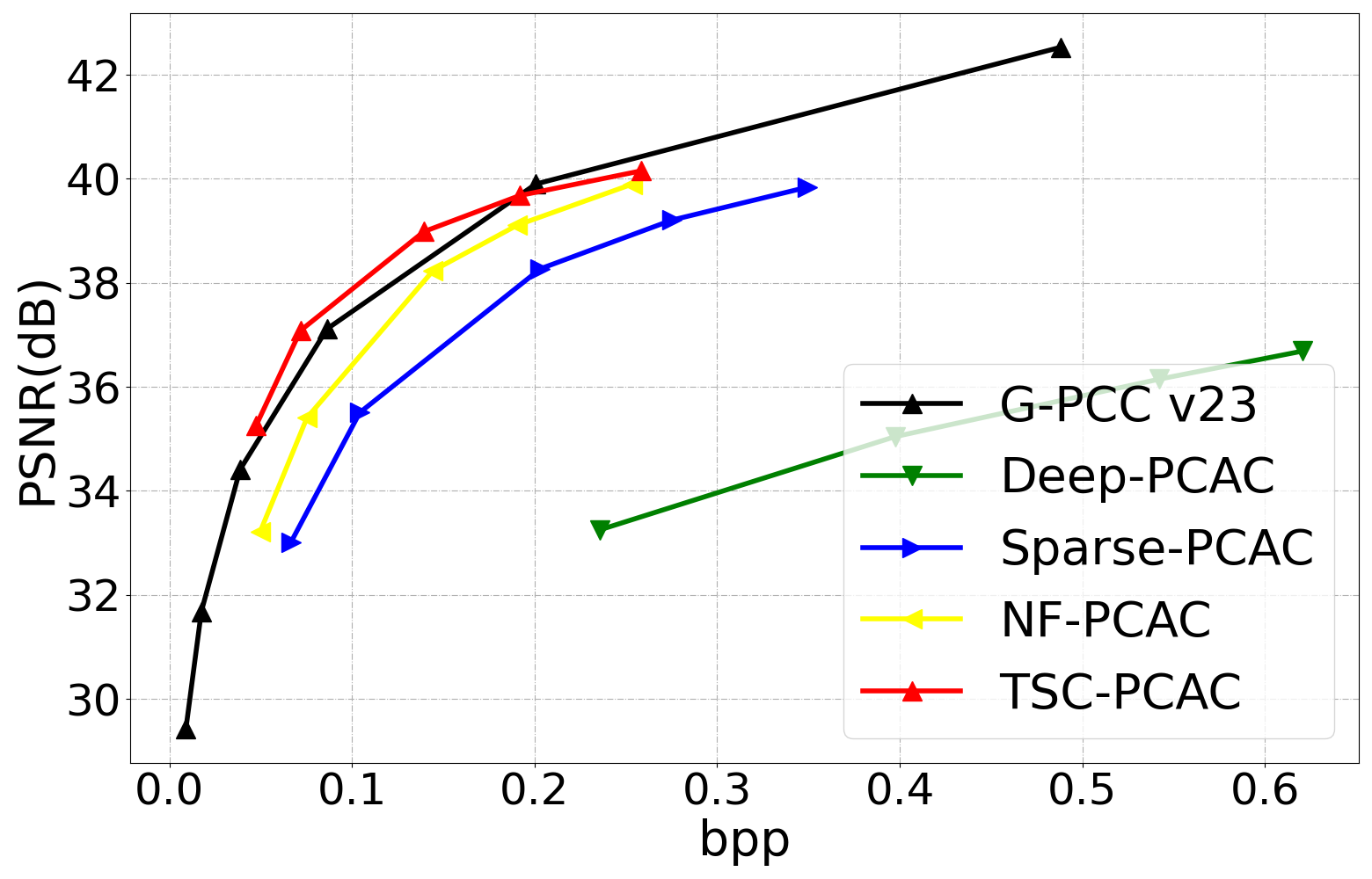
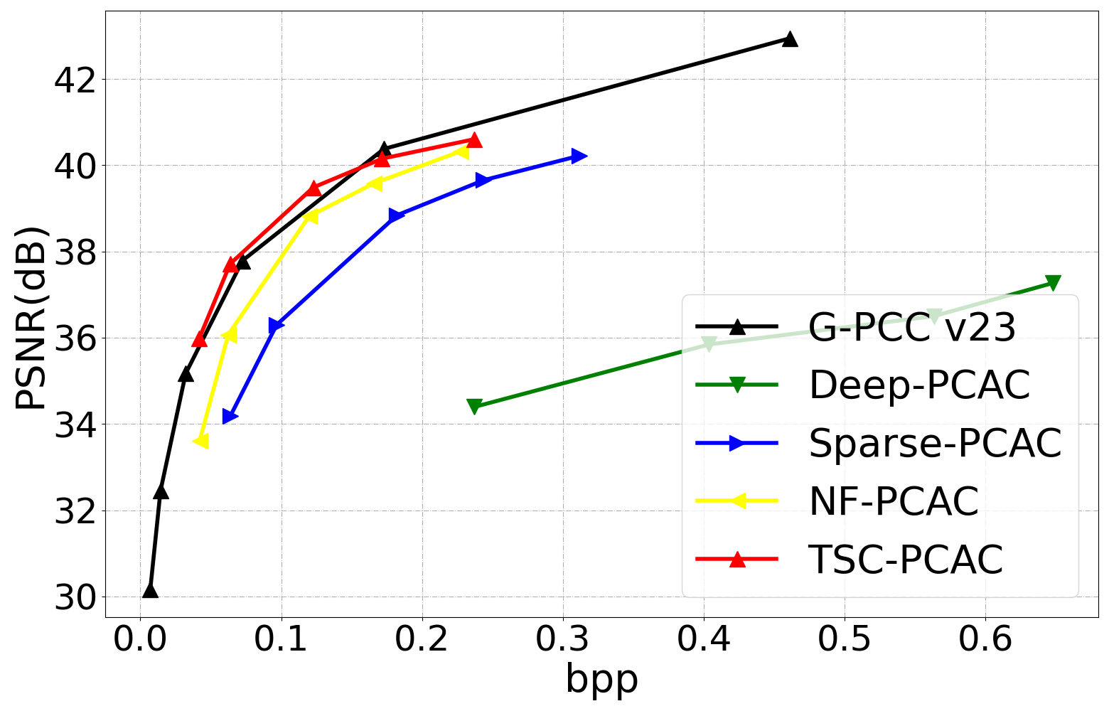
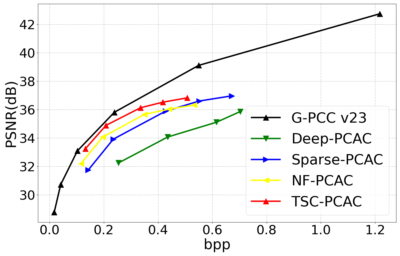
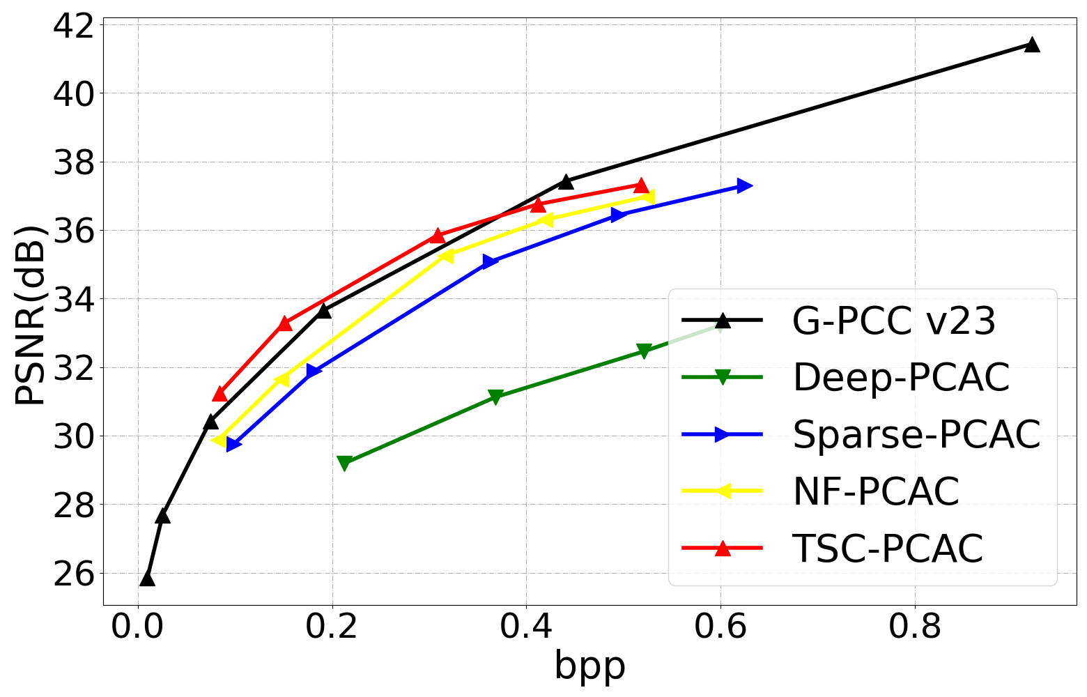
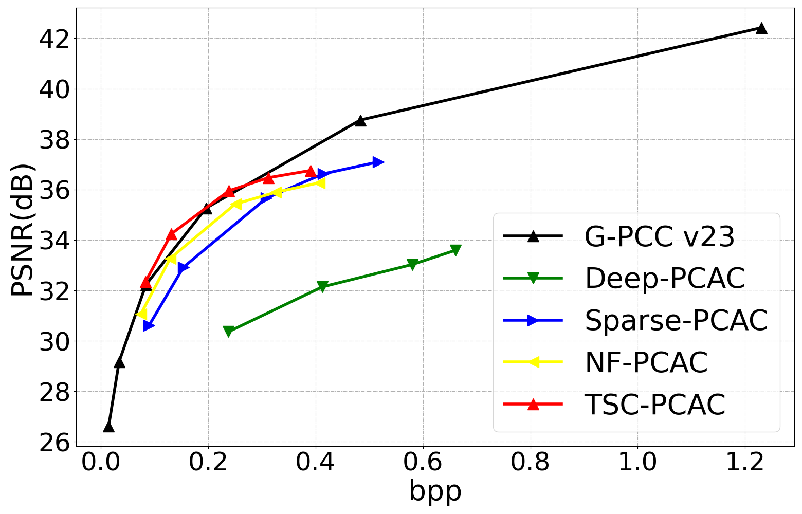
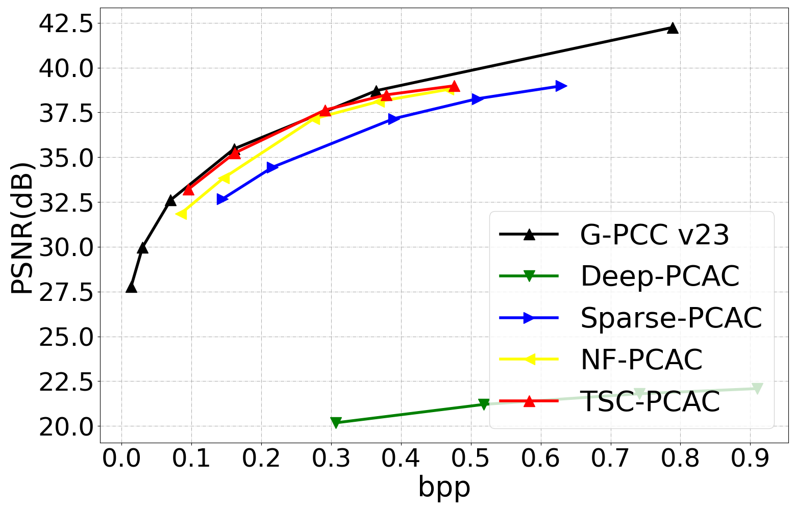
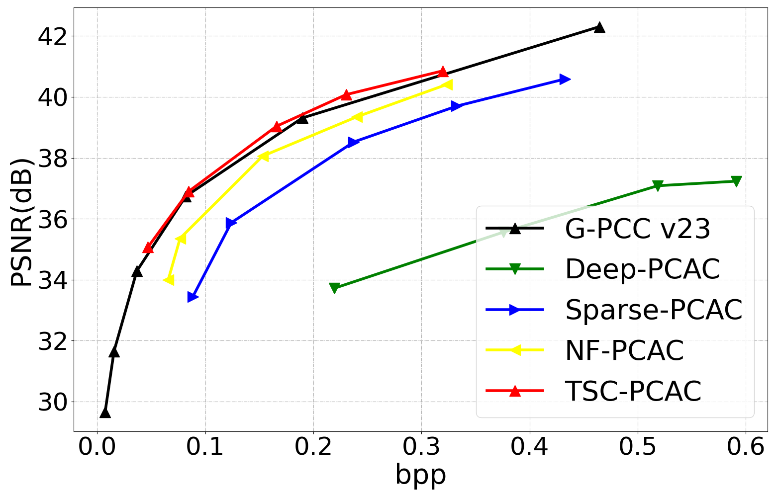
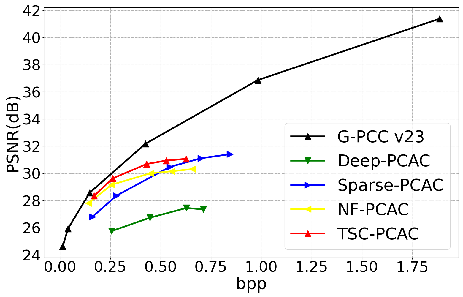
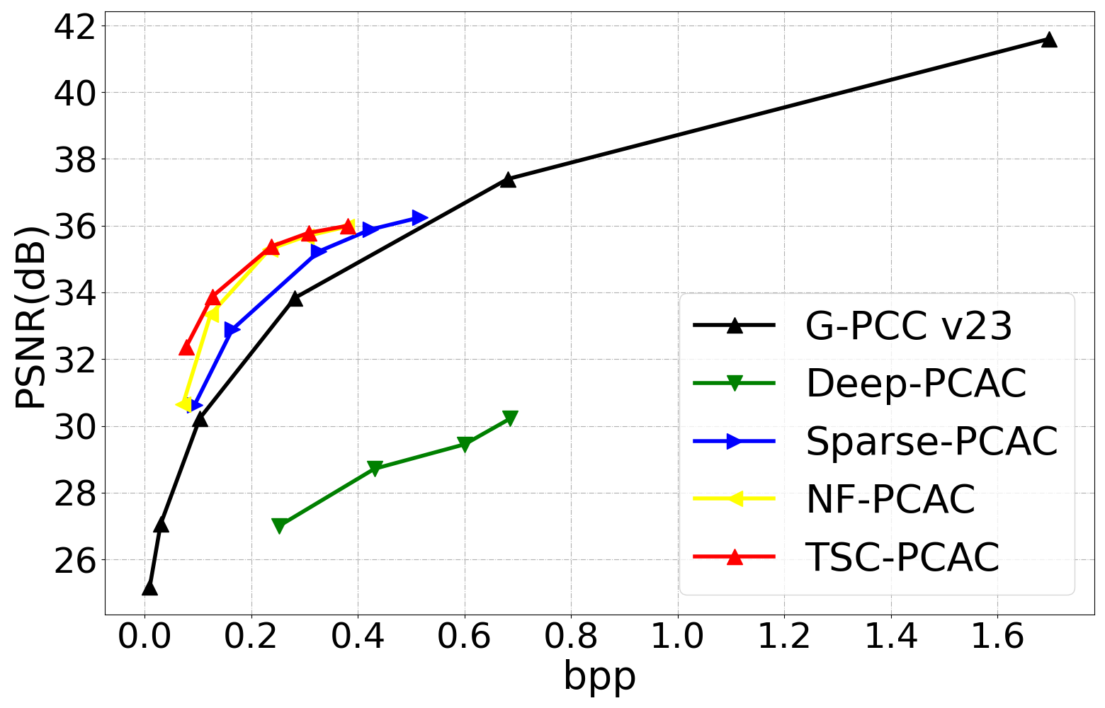
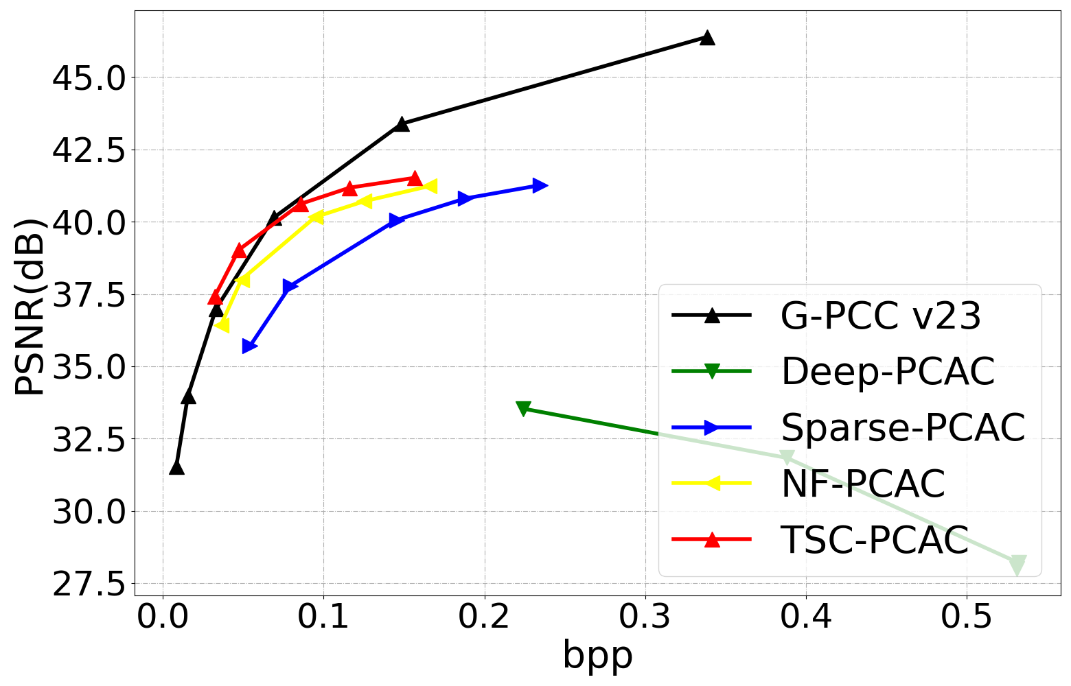
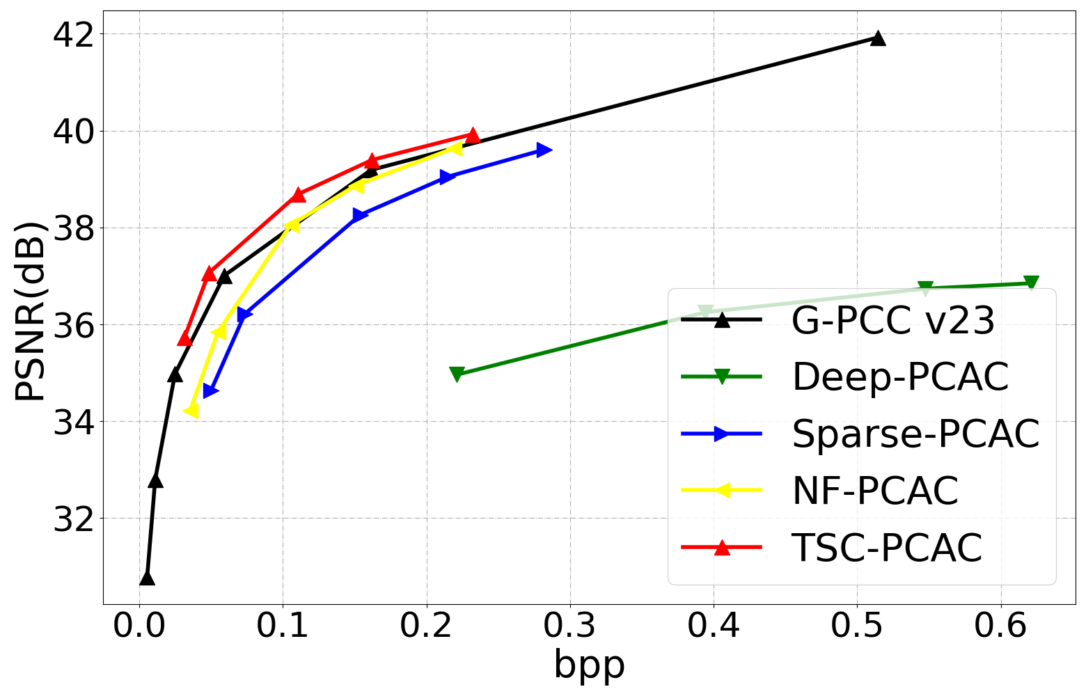
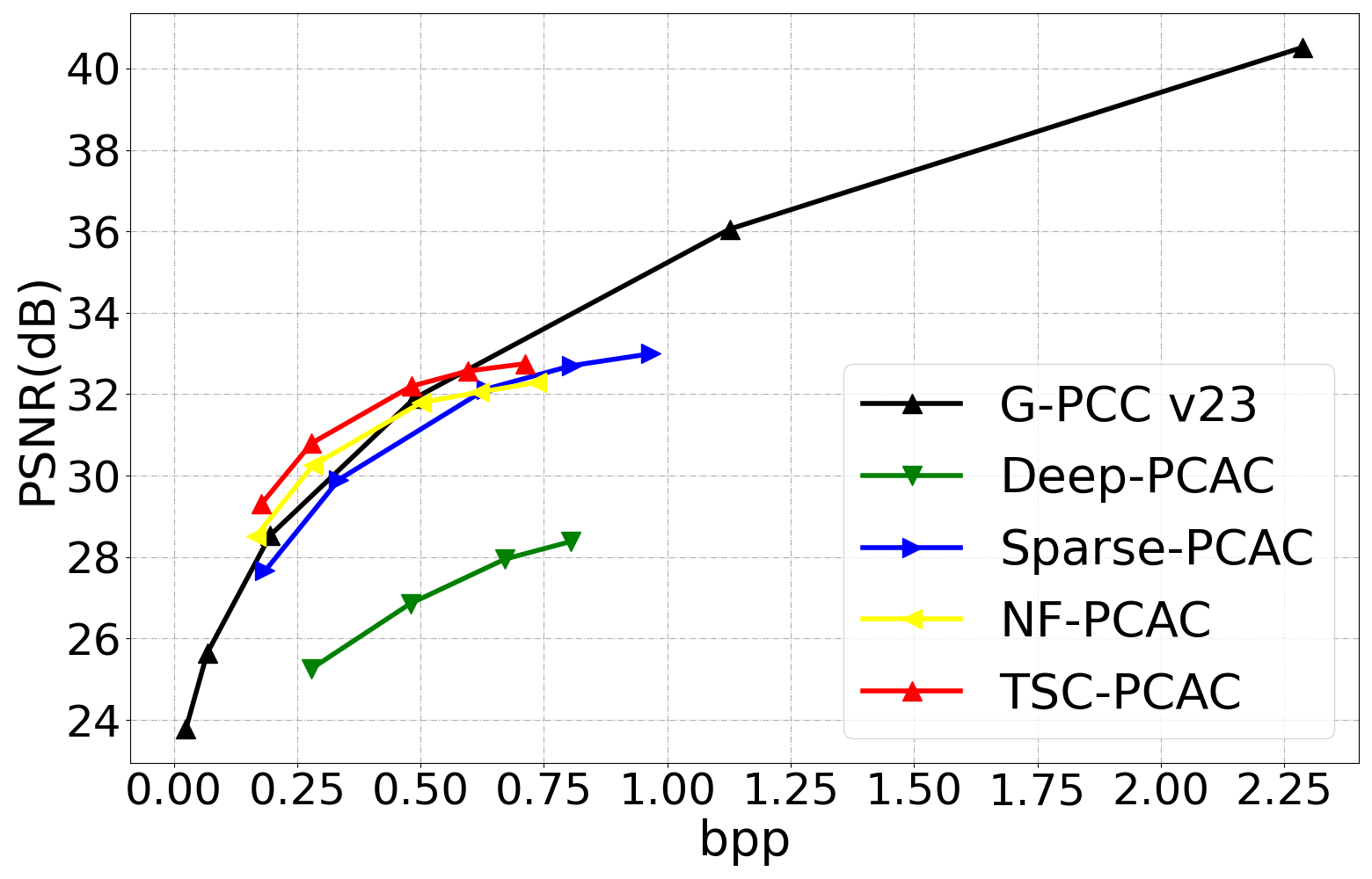
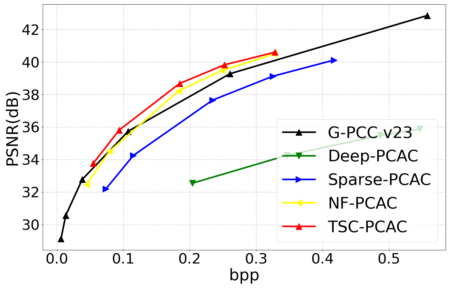
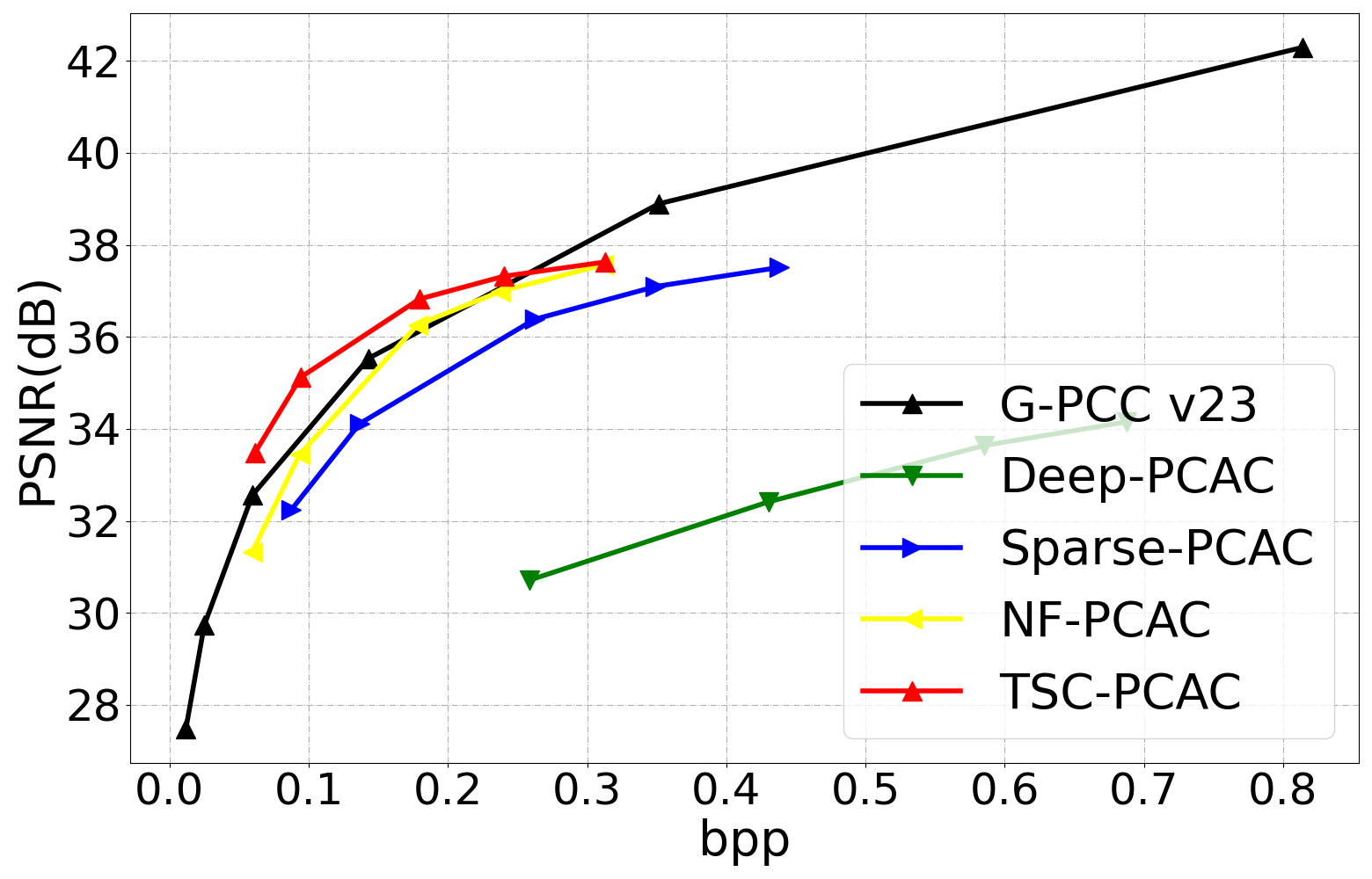
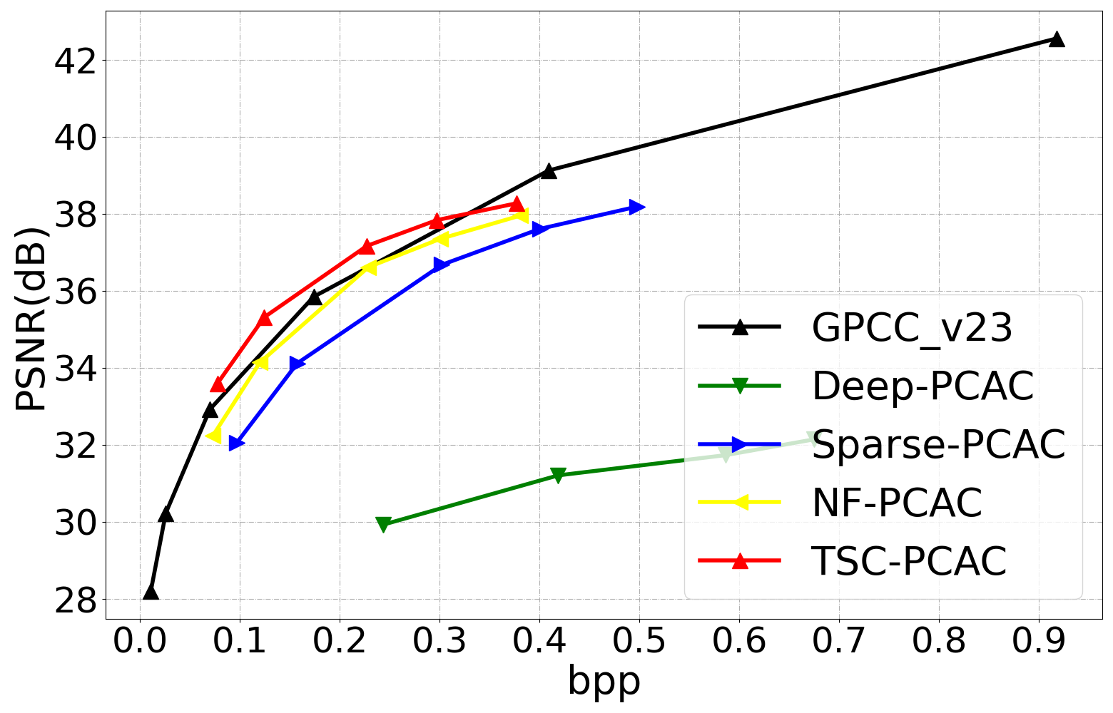
Figure 6: RD curves of the TSC-PCAC, Sparse-PCAC, Deep-PCAC, NF-PCAC and G-PCC for different point clouds. (a) Dancer, (b) Basketball Player, (c) Redandblack, (d) Soldier, (e) Phil, (f) Rafa, (g) Sir Frederick, (h) Boxer, (i) Thaidancer, (j) Andrew*, (k) Sarah*, (l) Exercise*, (m) Longdress*, (n) Loot*, (o) Model*, (p) Average*.

TABLE I: BD-BR and BD-PSNR of TSC-PCAC against the state-of-the-art.

PC	TSC-PCAC vs Sparse-PCAC		TSC-PCAC vs NF-PCAC		TSC-PCAC vs GPCC v23
	BD-BR-Y(%)	BD-PSNR-Y(dB)	BD-BR-Y(%)	BD-PSNR-Y(dB)	BD-BR-Y(%)	BD-PSNR-Y(dB)
Soldier	-35.09	1.73	-24.96	1.10	-8.08	0.22
Redandblack	-30.12	1.17	-19.13	0.59	22.44	-0.83
Dancer	-49.11	2.35	-29.61	1.25	-9.30	0.26
Basketball Player	-50.14	2.18	-25.68	1.04	-3.72	0.06
Phil	-33.65	1.48	-22.05	0.77	-4.33	0.02
Boxer	-44.00	2.01	-23.97	0.85	-2.43	0.07
Thaidancer	-32.67	1.15	-19.54	0.54	28.01	-1.28
Rafa	-35.93	1.58	-12.85	0.47	18.75	-0.67
Sir Frederick	-35.47	1.78	-13.22	0.61	7.58	-0.31
Andrew*	-37.26	1.44	-9.44	0.34	-53.07	2.46
David*	-50.57	2.57	-21.52	0.82	-0.63	0.01
Exerciese*	-45.76	1.40	-30.18	0.94	-14.63	0.34
Longdress*	-30.87	1.24	-18.38	0.55	-21.43	0.62
Loot*	-39.88	2.19	-11.24	0.48	-14.39	0.58
Model*	-44.87	1.77	-24.91	1.02	-18.72	0.54
Sarah*	-54.00	2.39	-26.13	0.86	0.12	-0.30
Average	-36.62	1.66	-22.27	0.85	1.26	-0.11
Average*	-38.53	1.72	-21.30	0.80	-11.19	0.34

IV-A1 Coding Methods

Four point cloud compression methods were compared with the proposed TSC-PCAC, including Deep-PCAC [11], Sparse-PCAC [12], NF-PCAC [14] and the traditional method G-PCC, where the G-PCC versions used are v23. For a fair comparison, we retrained the Sparse-PCAC and NF-PCAC models according to the training conditions of TSC-PCAC. As for the Deep-PCAC model, since the authors have provided pre-trained models, we used them to obtain coding results. The G-PCC encoding settings were configured with default settings for dense point clouds and the attribute encoding mode was RAHT. Quantization Parameters (QP) followed the default settings of Common Test Conditions [39].

IV-A2 Quality Metrics

Peak Signal-to-Noise Ratio (PSNR) was used as the quality metric for distortion measurement [40], and the rate was measured in bit per point (bpp). We also used Bjøntegaard Delta bitrate (BD-BR) to evaluate the coding performance. Additionally, we used Bjøntegaard Delta PSNR (BD-PSNR) to compare the reconstruction quality of different codecs at the same rate [41]. It’s worth noting that the PSNR in the paper are all based on luminance component PSNR (Y-PSNR), and obtained under geometry lossless conditions.

IV-A3 Databases

The dataset utilized consists of 8iVFB [42], Owlii [43], 8iVSLF [44], Volograms [45], and MVUB [46]. We selected the Longdress, Loot, Exercise, Model, Andrew, Sarah, and David point cloud sequences for training, and selected Redandblack, Soldier, Basketball Player, Dancer, Thaidancer, Boxer, Rafa, Sir Frederick and Phil point cloud sequences for testing. Longdress, Loot, Soldier, and Redandblack are from 8iVFB. Andrew, Sarah, David, and Phil are from MVUB. Exercise, Model, Basketball Player and Dancer are from Owlii. Rafa and Sir Frederick are from Volograms. Thaidancer and Boxer are from 8iVSLF. For Boxer and Thaidancer, following [47], we quantified them to 10-bit. For Rafa and Sir Frederick, we sampled them from mesh data to dense colored point cloud sequences with a precision of 10-bit. For the sequences of MVUB, we used point cloud sequences with a precision of 10-bit.

IV-A4 Training Settings

To reduce the data volume and accelerate training, the point clouds are resampled. Specifically, for a point cloud with $N$ points, we first used farthest point sampling to obtain $K$ point cloud cluster centers, where $K=Ceil\left(\frac{N}{100000}\right)$. Then, we used the k-Nearest Neighbor (kNN) algorithm to cluster the surrounding 100,000 points for each of the $K$ cluster centers, creating smaller point clouds. Resampling was applied to the first 100 frames of each point cloud sequence in the training set to train the network. To further validate the compression performance, the remaining frames of each point cloud sequence are compressed, whose coding results were marked with $*$. It is worth noting that the point clouds in the testing set were not resampled. We set $\lambda_{A}$ as 400, 1000, 4000, 8000, and 16000 to realize different bitrate points. For efficient training, we first trained a model with $\lambda_{A}$ as 16000. Then, we used this model as a base and fine-tuned it for 50 epochs with a learning rate of $10^{-5}$ to obtain models under different values of $\lambda_{A}$. During the training, we found that it was easier to train the model without the channel context module first and then jointly train it. Considering the trade-off between compression performance and encoding/decoding time complexity, we set the number of channel divisions C in the channel context module as 8. As for the hyperparameters in CodedVTR, specifically the number of codebook elements, we followed the settings in [37] and set it to 24. All the experiments were conducted on a workstation with an Intel Core i9-10900 CPU and an NVIDIA GeForce RTX 3090 GPU.

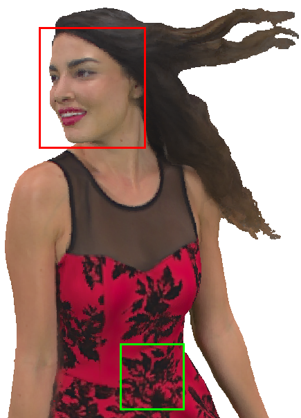
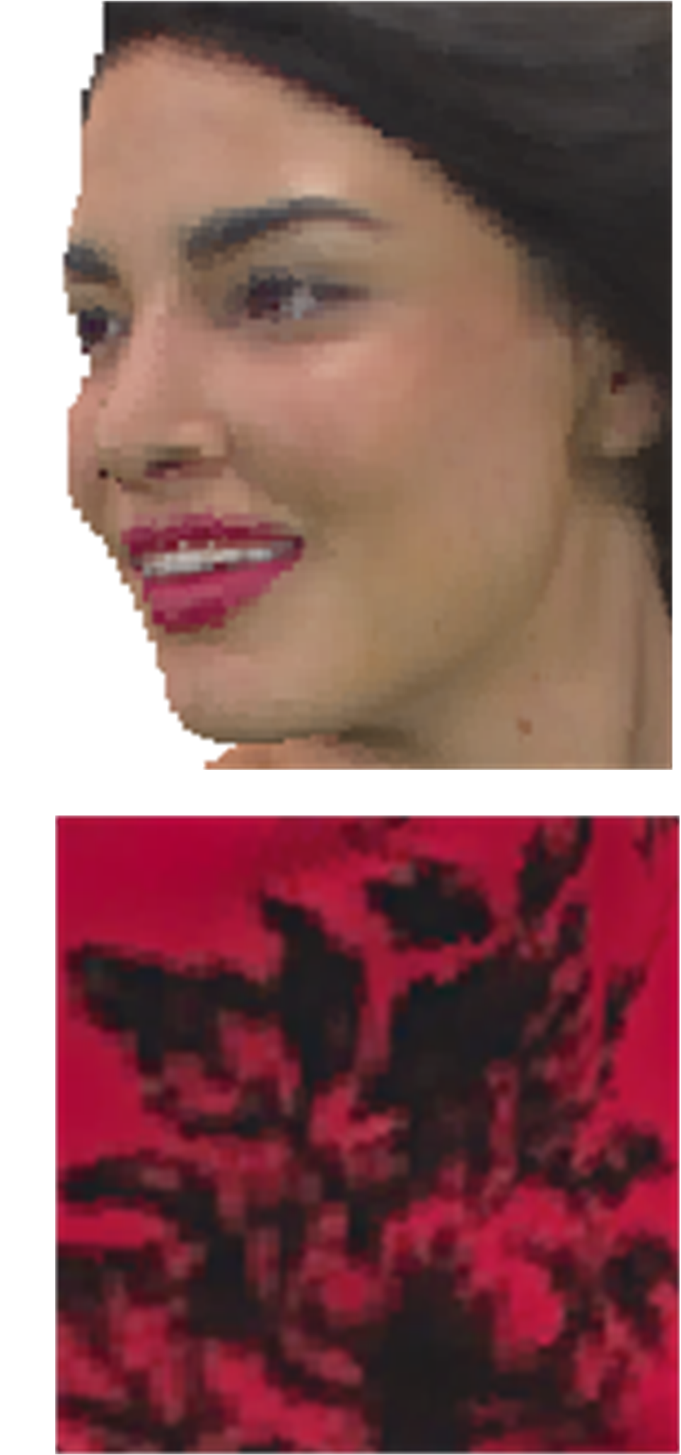
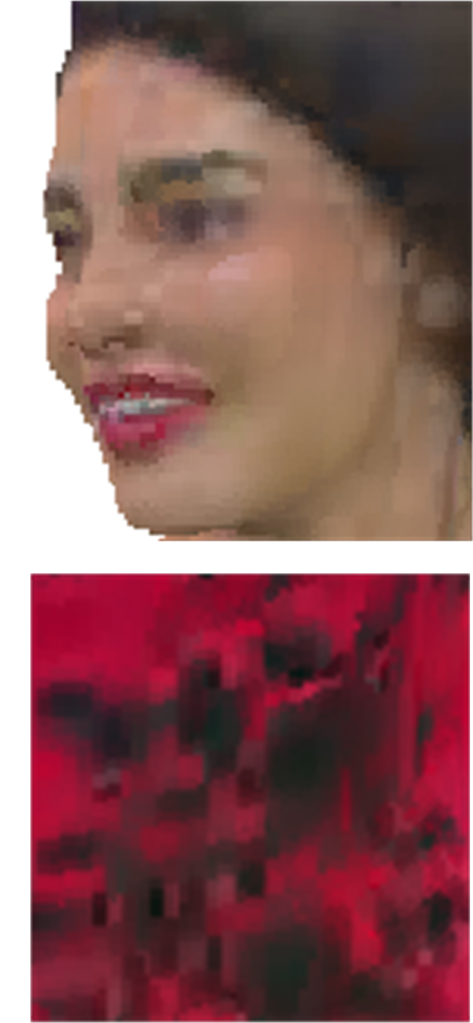
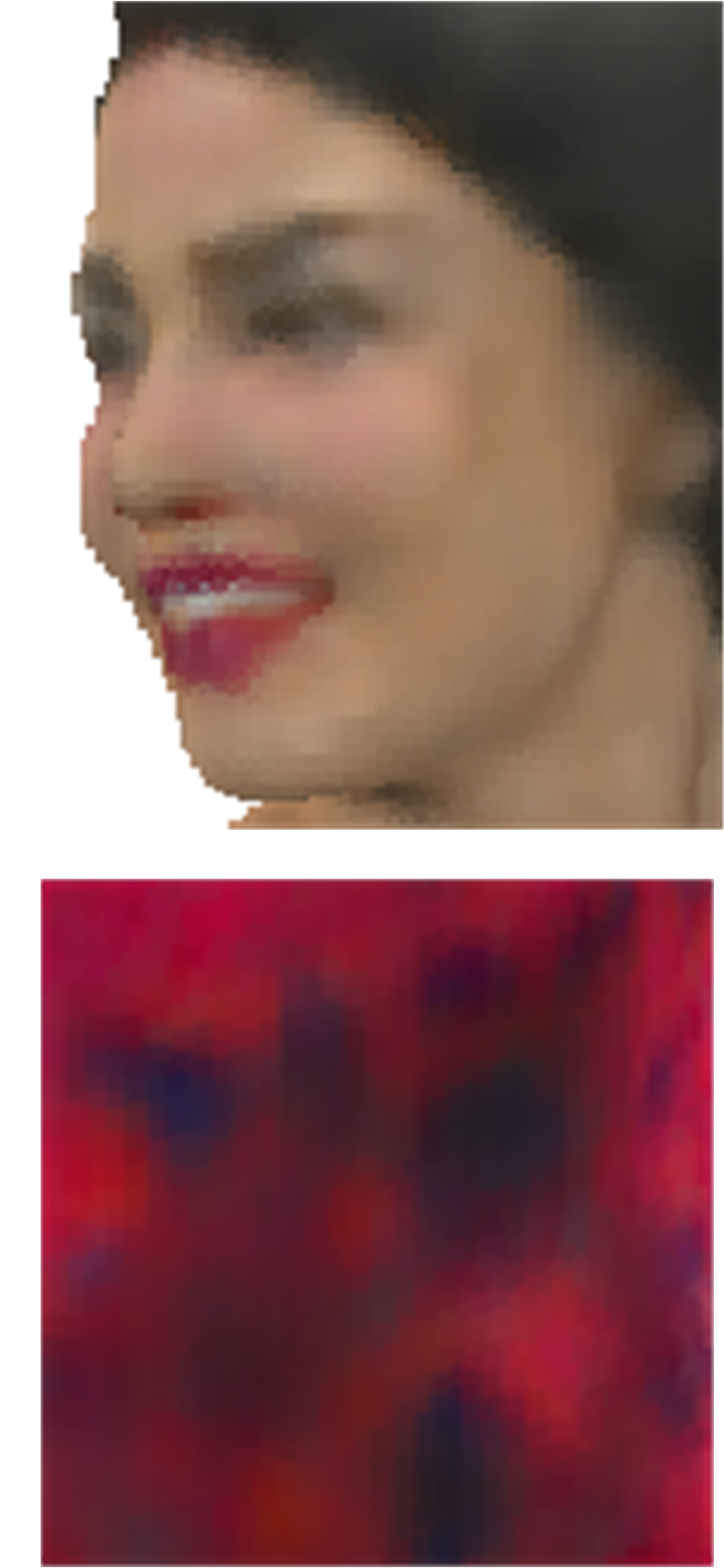
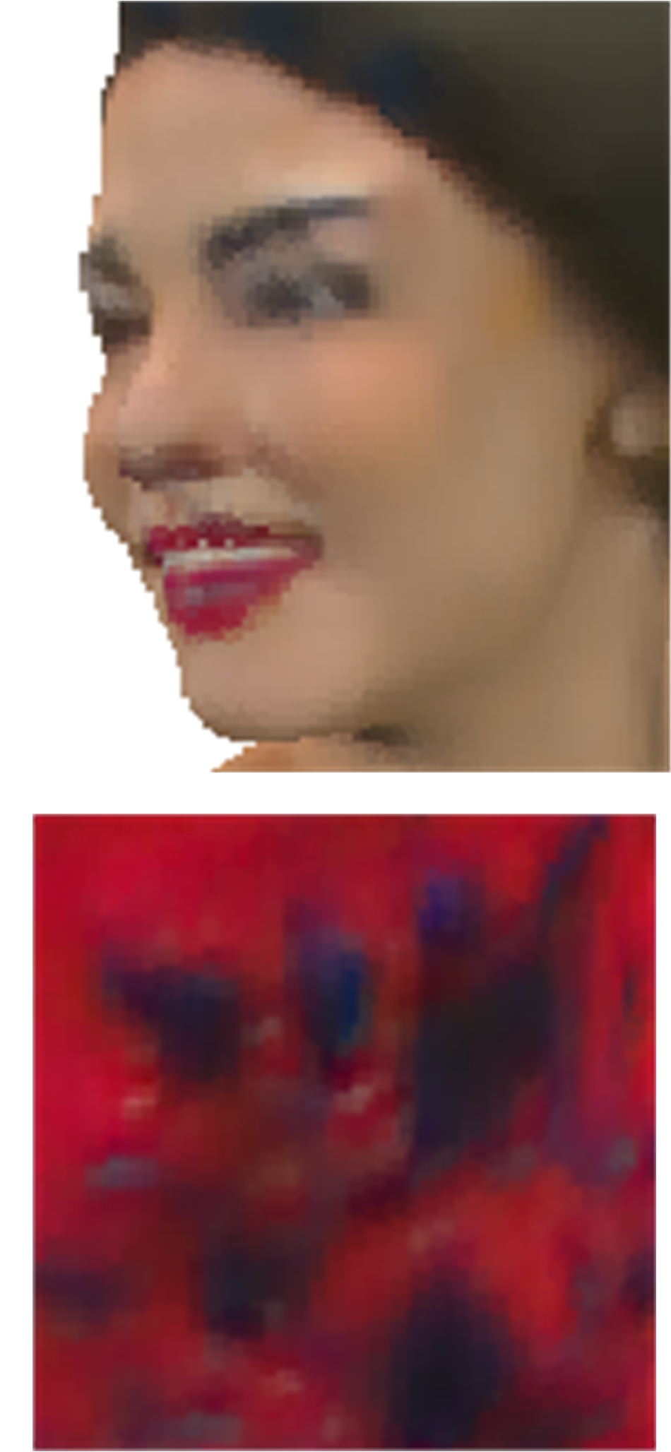
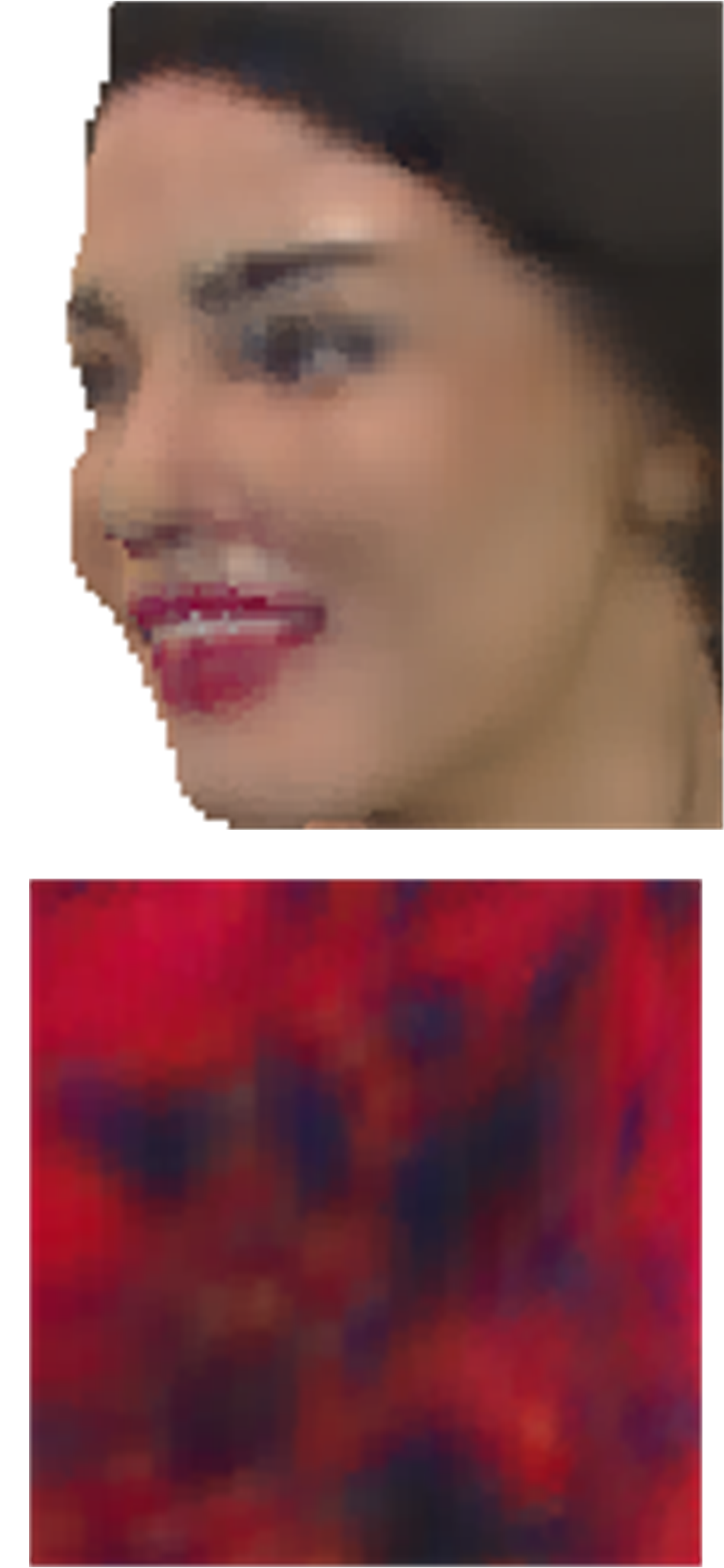
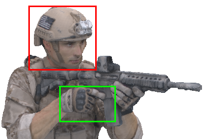
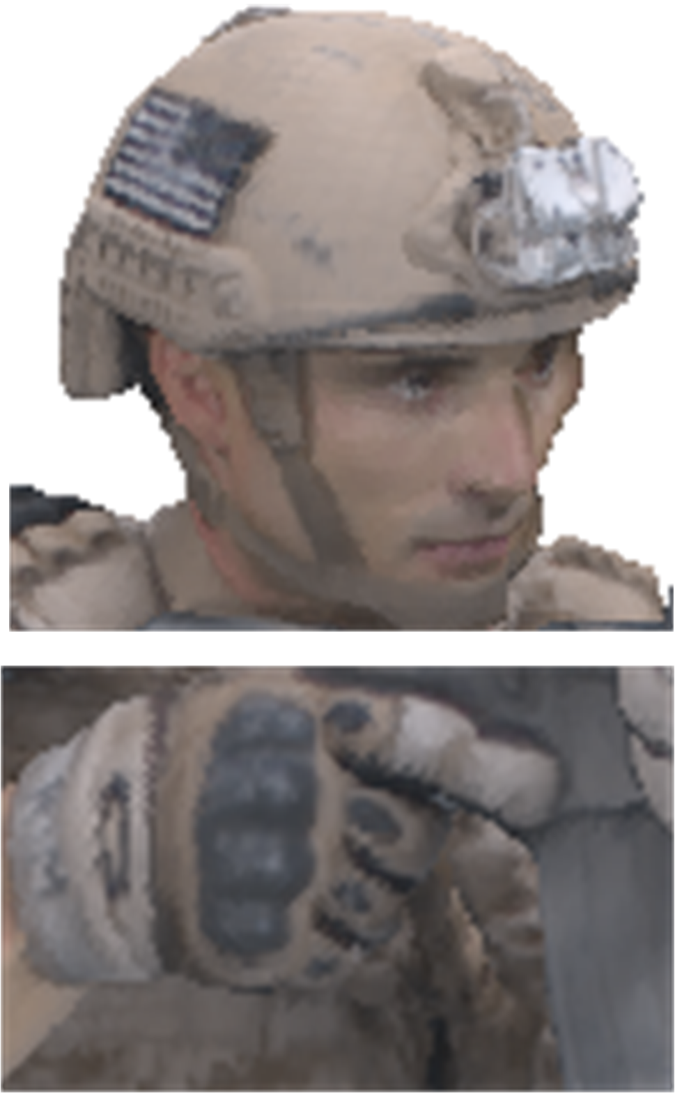
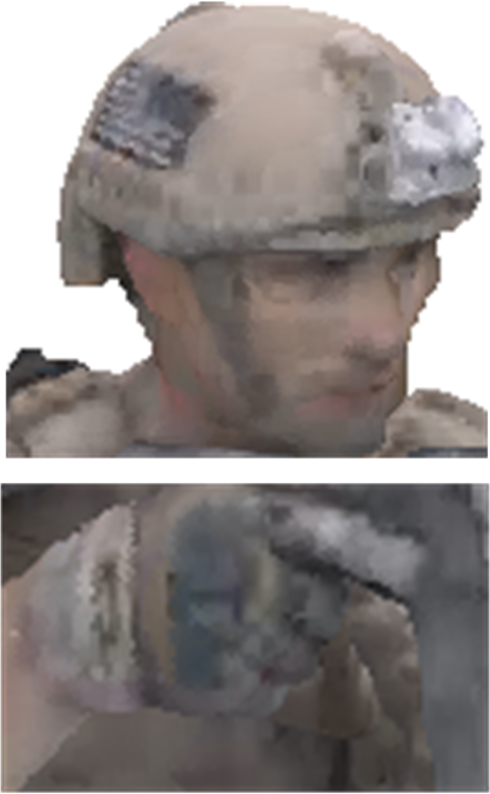
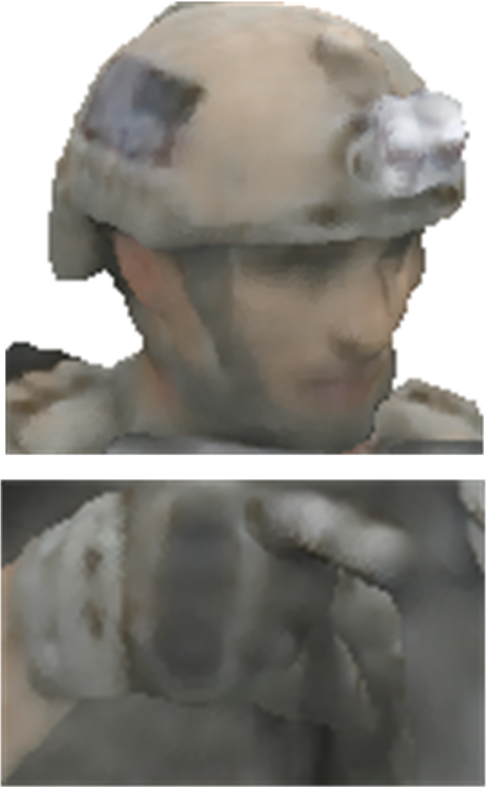
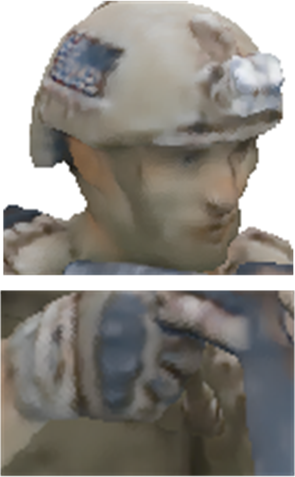
Figure 7: Visual quality comparison of the compressed point clouds. Digitalis in blanks denote the bit rate and quality, i.e. (bpp, PSNR). (a) Redandblack, (b) Enlarged Redandblack, (c) G-PCC v23 (0.102, 33.10dB), (d) Sparse-PCAC (0.143, 31.75dB), (e) NF-PCAC (0.116, 32.21dB), (f) TSC-PCAC (0.132, 33.24dB), (g) Soldier, (h) Enlarged Soldier, (i) G-PCC v23 (0.075, 30.42dB), (j) Sparse-PCAC (0.100, 29.75dB), (k) NF-PCAC (0.083, 29.87dB), (l) TSC-PCAC (0.084, 31.23dB).

IV-B Coding Efficiency Evaluation

Fig. 6 illustrates the coding results of Deep-PCAC, Sparse-PCAC, G-PCC, NF-PCAC and TSC-PCAC, where the vertical-axis is PSNR and the horizontal-axis is bit rate in terms of $bpp$. It can be observed that the Deep-PCAC performs the worst among all the methods. Sparse-PCAC, on the other hand, significantly outperforms the Deep-PCAC, but in the majority of point clouds, it is worse than the G-PCC. NF-PCAC has higher compression efficiency than Sparse-PCAC. As for the proposed TSC-PCAC, it outperforms the NF-PCAC by a large margin in all point clouds. Additionally, there are still a small number of point clouds where our method lags behind G-PCC such as Thaidancer. It is worth noting that TSC-PCAC shows a great improvement in the point clouds marked with * compared to G-PCC. This suggests that the network is capable of online learning from the first few frames to enhance compression efficiency for subsequent frames.

Table I presents the BD-BR and BD-PSNR value of TSC-PCAC compared to Sparse-PCAC, NF-PCAC and G-PCC on all testing point clouds. ‘Average’ is the average value over 9 point clouds, while the ‘Average*’ is the average result that includes point clouds marked with *. It can be observed that, without considering the point clouds marked with *, the proposed TSC-PCAC achieves bit-rate savings ranging from 30.12% to 50.14% compared to the Sparse-PCAC, with bit-rate savings of 36.62% on average. In terms of BD-PSNR, our method demonstrates improvements in reconstruction quality ranging from 1.17 dB to 2.35 dB across various point clouds, with 1.66 dB improvement on average, which is significant. As we include the seven point clouds marked with ‘*’ whose preorder frames were used in training and subsequent frames were used in testing, the proposed TSC-PCAC achieves bit rate savings ranging from 30.87% to 54.00% and 38.53% on average across various point clouds as compared with the Sparse-PCAC, which is more significant than the average value from point clouds without ‘*’. Moreover, the proposed TSC-PCAC achieves an average of 1.72 dB BD-PSNR gain. Compared to NF-PCAC, TSC-PCAC achieves bitrate savings ranging from 12.85% to 29.61%, with an average savings of 22.27%. In terms of BD-PSNR, our method shows improvements ranging from 0.47 dB to 1.25 dB, with an average improvement of 0.85 dB. When including point clouds marked with ‘*’, it achieves an average bitrate savings of 21.30% and a BD-PSNR gain of 0.80 dB, proving its superiority over NF-PCAC.

As compared to the G-PCC v23, the proposed TSC-PCAC achieves bitrate savings ranging up to 9.30% across different point clouds. However, for the Thaidancer point clouds, as shown in Fig. 6 and Table I, the proposed TSC-PCAC increases the bit rate by 28.01% compared with the G-PCC v23. The proposed TSC-PCAC is inferior to the G-PCC for Thaidancer mainly because the geometry and color of Thaidancer are relatively complex, and its PSNR value remains at a lower level even at higher bit rates. The different properties as compared with the training point clouds may degrade the performance of the learned codec. The TSC-PCAC is inferior to G-PCC v23 with an average of 1.26% bit rate increase and an average of 0.11 dB BD-PSNR degradation. However, as we include the seven point clouds marked with ‘*’, the proposed TSC-PCAC achieves an average of 11.19% bit rate saving and 0.34 dB BD-PSNR gain, which proves the effectiveness of the proposed TSC-PCAC. It indicates that the similarity between training and testing enables a better coding performance. Meanwhile, TSC-PCAC achieves coding gains for most point clouds.

IV-C Visual Quality Evaluation

In addition, visual quality comparisons were performed to validate the effectiveness of TSC-PCAC. Fig. 7 illustrates the visual quality with five different encoding methods across three test sequences. Figs. 7 to 7 display the enlarged detail images reconstructed by each encoding method for Redandblack. Figs. 7 to 7 correspond to Soldier. The red framed area in the image represents the visual focus on the face, while the green framed area depicts the clothing area with drastic color changes. To ensure fair comparisons, examples with similar bpp were selected. In the enlarged view of the face in Redandblack, more blocking artifacts are observed in the point cloud reconstructed from G-PCC v23 in Fig. 7. The bpp and PSNR are 0.102 and 33.10 dB. It exhibits noticeable block artifacts when compared to the original. In contrast, the point clouds reconstructed by the learning-based Sparse-PCAC shown in Fig. 7 and NF-PCAC shown in Fig. 7 have corresponding bpp and PSNR of 0.143 and 31.75 dB, and 0.116 and 32.21 dB, respectively, which appear smoother with a lower PSNR. The reconstructed point cloud of our TSC-PCAC is presented in Fig. 7 with bpp and PSNR of 0.132 and 33.24 dB. Compared to Sparse-PCAC and NF-PCAC, it exhibits a lower bit rate and higher PSNR. Additionally, in terms of visual quality, it can be observed that TSC-PCAC is smoother and offers better visual quality. Similar results can be found for Soldier from Figs. 7 to Fig. 7. In conclusion, compared to other encoding methods, the proposed TSC-PCAC achieves better reconstruction results under similar bitrate conditions or requires fewer bits for similar reconstruction results, demonstrating its effectiveness.

TABLE II: Coding and decoding complexity comparison among the TSC-PCAC, G-PCC, Sparse-PCAC, NF-PCAC and Deep-PCAC. [Uint:s].

PC	Deep-PCAC		Sparse-PCAC		GPCC v23		NF-PCAC		TSC-PCAC
	Enc. time	Dec. time	Enc. time	Dec. time	Enc. time	Dec. time	Enc. time	Dec. time	Enc. time	Dec. time
Soldier	28.26	23.77	66.78	294.57	5.53	4.95	1.99	2.45	1.62	4.49
Redandblack	17.89	14.88	43.44	151.94	3.70	3.31	1.37	1.67	1.41	3.39
Dancer	80.02	69.67	156.90	1135.91	13.40	12.08	4.45	5.48	2.85	9.79
Basketball Player	91.21	79.68	173.35	1364.30	14.82	13.37	4.85	5.98	3.14	10.66
Phil	40.33	33.99	70.66	323.55	7.38	6.62	2.53	3.09	1.87	5.54
Boxer	25.41	21.30	60.92	247.24	5.04	4.51	1.74	2.15	1.46	3.77
Thaidancer	16.24	13.42	37.86	122.97	3.34	2.99	1.45	1.76	1.30	3.22
Rafa	21.84	18.44	48.19	166.93	4.30	3.84	1.63	1.99	1.55	4.01
Sir Frederick	24.58	20.74	53.60	197.20	4.76	4.25	1.61	2.01	1.50	3.87
Andrew*	34.54	29.51	58.95	239.06	6.53	5.85	2.33	2.77	1.65	4.40
David*	54.83	46.92	93.58	473.10	9.52	8.55	3.19	3.86	2.22	7.41
Exerciese*	75.59	65.15	148.08	1062.44	12.80	11.52	3.60	4.69	2.44	7.85
Longdress*	20.03	16.60	48.87	178.55	4.10	3.67	1.60	1.94	1.54	4.17
Loot*	19.91	16.60	47.90	169.38	4.03	3.62	1.46	1.80	1.34	3.12
Model*	71.52	62.81	141.21	958.28	12.40	11.16	4.05	5.11	2.90	9.87
Sarah*	36.40	30.94	63.85	268.69	6.74	6.07	1.97	2.46	1.59	4.13
Average*	41.16	35.28	82.13	459.63	7.40	6.65	2.49	3.08	1.90	5.61

TABLE III: Computational complexity comparison

Methods	Sparse-PCAC	NF-PCAC	TSC-PCAC
Parameter	15.88M	51.16M	23.62M
Memory	4.75G	16.69G	5.58G
Y Enc.	0.11s	1.10s	0.20s
Y Entropy Enc.	82.02s	1.39s	1.70s
Total Enc.	82.13s	2.49s	1.90s
Y Entropy Dec.	459.29s	1.13s	5.16s
Y Dec.	0.34s	1.95s	0.45s
Total Dec.	459.63s	3.08s	5.61s

IV-D Computational Complexity Evaluation

We also evaluated the encoding and decoding time complexity of different codecs on all the testing point clouds. We processed each point cloud sequentially using a single GPU and the operating system was Ubuntu 22.04. For G-PCC, the encoding and decoding time for each point cloud corresponds to the average time required to encode and decode the point clouds using different QP settings. For the learned methods, the encoding and decoding time for each point cloud corresponds to the average time required to encode and decode the point clouds using networks with different $\lambda_{A}$ values.

From Table II, it can be observed that Deep-PCAC and Sparse-PCAC have relatively long encoding/decoding time, which are 41.16s/35.28s and 82.13s/459.63s, respectively. The longer encoding and decoding time for Deep-PCAC is due to the use of time-consuming operations such as the furthest point sampling in the network. For Sparse-PCAC, the long encoding and decoding time are caused by the sequential processing of the voxel context module. This issue becomes particularly severe when processing point clouds with more points and a precision of 11-bit, such as Basketball Player and Dancer, where the decoding time can exceed a thousand seconds. In contrast, G-PCC, NF-PCAC and TSC-PCAC are within the same level. For NF-PCAC, the average encoding/decoding time is 2.49s/3.08s. For G-PCC v23, the encoding/decoding time ranges from 3.44s/2.99s to 12.80s/11.52s, with an average of 7.40s/6.65s. The encoding/decoding time of TSC-PCAC ranges from 1.30s/3.22s to 3.14s/10.66s, with an average of 1.90s/5.61s. On average, TSC-PCAC reduces encoding/decoding time complexity by 97.68%/98.78%, 23.74%/-82.22% and 74.33%/15.66% compared to Sparse-PCAC, NF-PCAC and G-PCC v23. Note that the encoding and decoding of G-PCC were performed on CPU, while TSC-PCAC were performed on the GPU+CPU platform.

We also conducted a detailed analysis of the encoding and decoding time for learned compression methods. Table III illustrates the network parameters, memory consumption during testing, and the impact of each module on the encoding and decoding time. In the table, ‘Y Enc.’ represents the time required to obtain the latent representation ${\mathbf{y}}_{A}$ by the encoder, while ‘Y Dec.’ represents the time required to reconstruct the point cloud from the quantized latent representation $\mathbf{\hat{y}}_{A}$ by the decoder. Firstly, the parameter counts for sparse-PCAC, TSC-PCAC, and NF-PCAC are 15.88M, 23.62M, and 15.88M respectively. NF-PCAC has the largest number of network parameters, while Sparse-PCAC has the smallest, with our TSC-PCAC falling in between. Secondly, the encoder and decoder runtime for Sparse-PCAC is the shortest, while NF-PCAC takes the longest. However, Sparse-PCAC and TSC-PCAC use context modules, resulting in longer entropy encoding and decoding times compared to NF-PCAC. Sparse-PCAC employs the voxel context module, performing autoregression in spatial dimensions, while our TSC-PCAC utilizes the channel context module, performing autoregression in channel dimensions. Thus, our TSC-PCAC significantly reduces the number of autoregression steps required. This results in longer entropy encoding/decoding times for Sparse-PCAC, moderate times for TSC-PCAC, and the shortest times for NF-PCAC, which are 82.02s/459.29s, 1.70s/5.16s, and 1.39s/1.13s, respectively. Finally, the sum of the time required for encoder and entropy encoding yields the final encoding time, with TSC-PCAC being the shortest at an average of 1.90s. Similarly, the sum of the time required for decoder and entropy decoding yields the final decoding time, with NF-PCAC being the shortest at an average of 3.08s.

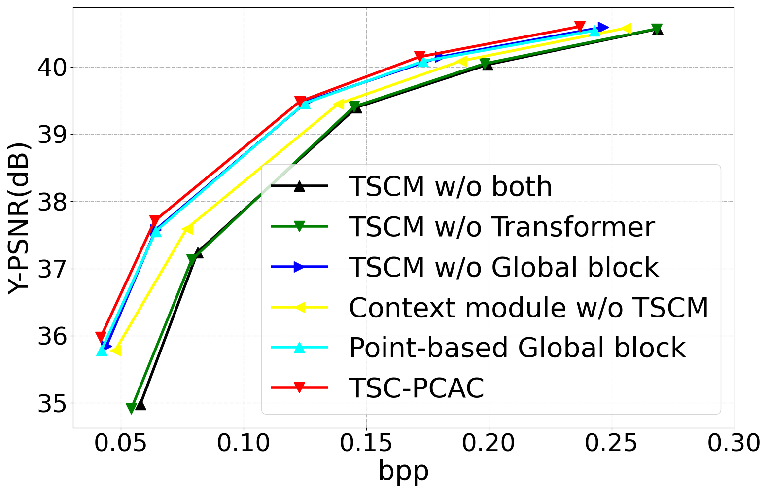
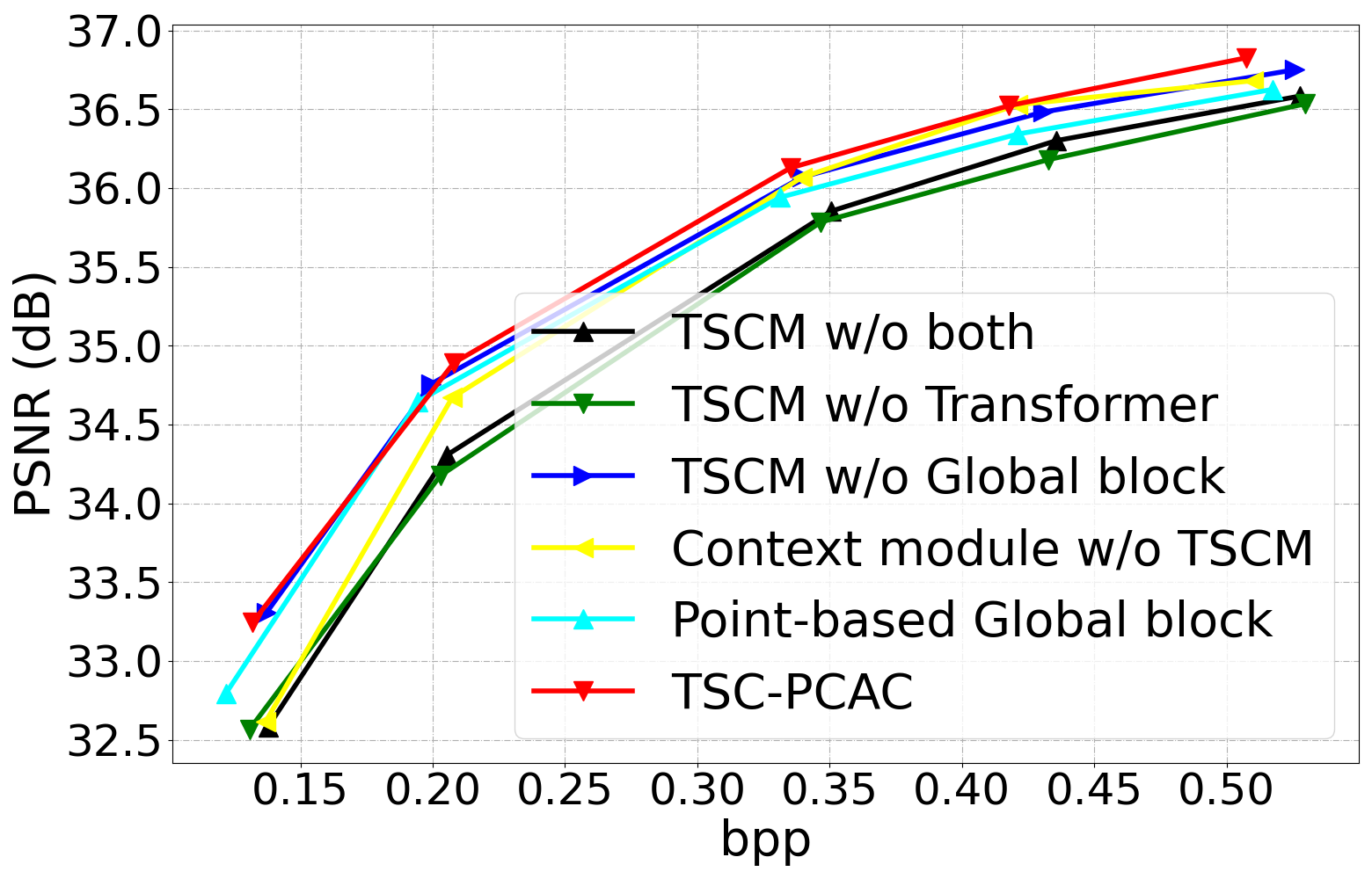
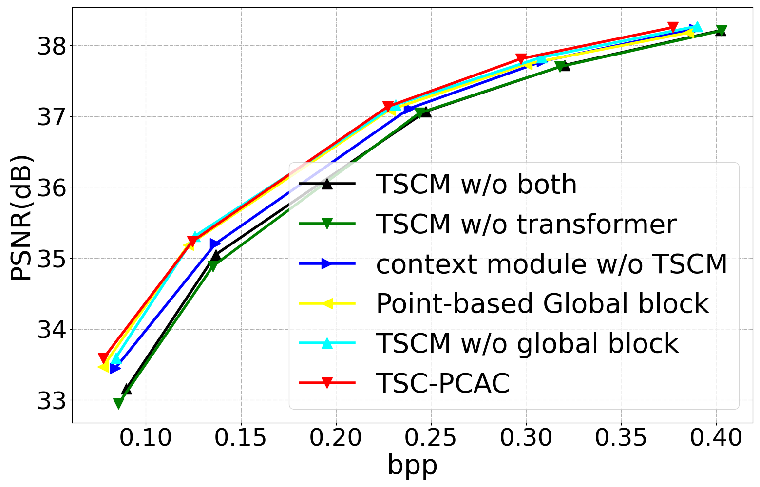
Figure 8: Average coding performance comparison for the TSC-PCAC ablation experiments. (a) Basketball Player, (b) Redandblack, (c) Average*

IV-E Ablation Study for TSC-PCAC

Ablation experiments were performed to validate the effectiveness of the TSCM, the TSCM based channel context module, and the voxel-based global module in TSC-PCAC. The experimental setup of the ablation study mirrored that of the TSC-PCAC. ‘TSCM w/o transformer’ represents the transformer in TSCM is replaced with residual block, ‘TSCM w/o global block’ represents the global block in TSCM is replaced with residual block, and ‘TSCM w/o both’ represents the global block and transformer in TSCM are replaced with residual block. ‘context module w/o TSCM’ indicates replacing TSCM with two convolutional layers in the channel context module. ‘Point-based Global block’ signifies the use of the global block from [38] to compose TSCM.

Fig. 8 and Table IV show the bitrate savings and PSNR gains achieved by different feature extraction modules compared to the baseline Sparse-PCAC. Notably, a module composed solely of residual blocks and global blocks achieves an average of 27.47% bitrate saving and an average of 1.19 dB PSNR gain. A module composed solely of residual blocks, on the other hand, achieves an average bitrate saving of 28.38% and PSNR gain of 1.23 dB, suggesting that using the global block alone is ineffective and can even degrade performance. A module consisting of only residual blocks and the transformer achieves an average of 36.09% bitrate savings and 1.60 dB PSNR gain. Finally, the TSCM module composed of residual blocks, global blocks, and transformer achieves the best encoding efficiency with an average of 38.53% bitrate saving and 1.72 dB PSNR gain. These results prove the effectiveness of combining the generalization features, global channel spatial features and local attention features.

TABLE IV: Coding Performance Ablation Study for the TSC-PCAC.

Methods	Methods vs Sparse-PCAC
	BD-BR-Y(%)	BD-PSNR-Y(dB)
Context w/o TSCM	-32.16	1.41
TSCM w/o Transformer	-27.47	1.19
TSCM w/o both	-28.38	1.23
TSCM w/o Global block	-36.09	1.60
Point-based Global block	-36.89	1.62
TSC-PCAC	-38.53	1.72

In addition, to evaluate the impact of the TSCM based channel context module, we replaced TSCM in the channel context with two convolutional layers as a benchmark, denoted as ‘context module w/o TSCM’. The channel context module consisting only of convolution has larger parameters than the channel context module with TSCM. Fig. 8 shows that the network using TSCM based channel context outperforms that of ‘context module w/o TSCM’ on various point clouds. Table IV illustrates that removing TSCM from the channel context saves only 32.16% bitrate on average compared to the baseline, which is inferior to the TSC-PCAC saving 38.53%. It demonstrates the effectiveness of incorporating the TSCM in the context module.

Lastly, we conducted an ablation experiment on the improved voxel-based global block compared to the original point-based global block. By using the original point-based global block, the TSC-PCAC is able to achieve an average of 36.89% bit rate reduction and an average of 1.62 dB BD-PSNR gain as compared with the Sparse-PCAC, which are inferior to the full TSC-PCAC using the proposed voxel-based global block. The results indicate that the voxel-based global block is more effective in the attribute coding.

V Conclusions

In this paper, we propose a voxel Transformer and Sparse Convolution-based Point Cloud Attribute Compression (TSC-PCAC) framework for point cloud broadcasting, in which an efficient Transformer and Sparse Convolution Module (TSCM) and TSCM based channel context module are developed to improve the attribute coding efficiency. The proposed TSCM integrates local dependencies and global spatial-channel features for point clouds, enabling modeling local correlations among voxels and capturing global features to effectively reduce redundancy. Furthermore, the TSCM based channel context module exploits inter-channel correlations to improve the predicted probability distribution of quantized latent representations, thereby reducing the bitrate. THe TSC-PCAC significantly outperforms the Sparse-PCAC, Deep-PCAC, NF-PCAC and G-PCC v23. Meanwhile, it performs with lower encoding/decoding complexity and better visualization than G-PCC. Overall, the TSC-PCAC is effective for point cloud attribute coding.

References

- [1] K. Mammou, P. A. Chou, D. Flynn, M. Krivokuća, O. Nakagami, and T. Sugio, G-PCC codec description v2, document ISO/IEC JTC1/SC29/WG11 N18189, 2019.
- [2] K. Mammou, A. M. Tourapis, D. Singer, and Y. Su, Video-based and hierarchical approaches point cloud compression, document ISO/IEC JTC1/SC29/WG11 m41649, Macau, China, 2017.
- [3] J. Liu, H. Sun, and J. Katto, “Learned image compression with mixed transformer-cnn architectures,” in Proc. IEEE Conf. Comput. Vis. Pattern Recog. (CVPR), 2023, pp. 14 388–14 397.
- [4] T. Huang and Y. Liu, “3d point cloud geometry compression on deep learning,” in Proc. ACM Int. Conf. Multimedia, 2019, pp. 890–898.
- [5] L. Gao, T. Fan, J. Wan, Y. Xu, J. Sun, and Z. Ma, “Point cloud geometry compression via neural graph sampling,” in Proc. IEEE Int. Conf. Image Process. (ICIP), 2021, pp. 3373–3377.
- [6] J. Wang, D. Ding, Z. Li, and Z. Ma, “Multiscale point cloud geometry compression,” in Proc. Data Compress. Conf. (DCC), 2021, pp. 73–82.
- [7] G. Liu, J. Wang, D. Ding, and Z. Ma, “Pcgformer: Lossy point cloud geometry compression via local self-attention,” in Proc. IEEE Int. Conf. Visual Commun. Image Process. (VCIP), 2022, pp. 1–5.
- [8] J. Wang, H. Zhu, H. Liu, and Z. Ma, “Lossy point cloud geometry compression via end-to-end learning,” IEEE Trans. Circuits Syst. Video Technol., vol. 31, no. 12, pp. 4909–4923, 2021.
- [9] J. Wang, D. Ding, and Z. Ma, “Lossless point cloud attribute compression using cross-scale, cross-group, and cross-color prediction,” in Proc. Data Compress. Conf. (DCC), 2023, pp. 228–237.
- [10] D. T. Nguyen and A. Kaup, “Lossless point cloud geometry and attribute compression using a learned conditional probability model,” IEEE Trans. Circuits Syst. Video Technol., vol. 33, no. 8, pp. 4337–4348, 2023.
- [11] X. Sheng, L. Li, D. Liu, Z. Xiong, Z. Li, and F. Wu, “Deep-pcac: An end-to-end deep lossy compression framework for point cloud attributes,” IEEE Trans. Multimedia, vol. 24, pp. 2617–2632, 2021.
- [12] J. Wang and Z. Ma, “Sparse tensor-based point cloud attribute compression,” in Proc. IEEE Int. Conf. Multimed. Inf. Process. Retr. (MIPR), 2022, pp. 59–64.
- [13] G. Fang, Q. Hu, H. Wang, Y. Xu, and Y. Guo, “3dac: Learning attribute compression for point clouds,” in Proc. IEEE Conf. Comput. Vis. Pattern Recog. (CVPR), 2022, pp. 14 799–14 808.
- [14] R. B. Pinheiro, J.-E. Marvie, G. Valenzise, and F. Dufaux, “Nf-pcac: Normalizing flow based point cloud attribute compression,” in Proc. IEEE Int. Conf. Acoust., Speech Signal Process. (ICASSP), 2023, pp. 1–5.
- [15] R. L. De Queiroz and P. A. Chou, “Compression of 3d point clouds using a region-adaptive hierarchical transform,” IEEE Trans. Image Process., vol. 25, no. 8, pp. 3947–3956, 2016.
- [16] C. Cao, M. Preda, V. Zakharchenko, E. S. Jang, and T. Zaharia, “Compression of sparse and dense dynamic point clouds—methods and standards,” Proc. IEEE, vol. 109, no. 9, pp. 1537–1558, 2021.
- [17] D. Graziosi, O. Nakagami, S. Kuma, A. Zaghetto, T. Suzuki, and A. Tabatabai, “An overview of ongoing point cloud compression standardization activities: Video-based (v-pcc) and geometry-based (g-pcc),” APSIPA Trans. Signal Inf. Proc., vol. 9, p. e13, 2020.
- [18] M. Yang, Z. Luo, M. Hu, M. Chen, and D. Wu, “A comparative measurement study of point cloud-based volumetric video codecs,” IEEE Trans. Broadcast., vol. 69, no. 3, pp. 715–726, 2023.
- [19] E. Pavez, A. L. Souto, R. L. De Queiroz, and A. Ortega, “Multi-resolution intra-predictive coding of 3d point cloud attributes,” in Proc. IEEE Int. Conf. Image Process. (ICIP), 2021, pp. 3393–3397.
- [20] P. Gao, L. Zhang, L. Lei, and W. Xiang, “Point cloud compression based on joint optimization of graph transform and entropy coding for efficient data broadcasting,” IEEE Trans. Broadcast., vol. 69, no. 3, pp. 727–739, 2023.
- [21] Y. Zhang, K. Ding, N. Li, H. Wang, X. Huang, and C.-C. J. Kuo, “Perceptually weighted rate distortion optimization for video-based point cloud compression,” IEEE Trans. Image Process., vol. 32, pp. 5933–5947, 2023.
- [22] X. Wu, Y. Zhang, C. Fan, J. Hou, and S. Kwong, “Subjective quality database and objective study of compressed point clouds with 6dof head-mounted display,” IEEE Trans. Circuits Syst. Video Technol., vol. 31, no. 12, pp. 4630–4644, 2021.
- [23] Q. Liang, Z. He, M. Yu, T. Luo, and H. Xu, “Mfe-net: A multi-layer feature extraction network for no-reference quality assessment of 3-d point clouds,” IEEE Trans. Broadcast., vol. 70, no. 1, pp. 265–277, 2024.
- [24] Y. Zhang, H. Liu, Y. Yang, X. Fan, S. Kwong, and C. C. J. Kuo, “Deep learning based just noticeable difference and perceptual quality prediction models for compressed video,” IEEE Trans. Circuits Syst. Video Technol., vol. 32, no. 3, pp. 1197–1212, 2022.
- [25] J. Xing, H. Yuan, R. Hamzaoui, H. Liu, and J. Hou, “Gqe-net: a graph-based quality enhancement network for point cloud color attribute,” IEEE Trans. Image Process., vol. 32, pp. 6303–6317, 2023.
- [26] J. Ballé, D. Minnen, S. Singh, S. J. Hwang, and N. Johnston, “Variational image compression with a scale hyperprior,” in Proc. Int. Conf. Learn. Represent., 2018, pp. 1–23.
- [27] Z. Tang, H. Wang, X. Yi, Y. Zhang, S. Kwong, and C.-C. J. Kuo, “Joint graph attention and asymmetric convolutional neural network for deep image compression,” IEEE Trans. Circuits Syst. Video Technol., vol. 33, no. 1, pp. 421–433, 2022.
- [28] R. Zou, C. Song, and Z. Zhang, “The devil is in the details: Window-based attention for image compression,” in Proc. IEEE Conf. Comput. Vis. Pattern Recog. (CVPR), 2022, pp. 17 492–17 501.
- [29] D. Minnen and S. Singh, “Channel-wise autoregressive entropy models for learned image compression,” in Proc. IEEE Int. Conf. Image Process. (ICIP), 2020, pp. 3339–3343.
- [30] D. Minnen, J. Ballé, and G. D. Toderici, “Joint autoregressive and hierarchical priors for learned image compression,” Proc. Adv. Neural Inf. Process. Syst., pp. 10 794–10 803, 2018.
- [31] R. Song, C. Fu, S. Liu, and G. Li, “Efficient hierarchical entropy model for learned point cloud compression,” in CVPR, 2023, pp. 14 368–14 377.
- [32] C. Szegedy, S. Ioffe, V. Vanhoucke, and A. Alemi, “Inception-v4, inception-resnet and the impact of residual connections on learning,” in Proc. AAAI Conf. Artif. Intell., no. 1, 2017, pp. 4278–4284.
- [33] A. Akhtar, Z. Li, and G. Van der Auwera, “Inter-frame compression for dynamic point cloud geometry coding,” IEEE Trans. Image Process., vol. 33, pp. 584–594, 2024.
- [34] J. Zhang, J. Wang, D. Ding, and Z. Ma, “Scalable point cloud attribute compression,” IEEE Trans. Multimedia, 2023.
- [35] C. R. Qi, L. Yi, H. Su, and L. J. Guibas, “Pointnet++: Deep hierarchical feature learning on point sets in a metric space,” Proc. Adv. Neural Inf. Process. Syst., pp. 5105–5114, 2017.
- [36] C. Choy, J. Gwak, and S. Savarese, “4d spatio-temporal convnets: Minkowski convolutional neural networks,” in Proc. IEEE Conf. Comput. Vis. Pattern Recog. (CVPR), 2019, pp. 3075–3084.
- [37] T. Zhao, N. Zhang, X. Ning, H. Wang, L. Yi, and Y. Wang, “Codedvtr: Codebook-based sparse voxel transformer with geometric guidance,” in Proc. IEEE Conf. Comput. Vis. Pattern Recog. (CVPR), 2022, pp. 1435–1444.
- [38] S. Qiu, S. Anwar, and N. Barnes, “Pnp-3d: A plug-and-play for 3d point clouds,” IEEE Trans. Pattern Anal. Mach. Intell., vol. 45, no. 1, pp. 1312–1319, 2021.
- [39] P. A. C. Sebastian Schwarz and I. Sinharoy, Common test conditions for point cloud compression, ISO/IEC JTC1/SC29/WG11 N18474, 2018.
- [40] D. Tian, H. Ochimizu, C. Feng, R. Cohen, and A. Vetro, Updates and Integration of Evaluation Metric Software for PCC, document ISO/IEC JTC1/SC29/WG11 MPEG2016/M40522, 2017.
- [41] G. Bjontegaard, Calculation of average PSNR differences between RD-curves, document VCEG-M33, 2001.
- [42] E. d’Eon, B. Harrison, T. Myers, and P. A. Chou, 8i Voxelized Full Bodies-a Voxelized Point Cloud Dataset, document ISO/IEC JTC1/SC29 Joint WG11/WG1 (MPEG/JPEG) WG11M40059/WG1M74006, 2017.
- [43] Y. Xu, Y. Lu, and Z. Wen, “Owlii Dynamic human mesh sequence dataset,” document ISO/IEC JTC1/SC29/WG11 M41658, 2017.
- [44] M. Krivokuca, P. A. Chou, and P. Savill, 8i Voxelized Surface Light Field (8iVSLF) Dataset, document ISO/IEC JTC1/SC29/WG11 MPEG, m42914, 2018.
- [45] R. Pagés, K. Amplianitis, J. Ondrej, E. Zerman, and A. Smolic, Volograms & V-SENSE Volumetric Video Dataset, document ISO/IEC JTC1/SC29/WG07 MPEG2021/m56767, 2021.
- [46] C. Loop, Q. Cai, S. O. Escolano, and P. A. Chou, Microsoft Voxelized Upper Bodies-a Voxelized Point Cloud Dataset, document ISO/IEC JTC1/SC29 Joint WG11/WG1 (MPEG/JPEG) m38673/M72012, 2016.
- [47] D. T. Nguyen, M. Quach, G. Valenzise, and P. Duhamel, “Lossless coding of point cloud geometry using a deep generative model,” IEEE Trans. Circuits Syst. Video Technol., vol. 31, no. 12, pp. 4617–4629, 2021.