LiDAR-based Real-Time Object Detection and Tracking in Dynamic Environments

Abstract

In dynamic environments, the ability to detect and track moving objects in real-time is crucial for autonomous robots to navigate safely and effectively. Traditional methods for dynamic object detection rely on high accuracy odometry and maps to detect and track moving objects. However, these methods are not suitable for long-term operation in dynamic environments where the surrounding environment is constantly changing. In order to solve this problem, we propose a novel system for detecting and tracking dynamic objects in real-time using only LiDAR data. By emphasizing the extraction of low-frequency components from LiDAR data as feature points for foreground objects, our method significantly reduces the time required for object clustering and movement analysis. Additionally, we have developed a tracking approach that employs intensity-based ego-motion estimation along with a sliding window technique to assess object movements. This enables the precise identification of moving objects and enhances the system’s resilience to odometry drift. Our experiments show that this system can detect and track dynamic objects in real-time with an average detection accuracy of 88.7% and a recall rate of 89.1%. Furthermore, our system demonstrates resilience against the prolonged drift typically associated with front-end only LiDAR odometry.

All of the source code, labeled dataset, and the annotation tool are available at: https://github.com/MISTLab/lidar_dynamic_objects_detection.git

I Introduction

Typically, when estimating the movement of robots, the assumption is that the surroundings are static[1, 2, 3]. However, this assumption is now being challenged more frequently in recent research. This is due to significant progress in the area of ego-motion estimation [4, 5, 6] and an increasing need for autonomous robots to work in dynamic environments[7, 8], such as urban areas, warehouses, and construction sites. In these settings, the presence of moving objects like pedestrians, cyclists, and other vehicles can greatly affect the robot’s ability to determine its location and map the area. Consequently, the robot’s capability to identify and track moving objects in real time becomes a crucial task.

Detecting and tracking moving objects in real time is a complex task. It demands that the robot can distinguish between static and moving objects, and track the motion of these moving objects in real time. This task is particularly challenging for robots that depend on Light Detection and Ranging (LiDAR) data for perception, as the data is typically unordered and noisy. In contrast to camera-based systems, which can obtain real-time semantic information of objects for tracking [9, 10, 11, 12, 13], processing LiDAR data is not as straightforward and efficient due to the higher dimensionality, increased number of points, and the sparse nature of point clouds compared to image data.

Figure 1: Illustration of dynamic object detection. Top: The raw intensity image. Middle: Dynamic objects are highlighted in red within the intensity image. Bottom: Dynamic points corresponding to these objects are extracted from the raw 3D point cloud, showing their spatial distribution.

At present, LiDAR-based techniques for identifying moving objects are categorized into two primary groups: map-based methods, and segmentation-based approaches[14, 15, 16], each coming with inherent limitations. Map-based methods demand extensive computational resources for map creation, making them unsuitable for real-time applications. Besides, those techniques struggle with complex environments and require increased computational effort as the size of the map grows. On the other hand, Segmentation-based approaches face challenges in accurately detecting objects within complex environments filled with unidentified objects, and their performance heavily depends on the objects’ visual characteristics.

To address these challenges, we propose a mapless dynamic object detection and tracking system. Our method first transforms the unordered point cloud data into an intensity image. This image then undergoes a process of 2D gaussian convolution to reduce its high-frequency components. This step helps in reducing noise and simplifying the distinction between foreground objects and the background. The 3D points that belong to the features of these foreground objects are retrieved from the original LiDAR data. By using intensity-based ego-motion estimation[17] , our system can track various object clusters in real-time. Analyzing the movement of these clusters, the system can identify the central points of moving objects within the environment and, through region growing, reconstruct the entire set of points that make up these moving objects[18, 19].

The main contributions of this work are summarized as follows:

1. Innovative Processing of LiDAR Data: We propose a novel method for processing LiDAR data by converting unordered point clouds into intensity images and applying 2D convolution. This technique effectively minimizes noise and accentuates the features of foreground objects, facilitating their identification and tracking. This represents a considerable advancement over conventional methods that struggle to process LiDAR data effectively;

2. Efficient Object Clustering and Identification: Employing intensity-based ego-motion estimation alongside a sliding window technique, our system excels in tracking clusters of objects in real time. Analyzing the movement of these clusters enables the identification of the central points of moving objects, leading to the accurate reconstruction of their full point sets. This method significantly enhances the system’s efficiency in recognizing and tracking objects within its surroundings;

3. Real-Time Detection and Tracking of Dynamic Objects: Our method encompasses a robust system for detecting and tracking dynamic objects in real time. Using LiDAR data, we distinguish between static and dynamic objects and track their movements with high precision. This capability is essential for navigating environments populated with frequently moving objects;

4. Robust Reconstruction of Dynamic Objects: Using intensity image based region growing techniques, our method reconstructs the complete set of points that make up moving objects. This enables the identification of the objects’ structures and positions within the environment, which is crucial for navigation and task execution. This robust reconstruction capability marks a significant improvement over prior techniques, which offer only partial or less precise representations.

This article is structured as follows: Section II offers a review of related work, focusing on the progress and challenges in the dynamic object detection. This sets the stage for our research by providing necessary background and justification. Section III elaborates on our proposed methodology. It details the process of converting LiDAR point clouds into intensity images, applying 2D convolution for background reduction, and tracking dynamic objects using intensity-based ego-motion estimation, clustering, estimation of movement combined with a sliding window approach. Section IV is dedicated to the experimental evaluation of our approach. It includes a comparative analysis with existing methods, demonstrating the effectiveness of our system in handling dynamic environments.

Section V summarizes the main contributions of our work and highlights its significance in enhancing robotic capabilities for navigating and operating in dynamic, complex environments. It also addresses the limitations of our study and proposes future research directions, suggesting advancements in ego-motion estimation and dynamic object tracking. We discuss the broader implications of our findings, the potential applications of our method, and how our work contributes to the field of robotics, particularly in terms of autonomous navigation.

II Related Work

II-A Map-based methods

Map-based methods for the detection of dynamic objects can be categorized into three primary types: ray-tracing methods, visibility-based methods, and occupancy-based methods.

Ray-Tracing Methods

Ray-tracing methodologies simulate LiDAR sensor behavior by tracing rays from the LiDAR sensor outward into the environment[20, 21]. Rays are traced through either the grid map [22] or voxel map [23] to identify dynamic objects. Should a ray traverse a grid cell or voxel, this indicates that the cell is empty. If an object obstructs the ray within this empty cell, it signifies that the object is dynamic.

Azim and Aycard [20] used an octree-based occupancy grid map to represent the dynamic surroundings of the vehicle and identified moving objects by noting discrepancies across scans. If the ray were reflected, then that volume would be occupied. If the ray were to traverse the volume, then it would be free. Peopleremover [21] efficiently removes dynamic objects from 3D point cloud data by constructing a regular voxel occupancy grid and traversing it along the sensor’s line of sight to the measured points to identify differences in voxel cells between different frames, which correspond to dynamic points. It is applicable to both mobile mapping and terrestrial scan data, aiming to produce a clean point cloud devoid of dynamic objects, such as pedestrians and vehicles. This process conservatively removes volumes only when they are confidently identified as dynamic, thus preserving the integrity of static elements in the point cloud data. Khronos [24] introduces a method for detecting dynamic objects in robotic vision systems using ray tracing. Instead of relying on volumetric data, it captures changes through surface representations and background and robot poses. By creating a library of rays between observed background vertices and robot positions, stored in a global hash map for efficiency, the method dynamically detects objects without real-time free-space mapping. Object detection is achieved by computing distances to rays, determining occlusion, consistency, or absence. This technique offers a practical approach to real-time object detection, balancing computational efficiency with accuracy. However, it perform poorly in dynamic environments with large open spaces with sparse surfaces. M-detector [18] is a motion event detection system inspired by the human visual system’s Magnocellular cells, known for their motion sensitivity due to larger sizes and faster processing capabilities. Using ray tracing and the principle of occlusion, it detects moving objects by observing how they interrupt the LiDAR sensor’s laser rays, effectively occluding previously visible backgrounds or recursively occluding themselves. The system processes inputs either as individual points or frames, applying three parallel occlusion tests to determine motion events. This approach allows for low-latency, high-accuracy detection without requiring extensive training datasets. M-detector’s design ensures it is highly generalizable, capable of detecting various object sizes, colors, and shapes across different environments with minimal computational resources, making it suitable for a wide range of robotic applications.

However, Ray-tracing methods demonstrate a significant sensitivity to the accuracy of odometry and incur substantial computational expenses during the construction of maps and and as the map size gradually increases [14, 25, 26, 27]. Additionally, these methods lead to increased computational times [24] with prolonged operation and prove unsuitable for real-time applications.

II-A1 Visibility-Based Methods

Visibility-based algorithms operate on a fundamental physical premise: light travels in straight lines, and if two points, one nearer and the other farther, are detected on the same ray, the nearer point has to be dynamic[26, 28, 29] to allow visibility of the farther point. The core concept involves recognizing dynamic points by examining the geometric variances between a query range image and its equivalent map range image. In essence, if a pixel’s range value in the query image surpasses the one in the map image, it indicates an occlusion at the map image pixel’s location according to these methods. Therefore, points mapped onto these pixels are deemed dynamic[25].

Removert [19] introduces a novel method for the removal of dynamic objects from LiDAR point cloud data. This method exploits the visibility of points within the LiDAR data to identify dynamic objects. By comparing the visibility of points in the current frame to that in the map, the method can detect dynamic objects and subsequently remove them from the point cloud data. This approach proves effective in removing dynamic objects from LiDAR data and enhancing the accuracy of static object detection. However, it is an offline method and is not suitable for real-time applications. ReFusion [30] creates a dense mapping that can effectively handle dynamic environmental elements without relying on specific dynamic object class detection, using Truncated Signed Distance Function (TSDF) and voxel hashing on GPU. The method detects dynamic objects by leveraging residuals from the registration process and the explicit representation of free space in the environment, achieving geometric filtering of dynamic elements. However, maintaining a dense TSDF mapping can be computationally expensive and memory-intensive.

The accuracy of the pose estimation is critical to the performance of the visibility-based methods since they need to retrieve the corresponding points in the map according to the odometry information. Moreover, false negatives, which include but are not limited to self-interference within point clouds and false positives caused by parallel point discrepancies, misjudged occluded points, and contact point errors, directly undermine the reliability of dynamic points extraction [14]. Additionally, the invisibility of static points, although less common than false negatives, poses a more challenging problem to solve. For instance, when dynamic obstacles continuously block part or all of the LiDAR’s rays of light, the LiDAR fails to detect the static objects behind these dynamic obstacles, leading to a scenario where the dynamic obstacle’s point cloud is never identified and filtered out [25].

II-A2 Occupancy-Based Methods

Occupancy-based methods employ statistical models to estimate the likelihood of space being occupied, facilitating robust mapping of environments with dynamic or uncertain elements.

Dynablox [16] is a real-time, map-based dynamic object detection system. It incrementally estimates high-confidence free-space areas and leverages enhanced the Truncated Signed Distance Field (TSDF) [31] method for volumetric mapping. This approach enables robust detection of dynamic objects without assumptions about their appearance or the structure of the environment. The method demonstrated an Intersection over Union (IoU) of 86% and processed data at 17 frames per second (FPS) on a laptop-grade CPU in real-world datasets, surpassing appearance-based classifiers and approximating the performance of certain offline methods. However, the study also acknowledges certain limitations, including challenges in detecting extremely thin and sparsely measured objects, such as shades, due to the voxel-based map representation. It also relies on prior odometry to place points into map spaces. ERASOR2[25] is an instance level dynamic object removal system that can effectively remove dynamic points from 3D point cloud maps. It uses Pseudo Occupancy Grid Map to represent whether the regions are temporally occupied or not by calculating the probability of those regions. It also employs instance segmentation [32] estimates to identify and exclude dynamic points at the instance level, ensuring that static points are preserved with minimal loss. This approach allows for the precise removal of dynamic objects from the map, enhancing the map’s utility for navigation and planning tasks.

Nevertheless, these methods still require maintaining a map of the environment, which is memory-intensive and computationally demanding, especially for long runs.

Figure 2: The framework of our dynamic object detection system, consisting of three main components: data preprocessing, object tracking, and dynamic object detection. The data preprocessing component converts unordered LiDAR point cloud data into intensity images and extracts low-frequency components to represent foreground objects. Object tracking involves ego-motion estimation, clustering, and cluster association. The ego-motion estimation component calculates the robot’s movement between frames using intensity-based front-end odometry, providing real-time movement data despite potential noise and drift. The dynamic object detection component leverages data association results to track objects and identify seed points of dynamic objects, followed by a region growing algorithm to reconstruct the complete point set of dynamic objects from these seed points. This system processes LiDAR data in real-time to detect dynamic objects in complex environments, using the low-frequency components to represent foreground objects and enable real-time tracking across multiple frames.

II-B Segmentation-Based Methods

Segmentation-based methods focus on identifying dynamic objects by semantically segmenting the point cloud and analyzing the movement of points or objects over time. These methods are particularly effective in detecting dynamic objects in complex environments with unidentified objects.

Thomas et al. [33] proposed a self-supervised learning method for dynamic object detection in LiDAR point clouds. They first projected each frame of point cloud into 2D grids. Then, they stacked the 2D frames into 3D according to the time sequence. Finally, they used a KPConv network [34] 3D back-end and a three levels U-Net [35] 2D front-end to predict the future time steps of spatiotemporal occupancy grid maps. Chen et al. [36] used the range image to represent the point cloud data and combined the current frame and residual images generated between current frame and the last few frames. After then, they used a range projection-based segmentation CNNs [37, 38, 39] to predict the moving objects.

As an upgrade to [33], Sun et al. [40] extended the SalsaNext [39] by adopting a dual-branch (a range image branch and a residual image branch) and dual-head (an image head and a point head) architecture to separately deal with spatial and temporal information. After then, they used a 3D sparse convolution to refine the prediction results. In this coarse-to-fine framework, the network can predict the moving objects more accurately and efficiently. Mersch et al. [41] combined a sequence of LiDAR point cloud into a voxelized spare 4D point cloud. Then, they feeded the combined 4D occupancy grid to a modified MinkUNet14 [42] to extract spatio-temporal features and predicted the confidence score for each point.

These methods are effective in detecting dynamic objects; however, they predominantly depend on a substantial volume of annotations for the dynamic objects in the training data, which may not always be accessible. Furthermore, segmentation-based methods incur significant computational costs and frequently yield unsatisfactory results in unfamiliar environments. Consequently, a need persists for a lightweight and label-free method for dynamic object detection in real-time.

In this work, to increase speed and reduce computational load, we primarily concentrate on the low-frequency components of LiDAR data, which are used to represent foreground objects. Given that the size of the low-frequency components is significantly smaller than that of the original LiDAR data, our approach enables real-time tracking of multiple objects across multiple frames.

III Methodology

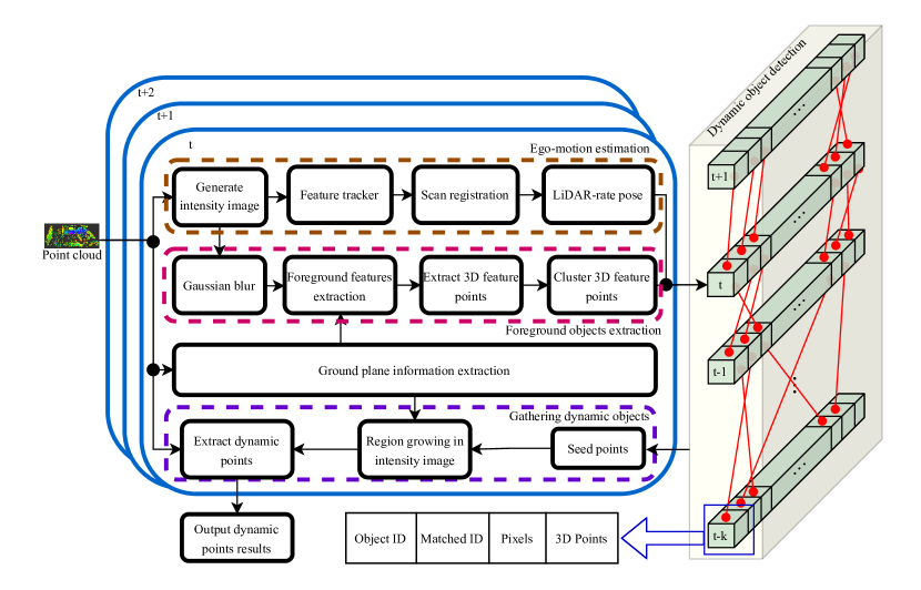
Our proposed method is illustrated in Fig 2. This framework principally comprises three components: data preprocessing, object tracking, and dynamic object detection. Our method is engineered to process

III-A Data Preprocessing

III-A1 Point Cloud to Intensity Image

Unlike cameras, which generate an image in each cycle, LiDARs produce a frame of point cloud data per cycle. Each point $\mathbf{p}$ within this frame records spatial dimensions and intensity information, $\mathbf{p}=\{x,y,z,i\}$. The intensity of a point is determined by the signal, which constitutes the number of photons collected by the sensor for a pixel during a single cycle. The initial step of our method involves converting the unordered LiDAR point cloud data into an intensity image through spherical projection. This process entails projecting the point cloud data onto a two-dimensional grid; each grid cell therein represents the intensity of the points contained within it. The grid cell’s index $(u,v)$ can be determined by the following equation:

$$\left[\begin{array}[]{c}u\\ v\end{array}\right]=\left[\begin{array}[]{c}\frac{\left(\arctan(y,x)+\pi\right)}{2\pi}\cdot w\\ \frac{\left(\beta_{up}-\arcsin(zr^{-1})\right)}{\beta_{fov}}\cdot h\end{array}\right]$$ (1)

Where the $r$ represents the distance between the point and the sensor, denoted as $||\mathbf{p}||_{2}$, $w$ and $h$ are the width and height of the image, respectively, and $\beta_{up}$ and $\beta_{fov}$ are the upper bound and field of view of the LiDAR sensor, respectively.

By converting the point cloud data into an intensity image, we treat the unordered LiDAR data similarly to an image, simplifying subsequent processing steps. This transformation permits the application of image processing techniques to LiDAR data, thus facilitating the identification and tracking of dynamic objects.

III-A2 Low-frequency components extraction

The intensity image generated in the previous step contains high-frequency components that can significantly slow down the clustering and tracking processes. In order to extract features of the foreground objects with fewer points, we apply a 2D gaussian convolution to the intensity image to extract low-frenquency components, see (3), and treat them as a representative of foreground objects. This process involves convolving the intensity image with a 2D Gaussian kernel which effectively smooths the image and minimizes noise:

$$g(m,n)=\frac{1}{2\pi\sigma_{m}\sigma_{n}}\exp\left(-\left(\frac{m^{2}}{2\sigma_{m}^{2}}+\frac{n^{2}}{2\sigma_{n}^{2}}\right)\right)$$ (2)

Here, $m$ and $n$ represent the distances from the center of the kernel to the current point and can take integer values, including negative ones. $m$ ranges from $[-a,a]$ and $n$ ranges from $[-b,b]$. In this case, as the intensity image is quite flat, we also configure the kernel to have a flat shape, where $a>b$. This configuration ensures that the Gaussian kernel matrix’s index for the center of columns is 0, with $a$ positions on either side, and similarly, the center index for rows is 0, with $b$ positions on each side. $\sigma_{m}$ and $\sigma_{n}$ denote the standard deviations along the horizontal and vertical directions, respectively. The Gaussian kernel size is $(2a+1,2b+1)$. Then, we convolve the intensity image with the Gaussian kernel to extract the low-frequency components:

$$h(u,v) =(f*g)(u,v)$$ (3)

$$=\sum_{m=-a}^{a}\sum_{n=-b}^{b}f(u-m,v-n)\cdot g(m,n)$$

where $f(u-m,v-n)$ represents the intensity value of the image at position $(u-m,v-n)$, and $g(m,n)$ represents the value of the kernel at position $(m,n)$. The variables $m$ and $n$ are the distances from the center of the kernel, ranging over the kernel dimensions. The convolution operation is performed by sliding the kernel over the image and calculating the sum of the products of the kernel values and the image values at each position.

Finally, we subtract the blurred image from the original intensity image, as shown in (4). The resulting image retains only the low-frequency components, which depict the features of the foreground objects. By focusing on these low-frequency components, we are able to accurately identify and track dynamic objects in real-time.

$$t(u,v)=B\left(f(u,v)-h(u,v),\theta\right)$$ (4)

where $B(x,\theta)$ is a binarization function defined by:

$$B(x,\theta)=\begin{cases}1&\text{if }x>\theta\\ 0&\text{otherwise}\end{cases}$$

and $\theta$ is the threshold value.

III-B Object Tracking

After extracting the low-frequency components from the intensity image, the 3D points associated with the features of these foreground objects can be further extracted from the raw LiDAR data. Subsequently, these points can be clustered into distinct objects and tracked in real-time, owing to their small number.

III-B1 Intensity-based Ego-Motion Estimation

The initial step in object tracking involves estimating the ego-motion of the robot. This is accomplished by extracting ORB features [43] from the intensity image and calculating the transformation matrix between consecutive frames. The resulting transformation matrix is used to estimate the robot’s movement between frames, an essential factor for accurate object tracking. This technique, known as intensity-based ego-motion estimation, was proposed in our previous work [17]. Here we only use the front-end of the SLAM system to make is lightweight and real-time, but drift may occur during long-term operation. However, in the following we show that drift will not affect the object tracking accuracy.

For each frame of intensity image, we extract ORB features and match them with the features in the previous frame. At the same time, we can extract the corresponding 3D points from current and previous frames and put them into $\mathcal{X}=\{\mathbf{X}_{1},\mathbf{X}_{2},\cdots,\mathbf{X}_{k}\}$ and $\mathcal{Y}=\{\mathbf{Y}_{1},\mathbf{Y}_{2},\cdots,\mathbf{Y}_{k}\}$, respectively. Then, the scan match problem can be formulated as a least square estimation problem:

$$\mathop{\arg\min}_{\mathbf{R,t}}\sum\limits_{n\in\mathcal{N}}\parallel\mathbf{Y}_{n}-(\mathbf{R}_{i}\mathbf{X}_{n}+\mathbf{t}_{i})\parallel_{2}$$ (5)

where $\mathcal{N}=[1,2,\cdots,k]$, $\mathbf{X}_{n}=\{x_{n},y_{n},z_{n}\}$, and $\mathbf{R}_{i}$ and $\mathbf{t}_{i}$ are the rotation matrix and translation vector at current frame time $i$ with respect to the previous frames, respectively. The solution of this optimization problem is the ego-motion of the robot between two frames. So, we need to accumulate $\mathbf{R}_{i}$ and $\mathbf{t}_{i}$ to get the robot’s pose in a reference coordinate system.

III-B2 Clustering

Since the number of objects varies across different frames, traditional clustering methods that require predefined cluster numbers, such as K-means, cannot be employed. Furthermore, the vertical disparity between two adjacent laser beams increases as the distance to the objects increases. Consequently, addressing this challenge demands the use of a more robust clustering method. We initially employ an Euclidean distance-based clustering method to segment all points into groups, which are subsequently clustered into distinct objects.

As mentioned above, we can get 3D points $\mathcal{Q}=\{\mathbf{p}_{0},\mathbf{p}_{1},\cdots,\mathbf{p}_{n}\}$ that represent the features of the foreground objects. For each point in $\mathcal{Q}$, we calculate the Euclidean distance between it and all other points in horizontal and vertical plane, see (6).

$$\mathbf{d}({\mathbf{p}_{i}},\mathbf{p}_{j})=\left[\begin{array}[]{c}d_{xy}(\mathbf{p}_{i},\mathbf{p}_{j})\\ d_{z}(\mathbf{p}_{i},\mathbf{p}_{j})\end{array}\right]=\left[\begin{array}[]{c}\sqrt{(x_{i}-x_{j})^{2}+(y_{i}-y_{j})^{2}}\\ |z_{i}-z_{j}|\end{array}\right]$$ (6)

The points $i$ and $j$ can be clustered into the same group $\mathcal{C}_{m}=\{\mathbf{p}_{i},\mathbf{p}_{j},\cdots,\mathbf{p}_{k}\}$ if the distance between them is less than a predefined threshold, $\epsilon$. The clustering process can be formulated as (7):

$$\forall\mathbf{p}_{i},\mathbf{p}_{j}\in\mathcal{C}_{m},\quad\mathbf{d}({\mathbf{p}_{i}},\mathbf{p}_{j})\leq\mathbf{\epsilon}$$ (7)

After clustering, we get a group of clusters $C=\{\mathcal{C}_{1},\mathcal{C}_{2},\cdots,\mathcal{C}_{m},\cdots,\mathcal{C}_{q}\}$, and the total number of cluster $q$ can be different for each frame.

III-B3 Cluster Association

The clusters need to be linked between frames to ensure the continuity of the tracking process. We use the Global Nearest Neighbor (GNN) [44] method for this association. We first calculate the center point of each cluster in the current frame, $\mathbf{c}_{m}^{i}=[x_{m},y_{m},z_{m}]^{T}$, and the center point of each cluster in the previous frame, $\mathbf{c}_{n}^{i-1}=[x_{n},y_{n},z_{n}]^{T}$. Then, we calculate the Euclidean distance between the center points of the clusters in the current frame and the previous frame:

$$d_{\mathbf{c}}(\mathbf{c}_{m}^{i},\mathbf{c}_{n}^{i-1})=\parallel\mathbf{c}_{m}^{i}-(\mathbf{R}_{i}\mathbf{c}_{n}^{i-1}+\mathbf{t}_{i})\parallel_{2}$$ (8)

Subsequently, we will build a cost matrix $\mathbf{D}\in\mathbb{R}^{M\times N}$, where $M$ and $N$ are the number of clusters in the current frame and the previous frame, respectively. Each element $d_{m,n}=d_{\mathbf{c}}(\mathbf{c}_{m}^{i},\mathbf{c}_{n}^{i-1})$ in the cost matrix represent the distance cost if the cluster $m$ in the current frame matches with the cluster $n$ in the previous frame. To filter out the unmatched clusters, distances exceeding the threshold $d_{max}$ are assigned a prohibitively high cost to prevent them from being selected in the optimization process:

$$d_{m,n}=\begin{cases}d_{\mathbf{c}}(\mathbf{c}_{m}^{i},\mathbf{c}_{n}^{i-1})&\text{if }d_{\mathbf{c}}(\mathbf{c}_{m}^{i},\mathbf{c}_{n}^{i-1})\leq d_{\text{max}}\\ \infty&\text{otherwise}\end{cases}$$ (9)

It is possible that some previously appearing objects do not appear in the current frame, while new objects might appear. To solve this problem, we add dummy targets to the cost matrix. The cost between dummy targets and real objects is set to a high value, which is $2d_{max}$ as penalty costs while the cost between dummy targets is set to 0. This way, the cost matrix can be extended to $\mathbf{D}\in\mathbb{R}^{(M+M^{\prime})\times(N+N^{\prime})}$. We can then use the Hungarian algorithm [45] to solve the assignment problem and get the optimal solution. The Hungarian algorithm is a combinatorial optimization algorithm that solves the assignment problem in polynomial time, ensuring that clusters are tracked across frames:

$$\min\sum_{m=1}^{M+M^{\prime}}\sum_{n=1}^{N+N^{\prime}}\alpha_{mn}d_{m,n}$$ (10)

where: $M^{\prime}$ and $N^{\prime}$ represent the number of dummy targets added to the current and previous frames respectively. Subject to the constraints:

$$\sum_{m=1}^{M+M^{\prime}}\alpha_{mn}=1\quad\text{for all }n\in\{1,\ldots,M+M^{\prime}\}$$ (11)

$$\sum_{n=1}^{N+N^{\prime}}\alpha_{mn}=1\quad\text{for all }m\in\{1,\ldots,N+N^{\prime}\}$$ (12)

$$\alpha_{mn}\in\{0,1\}$$ (13)

By employing this method, we guarantee that each cluster in the current frame is matched uniquely with a corresponding cluster from the previous frame, thus preserving the continuity of the tracking process.

III-C Dynamic Object Detection

III-C1 Movement Analysis

Following the process of cluster association, we can determine all matching clusters for all frames across a given time slot. To analyse the movement of the clusters in current frame, we first create a sliding window of a fixed size, $k$ from the initial to the current frame.

We accumulate the transformation matrix $\mathbf{T}_{i}$ between frame $i$ and the initial frame. From (5), we can get the relative rotation $\mathbf{R}_{i}$ and translation matrix $\mathbf{t}_{i}$ between current frame and previous frame. To simplify the following expression, we transform them from SO3 to SE3 and perform a homogeneous transformation on the cluster’s centroid.

$$\mathbf{T}=\left[\begin{array}[]{cc}\mathbf{R}&\mathbf{t}\\ \mathbf{0}^{T}&1\end{array}\right]=\left[\begin{array}[]{cccc}rx_{x}&ry_{x}&rz_{x}&x\\ rx_{y}&ry_{y}&rz_{y}&y\\ rx_{z}&ry_{z}&rz_{z}&z\\ 0&0&0&1\end{array}\right]$$ (14)

$$\mathbf{c}_{m}^{i}=[x_{m}^{i},y_{m}^{i},z_{m}^{i},1]^{T}$$ (15)

For frames inside the sliding window, we can get a series of transformation matrices $\mathbf{T}_{i}$, $i\in\{1,2,\cdots,k\}$. Then, we can calculate the relative transformation matrix between the frame $i$ and the initial frame:

$$\mathbf{T}_{i}^{w}=\prod_{j=1}^{i}\mathbf{T}_{j}$$ (16)

Where, $\mathbf{T}_{i}^{w}$ is the relative transformation matrix between the frame $i$ and the initial frame, and $\mathbf{T}_{j}$ is the transformation matrix between the frame $j$ and frame $j-1$.

Then, we can transform the cluster’s centroid in the current frame to the initial frame:

$$\mathbf{c}_{m}^{wi}=\mathbf{T}_{i}^{w}\mathbf{c}_{m}^{i}$$ (17)

Here, $\mathbf{c}_{m}^{wi}$ represents the centroid of cluster $m$ in the $i$th frame within the initial frame’s coordinate system. Having already transformed the centroid of the cluster from the current frame to the initial frame, we can now employ the format used prior to the homogeneous transformation. Consequently, the cluster’s centroid in the initial frame can be represented as:

$$\mathbf{c}_{m}^{wi}=[x_{m}^{wi},y_{m}^{wi},z_{m}^{wi}]^{T}$$ (18)

where $x_{m}^{wi}$, $y_{m}^{wi}$, and $z_{m}^{wi}$ represent the $x$, $y$, and $z$ coordinates of the centroid position of cluster $m$ of the $i$th frame in the initial frame’s coordinate system. inline]I think we are missing the description of some terms

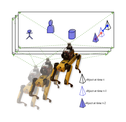
We can then track pairs of matched clusters to the initial frame if they exist. Figure 3 shows the object tracking principles. We can finally calculate the Euclidean distance between the cluster’s centroid in the current frame and the initial frame:

$$f(\mathbf{c}_{m}^{wk},\mathbf{c}_{m}^{w1})=\parallel\mathbf{c}_{m}^{wk}-\mathbf{c}_{m}^{w1}\parallel_{2}$$ (19)

if the distance is less than a predefined threshold, $\epsilon_{d}$, we can consider the cluster as a dynamic object.

Figure 3: Dynamic Object Tracking: to adapt to the drift of the front-end odometry, we accumulate the transformation matrix between the current frame and the first frame within a time window. This approach allows us to ignore historical drift and only account for the drift within the current time window. By transforming all frames into the same coordinate system, we can calculate the distance between the centroids of clusters in consecutive frames and match corresponding clusters between frames. This method enables real-time tracking of all detected foreground objects. By analyzing the movement of clusters within the sliding window, we can effectively detect dynamic objects. In the picture, three frames within the time window are transformed into the initial frame’s coordinate system. Although all clusters appear to move due to the odometry drift, the movement of static objects is minimal and usually follows a zero-mean Gaussian distribution. Therefore, we can filter out dynamic objects by accumulating the distance between the cluster’s centroid in the current frame and the initial frame.

III-C2 Outlier Detection

As we only rely on the front-end odometry, its drift may cause some outliers to appear as dynamic objects. To solve this problem, we can calculate the absolute distance of the matched clusters in the current frame:

$$f_{a}(\mathbf{c}_{m}^{wk},\mathbf{c}_{m}^{1})=\sum_{j=2}^{k}\parallel\mathbf{c}_{m}^{wj}-\mathbf{c}_{m}^{w(j-1)}\parallel_{2}$$ (20)

if the object is static and the drift noise follows a Gaussian distribution, $f(\mathbf{c}_{m}^{wk},\mathbf{c}_{m}^{w1})\approx 0$ and $f_{a}(\mathbf{c}_{m}^{wk},\mathbf{c}_{m}^{1})>0$. So, we can use the ratio of $f(\mathbf{c}_{m}^{wk},\mathbf{c}_{m}^{w1})$ and $f_{a}(\mathbf{c}_{m}^{wk},\mathbf{c}_{m}^{1})$ to filter out the outliers. If the ratio is less than a predefined threshold, $\epsilon_{o}$, we can consider the cluster as a dynamic object.

In addition to the drifting problem, we are also facing an issue with long objects being mistakenly identified as dynamic objects due to the sparse nature of LiDAR. As the robot moves forward and the LiDAR scans the surface of such objects, the shape of the cluster remains almost the same, causing the center of the object to appear to shift, creating the illusion of movement. Such clusters tend to grow as the robot moves forward, especially for objects that are long and parallel to the direction of movement. To solve this problem, we propose to calculate the cluster’s moving direction and the cluster’s main direction and compare the angle between them. If the angle is less than a predefined threshold, $\epsilon_{\theta}$, we can consider the cluster as a dynamic object. For a cluster $m$ in the current frame, we can calculate the moving direction as:

$$\vec{v}=\frac{\mathbf{c}_{m}^{wk}-\mathbf{c}_{m}^{w1}}{\parallel\mathbf{c}_{m}^{wk}-\mathbf{c}_{m}^{w1}\parallel_{2}}.$$ (21)

For the cluster $\mathcal{C}_{m}$, we can use Principal Component Analysis (PCA) to calculate its main direction $\mathbf{V}$:

$$\mathbf{V}=\text{PCA}(\mathcal{C}_{m}).$$ (22)

The angle between the moving direction and the main direction is then

$$\theta=\arccos(\vec{v}\cdot\mathbf{V}).$$ (23)

If $\theta$ is smaller than a predefined threshold, $\epsilon_{\theta}$, we can consider the cluster as an outlier.

III-C3 Region Growing

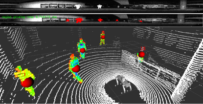
After removing the outliers, we have seed points for the dynamic objects in the current frame. After converting the seeds points from the initial coordinate frame to the current, we can get the dynamic objects’ center points’s pixel position in the raw intensity image (see Figure 1, top). A region growing method can be sued on the seed points to segment the whole dynamic object. The basic idea is to start from the seed points and grow the region by adding the neighboring points that have similar properties to the seed points. We use the Euclidean distance between the points to determine whether they are similar. However, finding the neighboring points in the raw point cloud is time-consuming. To solve this problem, we can use the intensity image to find the neighboring points. For each point in the intensity image, we can extract the surrounding pixels directly as neighboring points instead of comparing their Euclidean distance in the raw point cloud. The neighbor points of each seed points’ pixel index can be extracted as:

$$N_{8}(x,y)=\{(x+i,y+j)\mid i,j\in\{-1,0,1\},(i,j)\neq(0,0)\}$$ (24)

Where, $N_{8}(x,y)$ is the 8-neighborhood of the seeds point’s pixel $(x,y)$ in the intensity image.

The region growing process can be formulated as

$$\mathcal{Q}_{\text{new}}=\mathcal{Q}\cup\left\{\mathbf{p}_{j}\mid j\in N_{8}(i_{x},i_{y}),\exists\mathbf{p}_{i}\in\mathcal{Q},\quad\parallel\mathbf{p}_{i},\mathbf{p}_{j}\parallel_{2}\leq\mathbf{\epsilon}\right\}$$ (25)

where, $\mathcal{Q}$ is the set of seed points of the dynamic object, and $\mathbf{p}_{j}$ is a neighboring point of the seed points. If the distance between the neighboring points and a seed point is less than a predefined threshold, $\epsilon$, we can add the neighboring points to the dynamic object. This process is repeated until all eligible neighboring points are added to the dynamic object.

To prevent regions from absorbing all points we use the ground plane information to filter out neighboring points that do not belong to the dynamic object. Figure 1, middle, shows the dynamic object after the region growing process in red. Figure 1, bottom, shows the dynamic object points retrieved from the raw point cloud according to the dynamic object’s pixel index in the intensity image.

Figure 4: Spot robot navigating a dynamic environment. Equipped with an OS0-64 LiDAR sensor, the Spot robot moves through a large area filled with pedestrians as moving objects. Both the pedestrians and the Spot robot exhibit random movements, creating a constantly changing environment that challenges the robot’s navigation and object detection capabilities.

IV Experimental Evaluation

IV-A Dataset

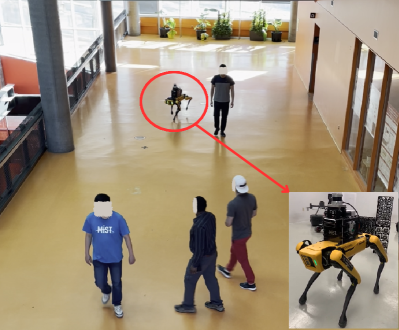
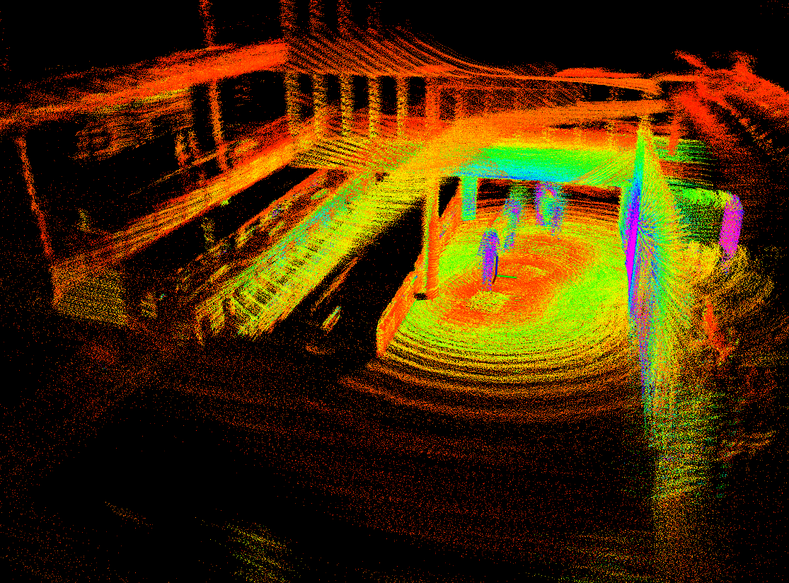
We used a Boston Dynamic Spot robot equipped with an Ouster 64-line LiDAR sensor to collect the dataset. The robot was driven around the floor of a large space with moving objects, shown in Figure 4. In normal conditions, the map is blurred by the movement of the pedestrians (Figure 5), and the moving objects affect the localization accuracy. We manually labeled the dynamic objects in the dataset to evaluate the performance of the proposed method. The labeled information was stored in the following format: {timestamp, dynamic points index}. The timestamp represents the time when the dynamic objects were detected, and the dynamic points index represents the pixel index of the dynamic objects in the intensity image.

To efficiently label streaming 3D dynamic points, we developed a specialized tool that allows users to label dynamic objects within an intensity image in a streaming style and store the labeled information in binary format.

When labeling dynamic objects, users can check previous and following frames to identify which points are dynamic. Users can then click the center of the dynamic object in the intensity image and apply a region growing method to capture all points belonging to the dynamic object. To aid in this process, the tool provides visual assistance by displaying the extracted foreground points in the intensity image, along with ground information. The labeling tool will be open-sourced

Figure 5: Point cloud map of the environment with dynamic objects. The dynamic points create blurring in the map as they move, highlighting the challenges of accurately mapping in dynamic environments.

IV-B Evaluation Metrics

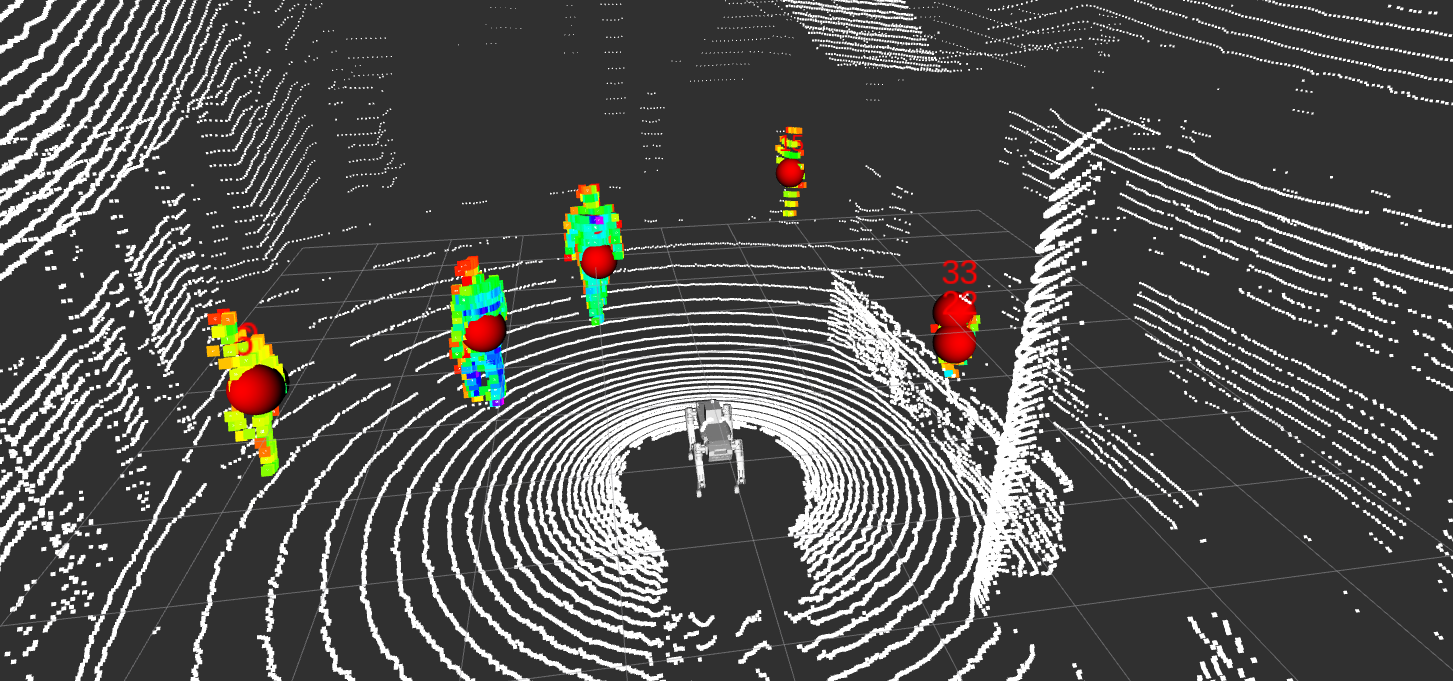
Due to the time consuming nature of labelling, we only labeled four sequences of the data collected from the Spot robot to assess the performance of the proposed method. The estimated dynamic objects are recorded in the same format as the labeled data. The performance of the proposed method is evaluated by comparing the labeled data with the ground truth provided by labeling. The estimated dynamic objects are showing in figure 6 with colorful points.

Figure 6: Segmentation results of dynamic objects in a single frame. The dynamic objects are segmented from the raw point cloud and displayed with colorful points. The center points of the dynamic objects are marked in red.

We used the following metrics to evaluate the performance of the proposed method: precision, recall, IoU, and F1 score[18, 25, 46]. These metrics are commonly used in object detection and tracking tasks and provide a comprehensive evaluation of the method’s performance:

• Precision: The ratio of correctly identified positive instances to the total instances identified as positive.

  $$\text{Precision}=\frac{TP}{TP+FP}$$ (26)

• Recall: The ratio of correctly identified positive instances to the total actual positive instances.

  $$\text{Recall}=\frac{TP}{TP+FN}$$ (27)

• IoU: The ratio of the overlap between the predicted and ground truth bounding boxes to the union of these boxes.

  $$\text{IoU}=\frac{\text{Area of Overlap}}{\text{Area of Union}}=\frac{TP}{FN+TP+FP}$$ (28)

• F1 Score: The harmonic mean of precision and recall, providing a single metric that balances both aspects.

  $$\text{F1 Score}=\frac{2\cdot\text{Precision}\cdot\text{Recall}}{\text{Precision}+\text{Recall}}$$ (29)

Where $TP$ is the number of true positive points, $FP$ is the number of false positive points, and $FN$ is the number of false negative points. The precision, recall, IoU, and F1 score are calculated based on the number of true positive, false positive, and false negative points, providing a comprehensive evaluation of the method’s performance.

TABLE I: Performance metrics comparison across different methods. The best results are highlighted in bold, and the second-best results are underlined. The table compares the precision, IoU (Intersection over Union), recall, and F1 score for M-detector with front-end only odometry, Removert with front-end only odometry, M-detector with FAST-LIO, Removert with A-LOAM, and our proposed method with front-end only odometry across four sequences.

Sequence	Method	Precision	IoU	Recall	F1 Score
	M-detector w/ front-end only Odom	0.471	0.455	0.837	0.578
	Removert w/ front-end only Odom	0.080	0.063	0.287	0.117
Sequence 1	M-detector w/ FAST-LIO	0.695	0.669	0.915	0.775
	Removert w/ A-LOAM	0.651	0.460	0.616	0.610
	Ours w/ front-end only Odom	0.871	0.842	0.898	0.875
	M-detector w/ front-end only Odom	0.486	0.452	0.751	0.547
	Removert w/ front-end only Odom	0.031	0.024	0.141	0.046
Sequence 2	M-detector w/ FAST-LIO	0.775	0.677	0.800	0.759
	Removert w/ A-LOAM	0.766	0.366	0.421	0.524
	Ours w/ front-end only Odom	0.883	0.876	0.899	0.888
	M-detector w/ front-end only Odom	0.642	0.588	0.871	0.703
	Removert w/ front-end only Odom	0.149	0.072	0.200	0.134
Sequence 3	M-detector w/ FAST-LIO	0.801	0.728	0.844	0.808
	Removert w/ A-LOAM	0.787	0.376	0.421	0.527
	Ours w/ front-end only Odom	0.881	0.864	0.883	0.879
	M-detector w/ front-end only Odom	0.227	0.109	0.243	0.177
	Removert w/ front-end only Odom	0.020	0.017	0.180	0.033
Sequence 4	M-detector w/ FAST-LIO	0.664	0.604	0.814	0.697
	Removert w/ A-LOAM	0.684	0.408	0.525	0.562
	Ours w/ front-end only Odom	0.911	0.853	0.883	0.887

IV-C Experimental Results

We evaluated the performance of the proposed method using the collected dataset and compared it with two state-of-the-art methods: M-detector [18] with FAST-LIO [4] and Removert [19] with a modified A-LOAM [47]. FAST-LIO and A-LOAM provide the robot’s movement information to M-detector and Removert, respectively. Additionally, we evaluated the performance of M-detector and Removert using the same front-end-only odometry as our method. The front-end-only odometry drifts significantly compared to FAST-LIO and A-LOAM.

From the data presented in Table I, our method with front-end-only odometry consistently achieves the best performance across all sequences and metrics. The second-best performance is often achieved by the M-detector with FAST-LIO, which shows strong results, particularly in Precision and Recall. Removert with front-end-only odometry consistently underperforms across all metrics and sequences. Taking Sequence 1 in details, M-detector with front-end-only odometry shows a Precision of 0.471 and an IoU of 0.455, with a relatively high Recall of 0.837, but the overall performance is mediocre due to the drift in odometry, which negatively impacts map quality and the ability to examine occlusions.. Removert with front-end-only odometry performs poorly across all metrics. M-detector with FAST-LIO achieves a lower Precision of 0.695 and a very high Recall of 0.915, with the second-best IoU of 0.669, indicating good performance, but with many false positive points. Removert with A-LOAM has moderate performance with balanced metrics, and its high precision with low recall and IoU means it can detect dynamic objects accurately, but it also misses many dynamic objects. The best performance is from our method with front-end-only odometry, which excels across all metrics with a Precision of 0.871, an IoU of 0.842, a Recall of 0.898, and an F1 Score of 0.875.

inline]I don’t think you need to commend on all the sequences unless there is something new happening. Better to give aggregate results.

Notably, the proposed method relies solely on front-end odometry. The front-end odometry experiences significant drift during robot movement. However, the proposed method still achieves the best performance. This is because the proposed method accumulates the transformation matrix between the current frame and the initial frame within a time window, allowing it to ignore historical drift and account only for the drift within the current time window. Conversely, the other two methods using front-end only odometry perform the worst in all metrics. This is because front-end-only odometry leads to significant drift, affecting the accuracy of mapping. However, M-detector and Removert rely on highly accurate maps to determine if a point is blocked or calculate residuals.

In summary, while all methods suffer from the drift caused by front-end-only odometry, the proposed method’s strategy of focusing on a limited time window allows it to mitigate the impact of this drift effectively. This approach significantly enhances its ability to accurately label dynamic objects, as evidenced by its performance across all evaluated metrics and sequences. The reliance of M-detector and Removert on precise maps further exacerbates the performance degradation caused by odometry drift, leading to their lower performance in dynamic detection tasks.

IV-D Time Cost

The time cost comparison of the three methods is shown in Figure 7. The proposed method integrates front-end odometry and achieves real-time performance. In contrast, the other two methods rely on odometry from external algorithms, and we did not include the external algorithms’ time cost in the time cost of M-detector and Removert. Since Removert operates offline, it first uses A-LOAM to generate movement information and scans of the robot’s keyframes to files. It then uses these files to build a map and calculate the residuals between scans and the map.

Figure 7: Time Cost of Different Methods: The proposed method integrates front-end odometry and achieves real-time performance. In contrast, the other two methods rely on odometry from external algorithms, which is not included in the time cost of M-detector and Removert. Among the three methods, M-detector with FAST-LIO is the fastest for the first 500 frames, but its long-term performance does not match that of the proposed method.

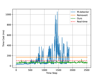
The proposed method maintains a consistently low time cost, well below the real-time threshold throughout the entire time span. This consistent performance highlights the efficiency of the proposed method in integrating front-end odometry and achieving real-time processing.

The red dashed line marks the real-time performance threshold. Both M-detector and Removert frequently exceed this threshold, indicating challenges in maintaining real-time performance. In contrast, the proposed method remains consistently below this line, indicating robust real-time performance.

In summary, the proposed method significantly outperforms M-detector and Removert in terms of time cost, maintaining real-time performance throughout the observed period. M-detector shows considerable variability and occasional spikes that disrupt real-time processing, while Removert, despite being more stable than M-detector, consistently exceeds the real-time threshold. These observations underscore the efficiency and stability of the proposed method in dynamic object labeling tasks, leveraging front-end odometry to achieve superior real-time performance.

inline]Discussion is short, you can merge with conclusion –Done

V Conclusion

In this paper, we propose a real-time dynamic object detection and tracking method for mobile robots equipped with LiDAR sensors. Our approach leverages front-end odometry to enable real-time detection of dynamic objects. By converting unordered LiDAR point cloud data into intensity images and applying a Gaussian Convolution Kernel, our method effectively segments feature points of foreground objects. These segmented points are then clustered into distinct objects and tracked within a sliding time window. This technique accumulates the transformation matrix between the current frame and the initial frame, allowing it to disregard historical drift and focus solely on the drift within the current window.

Our experiments demonstrate that this method achieves superior performance in dynamic object detection across four test sequences, significantly outperforming other state-of-the-art methods. The proposed system shows strong resilience to odometry drift, maintaining high detection accuracy and recall rates. Furthermore, it achieves real-time processing, ensuring reliable operation in dynamic environments over extended periods.

This solution presents a robust and efficient approach to real-time dynamic object detection and tracking, enabling mobile robots to navigate safely and effectively in environments with moving objects. By enhancing the system’s capability to manage both static and dynamic features, our method contributes to the development of more accurate and reliable SLAM systems for autonomous robotics.

However, the proposed method performs well in normal environments but is sensitive to object occlusion. When objects are blocked by other objects, the method loses track of them in the tracking process. Upon reappearance, the method treats them as new objects and tracks them from the initial frame. To address this issue, we can implement a data association method to compare the objects in the current frame with those in the previous 2 or 3 frames. If matches are found, we can maintain continuous tracking of the object from the initial frame. Alternatively, a Kalman filter [48] can be used to predict the object’s position when it is occluded. This approach will improve tracking accuracy and reduce tracking loss.

In addition to data association and Kalman filtering, exploring advanced feature matching techniques, such as deep learning-based object re-identification, could further enhance the robustness of the method against occlusion. By combining these strategies, the proposed method can achieve more reliable and precise tracking in dynamic environments, ultimately contributing to the development of more effective SLAM systems for various robotic applications.

Furthermore, integrating the proposed method into a SLAM (Simultaneous Localization and Mapping) system can enhance localization accuracy. By filtering out dynamic objects in the back-end of the SLAM system, we can eliminate ghost map points and refine the generated map. This integration will leverage the SLAM system’s ability to manage static and dynamic features, leading to more robust and accurate environmental mapping and object tracking.

Overall, this section addresses the limitations of our study and proposes future research directions. We suggest advancements in dynamic object tracking with a unstable ego-motion estimation, discuss the broader implications of our findings, and highlight potential applications of our method. This comprehensive overview underscores our contributions to the field of robotics, particularly in autonomous navigation.

Appendix A Appendix Section

A-A Detailed Analysis of Experimental Results

(a) Precision results in Sequence 1: This subfigure shows the precision results for the first sequence. The precision of each method is plotted, demonstrating the variability and performance across the sequence. Our method with front-end odometry achieves the highest and most stable precision throughout the sequence, significantly outperforming the other methods. M-detector with FAST-LIO also shows good performance but with more variability. Removert and M-detector with front-end odometry show lower precision.

(b) Precision results in Sequence 2: This subfigure displays the precision results for the second sequence. Similar to Sequence 1, our method with front-end odometry maintains the highest precision with minimal variability. M-detector with FAST-LIO again shows high precision but with notable fluctuations. Removert and M-detector with front-end odometry continue to perform poorly, indicating a consistent trend across different sequences.

(c) Precision results in Sequence 3: This subfigure presents the precision results for the third sequence. It highlights how each method performed in terms of precision throughout the sequence. Our method consistently achieves the highest precision, reinforcing its robustness and reliability. The performance of M-detector with FAST-LIO remains high but less stable compared to our method. Removert with A-LOAM has slightly lower precision to M-detector with FAST-LIO, but has more stable performance. Removert with front-end odometry exhibit similar lower precision trends as observed in previous sequences.

(d) Precision results in Sequence 4: This subfigure illustrates the precision results for the fourth sequence. It offers insights into the precision performance of each method in this sequence. Our method with front-end odometry once again leads with the highest precision and lowest variability. M-detector with FAST-LIO shows competitive precision but with occasional dips. Removert with A-LOAM still has similar performance with M-detector with FAST-LIO, but has more stable performance. Removert and M-detector with front-end odometry show the least precision, consistent with the patterns seen in the earlier sequences.

Figure A.1: Precision results across four sequences. This figure presents the precision results for different dynamic object detection methods across four test sequences. The methods compared are: M-detector with front-end odometry, Removert with front-end odometry, M-detector with FAST-LIO, Removert with A-LOAM, and our method with front-end odometry.

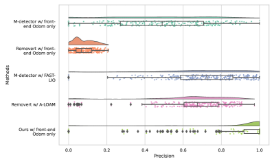
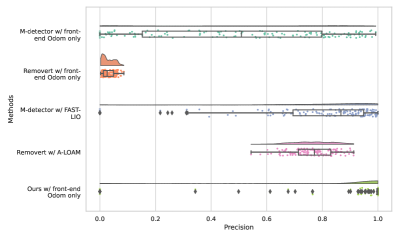
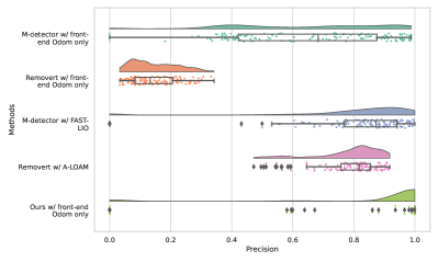
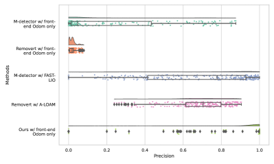
The experimental results shown in Figure A.1 provide a detailed comparison of the precision performance of different dynamic object detection methods across four sequences. The precision results across four sequences demonstrate the superiority and consistency of our method with front-end odometry. In Sequence 1, our method achieves the highest and most stable precision, significantly outperforming other methods such as M-detector with FAST-LIO and Removert with A-LOAM, which, while performing well, show greater variability. Removert and M-detector with front-end odometry exhibit lower precision and higher variability, indicating less reliability in dynamic object detection.

For Sequence 2, the precision results reinforce the findings from Sequence 1. Our method maintains the highest precision with minimal variability, demonstrating its robustness across different sequences. The performance of M-detector with FAST-LIO, although high in precision, shows notable fluctuations. The performance of Removert with A-LOAM has similar precision with M-detector with FAST-LIO, but lower variability. Meanwhile, Removert with front-end odometry and M-detector with front-end odometry continue to perform poorly, suggesting a consistent trend of lower precision and higher variability.

Sequence 3 precision results highlight the consistency and robustness of our method, which again achieves the highest precision throughout the sequence. M-detector with FAST-LIO remains a strong performer but with less stability compared to our method. The lower precision and higher variability observed in M-detector with front-end odometry, mirror the trends seen in previous sequences, underlining its limitations in dynamic object detection. Removert with A-LOAM in this sequence shows better performance compared to the earlier sequences, but still lags behind our method. Removert with front-end odometry continues to show the least precision, consistent with the earlier sequences, highlighting the challenges in maintaining accuracy with drift odometry.

The precision results in Sequence 4 further validate the effectiveness of our method, which leads with the highest precision and the least variability. M-detector with FAST-LIO shows competitive performance but with occasional dips in precision. Removert and M-detector with front-end odometry continue to show the least precision, consistent with the earlier sequences, highlighting the robustness and reliability of our approach.

(a) IoU results in Sequence 1: This subfigure presents the IoU results for the first sequence. Our method with front-end odometry achieves the highest IoU, indicating its effectiveness in accurately detecting dynamic objects. M-detector with FAST-LIO shows good IoU but with more variability. Removert with A-LOAM and M-detector with front-end odometry display lower IoU and higher variability, suggesting challenges in maintaining consistency.

(b) IoU results in Sequence 2: This subfigure shows the IoU results for the second sequence. Similar to the precision results, our method with front-end odometry achieves the highest IoU with minimal variability. M-detector with FAST-LIO also performs well but shows notable fluctuations. M-detector with front-end odometry continue to show lower IoU and higher variability. Removert has lower variability, but also has lower IoU.

(c) IoU results in Sequence 3: This subfigure presents the IoU results for the third sequence. Our method with front-end odometry consistently achieves the highest IoU, reinforcing its robustness. M-detector with FAST-LIO remains competitive but less stable. Removert with A-LOAM and M-detector with front-end odometry show similar lower IoU trends as observed previously.

(d) IoU results in Sequence 4: This subfigure illustrates the IoU results for the fourth sequence. Our method with front-end odometry once again leads with the highest IoU and lowest variability. M-detector with FAST-LIO shows competitive IoU but with occasional dips. Removert and M-detector with front-end odometry show the lowest IoU, consistent with the patterns seen in earlier sequences.

Figure A.2: IoU results across four sequences. This figure presents the IoU results for different dynamic object detection methods across four test sequences. The methods compared are: M-detector with front-end odometry, Removert with front-end odometry, M-detector with FAST-LIO, Removert with A-LOAM, and our method with front-end odometry.

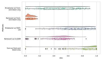
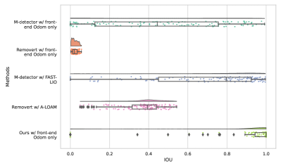
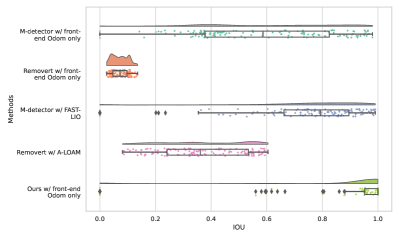
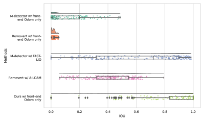
The IoU results in Figure A.2 across the sequences reinforce the trends observed in the precision analysis. In Sequence 1, our method with front-end odometry achieves the highest IoU, demonstrating its effectiveness in accurately detecting dynamic objects. M-detector with FAST-LIO shows good IoU but with greater variability. Removert with A-LOAM and M-detector with front-end odometry display lower IoU and higher variability, indicating challenges in maintaining consistency. The Removert with front-end odometry shows the least IoU among all methods.

In Sequence 2, our method maintains the highest IoU with minimal variability, similar to the precision results. M-detector with FAST-LIO performs well but with notable fluctuations. The lower IoU and higher variability with M-detector with front-end odometry and the least IoU in Removert with front-end odometry, further confirm their limitations in dynamic object detection when they equipped lower precision odometry.

The IoU results for Sequence 3 continue to show our method’s robustness, consistently achieving the highest IoU. M-detector with FAST-LIO remains competitive but less stable compared to our method. The trends of lower IoU and higher variability in Removert with A-LOAM and M-detector with front-end odometry, are consistent with previous observations.

For Sequence 4, our method once again leads with the highest IoU and the least variability. M-detector with FAST-LIO shows competitive IoU but with occasional dips. Removert and M-detector with front-end odometry continue to display the lowest IoU, aligning with the patterns seen in earlier sequences.

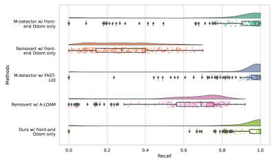
The recall results in Figure A.3 similarly highlight the robustness and effectiveness of our method. In Sequence 1, the recall performance of our method is notably similar to the M-detector with front-end odometry method. Among the methods, M-detector with FAST-LIO achieves the best recall results, demonstrating the highest recall values and the least variability. Despite this, our method remains highly competitive, exhibiting substantial recall performance that outperforms the other methods. Both our method and the M-detector with front-end odometry demonstrate superior recall results compared to the Removert methods, specifically Removert with front-end odometry and Removert with A-LOAM, which consistently show lower recall values and higher variability.

Sequence 2 recall results demonstrate that our method has the highest recall with minimal variability. M-detector with FAST-LIO shows high recall but notable fluctuations. M-detector with front-end odometry also exhibits competitive recall, although with more variability. The lower recall and higher variability in Removert with A-LOAM and Removert with front-end odometry, indicate consistent poor performance across different sequences.

In Sequence 3, our method consistently achieves the highest recall, reinforcing its robustness. M-detector remains high in recall but less stable. However, in this sequence, the M-detector with front-end odometry has better performance than M-detector with FAST-LIO. Removert with A-LOAM and M-detector with front-end odometry show similar lower recall trends as previously observed.

The recall results in Sequence 4 further illustrate the effectiveness of our method, leading with the highest recall and lowest variability. M-detector with FAST-LIO shows competitive recall but with occasional dips. However, in this sequence M-detector with front-end odometry’s recall performance is not as good as previous sequences. It has similir lower recall as Removert with front-end odometry . Removert with A-LOAM preformes better than before but still has lower recall compared to M-detector with FAST-LIO and our method.

(a) Recall results in Sequence 1: This subfigure shows the recall results for the first sequence. M-detector with FAST-LIO achieves the best recall with the least variability. Our method with front-end odometry remains competitive, outperforming Removert methods, which show lower recall and higher variability.

(b) Recall results in Sequence 2: This subfigure displays the recall results for the second sequence. Our method achieves the highest recall with minimal variability. M-detector with FAST-LIO shows high recall with fluctuations. Removert methods continue to perform poorly with lower recall.

(c) Recall results in Sequence 3: This subfigure presents the recall results for the third sequence. Our method consistently achieves the highest recall. M-detector with front-end odometry performs better than M-detector with FAST-LIO. Removert methods show similar lower recall trends.

(d) Recall results in Sequence 4: This subfigure illustrates the recall results for the fourth sequence. Our method leads with the highest recall and lowest variability. M-detector with FAST-LIO shows competitive recall but with occasional dips. M-detector with front-end odometry and Removert methods perform worse compared to previous sequences.

Figure A.3: Recall results across four sequences. This figure presents the recall results for different dynamic object detection methods across four test sequences. The methods compared are: M-detector with front-end odometry, Removert with front-end odometry, M-detector with FAST-LIO, Removert with A-LOAM, and our method with front-end odometry.

(a) F1 Score results in Sequence 1: This subfigure demonstrates our method with front-end odometry achieving the highest and most consistent F1 Score, significantly outperforming the other methods. M-detector with FAST-LIO shows competitive scores but with notable variability. Removert with A-LOAM and M-detector with front-end odometry exhibit lower F1 Scores and increased variability. Removert with A-LOAM shows slight better performance compared with other sequences.

(b) F1 Score results in Sequence 2: Our method continues to maintain the highest F1 Score with minimal variability, echoing the precision and recall outcomes. M-detector with FAST-LIO, although high, exhibits significant fluctuations. Both Removert and M-detector with front-end odometry confirm their weaker performance under noisy conditions by showing lower scores or higher variability.

(c) F1 Score results in Sequence 3: This subfigure highlights the robustness of our method, consistently achieving the highest F1 Score. M-detector with FAST-LIO remains competitive but but less stable. M-detector with front-end odometry outperforms Removert with A-LOAM in this sequence, though both continue to demonstrate high variability and lower scores.

(d) F1 Score results in Sequence 4: Our method leads with the highest F1 Score and lowest variability, confirming its consistent performance across sequences. M-detector with FAST-LIO remains competitive but with decreased stability. Removert with front-end odometry consistently shows the lowest F1 Scores, consistent with earlier patterns, while M-detector with front-end odometry displays similar scores but with increased variability.

Figure A.4: F1 Score results across four sequences. This figure presents the F1 Score results for different dynamic object detection methods across four test sequences. The methods compared are: M-detector with front-end odometry, Removert with front-end odometry, M-detector with FAST-LIO, Removert with A-LOAM, and our method with front-end odometry.

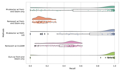
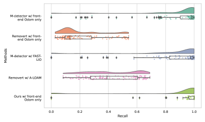
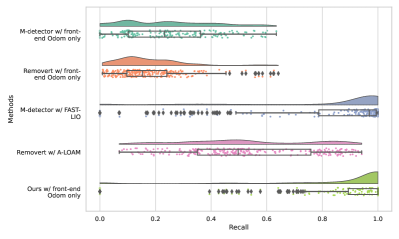
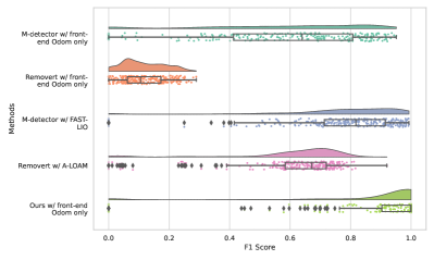
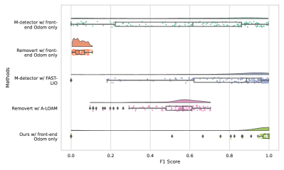
The F1 Score results in Figure A.4 across the sequences provide a comprehensive view of our method’s performance. In Sequence 1, our method with front-end odometry achieves the highest and most stable F1 Score, significantly outperforming other methods. M-detector with FAST-LIO shows good F1 Score but with more variability, while Removert with A-LOAM and M-detector with front-end odometry show lower F1 Score and M-detector with front-end odometry shows higher variability. Removert with A-LOAM shows better F1 score compared with the performance in other sequences. The Removert with front-end odometry has the lowest F1 Score among all methods.

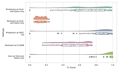
For Sequence 2, our method maintains the highest F1 Score with minimal variability, similar to the precision and recall results. M-detector with FAST-LIO shows high F1 Score but notable fluctuations. The lower F1 Score in Removert with front-end odometry and the higher variability of M-detector with front-end odometry, further confirm their consistent poor performance during noisy odometry.

Sequence 3 F1 Score results reinforce our method’s robustness, consistently achieving the highest F1 Score. M-detector with FAST-LIO remains competitive but less stable. The M-detector with front-end odometry has better F1 score than Removert with A-LOAM, but they all have higher variability. The lowest F1 Score in Removert with front-end odometry is consistent with previous observations.

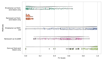
In Sequence 4, our method once again leads with the highest F1 Score and lowest variability. M-detector with FAST-LIO shows competitive F1 Score but with even worse stability compared the performance in the previous sequences. Removert with front-end odometry continue to display the lowest F1 Score, aligning with the patterns seen in earlier sequences. M-detector with front-end odometry has similar F1 Score as Removert with front-end odometry, but with higher variability.

Overall, the detailed analysis of experimental results across precision, IoU, recall, and F1 score consistently highlights the superiority and robustness of our method with front-end odometry. The consistent high performance and low variability of our method across different sequences underscore its reliability and effectiveness in dynamic object detection.

Additionally, we performed statistical analysis using the Wilcoxon Signed-Rank Test [49] to evaluate the significance of the differences between the methods. We selected the Wilcoxon Signed-Rank Test because some of the data for precision, IoU, recall, and F1 score do not follow the normal distribution, and some data present outliers or extreme values, such as 0 or 1. Therefore, the Wilcoxon Signed-Rank Test is well-suited for this analysis. The results demonstrate that our method with front-end odometry significantly outperforms the other methods in terms of precision, IoU, recall, and F1 score, with all p-values $<0.05$. This statistical analysis further confirms the superior performance of our method in dynamic object detection.

Appendix B Biography Section

Wenqiang Du received the B.E. degree in the mechanical engineering from the Anhui University, Hefei, China in 2016, and the M.E. degree in the Pattern Recongnition and Intelligent System from the University of Chinese Academy of Sciences, Beijing, China in 2019. He is currently working towards the Ph.D. degree in the MISTLab, the Department of Computer Engineering and Software Engineering, Polytechnique Montreal. His research interests include SLAM, robotics, perception, and dynamic objects detection.

Giovanni Beltrame (Senior Member, IEEE) obtained his Ph. D. in Computer Engineering from Politecnico di Milano in 2006. He worked as microelectronics engineer at the European Space Agency on a number of projects, spanning from radiation tolerant systems to computer-aided design. Since 2010 he is Professor at Polytechnique Montreal with the Computer and Software Engineering Department, where he directs the MIST Lab and the ASTROLITH research group. He has authored or coauthored more than 100 papers in international journals and conferences. His research interests include modeling and design of embedded systems, artificial intelligence, and robotics.

References

- [1] C. Campos, R. Elvira, J. J. G. Rodríguez, J. M. Montiel, and J. D. Tardós, “ORB-SLAM3: An Accurate Open-Source Library for Visual, Visual-Inertial, and Multimap SLAM,” IEEE Transactions on Robotics, 2021.
- [2] J. Zhang and S. Singh, “LOAM: Lidar odometry and mapping in real-time.” in Robotics: Science and systems, vol. 2, no. 9. Berkeley, CA, 2014, pp. 1–9.
- [3] T. Qin, P. Li, and S. Shen, “VINS-Mono: A robust and versatile monocular visual-inertial state estimator,” IEEE Transactions on Robotics, vol. 34, no. 4, pp. 1004–1020, 2018.
- [4] W. Xu, Y. Cai, D. He, J. Lin, and F. Zhang, “FAST-LIO2: Fast direct lidar-inertial odometry,” IEEE Transactions on Robotics, 2022.
- [5] T. Shan, B. Englot, C. Ratti, and D. Rus, “LVI-SAM: Tightly-coupled Lidar-Visual-Inertial Odometry via Smoothing and Mapping,” in 2021 IEEE international conference on robotics and automation (ICRA). IEEE, 2021, pp. 5692–5698.
- [6] T. Shan, B. Englot, D. Meyers, W. Wang, C. Ratti, and R. Daniela, “LIO-SAM: Tightly-coupled Lidar Inertial Odometry via Smoothing and Mapping,” in IEEE/RSJ International Conference on Intelligent Robots and Systems (IROS). IEEE, 2020, pp. 5135–5142.
- [7] P. Furgale, U. Schwesinger, M. Rufli, W. Derendarz, H. Grimmett, P. Mühlfellner, S. Wonneberger, J. Timpner, S. Rottmann, B. Li et al., “Toward automated driving in cities using close-to-market sensors: An overview of the v-charge project,” in 2013 IEEE Intelligent Vehicles Symposium (IV). IEEE, 2013, pp. 809–816.
- [8] H. Peng, Z. Zhao, and L. Wang, “A Review of Dynamic Object Filtering in SLAM Based on 3D LiDAR,” Sensors, vol. 24, no. 2, p. 645, 2024.
- [9] J. Redmon, S. Divvala, R. Girshick, and A. Farhadi, “You Only Look Once: Unified, Real-Time Object Detection,” in Proceedings of the IEEE conference on computer vision and pattern recognition, 2016, pp. 779–788.
- [10] J. Redmon and A. Farhadi, “YOLO9000: better, faster, stronger,” in Proceedings of the IEEE conference on computer vision and pattern recognition, 2017, pp. 7263–7271.
- [11] A. Farhadi and J. Redmon, “YOLOv3: An incremental improvement,” in Computer vision and pattern recognition, vol. 1804. Springer Berlin/Heidelberg, Germany, 2018, pp. 1–6.
- [12] A. Bochkovskiy, C.-Y. Wang, and H.-Y. M. Liao, “YOLOv4: Optimal speed and accuracy of object detection,” arXiv preprint arXiv:2004.10934, 2020.
- [13] Z. Ge, S. Liu, F. Wang, Z. Li, and J. Sun, “YOLOX: Exceeding YOLO Series in 2021,” arXiv preprint arXiv:2107.08430, 2021.
- [14] H. Lim, S. Hwang, and H. Myung, “Erasor: Egocentric ratio of pseudo occupancy-based dynamic object removal for static 3d point cloud map building,” IEEE Robotics and Automation Letters, vol. 6, no. 2, pp. 2272–2279, 2021.
- [15] E. Arani, S. Gowda, R. Mukherjee, O. Magdy, S. Kathiresan, and B. Zonooz, “A comprehensive study of real-time object detection networks across multiple domains: A survey,” arXiv preprint arXiv:2208.10895, 2022.
- [16] L. Schmid, O. Andersson, A. Sulser, P. Pfreundschuh, and R. Siegwart, “Dynablox: Real-time detection of diverse dynamic objects in complex environments,” IEEE Robotics and Automation Letters, 2023.
- [17] W. Du and G. Beltrame, “Real-time simultaneous localization and mapping with lidar intensity,” in 2023 IEEE International Conference on Robotics and Automation (ICRA). IEEE, 2023, pp. 4164–4170.
- [18] H. Wu, Y. Li, W. Xu, F. Kong, and F. Zhang, “Moving event detection from lidar point streams,” Nature Communications, vol. 15, no. 1, p. 345, 2024.
- [19] G. Kim and A. Kim, “Remove, then revert: Static point cloud map construction using multiresolution range images,” in 2020 IEEE/RSJ International Conference on Intelligent Robots and Systems (IROS). IEEE, 2020, pp. 10 758–10 765.
- [20] A. Azim and O. Aycard, “Detection, classification and tracking of moving objects in a 3d environment,” in 2012 IEEE Intelligent Vehicles Symposium. IEEE, 2012, pp. 802–807.
- [21] J. Schauer and A. Nüchter, “The peopleremover—removing dynamic objects from 3-d point cloud data by traversing a voxel occupancy grid,” IEEE robotics and automation letters, vol. 3, no. 3, pp. 1679–1686, 2018.
- [22] S. Thrun, “Learning occupancy grid maps with forward sensor models,” Autonomous robots, vol. 15, pp. 111–127, 2003.
- [23] A. Hornung, K. M. Wurm, M. Bennewitz, C. Stachniss, and W. Burgard, “Octomap: An efficient probabilistic 3d mapping framework based on octrees,” Autonomous robots, vol. 34, pp. 189–206, 2013.
- [24] L. Schmid, M. Abate, Y. Chang, and L. Carlone, “Khronos: A unified approach for spatio-temporal metric-semantic slam in dynamic environments,” arXiv preprint arXiv:2402.13817, 2024.
- [25] H. Lim, L. Nunes, B. Mersch, X. Chen, J. Behley, H. Myung, and C. Stachniss, “Erasor2: Instance-aware robust 3d mapping of the static world in dynamic scenes,” in Robotics: Science and Systems (RSS 2023). IEEE, 2023.
- [26] F. Pomerleau, P. Krüsi, F. Colas, P. Furgale, and R. Siegwart, “Long-term 3d map maintenance in dynamic environments,” in 2014 IEEE International Conference on Robotics and Automation (ICRA). IEEE, 2014, pp. 3712–3719.
- [27] N. Banerjee, D. Lisin, J. Briggs, M. Llofriu, and M. E. Munich, “Lifelong mapping using adaptive local maps,” in 2019 European Conference on Mobile Robots (ECMR). IEEE, 2019, pp. 1–8.
- [28] R. Ambruş, N. Bore, J. Folkesson, and P. Jensfelt, “Meta-rooms: Building and maintaining long term spatial models in a dynamic world,” in 2014 IEEE/RSJ international conference on intelligent robots and systems. IEEE, 2014, pp. 1854–1861.
- [29] C. Jiang, D. P. Paudel, Y. Fougerolle, D. Fofi, and C. Demonceaux, “Static-map and dynamic object reconstruction in outdoor scenes using 3-d motion segmentation,” IEEE Robotics and Automation Letters, vol. 1, no. 1, pp. 324–331, 2016.
- [30] E. Palazzolo, J. Behley, P. Lottes, P. Giguere, and C. Stachniss, “Refusion: 3d reconstruction in dynamic environments for rgb-d cameras exploiting residuals,” in 2019 IEEE/RSJ International Conference on Intelligent Robots and Systems (IROS). IEEE, 2019, pp. 7855–7862.
- [31] B. Curless and M. Levoy, “A volumetric method for building complex models from range images,” in Proceedings of the 23rd annual conference on Computer graphics and interactive techniques, 1996, pp. 303–312.
- [32] L. Nunes, X. Chen, R. Marcuzzi, A. Osep, L. Leal-Taixé, C. Stachniss, and J. Behley, “Unsupervised class-agnostic instance segmentation of 3d lidar data for autonomous vehicles,” IEEE Robotics and Automation Letters, vol. 7, no. 4, pp. 8713–8720, 2022.
- [33] H. Thomas, M. G. de Saint Aurin, J. Zhang, and T. D. Barfoot, “Learning spatiotemporal occupancy grid maps for lifelong navigation in dynamic scenes,” in 2022 International Conference on Robotics and Automation (ICRA). IEEE, 2022, pp. 484–490.
- [34] H. Thomas, C. R. Qi, J.-E. Deschaud, B. Marcotegui, F. Goulette, and L. J. Guibas, “Kpconv: Flexible and deformable convolution for point clouds,” in Proceedings of the IEEE/CVF international conference on computer vision, 2019, pp. 6411–6420.
- [35] O. Ronneberger, P. Fischer, and T. Brox, “U-net: Convolutional networks for biomedical image segmentation,” in Medical image computing and computer-assisted intervention–MICCAI 2015: 18th international conference, Munich, Germany, October 5-9, 2015, proceedings, part III 18. Springer, 2015, pp. 234–241.
- [36] X. Chen, S. Li, B. Mersch, L. Wiesmann, J. Gall, J. Behley, and C. Stachniss, “Moving object segmentation in 3d lidar data: A learning-based approach exploiting sequential data,” IEEE Robotics and Automation Letters, vol. 6, no. 4, pp. 6529–6536, 2021.
- [37] A. Milioto, I. Vizzo, J. Behley, and C. Stachniss, “Rangenet++: Fast and accurate lidar semantic segmentation,” in 2019 IEEE/RSJ international conference on intelligent robots and systems (IROS). IEEE, 2019, pp. 4213–4220.
- [38] S. Li, X. Chen, Y. Liu, D. Dai, C. Stachniss, and J. Gall, “Multi-scale interaction for real-time lidar data segmentation on an embedded platform,” IEEE Robotics and Automation Letters, vol. 7, no. 2, pp. 738–745, 2021.
- [39] T. Cortinhal, G. Tzelepis, and E. Erdal Aksoy, “Salsanext: Fast, uncertainty-aware semantic segmentation of lidar point clouds,” in Advances in Visual Computing: 15th International Symposium, ISVC 2020, San Diego, CA, USA, October 5–7, 2020, Proceedings, Part II 15. Springer, 2020, pp. 207–222.
- [40] J. Sun, Y. Dai, X. Zhang, J. Xu, R. Ai, W. Gu, and X. Chen, “Efficient spatial-temporal information fusion for lidar-based 3d moving object segmentation,” in 2022 IEEE/RSJ International Conference on Intelligent Robots and Systems (IROS). IEEE, 2022, pp. 11 456–11 463.
- [41] B. Mersch, X. Chen, I. Vizzo, L. Nunes, J. Behley, and C. Stachniss, “Receding moving object segmentation in 3d lidar data using sparse 4d convolutions,” IEEE Robotics and Automation Letters, vol. 7, no. 3, pp. 7503–7510, 2022.
- [42] C. Choy, J. Gwak, and S. Savarese, “4d spatio-temporal convnets: Minkowski convolutional neural networks,” in Proceedings of the IEEE/CVF conference on computer vision and pattern recognition, 2019, pp. 3075–3084.
- [43] E. Rublee, V. Rabaud, K. Konolige, and G. Bradski, “Orb: An efficient alternative to sift or surf,” in 2011 International conference on computer vision. Ieee, 2011, pp. 2564–2571.
- [44] Y. Bar-Shalom and X.-R. Li, Multitarget-multisensor tracking: principles and techniques. YBS publishing Storrs, CT, 1995, vol. 19.
- [45] H. W. Kuhn, “The hungarian method for the assignment problem,” Naval research logistics quarterly, vol. 2, no. 1-2, pp. 83–97, 1955.
- [46] C. Goutte and E. Gaussier, “A probabilistic interpretation of precision, recall and f-score, with implication for evaluation,” in European conference on information retrieval. Springer, 2005, pp. 345–359.
- [47] G. Kim, “SC-A-LOAM,” https://github.com/gisbi-kim/SC-A-LOAM, 2021, accessed: 2021-07-16.
- [48] R. E. Kalman, “A new approach to linear filtering and prediction problems,” 1960.
- [49] F. Wilcoxon, “Individual comparisons by ranking methods,” in Breakthroughs in statistics: Methodology and distribution. Springer, 1992, pp. 196–202.